311 Feature Selection. 312 Goals –What is Feature Selection for classification? –Why feature...
67
1 Feature Selection Feature Selection
-
Upload
rosamond-anastasia-haynes -
Category
Documents
-
view
236 -
download
10
Transcript of 311 Feature Selection. 312 Goals –What is Feature Selection for classification? –Why feature...

1
Feature SelectionFeature Selection

2
GoalsGoals
– What is Feature Selection for classification?– Why feature selection is important?– What is the filter and what is the wrapper
approach to feature selection?– Examples

3
What is Feature Selection for What is Feature Selection for classification?classification?
– Given: a set of predictors (“features”) V and a target variable T
– Find: minimum set F that achieves maximum classification performance of T (for a given set of classifiers and classification performance metrics)
4
Why feature selection is important?Why feature selection is important?
– May Improve performance of classification algorithm
– Classification algorithm may not scale up to the size of the full feature set either in sample or time
– Allows us to better understand the domain– Cheaper to collect a reduced set of predictors– Safer to collect a reduced set of predictors

5
Filters vs Wrappers: WrappersFilters vs Wrappers: Wrappers
Say we have predictors A, B, C and classifier M. We want to predict T given the smallest possible subset of {A,B,C}, while achieving maximal performance (accuracy)
FEATURE SET CLASSIFIER PERFORMANCE
{A,B,C} M 98%
{A,B} M 98%
{A,C} M 77%
{B,C} M 56%
{A} M 89%
{B} M 90%
{C} M 91%
{.} M 85%

6
Filters vs Wrappers: WrappersFilters vs Wrappers: WrappersThe set of all subsets is the power set and its size is 2|V| . Hence for large V we cannot do this procedure exhaustively; instead we rely on heuristic search of the space of all possible feature subsets.
{} 85
{A} 89
{B} 90
{A,B} 98
{A,B,C}98
{C} 91
{A,C} 77
{B,C} 56
start
{A,B}98
{B,C}56
{A,C}77end

7
Filters vs Wrappers: WrappersFilters vs Wrappers: Wrappers
A common example of heuristic search is hill climbing: keep adding features one at a time until no further improvement can be achieved.
{} 85
{A} 89
{B} 90
{A,B} 98
{A,B,C}98
{C} 91
{A,C} 77
{B,C} 56
start
{A,B}98
{B,C}56
{A,C}77end

8
Filters vs Wrappers: WrappersFilters vs Wrappers: Wrappers
A common example of heuristic search is hill climbing: keep adding features one at a time until no further improvement can be achieved (“forward greedy wrapping”)
Alternatively we can start with the full set of predictors and keep removing features one at a time until no further improvement can be achieved (“backward greedy wrapping”)
A third alternative is to interleave the two phases (adding and removing) either in forward or backward wrapping (“forward-backward wrapping”).
Of course other forms of search can be used; most notably:
-Exhaustive search
-Genetic Algorithms
-Branch-and-Bound (e.g., cost=# of features, goal is to reach performance th or better)

9
Filters vs Wrappers: FiltersFilters vs Wrappers: Filters
In the filter approach we do not rely on running a particular classifier and searching in the space of feature subsets; instead we select features on the basis of statistical properties. A classic example is univariate associations:
FEATURE ASSOCIATION WITH TARGET
{A} 89%
{B} 90%
{C} 91%
Threshold gives suboptimal solution
Threshold gives suboptimal solution
Threshold gives optimal solution

10
Example Feature Selection Methods in Example Feature Selection Methods in Biomedicine: Univariate Association FilteringBiomedicine: Univariate Association Filtering
– Order all predictors according to strength of association with target
– Choose the first k predictors and feed them to the classifier
– Various measures of association may be used: X2, G2, Pearson r, Fisher Criterion Scoring, etc.
– How to choose k?
– What if we have too many variables?

11
Example Feature Selection Methods in Example Feature Selection Methods in Biomedicine: Recursive Feature EliminationBiomedicine: Recursive Feature Elimination
– Filter algorithm where feature selection is done as follows:
1. build linear Support Vector Machine classifiers using V features
2. compute weights of all features and choose the best V/2
3. repeat until 1 feature is left
4. choose the feature subset that gives the best performance (using cross-validation)
12
Example Feature Selection Methods in Example Feature Selection Methods in Bioinformatics: GA/KNNBioinformatics: GA/KNN
Wrapper approach whereby:
• heuristic search=Genetic Algorithm, and
• classifier=KNN

13
How do we approach the feature How do we approach the feature selection problem in our research?selection problem in our research?
– Find the Markov Blanket
– Why?

14
A fundamental property of the Markov BlanketA fundamental property of the Markov Blanket
– MB(T) is the minimal set of predictor variables needed for classification (diagnosis, prognosis, etc.) of the target variable T (given a powerful enough classifier and calibrated classification)
C D
T H
I
VV
V
V
V
V
V
V
VV
VVV
V
V
V
V
V
V
VV
VV
V
V
V
V
V
V
VV
VVV
V
V
V
V
V
V
VV

15
HITON: An algorithm for feature selection HITON: An algorithm for feature selection that combines MB induction with wrappingthat combines MB induction with wrapping
C.F. Aliferis M.D., Ph.D., I. Tsamardinos Ph.D., A. Statnikov M.S.
Department of Biomedical Informatics, Vanderbilt University
AMIA Fall Conference, November 2003

16
HITON: An algorithm for feature selection that combines HITON: An algorithm for feature selection that combines MB induction with wrappingMB induction with wrapping
ALGORITHM SOUND SCALABLE SAMPLE EXPONENTIAL
TO |MB|
COMMENTS
Cheng and Greiner YES NO NO Post-processing on learning BN
Cooper et al. NO NO NO Uses full BN learning
Margaritis and Thrun
YES YES YES Intended to facilitate BN
learning
Koller and Sahami NO NO NO Most widely-cited MB induction algorithm
Tsamardinos and Aiferis
YES YES YES Some use BN learning as sub-
routine
HITON YES YES NO

17
HITON: An algorithm for feature selection HITON: An algorithm for feature selection that combines MB induction with wrappingthat combines MB induction with wrapping
Step #1: Find the parents and children of T; call this set PC(T)
Step #2: Find the PC(.) set of each member of PC(T); take the union of all these sets to be PCunion
Step #3: Run a special test to filter out from PCunion the non-members of MB(T) that can be identified as such (not all can); call the resultant set TMB (tentative MB)
Step #4: Apply heuristic search with a desired classifier/loss function and cross-validation to identify variables that can be dropped from TMB without loss of accuracy
18
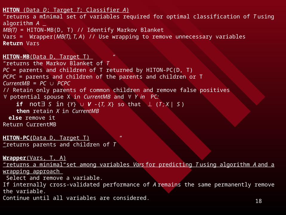
HITON (Data D; Target T; Classifier A)“returns a minimal set of variables required for optimal classification of T using algorithm A” MB(T) = HITON-MB(D, T) // Identify Markov BlanketVars = Wrapper(MB(T), T, A) // Use wrapping to remove unnecessary variablesReturn Vars HITON-MB(Data D, Target T) “returns the Markov Blanket of T”PC = parents and children of T returned by HITON-PC(D, T)PCPC = parents and children of the parents and children or TCurrentMB = PC PCPC// Retain only parents of common children and remove false positives potential spouse X in CurrentMB and Y inPC: if not S in {Y} V -{T, X} so that (T ; X | S ) then retain X in CurrentMB else remove it Return CurrentMB HITON-PC(Data D, Target T)“returns parents and children of T”
Wrapper(Vars, T, A)“returns a minimal set among variables Vars for predicting T using algorithm A and a wrapping approach” Select and remove a variable.If internally cross-validated performance of A remains the same permanently remove the variable.Continue until all variables are considered.

19
HITON-PC(Data D, Target T)“returns parents and children of T”CurrentPC = {}RepeatFind variable Vi not in CurrentPC that maximizes association(Vi, T) and admit Vi into CurrentPC
If there is a variable X and a subset S of CurrentPC s.t. (X : T | S) remove Vi from CurrentPC;
mark Vi and do not consider it again
Until no more variables are left to consider Return CurrentPC

20
Dataset Thrombin Arrythmia Ohsumed Lung Cancer Prostate Cancer Problem Type Drug
Discovery Clinical Diagnosis
Text Categorization
Gene Expression Diagnosis
Mass-Spec Diagnosis
Variable # 139,351 279 14,373 12,600 779 Variable Types binary nominal/ordinal
/continuous binary and continuous
continuous continuous
Target binary nominal binary binary binary Sample 2,543 417 2000 160 326 Vars-to-Sample 54.8 0.67 7.2 60 2.4 Evaluation metric ROC AUC Accuracy ROC AUC ROC AUC ROC AUC Design 1-fold c.v. 10-fold c.v. 1-fold c.v. 5-fold c.v. 10-fold c.v.
Figure 2: Dataset Characteristics

21

22

23
Filters vs Wrappers: Which Is Best?Filters vs Wrappers: Which Is Best?
None over all possible classification tasks! We can only prove that a specific filter (or
wrapper) algorithm for a specific classifier (or class of classifiers), and a specific class of distributions yields optimal or sub-optimal solutions. Unless we provide such proofs we are operating on faith and hope…

24
A final note: What is the biological A final note: What is the biological significance of selected features?significance of selected features?
In MB-based feature selection and CPN-faithful distributions: causal neighborhood of target (i.e., direct causes, direct effects, direct causes of the direct effects of target).
In other methods: ???

25
Case StudiesCase Studies

26
Case Study: Categorizing Text Into Case Study: Categorizing Text Into Content CategoriesContent Categories
Automatic Identification of Purpose and Quality of Articles In Journals Of Internal Medicine
Yin Aphinyanaphongs M.S. ,
Constantin Aliferis M.D., Ph.D.
(presented in AMIA 2003)

27
Case Study: Categorizing Text Into Case Study: Categorizing Text Into Content CategoriesContent Categories
The problem: classify Pubmed articles as [high quality & treatment specific]
or not Same function as the current Clinical
Quality Filters of Pubmed (in the treatment category)

28

29
Case Study: Categorizing Text Into Case Study: Categorizing Text Into Content CategoriesContent Categories
Overview:– Select Gold Standard– Corpus Construction– Document representation– Cross-validation Design– Train classifiers– Evaluate the classifiers

30
Case Study: Categorizing Text Into Case Study: Categorizing Text Into Content CategoriesContent Categories
Select Gold Standard:– ACP journal club. Expert reviewers strictly evaluate and
categorize in each medical area articles from the top journals in internal medicine.
– Their mission is “to select from the biomedical literature those articles reporting original studies and systematic reviews that warrant immediate attention by physicians.”
The treatment criteria -ACP journal club– “Random allocation of participants to comparison groups.”
– “80% follow up of those entering study.”
– “Outcome of known or probable clinical importance.”
If an article is cited by the ACP , it is a high quality article.

31
Case Study: Categorizing Text Into Case Study: Categorizing Text Into Content CategoriesContent Categories
Corpus construction:
12/2000
8/1998 9/1999
Get all articles from the 49 journals in the study period.
Review ACP Journal from 8/1998 to 12/2000 for articles that are cited by the ACP.
15,803 total articles, 396 positives (high quality treatment related)

32
Case Study: Categorizing Text Into Case Study: Categorizing Text Into Content CategoriesContent Categories
Document representation:– “Bag of words”– Title, abstract, Mesh terms, publication type– Term extraction and processing: e.g. “The clinical
significance of cerebrospinal.”
1. Term extraction» “The”, “clinical”, “significance”, “of”, “cerebrospinal”
2. Stop word removal» “Clinical”, “Significance”, “Cerebrospinal”
3. Porter Stemming (i.e. getting the roots of words)» “Clinic*”, “Signific*”, “Cerebrospin*”
4. Term weighting» log frequency with redundancy.

33
Case Study: Categorizing Text Into Case Study: Categorizing Text Into Content CategoriesContent Categories
Cross-validation design
15803 articles
20% reserve
80%
train
validation
test
10 fold crossValidation to measureerror

34
Case Study: Categorizing Text Into Case Study: Categorizing Text Into Content CategoriesContent Categories
Classifier families– Naïve Bayes (no parameter optimization)– Decision Trees with Boosting (# of iterations =
# of simple rules)– Linear & Polynomial Support Vector Machines
(cost from {0.1, 0.2, 0.4, 0.7, 0.9, 1, 5, 10, 20, 100, 1000}, degree from {1,2,3,5,8})
35
Case Study: Categorizing Text Into Case Study: Categorizing Text Into Content CategoriesContent Categories
Evaluation metrics (averaged over 10 cross-validation folds):– Sensitivity for fixed specificity – Specificity for fixed sensitivity– Area under ROC curve– Area under 11-point precision-recall curve– “Ranked retrieval”
36
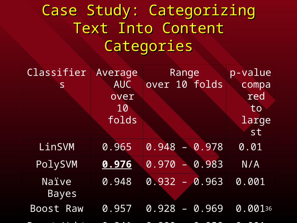
Case Study: Categorizing Text Into Case Study: Categorizing Text Into Content CategoriesContent Categories
Classifiers Average AUC
over 10 folds
Rangeover 10 folds
p-value compar
ed to largest
LinSVM 0.965 0.948 – 0.978 0.01
PolySVM 0.976 0.970 – 0.983 N/A
Naïve Bayes 0.948 0.932 – 0.963 0.001
Boost Raw 0.957 0.928 – 0.969 0.001
Boost Wght 0.941 0.900 – 0.958 0.001

37
Case Study: Categorizing Text Into Case Study: Categorizing Text Into Content CategoriesContent Categories
Sensitivity Specificity Precision
Number Needed to Read(Average)
CQF 0.367 0.959 0.149 6.7
PolySVM
0.8181
(0.641-0.93)
0.959
(0.948-0.97)
0.2816
(0.191-0.388)
3.55
Sensitivity Specificity Precision
Number Needed to Read(Average)
CQF 0.96 0.75 0.071 14
PolySVM
0.9673(0.830-0.99)
0.8995(0.884-0.914)
0.1744(0.120-0.240)
6

38
Case Study: Categorizing Text Into Case Study: Categorizing Text Into Content CategoriesContent Categories
Clinical Query Filter Performance
36
18
9
27
Clinical Query Filter

39
Case Study: Categorizing Text Into Case Study: Categorizing Text Into Content CategoriesContent Categories
Clinical Query Filter

40
Case Study: Categorizing Text Into Case Study: Categorizing Text Into Content CategoriesContent Categories
Alternative/additional approaches?– Negation detection– Citation analysis– Sequence of words– Variable selection to produce user-
understandable models– Analysis of ACPJ potential bias– Others???

41
Case Study: Diagnostic Model From Case Study: Diagnostic Model From Array Gene Expression DataArray Gene Expression Data
Computational Models of Lung Cancer: Connecting Classification, Gene Selection, and Molecular
Sub-typing
C.Aliferis M.D., Ph.D., Pierre Massion M.D.I. Tsamardinos Ph.D., D. Hardin Ph.D.

42
Case Study: Diagnostic Model From Case Study: Diagnostic Model From Array Gene Expression DataArray Gene Expression Data
Specific Aim 1: “Construct computational models that distinguish between important cellular states related to lung cancer, e.g., (i) Cancerous vs Normal Cells; (ii) Metastatic vs Non-Metastatic cells; (iii) Adenocarcinomas vs Squamous carcinomas”.
Specific Aim 2: “Reduce the number of gene markers by application of biomarker (gene) selection algorithms such that small sets of genes can distinguish among the different states (and ideally reveal important genes in the pathophysiology of lung cancer).”
43
Case Study: Diagnostic Model From Case Study: Diagnostic Model From Array Gene Expression DataArray Gene Expression Data
Bhattacharjee et al. PNAS, 2001 12,600 gene expression measurements
obtained using Affymetrix oligonucleotide arrays
203 patients and normal subjects, 5 disease types, ( plus staging and survival information)

44
Case Study: Diagnostic Model From Case Study: Diagnostic Model From Array Gene Expression DataArray Gene Expression Data
Linear and polynomial-kernel Support Vector Machines (LSVM, and PSVM respectively)
C optimized via C.V. from {10-8, 10-7, 10-6, 10-5, 10-4, 10-3, 10-2, 0.1, 1, 10, 100, 1000} and degree from the set: {1, 2, 3, 4}.
K-Nearest Neighbors (KNN) (k optimized via C.V.) Feed-forward Neural Networks (NNs). 1 hidden layer, number of units
chosen (heuristically) from the set {2, 3, 5, 8, 10, 30, 50}, variable-learning-rate back propagation, custom-coded early stopping with (limiting) performance goal=10-8 (i.e., an arbitrary value very close to zero), and number of epochs in the range [100,…,10000], and a fixed momentum of 0.001
Stratified nested n-fold cross-validation (n=5 or 7 depending on task)

45
Case Study: Diagnostic Model From Case Study: Diagnostic Model From Array Gene Expression DataArray Gene Expression Data
Area under the Receiver Operator Characteristic (ROC) curve (AUC) computed with the trapezoidal rule (DeLong et al. 1998).
Statistical comparisons among AUCs were performed using a paired Wilcoxon rank sum test (Pagano et al. 2000).
Scale gene values linearly to [0,1]
Feature selection:– RFE (parameters as the ones used in Guyon et al 2002)
– UAF (Fisher criterion scoring; k optimized via C.V.)

46
Case Study: Diagnostic Model From Case Study: Diagnostic Model From Array Gene Expression DataArray Gene Expression Data
Classification Performance
Cancer vs normal Adenocarcinomas vs squamous
carcinomas Metastatic vs non-metastatic
adenocarcinomas
classifiers
RFE UAF All Features
RFE UAF All Features
RFE
UAF All Features
LSVM 97.03% 99.26% 99.64% 98.57% 99.32% 98.98% 96.43% 95.63% 96.83%
PSVM 97.48% 99.26% 99.64% 98.57% 98.70% 99.07% 97.62% 96.43% 96.33%
KNN 87.83% 97.33% 98.11% 91.49% 95.57% 97.59% 92.46% 89.29% 92.56%
NN 97.57% 99.80% N/A 98.70% 99.63% N/A 96.83% 86.90% N/A Averages
over classifier
94.97%
98.91%
99.13%
96.83%
98.30%
98.55%
95.84%
92.06%
95.24%
47
Case Study: Diagnostic Model From Case Study: Diagnostic Model From Array Gene Expression DataArray Gene Expression Data
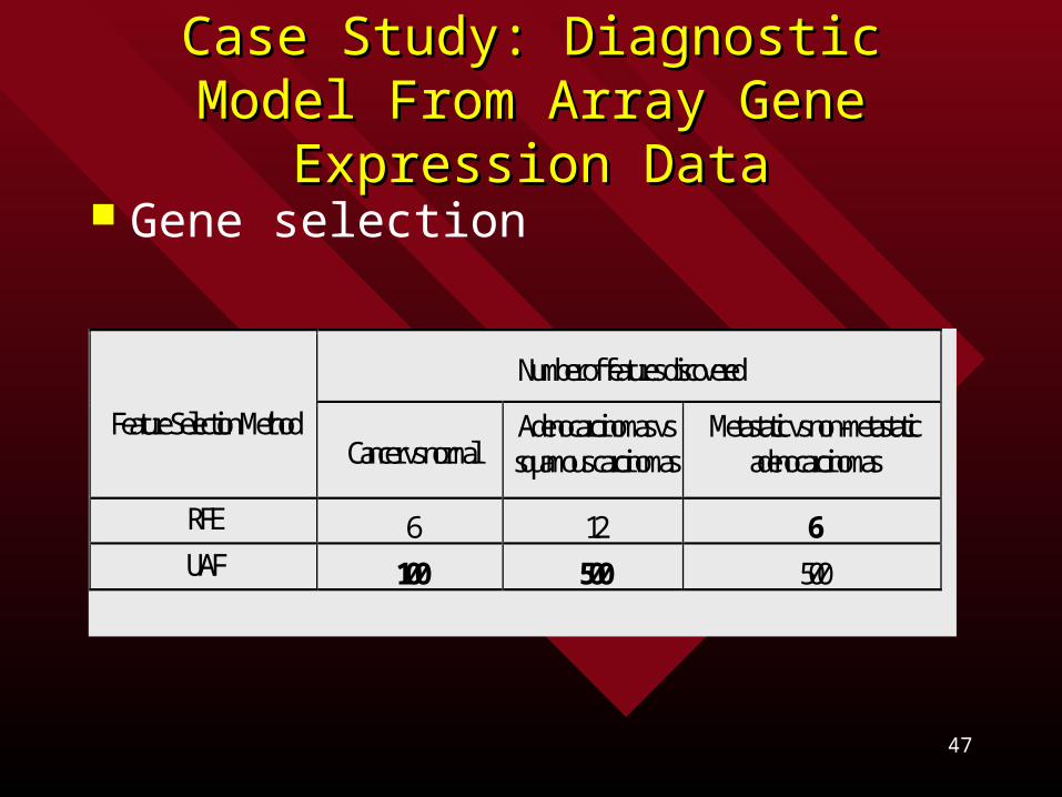
Gene selection
Number of features discovered
Feature Selection Method Cancer vs normal
Adenocarcinomas vs squamous carcinomas
Metastatic vs non-metastatic adenocarcinomas
RFE 6 12 6 UAF 100 500 500
48
Case Study: Diagnostic Model From Case Study: Diagnostic Model From Array Gene Expression DataArray Gene Expression Data
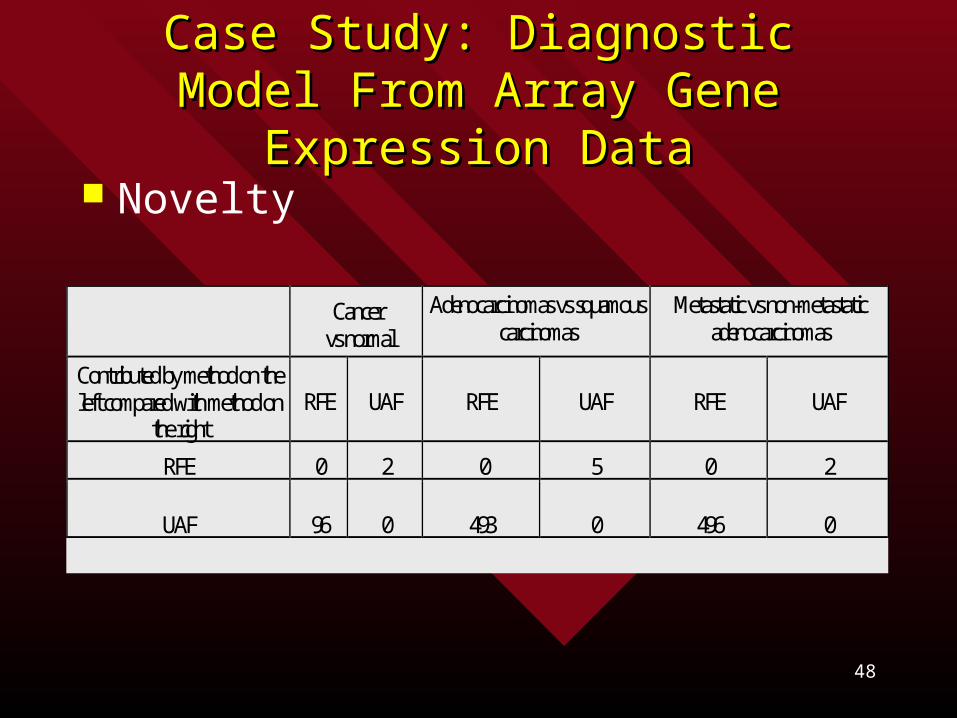
Novelty
Cancer
vs normal
Adenocarcinomas vs squamous carcinomas
Metastatic vs non-metastatic adenocarcinomas
Contributed by method on the left compared with method on
the right RFE UAF RFE UAF RFE UAF
RFE 0 2 0 5 0 2
UAF 96 0 493 0 496 0

49
Case Study: Diagnostic Model From Case Study: Diagnostic Model From Array Gene Expression DataArray Gene Expression Data
A more detailed look:– Specific Aim 3: “Study how aspects of experimental design
(including data set, measured genes, sample size, cross-validation methodology) determine the performance and stability of several machine learning (classifier and feature selection) methods used in the experiments”.

50
Case Study: Diagnostic Model From Case Study: Diagnostic Model From Array Gene Expression DataArray Gene Expression Data
Overfitting: we replace actual gene measurements by random values in the same range (while retaining the outcome variable values).
Target class rarity: we contrast performance in tasks with rare vs non-rare categories.
Sample size: we use samples from the set {40,80,120,160, 203} range (as applicable in each task).
Predictor info redundancy: we replace the full set of predictors by random subsets with sizes in the set {500, 1000, 5000, 12600}.

51
Case Study: Diagnostic Model From Case Study: Diagnostic Model From Array Gene Expression DataArray Gene Expression Data
Train-test split ratio: we use train-test ratios from the set {80/20, 60/40, 40/60} (for tasks II and III, while for task I modified ratios were used due to small number of positives, see Figure 1).
Cross-validated fold construction: we construct n-fold cross-validation samples retaining the proportion of the rarer target category to the more frequent one in folds with smaller sample, or, alternatively we ensure that all rare instances are included in the union of test sets (to maximize use of rare-case instances).
Classifier type: Kernel vs non-kernel and linear vs non-linear classifiers are contrasted. Specifically we compare linear and non-linear SVMs (a prototypical kernel method) to each other and to KNN (a robust and well-studied non-kernel classifier and density estimator).

52
Case Study: Diagnostic Model From Array Gene Case Study: Diagnostic Model From Array Gene Expression Data Expression Data Random gene values Random gene values
Classifier
Task I. Metastatic (7) –Nonmetastatic (132)
Task II. Cancer (186)-Normal (17)
Task III. Adenocarcinomas (139) - Squamous carcinomas (21)
SVMs 0.584 (139 cases) 0.583 (203 cases) 0.572 (160 cases) KNN 0.581 (139 cases) 0.522 (203 cases) 0.559 (160 cases)
Classifier
Task I. Metastatic (7) –Nonmetastatic (132)
Task II. Cancer (186)-Normal (17)
Task III. Adenocarcinomas (139) - Squamous carcinomas (21)
SVMs 0.968 (139 cases) 0.996 (203 cases) 0.990 (160 cases) KNN 0.926 (139 cases) 0.981 (203 cases) 0.976 (160 cases)

53
Case Study: Diagnostic Model From Array Gene Case Study: Diagnostic Model From Array Gene Expression Data Expression Data varying sample size varying sample size
Classifier
Task I. Metastatic (7) –Nonmetastatic (132)
Task II. Cancer (186)-Normal (17)
Task III. Adenocarcinomas (139) - Squamous carcinomas (21)
SVMs 0.982 (40 cases) , 0,982 (80 cases), 0.969 (120 cases)
1 (40 cases) , 1 (80 cases), 1 (120 cases), 0.995 (160 cases)
0.981 (40 cases) , 0.988 (80 cases), 0.980 (120 cases)
KNN 0.893 (40 cases) , 0,832 (80 cases), 0.925 (120 cases)
1 (40 cases) , 1 (80 cases), 0.993 (120 cases), 0.970 (160 cases)
0.916 (40 cases) , 0.960 (80 cases), 0.965 (120 cases)
Classifier
Task I. Metastatic (7) –Nonmetastatic (132)
Task II. Cancer (186)-Normal (17)
Task III. Adenocarcinomas (139) - Squamous carcinomas (21)
SVMs 0.968 (139 cases) 0.996 (203 cases) 0.990 (160 cases) KNN 0.926 (139 cases) 0.981 (203 cases) 0.976 (160 cases)

54
Case Study: Diagnostic Model From Array Gene Case Study: Diagnostic Model From Array Gene Expression Data Expression Data Random gene selection Random gene selection
Classifier
Task I. Metastatic (7) –Nonmetastatic (132)
Task II. Cancer (186)-Normal (17)
Task III. Adenocarcinomas (139) - Squamous carcinomas (21)
SVMs 0.944 (500 genes), 0.948 (1000 genes), 0.956 (5000 genes)
0.991 (500 genes), 0.989 (1000 genes), 0.995 (5000 genes)
0.982 (500 genes), 0.987 (1000 genes), 0.990 (5000 genes)
KNN 0.893 (500 genes), 0.893 (1000 genes), 0.941 (5000 genes)
0.959 (500 genes), 0.961 (1000 genes), 0.984 (5000 genes)
0.928 (500 genes), 0.955 (1000 genes), 0.965 (5000 genes)
Classifier
Task I. Metastatic (7) –Nonmetastatic (132)
Task II. Cancer (186)-Normal (17)
Task III. Adenocarcinomas (139) - Squamous carcinomas (21)
SVMs 0.968 (139 cases) 0.996 (203 cases) 0.990 (160 cases) KNN 0.926 (139 cases) 0.981 (203 cases) 0.976 (160 cases)

55
Case Study: Diagnostic Model From Array Gene Case Study: Diagnostic Model From Array Gene Expression Data Expression Data Split ratio Split ratio
Classifier
Task I. Metastatic (7) –Nonmetastatic (132)
Task II. Cancer (186)-Normal (17)
Task III. Adenocarcinomas (139) - Squamous carcinomas (21)
SVMs 0.915 (30/70), 0.938 (43/57), 0.954 (57/43), 0.962 (70/30), 0.968 (85/15)
0.997 (40/60), 0.996 (60/40), 0.996 (80/20)
0.989 (40/60), 0.990 (60/40), 0.990 (80/20)
KNN 0.782 (30/70), 0.833 (43/57), 0.866 (57/43), 0.901 (70/30), 0.990 (85/15)
0.960 (40/60), 0.962 (60/40), 0.976 (80/20)
0.960 (40/60), 0.962 (60/40), 0.976 (80/20)
Classifier
Task I. Metastatic (7) –Nonmetastatic (132)
Task II. Cancer (186)-Normal (17)
Task III. Adenocarcinomas (139) - Squamous carcinomas (21)
SVMs 0.968 (139 cases) 0.996 (203 cases) 0.990 (160 cases) KNN 0.926 (139 cases) 0.981 (203 cases) 0.976 (160 cases)
56
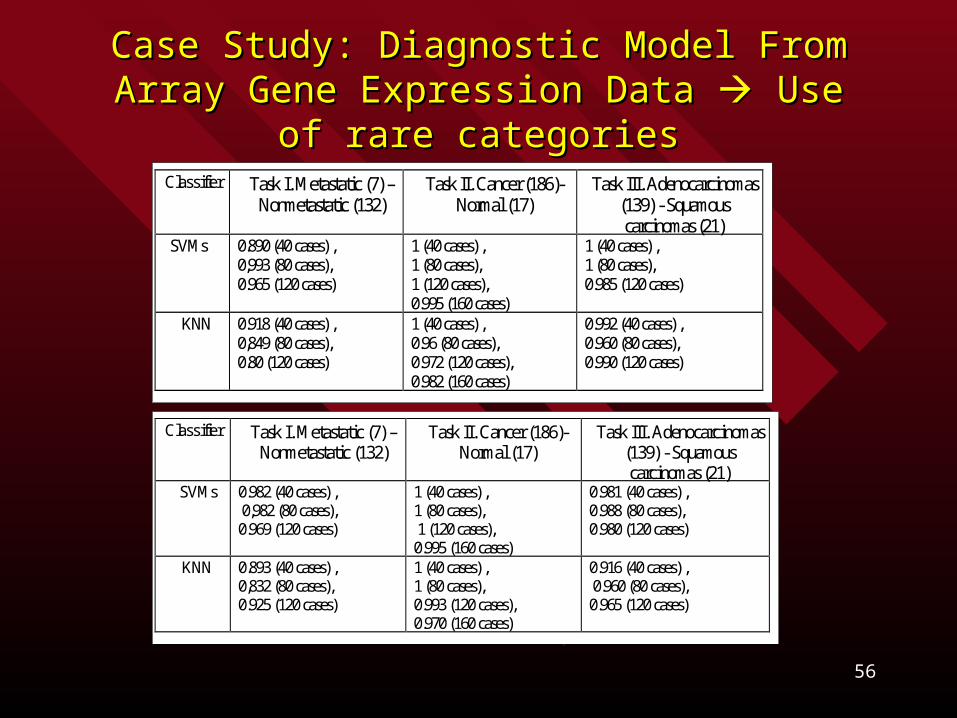
Case Study: Diagnostic Model From Array Gene Case Study: Diagnostic Model From Array Gene Expression Data Expression Data Use of rare categories Use of rare categories
Classifier
Task I. Metastatic (7) –Nonmetastatic (132)
Task II. Cancer (186)-Normal (17)
Task III. Adenocarcinomas (139) - Squamous carcinomas (21)
SVMs 0.890 (40 cases) , 0,993 (80 cases), 0.965 (120 cases)
1 (40 cases) , 1 (80 cases), 1 (120 cases), 0.995 (160 cases)
1 (40 cases) , 1 (80 cases), 0.985 (120 cases)
KNN 0.918 (40 cases) , 0,849 (80 cases), 0.80 (120 cases)
1 (40 cases) , 0.96 (80 cases), 0.972 (120 cases), 0.982 (160 cases)
0.992 (40 cases) , 0.960 (80 cases), 0.990 (120 cases)
Classifier
Task I. Metastatic (7) –
Nonmetastatic (132) Task II. Cancer (186)-
Normal (17) Task III. Adenocarcinomas
(139) - Squamous carcinomas (21)
SVMs 0.982 (40 cases) , 0,982 (80 cases), 0.969 (120 cases)
1 (40 cases) , 1 (80 cases), 1 (120 cases), 0.995 (160 cases)
0.981 (40 cases) , 0.988 (80 cases), 0.980 (120 cases)
KNN 0.893 (40 cases) , 0,832 (80 cases), 0.925 (120 cases)
1 (40 cases) , 1 (80 cases), 0.993 (120 cases), 0.970 (160 cases)
0.916 (40 cases) , 0.960 (80 cases), 0.965 (120 cases)
57
Case Study: Diagnostic Model From Case Study: Diagnostic Model From Array Gene Expression DataArray Gene Expression Data
We have recently completed an extensive analysis of all multi-category gene expression-based cancer datasets in the public domain. The analysis spans >75 cancer types and >1,000 patients in 12 datasets.
On the basis of this study we have created a tool that automatically analyzes data to create diagnostic systems and identify biomarker candidates using a variety of techniques.
The present incarnation of the tool is oriented toward the computer-savvy researcher; a more biologist-friendly web-accessible version is under development.
58
Case Study: Diagnostic Model From Case Study: Diagnostic Model From Array Gene Expression DataArray Gene Expression Data
Questions:– What would you do differently?– How to interpret the biological significance of
the selected genes?– What is wrong with having so many and robust
good classification models?– Why do we have so many good models?

59
Case Study: Diagnostic Model From Case Study: Diagnostic Model From Array Gene Expression DataArray Gene Expression Data
MC-SVM (alpha) Demonstration

60
Case Study: Imputation for Machine Learning Models For Lung Cancer
Classification Using Array Comparative Genomic Hybridization
C.F. Aliferis M.D., Ph.D., D. Hardin Ph.D., P. P. Massion M.D.
AMIA 2002

61
Case Study: A Protocol to Address the Case Study: A Protocol to Address the Missing Values ProblemMissing Values Problem
Context:– Array comparative genomic hybridization (array CGH): recently
introduced technology that measures gene copy number changes of hundreds of genes in a single experiment. Gene copy number changes (deletion, amplification) are often characteristic of disease and cancer in particular.
– aCGH as been shown in studies published during the last years that it enables development of powerful classification models, facilitate selection of genes for array design, and identification of likely oncogenes in a variety of cancers (e.g., esophageal, renal, head/neck, lymphomas, breast, and glioblastomas).
– Interestingly a recent study (Fritz et al. June 2002) has shown that aCGH enables better classification of liposarcoma differentiation than gene expression information.
62
Case Study: A Protocol to Address the Case Study: A Protocol to Address the Missing Values ProblemMissing Values Problem
Context:– While significant experience has been gathered so far in the
application of various machine learning/data mining approaches to explore development of diagnostic/classification models with gene expression Microarray Data for lung cancer and of aCGH in a variety of cancers, little was known about the feasibility of using machine learning methods with aCGH data to create such models.
– In this study we conducted such an experiment for the classification of non-small Lung Cancers (NSCLCs) as squamus carcinomas (SqCa) or adenocarcinomas (AdCa)). A related goal was to compare several machine learning methods in this learning task.

63
Case Study: A Protocol to Address the Case Study: A Protocol to Address the Missing Values ProblemMissing Values Problem
Context:– DNA from tumors of 37 patients (21 squamous carcinomas,
(SqCa) and 16 adenocarcinomas (AdCa)) were extracted after microdissection and hybridized onto a 452 BAC clone array (printed in quadruplicate) carrying genes of potential importance in cancer.
– aCGH is a technology in formative stages of development. As a result a high percentage of missing values was observed in most gene measurements.

64
We decided to create a protocol for gene inclusion/exclusion for analysis on the basis of three criteria: – (a) percentage of missing values,
– (b) a priori importance of a gene (based on known functional role in pathways that are implicated in carcinogenesis such as the PI3-kinase pathway), and
– (c) whether the existence of missing values was statistically significantly associated with the class to be predicted (at the 0.05 level and determined by a G2 test).
Case Study: A Protocol to Address the Case Study: A Protocol to Address the Missing Values ProblemMissing Values Problem

65
1. For each gene Gi compute an indicator variable MGi s.t. MGi is 1 in cases where Gi is missing , and 0 in cases where Gi
was observed2. Compute the association of MGi to the class variable C,
assoc(MGi , C) for every i. (C takes values in {SqCa, AdCa})
3. Accept a set of important genes I4. if assoc(MGi , C) is statistically significant then reject
gene Gi
else if Gi I then accept Gi else if fraction of missing values of Gi is >15% then reject Gi else accept Gi
388 variables were selected according to this protocol and were imputed before analysis.
Case Study: A Protocol to Address the Case Study: A Protocol to Address the Missing Values ProblemMissing Values Problem

66
K-Nearest Neighbors (KNN) method for imputation– for each instance of a gene that had a missing value the case closest to the case
containing that missing value (i.e., the closest neighbor) that did have an observed value for the gene was found using Euclidean Distance (ED). That value was substituted for the missing one.
– To compute distances between cases with missing values, if one of the two corresponding gene measurements was missing, the mean of the observed values for this gene across all cases was used to compute the ED component.
– When both values were missing, the mean observed difference was used for the ED component.
The above procedure because it is non-parametric and multivariate. More naïve approaches (such as imputing with the mean or with a random
value from the observed distribution for the gene) typically produced uniformly worse models.
A variant of the above method iterates the KNN imputation until convergence is attained.
Case Study: A Protocol to Address the Case Study: A Protocol to Address the Missing Values ProblemMissing Values Problem

67
Important note: Clear understanding of what types of missing values we have and what are the mechanisms that generate them is required and sometimes translates into ability to effectively replace missing values as well as avoid serious biases.
Example types of missing values:– Value is not produced by device or respondent etc.– Value was produced but not entered in the study database– Value was produced and entered but is deemed invalid on substantive
grounds– Value was produced and entered but was subsequently corrupted due to
transmission/storage or data conversion operations, etc. Example where knowing process that generates missing values may be
sufficient to fill them in: physician does not measure a lab value (say x-ray) because an equivalent or more informative test has been conducted (e.g., MRI) or because it is physiologically impossible for a change to have occurred from last measurement, etc.
Case Study: A Protocol to Address the Case Study: A Protocol to Address the Missing Values ProblemMissing Values Problem