3 Weighted Networks – The Perceptron - Freie Universität · 2008-01-11 · 3 Weighted Networks...

R. Rojas: Neural Networks, Springer-Verlag, Berlin, 1996

3

Weighted Networks – The Perceptron

3.1 Perceptrons and parallel processing

In the previous chapter we arrived at the conclusion that McCulloch–Pittsunits can be used to build networks capable of computing any logical functionand of simulating any finite automaton. From the biological point of view,however, the types of network that can be built are not very relevant. Thecomputing units are too similar to conventional logic gates and the networkmust be completely specified before it can be used. There are no free param-eters which could be adjusted to suit different problems. Learning can onlybe implemented by modifying the connection pattern of the network and thethresholds of the units, but this is necessarily more complex than just adjust-ing numerical parameters. For that reason, we turn our attention to weightednetworks and consider their most relevant properties. In the last section of thischapter we show that simple weighted networks can provide a computationalmodel for regular neuronal structures in the nervous system.

3.1.1 Perceptrons as weighted threshold elements

In 1958 Frank Rosenblatt, an American psychologist, proposed the percep-tron, a more general computational model than McCulloch–Pitts units. Theessential innovation was the introduction of numerical weights and a spe-cial interconnection pattern. In the original Rosenblatt model the computingunits are threshold elements and the connectivity is determined stochastically.Learning takes place by adapting the weights of the network with a numericalalgorithm. Rosenblatt’s model was refined and perfected in the 1960s and itscomputational properties were carefully analyzed by Minsky and Papert [312].In the following, Rosenblatt’s model will be called the classical perceptron andthe model analyzed by Minsky and Papert the perceptron.

The classical perceptron is in fact a whole network for the solution of cer-tain pattern recognition problems. In Figure 3.1 a projection surface called the

R. Rojas: Neural Networks, Springer-Verlag, Berlin, 1996R. Rojas: Neural Networks, Springer-Verlag, Berlin, 1996


56 3 Weighted Networks – The Perceptron

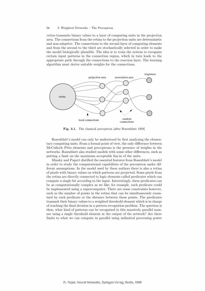
retina transmits binary values to a layer of computing units in the projectionarea. The connections from the retina to the projection units are deterministicand non-adaptive. The connections to the second layer of computing elementsand from the second to the third are stochastically selected in order to makethe model biologically plausible. The idea is to train the system to recognizecertain input patterns in the connection region, which in turn leads to theappropriate path through the connections to the reaction layer. The learningalgorithm must derive suitable weights for the connections.

retina

projection area association arearesponses

randomconnections

local connections

Fig. 3.1. The classical perceptron [after Rosenblatt 1958]

Rosenblatt’s model can only be understood by first analyzing the elemen-tary computing units. From a formal point of view, the only difference betweenMcCulloch–Pitts elements and perceptrons is the presence of weights in thenetworks. Rosenblatt also studied models with some other differences, such asputting a limit on the maximum acceptable fan-in of the units.

Minsky and Papert distilled the essential features from Rosenblatt’s modelin order to study the computational capabilities of the perceptron under dif-ferent assumptions. In the model used by these authors there is also a retinaof pixels with binary values on which patterns are projected. Some pixels fromthe retina are directly connected to logic elements called predicates which cancompute a single bit according to the input. Interestingly, these predicates canbe as computationally complex as we like; for example, each predicate couldbe implemented using a supercomputer. There are some constraints however,such as the number of points in the retina that can be simultaneously exam-ined by each predicate or the distance between those points. The predicatestransmit their binary values to a weighted threshold element which is in chargeof reaching the final decision in a pattern recognition problem. The question isthen, what kind of patterns can be recognized in this massively parallel man-ner using a single threshold element at the output of the network? Are therelimits to what we can compute in parallel using unlimited processing power



3.1 Perceptrons and parallel processing 57

for each predicate, when each predicate cannot itself look at the whole retina?The answer to this problem in some ways resembles the speedup problem inparallel processing, in which we ask what percentage of a computational taskcan be parallelized and what percentage is inherently sequential.

w1

w2

w3

w4

P1

P2

P3

P4

θ

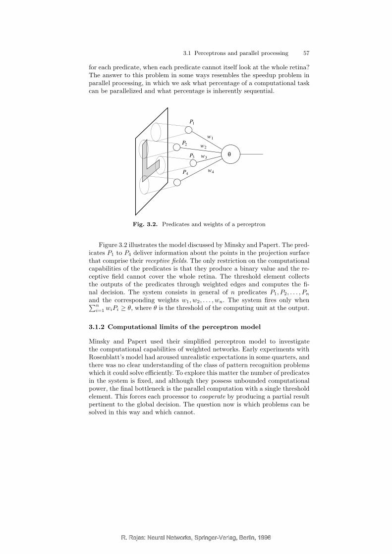
Fig. 3.2. Predicates and weights of a perceptron

Figure 3.2 illustrates the model discussed by Minsky and Papert. The pred-icates P1 to P4 deliver information about the points in the projection surfacethat comprise their receptive fields. The only restriction on the computationalcapabilities of the predicates is that they produce a binary value and the re-ceptive field cannot cover the whole retina. The threshold element collectsthe outputs of the predicates through weighted edges and computes the fi-nal decision. The system consists in general of n predicates P1, P2, . . . , Pn

and the corresponding weights w1, w2, . . . , wn. The system fires only when∑n

i=1 wiPi ≥ θ, where θ is the threshold of the computing unit at the output.

3.1.2 Computational limits of the perceptron model

Minsky and Papert used their simplified perceptron model to investigatethe computational capabilities of weighted networks. Early experiments withRosenblatt’s model had aroused unrealistic expectations in some quarters, andthere was no clear understanding of the class of pattern recognition problemswhich it could solve efficiently. To explore this matter the number of predicatesin the system is fixed, and although they possess unbounded computationalpower, the final bottleneck is the parallel computation with a single thresholdelement. This forces each processor to cooperate by producing a partial resultpertinent to the global decision. The question now is which problems can besolved in this way and which cannot.




The system considered by Minsky and Papert at first appears to be astrong simplification of parallel decision processes, but it contains some of themost important elements differentiating between sequential and parallel pro-cessing. It is known that when some algorithms are parallelized, an irreduciblesequential component sometimes limits the maximum achievable speedup. Themathematical relation between speedup and irreducible sequential portion ofan algorithm is known as Amdahl’s law [187]. In the model considered abovethe central question is, are there pattern recognition problems in which weare forced to analyze sequentially the output of the predicates associated witheach receptive field or not? Minsky and Papert showed that problems of thiskind do indeed exist which cannot be solved by a single perceptron acting asthe last decision unit.

The limits imposed on the receptive fields of the predicates are based onrealistic assumptions. The predicates are fixed in advance and the patternrecognition problem can be made arbitrarily large (by expanding the retina).According to the number of points and their connections to the predicates,Minsky and Papert differentiated between

• Diameter limited perceptrons: the receptive field of each predicate has alimited diameter.

• Perceptrons of limited order: each receptive field can only contain up to acertain maximum number of points.

• Stochastic perceptrons: each receptive field consists of a number of ran-domly chosen points

Some patterns are more difficult to identify than others and this struc-tural classification of perceptrons is a first attempt at defining something likecomplexity classes for pattern recognition. Connectedness is an example of aproperty that cannot be recognized by constrained systems.

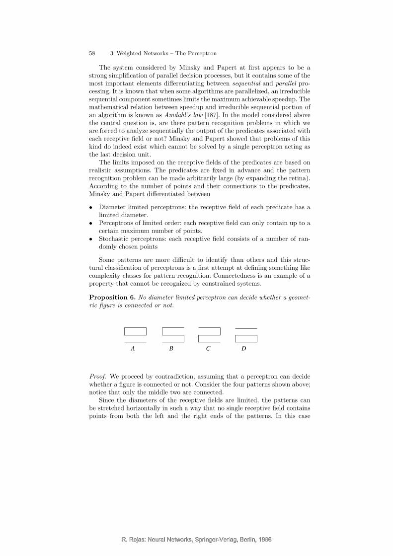
Proposition 6. No diameter limited perceptron can decide whether a geomet-ric figure is connected or not.

A B C D

Proof. We proceed by contradiction, assuming that a perceptron can decidewhether a figure is connected or not. Consider the four patterns shown above;notice that only the middle two are connected.

Since the diameters of the receptive fields are limited, the patterns canbe stretched horizontally in such a way that no single receptive field containspoints from both the left and the right ends of the patterns. In this case



3.1 Perceptrons and parallel processing 59

we have three different groups of predicates: the first group consists of thosepredicates whose receptive fields contain points from the left side of a pattern.Predicates of the second group are those whose receptive fields cover the rightside of a pattern. All other predicates belong to the third group. In Figure 3.3the receptive fields of the predicates are represented by circles.

group 1 group 3 group 2

Fig. 3.3. Receptive fields of predicates

All predicates are connected to a threshold element through weighted edgeswhich we denote by the letter w with an index. The threshold element decideswhether a figure is connected or not by performing the computation

S =∑

Pi∈group 1

w1iPi +∑

Pi∈group 2

w2iPi +∑

Pi∈group 3

w3iPi − θ ≥ 0.

If S is positive the figure is recognized as connected, as is the case, for example,in Figure 3.3.

If the disconnected pattern A is analyzed, then we should have S < 0.Pattern A can be transformed into pattern B without affecting the output ofthe predicates of group 3, which do not recognize the difference since theirreceptive fields do not cover the sides of the figures. The predicates of group2 adjust their outputs by ∆2S so that now

S +∆2S ≥ 0⇒ ∆2S ≥ −S.

If pattern A is transformed into pattern C, the predicates of group 1 adjusttheir outputs so that the threshold element receives a net excitation, i.e.,

S +∆1S ≥ 0⇒ ∆1S ≥ −S.

However, if pattern A is transformed into pattern D, the predicates of group1 cannot distinguish this case from the one for figure C and the predicatesof group 2 cannot distinguish this case from the one for figure B. Since thepredicates of group 3 do not change their output we have




∆S = ∆2S +∆1S ≥ −2S,

and from thisS +∆S ≥ −S > 0.

The value of the new sum can only be positive and the whole system classifiesfigure D as connected. Since this is a contradiction, such a system cannotexist. 2

Proposition 6 states only that the connectedness of a figure is a globalproperty which cannot be decided locally. If no predicate has access to thewhole figure, then the only alternative is to process the outputs of the predi-cates sequentially.

There are some other difficult problems for perceptrons. They cannot de-cide, for example, whether a set of points contains an even or an odd numberof elements when the receptive fields cover only a limited number of points.

3.2 Implementation of logical functions

In the previous chapter we discussed the synthesis of Boolean functions usingMcCulloch–Pitts networks. Weighted networks can achieve the same resultswith fewer threshold gates, but the issue now is which functions can be im-plemented using a single unit.

3.2.1 Geometric interpretation

In each of the previous sections a threshold element was associated with awhole set of predicates or a network of computing elements. From now on, wewill deal with perceptrons as isolated threshold elements which compute theiroutput without delay.

Definition 1. A simple perceptron is a computing unit with threshold θ which,when receiving the n real inputs x1, x2, . . . , xn through edges with the associ-ated weights w1, w2, . . . , wn, outputs 1 if the inequality

∑ni=1 wixi ≥ θ holds

and otherwise 0.

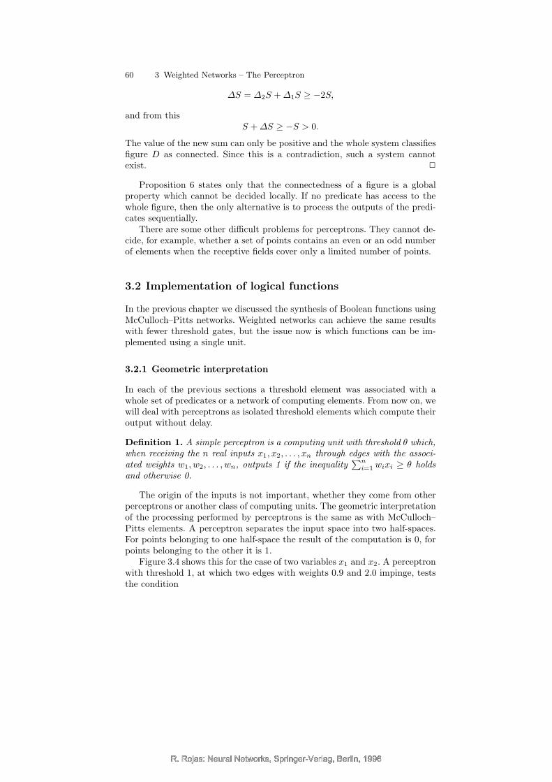
The origin of the inputs is not important, whether they come from otherperceptrons or another class of computing units. The geometric interpretationof the processing performed by perceptrons is the same as with McCulloch–Pitts elements. A perceptron separates the input space into two half-spaces.For points belonging to one half-space the result of the computation is 0, forpoints belonging to the other it is 1.

Figure 3.4 shows this for the case of two variables x1 and x2. A perceptronwith threshold 1, at which two edges with weights 0.9 and 2.0 impinge, teststhe condition



3.2 Implementation of logical functions 61

0. 9x1 + 2x2 ≥ 1

0. 9x1 + 2x2 < 1

x1

x2

Fig. 3.4. Separation of input space with a perceptron

0.9x1 + 2x2 ≥ 1.

It is possible to generate arbitrary separations of input space by adjusting theparameters of this example.

In many cases it is more convenient to deal with perceptrons of thresh-old zero only. This corresponds to linear separations which are forced to gothrough the origin of the input space. The two perceptrons in Figure 3.5 areequivalent. The threshold of the perceptron to the left has been convertedinto the weight −θ of an additional input channel connected to the constant1. This extra weight connected to a constant is called the bias of the element.

1

0

w1

wn

−θ

w1

wn

x1 x1

xn xn

θ ⇒...

...

Fig. 3.5. A perceptron with a bias

Most learning algorithms can be stated more concisely by transformingthresholds into biases. The input vector (x1, x2, . . . , xn) must be extended withan additional 1 and the resulting (n+1)-dimensional vector (x1, x2, . . . , xn, 1)is called the extended input vector. The extended weight vector associatedwith this perceptron is (w1, . . . , wn, wn+1), whereby wn+1 = −θ.




3.2.2 The XOR problem

We can now deal with the problem of determining which logical functions canbe implemented with a single perceptron. A perceptron network is capableof computing any logical function, since perceptrons are even more powerfulthan unweighted McCulloch–Pitts elements. If we reduce the network to asingle element, which functions are still computable?

Taking the functions of two variables as an example we can gain someinsight into this problem. Table 3.1 shows all 16 possible Boolean functionsof two variables f0 to f15. Each column fi shows the value of the function foreach combination of the two variables x1 and x2. The function f0, for example,is the zero function whereas f14 is the OR-function.

Table 3.1. The 16 Boolean functions of two variables

x1 x2 f0 f1 f2 f3 f4 f5 f6 f7 f8 f9 f10 f11 f12 f13 f14 f15

0 0 0 1 0 1 0 1 0 1 0 1 0 1 0 1 0 10 1 0 0 1 1 0 0 1 1 0 0 1 1 0 0 1 11 0 0 0 0 0 1 1 1 1 0 0 0 0 1 1 1 11 1 0 0 0 0 0 0 0 0 1 1 1 1 1 1 1 1

Perceptron-computable functions are those for which the points whosefunction value is 0 can be separated from the points whose function value is1 using a line. Figure 3.6 shows two possible separations to compute the ORand the AND functions.

1 1

10

0

0 0

1

OR AND

Fig. 3.6. Separations of input space corresponding to OR and AND

It is clear that two of the functions in the table cannot be computed inthis way. They are the function XOR and identity (f6 and f9). It is intuitivelyevident that no line can produce the necessary separation of the input space.This can also be shown analytically.



3.3 Linearly separable functions 63

Let w1 and w2 be the weights of a perceptron with two inputs, and θ itsthreshold. If the perceptron computes the XOR function the following fourinequalities must be fulfilled:

x1 = 0 x2 = 0 w1x1 + w2x2 = 0 ⇒ 0 < θx1 = 1 x2 = 0 w1x1 + w2x2 = w1 ⇒ w1 ≥ θx1 = 0 x2 = 1 w1x1 + w2x2 = w2 ⇒ w2 ≥ θx1 = 1 x2 = 1 w1x1 + w2x2 = w1 + w2 ⇒ w1 + w2 < θ

Since θ is positive, according to the first inequality, w1 and w2 are positivetoo, according to the second and third inequalities. Therefore the inequalityw1 + w2 < θ cannot be true. This contradiction implies that no perceptroncapable of computing the XOR function exists. An analogous proof holds forthe function f9.

3.3 Linearly separable functions

The example of the logical functions of two variables shows that the problemof perceptron computability must be discussed in more detail. In this sectionwe provide the necessary tools to deal more effectively with functions of narguments.

3.3.1 Linear separability

We can deduce from our experience with the XOR function that many otherlogical functions of several arguments must exist which cannot be computedwith a threshold element. This fact has to do with the geometry of the n-dimensional hypercube whose vertices represent the combination of logic val-ues of the arguments. Each logical function separates the vertices into twoclasses. If the points whose function value is 1 cannot be separated witha linear cut from the points whose function value is 0, the function is notperceptron-computable. The following two definitions give this problem amore general setting.

Definition 2. Two sets of points A and B in an n-dimensional space arecalled linearly separable if n + 1 real numbers w1, . . . , wn+1 exist, such thatevery point (x1, x2, . . . , xn) ∈ A satisfies

∑ni=1 wixi ≥ wn+1 and every point

(x1, x2, . . . , xn) ∈ B satisfies∑n

i=1 wixi < wn+1

Since a perceptron can only compute linearly separable functions, an inter-esting question is how many linearly separable functions of n binary argumentsthere are. When n = 2, 14 out of the 16 possible Boolean functions are lin-early separable. When n = 3, 104 out of 256 and when n = 4, 1882 out of65536 possible functions are linearly separable. Although there has been ex-tensive research on linearly separable functions in recent years, no formula for




expressing the number of linearly separable functions as a function of n hasyet been found. However we will provide some upper bounds for this numberin the following chapters.

3.3.2 Duality of input space and weight space

The computation performed by a perceptron can be visualized as a linear sep-aration of input space. However, when trying to find the appropriate weightsfor a perceptron, the search process can be better visualized in weight space.When m real weights must be determined, the search space is the whole ofIRm.

x1

x2

w1

w2

•

•

− θ = w3x3

Fig. 3.7. Illustration of the duality of input and weight space

For a perceptron with n input lines, finding the appropriate linear sep-aration amounts to finding n + 1 free parameters (n weights and the bias).These n+1 parameters represent a point in (n+1)-dimensional weight space.Each time we pick one point in weight space we are choosing one combina-tion of weights and a specific linear separation of input space. This meansthat every point in (n + 1)-dimensional weight space can be associated witha hyperplane in (n + 1)-dimensional extended input space. Figure 3.7 showsan example. Each combination of three weights, w1, w2, w3, which representa point in weight space, defines a separation of input space with the planew1x1 + w2x2 + w3x3 = 0.

There is the same kind of relation in the inverse direction, from input toweight space. If we want the point x1, x2, x3 to be located in the positivehalf-space defined by a plane, we need to determine the appropriate weightsw1, w2 and w3. The inequality

w1x1 + w2x2 + w3x3 ≥ 0

must hold. However this inequality defines a linear separation of weight space,that is, the point (x1, x2, x3) defines a cutting plane in weight space. Points inone space are mapped to planes in the other and vice versa. This complemen-tary relation is called duality. Input and weight space are dual spaces and we



3.3 Linearly separable functions 65

can visualize the computations done by perceptrons and learning algorithmsin any one of them. We will switch from one visualization to the other asnecessary or convenient.

3.3.3 The error function in weight space

Given two sets of patterns which must be separated by a perceptron, a learn-ing algorithm should automatically find the weights and threshold necessaryfor the solution of the problem. The perceptron learning algorithm can accom-plish this for threshold units. Although proposed by Rosenblatt it was alreadyknown in another context [10].

Assume that the set A of input vectors in n-dimensional space must beseparated from the set B of input vectors in such a way that a perceptroncomputes the binary function fw with fw(x) = 1 for x ∈ A and fw(x) = 0for x ∈ B. The binary function fw depends on the set w of weights andthreshold. The error function is the number of false classifications obtainedusing the weight vector w. It can be defined as:

E(w) =∑

x∈A

(1 − fw(x)) +∑

x∈B

fw(x).

This is a function defined over all of weight space and the aim of perceptronlearning is to minimize it. Since E(w) is positive or zero, we want to reach theglobal minimum where E(w) = 0. This will be done by starting with a randomweight vector w, and then searching in weight space a better alternative, inan attempt to reduce the error function E(w) at each step.

3.3.4 General decision curves

A perceptron makes a decision based on a linear separation of the input space.This reduces the kinds of problem solvable with a single perceptron. Moregeneral separations of input space can help to deal with other kinds of problemunsolvable with a single threshold unit. Assume that a single computing unitcan produce the separation shown in Figure 3.8. Such a separation of the inputspace into two regions would allow the computation of the XOR function witha single unit. Functions used to discriminate between regions of input spaceare called decision curves [329]. Some of the decision curves which have beenstudied are polynomials and splines.

In statistical pattern recognition problems we assume that the patterns tobe recognized are grouped in clusters in input space. Using a combination ofdecision curves we try to isolate one cluster from the others. One alternativeis combining several perceptrons to isolate a convex region of space. Otheralternatives which have been studied are, for example, so-called Sigma-Piunits which, for a given input x1, x2, . . . , xn, compute the sum of all or somepartial products of the form xixj [384].




1

1

0

0

Fig. 3.8. Non-linear separation of input space

In the general case we want to distinguish between regions of space. Aneural network must learn to identify these regions and to associate themwith the correct response. The main problem is determining whether the freeparameters of these decision regions can be found using a learning algorithm.In the next chapter we show that it is always possible to find these freeparameters for linear decision curves, if the patterns to be classified are indeedlinearly separable. Finding learning algorithms for other kinds of decisioncurves is an important research topic not dealt with here [45, 4].

3.4 Applications and biological analogy

The appeal of the perceptron model is grounded on its simplicity and thewide range of applications that it has found. As we show in this section,weighted threshold elements can play an important role in image processingand computer vision.

3.4.1 Edge detection with perceptrons

A good example of the pattern recognition capabilities of perceptrons is edgedetection (Figure 3.9). Assume that a method of extracting the edges of afigure darker than the background (or the converse) is needed. Each pixel inthe figure is compared to its immediate neighbors and in the case where thepixel is black and one of its neighbors white, it will be classified as part ofan edge. This can be programmed sequentially in a computer, but since thedecision about each point uses only local information, it is straightforward toimplement the strategy in parallel.

Assume that the figures to be processed are projected on a screen in whicheach pixel is connected to a perceptron, which also receives inputs from itsimmediate neighbors. Figure 3.10 shows the shape of the receptive field (aso-called Moore neighborhood) and the weights of the connections to theperceptron. The central point is weighted with 8 and the rest with −1. In thefield of image processing this is called a convolution operator, because it is



3.4 Applications and biological analogy 67

Fig. 3.9. Example of edge detection

used by centering it at each pixel of the image to produce a certain outputvalue for each pixel. The operator shown has a maximum at the center of thereceptive field and local minima at the periphery.

-1

-1

-1

-1

-1

-1

-1

8

-1

Fig. 3.10. Edge detection operator

Figure 3.11 shows the kind of interconnection we have in mind. A percep-tron is needed for each pixel. The interconnection pattern repeats for eachpixel in the projection lattice, taking care to treat the borders of the screendifferently. The weights are those given by the edge detection operator.

0.5

Fig. 3.11. Connection of a perceptron to the projection grid

For each pattern projected onto the screen, the weighted input is com-pared to the threshold 0.5. When all points in the neighborhood are blackor all white, the total excitation is 0. In the situation shown below the totalexcitation is 5 and the point in the middle belongs to an edge.

There are many other operators for different uses, such as detecting hor-izontal or vertical lines or blurring or making a picture sharper. The size of




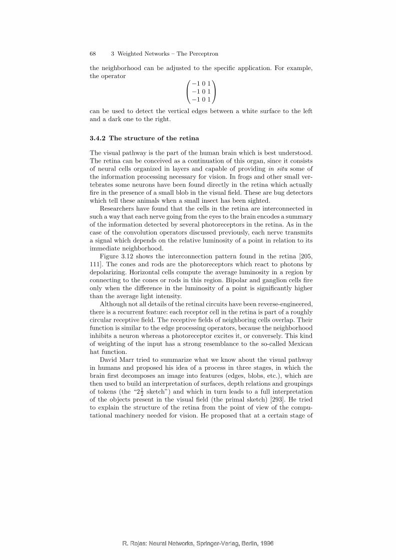
the neighborhood can be adjusted to the specific application. For example,the operator

−1 0 1−1 0 1−1 0 1

can be used to detect the vertical edges between a white surface to the leftand a dark one to the right.

3.4.2 The structure of the retina

The visual pathway is the part of the human brain which is best understood.The retina can be conceived as a continuation of this organ, since it consistsof neural cells organized in layers and capable of providing in situ some ofthe information processing necessary for vision. In frogs and other small ver-tebrates some neurons have been found directly in the retina which actuallyfire in the presence of a small blob in the visual field. These are bug detectorswhich tell these animals when a small insect has been sighted.

Researchers have found that the cells in the retina are interconnected insuch a way that each nerve going from the eyes to the brain encodes a summaryof the information detected by several photoreceptors in the retina. As in thecase of the convolution operators discussed previously, each nerve transmitsa signal which depends on the relative luminosity of a point in relation to itsimmediate neighborhood.

Figure 3.12 shows the interconnection pattern found in the retina [205,111]. The cones and rods are the photoreceptors which react to photons bydepolarizing. Horizontal cells compute the average luminosity in a region byconnecting to the cones or rods in this region. Bipolar and ganglion cells fireonly when the difference in the luminosity of a point is significantly higherthan the average light intensity.

Although not all details of the retinal circuits have been reverse-engineered,there is a recurrent feature: each receptor cell in the retina is part of a roughlycircular receptive field. The receptive fields of neighboring cells overlap. Theirfunction is similar to the edge processing operators, because the neighborhoodinhibits a neuron whereas a photoreceptor excites it, or conversely. This kindof weighting of the input has a strong resemblance to the so-called Mexicanhat function.

David Marr tried to summarize what we know about the visual pathwayin humans and proposed his idea of a process in three stages, in which thebrain first decomposes an image into features (edges, blobs, etc.), which arethen used to build an interpretation of surfaces, depth relations and groupingsof tokens (the “2 1

2 sketch”) and which in turn leads to a full interpretationof the objects present in the visual field (the primal sketch) [293]. He triedto explain the structure of the retina from the point of view of the compu-tational machinery needed for vision. He proposed that at a certain stage of




receptors

bipolar cells

ganglion cell

horizontal cells

Fig. 3.12. The interconnection pattern in the retina

pattern

weights

1

1

1

1

1111

1

–1

–1

–1

–1

–1

–1

–1

–1

–1

–1

–1

–1

–1

–1

–1

–1

Fig. 3.13. Feature detector for the pattern T

the computation the retina blurs an image and then extracts from it contrastinformation. Blurring an image can be done by averaging at each pixel thevalues of this pixel and its neighbors. A Gaussian distribution of weights canbe used for this purpose. Information about changes in darkness levels can be




extracted using the sum of the second derivatives of the illumination function,the so-called Laplace operator ∇2 = ∂2/∂x2 + ∂2/∂y2. The composition ofthe Laplace operator and a Gaussian blurring corresponds to the Mexican hatfunction. Processing of the image is done by computing the convolution of thediscrete version of the operator with the image. The 3× 3 discrete version ofthis operator is the edge detection operator which we used before. Differentlevels of blurring, and thus feature extraction at several different resolutionlevels, can be controlled by adjusting the size of the receptive fields of thecomputing units. It seems that the human visual pathway also exploits fea-ture detection at several resolution levels, which has led in turn to the idea ofusing several resolution layers for the computational analysis of images.

3.4.3 Pyramidal networks and the neocognitron

Single perceptrons can be thought of as feature detectors. Take the case ofFigure 3.13 in which a perceptron is defined with weights adequate for rec-ognizing the letter ‘T’ in which t pixels are black. If another ‘T’ is presented,in which one black pixel is missing, the excitation of the perceptron is t− 1.The same happens if one white pixel is transformed into a black one due tonoise, since the weights of the connections going from points that should bewhite are −1. If the threshold of the perceptron is set to t − 1, then thisperceptron will be capable of correctly classifying patterns with one noisypixel. By adjusting the threshold of the unit, 2, 3 or more noisy pixels can betolerated. Perceptrons thus compute the similarity of a pattern to the idealpattern they have been designed to identify, and the threshold is the minimalsimilarity that we require from the pattern. Note that since the weights ofthe perceptron are correlated with the pattern it recognizes, a simple way tovisualize the connections of a perceptron is to draw the pattern it identifiesin its receptive field. This technique will be used below.

The problem with this pattern recognition scheme is that it only worksif the patterns have been normalized in some way, that is, if they have beencentered in the window to which the perceptron connects and their size doesnot differ appreciably from the ideal pattern. Also, any kind of translationalshift will lead to ideal patterns no longer being recognized. The same happensin the case of rotations.

An alternative way of handling this problem is to try to detect patternsnot in a single step, but in several stages. If we are trying, for example,to recognize handwritten digits, then we could attempt to find some smalldistinctive features such as lines in certain orientations and then combine ourknowledge about the presence or absence of these features in a final logicaldecision. We should try to recognize these small features, regardless of theirposition on the projection screen.

The cognitron and neocognitron were designed by Fukushima and his col-leagues as an attempt to deal with this problem and in some way to try tomimic the structure of the human vision pathway [144, 145]. The main idea of




level 1

level 2

level 3

level 4

Fig. 3.14. Pyramidal architecture for image processing

the neocognitron is to transform the contents of the screen into other screensin which some features have been enhanced, and then again into other screens,and so on, until a final decision is made. The resolution of the screen can bechanged from transformation to transformation or more screens can be in-troduced, but the objective is to reduce the representation to make a finalclassification in the last stage based on just a few points of input.

The general structure of the neural system proposed by Fukushima is akind of variant of what is known in the image processing community as apyramidal architecture, in which the resolution of the image is reduced by acertain factor from plane to plane [56]. Figure 3.14 shows an example of aquad-pyramid, that is, a system in which the resolution is reduced by a factorof four from plane to plane. Each pixel in one of the upper planes connects tofour pixels in the plane immediately below and deals with them as elements ofits receptive field. The computation to determine the value of the upper pixelcan be arbitrary, but in our case we are interested in threshold computations.Note that in this case receptive fields do not overlap. Such architectures havebeen studied intensively to determine their capabilities as data structures forparallel algorithms [80, 57].

The neocognitron has a more complex architecture [280]. The image istransformed from the original plane to other planes to look for specific fea-tures.

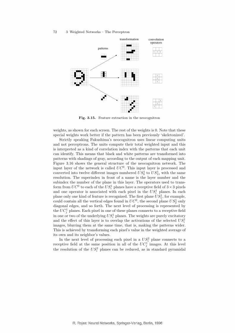
Figure 3.15 shows the general strategy adopted in the neocognitron. Theprojection screen is transformed, deciding for each pixel if it should be keptwhite or black. This can be done by identifying the patterns shown for eachof the three transformations by looking at each pixel and its eight neighbors.In the case of the first transformed screen only horizontal lines are kept;in the second screen only vertical lines and in the third screen only diagonallines. The convolution operators needed have the same distribution of positive




patterns

transformation

1 11

1

1

1

1

1

1

convolutionoperators

Fig. 3.15. Feature extraction in the neocognitron

weights, as shown for each screen. The rest of the weights is 0. Note that thesespecial weights work better if the pattern has been previously ‘skeletonized’.

Strictly speaking Fukushima’s neocognitron uses linear computing unitsand not perceptrons. The units compute their total weighted input and thisis interpreted as a kind of correlation index with the patterns that each unitcan identify. This means that black and white patterns are transformed intopatterns with shadings of gray, according to the output of each mapping unit.Figure 3.16 shows the general structure of the neocognitron network. Theinput layer of the network is called UC0. This input layer is processed andconverted into twelve different images numbered US1

0 to US111 with the same

resolution. The superindex in front of a name is the layer number and thesubindex the number of the plane in this layer. The operators used to trans-form from UC0 to each of the US1

i planes have a receptive field of 3×3 pixelsand one operator is associated with each pixel in the US1

i planes. In eachplane only one kind of feature is recognized. The first plane US1

1 , for example,could contain all the vertical edges found in UC0, the second plane US1

2 onlydiagonal edges, and so forth. The next level of processing is represented bythe UC1

j planes. Each pixel in one of these planes connects to a receptive field

in one or two of the underlying US1i planes. The weights are purely excitatory

and the effect of this layer is to overlap the activations of the selected US1i

images, blurring them at the same time, that is, making the patterns wider.This is achieved by transforming each pixel’s value in the weighted average ofits own and its neighbor’s values.

In the next level of processing each pixel in a US2i plane connects to a

receptive field at the same position in all of the UC1j images. At this level

the resolution of the US2i planes can be reduced, as in standard pyramidal




UC

US planes

UC planes

.

.

. ...

1

1

0

i

j

Fig. 3.16. The architecture of the neocognitron

architectures. Fig 3.16 shows the sizes of the planes used by Fukushima forhandwritten digit recognition. Several layers of alternating US and UC planesare arranged in this way until at the plane UC4 a classification of the hand-written digit in one of the classes 0, . . . , 9 is made. Finding the appropriateweights for the classification task is something we discuss in the next chap-ter. Fukushima has proposed several improvements of the original model [147]over the years.

The main advantage of the neocognitron as a pattern recognition deviceshould be its tolerance to shifts and distortions. Since the UC layers blurthe image and the US layers look for specific features, a certain amount ofdisplacement or rotation of lines should be tolerated. This can happen, but thesystem is highly sensitive to the training method used and does not outperformother simpler neural networks [280]. Other authors have examined variationsof the neocognitron which are more similar to pyramidal networks [463]. Theneocognitron is just an example of a class of network which relies extensivelyon convolution operators and pattern recognition in small receptive fields. Foran extensive discussion of the neocognitron consult [133].




3.4.4 The silicon retina

Carver Mead’s group at Caltech has been active for several years in the fieldof neuromorphic engineering, that is, the production of chips capable of em-ulating the sensory response of some human organs. Their silicon retina, inparticular, is able to simulate some of the features of the human retina.

Mead and his collaborators modeled the first three layers of the retina:the photoreceptors, the horizontal, and the bipolar cells [303, 283]. The hor-izontal cells are simulated in the silicon retina as a grid of resistors. Eachphotoreceptor (the dark points in Figure 3.17) is connected to each of its sixneighbors and produces a potential difference proportional to the logarithmof the luminosity measured. The grid of resistors reaches electric equilibriumwhen an average potential difference has settled in. The individual neurons ofthe silicon retina fire only when the difference between the average and theirown potential reaches a certain threshold.

Fig. 3.17. Diagram of a portion of the silicon retina

The average potential S of n potentials Si can be computed by letting eachpotential Si be proportional to the logarithm of the measured light intensityHi, that is,

S =1

n

n∑

i=1

Si =1

n

n∑

i=1

logHi.

This expression can be transformed into

S =1

nlog(H1H2 · · ·Hn) = log(H1H2 · · ·Hn)1/n.

The equation tells us that the average potential is the logarithm of the ge-ometric mean of the light intensities. A unit only fires when the measuredintensity Si minus the average intensity lies above a certain threshold γ, thatis,

log(Hi)− log(H1H2 · · ·Hn)1/n ≥ γ,



3.5 Historical and bibliographical remarks 75

and this is valid only when

logHi

(H1H2 · · ·Hn)1/n≥ γ.

The units in the silicon retina fire when the relative luminosity of a pointwith respect to the background is significantly higher, such as in a humanretina. We know from optical measurements that when outside on a sunnyday, the black letters in a book reflect more photons on our eyes than whitepaper does in a room. Our eyes adjust automatically to compensate for theluminosity of the background so that we can recognize patterns and readbooks inside and outside.

3.5 Historical and bibliographical remarks

The perceptron was the first neural network to be produced commercially,although the first prototypes were used mainly in research laboratories. FrankRosenblatt used the perceptron to solve some image recognition problems[185]. Some researchers consider the perceptron as the first serious abstractmodel of nervous cells [60].

It was not a coincidence that Rosenblatt conceived his model at the end ofthe 1950s. It was precisely in this period that researchers like Hubel and Wieselwere able to “decode” the structure of the retina and examine the structureof the receptive fields of neurons. At the beginning of the 1970s, researchershad a fair global picture of the architecture of the human eye [205]. DavidMarr’s influential book Vision offered the first integrated picture of the visualsystem in a way that fused biology and engineering, by looking at the way thevisual pathway actually computed partial results to be integrated in the rawvisual sketch.

The book Perceptrons by Minsky and Papert was very influential amongthe AI community and is said to have affected the strategic funding decisionsof research agencies. This book is one of the best ever written on its subjectand set higher standards for neural network research, although it has beencriticized for stressing the incomputability, not the computability results. TheDreyfus brothers [114] consider the reaction to Perceptrons as one of the mile-stones in the permanent conflict between the symbolic and the connectionistschools of thought in AI. According to them, reaction to the book opened theway for a long period of dominance of the symbolic approach. Minsky, for hispart, now propagates an alternative massively parallel paradigm of a societyof agents of consciousness which he calls a society of mind [313].

Convolution operators for image processing have been used for many yearsand are standard methods in the fields of image processing and computervision. Chips integrating this kind of processing, like the silicon retina, havebeen produced in several variants and will be used in future robots. Someresearchers dream of using similar chips to restore limited vision to blind




persons with intact visual nerves, although this is, of course, still an extremelyambitious objective [123].

Exercises

1. Write a computer program that counts the number of linearly separableBoolean functions of 2, 3, and 4 arguments. Hint: Generate the perceptronweights randomly.

2. Consider a simple perceptron with n bipolar inputs and threshold θ = 0.Restrict each of the weights to have the value −1 or 1. Give the smallestupper bound you can find for the number of functions from {−1, 1}n to{−1, 1} which are computable by this perceptron [219]. Prove that theupper bound is sharp, i.e., that all functions are different.

3. Show that two finite linearly separable sets A and B can be separated bya perceptron with rational weights. Note that in Def. 2 the weights arereal numbers.

4. Prove that the parity function of n > 2 binary inputs x1, x2, . . . , xn cannotbe computed by a perceptron.

5. Implement edge detection with a computer program capable of processinga computer image.

6. Write a computer program capable of simulating the silicon retina. Showthe output produced by different pictures on the computer’s screen.


3 Weighted Networks – The Perceptron - Freie Universität · 2008-01-11 · 3 Weighted Networks...

Documents

Transcript of 3 Weighted Networks – The Perceptron - Freie Universität · 2008-01-11 · 3 Weighted Networks...