3 Phase Plane

8/4/2019 3 Phase Plane

http://slidepdf.com/reader/full/3-phase-plane 1/23

3 Phase-Plane Analysis

Phase plane analysis is a technique for the analysis of the qualitative behavior of second-

order systems. It provides physical insights.

Reference: Graham and McRuer, Analysis of Nonlinear Control Systems, Dover Press,

1971.

Consider the second-order system described by the following equations:

),( 211 x x p x =&

),( 212 x xq x =&

x1 and x2 are states of the system

p and q are nonlinear functions of the states

Key points

• Phase plane analysis is limited to second-order systems.

• For second order systems, solution trajectories can be represented by curves inthe plane, which allows for visualization of the qualitative behavior of the

system.

• In particular, it is interesting to consider the behavior of systems around

equilibrium points.



phase plane = plane having x1 and x2 as coordinates

→ get “rid” of time

),(

),(

21

21

1

2

x x p

x xq

dx

dx =

We look for equilibrium points of the system (also called singular points), i.e. points atwhich:

0),( 21 =ee x x p

0),( 21 =ee x xq

Example:

Find the equilibrium point(s) of the system described by the following equation:

32)( xa x x &&& +−=

Start by putting the system in the standard form by setting 21 , x x x x == & :

3

2

2

12

21

)( xa x x

x x

+−=

=

&

&

Looking at the slope of the phase plane trajectory:

2

3

2

2

1

1

2 )(

x

xa x

dx

dx +−=

This yields the following equilibrium point:

02

1

=

=

e

e

x

a x

Investigate the linear behaviour about a singular point:

111 x x x e δ +=

222 x x x e δ +=



22

11

1 x x

p x

x

p x

ee

δ δ δ ∂∂

+∂∂

=&

22

11

2 x x

q x

x

q x

ee

δ δ δ ∂∂

+∂∂

=&

Seteeee

x

qd

x

qc

x

pb

x

pa

2121,,,

∂∂

=∂∂

=∂∂

=∂∂

=

Then

211 xb xa x δ δ δ +=&

212 xd xc x δ δ δ +=&

This is the general form of a second-order linear system.

Next, we obtain the characteristic equation:

0))(( =−−− bcd a λ λ

This equation admits the roots:

2

)(4)( 22,1

bcad ad d a

−−±+=λ

This yields the following possible cases:

λ1, λ2 real and negative Stable node

λ1, λ2 real and positive Unstable node

λ1, λ2 real and opposite signs Saddle point

λ1, λ2 complex and negative real parts Stable focus

λ1, λ2 complex and positive real parts Unstable focus

λ1, λ2 complex and zero real parts Center



Stability (Lyapunov’s First Method)

Consider the system described by the equation:

)( x f x =&

Write x as : x x x e δ +=

Then ),(.),(. x xh x A x x xh x x

f x ee

e

δ δ δ δ δ δ +=⇒+∂

∂= &&

Lyapunov proved that the eigenvalues of A indicate “local” stability of the nonlinear system about the equilibrium point if:

a) 0),(

lim0

=→ x

x xh e

x δ

δ

δ

(“The linear terms dominate”)

b) There are no eigenvalues with zero real part.

Example:

Consider the equation:

3 xax x +−=&

If x is small enough, then 3 xax >>

Thought question: What if a = 0?



Example: Simplified satellite control problem

Built in the 1960s.

After about one month, would run out of gas.

How was the controller designed?

),( θ θ θ &&& T T =

Let’s pick 0=desθ .

θ θ θ &&&21 ccT −−=

It’ cold in space: the valves would freeze open. If θ and θ & are small, there is not enough

torque to break the ice, so the valves get frozen open and all the gas escapes. One

solution is either relay control and / or bang-bang control. (These methods are inelegant).

Pick I T u /= , and u=θ && .

θ θ

θ

&

& u

d

d =

Case 1: Pick u = 0. The satellite just floats.



In the “thick black line” interval, all trajectories point towards the switching line.



Bad idea!

On the line, 0=+ θ θ a& . (a>0).

On average: at

AVG AVG AVG et a −=⇒=+ 0)(0 θ θ θ θ &

On the average, the trajectory goes to the origin.

Introduction to Sliding Mode Control (also called Variable Structure Control)

Consider the system governed by the equation:

u=θ &&

Inspired by the previous example, we select a control law of the form:

)sgn( sU u m−=

where ),( θ θ & s s = . How should we pick the function s?



Case 1: θ = s

This does not yield the performance we want.

Case 2: θ &= s

This does not yield the performance we want.

Case 3: θ θ a s += &

)sgn()sgn( θ θ θ θ aU sU u mm +−=⇒−== &&&&&

θ θ θ θ &&&&& a sa s +=⇒+=



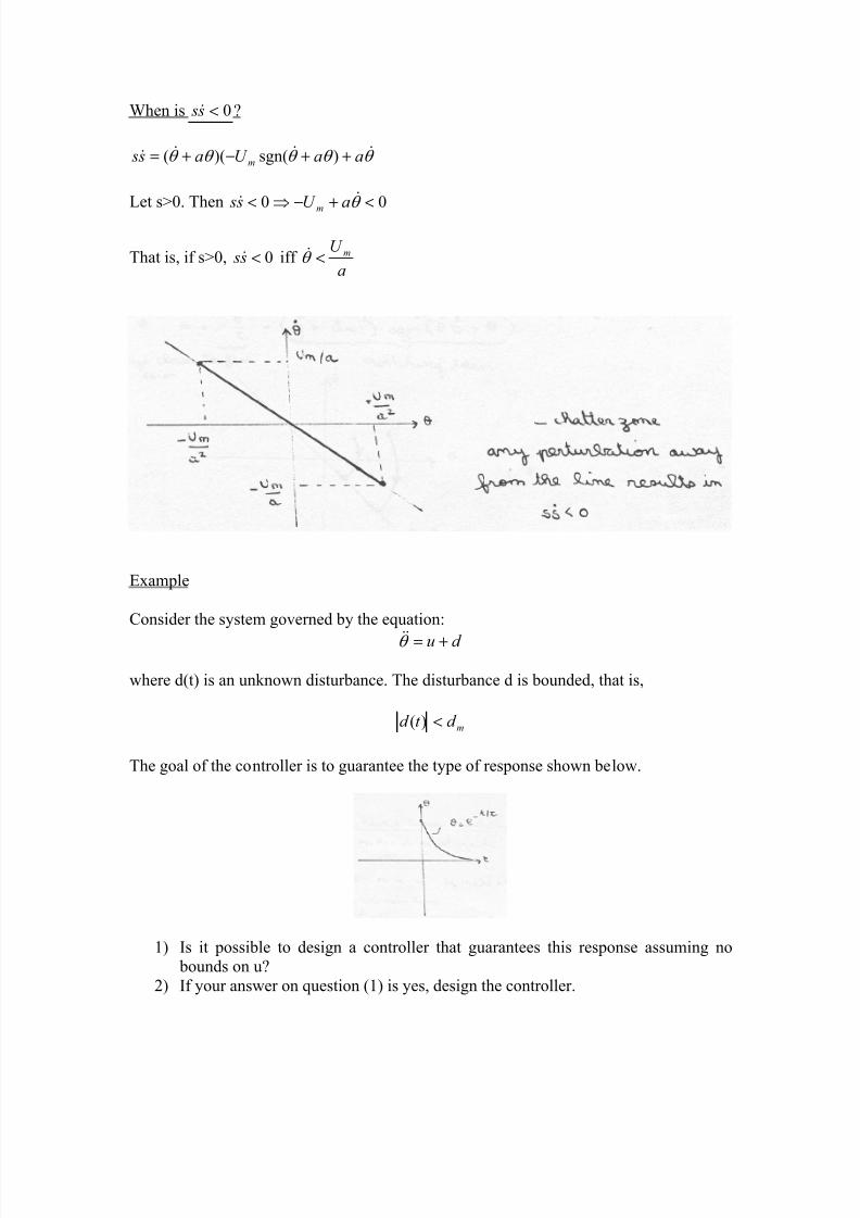
When is 0< s s& ?

θ θ θ θ θ &&&& aaU a s s m++−+= )sgn()((

Let s>0. Then 00 <+−⇒< θ && aU s sm

That is, if s>0, 0< s s& iff a

U m<θ &

Example


d u +=θ &&

where d(t) is an unknown disturbance. The disturbance d is bounded, that is,

md t d <)(

The goal of the controller is to guarantee the type of response shown below.

1) Is it possible to design a controller that guarantees this response assuming no bounds on u?

2) If your answer on question (1) is yes, design the controller.



The desired behavior is a first-order response. Define θ θ τ += & s

If s=0, we have the desired system response. Hence our goal is to drive s to zero.

If u appears in the equation for s, set s=0 and solve for u. Unfortunately, this is not the

case. Keep differentiating the equation for s until u appears.

θ τ τ θ τ θ θ τ &&&&&& ++=++=+= )())(( t d ut d u s

Look for the condition for 0< s s& .

0))()((0 <+++⇒< θ τ τ θ θ τ &&& t d u s s

We therefore select u to be:

)sgn()( θ θ τ η τ θ ++−−= &

&

md u

The first term dictates that one always approaches zero. The second term is called the

switching term. The parameter η is a tuning parameter that governs how fast one goes tozero.

Once the trajectory crosses the s=0 line, the goals are met, and the system “slides”

along the line. Hence the name sliding mode control.

Does the switching surface s have to be a line?

No, but it keeps the problem analyzable.

Example of a nonlinear switching surface




u x =&&

For a mechanical system, an analogy would be making a cart reach a given position atzero velocity in minimal time.

The request for a minimal time solution suggests a bang-bang type of approach.

This can be obtained, for example, with the following expression for s:

02

1),( =+= xU x x x x s m

&&&

The shape of the sliding surface is as shown below.

This corresponds to the following block diagram:

Logic is missing for the case when s is exactly equal to zero. In practice for a

continuous system such as that shown above this case is never reached.



Classical Phase-Plane Analysis Examples

Reference: GM Chapter 7

Example: Position control servo (rotational)

Case 1: Effect of dry friction

The governing equation is as follows:

000 )sgn( θ θ θ K B I −−= &&&

For simplicity and without lack of generality, assume that I = 1. Then:

)sgn(1

000 θ θ θ &&&

K

B

K

−=+

That yields:

0

00

0

0

)sgn(

θ

θ θ

θ

θ

&

&&

−−

=K

B K

d

d



The friction function is given by:

There are an infinite number of singular points, as shown below:

When 00 >θ & , we have K

B

K −=+ 00

1θ θ && , that is, we have an undamped linear oscillation

( a center). Similarly, when 00 <θ & , we have K

B

K +=+ 00

1θ θ && (another center).

From a controls perspective, dry friction results in an offset, that is, a loss of static

accuracy.

To get the accuracy back, it is possible to introduce dither into the system. Dither is ahigh-frequency, low-amplitude disturbance (an analogy would be tapping an offset scale

with one’s finger to make it return to the correct value).



The effects of saturation do not look destabilizing. However, saturation affects the

performance by “slowing it down”.

The effect of saturation is to “slow down” the system.

Note that we are assuming here that the system was stable to start with before we applied

saturation.

Problems appear if one is not operating in the linear region, which indicates that the gain

should be reduced in the saturated region.

If you increase the gain of a linear system oftentimes it eventually winds up unstable,except if the root locus looks like:

Root locus for a conditionally stable system (for example an inverted pendulum).

So there are systems for which saturation will make you unstable.



SUMMARY: Second-Order Systems and Phase-Plane Analysis

• Graphical Study of Second-Order Autonomous Systems

),( 211 x x p x =&

),( 212 x xq x =&

x1 and x2 are states of the system

p and q are nonlinear functions of the states

phase plane = plane having x1 and x2 as coordinates

→ get “rid” of time

As t goes from 0 → +∞, and given some initial conditions, the solution x(t) can berepresented geometrically as a curve (a trajectory) in the phase plane. The family of

phase-plane trajectories corresponding to all possible initial conditions is called the phase

portrait .

• Due to Henri Poincaré

French mathematician, (1854-1912).

Main contributions:

Algebraic topology Differential Equations Theory of complex variables

Orbits and Gravitation http://www-history.mcs.st-andrews.ac.uk/history/Mathematicians/Poincare.html

Poincaré conjecture

In 1904 Poincaré conjectured that any closed 3-dimensional manifold which is homotopy

equivalent to the 3-sphere must be the 3-sphere. Although higher-dimensional analoguesof this conjecture have been proved, the original conjecture remains open.

• Equilibrium (singular point)

Singular point = equilibrium point in the phase plane

0),( 21 =ee x x p



0),( 21 =ee x xq

Slope of the phase trajectory

),(

),(

21

21

1

2

x x p

x xq

dx

dx =

At an equilibrium point, the value of the slope is indeterminate (0/0) → “singular” point.

• Investigate the linear behaviour about a singular point

111 x x x e δ +=

222 x x x e δ +=

22

11

1 x x

p x

x

p x

ee

δ δ δ ∂∂

+∂∂

=&

22

11

2 x x

q x

x

q x

ee

δ δ δ ∂∂

+∂∂

=&

Seteeee

x

qd

x

qc

x

pb

x

pa

2121,,,

∂∂

=∂∂

=∂∂

=∂∂

=

Then

211 xb xa x δ δ δ +=&

212 xd xc x δ δ δ +=&

Which is the general form of a second-order linear system.

• Obtain the characteristic equation

0))(( =−−− bcd a λ λ

This equation admits the roots:

2

)(4)( 22,1

bcad ad d a

−−±+=λ

• Possible cases

Pictures are from H. Khalil, Nonlinear Systems, Second Edition.



λ 1 and λ 2 are real and negative

STABLE NODE

σ

jω

λ 1 and λ 2 are real and positive

UNSTABLE NODE

σ

jω

λ 1 and λ 2 are real and of opposite sign

SADDLE POINT (UNSTABLE)

σ

jω

λ 1 and λ 2 are complex with negative real

parts

STABLE FOCUS

σ

jω



λ 1 and λ 2 are complex with positive real parts

UNSTABLE FOCUS

σ

jω

λ 1 and λ 2 are complex with zero real parts

CENTER

σ

jω

• Which direction do circles and spirals spin, and what does this mean?

Consider the system:

21

21

x x x x σ ω ω σ −=&&

Let 22

21 x xr += and

1

2arctan x x=φ .

With ½ page of straightforward algebra, one can show that: (see homework 1 for details)

r r σ =& and ω φ −=&

The “r” equation says that in a Jordan block, the diagonal element, σ, determines whether

the equilibrium is stable. Since r is always non-negative, σ greater than zero gives agrowing radius (unstable), while σ less than zero gives a shrinking radius. ω gives the rateand direction of rotation, but has no effect on stability. For a given physical system,

simply re-assigning the states can get either positive or negative ω.

In summary:



If σ > 0, the phase plot spirals outwards.

If σ < 0, the phase plot spirals inwards.

If ω > 0, the arrows on the phase plot are clockwise.

If ω < 0, the arrows on the phase plot are counter-clockwise.

• Stability

)( x f x=&

x=xe+δx

e x x

f A

=∂∂

=

),( x xeh x A x δ δ δ +=&

Lyapunov proved that the eigenvalues of A indicate “local” stability if:

(a) “the linear terms dominate”, that is:

0),(

lim0

=→ x

x xeh

x δ

δ

δ

(b) there are no eigenvalues with zero real part.



Practice Problems

Second Order Systems and Phase Plane Analysis

Exercise 1

For each system, construct the phase portrait (preferably without using a computer

program). Discuss the qualitative behavior of the system.

(a)

=

=

12

121

sin

cos

x x

x x x

&

&

(b)

−++=

−+−=

)1)((

)1)((2

2

2

1212

2

2

2

1211

x x x x x

x x x x x

&

&

Exercise 2

For each system, find all equilibrium points and determine the type of each isolated

equilibrium.

(a)

−−=

++=

21212

2

1211

234

43

x x x x x

x x x x

&

&

(b)

−=

−+= −

122

21

sin

1 1

x x x

e x x x

&

&

(c)

+−=

+=

212

2

121

42

2

x x x

x x x

&

&

3 Phase Plane

Documents

Transcript of 3 Phase Plane