Digital Image Compression Using Wavelets

Kristy VanHornweder

July 2004

Department of Mathematics and Statistics

University of Minnesota Duluth

UNIVERSITY OF MINNESOTA

This is to certify that I have examined this copy of a master’s project by

Kristy Sue VanHornweder

and have found that it is complete and satisfactory in all respects, and that any and all revisions required by the final examining committee have

been made.

Robert L. McFarland____________________________________________

Name of Faculty Advisor

____________________________________________Signature of Faculty Advisor

____________________________________________Date

Digital Image Compression Using Wavelets

A PROJECT SUBMITTED TO THE FACULTY OF THE GRADUATE SCHOOL OF THE UNIVERSITY OF MINNESOTA

BY

Kristy Sue VanHornweder

IN PARTIAL FULFILLMENT OF THE REQUIREMENTS FOR THE DEGREE OF MASTER OF SCIENCE

Department of Mathematics and Statistics

University of Minnesota Duluth

July 2004

Kristy Sue VanHornweder 2004

Acknowledgements

There are several people I would like to acknowledge for contributing to the devel-opment of this paper.

First, I would like to thank my advisor Dr. Robert L. McFarland for all the assistance he has given me in understanding the mathematical details and for providing the idea for a project on an interesting topic.

I would like to thank Dr. Bruce Peckham and Dr. Doug Dunham for reading a prelim-inary version of this paper and making suggestions for improvement.

Lastly, I would like to thank the UMD Mathematics and Statistics Department for providing me the opportunity of pursuing a graduate degree in Applied and Computa-tional Mathematics and undertaking a masters project in an interesting area.

i.

Contents

1. Introduction and Motivation.................................................................................1

2. Previous Image Compression Techniques...........................................................4

3. Filters and Filter Banks.........................................................................................7 3.1. Averages and Differences.........................................................................7 3.2. Convolution...............................................................................................93.3. Low-pass Filter.......................................................................................11 3.4. High-pass Filter.......................................................................................133.5. Low-pass Filter and High-pass Filter in the Frequency Domain.............143.6. Analysis and Synthesis Filter Banks........................................................203.7. Iterative Filtering Process........................................................................293.8. Fast Wavelet Transform..........................................................................33

4. Wavelet Transformation......................................................................................374.1. Introduction to Haar Wavelets.................................................................374.2. Scaling Function and Equations..............................................................374.3. Wavelet Function and Equations.............................................................404.4. Orthonormal Functions............................................................................434.5. The Theory Behind Wavelets..................................................................474.6. The Connection Between Wavelets and Filters.......................................554.7. Daubechies Wavelets...............................................................................574.8. Two Dimensional Wavelets.....................................................................66

5. Image Compression Using Wavelets...................................................................695.1. Wavelet Transform of Images.................................................................695.2. Zero-Tree Structure.................................................................................805.3. Idea of the Image Compression Algorithm.............................................845.4. Bit Plane Coding......................................................................................875.5. EZW Algorithm.......................................................................................875.6. EZW Example.........................................................................................885.7. Decoding the Image...............................................................................1055.8. Inverse Wavelet Transform...................................................................1085.9. Extension of EZW.................................................................................1125.10. Demonstration Software......................................................................113

6. Performance of Wavelet Image Compression..................................................114

ii.7. Applications of Wavelet Image Compression..................................................118

7.1. Medical Imaging....................................................................................1187.2. FBI Fingerprinting.................................................................................1197.3. Computer 3D Graphics..........................................................................1207.4. Space Applications................................................................................1227.5. Geophysics and Seismics.......................................................................1237.6. Meteorology and Weather Imaging.......................................................1247.7. Digital Photography...............................................................................1257.8. Internet/E-commerce.............................................................................126

Appendix: Proofs of Theorems..............................................................................127

References................................................................................................................130

iii.

List of Figures

Figure 1.a. No changes.................................................................................................2Figure 1.b. Many changes.............................................................................................2Figure 2. DCT encoding process..................................................................................4Figure 3. DCT decoding process..................................................................................4Figure 4a. Original image.............................................................................................5Figure 4b. Reconstructed image using DCT.................................................................5Figure 5. Tree structure of averages and differences (4 input elements)......................9Figure 6. Plot of magnitude of H0(ω)........................................................................18Figure 7. Plot of magnitude of H1(ω)........................................................................19Figure 8. Analysis Filter Bank....................................................................................22Figure 9. Synthesis Filter Bank..................................................................................26Figure 10. Entire Filter Bank.....................................................................................28Figure 11. Two pass analysis bank.............................................................................30Figure 12. Three pass analysis bank...........................................................................31Figure 13. Tree structure for filter bank with 8 input elements..................................32Figure 14. Scaling function φ(t)..................................................................................38Figure 15. Scaling function φ(2t)................................................................................38Figure 16. Scaling function φ(2t–1)............................................................................38Figure 17. Scaling function φ(4t)................................................................................39Figure 18. Scaling function φ(4t–1)............................................................................39Figure 19. Scaling function φ(4t –2)...........................................................................39Figure 20. Scaling function φ(4t–3)............................................................................39Figure 21. Wavelet function w(t)................................................................................41Figure 22. Wavelet function w(2t)..............................................................................42

Figure 23. Wavelet function w(2t–1)..........................................................................42Figure 24. Wavelet function w(4t)..............................................................................42Figure 25. Wavelet function w(4t–1)..........................................................................42Figure 26. Wavelet function w(4t–2)..........................................................................43Figure 27. Wavelet function w(4t–3)..........................................................................43Figure 28. Scaling function φ0,0(t)...............................................................................52Figure 29. Wavelet function w0,0(t).............................................................................52Figure 30. Scaling function φ1,0(t)...............................................................................52Figure 31. Scaling function φ1,1(t)...............................................................................52Figure 32. Derivation of basis for U j.........................................................................54Figure 33. D4 wavelet.................................................................................................63Figure 34. D6 wavelet.................................................................................................63Figure 35. Daubechies graphs showing improvement in flatness..............................65Figure 36. 2D wavelet w(2s) w(2t).........................................................................67Figure 37. 2D wavelet w(2s) w(2t–1).....................................................................67

iv.Figure 38. 2D wavelet w(2s–1) w(2t).....................................................................68Figure 39. 2D wavelet w(2s–1) w(2t–1).................................................................68Figure 40. One level decomposition...........................................................................69Figure 41. House example..........................................................................................70Figure 42. One level decomposition of house example..............................................70Figure 43. Three level decomposition........................................................................72Figure 44. Three level decomposition of house example...........................................72Figure 45. Filter diagram for three iterations of two-dimensional wavelet................73Figure 46. Example image used for calculating decomposition.................................74Figure 47. Wavelet transform of pixel array representing the image in Figure 46... .80Figure 48. Zero-tree structure.....................................................................................82Figure 49. Zero-tree structure for HH3 band in Figure 47..........................................83Figure 50. Scan order used in the EZW algorithm.....................................................85Figure 51. Reconstruction after one iteration of EZW...............................................92Figure 52. Reconstruction after two iterations of EZW.............................................95Figure 53. Reconstruction after three iterations of EZW...........................................97Figure 54. Reconstruction after four iterations of EZW...........................................100Figure 55. Reconstruction after five iterations of EZW...........................................101Figure 56. Reconstruction after six iterations of EZW.............................................103Figure 57. Progressive refinement of image given in Figure 46..............................104Figure 58. Partial output file for EZW example.......................................................105Figure 59. Symbol array of third iteration of decoding process...............................107Figure 60. Reconstruction of wavelet coefficients in decoding process..................108Figure 61. Comparison of compression algorithms..................................................114Figure 62. Barbara image using JPEG (left) and EZW (right) ................................115Figure 63. Lena reconstructed using 10% and 5% of the coefficients using D4

wavelets...................................................................................................115

Figure 64. Winter original and reconstruction using 10% of the coefficients using D4 wavelets...................................................................................................116Figure 65. Graph of results of Lena and Winter images for three wavelet methods117Figure 66. Medical image reconstructed from lossless and 20:1 lossy compression118Figure 67. Progressive refinement of medical image...............................................119Figure 68. FBI fingerprint image showing fine details.............................................120Figure 69. Progressive refinement (from right to left) of 3D model........................121Figure 70. FlexWave II architecture.........................................................................122Figure 71. Reconstructions of aerial image using CCSDS, JPEG, and JPEG2000..123Figure 72. Brain image, original on left, reconstruction on right.............................124

v.

List of Tables

Table 1. Multimedia data along with uncompressed size and transmission time.........1Table 2. Coefficients for D4........................................................................................64Table 3. Coefficients for D6....................................................................................... 64Table 4. Indexing scheme for coefficients..................................................................83Table 5. First dominant pass of EZW example..........................................................90Table 6. Second dominant pass of EZW example......................................................92Table 7. Second subordinate pass of EZW example..................................................93Table 8. Third dominant pass of EZW example.........................................................95Table 9. Intervals for third subordinate pass of EZW example..................................96Table 10. Third subordinate pass of EZW example...................................................96Table 11. Partial fourth dominant pass of EZW example..........................................98Table 12. Fourth subordinate pass of EZW example.................................................99Table 13. Partial fifth subordinate pass of EZW example........................................100Table 14. Partial sixth subordinate pass of EZW example.......................................102Table 15. Partial seventh subordinate pass of EZW example..................................103Table 16. Results of three wavelet methods on Lena image....................................116Table 17. Results of three wavelet methods on Winter image.................................117

vi.

List of Key Equations

(1) Discrete Cosine Transform (DCT)..........................................................................5(2) Convolution...........................................................................................................10(3) Low-pass filter......................................................................................................11(4) High-pass filter......................................................................................................13(5) DeMoivre’s Theorem............................................................................................15(6) Low-pass response in frequency domain..............................................................17(7) High-pass response in frequency domain.............................................................19(8) Low-pass output of analysis bank.........................................................................22(9) High-pass output of analysis bank........................................................................22(10) Number of multiplications in Fast Wavelet Transform......................................35(11) Scaling (box) function.........................................................................................37(12) Basic dilation equation........................................................................................39(13) General dilation equation....................................................................................40(14) Basic wavelet equation........................................................................................40(15) General wavelet equation....................................................................................41(16) Inner product.......................................................................................................43(17) Condition for orthogonality................................................................................44(18) Condition for orthonormality..............................................................................44(19) Support of scaling functions...............................................................................48(20) Normalized general dilation equation.................................................................50(21) Normalized general wavelet equation.................................................................51(22) Condition on coefficients for D4 wavelets..........................................................60(23) Condition on coefficients for D4 wavelets..........................................................60(24) Condition on coefficients for D4 wavelets..........................................................60

(25) Condition on coefficients for D4 wavelets..........................................................61(26) Condition on coefficients for D6 wavelets..........................................................63(27) Condition on coefficients for D6 wavelets..........................................................63(28) Wavelet transform on row of image...................................................................66(29) Wavelet transform on column of image..............................................................67(30) Initial threshold for EZW algorithm...................................................................85

vii.

Abstract

Digital images are being used in an ever increasing variety of applications; examples include medical imaging, FBI fingerprinting, space applications, and e-commerce. As more and more digital images are used, it is necessary to implement effective image compression schemes for reducing the storage space needed to archive images and for minimizing the transmission time for sending images over networks with limited bandwidth.

This paper will discuss and demonstrate the EZW (Embedded Zero-tree Wavelet) image compression algorithm, which is used in the JPEG2000 image processing stan-dard. This algorithm permits the progressive transmission of an image by building a multi-layered framework of the image at varying levels of resolution, ranging from the coarsest approximation to finer and finer details at each iteration. This paper will also develop the necessary background material for understanding the image comp-ression algorithm. The concept of filtering will be discussed, in which an image is separated into low-frequency and high-frequency components at varying levels of de-tail. Wavelet functions will also be discussed, beginning with the basic Haar wavelet and progressing to the more complex Daubechies wavelets. Information and tech-niques of several real-world applications of image compression techniques using wav-elets will also be presented.

There are numerous sources that present and discuss wavelets and image compression, at varying levels of difficulty. This work is intended to serve as a tutorial for indivi-duals who are unfamiliar with these concepts. It should be readable by graduate stu-dents and advanced undergraduate students in Mathematics,

Computer Science, and Electrical Engineering. A background of elementary linear algebra is assumed.

viii.

1. Introduction and Motivation

As digital images become more widely used, it becomes more important to develop

effective image compression techniques. The two main concerns when dealing with

images are storage space and transmission time. Table 1 gives storage size and trans-

Table 1. Multimedia data along with uncompressed size and transmission time (Extracted from [13])

mission times for four different types of data. It is clear, especially in the case of

video, that these figures are unacceptable for practical applications. Therefore, there

is a need to find a way of compressing the image. Image compression techniques re-

duce the number of bits that are needed to represent an image, and this reduces the

needed storage space and transmission time considerably.

The things to look for in compressing an image are redundancy and patterns. Redun-

dancy is reduced or eliminated by removing duplication that occurs in the image.

There is often correlation between neighboring pixels in an image, which is referred

to as spatial redundancy. In the natural world, there are numerous occurrences of re-

dundancy and patterns. For example, in an outdoor image, portions of the sky may

have a uniform consistency. It is not necessary to store every pixel since there is very

little change from one pixel to the next. As another example, consider a brick pattern

of a building. This pattern repeats itself over and over, and so only one instance of

the pattern needs to be retained and the rest of the occurrences are simply a copy, ex-

cept for their location in the image. Another type of reduction is that of irrelevancy,

1

where subtle portions that go unnoticed are removed from the image.

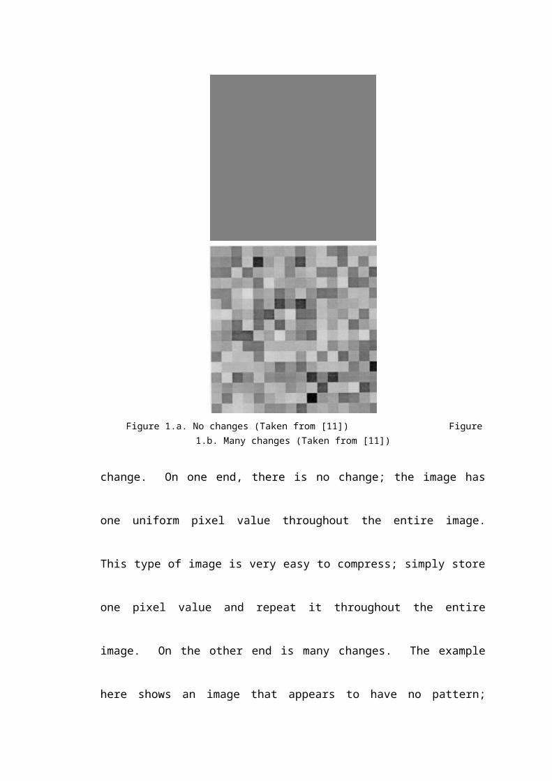
When looking for patterns in an image, one technique is to consider how much

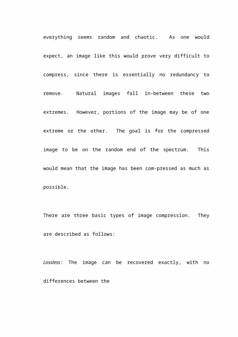
change there is throughout the image. Figure 1 shows the two extremes in amount of

Figure 1.a. No changes (Taken from [11]) Figure 1.b. Many changes (Taken from [11])

change. On one end, there is no change; the image has one uniform pixel value

throughout the entire image. This type of image is very easy to compress; simply

store one pixel value and repeat it throughout the entire image. On the other end is

many changes. The example here shows an image that appears to have no pattern;

everything seems random and chaotic. As one would expect, an image like this would

prove very difficult to compress, since there is essentially no redundancy to remove.

Natural images fall in-between these two extremes. However, portions of the image

may be of one extreme or the other. The goal is for the compressed image to be on

the random end of the spectrum. This would mean that the image has been com-

pressed as much as possible.

There are three basic types of image compression. They are described as follows:

Lossless: The image can be recovered exactly, with no differences between the

2

reconstructed image and the original image. There is no information lost in the com-

pression process. The disadvantage of this type of compression is that not very much

compression can be achieved.

Lossy: There is information of the image that is lost during the compression process,

thus, the reconstructed image will not be identical to the original image. The recon-

structed image will not be of quite as good quality, but much higher compression rates

are possible.

Near lossless: This is in-between the other two types of compression. There is some

information lost, but the lost information is insignificant and likely will not be per-

ceivable. The compression rate is also in-between that of the other two methods.

The description of the above three methods imply that there is a tradeoff between the

amount of compression that can be achieved, and the quality of the reconstructed

image. It is important to find a balance between these two, and to find a combination

that is reasonable.

The purpose of this paper is to serve as a tutorial. There are numerous sources of in-

formation about image compression and wavelets, at varying levels of complexity.

Many of the sources are very complicated and require a significant background in cer-

tain mathematical and/or engineering concepts. This paper will attempt to demon-

strate and explain the basic ideas behind wavelets and image compression so that they

are fairly simple and straightforward to understand. This paper should be readable by

graduate students and advanced undergraduate students in Mathematics, Computer

Science, and Electrical Engineering. Some basic background in mathematics is as-

sumed, primarily, introductory linear algebra.

3

2. Previous Image Compression Techniques

In 1992, the JPEG (Joint Photographic Experts Group) image compression standard

was established by ISO (International Standards Organization) and IEC (International

Electro-Technical Commission) [13]. This method uses the DCT (Discrete Cosine

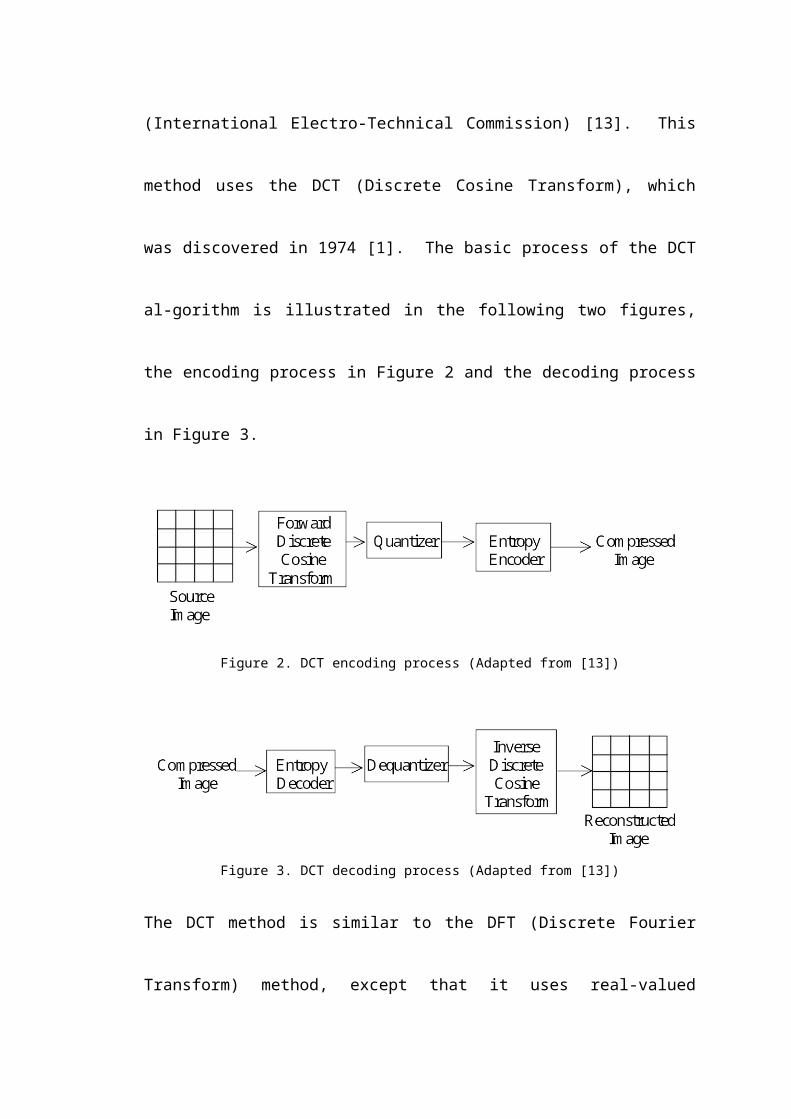
Transform), which was discovered in 1974 [1]. The basic process of the DCT al-

gorithm is illustrated in the following two figures, the encoding process in Figure 2

and the decoding process in Figure 3.

Figure 2. DCT encoding process (Adapted from [13])

Figure 3. DCT decoding process (Adapted from [13])

The DCT method is similar to the DFT (Discrete Fourier Transform) method, except

that it uses real-valued coefficients, and that fewer coefficients are used while a better

approximation is obtained. The algorithm uses O(nlgn) operations, whereas the DFT

method uses O(n2) operations. The formula for the DCT is shown below [13], as-

suming x(n), where n = 0, 1, ..., N 1 is a discrete input signal:

4

(1)

The Forward DCT encoder divides the image into 8×8 blocks and applies the DCT

transformation to each of them. Most of the spatial frequencies have zero or near-

zero amplitude, so they do not need to be encoded. The output from this transforma-

tion is then quantized using a quantization table. The number of bits representing the

image is reduced by reducing the precision of the coefficients representing the image.

The resulting coefficients are then ordered so that low frequency coefficients appear

before high frequency ones. The last step in the compression process is entropy en-

coding, which compresses the image further, and does so losslessly. The image is

compacted further by using statistical properties of the coefficients. A Huffman [22]

or arithmetic [21] encoding algorithm can be used for this process.

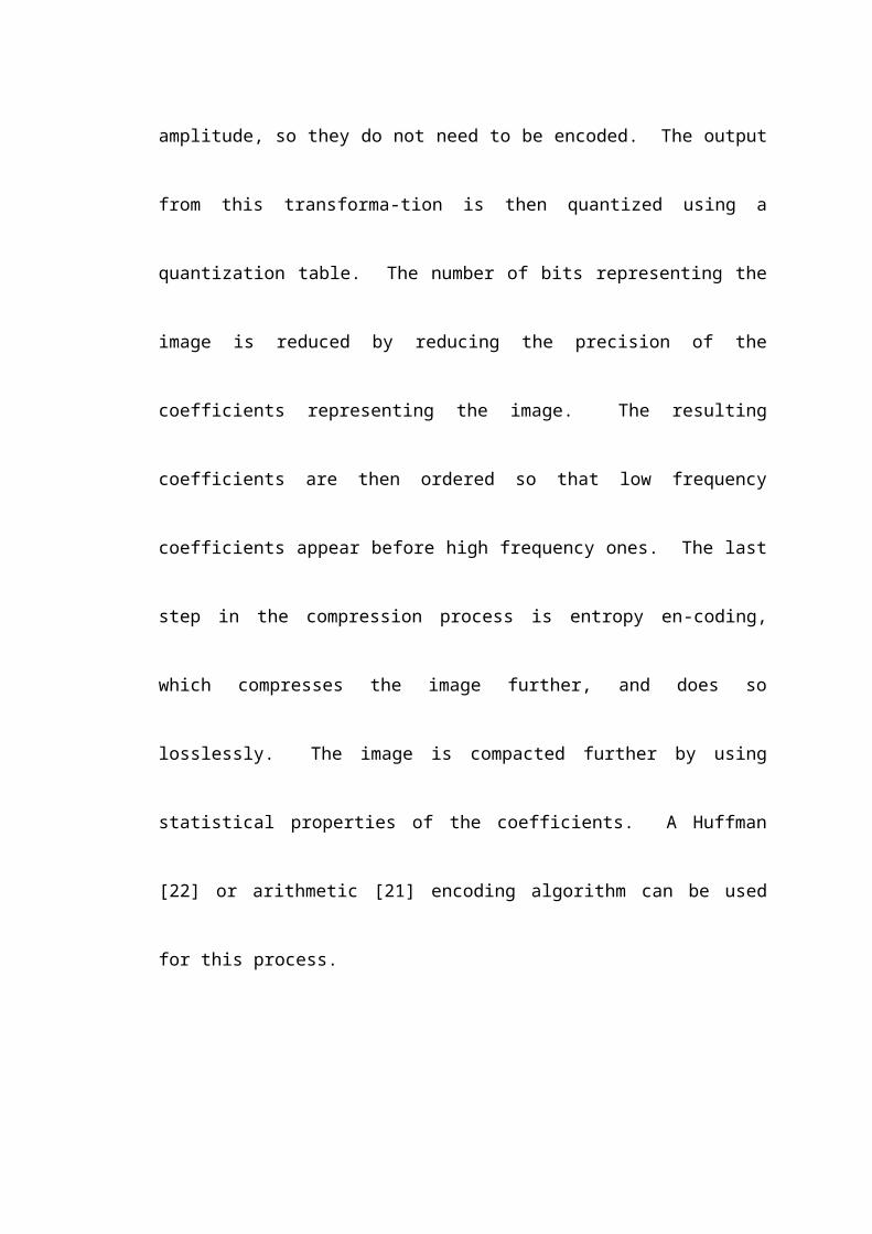
The DCT method is fairly easy to implement, but a major disadvantage is that it re-

sults in blocking artifacts in the reconstructed image. In Figure 4, the second image

clearly shows the introduction of blocking into the image. The reason for this is that

Figure 4a. Original image (Taken from [13]) Figure 4b. Reconstructed image using DCT

(Taken from [13])

5each 8×8 block is treated separately. The algorithm does not consider boundaries bet-

ween blocks, so it does nothing to attempt to piece them together to obtain a smoother

image. This disadvantage is the main reason why techniques using wavelet trans-

forms are preferred. In addition to eliminating blockiness, wavelets are more resistant

to errors introduced by noise, higher compression rates are achievable, the image does

not need to be separated into 8×8 blocks, and wavelet techniques allow for progress-

sive transmission or refinement of the image. The quality of the image improves gra-

dually with each step of the algorithm, as the image is fine-tuned. The process can be

terminated at any stage, depending on the desired compression rate or image quality.

This is related to the idea of multiresolution, where several levels of detail of the

image are represented.

Image compression techniques using wavelets will be discussed in a later section.

Before that, it is necessary to introduce some background concepts, as they will be

needed to understand the image compression process. The major concepts are filters

and filterbanks, and wavelet transformations.

6

3. Filters and Filter Banks

This section will introduce the basic concepts of filters and filter banks that are neces-

sary for understanding image compression.

3.1. Averages and Differences

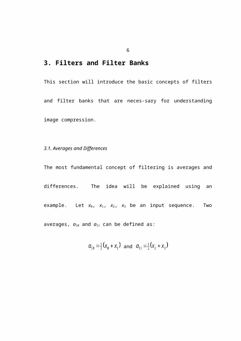
The most fundamental concept of filtering is averages and differences. The idea will

be explained using an example. Let x0, x1, x2, x3 be an input sequence. Two averages,

a10 and a11 can be defined as:

and

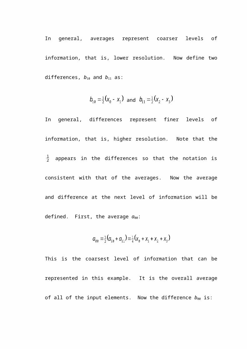
In general, averages represent coarser levels of information, that is, lower resolution.

Now define two differences, b10 and b11 as:

and

In general, differences represent finer levels of information, that is, higher resolution.

Note that the appears in the differences so that the notation is consistent with that of

the averages. Now the average and difference at the next level of information will be

defined. First, the average a00:

This is the coarsest level of information that can be represented in this example. It is

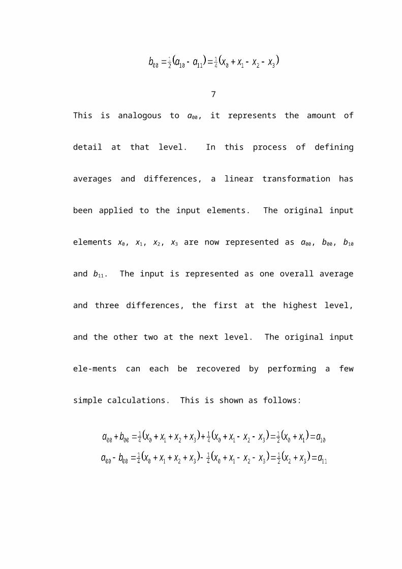
the overall average of all of the input elements. Now the difference b00 is:

7This is analogous to a00, it represents the amount of detail at that level. In this process

of defining averages and differences, a linear transformation has been applied to the

input elements. The original input elements x0, x1, x2, x3 are now represented as a00,

b00, b10 and b11. The input is represented as one overall average and three differences,

the first at the highest level, and the other two at the next level. The original input

ele-ments can each be recovered by performing a few simple calculations. This is

shown as follows:

The sum of the average and difference at level 0 is taken which results in a10, one of

the averages at level 1. The difference of the average and difference at level 0 is

taken which results in a11, the other of the averages at level 1. These averages, along

with the differences at level 1 are used in the next step, which will recover the input

elements.

Sums and differences of the averages and differences at level 1 are taken and all four

input elements are recovered. The averages and differences a00, b00, b10 and b11

provide a lossless representation of the input elements x0, x1, x2, x3, that is, no

information is lost in the process. All original input elements can be exactly

recovered.

8

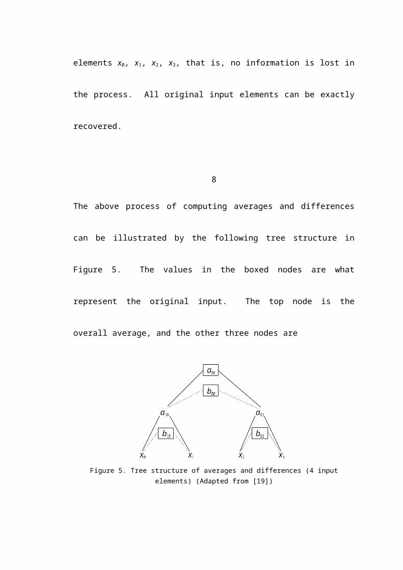
The above process of computing averages and differences can be illustrated by the

following tree structure in Figure 5. The values in the boxed nodes are what represent

the original input. The top node is the overall average, and the other three nodes are

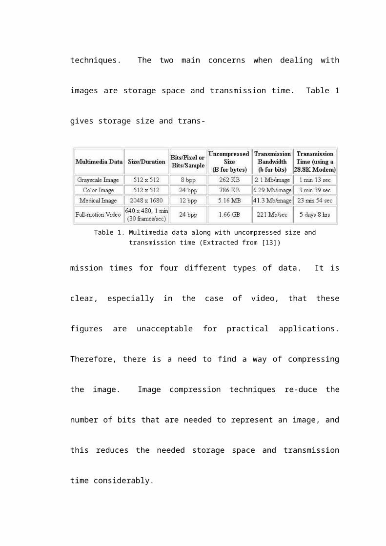
Figure 5. Tree structure of averages and differences (4 input elements) (Adapted from [19])

the differences at each of the two levels. A note about the subscript scheme: for a

node aij or bij, the i represents the level in the tree (0 at the top), and the j represents

the index at level i (i.e., the elements at level i are ordered). The averages at each

inter-mediate level are used to compute the averages and differences at the next

highest level in the tree. The differences at each intermediate level are not used;

calculations stop at those points. The process is iterated until the final overall average

is obtained, that is, the top of the tree is reached.

3.2. Convolution

Another fundamental concept is that of a filter. A filter is a linear time-invariant op-

erator [19]. Time-invariant means that if an input sequence is delayed by t units, then

the output is unchanged, but also delayed by t units, for any value of t. The filter

takes an input vector x and performs a convolution operation of x with some fixed

vector h, which results in an output vector y. This section explains this convolution

process.

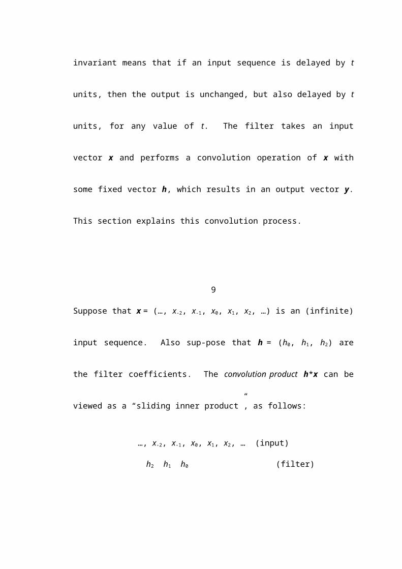
9Suppose that x = (…, x-2, x-1, x0, x1, x2, …) is an (infinite) input sequence. Also sup-

pose that h = (h0, h1, h2) are the filter coefficients. The convolution product h*x can

be viewed as a “sliding inner product”, as follows:

…, x-2, x-1, x0, x1, x2, … (input) h2 h1 h0 (filter)

The inner product between the three lined up components is calculated, then the filter

slides one component to the right, so that it is lined up with the input components with

subscripts –1, 0, and 1. The process is repeated for the entire input sequence. The

convolution product is then:

(…, h0x0+h1x-1+h2x-2, h0x1+h1x0+h2x-1, h0x2+h1x1+h2x0, …, h0xn+h1xn-1+h2xn-2, …)

In general, the nth term can be written in a more compact form as:

(2)

To better illustrate the convolution product computation, a concrete example is now

shown.

Let x = (1, 2, 3) and let h = (2, 1, 5). The first step of the convolution is illustrated as

follows:

1 2 3 5 1 2

In the first step, the right-most filter coefficient is lined up underneath the left-most

input element and the convolution product is calculated. In the places where the filter

coefficients are not underneath any input elements, the input is considered to be 0. In

the second step, the filter shifts right one component, and the convolution product is

calculated again. The filter shifts until its left-most component is lined up underneath

10

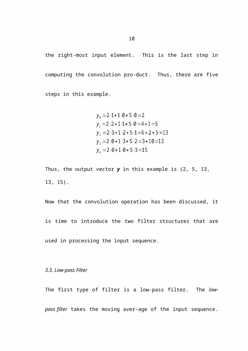
the right-most input element. This is the last step in computing the convolution pro-

duct. Thus, there are five steps in this example.

Thus, the output vector y in this example is (2, 5, 13, 13, 15).

Now that the convolution operation has been discussed, it is time to introduce the two

filter structures that are used in processing the input sequence.

3.3. Low-pass Filter

The first type of filter is a low-pass filter. The low-pass filter takes the moving aver-

age of the input sequence. The simplest type of low-pass filter takes the average of

two components at a time, namely, the input xn at the current time n, and the input xn-1

at the previous time n 1. This is shown by the following equation:

(3)

This can also be represented using matrices:

11

When an input sequence passes through a low-pass filter, the low frequencies pass

through and the high frequencies are blocked. In the words of [19], it “smooths out

the bumps.” A low frequency means that there are fewer oscillations in the input se-

quence. An input of the lowest frequency (0) is a constant sequence, that is, all ele-

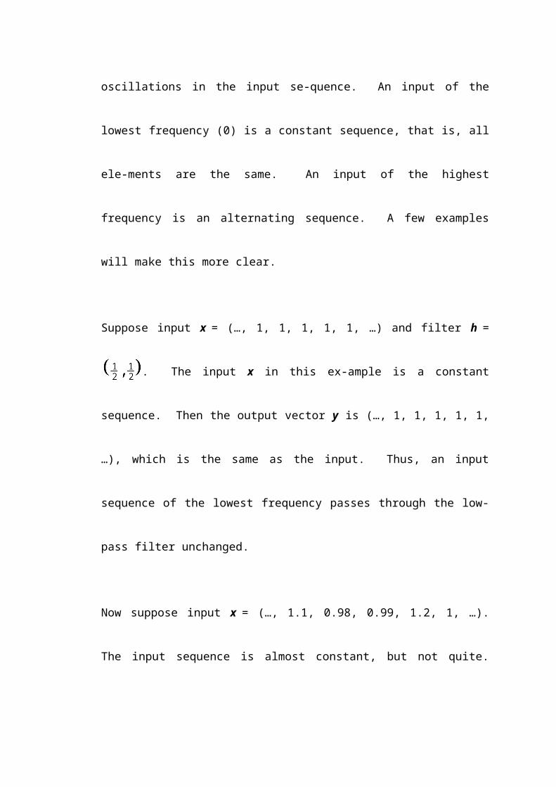
ments are the same. An input of the highest frequency is an alternating sequence. A

few examples will make this more clear.

Suppose input x = (…, 1, 1, 1, 1, 1, …) and filter h = . The input x in this ex-

ample is a constant sequence. Then the output vector y is (…, 1, 1, 1, 1, 1, …), which

is the same as the input. Thus, an input sequence of the lowest frequency passes

through the low-pass filter unchanged.

Now suppose input x = (…, 1.1, 0.98, 0.99, 1.2, 1, …). The input sequence is almost

constant, but not quite. Using the same filter, the output y is (…, 1.04, 0.985, 1.095,

1.1, …). Thus, the output is also almost constant. An input sequence with a low

frequency (but not the lowest) will pass through with very little change.

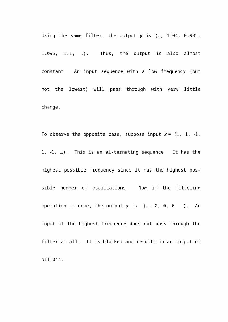
To observe the opposite case, suppose input x = (…, 1, 1, 1, 1, …). This is an al-

ternating sequence. It has the highest possible frequency since it has the highest pos-

sible number of oscillations. Now if the filtering operation is done, the output y is

(…, 0, 0, 0, …). An input of the highest frequency does not pass through the filter at

all. It is blocked and results in an output of all 0’s.

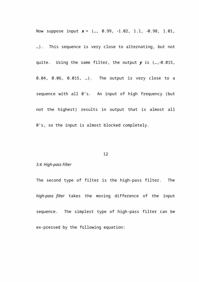
Now suppose input x = (…, 0.99, 1.02, 1.1, 0.98, 1.01, …). This sequence is very

close to alternating, but not quite. Using the same filter, the output y is (…,0.015,

0.04, 0.06, 0.015, …). The output is very close to a sequence with all 0’s. An input

of high frequency (but not the highest) results in output that is almost all 0’s, so the

input is almost blocked completely.

123.4. High-pass Filter

The second type of filter is the high-pass filter. The high-pass filter takes the moving

difference of the input sequence. The simplest type of high-pass filter can be ex-

pressed by the following equation:

(4)

This can also be represented by matrices:

When an input sequence passes through a high-pass filter, the high frequencies pass

through and the low frequencies are blocked. In the words of [19], it “picks out the

bumps.” Again, a few examples will be shown to illustrate the idea.

Suppose input x = (…, 1, 1, 1, 1, …) and filter h = . Performing convolu-

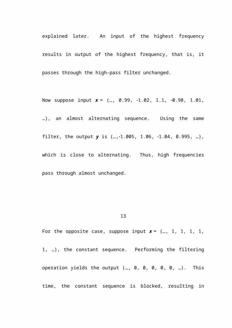
tion results in the output y = (…,1, 1, 1, 1, …). The output is the same as the input,

except it is shifted by one unit, which will be explained later. An input of the highest

frequency results in output of the highest frequency, that is, it passes through the high-

pass filter unchanged.

Now suppose input x = (…, 0.99, 1.02, 1.1, 0.98, 1.01, …), an almost alternating

sequence. Using the same filter, the output y is (…,1.005, 1.06, 1.04, 0.995, …),

which is close to alternating. Thus, high frequencies pass through almost unchanged.

13

For the opposite case, suppose input x = (…, 1, 1, 1, 1, 1, …), the constant sequence.

Performing the filtering operation yields the output (…, 0, 0, 0, 0, 0, …). This time,

the constant sequence is blocked, resulting in output of all 0’s. An input sequence of

the lowest possible frequency does not pass through the high-pass filter at all.

Now suppose input x = (…, 1.1, 0.98, 0.99, 1.2, 1, …), which is close to a constant se-

quence. Using the same filter, the output y is (…,0.06, 0.005, 0.105, 0.1, …), which

is close to all 0’s. Thus, an input sequence that has low frequency is almost blocked

by the high-pass filter.

All of the above discussion on filters has assumed that the operations are done in the

time domain. There are times when it may be desirable to perform the computations

in the frequency domain, rather than the time domain. The next section explains how

this can be done.

3.5. Low-pass and High-pass Filters in the Frequency Domain

Let ω be the frequency of the input, which ranges from 0 (lowest frequency) to π

(highest frequency, i.e. an alternating input sequence). A transformation is done on

the input x = (…, x-2, x-1, x0, x1, x2, …):

A transformation is also performed on the filter h = (…, h-2, h-1, h0, h1, h2, …):

The response y then becomes:

14Y(ω) = H(ω) · X(ω)

Convolution in the time domain corresponds to ordinary multiplication in the fre-

quency domain, since to calculate the output, only a multiplication is needed.

Now the transformation formulas of x and h will be explained. First, recall

DeMoivre’s Theorem:

or (5)

To show the use of these formulas, consider ω = 0. This means that cos 0 + isin 0 =

1 + 0 = 1 which is consistent with the fact that e0 = 1. Now consider ω = π. This

means cos π + isin π = 1 + 0 = 1 (assuming n = 1). Thus, ei π = 1.

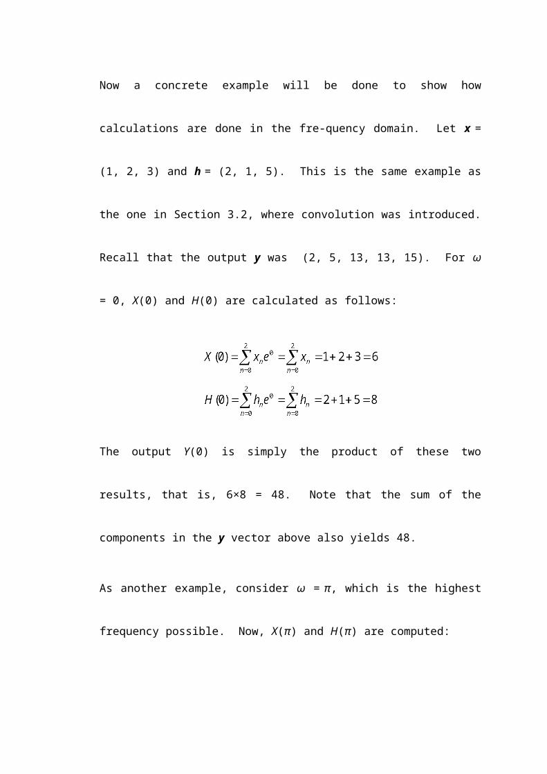
Now a concrete example will be done to show how calculations are done in the fre-

quency domain. Let x = (1, 2, 3) and h = (2, 1, 5). This is the same example as the

one in Section 3.2, where convolution was introduced. Recall that the output y was

(2, 5, 13, 13, 15). For ω = 0, X(0) and H(0) are calculated as follows:

The output Y(0) is simply the product of these two results, that is, 6×8 = 48. Note that

the sum of the components in the y vector above also yields 48.

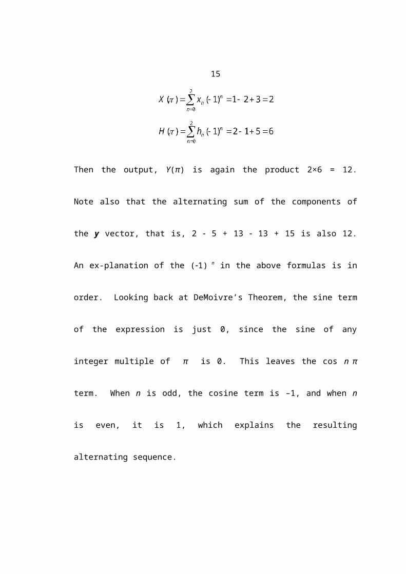
As another example, consider ω = π, which is the highest frequency possible. Now,

X(π) and H(π) are computed:

15

Then the output, Y(π) is again the product 2×6 = 12. Note also that the alternating

sum of the components of the y vector, that is, 2 5 + 13 13 + 15 is also 12. An ex-

planation of the (1) n in the above formulas is in order. Looking back at DeMoivre’s

Theorem, the sine term of the expression is just 0, since the sine of any integer

multiple of π is 0. This leaves the cos n π term. When n is odd, the cosine term is –

1, and when n is even, it is 1, which explains the resulting alternating sequence.

Some amount of computation is saved here, since it is not necessary to perform sev-

eral multiplications, as in the calculation of the convolution product. Only a couple

additions are needed, and just one multiplication at the end. Addition operations are

much faster to perform by computer than multiplication operations.

The subsections that follow explain the operation of the low-pass and high-pass filters

in the frequency domain.

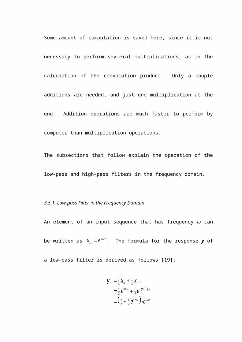
3.5.1. Low-pass Filter in the Frequency Domain

An element of an input sequence that has frequency ω can be written as .

The formula for the response y of a low-pass filter is derived as follows [19]:

16

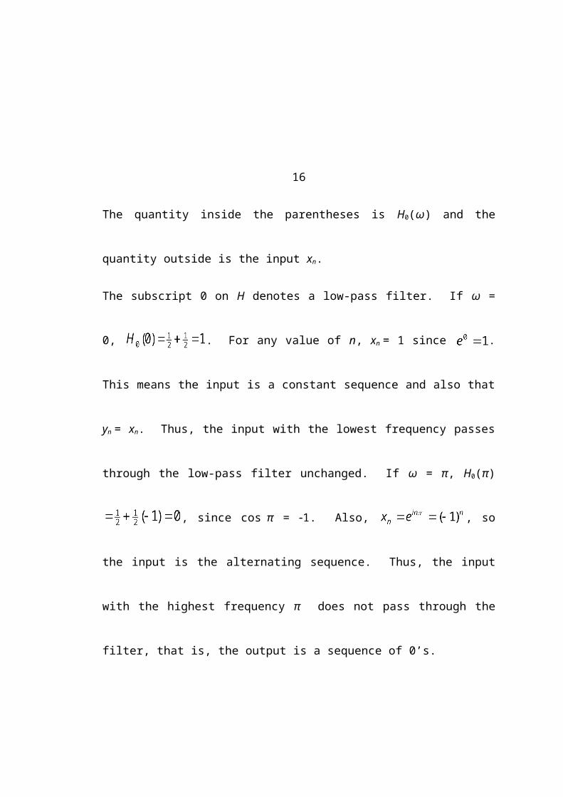
The quantity inside the parentheses is H0(ω) and the quantity outside is the input xn.

The subscript 0 on H denotes a low-pass filter. If ω = 0, . For any

value of n, xn = 1 since . This means the input is a constant sequence and also

that yn = xn. Thus, the input with the lowest frequency passes through the low-pass

filter unchanged. If ω = π, H0(π) , since cos π = 1. Also,

, so the input is the alternating sequence. Thus, the input with the

highest frequency π does not pass through the filter, that is, the output is a sequence

of 0’s.

To show what the filtering function in the frequency domain looks like in general,

consider H0(ω). If is factored out, then H0(ω) becomes:

Recall from DeMoivre’s Theorem that or .

Adding these two equations results in

Thus, where θ . Then the above quantity for H0(ω) can be

written as:

(6)

The cosine term represents the magnitude and the exponential term represents the

phase angle, where the phase is . A plot of the magnitude of H0(ω) is shown in

17

Figure 6. The curve is simply a cosine curve, which is scaled by a factor of . The

0.5 1 1.5 2 2.5 3

0.2

0.4

0.6

0.8

1

H0

Figure 6. Plot of magnitude of H0(ω) (Adapted from [19])

lowest frequency, which is 0, results in a filter value of 1, and the highest frequency,

which is π, results in a filter value of 0. This is consistent with the previous dis-

cussion.

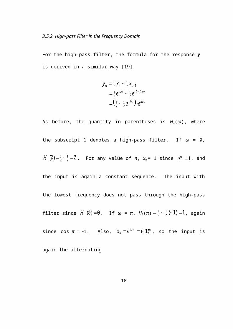
3.5.2. High-pass Filter in the Frequency Domain

For the high-pass filter, the formula for the response y is derived in a similar way [19]:

As before, the quantity in parentheses is H1(ω), where the subscript 1 denotes a high-

pass filter. If ω = 0, . For any value of n, xn = 1 since , and the

input is again a constant sequence. The input with the lowest frequency does not pass

through the high-pass filter since . If ω = π, H1(π) , again

since cos π = 1. Also, , so the input is again the alternating

18

sequence. The input with the highest frequency passes through the high-pass filter

unchanged since yn = xn in this case.

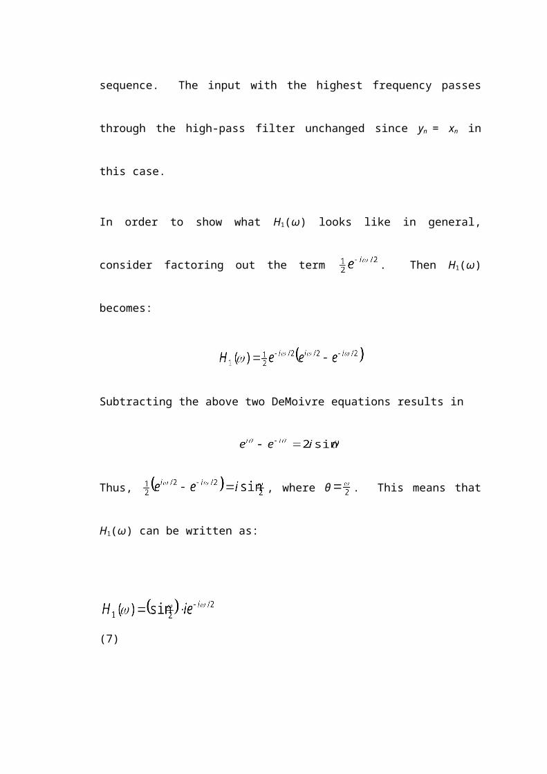
In order to show what H1(ω) looks like in general, consider factoring out the term

. Then H1(ω) becomes:

Subtracting the above two DeMoivre equations results in

Thus, , where θ . This means that H1(ω) can be written as:

(7)

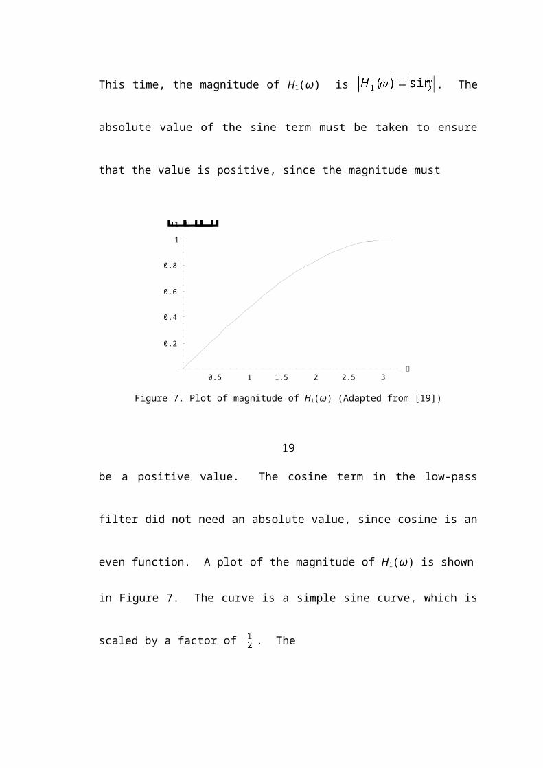
This time, the magnitude of H1(ω) is . The absolute value of the sine

term must be taken to ensure that the value is positive, since the magnitude must

0.5 1 1.5 2 2.5 3

0.2

0.4

0.6

0.8

1

H1

Figure 7. Plot of magnitude of H1(ω) (Adapted from [19])

19be a positive value. The cosine term in the low-pass filter did not need an absolute

value, since cosine is an even function. A plot of the magnitude of H1(ω) is shown

in Figure 7. The curve is a simple sine curve, which is scaled by a factor of . The

lowest frequency value, which is 0, results in a filter value of 0, and the highest fre-

quency value, which is π, results in a filter value of 1. Again, this is consistent with

the above discussion that considers the frequency endpoints.

3.6. Analysis and Synthesis Filter Banks

The low-pass and high-pass filters by themselves are not invertible. This is because

the original input cannot be recovered by applying the inverse transformation of just

one of the filters. The low-pass filter zeros out the sequence (…, 1, 1, 1, 1, …) and

the high-pass filter zeros out the sequence (…, 1, 1, 1, 1, …). There is no way that

these sequences can be recovered from (…, 0, 0, 0, 0, …), since there is no linear

combination of zero vectors that can produce a vector that is non-zero. The solution

to this problem is to use a combination of the two filters, which leads to the discussion

on filter banks.

3.6.1. Introduction

A filter bank is a collection of filters. In this paper, only two types of filters will be

used, low-pass and high-pass. There are two portions of the filter bank that will be

considered, the analysis bank and the synthesis bank. The analysis bank is what per-

forms a linear transformation on the original input by calculating averages and dif-

ferences. The synthesis bank is what recombines the outputs from the analysis bank

to recover the original input. These two methods are now discussed.

203.6.2. Analysis Filter Bank

In the analysis bank, the input sequence is separated into two frequency bands, low

and high. To make the computations easier, the normalization factor must be

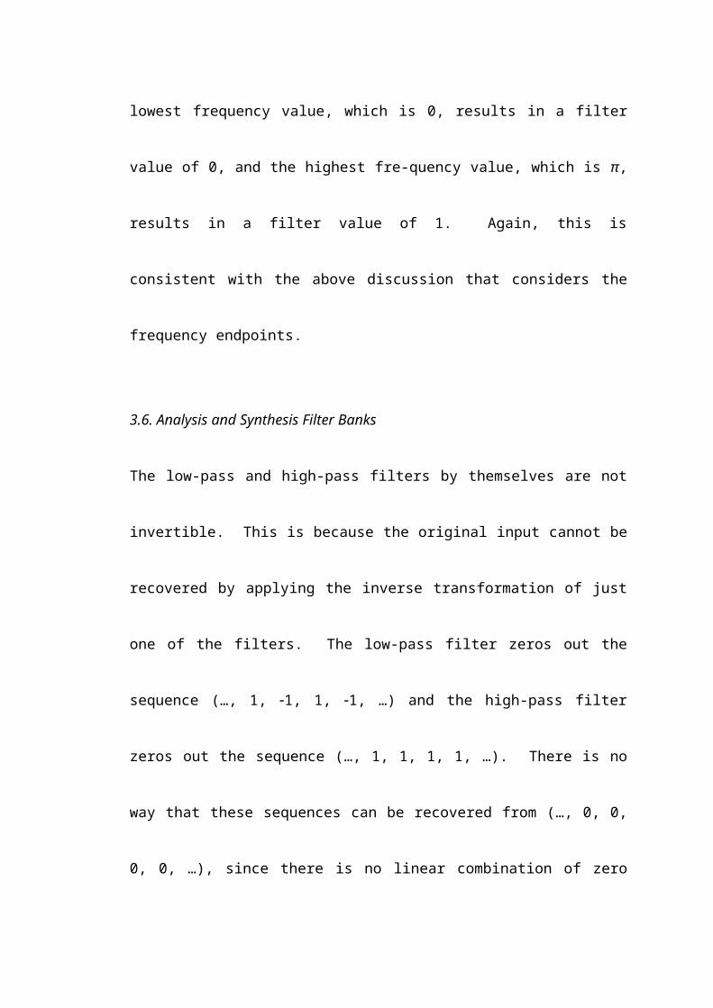
used. This will be explained later. The filter coefficients and are multiplied by

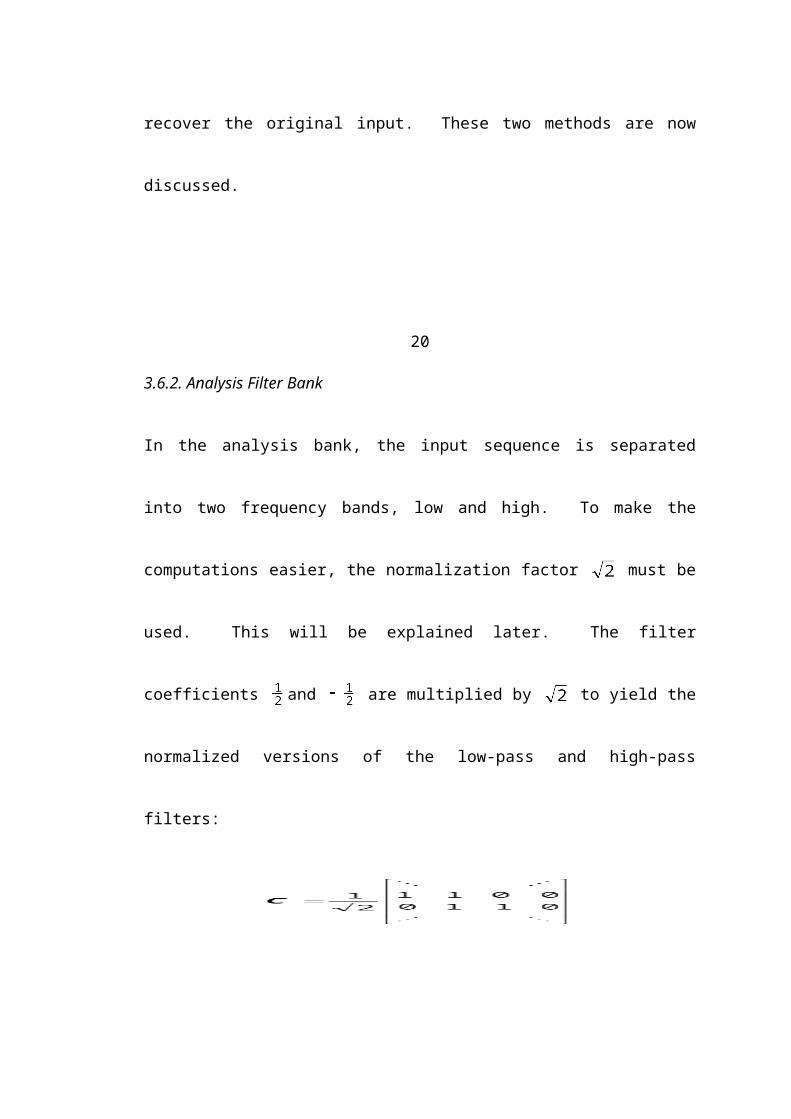
to yield the normalized versions of the low-pass and high-pass filters:

Since the input is split into two sequences, the length has now been doubled. In terms

of storage, this is certainly not acceptable. The solution to this problem is to use a

method called downsampling. Using this approach, the even indexed elements are

kept, while the odd indexed elements are eliminated.

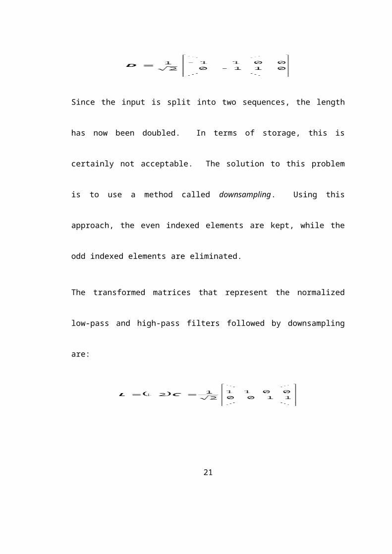
The transformed matrices that represent the normalized low-pass and high-pass filters

followed by downsampling are:

21

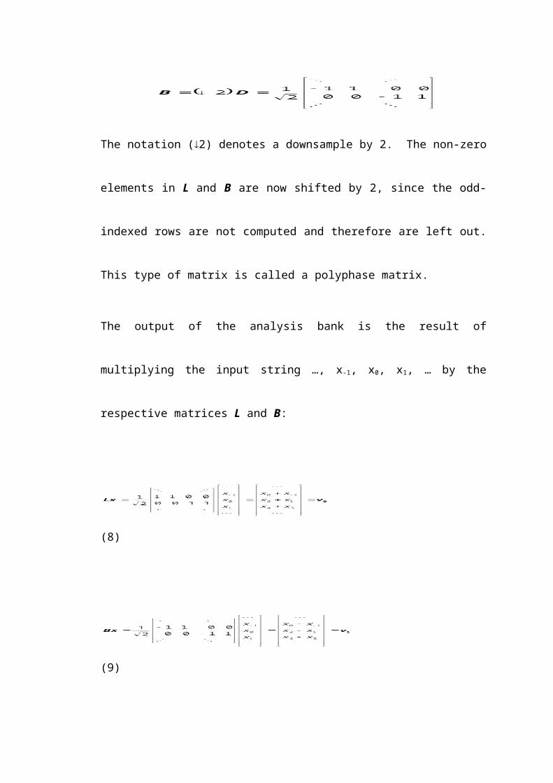
The notation (2) denotes a downsample by 2. The non-zero elements in L and B are

now shifted by 2, since the odd-indexed rows are not computed and therefore are left

out. This type of matrix is called a polyphase matrix.

The output of the analysis bank is the result of multiplying the input string …, x-1, x0,

x1, … by the respective matrices L and B:

(8)

(9)

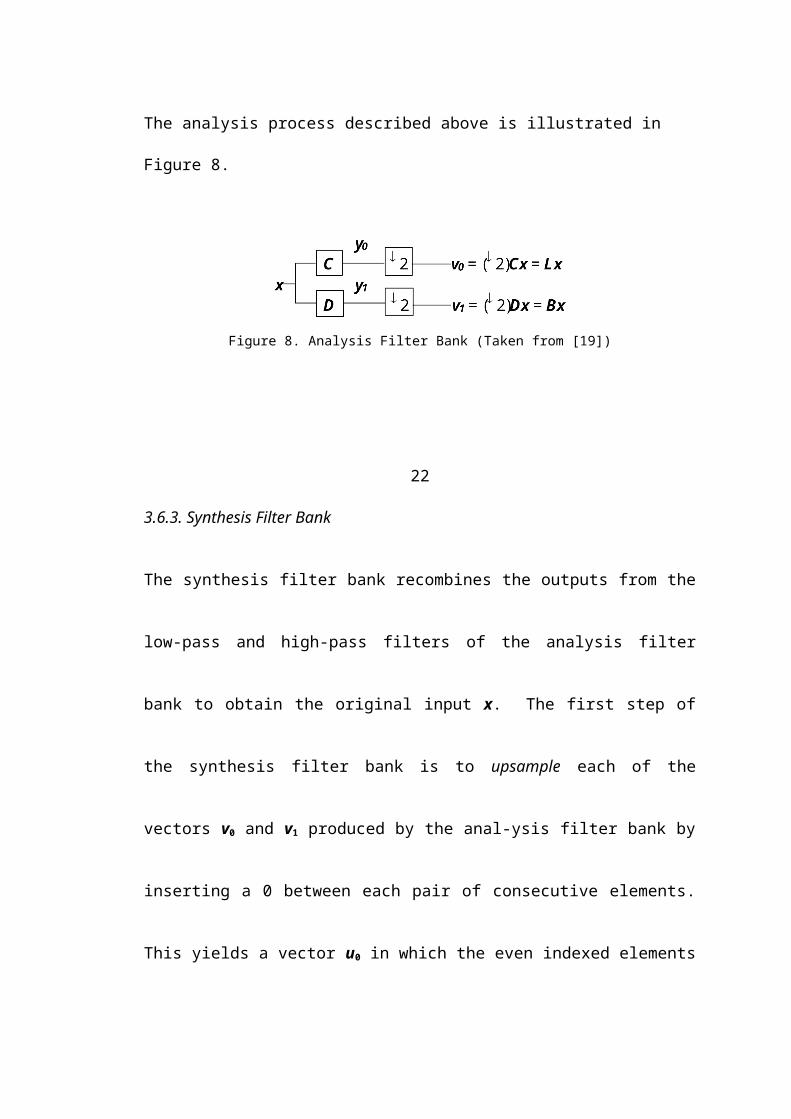
The analysis process described above is illustrated in Figure 8.

Figure 8. Analysis Filter Bank (Taken from [19])

223.6.3. Synthesis Filter Bank

The synthesis filter bank recombines the outputs from the low-pass and high-pass

filters of the analysis filter bank to obtain the original input x. The first step of the

synthesis filter bank is to upsample each of the vectors v0 and v1 produced by the anal-

ysis filter bank by inserting a 0 between each pair of consecutive elements. This

yields a vector u0 in which the even indexed elements are the elements of v0 and the

odd indexed elements are 0. The vector u1 is obtained in the same manner from v1.

and

The upsampling process makes room for the missing elements that were eliminated

during downsampling. The vectors v0 and v1 were only “half-size”, now they are

embedded in vectors u0 and u1 of “full-length.”

The next step is to replace each of the 0’s in the odd indexed positions of u0 with the

vector element immediately preceding it and to replace the scalar multiplier with

.

23

The linear transformation u0→w0 is effected by applying a filter F with coefficients

and . That is,

where is the element in position n of u0.

If n is even, then and . Thus

If n is odd, then and . Thus

The reader can check that for n = 0, 1, …, 5 this yields the elements of the vector w0

given above.

In an analogous manner the vector u1 is transformed to the vector w1,

24

by applying a filter G with coefficients and , as is now shown. The filter G is

defined by

If n is even, then and . Thus

If n is odd, then and . Thus

Again the reader can easily check that for n = 0, 1, …, 5 this gives the elements of the

vector w1 displayed above.

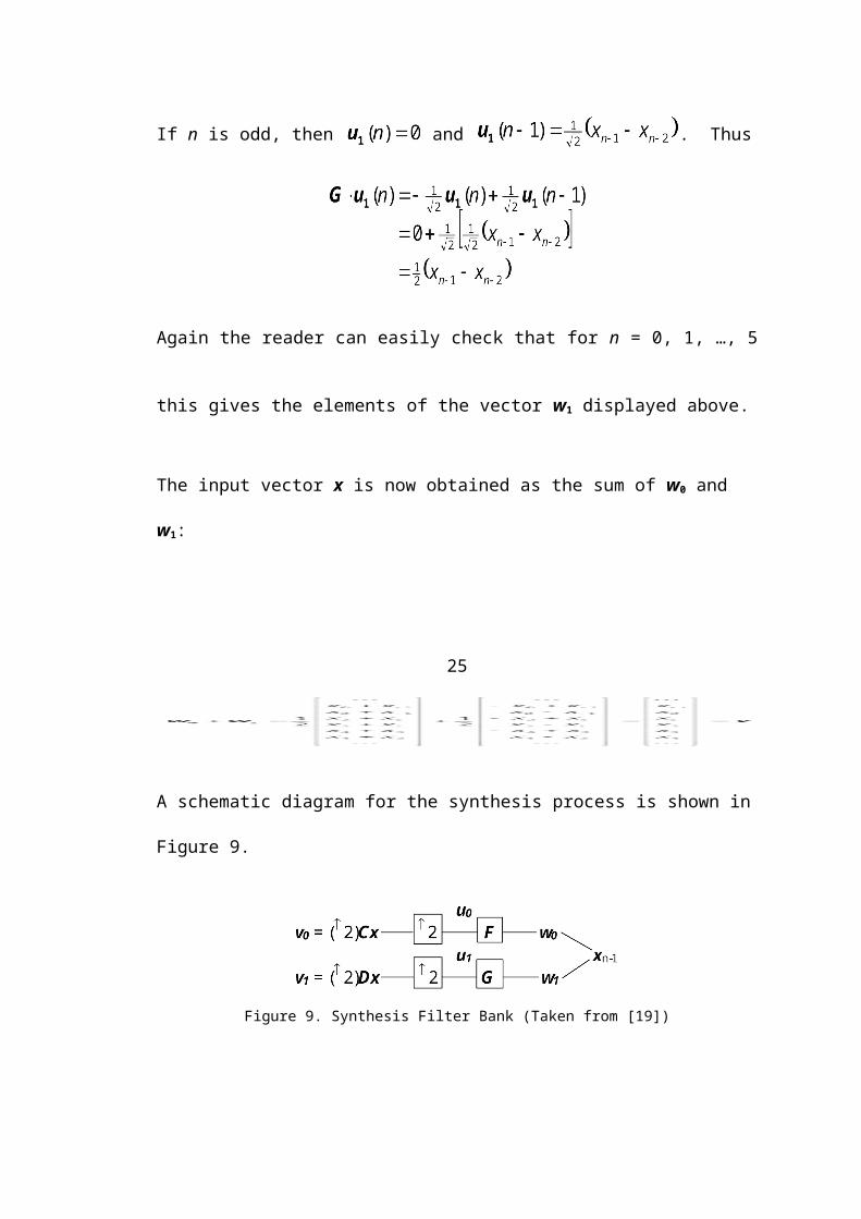
The input vector x is now obtained as the sum of w0 and w1:

25

A schematic diagram for the synthesis process is shown in Figure 9.

Figure 9. Synthesis Filter Bank (Taken from [19])

Note that the recovered input is delayed by one unit. The reason for this is causality.

In order to ensure that output does not come before input, there is a time delay of one

unit.

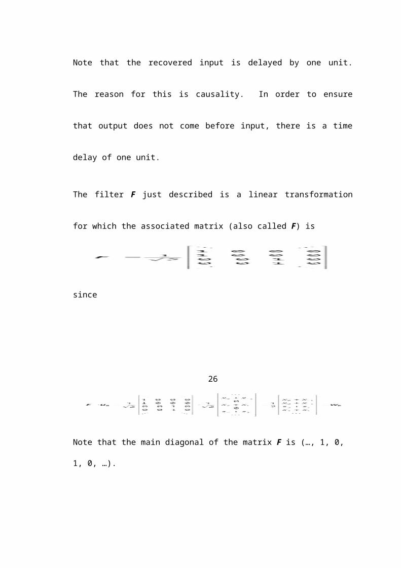
The filter F just described is a linear transformation for which the associated matrix

(also called F) is

since

26

Note that the main diagonal of the matrix F is (…, 1, 0, 1, 0, …).

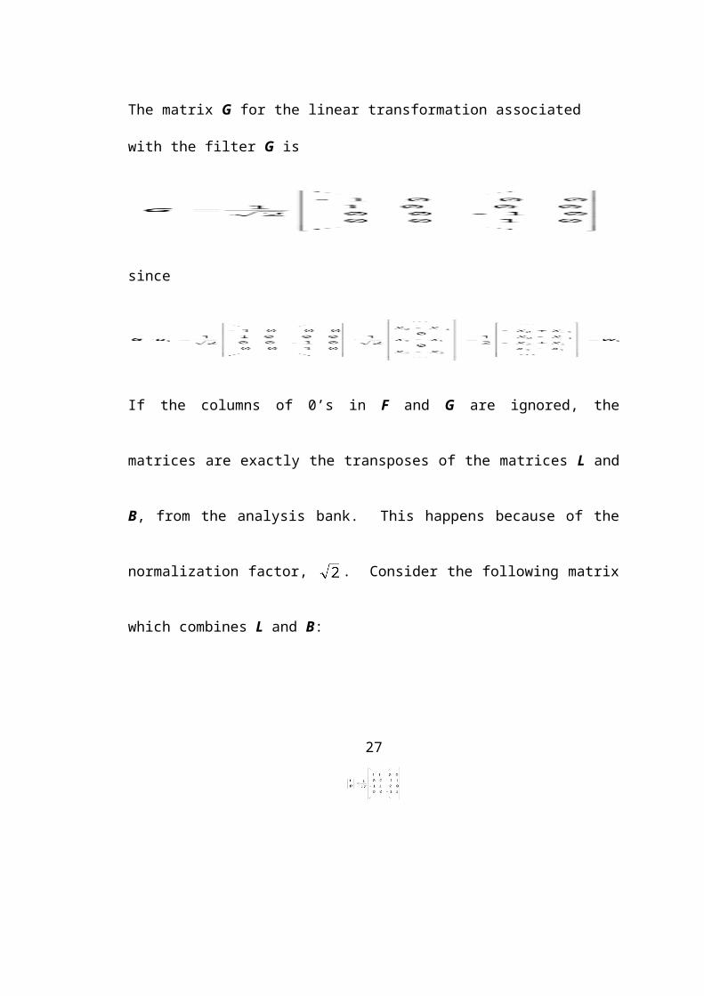
The matrix G for the linear transformation associated with the filter G is

since

If the columns of 0’s in F and G are ignored, the matrices are exactly the transposes

of the matrices L and B, from the analysis bank. This happens because of the

normalization factor, . Consider the following matrix which combines L and B:

27

The row vectors are mutually orthogonal, as are the column vectors, since their inner

products are zero. All row and column vectors are also of unit length since

and . Thus, the rows and columns form an ortho-

normal set, which means that the inverse of the above matrix is simply the transpose.

The analog of the above matrix for the synthesis bank is therefore:

This is the reason for using the normalization factor in the analysis and synthesis pro-

cesses. It is then very easy to calculate the inverse matrix: it is simply the transpose.

A schematic diagram showing the entire filter bank is given in Figure 10. In the anal-

Figure 10. Entire Filter Bank (Taken from [19])

ysis stage, the input is processed by the low-pass and high-pass filters to yield output

28

y. This output is then downsampled by 2 to produce v. In the synthesis stage, the

output v from the analysis stage is first upsampled by 2 to produce u. Lastly, u passes

through the inverse low-pass and high-pass filters to yield w, which is combined to

finally recover the input x, except one time unit later.

As an example, consider an input sequence with two elements. The analysis and syn-

thesis processes can be shown as follows:

for the analysis bank

for the synthesis bank

The top half of A contains the low-pass operation and the bottom half contains the

high-pass operation. Note that the matrices A and A-1 are transposes of each other

(they also happen to be equal in this case). Also note that a00 is the overall average

and b00 is the difference.

3.7. Iterative Filtering Process

Filtering is actually an iterative process, and the number of iterations is dependent on

the size of the input string. For an input string with four elements, there are two

passes that the input takes through the filtering process. Figure 11 shows this iterative

process. After the first iteration, the output from the low-pass filter is passed as input

into the second iteration and this new input passes through the low-pass and high-pass

filters. The output from the high-pass filter of the first iteration does not pass into the

next iteration, calculation terminates there. The output from the low-pass filter of the

29

Figure 11. Two pass analysis bank (Taken from [19])

final iteration is the overall average of the original input string. The other three out-

puts are the differences from both the first and the second level. The above schematic

diagram corresponds to the tree structure previously shown in Figure 5. The low-pass

output from the last iteration corresponds to the root of the tree. The low-pass output

from the first iteration continues up the tree in the same manner as it continues into

the second iteration of the filter bank. The differences, denoted in the tree as b’s, cor-

respond to the output from the filter banks that is not carried into the next iteration.

This process can also be shown as operations of matrices:

The factor s is the normalization factor, which is . The above matrix calculation

shows the analysis process. The matrix A contains averages and differences at both

levels of the filter bank. This is referred to as multiresolution, since different levels of

detail, that is, resolution, are represented. A normalization factor of is needed

in the first two rows of the operator matrix A. This is to ensure that the first two rows

have unit length. Without this factor, the vector length would be

30

, so multiplying by this factor will make the vector length be 1. The synthe-

sis process for four input elements is shown below:

For an input sequence of 8 elements, three passes through the filter banks are

required. Figure 12 shows this process. As before, outputs from low-pass filters are

passed as

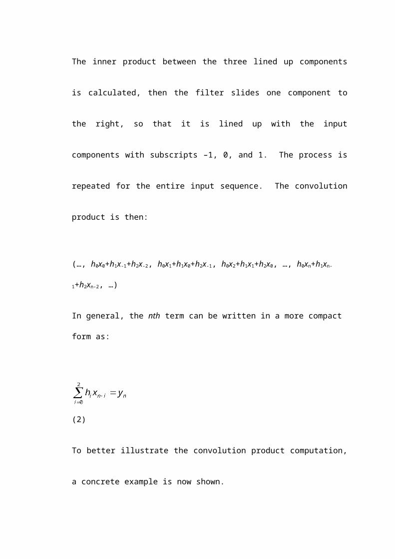
Figure 12. Three pass analysis bank (Adapted from [19])

inputs into the next iteration, and outputs from high-pass filters stay where they are.

The process repeats until the final average, and the 7 differences are obtained. The

corresponding tree structure is given in Figure 13.

31

Figure 13. Tree structure for filter bank with 8 input elements (Taken from [19])

The operator matrix A, for the analysis process with 8 input elements is:

The first row corresponds to a00, the second row to b00, the next two rows correspond

to the differences at level 1, and the last four rows correspond to the differences at

level 2. Note the third power of the normalizing factor in the first two rows of the

matrix. If there are non-zero elements in a row of the matrix, then each element of

that row must be multiplied by to ensure that the row has unit length.

323.8. Fast Wavelet Transform

The matrix multiplications in Section 3.7 involving the analysis matrix A can be done

faster using a factorization technique. Consider the matrix A that operates on an input

string of length 4:

This matrix can be factored as follows:

This factorization can also be written in block form:

The scheme for this factorization will be explained in a moment. First consider the

analysis matrix that operates on an input string of length 8, which is given above. The

factorization of A is as follows:

33

The block form of this factorization is:

An explanation of this factoring scheme follows. Suppose the number of elements in

the input sequence is L = 2J. There are J matrices in the factorization of A. There are

two non-zero entries in each row of the right-most matrix since two coefficients are

used in the filter. If a filter has T coefficients, then there are T×L non-zero entries in

the right-most matrix. The top half consists of the low-pass operation, and the bottom

half consists of the high-pass operation. The next matrix to the left has TL/2 non-zero

entries, which are all in the top half. This does not count the 1’s in the bottom half

since they do not cost anything in the multiplication process. The next matrix to the

left consists of TL/4 non-zero entries, and this pattern continues for each matrix to the

left. The total number of entries in all of the matrices, and therefore the total number

of multiplications t is:

34

(10)

For example, if a filter has two coefficients and the input string has 4 (=22) entries, the

value t is . For an input string with 8 (=23) entries, the value t is

. Since ,

.

Again, t is the total number of multiplications, T is the number of filter coefficients,

and L is the size of the input string. What this means is that the transformation can be

done in linear time. The time it takes is proportional to the size of the input string.

This is the reason why the transformation is referred to as the fast wavelet transform.

Without the factorization, the transform has complexity θ(nlgn). This is a significant

improvement in the required computation time. Note that the time complexity of the

Fast Fourier Transform is θ(nlgn).

The factorization for the synthesis matrix is the inverse of that for the analysis matrix,

as expected. The synthesis matrix factorizations in block form of an input string with

4 elements and with 8 elements are shown below:

for 4 element input string

35

for 8 element input string

This concludes the section on filtering operations. The next section will discuss the

wavelet function and transformation, for both Haar and Daubechies wavelets.

36

4. Wavelet Transformation

4.1. Introduction to Haar Wavelets

The first type of wavelets that were discovered are now known as the Haar wavelets,

named after Alfred Haar [7] who introduced them in 1910. The term wavelet actually

came much later through applications to geophysics. It comes from the French words

onde (wave) and ondelette (small wave). Haar wavelets are an appropriate place to

begin since they are the prototype for all wavelets that have subsequently been dev-

eloped. This means that the iterative process by which the moving averages and dif-

ferences of adjacent terms in the input sequence lead to the Haar wavelets is the same

process that is used to obtain other wavelets. The generalization is obtained by re-

placing the low-pass filter which has coefficients and the high-pass filter which

has coefficients with more complex filters that take weighted averages and

differences of more than two terms in the input sequence. The main goal in digital

signal processing is always to find the "best" filter. In a later section, wavelets known

as Daubechies wavelets will be briefly discussed. These wavelets can be character-

ized as orthonormal functions whose corresponding low-pass and high-pass filters

have the flattest possible frequency response curves for a given filter length at the res-

pective frequencies of 0 and π.

4.2. Scaling Function and Equations

The scaling function, or box function, has the value 1 on the interval [0,1) and

the value 0 for all other real values of t. That is,

(11)

37Its graph is shown in Figure 14.

Figure 14. Scaling function

The octave functions of are the functions for j = 0, 1, 2,.... Their trans-

lations that are of interest are the functions for k = 0, 1, 2,..., . For j

= 1, the two functions are:

and

The graphs of these functions are given in Figures 15 and 16.

Figure 15. Scaling function Figure 16. Scaling function

For j = 2, the four functions are:

38

Their graphs are given in Figures 17-20.

Figure 17. Scaling function Figure 18. Scaling function

Figure 19. Scaling function Figure 20. Scaling function

An easy way to verify the correctness of these graphs is to show that the discont-

inuities occur at the indicated values of t. For example, in the graph of ,

note that when and when .

The graphs given in Figures 14-16 above show that

(12)

This equation is called the dilation equation. This equation, along with its generaliz-

ations, will play a key role in what will follow.

39The graphs in Figures 15-20 above show that

and

Note that these last two equations can be obtained from the dilation equation by re-

placing t by 2t and 2t 1, respectively. Then, replacing t by 2t and 2t 1 in each of

the last two equations yields the following four equations:

It is now easy to note the general dilation equation:

(13)

This equation is valid for all positive integers j and all integers k = 0, 1, …, .

This equation can easily be proved by induction. The proof will not be shown here.

4.3. Wavelet Function and Equations

The other key equation that will play a central role later on, as well as its generaliz-

ations, is the wavelet equation, which is:

(14)

40

The octave dilations of and their translates that are of interest are for

j = 0, 1, 2,... and k = 0, 1, 2,..., .

Repeating the argument given above in deriving the general dilation equation, with

the plus sign changed to a minus sign, yields the general wavelet equation:

(15)

where j is any positive integer and k = 0, 1, 2,..., .

Figures 21-27 below show the graphs of the wavelet functions for j = 0, 1, and 2 and

for all corresponding permissible values of k.

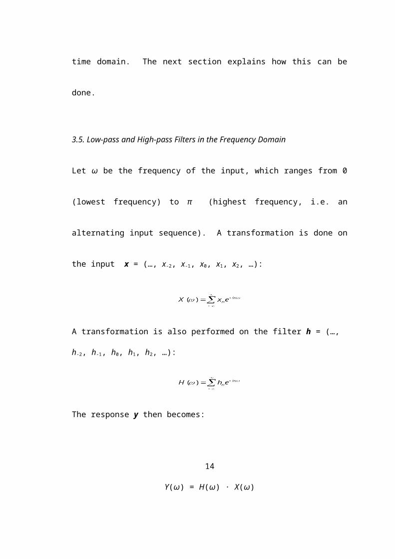
Figure 21. Wavelet function w(t)

41

Figure 22. Wavelet function w(2t) Figure 23. Wavelet function w(2t-1)

Figure 24. Wavelet function w(4t) Figure 25. Wavelet function w(4t-1)

42

Figure 26. Wavelet function w(4t-2) Figure 27. Wavelet function w(4t-3)

4.4. Orthonormal Functions

This section will give several important properties of orthonormal functions.

4.4.1. Inner Product

Recall that the inner product of two n-dimensional real vectors, say x = (a1, a2, …, an)

and y = (b1, b2, …, bn) is

(16)

The generalization of the inner product to real valued integrable functions defined on

some real interval, say [0, 1] is

A function f with domain [0, 1] can be thought of as being an infinite dimensional

vector that has the component value f(t) for each t in the interval [0, 1].

43The two examples above of an inner product are easily shown to satisfy the three con-

ditions:

1. 2. and if and only if f is the zero function3.

for all functions f, g, and h as described above and all real numbers a and b. In fact,

these three conditions are the abstract definition of a real inner product, “real” mean-

ing that is always a real number. An easy consequence of these three proper-

ties is:

4.

for all functions f and g and all real numbers a and b.

4.4.2. Orthonormality

A finite set of real valued functions, say f1, f2, …, fn, with a common domain, say the

interval [0, 1], is orthogonal if

for all i j. (17)

If in addition

for all i (18)

then the set of functions is said to be orthonormal.

It is easy to convert an orthogonal set of functions to an orthonormal set. This can be

44

done by replacing each fi by (1/mi)fi, where mi is the scalar . Then, by

Property 4 of an inner product,

.

Furthermore, if , then , so the

orthogonal property is not affected. The scalar is called the magnitude

of fi. A non-zero function is said to be normalized when it is multiplied by the

reciprocal of its magnitude. Thus, a normalized function f is characterized by having

the property that .

4.4.3. The First Property of Orthonormal Functions: Linear Independence

The first important property of orthonormal functions is that they are linearly indep-

endent. Suppose there are real constants c1, c2, …, cn such that is

the zero function, written as

.

Then taking the inner product of both sides with fi and using the fact that f1, f2, …, fn is

an orthonormal set of functions yields

45

which must be equal to . Hence, each ci = 0, so the orthogonal functions f1,

f2, …, fn are linearly independent.

The way to think about linear independence is that any function has at most one ex-

pression as a linear combination of linearly independent functions. For if

for constants c1, …, cn, d1, … dn, then subtracting yields

Then the linear independence of f1, …, fn implies that c1 = d1, …, cn = dn.

4.4.4. The Second Property of Orthonormal Functions

Now suppose that given a function f, one wants to find constants c1, …, cn (unique if

they exist) such that

where f1, f2, …, fn is an orthonormal set of functions. The method is the same as that

used above to show linear independence; that is, take the inner product of both sides

of the equation with fi to obtain

.

Hence

46This is the second important property of a set of orthonormal functions. The coeffi-

cients ci in are therefore easy to find provided that the integrals

are easy to evaluate. However, one must be careful since f might not be expressible as

a linear combination of the orthonormal set f1, f2, …, fn. Then the above expression

is not true; it was derived under the false assumption that f could be

expressed as . However, can be viewed as the “best” approx-

imation to f that can be obtained using only the functions f1, f2, …, fn.

4.5. The Theory Behind Wavelets

This section will develop the important theory behind the wavelet functions.

4.5.1. The Vector Space of the Scaling Functions

For every positive integer j let be the vector space spanned by the box func-

tions , , , …, . That is, consists of all

functions

,

where and the ak’s are arbitrary real numbers.

The support of a function f(t) is the set of values for t where f(t) is non-zero:

47

By definition, . Hence

(19)

since implies and implies . There-fore,

the supports of

, , , …,

are the respective non-overlapping intervals

which cover the interval [0, 1). Therefore, consists of all step functions which are

constant on each of the subintervals of [0, 1) listed above. Furthermore, the functions

in are zero outside the interval [0, 1). Since these supports are pairwise dis-

joint, a function

in can be the zero function only if all ak’s are zero. Therefore, the set of func-

tions , k = 0, 1,…, are linearly independent. In fact, these func-

tions are orthogonal since the disjointness of the supports of and

for k K implies that their (pointwise) product is the zero function.

48

Hence,

when .

4.5.2. Normalized General Dilation Equation

In order to obtain an orthonormal basis for each function is normalized

by multiplying it by the reciprocal of its magnitude. The support of is an

interval of length on which has the value 1. Therefore,

and hence

Thus the magnitude of is . The functions , (k = 0, 1, …,

) defined by

are therefore an orthonormal basis for .

This expression for the magnitude of is true for all nonnegative integers j

and all corresponding values for k = 0, 1, …, . Thus if j is a positive integer,

then

49

for k = 0, 1, …, . This equation is used to normalize the general dilation

equation

Multiplying the left hand side by and the right hand side by

written in the form yields

(20)

for k = 0, 1, …, .

4.5.2. Normalized General Wavelet Equation

The general wavelet equation

can be normalized in a similar way. The general wavelet equation states that

has the value 1 on the support of and the value –1 on the

support of . Since these two supports are disjoint intervals of length

, has the value 1 on its support which is an interval of length

. Therefore,

.

50

Hence, the function defined by

is the normalization of w(2j–1t – k). It is called a normalized Haar wavelet. Multi-

plying both sides of the general wavelet equation by yields the normalized

general wavelet equation

(21)

where j is a positive integer and k = 0, 1, …, .

4.5.3. The Subspace Spanned by the Scaling and Wavelet Functions

Theorem 1: Let j be a positive integer and let 2k be an even integer satisfying

. Then and span the same 2-dimensional

subspace of as do and . Furthermore, and

are ortho-gonal.

To give an idea of the proof, an example will now be shown, with j = 1.

When j = 1 in Theorem 1, the condition implies that k = 0. Then

and are the functions and whose graphs are shown

in Figures 28 and 29.

51

Figure 28. Scaling function Figure 29. Wavelet function

Similarly, the functions and are and

whose graphs are shown in Figures 30 and 31.

Figure 30. Scaling function Figure 31. Scaling function

The normalized general dilation and wavelet equations for j = 1 and k = 0 are

Since and are expressible as linear combinations of and

52

, the subspace spanned by and is a subspace of the 2-dimen-

sional subspace spanned by and . However,

by inspection of the above graphs. Thus and are orthogonal and hence

linearly independent. Hence, and span a 2-dimensional subspace

which is contained in the 2-dimensional subspace spanned by and .

Therefore, and span the same subspace as and .

The proof of Theorem 1 is in the Appendix.

4.5.4. First Orthonormal Basis for the Vector Space of Scaling Functions

Theorem 2: The union of the two sets of functions

and

is an orthonormal basis for the vector space which has

as an orthonormal basis.

53The proof of Theorem 2 is given in the Appendix.

4.5.5. Second Orthonormal Basis for the Vector Space of Scaling Functions

Theorem 2 was obtained by using Theorem 1 as k runs through the values 0, 1, …,

. Using Theorem 2 as j runs through the values j, j – 1, …, 0, yields Theorem

3. The first application of Theorem 2 to yields as an alternative basis

for . Next, apply Theorem 2 with j replaced by j – 1 to to obtain

as an alternative basis for the subspace spanned by the functions in

, and hence, as an alternative basis for . The process is shown

in Figure 32 below.

Figure 32. Derivation of basis for

This process is analogous to the filtering process in Section 3.7. The operations

represent a low-pass filter operation, and the W operations represent a high-pass filter

operation. The result is the overall average and all of the differences at each level.

Theorem 3. The vector space with orthogonal basis

has another orthonormal basis consisting of the

union of the following set of functions:

54

The proof of Theorem 3 is given in the Appendix.

4.6. The Connection Between Wavelets and Filters

This section will demonstrate the connection between the wavelet theory and the pro-

blem of filtering an input data stream.

The input data string a0, a1, …, aN is identified with the vector (a0, a1, …, aN) in RN+1-

the (N + 1)-dimensional vector space over the real numbers. Also, a0, a1, …, aN is

identified with the function

in the (N + 1)-dimensional vector space that has the orthonormal basis

. This means that the function is identified with the

vector that has all zeros except for a 1 in the first (0 th) position,

is identified with the vector that has all zeros except for

a 1 in the last position. Note that since is an orthonormal

basis for , the inner product which is defined in terms of integrals agrees with the

usual dot product on RN+1 as is shown below. Let

55

and

Then

since

The normalized general dilation equations

for k = 0, 1, …, indicates how to associate a vector in RN+1 with a vector in

RM+1 of half the length by adding adjacent terms. Here and .

For example, if j = 3, then

56

The normalized general wavelet equation

for j = 0, 1, …, gives an alternative way of mapping a vector in RN+1 to a

vector in RM+1. For j = 3,

Theorem 2 gives the result of the first stage of a filter bank for the Haar wavelets

while Theorem 3 gives the result of the entire filter bank for Haar wavelets. These

two theorems together give another proof that the Haar transform is lossless.

4.7. Daubechies Wavelets

Now that the Haar wavelets have been discussed, it is time to develop some theory

behind the Daubechies wavelets.

4.7.1. D4 Wavelets

In this section, the Haar wavelets are generalized to the Daubechies wavelets D4.

These wavelets were discovered by Ingrid Daubechies in 1988 while working at

AT&T Bell Laboratories [4]. This discussion is based on [27], [17], and [18].

The key concept in Haar wavelets is the dilation equation, which in its simplest

(ungeneralized and unnormalized) form is

.

57An obvious generalization would be a dilation equation of the form

,

where the constants are to be determined. The nonzero constant s could

be omitted (i.e. absorbed into the constants ) but its inclusion makes the

derivation somewhat easier. Also, it is best to have an even number of terms in the

dilation equation (this example contains four terms) so that the rows of the high-pass

filter matrix can be made orthogonal to the rows of the low-pass filter matrix. This

makes reconstructing the original data stream from its wavelet transform easier and it

was important in proving Theorems 1 and 2.

In order to not worry about the supports of the resulting wavelet function, it is as-

sumed that the inner product of two functions, say f and g, is defined by

.

The first step is to find a relationship between s and . This is done by

in-tegrating both sides of the dilation equation:

In the last step the substitutions , were made. Canceling the inte-

grals from the first and last terms of these equations yields

58

Now, two normalization assumptions are made. The first is that

and the second is that

Finally, it is assumed that the functions are

or-thogonal; that is, if , then

Note that the counterparts of the above three assumptions are true for Haar wavelets;

in that case there are only two coefficients, , and is the box function.

Here, however, will be a much more complicated function.

The above three assumptions yield

59

Thus, so let . Therefore, the following two conditions on the ci’s are:

(22)

(23)

In analogy to what was done for Haar wavelets, the goal is to modify the dilation eq-

uation to obtain a wavelet equation. Let

Note that this choice makes and orthogonal, which is a crucial property

that was used in proving Theorems 1 and 2 for Haar wavelets. The nonzero terms in

the low-pass filter will be and the nonzero terms in the high-pass filter

will be .

In addition to the two conditions on the four coefficients , two more

conditions are needed. Daubechies’ choice was to have the vectors (1, 1, 1, 1) and

(1, 2, 3, 4) orthogonal to . This yields

(24)

and

60

(25)

The four equations for the ci’s given above have two solution sets; one solution set is:

The other solution set is obtained by replacing each by (and each by

) in the above solution set. Note that changing the sign on reverses the order of

the numbers . The Daubechies wavelets D4, use the values for

from the first solution set, which is an arbitrary choice.

Daubechies’ choice to have the vectors (1, 1, 1, 1) and (1, 2, 3, 4) orthogonal to

was made so that the resulting wavelets would provide good ap-

proximations to horizontal line segments and to line segments with nonzero finite

slope. Perhaps it was a natural choice in view of the difficulty of approximating line

segments that rise or fall rapidly with Haar wavelets; the result is the familiar

“staircase” effect. In retrospect, it was a brilliant choice because of the significant

properties and applications that the Daubechies wavelets are now known to have.

4.7.2. D6 Wavelets

The Daubechies wavelets D6 can be obtained using the dilation equation

and the associated wavelet equation

61

in direct analogy to what was done for D4 (replace the 5’s by 3’s to obtain the pre-

vious equations). The normalization equations for D6 are

and

.

The equations

that resulted from requiring that be orthogonal to (1, 1, 1, 1) and

(1, 2, 3, 4) are generalized to requiring that be

orthogonal to (1, 1, 1, 1, 1, 1), (1, 2, 3, 4, 5, 6) and . The

resulting three equations are called the vanishing of the zeroth, first, and second

moments of respectively.

Suppose that the coefficients of the low-pass filter associated with the

D4 wavelets are offset from themselves at a distance of two:

62The corresponding inner product is:

Consequently, the scaling functions associated with the Daubechies wavelets D4 are

orthogonal; in fact, orthonormal since . The even offset is of course, a re-

sult of the downsampling in the low-pass filter. For the scaling functions associated

with the Daubechies wavelets D6, it is necessary to consider offsets of two and four in

order to guarantee orthogonality:

(26)

(27)

There are now seven sets of equations for the six unknowns . However,

the condition is redundant, it can be obtained as a consequence of the or-

thogonality of the scaling functions as was done for D4.

The graphs in Figures 33 and 34 are for D4 and D6 wavelets respectively.

Figure 33. D4 wavelet (Taken from [27]) Figure 34. D6 wavelet (Taken from [27])

63

These graphs were generated by applying the inverse wavelet transform to a long (e.g.

1024) vector that has all 0’s except for a single entry of 1. For more details, see [27]

and [12].

The coefficients for the D4 and D6 wavelets are shown in Tables 2 and 3.

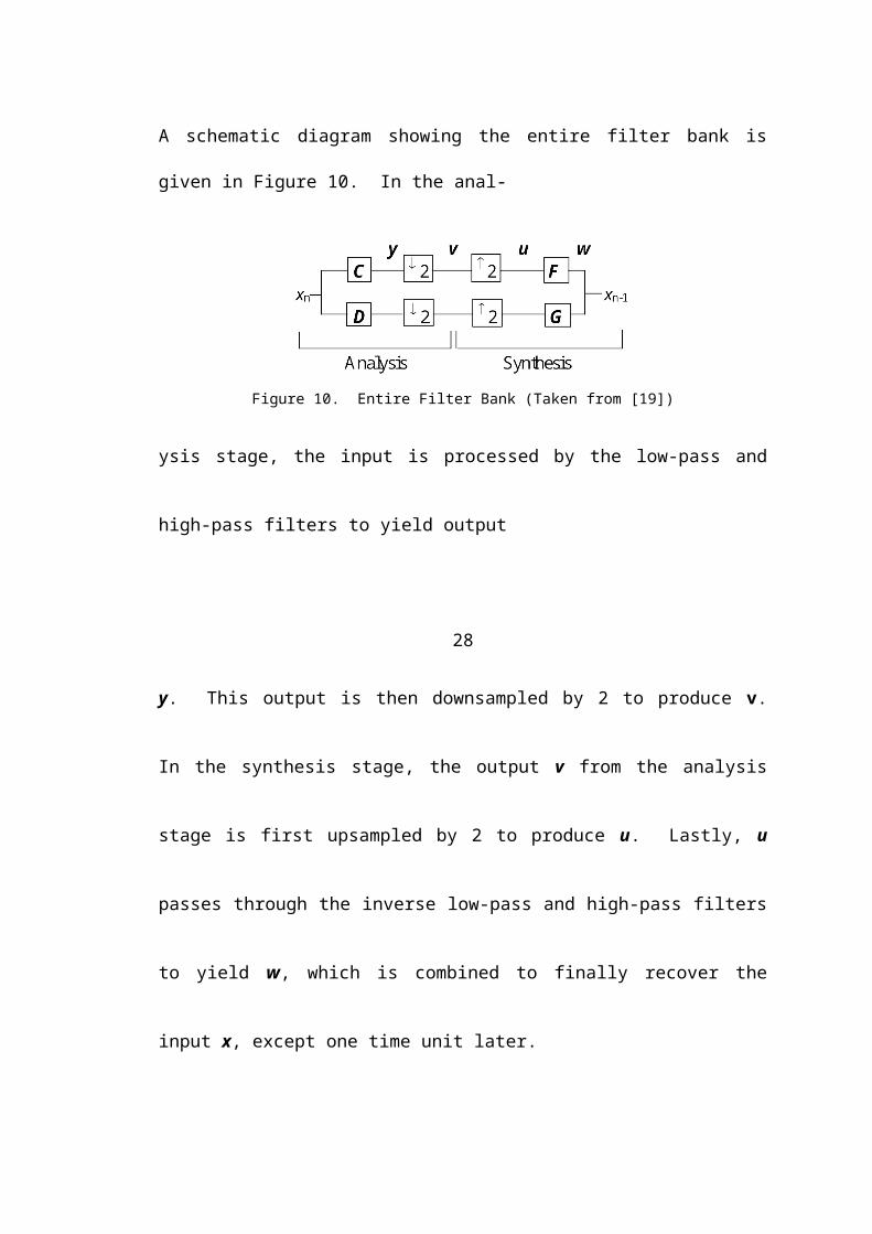
Table 2. Coefficients for D4 Table 3. Coefficients for D6

4.7.3. Flatness

The support of D4 is the interval [0, 3] and for D6 it is [0, 5]. The function D4 is

everywhere continuous but it is not differentiable at points in the interval (0, 3) of the

form , where k and n are integers. At these points, D4 has a left derivative but not

a right derivative. The function D6 and its first derivative are everywhere continuous,

but higher derivatives do not exist. In general, the smoothness of the Daubechies

wavelets depends on the number p of vanishing moments (previously discussed),

gaining about “half a derivative” for each increase in p.

The advantage of the Daubechies wavelets with more coefficients is that the mag-

nitudes of the frequency response curves for the corresponding low-pass and high-

pass filters are “flatter” at the two extreme frequencies of 0 (i.e. a constant input …, 1,

1, 1, …) and π (i.e. an alternating input …, 1, –1, 1, –1, …). These “flatness” con-

ditions are a direct consequence of the vanishing moments conditions, see [19]. The

drastic improvement in flatness from D4 to D24 is illustrated in the following eight

graphs in Figure 35. The first four graphs are for D4 and the last four graphs are for

D24.

64

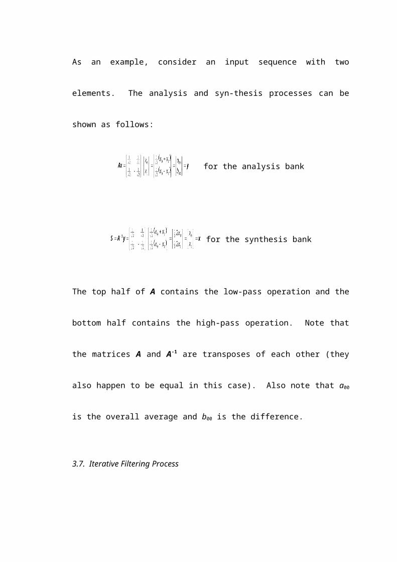
Figure 35. Daubechies graphs showing improvement in flatness (Taken from [19])

65

Here H0(Z) is the magnitude of the frequency response for the low-pass filter (scaling

function) and H1(Z) is that for the high-pass filter (wavelet function).

4.8. Two Dimensional Wavelets

Wavelet transforms in two dimensions are computed by first applying the one

dimensional wavelet transform to the rows of the input matrix, and then applying the

same operation to the columns of the input.

Suppose a 4×4 image is represented as

.

The function that represents this image [27] is given by

where .

(28)

The summation actually represents union rather than summation. The double sum-

mation denotes operating on both the rows and columns.

The wavelet transform on row i is given by

66

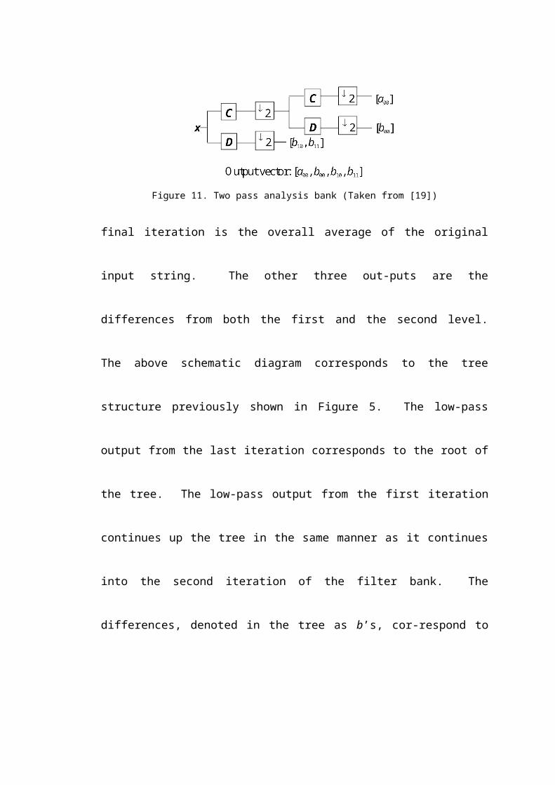
The first term represents the overall average of row i and the other three terms denote

the three differences. This is analogous to the filtering scheme with a one-dimen-

sional input string of length 4.

This formula can be substituted back into the above equation representing the image:

(29)

This represents the transformation on the columns of the image. Each of the terms

denotes the operation on one of the columns.

The wavelet function in two dimensions will then be a cross product of wavelets in

one dimension. Recall the wavelet functions shown in Figures 22 and 23. There are

four possible cross products of these wavelets and their graphs are given in Figures

36-39.

Figure 36. 2D wavelet w(2s) w(2t) Figure 37. 2D wavelet w(2s) w(2t-1)

67

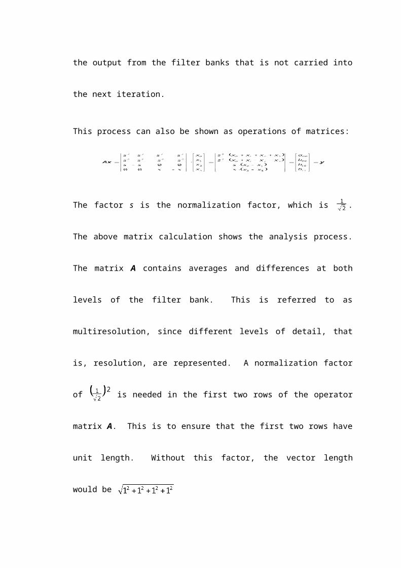
Figure 38. 2D wavelet w(2s-1) w(2t) Figure 39. 2D wavelet w(2s-1) w(2t-1)

The graphs are actually three dimensional. The values in each of the squares repre-

sent the height or amplitude of the function. The amplitude can be 1, –1, or 0 on each

of the 16 subregions of the graph. These magnitudes are represented by the symbols

+, –, and 0 respectively. In Figure 36, the graph of w(2s) w(2t) is shown. In the

graph of w(2t), the graph has positive amplitude in the interval [0, ) so a + appears in

the bottom left square. The graph of w(2t) has a negative amplitude in the interval [ ,

), and this results in a + in that region since (1) (1) = 1. The two squares with a –

are where the function has positive amplitude in one interval, and negative amplitude

in the other. The other three graphs are produced in the same manner.

This concludes the material on the Haar and the Daubechies wavelets. The next sec-

tion will present the actual image compression techniques.

68

5. Image Compression Using Wavelets

In 2000, JPEG introduced a new standard, JPEG2000 which uses wavelets to trans-

form the image instead of earlier methods such as the Discrete Cosine Transform.

The wavelet transform of images and the image compression algorithm will be dis-

cussed in this section.

5.1. Wavelet Transform of Images

Since images have two dimensions (height and width), image compression techniques

that use wavelets use two-dimensional wavelets. Filter operations are first performed

on the rows of the image, then filter operations are performed on the columns of the

row-transformed image. This process can be iterated several times. At each iteration,

a different level of resolution is represented. The end result contains several different

levels of detail, that is, several different scales of resolution. At each level, all four

combinations of low-pass and high-pass filters used on rows and columns of the

image are performed. In Figure 40, the first level of resolution is shown. Each corner

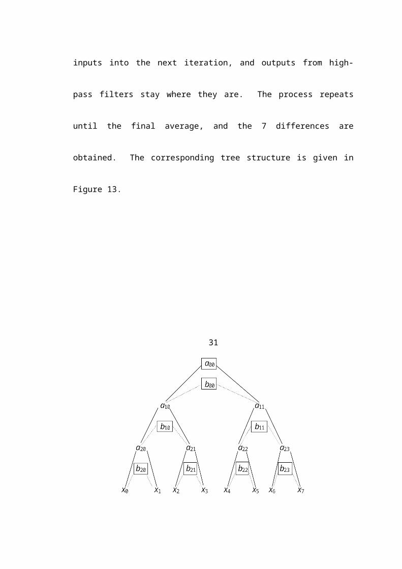
Figure 40. One level decomposition

69consists of one of the combinations mentioned above. The symbols are interpreted as

follows: LL1 means a low-pass filter operates on the rows, then a low-pass filter op-

erates on the columns; HL1 means a high-pass filter operates on the rows, then a low-

pass filter operates on the columns; LH1 means a low-pass filter operates on the rows,

then a high-pass filter operates on the columns; and HH1 means a high-pass filter op-

erates on the rows, then a high-pass filter operates on the columns. The subscript of 1

on each symbol indicates the level of decomposition, in this case it is the first level.

As a concrete example, consider the house image in Figure 41. Its one level decom-

Figure 41. House example (Taken from [23])

Figure 42. One level decomposition of house example (Taken from [23])

70position is given in Figure 42. The upper left corner contains a smaller version of the

original. This is the result of taking averages of both the rows and the columns. A

more blurred version of the image results since averages are taken using low-pass fil-

ters. The constant regions pass through, while the more detailed areas, that is, the

edges, are blocked. The image is shrunk to one-fourth of its original size since the

first filter results in half as many columns and the second filter results in half as many

rows. The upper right corner of the decomposition represents the vertical edges of the

image. Applying a high-pass filter across a row results in picking up details between

adjacent pixels, and as the filter moves down to subsequent rows, it results in the ver-

tical edges being revealed. There is not much change along an edge and so applying a

low-pass filter down a column preserves vertical edges. In an analogous manner, the

lower left corner represents the horizontal edges. The lower right corner contains co-

efficients representing the edges that are diagonal, since differences are preserved in

both the horizontal and the vertical direction.

This process is repeated on the upper left corner which is the one labeled LL1. The

other three corners are left as they are. This is analogous to the filtering process des-

cribed in Section 3.7. The three corners that are left alone were computed using at

least one high-pass filter and they represent the detail in the image at that level. The

upper left corner was computed using only low-pass filters. The process can be re-

peated on each successive LL corner as many times as desired or until the image can-

not be further decomposed; at that point, the last LL corner represents one value, the

overall average of the original image.

In Figure 43, the decomposition for three levels is shown.

71

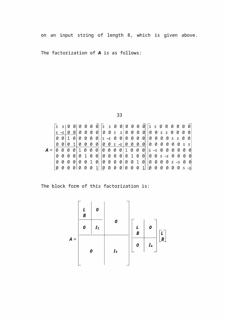
Figure 43. Three level decomposition

Figure 44 shows this decomposition on the house image example. The decomposition

now represents three levels of detail of the image. This is what is meant by multi-

resolution.

Figure 44. Three level decomposition of house example (Taken from [23])

Each level represents coarser and coarser levels of detail. The finest details are given

72

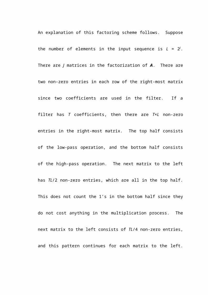
in the three quadrants HL1, LH1, and HH1. The upper left corner keeps getting smaller

after each iteration. It is analogous to a person moving farther and farther from an ob-

ject, and eventually the object simply appears as a blur, which is one uniform value,

the overall average.

The corresponding filter diagram for decomposition at three levels in given in Figure

45.

Figure 45. Filter diagram for three iterations of two-dimensional wavelet

Again, each level is composed of two parts; the first operation is on the rows, and the

second is on the columns. Results from applying a high-pass filter are left as they are

and the result of the LL operation is passed into the next iteration.

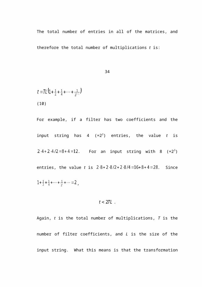
73

To show what is happening in terms of matrices and internal operations on coeffi-

cients, an example will now be given. Consider the image in Figure 46:

Figure 46. Example image used for calculating decomposition (Adapted from [10])

Each of the small squares represents one pixel of the image. The array containing the

gray level values is given by:

The values are different than they are in [10]. They have been scaled so that they are

in the range 0-255, where 0 is black and 255 is white. The value for each pixel repre-

sents how light or dark that pixel is in terms of gray level. The range 0-255 is com-

monly used.

74Now the three level decomposition will be calculated step by step. First, the bands at

the first level LL1, HL1, LH1, and HH1 are computed. The operations will be done left

to right, for example, in calculating HL1, first a high-pass filter is applied to the rows

then a low-pass filter is applied to the columns of the resulting matrix.

The result of applying a high-pass filter to the rows of the original matrix is given by:

The high-pass filter matrix is identical to the downsampled matrix in the previous dis-

cussion in Chapter 3 except that this matrix is actually the transpose of the matrix in

that section. This is because the input string in the former section was treated as a

column vector, whereas here, input is treated as row vectors. The operation is still the

same; the difference of every two pixel values in taken for each of the eight rows.

This results in the size of each row reducing by half, that is, the number of columns is

now half of what it was in the original matrix. Note that the normalization factor is

omitted in this example for simplicity. Also, values have been rounded to be conven-

ient integer values.

To compute the HH1 band, a high-pass filter is now applied to the columns of the re-

sulting matrix from the previous step:

75

The filter used here is the transpose of the filter used in the previous step, and this

time, it is multiplied on the left rather than the right. This is to ensure that the matrix

HH1 has the proper dimensions, four rows and four columns. The computation is ana-

logous to the one above. The difference of every two elements in each column is

taken, which results in the number of rows reducing by half. The final matrix HH1

has a size that is one-fourth of the original.

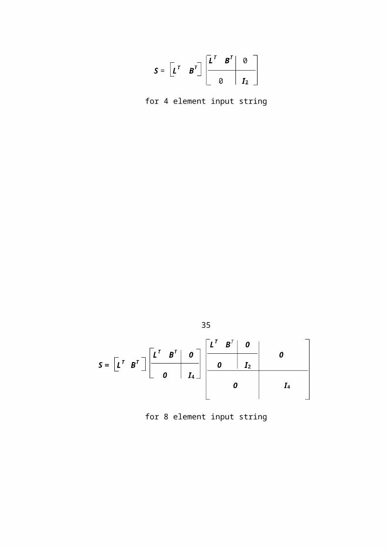
To compute the HL1 band, a low-pass filter operation is applied to the 8×4 matrix

from the above row transformation:

The process is analogous to that for HH1, except the filter takes averages of pixels

rather than differences.

Computing the other two bands is done in a similar fashion. First, a low-pass filter is

applied to the rows of the original pixel matrix:

76

Then, to compute LH1, a high-pass operation is done on the columns of the above 8×4

matrix:

The last of the four bands, LL1, is computed by applying a low-pass filter on the col-

umns of the above 8×4 matrix as follows:

The three bands HH1, HL1, and LH1 are left as they are. To obtain the second level of

decomposition, the process is now repeated on the LL1 band.

77A high-pass filter operates on the rows of the LL1 matrix:

A high-pass filter operates on the columns of the resulting 4×2 matrix to obtain HH2:

A low-pass filter operates on the same matrix to obtain HL2:

Now a low-pass filter is applied to the rows of the LL1 matrix:

A high-pass filter operating on this 4×2 matrix produces LH2:

A low-pass filter on the same matrix produces LL2:

78

To find the wavelet coefficients at the last level, filtering is done on LL2. First, a

high-pass filter operation on the rows:

Then a high-pass on the columns to yield HH3:

Now a low-pass on the columns to yield HL3:

For the other two bands, a low-pass operation is done on the rows of LL2:

Then, a high-pass operation is done on the columns of this matrix to yield LH3:

Finally, a low-pass filter is applied to the same vector to yield LL3, which is the over-

all average of the original image:

79

Combining all of the matrices resulting from the above computations results in the

following matrix shown in Figure 47:

Figure 47. Wavelet transform of pixel array representing the image in Figure 46

This matrix represents the image in terms of wavelet coefficients. This is a lossless

representation since all of the original pixel values can be easily recovered by ap-

plying inverse wavelet transformations. The example done here used the simple Haar

wavelets. In practice, Daubechies wavelets are used on images. The Haar wavelet

was used here for demonstration purposes.

5.2. Zero-Tree Structure

Now that the wavelet transform of images has been demonstrated, it is time to discuss

the compression algorithm.

The fundamental idea of the compression algorithm is keeping track of the significant

coefficients. These coefficients carry the most information of the image and they will

be what comprises the compressed image. However, not only is it important to keep

track of the coefficients themselves, but equally important, to keep track of the pos-

80

itions of those coefficients. Many of the coefficients will likely not be in the com-

pressed version of the image, and the locations of the coefficients that are left will

consequently be lost unless there is a method for keeping track of them.

To determine if a coefficient is significant, the coefficient is compared to a given

threshold. If the magnitude of the coefficient is greater than the threshold, then it is

significant. In other words, if it is greater than the threshold or less than the negative

of the threshold, it is considered significant. Insignificant coefficients, then, are those

whose magnitude is less than the threshold. This means that they are close to zero re-

lative to the threshold. Close to zero is considered zero.

In keeping track of positions of coefficients, the compression algorithm actually keeps

track of the locations of the insignificant coefficients rather than the significant ones.

The idea behind the algorithm is that if a coefficient is insignificant, then all coeffi-

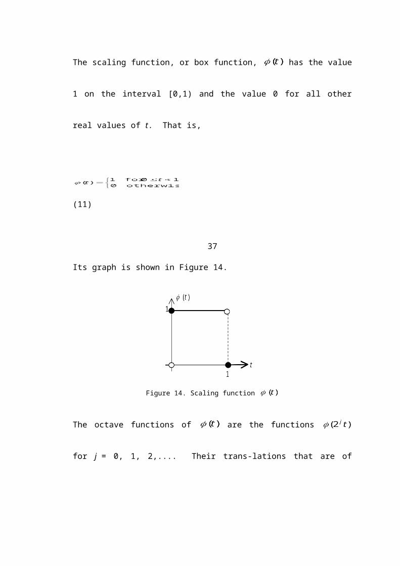
cients at the same orientation at finer levels are also likely to be insignificant [23].

This makes sense intuitively. Coarser levels are what represent most of the image, the

finer levels are simply fine details. Certainly, if a coefficient has no significance at a

coarse level, it likely does not have significance in a lower level since that level is

merely fine details. The structure relating positions of coefficients at various levels is

given in Figure 48. This is referred to as the zero-tree structure of the coefficients.

The term zero-tree will be explained shortly.

81

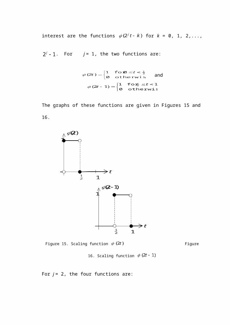
Figure 48. Zero-tree structure (Taken from [23])

There is a well-defined relationship between parent and child coefficients in the tree

structure. The coefficient in the LLK position (where K is the highest level) has three

children, one in each of the HLK, LHK, and HHK positions. The children of this coeffi-

cient are in the same level as the coefficient itself. Coefficients in the HL 1, LH1, and

HH1 bands do not have any children since they are at the finest level of detail. If the

coefficient is not in any of the LLK, HL1, LH1, or HH1 positions, then it has four child-

ren, which are in either the HLK-1, LHK-1, or HHK-1 band and at the same corresponding

position as their parent. This is evident in Figure 48 above. For example, the coeffi-

cient shown in the HL3 band spawns four children which are a block of four in the

HL2 band, and this block of four is oriented in the same position as the parent. Each

of these four coefficients have four more children of their own to result in a block of

16 in the HL1 band at the same orientation.

82

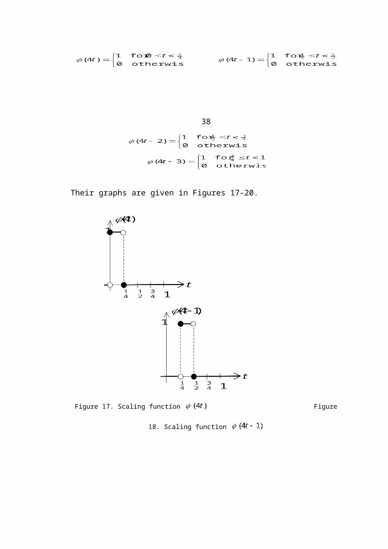
As a concrete example, consider the wavelet transformed matrix which is shown in

Figure 47. The tree structure for the coefficient in HH3, which is 8, is given in Figure

49. It has four children, -5, -6, -6, and 15 which make up the HH2 band. In turn, each

Figure 49. Zero-tree structure for HH3 band in Figure 47

of these children has four children of their own, each making up a block of four in the

HH1 band, in the same corresponding position as their parent. This is what makes up

the zero-tree structure of a coefficient. A coefficient is part of a zero-tree if it and all

of its descendants are zero with respect to the threshold. A coefficient is a zero-tree

root if all of its descendants are zero and that coefficient is not part of a zero-tree at a

coarser level.

There is a definite relationship between the array index of a coefficient and the array

indices of its children. If a coefficient has row and column indices (i, j), then the in-

dices of its children are:

Table 4. Indexing scheme for coefficients (Taken from [27])

This assumes that the array indices start at 1 and not at 0. In the concrete example

above, the indices of the coefficient 8 are (2, 2). Using the above indexing scheme,

the indices of the children are (3, 3), (3, 4), (4, 3), (4, 4) for –5, –6, –6, and 15 respec-

tively. The zero-tree structure and indexing scheme allow for the compression algor-

83

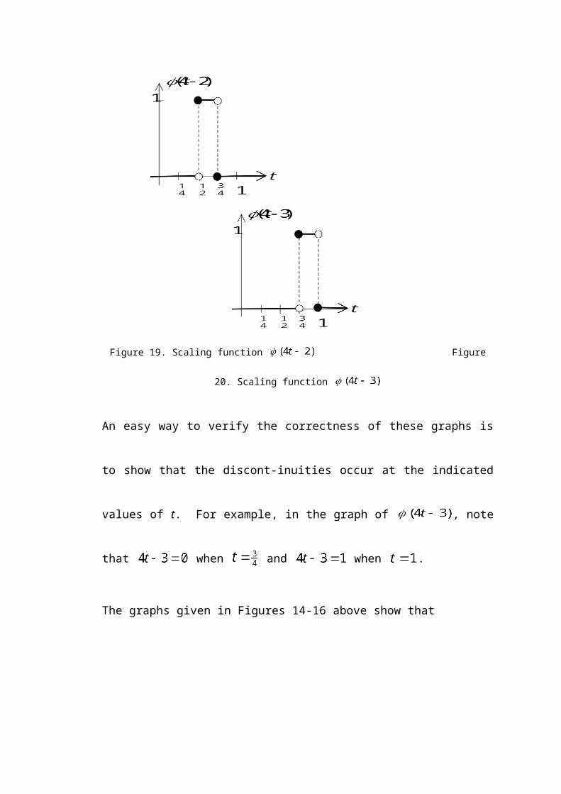
ithm to be more efficient. If a coefficient is a zero-tree root, its children and their pos-

itions do not need to be encoded. The children are assumed to have a value of zero

and their positions in the array are easily determined by the above indexing scheme.

5.3. Idea of the Image Compression Algorithm

The compression algorithm that is used in the JPEG2000 standard is the Embedded

Zero-tree Wavelet encoder, or EZW, which was introduced in 1993 by Shapiro [15].

Embedded means the same as progressive, where each pass through the algorithm

produces more refined, and thus more accurate versions of the image. The zero-tree

structure described above is used to determine significant and insignificant coeffi-

cients and their children. The word wavelet appears in the name since the algorithm

works with the wavelet transform of the image.

The EZW encoder scans the array of wavelet coefficients multiple times until the des-

ired level of detail or desired bit rate is achieved. During the scanning process, the

encoder determines the significant coefficients and the insignificant coefficients along

with their zero-trees by comparing the coefficients to a threshold. The threshold de-

creases with each pass through the wavelet transformed image, resulting in extracting

more detail from the image. The scan order that is used is illustrated in Figure 50.

Using this scan order guarantees that a coefficient will be scanned before any of its

descendants. This ordering is necessary in order to ensure that the zero-trees are

constructed properly.

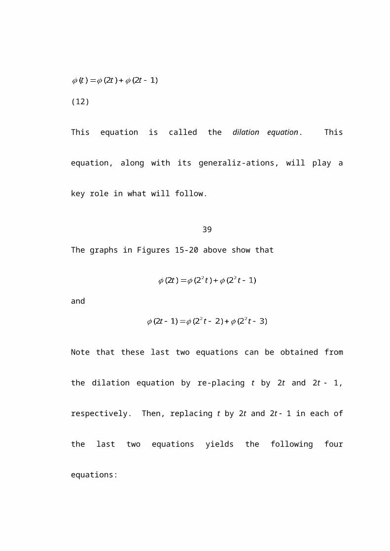
84

Figure 50. Scan order used in the EZW algorithm (Taken from [23])

The initial threshold is set to

(30)

where xmax is the largest coefficient in the wavelet transform matrix. The algorithm

consists of two passes, the dominant pass and the subordinate pass. These two passes

are described below.

In the dominant pass, the coefficient matrix is scanned to determine whether coeffi-

cients are significant or insignificant with respect to the current threshold. The ab-

solute values of significant coefficients are known to lie in the interval [T0, 2T0] and

the reconstructed value for the coefficient is 3T0/2. Coefficients cannot exceed 2T0

85

since those coefficients would have been found to be significant in the previous pass.

This is because the threshold is a power of 2 and it is divided by 2 before each suc-

cessive pass. The reconstructed value of the coefficient is simply the center of this in-

terval. The algorithm also notes whether a significant coefficient is positive or neg-

ative. For each insignificant coefficient that is scanned, it must be determined whet-

her it is the root of a zero-tree or just an isolated zero. The coefficients that are de-

duced to be zero based on a zero-tree root are not coded. A dominant list contains all

coefficients that were not significant on a previous pass. At the end of the dominant

pass, the significant coefficients that were found are moved to a subordinate list.

These coefficients will not be coded during subsequent dominant passes. The posi-

tions of these coefficients are set to zero in the wavelet transform array in order to

allow for the possibility that more zero-tree roots will be found in future passes.

After the dominant pass, the algorithm proceeds to the subordinate pass. This is also

known as the refinement pass. The encoder goes through the subordinate list and re-

fines the reconstructed values of these coefficients, which are all of the coefficients

that were found to be significant thus far. The interval [T0, 2T0] is divided into two

in-tervals of equal length, and they are (T0, 3T0/2) and (3T0/2, 2T0). The encoder

outputs a 1 if the coefficient lies in the upper interval of the two new intervals, and a 0

if it lies in the lower interval. The reconstructed value is now the center of the new

inter-val that the coefficient lies in.

After the subordinate pass, the threshold is divided by 2 for the next pass. The dom-

inant and subordinate passes are repeated until the threshold is less than 1 or the des-

ired level of detail or bit rate is achieved.

865.4. Bit Plane Coding

The EZW algorithm actually represents the coefficients as an arrangement of bit

planes. The bits of the coefficients are arranged so that the most significant bit is sent

first, that is, it appears in the lowest bit plane. The coefficient values, and therefore

the image, can be refined by adding more bits; each one is less significant than the

previous. The refinement process can be stopped at any time. This refinement pro-

cess is analogous to adding more and more digits to numbers such as π [24]. Adding

more digits increases the accuracy. The bit stream is embedded, that is, progressive,

where more and more detail is added with each bit.

During the first dominant pass, the most significant bit of the binary representation of

a wavelet coefficient is established. During the subordinate pass that follows, the next

most significant bit is determined. This bit plane representation is the reason why the

thresholds are powers of 2; it allows for the binary representation of a coefficient.

The encoding algorithm therefore extracts the binary representation of the wavelet co-

efficients of the image. Several bit planes are constructed, and the process is likened

to overlaying ever progressive versions of the image on top of one another, increasing

the amount of detail each time.

5.5. EZW Algorithm

Based on the discussion of the above sections, the EZW algorithm [23] is now given.

1. Initialization-Place all wavelet coefficients on the dominant list

-Set the initial threshold to

2. Dominant Pass-Scan coefficients on the dominant list using threshold T0 and the scan ordering scheme. Assign a coefficient one of the four symbols:

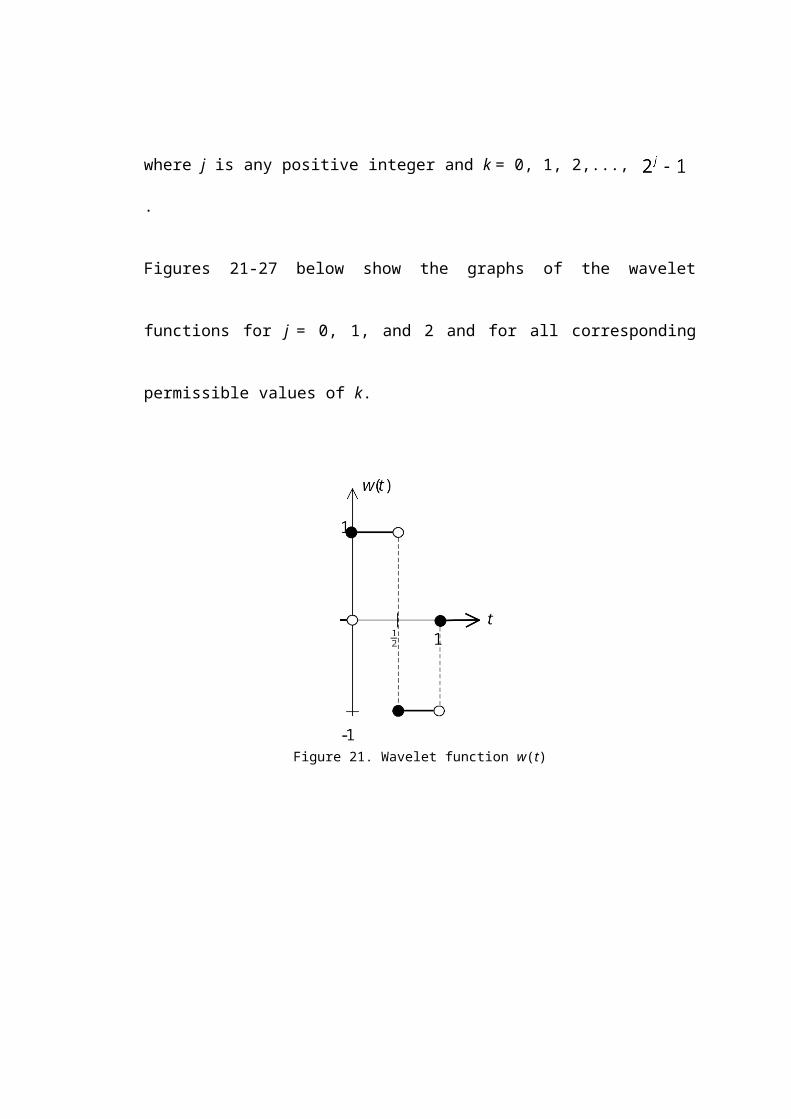
87-P (significant and positive)-N (significant and negative)-Z (isolated zero, coefficient is insignificant and one or more descendants is significant)-R (zero-tree root, coefficient and all descendants are insignificant)

-A coefficient that is a descendant of a coefficient coded as R is not coded-Move significant coefficients to subordinate list-Set values of significant coefficients to 0 in original wavelet transform matrix-Encode the symbol sequence

3. Subordinate Pass-Go through each coefficient on the subordinate list:

-Output 1 if coefficient is in upper half of interval [T0, 2T0]-Output 0 if coefficient is in lower half of interval [T0, 2T0]

4. Loop-Divide threshold by 2-Repeat 2-4 until desired level of detail or bit rate or until threshold is less

than 1

5.6. EZW Example

In this section, a concrete example will be shown to help explain how the EZW algor-

ithm works. Consider the example given in section 5.1 and the resulting wavelet

transform matrix given in Figure 47, which is repeated here.

First, the initial threshold is set. Since the largest coefficient in the matrix is 170, the

threshold is .

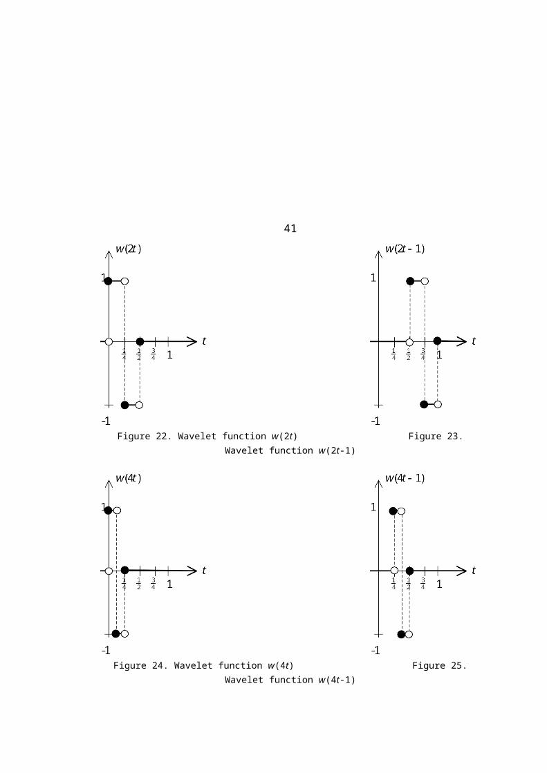
88In the first dominant pass, the threshold 128 is used along with the scan ordering

shown in Figure 50. The first coefficient scanned is 170. Since it is above threshold,

it is significant. It is also positive, which results in the symbol P being coded. The in-

terval of consideration is (128, 256) and the reconstructed value of this coefficient is

the center, which is 192. The next coefficient in the scan order is –68, which is insig-

nificant. Since this coefficient and all of its children, that is, all coefficients of the

HL2 and HL1 bands, are insignificant, this coefficient is a zero-tree root. The symbol

R is coded and all of its children need not be considered for the rest of the scanning

process of this iteration. This is shown below.

The next coefficient that is scanned is 7. Similar to –68, all of 7’s children are below

threshold, and so these children need not be considered either, and this coefficient is a

zero-tree root.

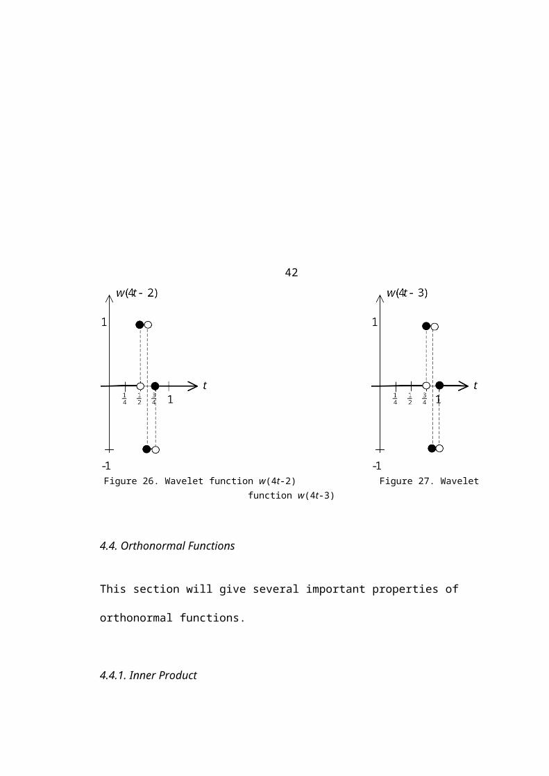
89The fourth coefficient scanned is 8. This is an insignificant coefficient and is also

coded as an R since all of its children are insignificant.

At this point, as the above matrix shows, there is nothing left to scan since the remain-

ing coefficients are deduced to be 0 as a result of having a parent as a zero-tree root.

The dominant pass stops here. The results are summarized in Table 5 below.

Table 5. First dominant pass of EZW example

The reconstructed value of the insignificant coefficients are defined to be 0, since they

are below threshold. The binary representation of the reconstructed value for 170 is

given and will be explained shortly. The entry in the matrix for 170 is replaced with a

0 for future passes.

After the dominant pass comes the subordinate pass. There is only one coefficient on

the subordinate list, 170, which is the significant coefficient found in the dominant

pass. In this pass, its reconstruction value is refined. The interval (128, 256) is divid-

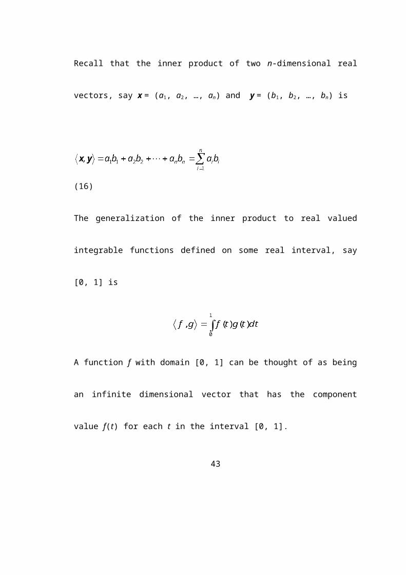
ed into two equal intervals to allow for more precision in the reconstruction. The two

resulting intervals are (128, 192) and (192, 256). The coefficient 170 is in the lower

90

interval so the output is 0. The reconstructed value is the center of this interval which

is 160. This value is much closer to 170 than 192 is. The binary representation for

160 is 10100000. The binary representation of 160 was derived from that of 192 by

keeping the first 1, changing the second bit to 0 (the output value determined by the

interval), and by sliding the second 1 in 192 to the right by one bit.

The wavelet coefficient array after the first pass is

If the image were to be reconstructed at this point, the pixel array would be

and the corresponding image is given in Figure 51. Since there is only one value in

91

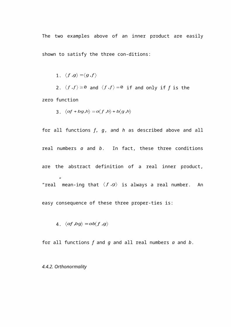
Figure 51. Reconstruction after one iteration of EZW

the coefficient array, the reconstructed image is made up of just that one value. The

reconstruction at this point is essentially the overall average of the original pixels.

This ends the first iteration of the EZW algorithm. Now the threshold is divided by 2

to become 64, and the dominant and subordinate passes are repeated.

The results from the second dominant pass are given in Table 6.

Table 6. Second dominant pass of EZW example

The first coefficient in the matrix is skipped over since it was already encoded in the

first dominant pass. One significant coefficient is found in the second pass, and it is

negative. However, the reconstructed values are only the magnitudes. The sign does

not need to be stored since the symbol N determines the sign of the coefficient. For

92

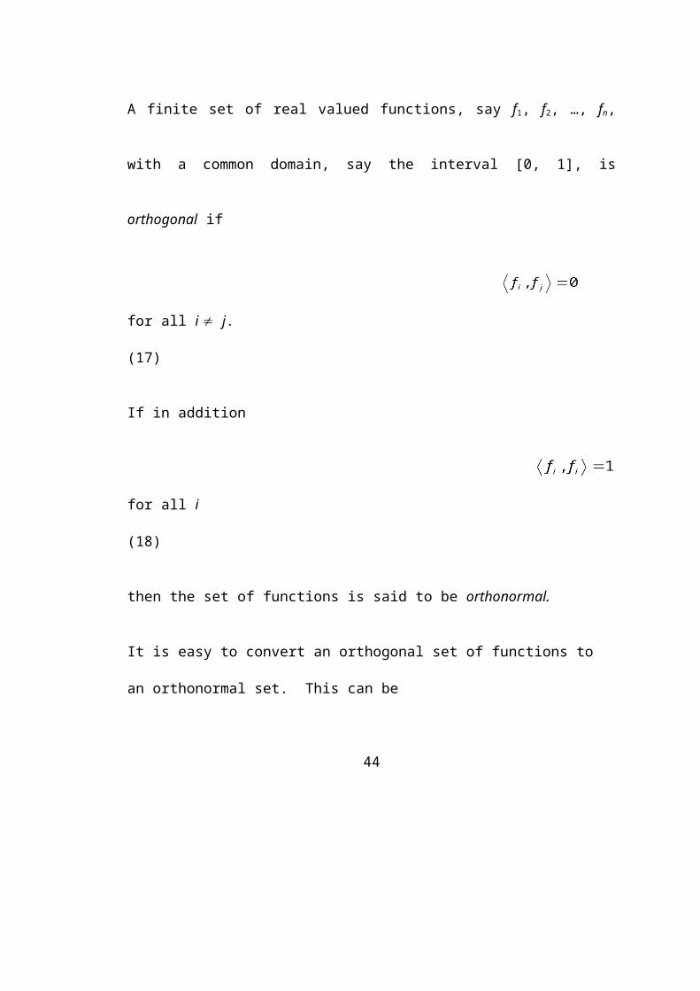
this pass, the scanning is taken one level lower into the HL2 band, since these are the

children of a significant coefficient. In the first pass, the significant coefficient (170)

did not have any children. Another point to notice is that the binary representation of

the reconstruction of –68 has one less bit than that of 170. This results from the thres-

hold being divided by 2. At the end of this pass, 68 is added to the subordinate list

and its position in the coefficient array is set to 0.

The subordinate pass will again refine the reconstructed values by adding the next

most significant bit to the binary representation. The interval of consideration in this

step is (64, 128). As before, this interval is divided into two intervals, (64, 96) and

(96, 128). In addition, each of the two intervals from the first subordinate pass are di-

vided into two to yield four more intervals: (128, 160) and (160, 192) (from (128,

192)) and (192, 224) and (224, 256) (from (192, 256)). Each pair of intervals deter-

mines the upper and lower intervals for the coefficients and thus whether the output is

1 or 0. The coefficient 170 was in the interval (128, 192) from before and now it is in

the associated upper interval (160, 192) so the output is 1 and the reconstructed value

is the center which is 176. The coefficient 68 lies in the lower interval of (64, 128),

which is (64, 96), so the output is 0 and the reconstructed value is the center which is

80. The results are given in Table 7 below.

Table 7. Second subordinate pass of EZW example

In the binary representation for 170, the first two bits stayed the same, the third was

replaced by the output 1, and the 1 that was in the third position is now in the fourth

position from the left. In the binary representation for 68, the first 1 was left as it is,

the second bit was replaced by output 0, and the 1 that was there now slides over one

into the third bit from the left. The reconstructed values have now been refined by

93

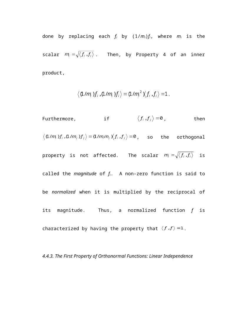
one more bit than before, hence adding another level in the bit plane representation.

The wavelet coefficient array after the second iteration is

The reconstructed pixel array is

and the corresponding image is given in Figure 52. Since there is now a difference

94

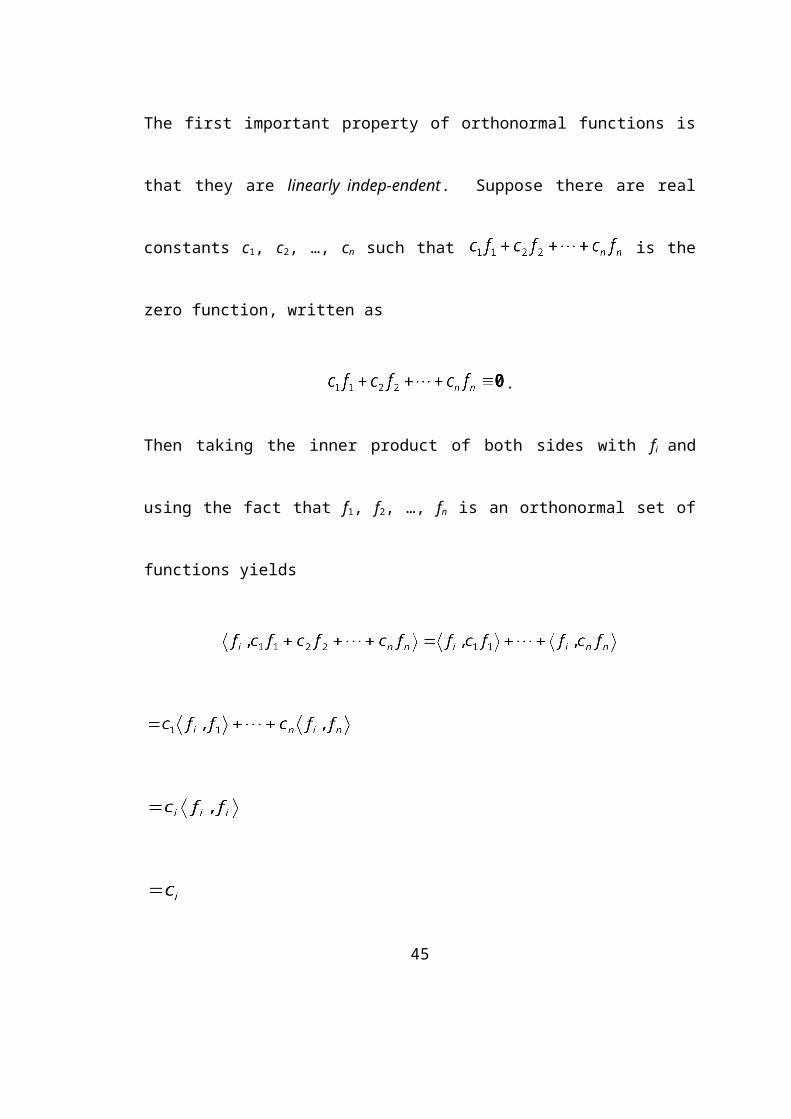
Figure 52. Reconstruction after two iterations of EZW

among the coefficients, the algorithm is able to make a distinction between dark (left

side of the image) and light (right side of the image).

The threshold is divided by 2 to become 32 and the third iteration of the algorithm

begins. The results of the third dominant pass are given in Table 8.

Table 8. Third dominant pass of EZW example

In this pass, the symbol Z is found for three of the scanned coefficients. These coeffi-

cients are located in the HL1 band, so they do not have any children. They cannot be

a root of a tree, so they are just considered isolated zeros. The last four coefficients in

the table needed to be scanned since they are the children of –53, which is a signi-

95

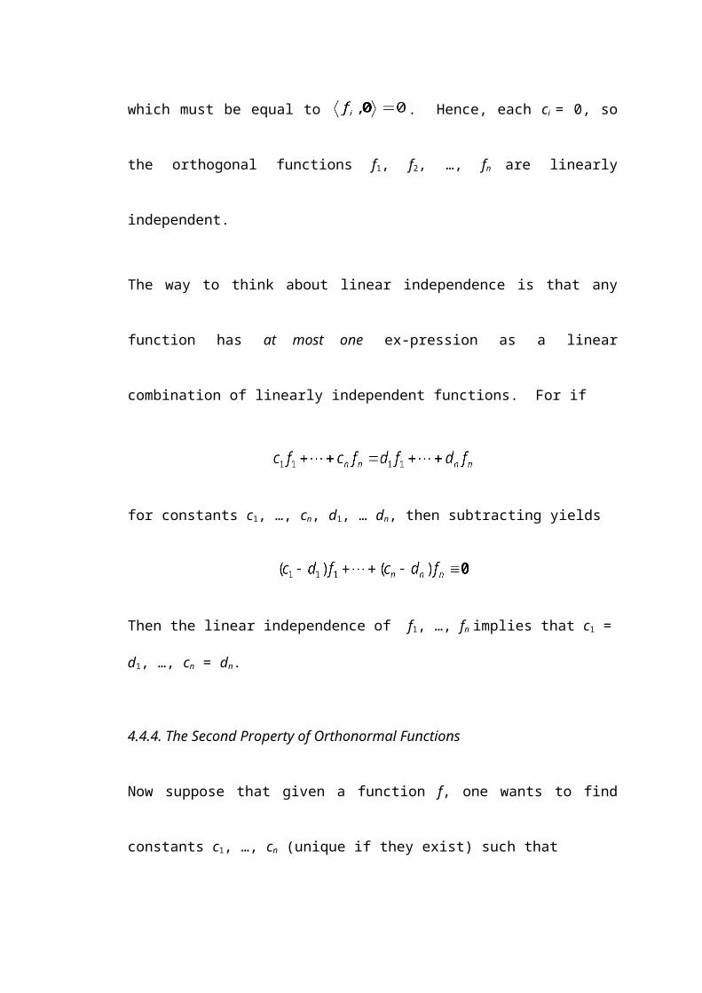
ficant coefficient in this pass. Upon scanning these four coefficients, another signi-

ficant coefficient is found, which is –36. Note that the binary representation of 48

again has one less bit than the previous pass because of the threshold being divided by

2.

The magnitudes of the two significant coefficients, 53 and 36 are appended to the sub-

ordinate list resulting in four elements on the list. The interval (32, 64) is divided into

two intervals (32, 48) and (48, 64) and all intervals from the previous subordinate pass

are also divided into two. The resulting pairs of intervals are shown in Table 9 and

the results of the third subordinate pass are given in Table 10.

Table 9. Intervals for third subordinate pass of EZW example

The first pair of intervals comes from the interval introduced in the third dominant

pass, the other pairs are derived from intervals of the previous iteration.

Table 10. Third subordinate pass of EZW example

As before, the reconstructed values are refined to be even closer to the actual coeffi-

cient values, and with each pass, one more significant bit is added to the binary repre-

sentation of these values. The fifth bit from the right is identical to the output bit in

this pass.

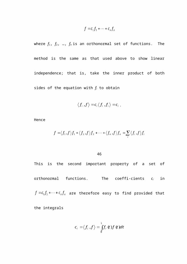
96The wavelet coefficient array after the third iteration is

The reconstructed pixel array is

and the corresponding image is given in Figure 53. As more non-zero coefficients are

Figure 53. Reconstruction after three iterations of EZW

97added to the wavelet coefficient array, the algorithm is able to make out more and

more details in the reconstruction of the image.

In the fourth iteration, the threshold becomes 16. Partial results of the dominant pass

are shown in Table 11. Only the results for the upper left quadrant are shown. The

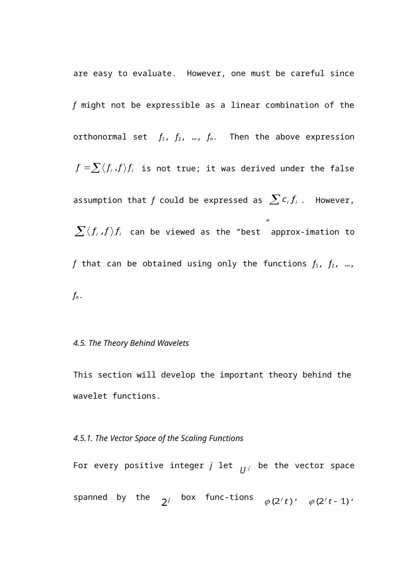
rest of the values are either significant (positive or negative), or they are (trivially)

isolated zeros.

Table 11. Partial fourth dominant pass of EZW example

There is one thing that happens here that did not in previous dominant passes. There

are isolated zeros found in the upper left quadrant, even though all of these coeffi-

cients have children at lower levels. The reason these coefficients cannot be zero-tree

roots is because at least one child is significant with respect to the current threshold.

For example, the coefficient 7 in LH3 has children –14, –9, 27 and 10 in LH2, of

which 27 is above threshold. The coefficient 8 in HH3 does not have any direct

children (coefficients of HH2) that are significant, but there is a subsequent child,

namely, 18 in HH1, that is above threshold. Thus, 8 is not a zero-tree root. A

coefficient cannot be a zero-tree root if any of its children are above threshold, which

includes children of children.

98

The results of the subordinate pass of the fourth iteration are shown in Table 12. Bin-

ary representations are only shown for the first four coefficients.

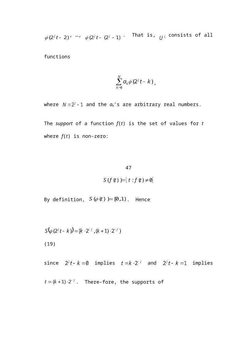
Table 12. Fourth subordinate pass of EZW example

The wavelet coefficient array at this stage is

The reconstructed pixel array is

99and the reconstructed image is given in Figure 54.

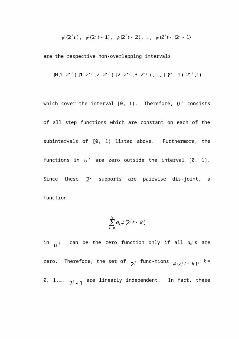
Figure 54. Reconstruction after four iterations of EZW

The algorithm can continue for three more iterations. After the seventh iteration, the

threshold is 1. Another dominant pass would be made, but at that point, there are no

significant coefficients that are left to be found; they were all found in a previous

pass. The remaining passes work in the same manner as the previous passes and will

not be demonstrated in this paper. However, Tables 13-15 show the results for the

first four coefficients of the remaining three subordinate passes. The output bits and

the binary representations will be of interest in a later section.

Table 13. Partial fifth subordinate pass of EZW example

The wavelet coefficient array after the fifth iteration is

100

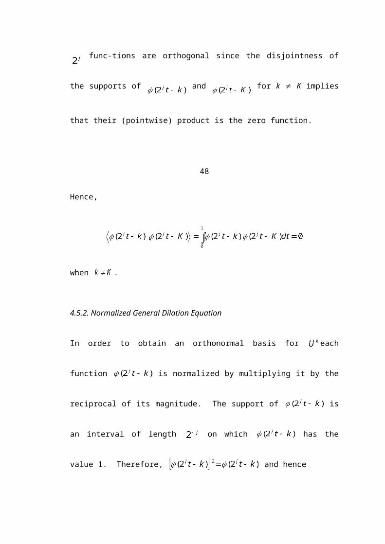
The reconstructed pixel array is

and the reconstructed image is given in Figure 55. Pixel values continue to be fine-

tuned.

Figure 55. Reconstruction after five iterations of EZW

101Partial results for the sixth iteration are given in Table 14.

Table 14. Partial sixth subordinate pass of EZW example

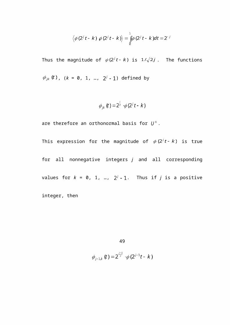
The wavelet coefficient array is

The reconstructed pixel array is

and the corresponding image is shown in Figure 56. At this point, only very fine

102

Figure 56. Reconstruction after six iterations of EZW

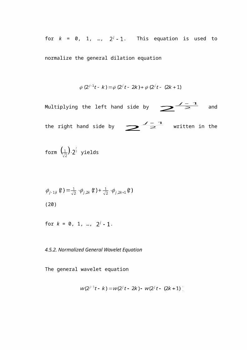
details are added to the reconstruction of the image.

Partial results for the seventh pass are shown in Table 15.

Table 15. Partial seventh subordinate pass of EZW example

In the binary representations of the last pass, the last bit is assigned to the output

value, and the 1 that kept sliding along the bit string is essentially pushed off of the

end of it. What is left is the binary representation of the original wavelet coefficients.

Iterating as far as possible produces perfect reconstruction of the coefficients. Of

course, it is likely that it would be desirable to stop the iterations sooner, so as to

result in more compression. When to stop is dependent on the desired level of detail

or the bit rate. Each iteration results in a progressive refinement of the image, by

adding a more de-tailed bit plane on top of the previous bit planes. Internet browsers

use this technique in downloading pages containing images. If the user can tell early

on that the image

or page is something that they do not want, they can abort the transmission in the mid-

103

dle of the process without having to wait for the final image to download.

Figure 57 shows the sequence of the images displayed above, in progressive order

from coarsest approximation to the full image.

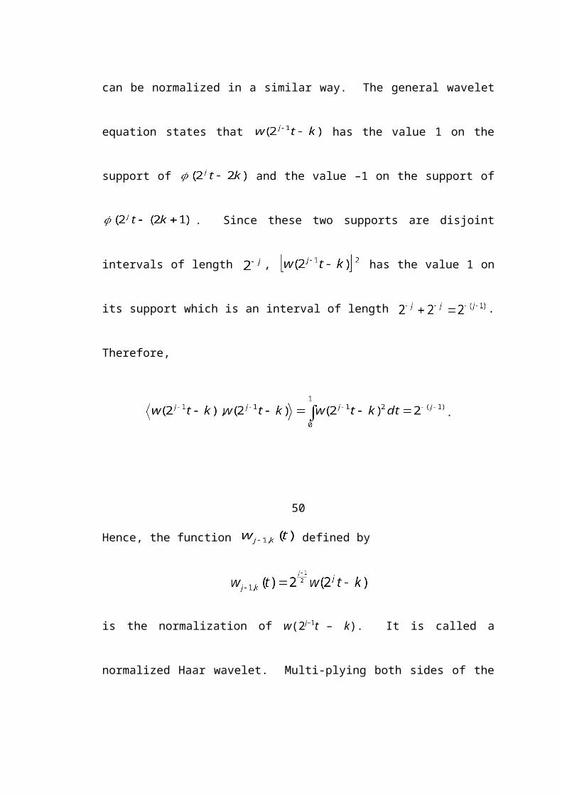
Figure 57. Progressive refinement of image given in Figure 46

The compressed version of the image is stored in an output file. The beginning of the

file contains some basic header information such as the wavelet transform type,

image size (number of rows), log2(threshold), and the number of bit planes. After this

information, the file contains the output from the dominant and subordinate passes of

each iteration of the EZW algorithm. From the dominant pass, the coefficient

symbols P, N, Z, or R are the output. Since there are only four possible symbols, each

of these can be stored by using two bits [27], so the combinations would be 00, 01,

10, and 11. The output from the subordinate passes consists of the 0’s and 1’s that

were output based on whether the coefficients were in lower or upper intervals. A

partial output file for the example given above is shown below in Figure 58.

104

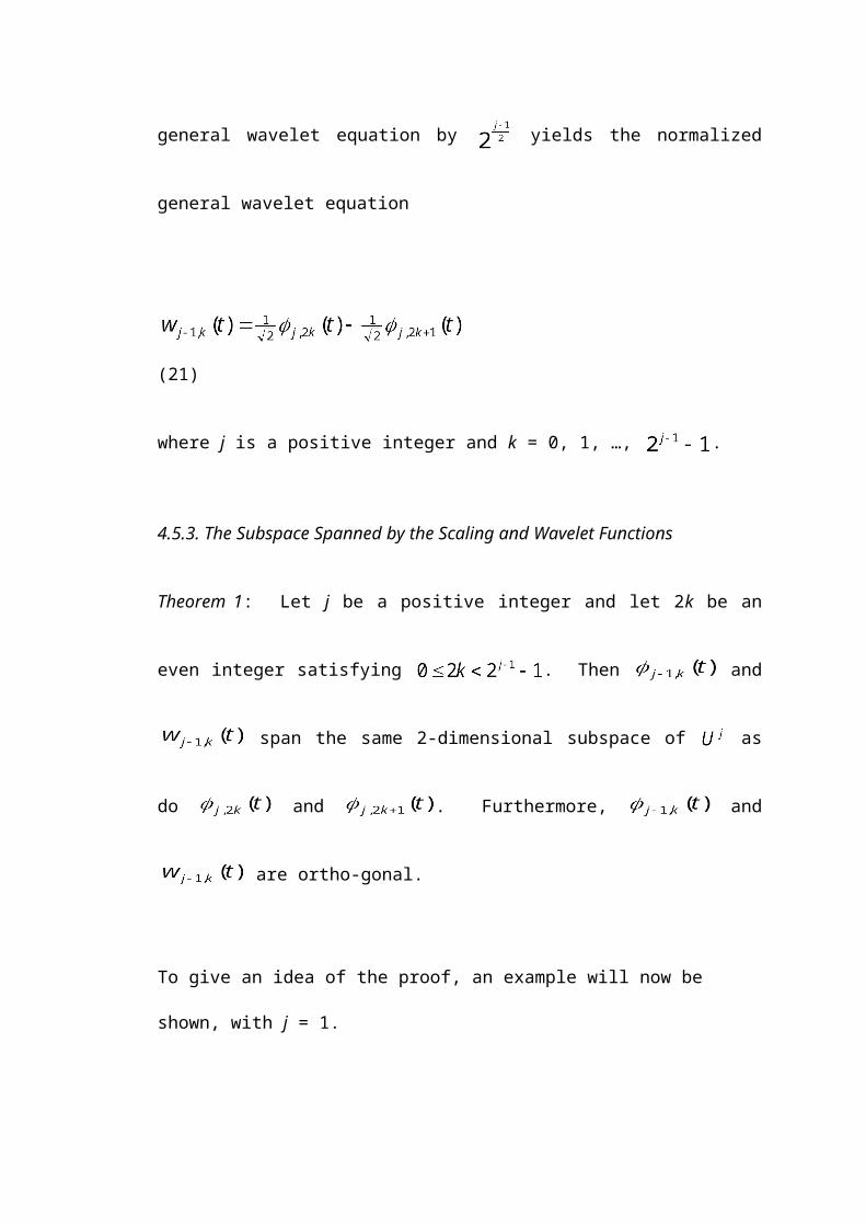
Figure 58. Partial output file for EZW example

As mentioned above, the symbols are actually coded using one of the binary sequen-

ces; they are shown as characters here for demonstration purposes.

5.7. Decoding the Image

For decoding an image, the bit planes for the coefficients are built up using the bits

from the compressed image file. First, the symbols are read into a symbol array,

which has the same dimensions as the wavelet transform matrix. The symbols are

read into the array in the same order as the scanning order shown in Figure 50. When

a zero-tree root symbol occurs, the children are expanded and filled with a different

symbol. The index relationship illustrated in Table 4 makes this process straight-

forward. Once the symbol array is constructed, the decoder uses the output corres-

ponding to the bits produced in subordinate passes to reconstruct the wavelet coeffi-

cients. The first iteration of the process starts with the initial threshold read in from

the data file and this threshold is divided by 2 for each subsequent iteration. The de-

105

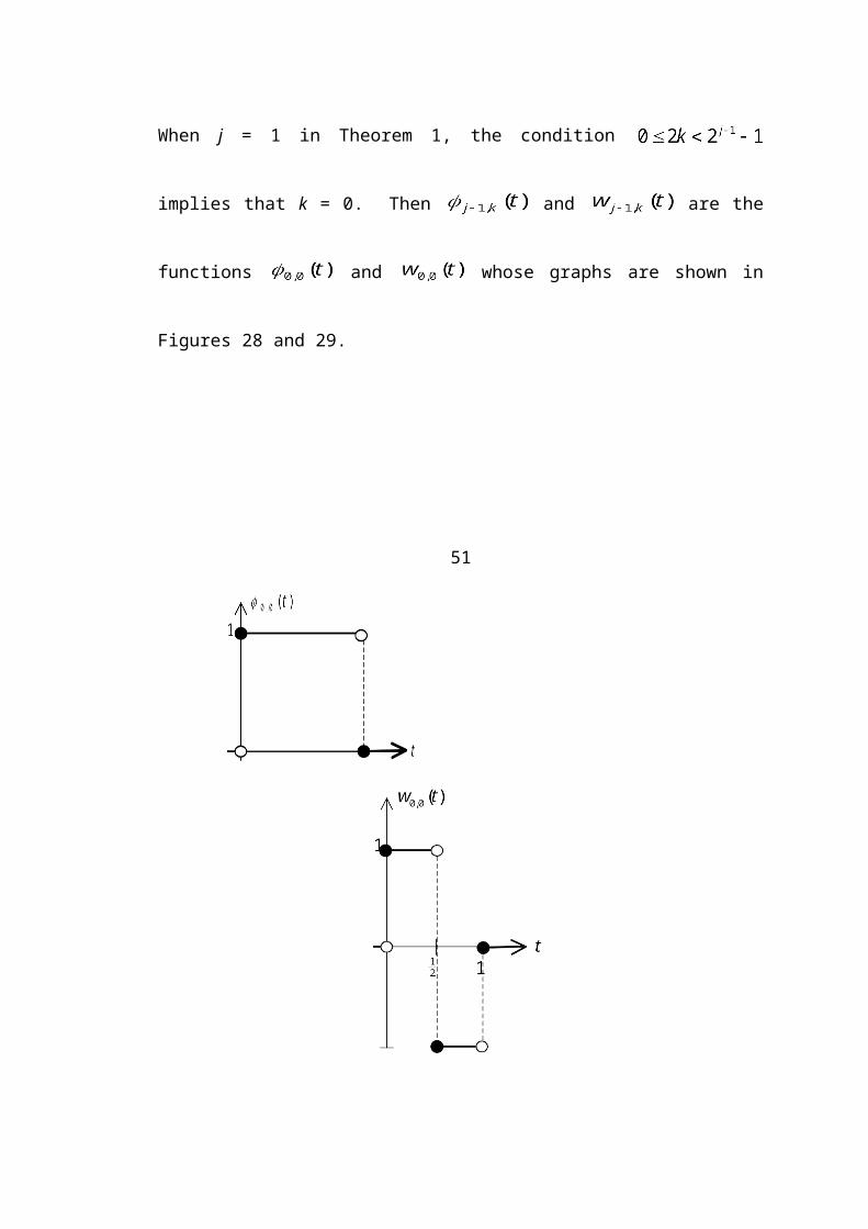
coder is iterated until the threshold is less than 1 or the number of iterations is equal to

the number of bit planes. The decoding process for the example shown in Section 5.6

will be demonstrated here.

For the first iteration, the threshold T is 128. The reconstructed value starts as 3T/2.

This corresponds to the first dominant pass in the EZW process. The threshold is then

decreased to 64.

The reconstruction value of the first significant coefficient is refined at this stage,

which corresponds to the first subordinate pass. The decoder examines the output

value from the file for each significant coefficient. If it is a 1, then T/2 is added to the

magnitude of the reconstructed value, and if it is a 0, then T/2 is subtracted. There is

a special case when T = 1. In this case, if the output is 0, then 1 is subtracted, if it is a

1, no action is taken. This process builds up the reconstructed values one bit at a time,

just as in the dominant and subordinate passes of EZW.

In this example then, 0 appeared in the output file for the first subordinate pass, so

T/2 = 32 is subtracted from 192 to yield 160, which is the same reconstruction value

as in the first subordinate pass of EZW. The symbol array is filled again at this point,

this time with the values from the second dominant pass. The P’s and N’s that were

already there are left alone. During this iteration, another significant coefficient is en-

countered, so its place in the array is filled with –96 since 3T/2 = 96 and the coeffi-

cient is negative. This corresponds to the second dominant pass.

The threshold is decreased to 32 and another iteration begins. The two coefficient

values are refined by one more bit. For the first one, the output from the file is a 1, so

T/2 is added to the reconstruction, which means 160 becomes 176. For the second co-

efficient, the output is a 0, so T/2 is subtracted from the magnitude of –96, which re-

sults in –80. Negative coefficients work in the opposite way as positive coefficients.

106

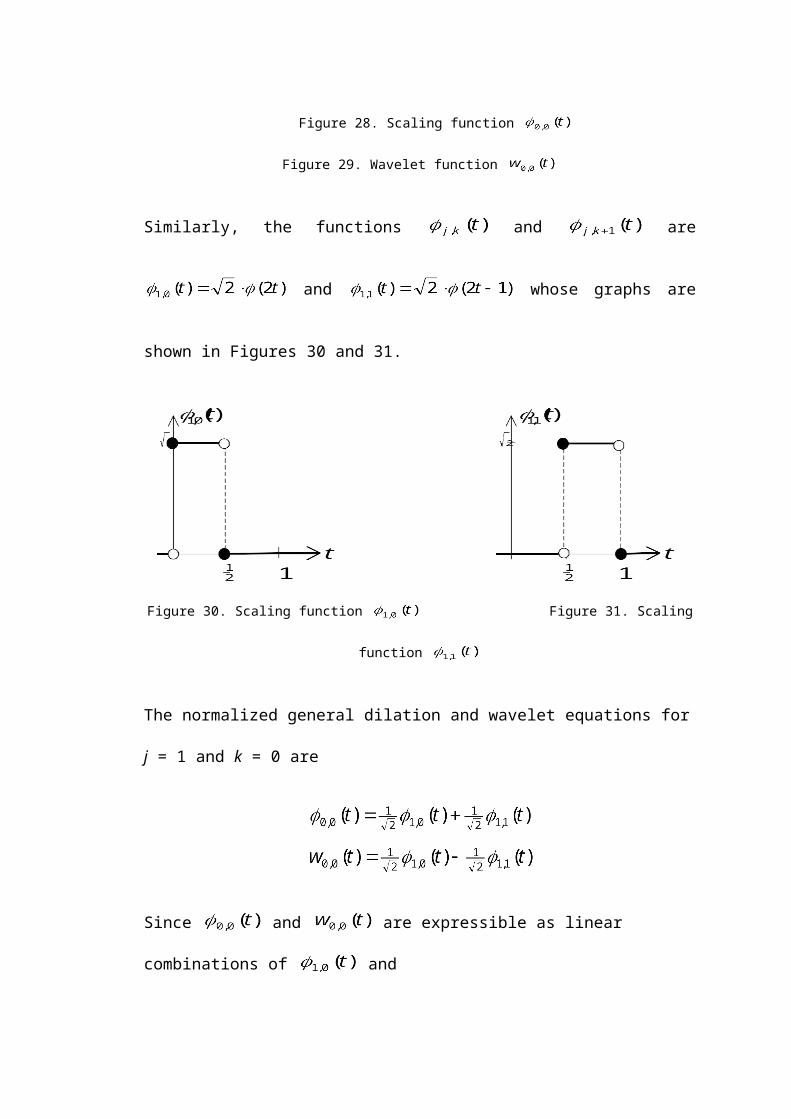
The main point is that T/2 is added to or subtracted from the magnitude of the recon-

struction. Refining these two coefficients produces values exactly as those from the

second subordinate pass of EZW. Two new significant coefficients are found and the

values –48 are added in their places in the array since 3T/2 = 48 and both coefficients

are negative.

Figure 59 shows the symbol array for this iteration. It contains the symbols read from

the dominant passes of the output file. A child of a zero-tree root is denoted by a “”.

Figure 59. Symbol array of third iteration of decoding process

This process continues, decreasing the threshold each time and refining the significant

values in the array one bit at a time. The entire reconstruction process for the first

four significant coefficients is shown in Figure 60. The reconstructed wavelet array is

actually a two dimensional matrix as shown before. The coefficients are shown here

in a linear array for simplicity of this example.

107

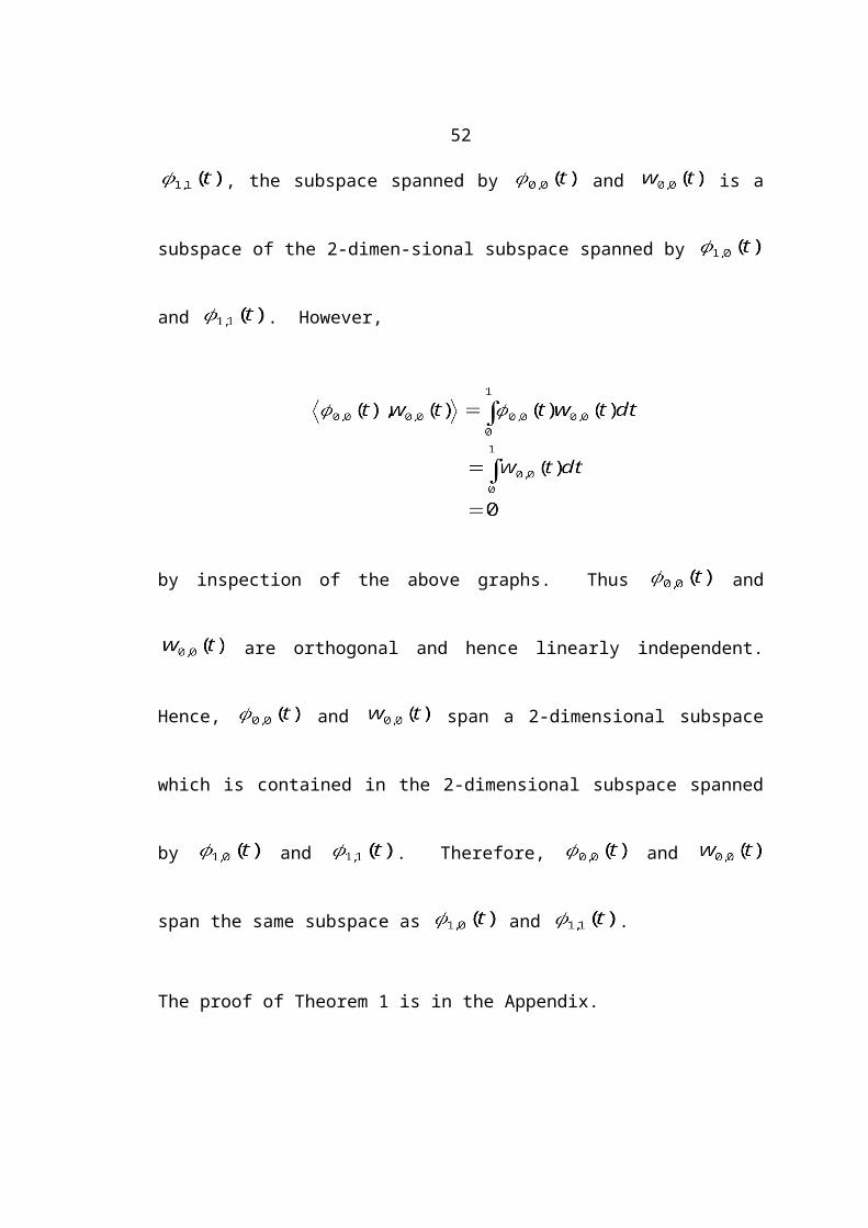
Figure 60. Reconstruction of wavelet coefficients in decoding process

The reconstructed values for each iteration correspond to the reconstructions calcu-

lated during the subordinate passes of the EZW algorithm. The last set of reconstruct-

ed values contains the actual values of the original wavelet coefficients. This process

can be stopped at any time, depending on the desired level of detail. To recover the

pixel values of the image, the inverse wavelet transform is applied to the reconstruct-

ed coefficient matrix.

5.8. Inverse Wavelet Transform

This section will demonstrate how to go from the wavelet coefficient array back to the

pixel array. The operation for doing this is an inverse wavelet transform. The ex-

ample shown here will essentially work in the backwards direction of the example

shown in Section 5.1. With each operation, the intermediate averages and differences

will be recovered and eventually the entire original pixel array will result.

Consider the wavelet coefficient matrix:

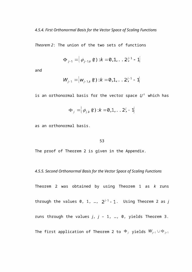
108

The first operation will be on the 2×2 upper left corner. The 2×2 filter matrix assoc-

iated with the forward operation is

where the top row indicates the low-pass operation and the bottom row indicates the

high-pass operation.

The inverse of this matrix ends up being the transpose, ignoring the factor:

which happens to be the same matrix in this case. This can be verified by checking

that

This matrix is the inverse operator on the columns of the upper left corner of the

coefficient matrix. Multiplying the matrices produces

109

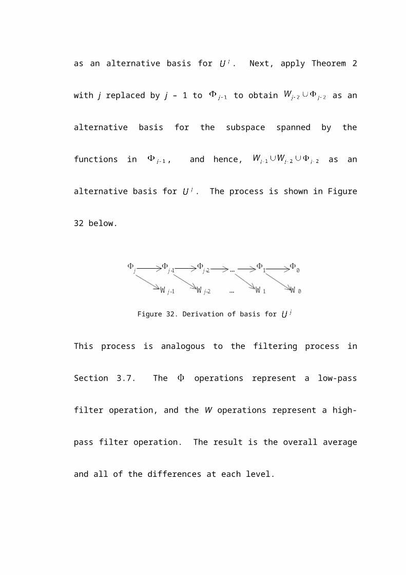
Note that the columns of the resulting matrix are the intermediate vectors from per-

forming low-pass and high-pass operations on the matrix LL2.

Now the inverse transform must be done on the rows of this new matrix. The trans-

pose is calculated and multiplied on the right side of the above matrix. The transpose

of the filter matrix happens to be the same in the 2×2 case.

The resulting matrix is LL2 from the operation on the original pixel array. Note that

in LL2, the bottom-left entry was 88. The deviation of values in this operation is due

to round-off error that was introduced in producing convenient integer coefficients.

The next stage will operate on this new matrix along with the NE, SW, and SE cor-

ners of the 4×4 upper-left corner of the wavelet coefficient array. The inverse

operation on the columns is

The resulting matrix contains two 4×2 matrices (except for round-off error) that were

produced by performing low-pass and high-pass operations on the rows of LL1. In the

matrix above that is multiplied by the filter, the upper left corner contains LL2, the

other corners are HL2, LH2, and HH2.

Now the inverse row transform is performed on the above result matrix:

110

The matrix that results from this operation is LL1. Again, the entries deviate slightly

because of round-off error.

In the last stage, the columns of the above resulting matrix, along with HL1, LH1, and

HH1 are multiplied by the inverse filter operator:

Now the inverse row operation is done on the resulting matrix:

111

The resulting matrix is the original pixel array, with some values off slightly due to

round-off error. This does not create a problem since the intent is only to show the in-

verse process, not to obtain precise values. There were also a few places in the calcu-

lations where values went out of the 0-255 range. The values were adjusted to be the

appropriate endpoint. The operations performed above are essentially the reverse of

the forward process presented in Section 5.1. The operations here “undo” what was

done there in order to recover the original pixel matrix.

The inverse operations that were shown in this section used the Haar wavelet trans-

form. As before, the Daubechies wavelets are used in practice.

5.9. Extension of EZW

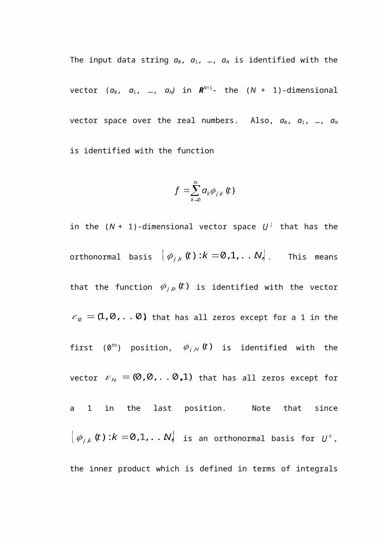
An enhancement of the EZW algorithm, Set Partitioning in Hierarchical Trees

112

(SPIHT), was introduced by Said and Pearlman in 1996 [14]. As explained in their

paper, the algorithm uses principals of partial ordering by magnitude, set partitioning

by significance of magnitudes with respect to a sequence of octavely decreasing thres-

holds, ordered bit-plane transmission, and self-similarity across scale in the image

wavelet transform. This algorithm produces a fully embedded image file by changing

the transmission priority and ordering coefficients differently than in EZW. What

fully embedded means is that a single file for an image can be truncated at any time

and the decoding gives a series of reconstructed images at lower rates.

The SPIHT method produces results that are superior to those of EZW, in terms of

image quality and compression rate. The algorithm exploits all of the following pro-

perties simultaneously: highest image quality, progressive transmission, fully em-

bedded coded file, simple algorithm, fast coding and decoding, completely adaptive

for different applications, exact bit rate coding, and error protection [16]. More de-

tails on the implementation of the SPIHT algorithm can be found in Said and

Pearlman's paper [14].

5.10. Demonstration Software

There is an interactive learning tool for image compression available on the Internet.

It allows a user to load an image and perform various compression algorithms, from

DCT to EZW on the image. It is available free from [8].

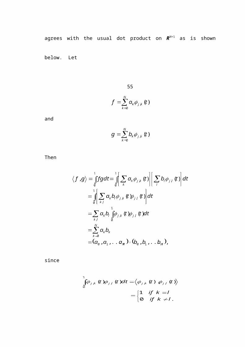
113

6. Performance of Wavelet Image Compression

This section will give a few results and briefly discuss the performance of different

wavelet image compression methods compared to one another and to earlier tech-

niques.

The graph in Figure 61 shows the performance of several different compression

schemes.

Figure 61. Comparison of compression algorithms (Taken from [13])

The measure for determining performance that is used is the PSNR, which is the peak

signal to noise ratio. This ratio represents how much useful information there is com-

pared to how much noise or errors that have been introduced. Image compression

was applied to the Lena image given in Chapter 2. The JPEG method is used as the

baseline. The zero-tree method is the EZW algorithm, and the other methods are pre-

vious wavelet techniques. At low compression rates, JPEG actually performs better

than the earlier wavelet methods. However, at higher compression rates (30+), the

114

performance of JPEG falls rapidly, while the other methods degrade gracefully. The

graph clearly shows that the zero-tree method performs far better than any of the other

methods, including the previous wavelet methods.

Figure 62 shows reconstruction of the Barbara image from performing compression

Figure 62. Barbara image using JPEG (left) and EZW (right) (Taken from [23])

using JPEG and EZW. A three level decomposition was used and the rate was 0.2

bits/pixel. The PSNR value for JPEG is 23.3 dB and for EZW it is 24.4 dB. There is

a noticable difference in the visual quality of the images as well. The JPEG image ap-

pears slightly more fuzzy whereas the EZW image is more smooth.

Figure 63 shows the results of compressing the Lena image using Daubechies D4

Figure 63. Lena reconstructed using 10% and 5% of the coefficients using D4 wavelets (Taken from [27])

115wavelet with 10% and 5% of the coefficients respectively. Certainly, the image using

only 5% of the coefficients is of considerably less quality than the one using 10%.

Figure 64 shows the original and reconstructed Winter image using D4 wavelets with

10% of the coefficients.

Figure 64. Winter original and reconstruction using 10% of the coefficients using D4 wavelets (Taken from [27])

The D4 method does not perform very well here and the main reason for this is that

the Winter image contains more high-frequency detail than the Lena image. This

result shows that a wavelet method does not perform equally on every image and

suggests that the best choice of wavelet method is image dependent.

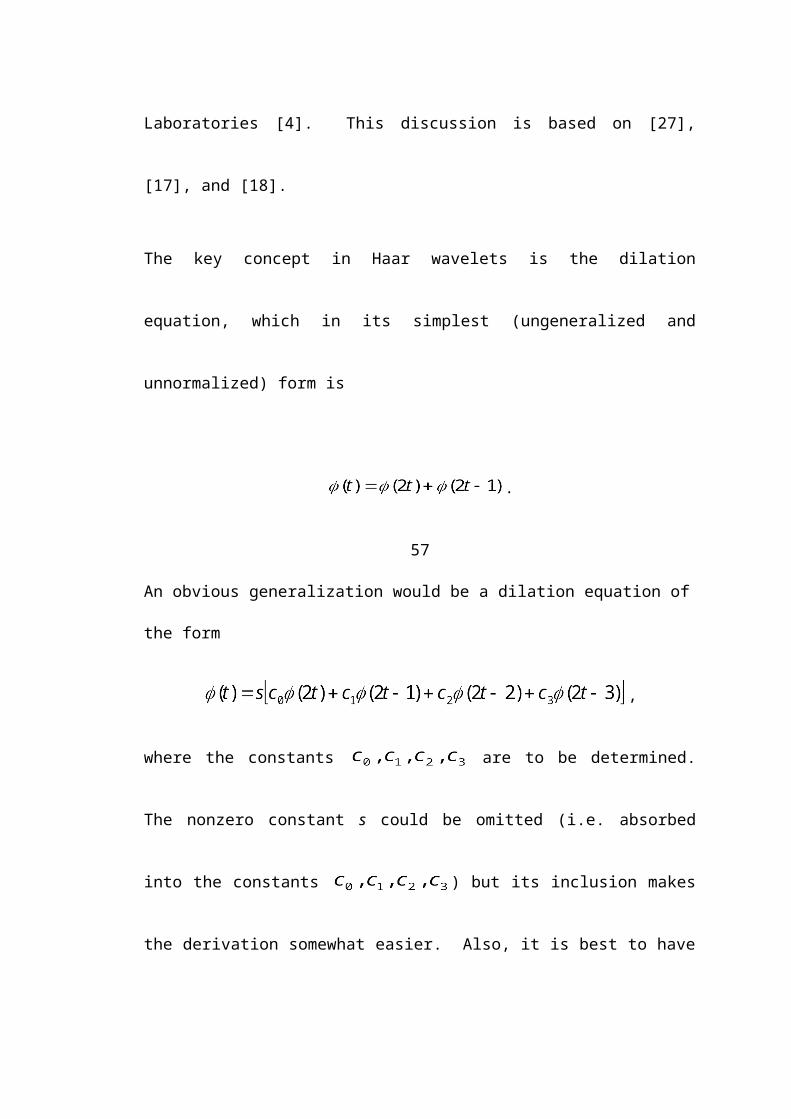
Tables 16 and 17 show the PSNR values for three wavelet techniques: Haar, D4 and

Table 16. Results of three wavelet methods on Lena image (Taken from [27])

116

Table 17. Results of three wavelet methods on Winter image (Taken from [27])

D6 on the Lena and Winter images. Figure 65 shows a graph of these data. The

Figure 65. Graph of results of Lena and Winter images for three wavelet methods (Taken from [27])

Daubechies wavelets definitely out-perform the Haar wavelet for the Lena image, but

for the Winter image, the three methods have nearly the same performance.

117

7. Applications of Wavelet Image Compression

This section will briefly discuss several real world applications of image compression

using wavelet techniques.

7.1. Medical Imaging

Aware, Inc [2] was the first commercial organization in the world to provide a wave-

let image compression algorithm for use in medical applications. Lossless compres-

sion can achieve ratios of 2:1 or 3:1. One feature is that multiple smaller blocks of the

image can be extracted and progressively decoded. An example showing the quality

of image reconstruction is shown in Figure 66. The first uses lossless compression

and the second uses lossy compression with a ratio of 20:1.

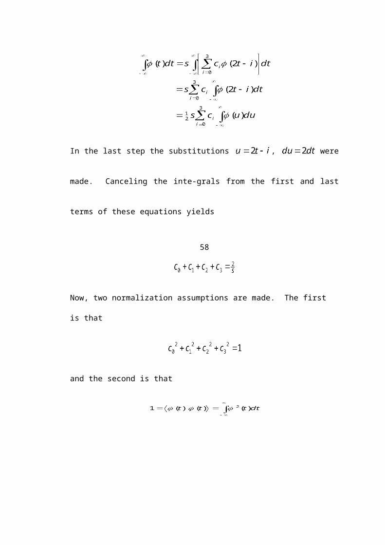
Figure 66. Medical image reconstructed from lossless and 20:1 lossy compression (Taken from [2])

Another feature is progressive display. The image file has a multi-layered format.

The resolution or image quality is refined as more image data is received. Figure 67

shows an example of how this is done.

One more important feature of medical image compression is the use of region of in-

terest encoding. In this method, important features are compressed so that higher qua-

lity is maintained, whereas the background features are allowed to be of lesser quality.

Thus, the image file can be compressed considerably without losing essential details.

118

Figure 67. Progressive refinement of medical image (Taken from [2])

7.2. FBI Fingerprinting

A single fingerprint card contains about 10MB of data. Since 1924, 200 million fin-

gerprints have been collected by the FBI, which totals approximately 2000 terabytes

of information occupying an acre of file cabinet space in the J. Edgar Hoover building

in Washington. On top of this, between 30,000 and 50,000 new fingerprint cards are

accumulated per day. The time to transmit one 10MB card at a rate of 7680 bits/sec is

almost 3 hours [3].

Obviously, all of these facts imply that effective image compression methods are es-

sential. Lossless methods can only accomplish a compression rate of 2:1, which does

not result in a significant difference. Therefore, lossy techniques must be used. How-

ever, a fingerprint image has very fine detail that must be preserved. In the finger-

print image given in Figure 68, the tiny white spots in the black ridges are sweat

pores,

which function as key identification features in a court case. Using the JPEG method

119

Figure 68. FBI fingerprint image showing fine details (Taken from [3])

at a compression ratio of 12.9:1 results in losing these very fine details in addition to

introducing the blocking effect in the reconstructed image. A wavelet technique,

known as WSQ (Wavelet/Scalar Quantization) used on the same image at the same

compression rate preserves the fine details much better than the JPEG method, and

also eliminates the blocking effect.

7.3. Computer 3D Graphics

Image compression can also be applied to 3D digital models [9]. There are several

ways to manipulate data for more efficient transmission and storage, although each

120

has its disadvantages. Information can be removed from the file, but this results in in-

formation that is lost and must be recreated at the receiving end. The geometry can be

altered to obtain an approximation of the figure, but this may result in the shape being

corrupted or deformed. The model could be sent in progressive stages, but this may

result in the transmission time being too long. It is important to find an optimal bal-

ance between the tradeoffs concerning geometry, attributes such as color or texture,

transmission speed, and processing or storage requirements.

Most 3D models use wavelet methods for compression, which process data at mul-

tiple resolutions or scales. An example of multiresolution in 3D models is shown in

Figure 69. Proceeding from right to left yields more and more refined versions of the

figure.

Figure 69. Progressive refinement (from right to left) of 3D model (Taken from [9])

There are three main types of 3D compression methods. The first is a mesh-based

technique, which uses the mesh of an object to reduce the number of bits required to

represent vertices and polygons, yet maintain the geometrical structure of the model.

The second method is the progressive method, which represents the model as a hier-

archy of levels of detail, ranging from coarse to fine. The third method is an image-

based method, which represents the model as a set of 2D pictures, rather than using

the actual model itself.

The progressive method, which represents the model at multiple levels of detail,

works well for large models. It is also effective in applications such as virtual walk-

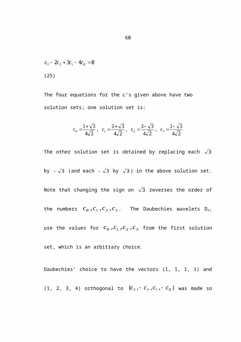
121

throughs, where resolution of individual objects increases or decreases depending on

how close or how far the viewer is from the object. A disadvantage is that the method

is slower since the entire hierarchy must be constructed for the model beforehand.

Another disadvantage is that although the method is useful for one or a few objects, it

does not work so well for a complex scene which contains several different objects.

7.4. Space Applications

Use of image compression in space applications must deal with additional constraints

not present in other applications. The compression technique must be scalable to the

type of image used (eg. visible, infrared), the compression method must be adaptable

to images from moving satellites that use a continuous, or push-broom scan, and the

compression method must use a minimal amount of electrical power [25].

An organization known as IMEC [25] uses wavelet based compression techniques,

which are complex, but satisfy the above constraints. In 1998, the OZONE chip,

which is the first compression chip for wavelet transformed images, was introduced.

In Spring 2002, the FlexWave II chip was demonstrated, which has much higher pro-

cessing throughput than the OZONE chip and handles multiple wavelet configur-

ations. The FlexWave II architecture is shown in Figure 70.

Figure 70. FlexWave II architecture (Taken from [25])

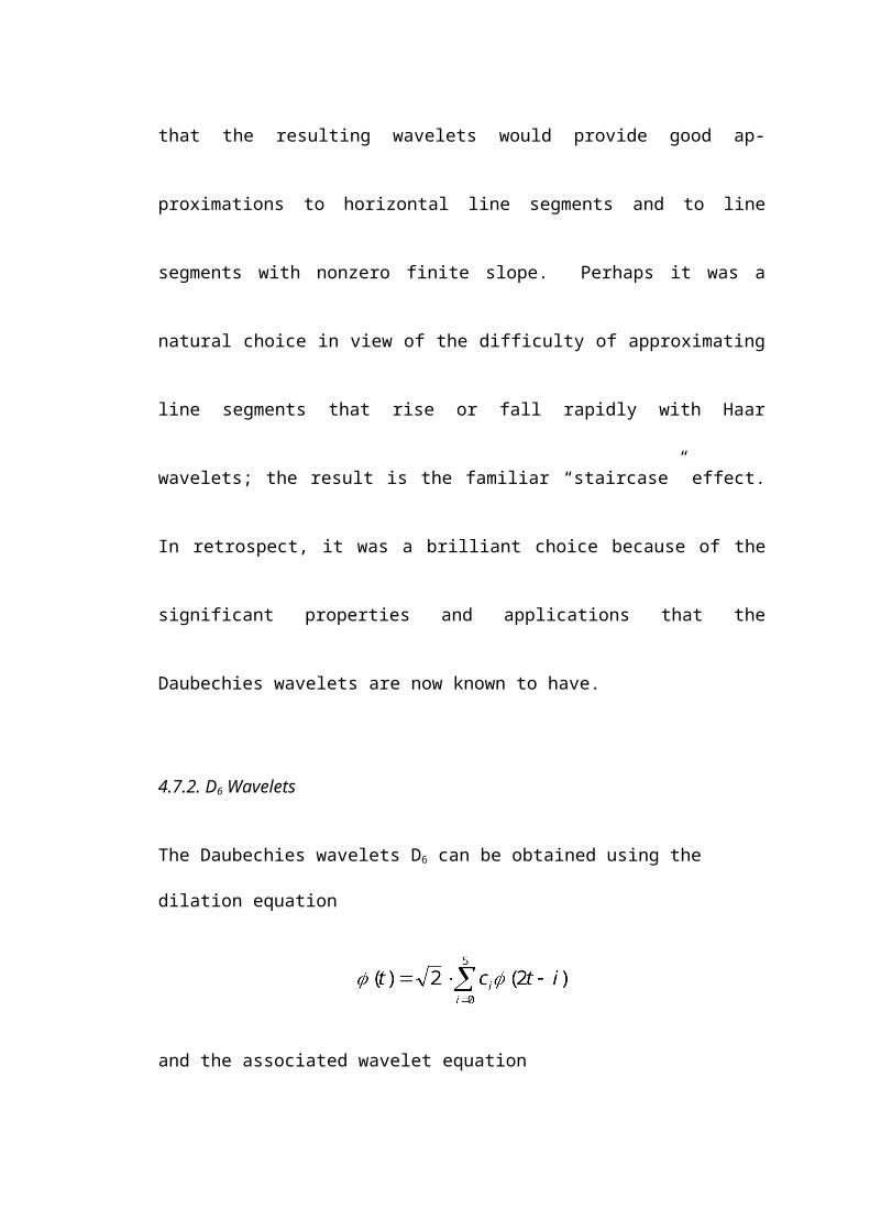
122Another space organization, CCSDS (Consultative Committee for Space Data Sys-

tems) [28] also uses wavelet based image compression, along with a bit-plane en-

coder. Figure 71 shows results from compressing an image using CCSDS, JPEG, and

Figure 71. Reconstructions of aerial image using CCSDS, JPEG, and JPEG2000 (Taken from [28])

JPEG2000 techniques. The quality of the reconstruction from the CCSDS method is

comparable to that of JPEG2000. Notice that the JPEG version contains blockiness.

7.5. Geophysics and Seismics

An important research project in the geophysics field is the Wavelet X-ray Transform

[20]. It filters 2D seismic data sets, which contain information about the location of

geological features under the earth's surface. These images also contain portions that

123

are irrelevant, such as waves that were generated directly from the explosion. This

wavelet technique is used to separate the relevant portions from those that are

irrelevant, in terms of time, frequency, or direction. Figure 72 shows two images of

the brain, the second one obtained from removing irrelevant information. The resolu-

tion is the same as that of the original.

Figure 72. Brain image, original on left, reconstruction on right (Taken from [20])

Wavelets are also used in analyzing seismograms. Waves arrive at the earth's surface

at different times, which are referred to as phases. A research interest is to find the

different time periods, that is, where the phases are located in the seismogram. This

can be used to distinguish a nuclear explosion from an earthquake, and also locate the

source of a geological event.

7.6. Meteorology and Weather Imaging

The AWIPS (Advanced Weather Interactive Processing System) [26] system gener-

ates as much as 5-8 GB of data per day. There is a growing need for distributed mete-

orological workstations located remotely. Thus, the need for effective image com-

pression schemes is ever more important.

Numerical forecast models make up the largest meteorological data sets. A typical

parameter has a size of 80MB. Compression using lossless techniques can only ach-

124

ieve compression rates of 1.1:1 or 1.5:1. Wavelet lossy techniques can achieve com-

pression rates of 40:1 to 300:1, and also result in minimal error.

There are three main types of weather image data. The first is radar images. In radar

images, every pixel is important, but information is rather sparse, and so lossless tech-

niques can compress the image considerably. The second type of weather image is a

satellite image. For this type of data, wavelet compression is used. The error result-

ing from reconstruction must be visually imperceptible. Wavelet compression tech-

niques can achieve rates of 7:1, 15:1, and 50:1 for visible, infrared, and water vapor

channel images respectively, with very little visual loss. The third type of weather

image is a vector graphics file, which is a graphical representation of observations, or

model output. This type of image can only be compressed using lossless techniques.

Another compression technique often used on weather images is non-uniform com-

pression. This technique focuses on a small region of the image, and basically ignores

the rest. This method is similar to the region of interest encoding used in medical

imaging, and the separating of relevant and irrelevant portions in seismic images.

7.7. Digital Photography

As more and more people use digital cameras, methods of efficient storage become

more of a concern. Until a digital camera is full, images can be stored in it losslessly.

When the camera becomes full, images can be compressed using lossy techniques in

order to fit additional images. This will likely sacrifice image quality. If extreme

high quality is necessary, then the user could load the images onto a computer from

the camera while they were still stored in lossless mode. If quality is not a main con-

cern, then lossy techniques can be used to store many more images in the camera.

The JPEG2000 method produces much higher quality images than previous compres-

sion techniques, even with lossy compression [6].

1257.8. Internet/E-Commerce

The amount of business done on the Internet is increasing very rapidly. The need for

effective image compression techniques in e-commerce, then, becomes more and

more important. Often, a user wishes to view an image of a product before they pur-

chase it. On some websites, images are displayed as small thumbnails, which can be

enlarged by clicking on them. Older methods of compression used a separate file for

each of the small thumbnail and the enlarged image, each having a different resolu-

tion. If the JPEG2000 method is used, then the same image file can be used for all

purposes. The JPEG2000 uses the wavelet transform, which represents the image at

multiple levels of resolution, resulting in progressive refinement. JPEG2000 also

yields better image quality than earlier methods [6].

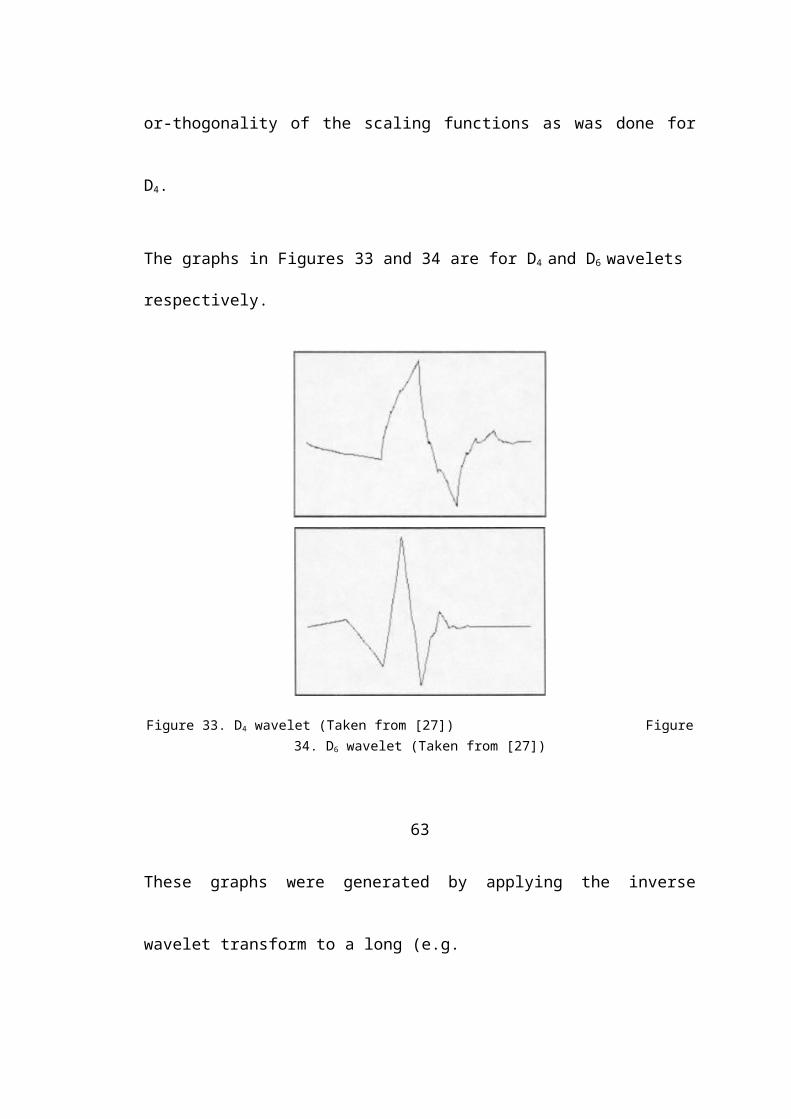
126

Appendix: Proofs of Theorems

Proof of Theorem 1

The normalized general dilation and wavelet equations imply that and

span a subspace of the two-dimensional subspace of spanned by

and . Since the supports of and are disjoint

intervals of length , their product is the zero function. Then using the equation

yields

Therefore,

Thus, and are orthogonal and hence linearly independent.

Consequently, and span a two-dimensional subspace that is

contained in the two-dimensional subspace spanned by and .

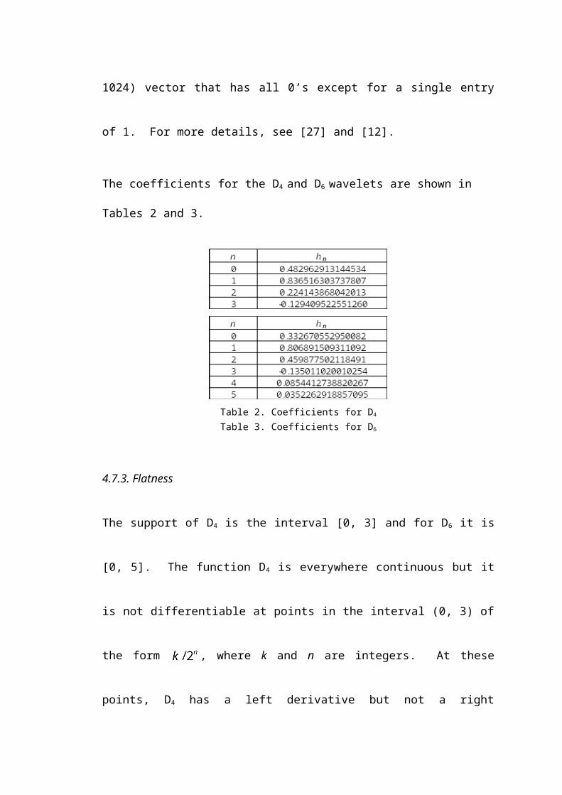
Therefore, and span the same subspace as do and

.

127Proof of Theorem 2

Theorem 1 with k = 0 implies that , ,

is an orthogonal basis for . Then Theorem 1 with k = 1 implies that ,

, , , is an orthogonal basis

for . Since in Theorem 1, the maximum value for k is

. Continuing to apply Theorem 1 for successive values of k until yields

as a basis for . Functions with disjoint support are orthogonal, so the

functions in are orthogonal, the functions in are orthogonal, and a

function in is orthogonal to a function in when k ≠ l.

This leaves the function pairs and which are orthogonal by

Theorem 1.

Proof of Theorem 3

It is only necessary to show that there are functions in the set

and that these functions are orthogonal. The support of a

wavelet at level i, say , is one of the subintervals of length obtained by

partitioning the interval [0, 1) into non-overlapping subintervals of equal length.

At level i + 1 the support of the wavelets are

obtained by dividing each of the subintervals at level i into two equal parts. Thus, the

support of a wavelet at level i + 1 is contained in either the left half or the right half of

a unique subinterval at level i, which in turn is contained in either the left half or the

right half of a subinterval at level i – 1, …. Furthermore, a wavelet has the value 1 on

the left half of its support (including the left endpoint but not the right endpoint) and

the value –1 on the right half of its support (including the left endpoint but not the

128

right endpoint). Therefore, two wavelets at different levels have either disjoint sup-

ports, in which case they are orthogonal, or else the support of the wavelet with the

higher numbered level is contained in a portion of the support of the other wavelet

where that wavelet is constant, so again the two wavelets are orthogonal. Obviously,

all wavelets at the same level are orthogonal since their supports are disjoint. Also,

all wavelets are orthogonal to the function which is constant on the interval

[0, 1). Therefore, the functions listed in the theorem are

orthogonal.

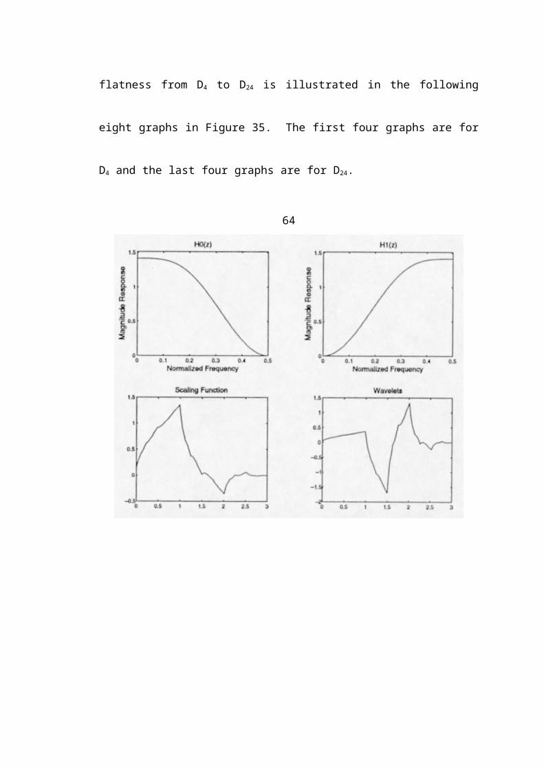
129

References

[1] Ahmed, N., Natarajan, T., Rao, K.R. Discrete Cosine Transform. IEEE Transactions on Computers, Jan. 1974. pp. 90-93.

[2] Aware, Inc. JPEG2000 for Medical Applications. http://www.aware.com/products/compression/jpeg2000_med.html

[3] Brislawn, C. The FBI Fingerprint Image Compression Standard. June 2002. http://www.c3.lanl.gov/~brislawn/FBI/FBI.html

[4] Daubechies, I. Orthonormal Bases of Compactly Supported Wavelets. Communications on Pure and Applied Mathematics, 1988. pp. 909-996.

[5] Daubechies, I. Ten Lectures on Wavelets. CBMS61, SIAM Press, Philadelphia, PA, 1992.

[6] Elzinga, J., Feenstra, K. Applications of JPEG2000. Dec. 2001. http://www.gvsu.edu/math/wavelets/student_work/EF/applications.html

[7] Haar, A. Zur Theorie der Orthogonalen Funktionen – System, Math. Ann., 1910. pp. 331-337.

[8] Information and Communication Theory Group, VcDemo: Image and Video Compression Learning Tool. TU-Delft. http://www-ict.its.tudelft.nl/~inald/vcdemo

[9] Mahoney, D. Big Pictures, Little Packages. Computer Graphics World, May 2001. http://cgw.pennnet.com/Articles/Article_Display.cfm?&Section=Articles&SubSection=Display&ARTICLE_ID=99510&PUBLICATION_ID=18&VERSION_NUM=1

[10] Mulcahy, C. Image Compression Using the Haar Wavelet Transform. Spelman Science and Math Journal, Spring 1997. pp. 22-31.

[11] Nijhuis, G. Introduction to Image Compression. http://www.laesieworks.com/digicom/Intro.html

[12] Press, W., Teukolsky, S., Vetterling, W., Flannery, B. Numerical Recipes in C, Second Edition. Cambridge University Press, 1992.

130[13] Saha, S. Image Compression - from DCT to Wavelets: A Review. ACM Crossroads Students Magazine, 2000.http://www.acm.org/crossroads/xrds6-3/sahaimgcoding.html

[14] Said, A., Pearlman, W. A New, Fast, and Efficient Image Codec Based on Set Partitioning in Hierarchal Trees. IEEE Transactions on Circuits and Systems for Video Technology, June 1996. pp. 243-250.

[15] Shapiro, J. Embedded Image Coding Using Zerotrees of Wavelet Coefficients. IEEE Transactions on Signal Processing, Dec. 1993. pp. 3445-3462.

[16] Silicon Imaging MegaSAVE. Introduction to SPIHT. http://www.siliconimaging.com/SPIHT.htm

[17] Strang, G. Wavelets. American Scientist, April 1994. pp. 250-255. (Also appears as Appendix 1 of Strang [19].)

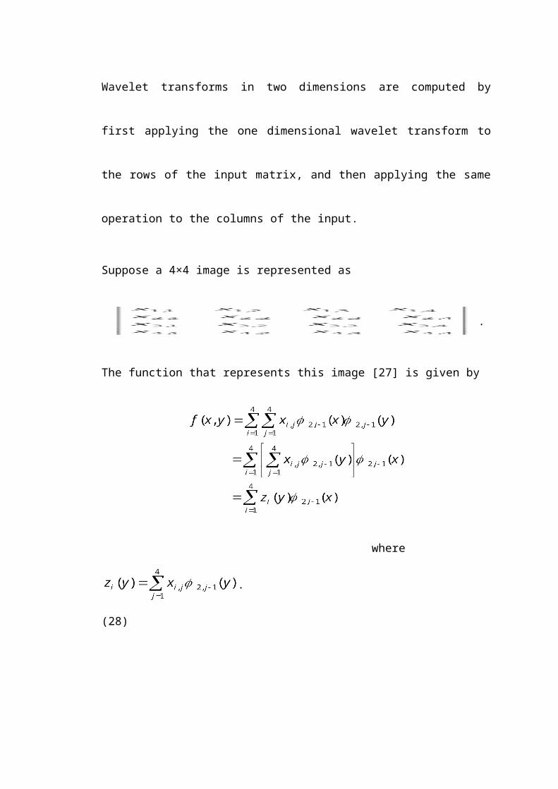
[18] Strang, G. Wavelets and Dilation Equations. SIAM Review, 1989. pp. 613-627. (Also appears as Appendix 2 of Strang [19].)

[19] Strang, G., Nguyen, T. Wavelets and Filter Banks. Wellesley-Cambridge Press, Wellesley, MA, 1996.

[20] Temme, N. The Use of Wavelets in Seismics and Geophysics. ERCIM News, July 1998. http://www.ercim.org/publication/Ercim_News/enw34/temme.html

[21] UNESCO. Arithmetic Coding. 1999-2000.http://www.netnam.vn/unescocourse/computervision/107.htm

[22] UNESCO. Huffman Coding.1999-2000. http://www.netnam.vn/unescocourse/computervision/103.htm

[23] Usevitch, B. A Tutorial on Modern Lossy Wavelet Image Compression: Foundations of JPEG2000. IEEE Transactions on Signal Processing, Sept. 2001. pp. 22-35.

[24] Valens, C. EZW Encoding. 1999-2004. http://perso.wanadoo.fr/polyvalens/clemens/ezw/ezw.html

[25] Waelkens, C. IMEC implements efficient image compression for ESA. Vlaamse Ruimtevaart Industrielen Newsletter, July 2002.http://www.vrind.be/en/newsletter-n2j7.htm

131[26] Wang, N., Madine, S., Brummer, R. Investigation of Data Compression Techniques Applied to AWIPS Datasets. NOAA Research - Forecast Systems Laboratory, Jan. 2004. http://www-id.fsl.noaa.gov/w4_comptech.html

[27] Welstead, S. Fractal and Wavelet Image Compression Techniques. SPIE - The International Society for Optical Engineering, Bellingham, WA, 1999.

[28] Yeh, P., Venbrux, J. A High Performance Image Data Compression Technique for Space Applications. 2003.

132