17-163

3-Dimensional acoustic measurements — using gating techniques

by Henning Meller Bruel & Kjaer

1. Abstract The subjective listening impres- measurement" of the various acous- some experience to interpret the 3D

sion in a room is a function of many tic surfaces using a gated sine tone results just as it requires more expe-acoustic qualities. The more parame- burst, and then to a "3-d imen- rience to interpret a frequency re-ters that can be viewed at the same sional" plot of how the various fre- sponse than a single number on a t ime, the easier it is to evaluate the quency responses change as func- voltmeter. objective qualities of the room. tion of time when the reflections ar­

rive. The 3D plots are obtained us- The paper wil l show the influence This paper wil l therefore try to ex- ing a gated pink noise pulse, a Real- of various time resolutions and fre-

pand the traditional "1-d imen- Time Analyzer, a calculator and a quency resolutions as well as rec-siona!" acoustic reverberation time digital plotter. tangular and Gaussian time weight-measurement — first, to a "2-d i - ings. mensional frequency response However, it requires, of course,

2. Principle of Gating Techniques — using Swept Tone Bursts One of the basic problems in

room acoustic measurements has al­ways been to determine the direc­tion of a certain reflection, and more important, its frequency con­tent. For example, what is the acoustic influence of a certain type of ceiling structure and surface in a concert hall or a studio.

Gating techniques are a simple so­lution to these problems. Gating is a selective measurement in the time domain just as frequency analy­sis is a selective measurement in the frequency domain. A tone burst is transmitted from a loudspeaker and measured at the listening posi­tion as indicated in Fig.1 .

F i g . l . Principle of gated measurements

The simple implementation of this measurement is as described in the 1975 paper (Ref.1) — a swept sine that is cut into tone bursts at the zero crossings. The instrument set­up is shown in Fig.3 and the t ime and frequency spectra of the tone bursts are shown in Fig.4. The out­put of the Sine Generator 1023 is passed through the transmitt ing sec­tion of the Gating System 4 4 4 0 and transformed into a tone burst of adjustable length (0,1 ms to 1 s) which then is fed through the power amplifier to the loudspeaker. The signal received by the micro­phone passes through the Measur­ing Amplif ier to the receiving sec­tion of the Gating System where the desired portion of the signal is selected by the measuring gate, whose width and delay are also ad­justable over a wide range. A peak detector measures the amplitude of the desired signal and feeds a DC voltage proportional to this value to the Level Recorder which is syn­chronized wi th the Sine Generator for automatic recording of fre­quency response. The peak detector contains a hold circuit which is reset for each new tone burst to per­mit capturing the new amplitude as the frequency changes. To monitor the adjustment of the Gating Sys­tem, a two-channel oscilloscope is essential.

The restriction on lower l imit ing frequency is related to the size of the room, as is the case for ane-choic rooms. A detailed description of this can be found in the 1975 paper (Ref.1).

The transmission of the tone burst wi l l (as indicated in Figs. 1 and 2) result in a direct received sig­nal that obviously wi l l arrive f irst, fol lowed by a number of bursts corresponding to the reflections from the various surfaces.

In the 1975 paper (Ref.1) we em­phasized the measurement of the di­rect sound that only contains the free-field information of the loud­speaker itself, whi le this paper wi l l concentrate on the measurement of the reflections in order to obtain in-

2

Fig.4. Time and frequency spectra of gated sine wave. Notice that a narrow time spectrum corresponds to a broad frequency spectrum and vice versa

formation about the acoustic pro- gate is adjusted so it only picks up perties of the room. The measure- the information corresponding to a ment set-up is essentially the same particular acoustic surface. as in Fig.3 except the measuring

Fig.3. Set-up using Gating System

Fig.2. Reflections f rom the environment

3

3. Measurements of Frequency Response of Acoustic surfaces — using Gating Techniques with Swept Sine Bursts

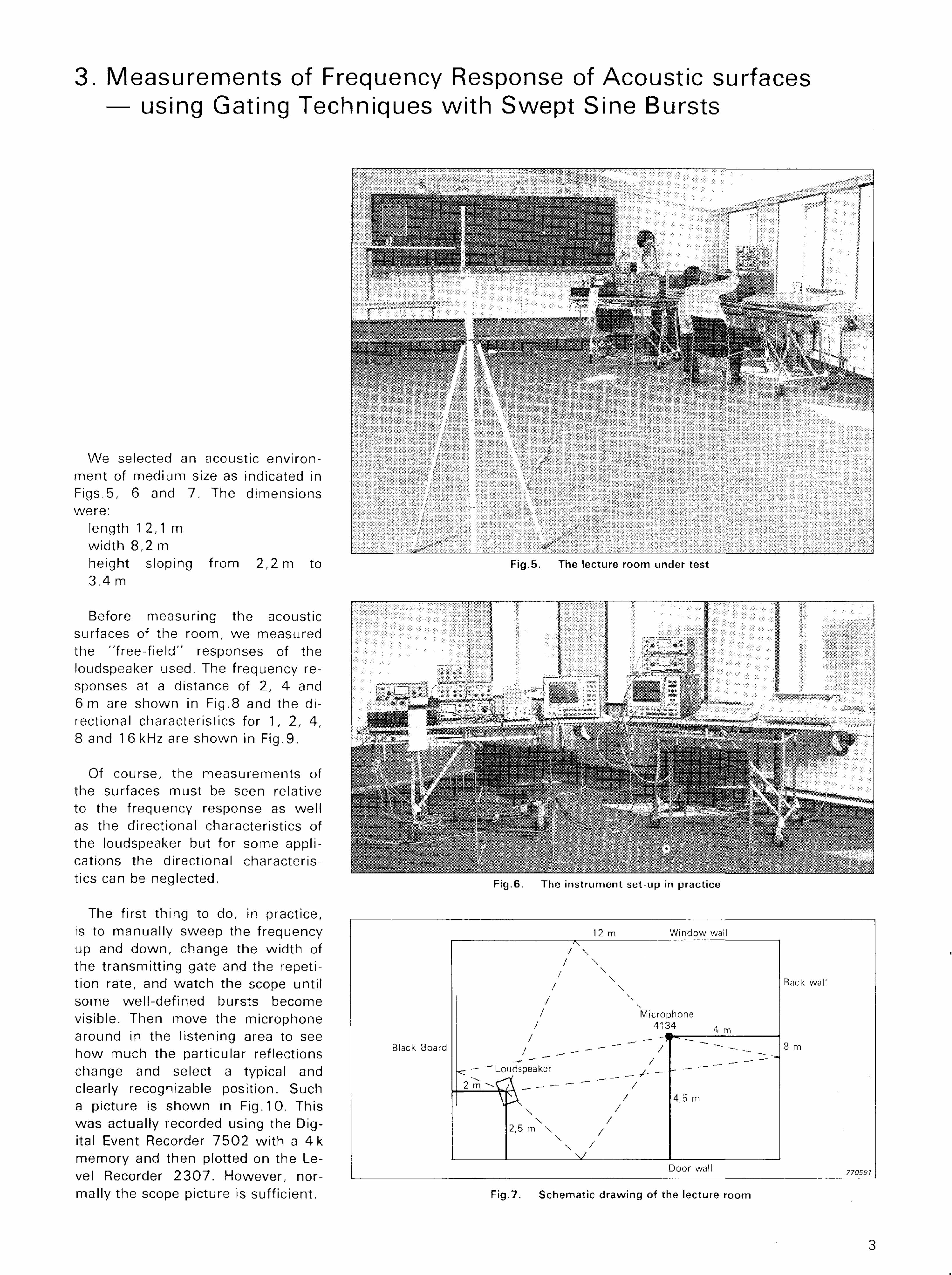
We selected an acoustic environ­ment of medium size as indicated in Figs.5, 6 and 7. The dimensions were:

length 1 2 , 1 m width 8,2 m height sloping from 2,2 m to 3 , 4 m

Before measuring the acoustic surfaces of the room, we measured the " f ree- f ie ld" responses of the loudspeaker used. The frequency re­sponses at a distance of 2, 4 and 6 m are shown in Fig.8 and the di­rectional characteristics for 1 , 2, 4 , 8 and 1 6 kHz are shown in Fig.9.

Of course, the measurements of the surfaces must be seen relative to the frequency response as well as the directional characteristics of the loudspeaker but for some appli­cations the directional characteris­tics can be neglected.

The first thing to do, in practice, is to manually sweep the frequency up and down, change the width of the transmitt ing gate and the repeti­tion rate, and watch the scope until some well-defined bursts become visible. Then move the microphone around in the listening area to see how much the particular reflections change and select a typical and clearly recognizable position. Such a picture is shown in Fig.10. This was actually recorded using the Dig­ital Event Recorder 7 5 0 2 wi th a 4 k memory and then plotted on the Le­vel Recorder 2 3 0 7 . However, nor­mally the scope picture is sufficient.

Fig.5. The lecture room under test

Fig.6. The instrument set-up in practice

Fig.7. Schematic drawing of the lecture room

The most prominent reflections for the selected loudspeaker-micro­phone position are indicated in Fig.10 using a 3 1 3 0 Hz tone burst of 1,6 ms width. It can be seen that at this frequency the "Black Board reflection" is slightly out of phase wi th reflection from the wall behind it — and the direct sound and the reflections from them there­fore is quite small.

However, ceil ing/f loor, the door wal l , the window wal l , and the back wall are clearly visible. The black­board reflection can clearly be seen by changing the frequency slightly.

4

Fig. 10. The t ime funct ion of the various reflections in the lecture room recorded on the Digital Event Recorder 7 5 0 2 and plotted on the Level Recorder 2307

Fig.9. Directional characteristics of the loudspeaker used

Fig.8. "Free- f ie ld" measurements of the loudspeaker used

To determine which reflections correspond to the various surfaces, simple geometry can be used as in­dicated in Fig.7. However, in prac­tice, it wi l l often be easier to use an acoustic screen (this Application Note wil l work quite well) and manu­ally positioning this between the microphone and the various reflect­ing surfaces and watching the scope until only one of the bursts disappears. When that happens the reflecting surface is determined.

The next step is to measure the "frequency responses" correspond­ing to the various surfaces. These responses must, of course, be seen as the difference between the direct (or free-field sound transmitted from the loudspeaker) and the ref­lected sound. This is done by manu­ally adjusting the measuring gate so it only picks up the response corre­sponding to one of the surfaces at a t ime, (for instance, as indicated in Fig.10 — the door wal l informa­tion), and then start the automatic sine sweep. The results of these measurements are shown relative to the frequency response in Figs.1 1, 12, 13 and 14.

First of al l , it is seen that most of the reflections on average are about 10dB down, but they do not die down at the same rate at all fre­quencies. Since the four curves are different, they also indicate that the decay rates at the various frequen­cies are different in the different di­rections.

The most pronounced "p rob lem" is probably the w indow wal l and back wal l reflections at 2—3 kHz (Figs.1 3 and 14) that show a signif i­cant " f lut ter echo" since the ref­lected signals are only approxi­mately 1 dB down after 1 5 ms and 24 ms respectively.

Obviously, the t ime picture (Fig. 10) doesn't reveal the fre­quency information and the fre­quency pictures (Figs.1 1 —14) don't show the t ime information. The so­lution therefore is a 3D plot of the frequency spectra as a funct ion of t ime. This is virtually impossible to do manually but is quite easy using modern programmable calculators.

5

Fig.12. The reflected sound f rom the door wall relative to the direct sound f rom the loud­speaker

* Fig.13. The reflected sound f rom the w indow wal l relative to the direct sound f rom the loud­speaker

■ - ^ ■ - _ - _ -^ — J

Fig-11, The reflected sound from the ceiling and floor relative to the direct sound f rom the loudspeaker

4. Instrument set-up for 3D Measurements In recent years, there have been The Sine Generator 1023 is re- Frequency Analyzer 2 1 2 0 is just

several approaches in the audio in-- placed by the Noise Generator used as a high pass filter in order to dustry to introduce 3D plots, 1405 since the frequency analysis avoid the low frequencies that make (Rets.2—6) but the expense so far is done by the Digital Frequency An- the scope picture unstable. It also has been considerable. But modern alyzer 2 1 3 1 . The first Gating Sys- removes the low frequency informa-instruments and calculators con- tern 4 4 4 0 operates as a transmit- tion which is measured wi th too nected via the SEC digital interface ting gate that in this case cuts the much statistical uncertainty to be bus make these measurements pos- pink noise into bursts at the zero useful due to the narrow measuring sible at a reasonable price using the crossings. The width is manually ad- gate. A further discussion of the re-traditional "2D instruments" as the justable in the range 0,1 ms to lation between frequency resolution hardware basis. The instrument set- 1 s. The gated pink noise pulse is and time resolution follows in see-up used for this application is introduced to the loudspeaker and tion 5. shown in Fig. 1 5. picked up by the microphone. The

Fig.14. The reflected sound from the back wal l relative to the direct sound f rom the loud­speaker

Fig. 15. The instrument set-up using gated pink noise, real-time analysis and automatic control by calculators

6

:- Fig.16. Setting of gates to measure the various reflections w i th the set-up in Fig.15

The second Gating System is used as an analogue measuring gate (Fig. 16) which is required since the normal built- in measuring gate only measures the highest posi­tive peak that was in the signal whi le the measuring gate was open. In other words the gated infor­mation is only available as a DC vol­tage when only one Gating System 4 4 4 0 is used; but it is available as an analogue voltage, that can be fre­quency analyzed, when two Gating Systems are used. A Gauss Mul t i ­plier is also usable as described in section 8. This set-up can, of course, be manually operated as in­dicated in Figs. 15 and 16 using the measuring gate of the first Gating System as a trigger for the other Gating System. By manually chang­ing the delay of the receiving gate of the first Gating System (the tr ig­ger position) and thereby the posi­tion of the analogue measuring gate (the transmission gate of the sec­

ond gating system) different parts of buffer amplif ier is necessary to the received signal can be analyzed, drive the Gating Systems from the and it can be seen how the fre- IEC bus; or the Gating Systems can quency spectra change wi th t ime. be modified for a higher input im­

pedance.) However the strong feature of the

system is that it can be automati- Depending on the software used, cally controlled using a calculator. we can now automatically control There are many of these on the mar- the start of the transmission burst ket but B & K recommend either the (Gating System No.1) and the start HP 9 8 2 5 A and the Digital Plotter of the receiving gate (Gating Sys-HP 9 8 7 2 A or the Tektronix 4 0 5 1 . tern No. 2). The widths of the trans-These both use the IEC interface mission gate and the receiving gate bus that most new B & K instru- are manually adjustable on the two ments are equipped w i t h . (Note: a gating systems.

Fig.18. 3 D plot of lecture room showing how the frequency spectra change w i th t ime. 0—50 ms t ime axis. Receiving gate 4,7 ms

Typical results of this measure- tively, and they show how the fre- along the frequency axis. Stated ment are shown in Figs. 17—22. quency spectra change with time another way, a short gate gives

over the 0 to 50 ms time span. good time resolution while a long The first three plots, Figs. 17, 18 gate gives good frequency resolu-

and 19 are building acoustics meas- It is seen that the very narrow t ion. urements using the loudspeaker- measuring gate (1,5 ms) used in microphone position indicated in Fig.17 displays a visible wave struc- The "flutter echo" we noticed us-Fig.5 and Fig.7. The three plots are ture in the 3D spectrum travelling ing the simple gated sine wave essentially the same but wi th differ- along the time axis, whi le the (Figs.13 and 14) is clearly visible in ent time resolutions in the receiving measuring gate (15ms —Fig.19) Fig.19 but not very obvious in gate: 1,5, 4,7 and 15 ms respec- shows a wave structure travelling Fig.1 7 and Fig.1 8.

8

Fig. 17. 3 D plot of lecture room showing how the frequency spectra change wi th t ime, 0—50 ms time axis. Receiving gate 1,5 ms

5. 3D plots of how the Frequency Spectra change with time

Fig. 19. 3 D plot of lecture room showing how the frequency spectra change wi th t ime. 0—50 ms time axis. Receiving gate 15 ms Notice the "Flutter Echo" at 2 kHz

As previously seen in Figs. 17 to F _ _ 1 _ whenever making this kind of meas-22 , the appearance of the 3 D spec- T urement. They are equally appli-trum depends on the width of the re- cable for digital and analog filters, ceiving gate. One may then ask, For example, if the receiving gate is FFT (Ref.13), and any other what gate width should be used to 5 ms (=T), then the frequency reso- method. The "smear" in this type of give the correct result. The answer lution is 200 Hz. However, even measurement is a result of a law of is: "That depends on what informa- though the receiving gate is 5 ms nature that you can't cheat. tion you want . " If good time resolu- long, we can move it in much tion is desired, a very narrow time smaller increments — and what we Since pink noise, which is a ran-window must be used — but this see is how a given frequency com- dom signal, was used for these has the unavoidable by-product of ponent changes as a function of measurements, a certain amount of giving very poor frequency resol- time — with a "spreading out" of averaging is necessary to get reprod-t ion. On the other hand, if good fre- the signal over a 5 ms interval. Ri- ucible results. For these measure-quency resolution is desired, the chard C. Heyser has called this a ments, averaging was performed time resolution wil l be reduced. The "t ime smear" (Ref.7—9). These res- over 15 noise bursts using a 4 s av-mathematical relationship is very trictions on time and frequency reso- eraging time in the Digital Fre-simple: lution should be kept firmly in mind quency Analyzer 2 1 3 1 .

9

F ig .21 . 3 D plot of Early Reflections of loudspeaker. Time 0—8 ms. 1 ms 1,2 kHz tone burst

10

Fig.20. 3 D plot of Early Reflect ion of loudspeaker. Time 0—8 ms. 1 ms 9,9 kHz tone burst

6. Early reflections of the Loudspeaker used The 3D technique is also appli- Figs. 17—19. In this case (Figs.20- cially in the cabinet. It indicates

cable to the so-called "Early reflec- 22) from 0—8 ms. how fast the response of the sys-t ions" that describe how the fre- tem is and how much sound of its quency response changes wi th t ime Early reflections are due to over- own the loudspeaker box adds to for the loudspeaker itself. In other hang of the speaker, and reflec- the signal. words, the first few mill iseconds of t ions, standing waves, and reson-the curves previously displayed in ances in the speaker itself and espe- Here again it's a question of the

optimum trade-off between fre- Fig.22 we have used a 1 ms gated mitting signal the time resolution is quency and time resolution. In pink noise pulse and still a receiv- more clearly visible. It is simply Fig.20 we have a 1 ms 9,9 kHz ing gate of 0,4 ms. equivalent to the scope picture, but tone burst and a receiving gate of the disadvantage is that it doesn't si-0 ,4ms. In Fig.21 we have used a Obviously when only one fre- multaneously show the behaviour 1 ms 1,2kHz tone burst and a re- quency (and its sidebands because of the other frequencies as Fig.22 ceiving gate of 0,4 ms and in of the gating) is used as the trans- where we used gated pink noise.

Fig.22 3 D plot of Early Reflections of loudspeaker. Time 0—8 ms. 1 ms pink noise tone burst

12

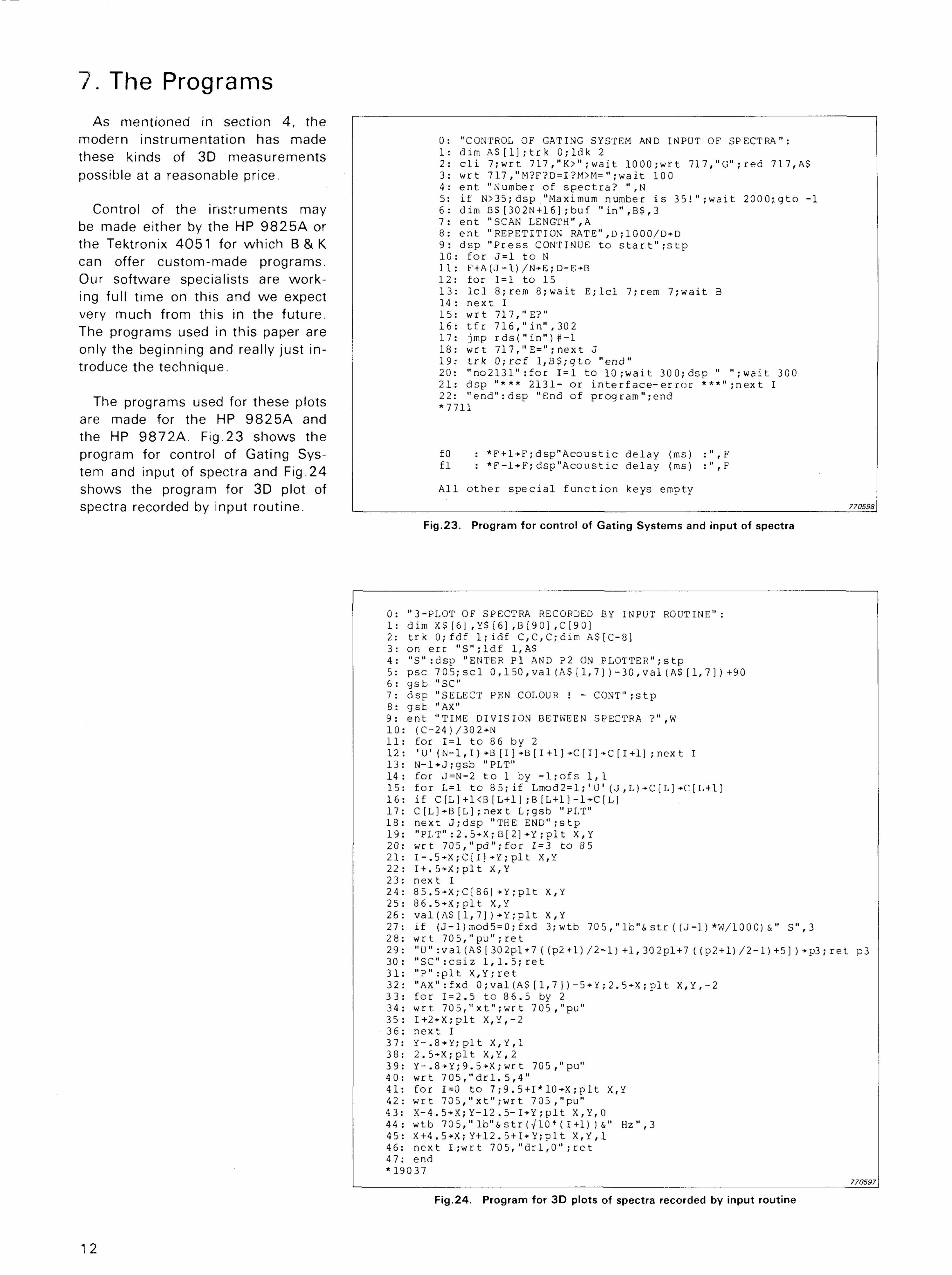
7. The Programs As mentioned in section 4 , the

modern instrumentation has made these kinds of 3D measurements possible at a reasonable price.

Control of the instruments may be made either by the HP 9 8 2 5 A or the Tektronix 4051 for which B & K can offer custom-made programs. Our software specialists are work­ing full t ime on this and we expect very much from this in the future. The programs used in this paper are only the beginning and really just in­troduce the technique.

The programs used for these plots are made for the HP 9 8 2 5 A and the HP 9872A . Fig.23 shows the program for control of Gating Sys­tem and input of spectra and Fig.24 shows the program for 3D plot of spectra recorded by input routine.

Fig.23. Program for control of Gating Systems and input of spectra

Fig.24. Program for 3D plots of spectra recorded by input routine

0 : "CONTROL OF GATING SYSTEM AND INPUT OF SPECTRA": 1 : d im A S [ 1 ] ; t r k 0 ; l d k 2 2: cli 7;wrt 717,"K>";wait 1000;wrt 717,"G";red 717,A$ 3: wrt 717,"M?F?D=I?M>M=";wait 100 4 : e n t "Number of s p e c t r a ? " , N 5: i f N > 3 5 ; d s p "Maximum number i s 3 5 ! " ; w a i t 2 0 0 0 ; g t o - 1 6 : dim B S [ 3 0 2 N + 1 6 ] ; b u f " i n " , B $ , 3 7 : e n t "SCAN LENGTH",A 8 : e n t "REPETITION R A T E " , D ; 1 0 0 0 / D - D 9 : d s p " P r e s s CONTINUE t o s t a r t " ; s t p 1 0 : f o r J = l t o N 11 : F + A ( J - 1 ) /N+E;D-E-<-B 1 2 : f o r 1=1 t o 15 1 3 : l e i 8 ; r e m 8 ; w a i t E ; l c l 7 ; r e m 7 ; w a i t B 14 : n e x t I 1 5 : w r t 7 1 7 /

, , E ? " 1 6 : t f r 7 1 6 , " i n " , 3 0 2 1 7 : jmp r d s ( " i n " ) # - 1 1 8 : w r t 7 1 7 , " E = " ; n e x t J 1 9 : t r k 0 ; r c f l , B $ ; g t o " e n d " 2 0 : " n o 2 1 3 1 " : f o r 1=1 t o 1 0 ; w a i t 3 0 0 ; d s p " " ; w a i t 300 2 1 : d s p " * * * 2 1 3 1 - o r i n t e r f a c e - e r r o r * * * " ; n e x t I 2 2 : " e n d " : d s p "End o f p r o g r a m " ; e n d * 7 7 1 1

fO : * F + l + F ; d s p " A c o u s t i c d e l a y (ms) : " , F f l : * F - 1 + F ; d s p " A c o u s t i c d e l a y (ms) : " , F

A l l o t h e r s p e c i a l f u n c t i o n k e y s emp ty

0 : "3-PLOT OF SPECTRA RECORDED BY INPUT ROUTINE": 1 : d im X$ [6] , Y$ [6] , B [ 9 0 ] , C [ 9 0 ] 2 : t r k 0 ; f d f 1 ; i d f C , C , C ; d i m A $ [ C - 8 ] 3 : on e r r " S " ; l d f 1,A$ 4 : " S " : d s p "ENTER P i AND P2 ON P L O T T E R " ; s t p 5 : p s c 7 0 5 ; s c l 0 , 1 5 0 , v a l (A$ [ 1 ,7] ) - 3 0 , v a l ( A $ [ 1 , 7 ] ) + 9 0 6 : g s b "SC" 7: dsp "SELECT PEN COLOUR ! - CONT";stp 8: gsb "AX" 9: ent "TIME DIVISION BETWEEN SPECTRA ?",W 10: (C-24)/302+N 11: for 1=1 to 86 by 2 12: 'U'(N-1,I)*B[I]+B[1+1]+C[I]+ C[1+1];next I 13: N-1+J;gsb "PLT" 14: for J=N-2 to 1 by -l;ofs 1,1 1 5 : f o r L = l t o 8 5 ; i f L m o d 2 = l ; ' U ' ( J , L ) * C [ L ] + C [ L + l ] 1 6 : i f C [ L ] + K B [ L + 1 ] ; B ( L + 1 ) - 1 * C [ L ] 1 7 : C [L]*B [ L ] ; n e x t L ; g s b "PLT" 1 8 : n e x t J ; d s p "THE E N D " ; s t p 1 9 : " P L T " : 2 . 5 + X ; B [ 2 ] + Y ; p l t X,Y 2 0 : w r t 7 0 5 , " p d " ; f o r 1=3 t o 8 5 2 1 : I - . 5 + X ; C [ I ] + Y ; p i t X,Y 2 2 : I + . 5 * X ; p l t X,Y 2 3 : n e x t I 2 4 : 8 5 . 5 * X ; C [ 8 6 ] * Y ; p l t X,Y 2 5 : 8 6 . 5 + X ; p l t X,Y 2 6 : v a l { A $ [ 1 , 7 ] ) + Y ; p l t X,Y 2 7 : i f ( J - l ) m o d 5 = 0 ; f x d 3 ; w t b 7 0 5 , " l b " & s t r ( ( J - l ) * W / 1 0 0 0 ) & " S " , 3 2 8 : w r t 7 0 5 , " p u " ; r e t 2 9 : "U" : v a l ( A S [ 3 0 2 p l + 7 ( ( p 2 + l ) / 2 - l ) + l , 3 0 2 p l + 7 ( ( p 2 + l ) / 2 - l ) + 5 ] ) + p 3 ; r e t p3 3 0 : " S C " : c s i z 1 , 1 . 5 ; r e t 3 1 : " P " : p l t X , Y ; r e t 3 2 : " A X " : f x d 0 ; v a l ( A $ [ 1 , 7 ] ) - 5 + Y ; 2 . 5 * X ; p i t X , Y , - 2 3 3 : f o r 1 = 2 . 5 t o 8 6 . 5 by 2 3 4 : w r t 7 0 5 , " x t " ; w r t 7 0 5 , " p u " 3 5 : I + 2 + X ; p l t X , Y , - 2 3 6 : n e x t I 3 7 : Y - . 8 + Y ; p i t X , Y , 1 3 8 : 2 . 5 * X ; p l t X , Y , 2 3 9 : Y - . 8 > Y ; 9 . 5 * X ; w r t 7 0 5 , " p u " 4 0 : w r t 7 0 5 , " d r l . 5 , 4 " 4 1 : f o r 1=0 t o 7 ; 9 . 5 + 1 * 1 0 - X ; p l t X,Y 4 2 : w r t 7 0 5 , " x t " ; w r t 7 0 5 , " p u " 4 3 : X - 4 . 5 + X ; Y - 1 2 . 5 - I + Y ; p l t X , Y , 0 4 4 : w t b 7 0 5 , " l b " & s t r ( V l O * ( I + D )&" H z " , 3 4 5 : X + 4 . 5 + X ; Y + 1 2 . 5 + I * Y ; p l t X , Y , 1 4 6 : n e x t I ; w r t 7 0 5 , " d r 1 , 0 " ; r e t 4 7 : end * 1 9 0 3 7

770598 " ■■ - ™ 1 . I I

Fig.27. The operation of the Gauss Impulse Multiplier 5623

13

Fig.26. Electrical response of the system using Gaussian w indow

Fig.25. Difference spectrum between loudspeaker response using Rectangular and Gaussian weightings respectively. Recorded on the Digital Frequency Analyzer 2131 in the fast comparing mode

8. Gaussian or Rectangular Weighting? Pressure or Free-field Microphone?

There are several technical mea­suring problems involved using pulse techniques. The most obvious problem is the sidebands introduced using gating technique. This prob­lem is described in greater detail in the 1975 paper (Ref.1).

The second consideration could be: what kind of weighting function should be used — if any. This is de­scribed in detail in Bob Randall's Ap­plication Note (Ref.10). However us­ing the 1/3 octave resolution the in­fluence of the weighting function is almost negligible as can be seen from Figs.25 and 26.

Fig.25 shows the difference be­tween the rectangular weighting and the Gaussian weighting using a 5 ms burst of pink noise on the loudspeaker and it is seen that from approximately 500 Hz and up the difference is almost constant. The difference spectrum is recorded us­ing the Digital Frequency Analyzer 2131 in the Fast comparing mode while reading out to the Level Recor­der 2307 . This read-out is ex­tremely fast (paper speed 1 0 mm/sec).

Fig.26 shows the electrical re­sponse of the system using the Gauss Impulse Multiplier 5623 . The 200 Hz roll off is due to the high pass filter in 21 20 .

The operation of the Gauss Im­pulse Multiplier 5623 is shown in Fig.27 and is described in further detail in B & K Application Note 1 1 -194 (Ref.1 1). Another technical question that could be asked is what kind of microphone should be used. The directional characteristics of the 1 / 2 " Free-field microphone 4133 show that at 20 kHz the sen­sitivity from the back (180°) is ap­proximately 10dB down and there­fore we used a Pressure micro­phone 4 1 3 4 at grazing incidence which gives the same sensitivity in all directions in the plane of the di­aphragm and since we are just inter­ested in the difference between the direct and the reflected sound this seems optimum.

14

9. Transmission and Reflection of a Conventional Door

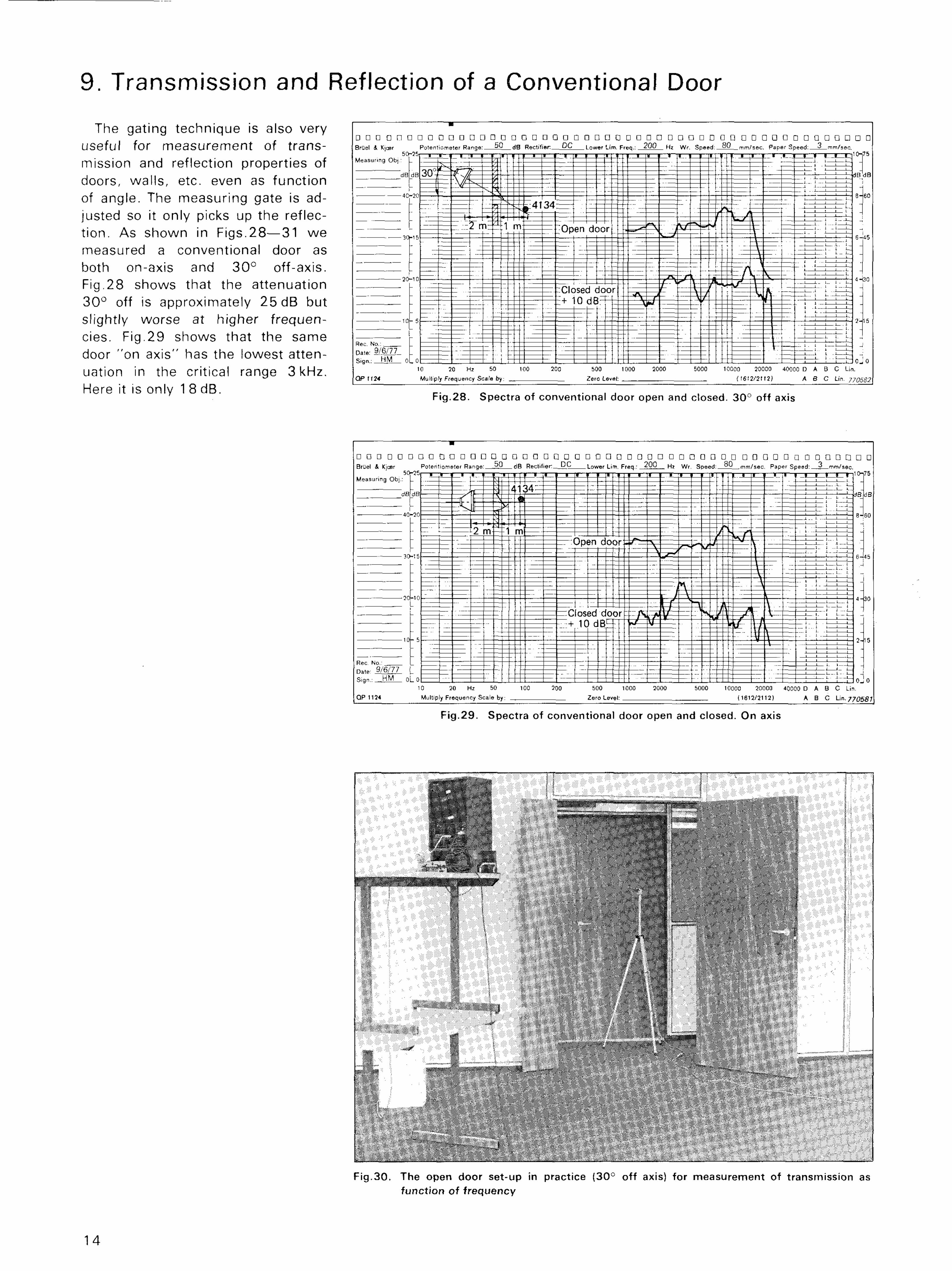
The gating technique is also very useful for measurement of trans­mission and reflection properties of doors, walls, etc. even as function of angle. The measuring gate is ad­justed so it only picks up the reflec­tion. As shown in Figs.28—31 we measured a conventional door as both on-axis and 30° off-axis. Fig.28 shows that the attenuation 30° off is approximately 25 dB but slightly worse at higher frequen­cies. Fig.29 shows that the same door "on axis" has the lowest atten­uation in the critical range 3 kHz. Here it is only 1 8 dB.

Fig.28. Spectra of conventional door open and closed. 30° off axis

F ig.29. Spectra of conventional door open and closed. On axis

F ig.30. The open door set-up in practice (30° off axis) for measurement of transmission as funct ion of f requency

10. Conclusion and Applications

t h I h i | n P at

P e L h a S t r i S d , 0 i n t r 0 d u c e a n 9 ' e i s a n o t h e r important building ment Control Unit 1902 and a sim-the 3D techmque m acoustic and acoustics parameter. pie external A / D converter (Ref 12)

thene°w T / t , a P P " C a t , ° n S U f 9 3 D sound power could also be mea-he new relatively inexpensive calcu- The early reflections of loudspeak- sured and the list is almost endless

lators w,th instruments having an ers in 3D is also an extremely im- enaiess. IEC interface. portant parameter in loudspeaker de- We wi l l conclude the paper by

T h p u „ : | H i n n a ,. . S i g n ' b u t 9 e n e r a l l V t h e 3D program showing two other possibilities us-The building acoustic application can be used for all k.nds of plots in- ing the 3D plots Fig 32 shows the

which is especially emphasized in dicating relations between 3 par- 3D reverberation t ime of t h a T c t u r e this paper is useful ,n concert halls, ameters. A procedure could, for in- room and Fig.33 shows a 1 /12 oc enemas, theatres, studios, etc. stance, be introduced for 3D dis- tave 3D display of the room There

T , a .. t- . p l a y s o f Harmonic, Difference Fre- are many other possibilities in the I he application determining ab- quency and Intermodulation curves future

sorption and reflection coefficients measured wi th the Heterodyne Anal-as a function of frequency and yzer 2 0 1 0 , the Distortion Measure-

15

F ig .31 . Reflections as funct ions of frequency can also be measured using gat ing techniques

16

Fig.33, 1 / 1 2 octave plot of the decay of the lecture room

Fig.32. a) Numerical values of the reverberation t ime in the lecture room b) 3 D plot of reverberation t ime in the lecture room

H u ft b e r o r r e c o r -d i n 3 ■=■"' 31

D r o P f r on Fi a x ■

( i n d 8 ) J l a • j . y

""■ T n

i_ a I c i.41 a .?■ i on i n -t e r '■.' a 1 ( i n dB

r 7 . 6

■ r o. i i o n t i i'i e i n ■■■

C h # i 8 6 :: 9 ■ — .

C h # 19 1 . 0 """F

l . i L J

9 . 7 n

E J 4 4 — — ™ 3 , 6 s I - , -r+ u; ft . b '

0 , ? n

■"■ K # ■"' -■ .-■ ■ i TF i— - yf, 5 r

3 . S h*

i ' -, S -' -?

■_■ : ! t f ::-. i y . 4 L

0 = 4 L

1 . r T ^ - - - V J _ ^ L V V Ifc- . .■ a . 5 r r a 1

" ^ " 1 E J r»r i - y =, 6 _!̂ -

C h # 3 1 6. 6 n

L- r 1 fF O -L- 3. 7 ™ '

r< i- i L ■" ■" S. 7 j

C h # 3 4 @. 8 r 1 - 1 r

C h # 3 ^ 0. 3 J

1

=_■ M tt o - : 0, 8 U - l

I

0= 3 r

L- h If -- o 3. S c

L- r s TT .:= 7 8, 7 ,10

C h # 4 8 T

, " . ™Th L i - - L ■'= 6 i =: :-at e J. 1 :. :■ u I a i ■ I 0 r";

h 0. S 0 t" en i '■ ■ P =: _: Z J l

Ref. 1 speaker wave front propagation Journal of the Audio Engineering Henning M0ller and Carsten Thorn- AES paper, Zurich 1976 Society (AES) sen January 1 9 7 6 Electro Acoustic free-field measure- Ref.6 ments in ordinary rooms — using Suzuki, Mori i and Matsumura, Pion- Ref.10 gating techniques neer, Japan R.B. Randall AES paper New York 1975 or Three-dimensional displays for dem- Frequency Analysis of Stationary, B & K Application Note 1 5—1 07 onstrating transient characteristics Non-stationary and Transient sig-

of loudspeakers nals Ref.2 AES paper, New York 1976 B & K Application Note 14—165 Ole Moller Sorensen Three-dimensional output from Ref .7 Ref. 1 1 Third-octave Frequency analysis Richard C. Heyser Instantaneous Spectrum Analysis B & K Application Note 1 2—1 20 Loudspeaker Phase Characteristics w i th the Real-Time 1 / 3 octave Anal-

and Time Delay Distortion: Part 1 yzer Type 3 3 4 7 Ref.3 January 1 9 6 9 , Part 2 Apri l 1 9 6 9 B & K Application Note 1 1 — 1 94 J . M . Berman Journal of the Audio Engineering Loudspeaker evaluation using digi- Society (AES) Ref.12 tal techniques Carsten Thomsen and Henning AES paper London 1975 Ref.8 M0ller

Richard C. Heyser Swept measurements of harmonic, Ref.4 Determination of Loudspeaker Sig- difference and intermodulation dis-L.R. Fincham, KEF nal Arrival Times: Part 1 October tortion Loudspeaker system simulation us- 1 9 7 1 , Part 2 November 1 9 7 1 , Part B & K Application Note 1 5 — 0 9 8 ing digital techniques 3 December 1971 AES paper London 1975 Journal of the Audio Engineering Ref.13.

Society (AES) Bob Randall Ref.5 Applications of B & K Equipment to Nomoto, Iwahara and Onoye, JVC, Ref.9 Frequency Analysis Japan Richard C. Heyser B & K Technical Book 1 977 A technique for observing loud- Communications

. . . first in Sound and Vibration

Briiel & Kjaer DK-2850 N/ERUM, DENMARK ' Telephone: +45 2 80 05 00 TELEX: 37316 bruka dk