3. Differential Equations - UMD
14
11/1/2011 1 1 Partial Differential Equations Almost all the elementary and numerous advanced parts of theoretical physics are formulated in terms of differential equations (DE). Newton’s Laws Maxwell equations Schrodinger and Dirac equations etc. 2 2 dt x d m ma F Since the dynamics of many physical systems involve just two derivatives, DE of second order occur most frequently in physics. e.g., the steady state distribution of heat acceleration in classical mechanics 2 Ordinary differential equation (ODE) Partial differential equation (PDE) 2 Examples of PDEs • Laplace's eq.: occurs in a. electromagnetic phenomena, b. hydrodynamics, c. heat flow, d. gravitation. • Poisson's eq., In contrast to the homogeneous Laplace eq., Poisson's eq. is non- homogeneous with a source term 2 2 0 k 2 0 2 0 / 0 / The wave (Helmholtz) and time-independent diffusion eqs These eqs. appear in such diverse phenomena as a. elastic waves in solids, b. sound or acoustics, c. electromagnetic waves, d. nuclear reactors.
Transcript of 3. Differential Equations - UMD

11/1/2011
1
1
Partial Differential Equations
Almost all the elementary and numerous advanced parts of theoretical physics are
formulated in terms of differential equations (DE).
Newton’s Laws
Maxwell equations
Schrodinger and Dirac equations etc.
2
2
dt
xdmmaF
Since the dynamics of many physical systems involve just two derivatives,
DE of second order occur most frequently in physics. e.g.,
the steady state distribution of heat
acceleration in classical mechanics
2
Ordinary differential equation (ODE) Partial differential equation (PDE)
2
Examples of PDEs
• Laplace's eq.:
occurs in
a. electromagnetic phenomena, b. hydrodynamics,
c. heat flow, d. gravitation.
• Poisson's eq.,
In contrast to the homogeneous Laplace eq., Poisson's eq. is non-
homogeneous with a source term
2 2 0k
2 0
2
0/
0/
The wave (Helmholtz) and time-independent diffusion eqs
These eqs. appear in such diverse phenomena as
a. elastic waves in solids, b. sound or acoustics,
c. electromagnetic waves, d. nuclear reactors.

11/1/2011
2
3
The time-dependent wave eq.,
Subject to initial and boundary
conditions
Take Fourier Transform
Boundary value problem per freq
• Helmholtz equation
.
dtetzyxpwzyx ti
),,,('),,,(
The time-dependent heat equation
Subject to initial and boundary
conditions
Biharmonic Equation
.
Numerical Solution of PDEs • Finite Difference Methods
– Approximate the action of the operators
– Result in a set of sparse matrix vector equations
– In 3D a discretization will have Nx× Ny× Nz points
– Iterative methods such as multigrid give good performance
• Finite Element Methods
– Approximate weighted integral of the equation over element
– Also Result in a set of sparse matrix vector equations
– In 3D a discretization will have Nx× Ny× Nz elements
– Iterative methods well advanced
• Meshing the domain is a big problem with both
– Creating a “good mesh” takes longer than solving problem
• Cannot handle infinite domains well
4
11/1/2011
3
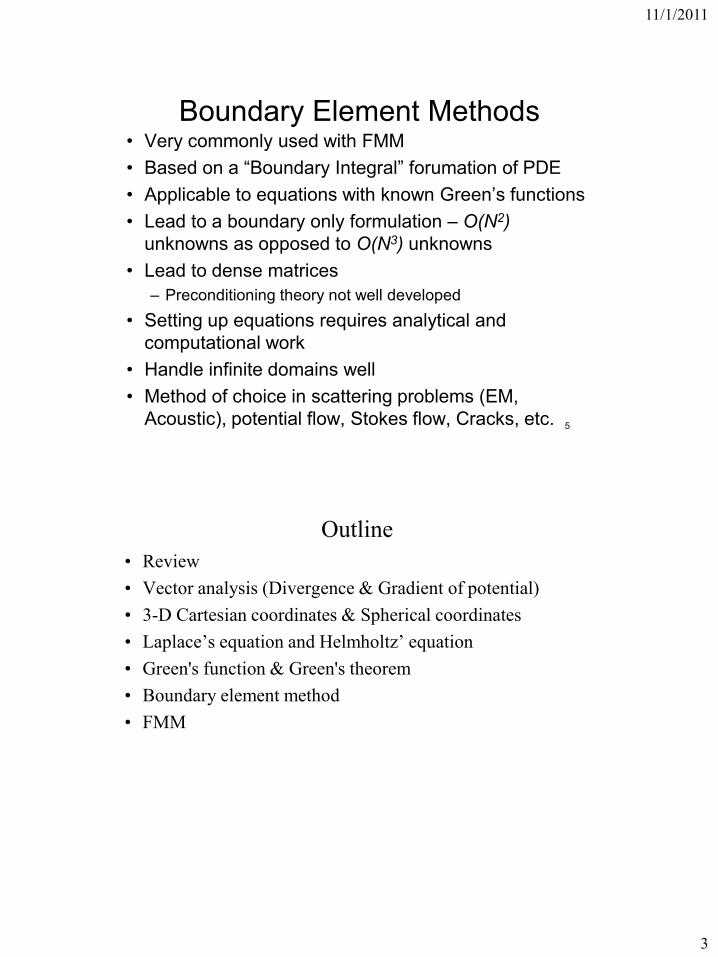
Boundary Element Methods • Very commonly used with FMM
• Based on a “Boundary Integral” forumation of PDE
• Applicable to equations with known Green’s functions
• Lead to a boundary only formulation – O(N2)
unknowns as opposed to O(N3) unknowns
• Lead to dense matrices
– Preconditioning theory not well developed
• Setting up equations requires analytical and
computational work
• Handle infinite domains well
• Method of choice in scattering problems (EM,
Acoustic), potential flow, Stokes flow, Cracks, etc. 5
Outline
• Review
• Vector analysis (Divergence & Gradient of potential)
• 3-D Cartesian coordinates & Spherical coordinates
• Laplace’s equation and Helmholtz’ equation
• Green's function & Green's theorem
• Boundary element method
• FMM

11/1/2011
4
Gauss Divergence theorem
• In practice we can write
Integral Definitions of div, grad and curl
Elemental volume
with surface S
τ 0
ΔS
τ 0
ΔS
τ 0
ΔS
1lim dS
τ
1lim . dS
τ
1lim dS
τ
n
D D n
D D n
n
dS
D=D(r), = (r)

11/1/2011
5
Green’s formula
Laplace’s equation

11/1/2011
6
Helmholtz equation
•
• Discretize surface S into triangles
• Discretize`

11/1/2011
7
Green’s formula • Recall that the impulse-response is sufficient to characterize
a linear system
• Solution to arbitrary forcing constructed via convolution
• For a linear boundary value problem we can likewise use
the solution to a delta-function forcing to solve it.
• Fluid flow, steady-state heat transfer, gravitational
potential, etc. can be expressed in terms of Laplace’s
equation
• Solution to delta function forcing, without boundaries, is
called free-space Green’s function
Boundary Element Methods
• Boundary conditions provide value of j or qj
• Becomes a linear system to solve for the other

11/1/2011
8
Accelerate via FMM

11/1/2011
9
Example 2: Boundary element
method
V
S
n
2
1

11/1/2011
10
Boundary element method(2)
Surface discretization:
System to solve:
Use iterative methods with fast matrix-vector multiplier:
Non-FMM’able, but sparse FMM’able, dense
Helmholtz equation Performance tests
Mesh: 249856 vertices/497664 elements
kD=29, Neumann problem kD=144, Robin problem
(impedance, sigma=1)
(some other scattering problems were solved)

11/1/2011
11
FMM & Fluid Mechanics • Basic Equations
1 2
n
Helmholtz Decomposition
• Key to integral equation and particle methods

11/1/2011
12
Potential Flow
• Knowledge of the potential is sufficient to compute velocity and pressure
• Need a fast solver for the Laplace equation
• Applications – panel methods for subsonic flow, water waves, bubble dynamics, …
Crum, 1979
Boschitsch et al, 1999
© Gumerov & Duraiswami, 2003
BEM/FMM Solution Laplace’s Equation
• Jaswon/Symm (60s) Hess & Smith (70s),
• Korsmeyer et al 1993, Epton & Dembart 1998, Boschitsch & Epstein 1999
Lohse, 2002

11/1/2011
13
Stokes Flow
• Green’s function (Ladyzhenskaya 1969, Pozrikidis 1992)
• Integral equation formulation
• Stokes flow simulations remain a very important area of research
• MEMS, bio-fluids, emulsions, etc.
• BEM formulations (Tran-Cong & Phan-Thien 1989, Pozrikidis 1992)
• FMM (Kropinski 2000 (2D), Power 2000 (3D))
Motion of spermatozoa
Cummins et al 1988
Cherax quadricarinatus.
MEMS force calculations
(Aluru & White, 1998
Rotational Flows and VEM • For rotational flows
Vorticity released at boundary layer or trailing edge and
advected with the flow
Simulated with vortex particles
Especially useful where flow is mostly irrotational
Fast calculation of Biot-Savart integrals
(x1,y1,z1)
(x2,y2,z2)
G nl
Evaluation
point
x
(where y is the
mid point of the
filament)
(circulation
strength)
(Far field)

11/1/2011
14
Vorticity formulations of NSE
• Problems with boundary conditions for this equation (see e.g., Gresho, 1991) Divergence free and curl-free components are linked only by boundary
conditions
Splitting is invalid unless potentials are consistent on boundary
• Recently resolved by using the generalized Helmholtz decomposition (Kempka et al, 1997; Ingber & Kempka, 2001)
• This formulation uses a kinematically consistent Helmholtz decomposition in terms of boundary integrals
• When widely adopted will need use of boundary integrals, and hence the FMM Preliminary results in Ingber & Kempka, 2001
Generalized Helmholtz Decomposition • Helmholtz decomposition leaves too many
degrees of freedom
• Way to achieve decomposition valid on boundary and in domain, with consistent values is to use the GHD
• D is the domain dilatation (zero for incompressible flow)
• Requires solution of a boundary integral equation as part of the solution => role for the FMM in such formulations