Three Essential ConceptsIn Wireless Audio.

© RF Venue, Inc., 2015

2www.RFvenue.com

Concept One:Signal-to-Noise Ratio

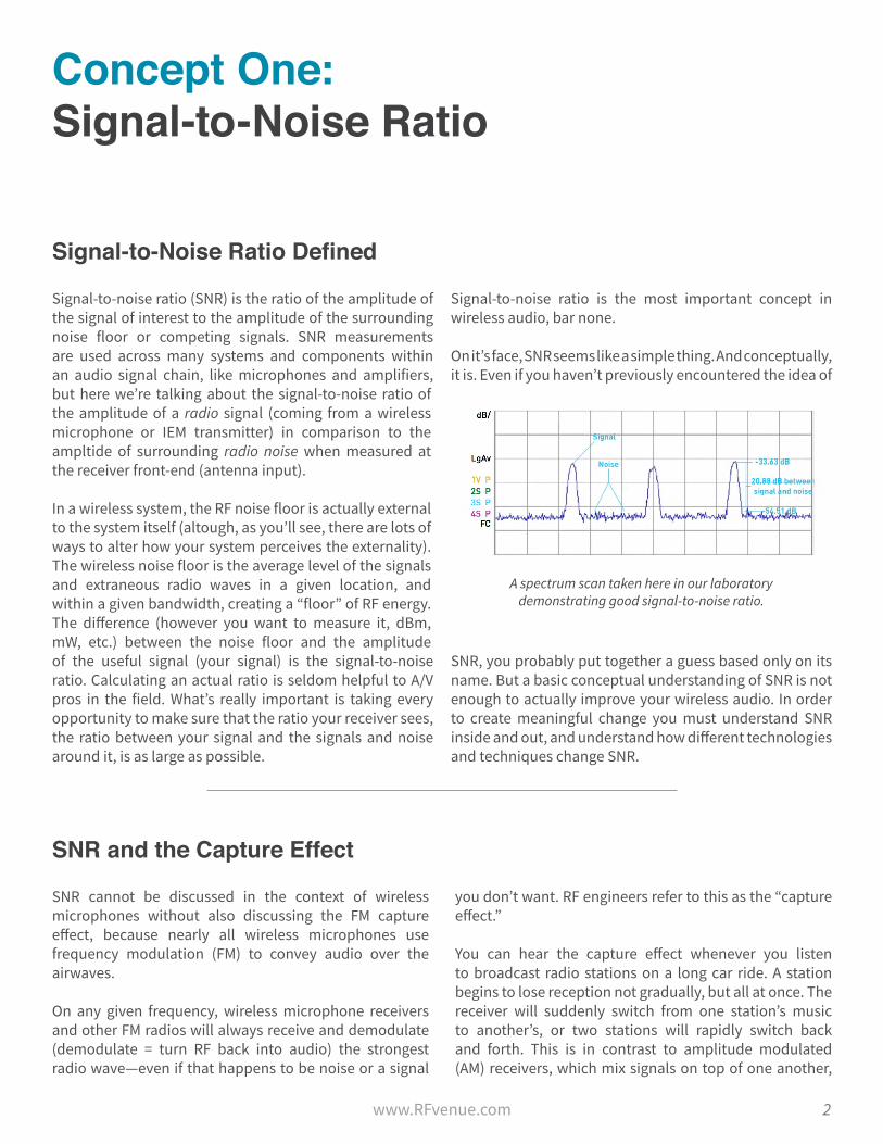
Signal-to-noise ratio (SNR) is the ratio of the amplitude of the signal of interest to the amplitude of the surrounding noise floor or competing signals. SNR measurements are used across many systems and components within an audio signal chain, like microphones and amplifiers, but here we’re talking about the signal-to-noise ratio of the amplitude of a radio signal (coming from a wireless microphone or IEM transmitter) in comparison to the ampltide of surrounding radio noise when measured at the receiver front-end (antenna input).

In a wireless system, the RF noise floor is actually external to the system itself (altough, as you’ll see, there are lots of ways to alter how your system perceives the externality).The wireless noise floor is the average level of the signals and extraneous radio waves in a given location, and within a given bandwidth, creating a “floor” of RF energy. The difference (however you want to measure it, dBm, mW, etc.) between the noise floor and the amplitude of the useful signal (your signal) is the signal-to-noise ratio. Calculating an actual ratio is seldom helpful to A/V pros in the field. What’s really important is taking every opportunity to make sure that the ratio your receiver sees, the ratio between your signal and the signals and noise around it, is as large as possible.

Signal-to-noise ratio is the most important concept in wireless audio, bar none.

On it’s face, SNR seems like a simple thing. And conceptually, it is. Even if you haven’t previously encountered the idea of

SNR, you probably put together a guess based only on its name. But a basic conceptual understanding of SNR is not enough to actually improve your wireless audio. In order to create meaningful change you must understand SNR inside and out, and understand how different technologies and techniques change SNR.

Signal-to-Noise Ratio Defined

SNR cannot be discussed in the context of wireless microphones without also discussing the FM capture effect, because nearly all wireless microphones use frequency modulation (FM) to convey audio over the airwaves.

On any given frequency, wireless microphone receivers and other FM radios will always receive and demodulate (demodulate = turn RF back into audio) the strongest radio wave—even if that happens to be noise or a signal

you don’t want. RF engineers refer to this as the “capture effect.”

You can hear the capture effect whenever you listen to broadcast radio stations on a long car ride. A station begins to lose reception not gradually, but all at once. The receiver will suddenly switch from one station’s music to another’s, or two stations will rapidly switch back and forth. This is in contrast to amplitude modulated (AM) receivers, which mix signals on top of one another,

SNR and the Capture Effect

A spectrum scan taken here in our laboratorydemonstrating good signal-to-noise ratio.

3www.RFvenue.com

resulting in two signals audible at the same time.

The capture effect occurs with very low difference between a signal of interest and a competing FM signal.

This difference depends on the receiver type and quality, but a rule of thumb is that 3-4 dB is needed between two signals for the receiver to demodulate one instead of the other. Sometimes manufacturers will publish a “capture ratio” specification in addition to a sensitivity and signal-to-noise ratio spec.

Here’s the take home point about SNR and the capture effect: In areas rich with competing FM signals, an FM receiver’s performance is either pass or fail, rather than stronger or weaker, because the signal of interest will either be heard or lost as the receiver locks on to one signal, or some of the energy of the competing transmitter leaks into the demodulation process (causing static) as the ratio between signal amplitudes changes. A difference of just a few dB—that is, just a slightly better signal-to-noise ratio—can be the difference between reception or interference.

An illustration of the capture effect. Signal A would be received and signal B would be completely suppressed, even though they are on

the same frequency.

SNR and the Capture Effect (contd.)

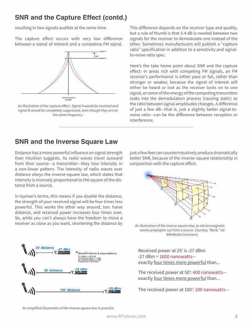
SNR and the Inverse Square LawDistance has a more powerful influence on signal strength than intuition suggests. As radio waves travel outward from their source—a transmitter—they lose intensity in a non-linear pattern. The intensity of radio waves over distance obeys the inverse-square law, which states that intensity is inversely proportional to the square of the dis-tance from a source.

In layman’s terms, this means if you double the distance, the strength of your received signal will be four times less powerful. This works the other way around, too: halve distance, and received power increases four times over. So, while you can’t always have the freedom to move a receiver as close as you want, shortening the distance by

just a few feet can counterintuitively produce dramatically better SNR, because of the inverse-square relationship in conjunction with the capture effect.

An illustration of the inverse square law, as electromagneticwaves propogate out from a source. Courtesy “Borb,” via

WikiMedia Commons.

An simplified illustration of the inverse square law in practice.

Received power at 25’ is -27 dBm: -27 dBm = 1600 nanowatts—exactly four times more powerful than...

The received power at 50’: 400 nanowatts—exactly four times more powerful than...

The received power at 100’: 100 nanowatts—

4www.RFvenue.com

SNR and the Physical Layer

Signal-to-noise ratio is the most important concept in wireless audio because positively changing SNR gives the most pronounced improvement in signal quality, and it is the variable that the end-user has the most control of.

There is never a situation where a lower SNR provides bet-ter performance over a higher SNR, all other factors being equal. Never.

And yet, for all it’s importance, because the majority “noise” part of wireless signal-to-noise ratio usually exists outside of the electrical audio and RF system, manipulating SNR is something that must—and in fact can only—be done by manipulating what network engineers refer to as the “physical layer.”

The terminology “physical layer” is inherited from the OSI model of network architecture. It is usually used to describe the way, and the materials, in which raw bits of information are transported from one place to another in a computer network.

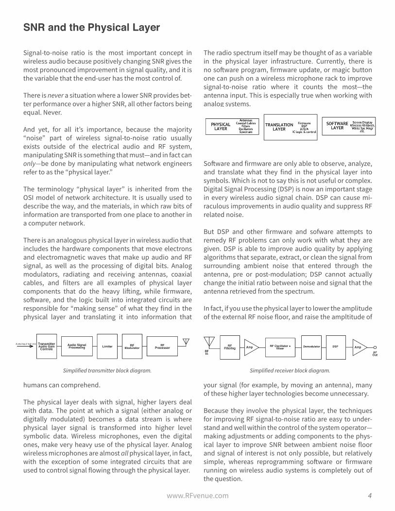
There is an analogous physical layer in wireless audio that includes the hardware components that move electrons and electromagnetic waves that make up audio and RF signal, as well as the processing of digital bits. Analog modulators, radiating and receiving antennas, coaxial cables, and filters are all examples of physical layer components that do the heavy lifting, while firmware, software, and the logic built into integrated circuits are responsible for “making sense” of what they find in the physical layer and translating it into information that

humans can comprehend.

The physical layer deals with signal, higher layers deal with data. The point at which a signal (either analog or digitally modulated) becomes a data stream is where physical layer signal is transformed into higher level symbolic data. Wireless microphones, even the digital ones, make very heavy use of the physical layer. Analog wireless microphones are almost all physical layer, in fact, with the exception of some integrated circuits that are used to control signal flowing through the physical layer.

The radio spectrum itself may be thought of as a variable in the physical layer infrastructure. Currently, there is no software program, firmware update, or magic button one can push on a wireless microphone rack to improve signal-to-noise ratio where it counts the most—the antenna input. This is especially true when working with analog systems.

Software and firmware are only able to observe, analyze, and translate what they find in the physical layer into symbols. Which is not to say this is not useful or complex. Digital Signal Processing (DSP) is now an important stage in every wireless audio signal chain. DSP can cause mi-raculous improvements in audio quality and suppress RF related noise.

But DSP and other firmware and sofware attempts to remedy RF problems can only work with what they are given. DSP is able to improve audio quality by applying algorithms that separate, extract, or clean the signal from surrounding ambient noise that entered through the antenna, pre or post-modulation; DSP cannot actually change the initial ratio between noise and signal that the antenna retrieved from the spectrum.

In fact, if you use the physical layer to lower the amplitude of the external RF noise floor, and raise the ampltitude of

your signal (for example, by moving an antenna), many of these higher layer technologies become unnecessary.

Because they involve the physical layer, the techniques for improving RF signal-to-noise ratio are easy to under-stand and well within the control of the system operator—making adjustments or adding components to the phys-ical layer to improve SNR between ambient noise floor and signal of interest is not only possible, but relatively simple, whereas reprogramming software or firmware running on wireless audio systems is completely out of the question.

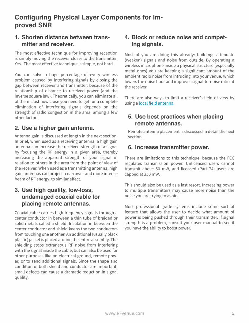
Simplified transmitter block diagram. Simplified receiver block diagram.

5www.RFvenue.com

2. Use a higher gain antenna.

3. Use high quality, low-loss, undamaged coaxial cable for placing remote antennas.

4. Block or reduce noise and compet-ing signals.

5. Use best practices when placing remote antennas.

6. Increase transmitter power.

Remote antenna placement is discussed in detail the next section.

1. Shorten distance between trans-mitter and receiver.

Configuring Physical Layer Components for Im-proved SNR

The most effective technique for improving reception is simply moving the receiver closer to the transmitter. Yes. The most effective technique is simple, not hard.

You can solve a huge percentage of every wireless problem caused by interfering signals by closing the gap between receiver and transmitter, because of the relationship of distance to received power (and the inverse square law). Theoretically, you can eliminate all of them. Just how close you need to get for a complete elimination of interfering signals depends on the strength of radio congestion in the area, among a few other factors.

Antenna gain is discussed at length in the next section. In brief, when used as a receiving antenna, a high gain antenna can increase the received strength of a signal by focusing the RF energy in a given area, thereby increasing the apparent strength of your signal in relation to others in the area from the point of view of the receiver. When used as a transmitting antenna, high gain antennas can project a narrower and more intense beam of RF energy, to similar effect.

Coaxial cable carries high frequency signals through a center conductor in between a thin tube of braided or solid metals called a shield. Insulation in between the center conductor and shield keeps the two conductors from touching one another. An additional (usually black plastic) jacket is placed around the entire assembly. The shielding stops extraneous RF noise from interfering with the signal inside the cable, but can also be used for other purposes like an electrical ground, remote pow-er, or to send additional signals. Since the shape and condition of both shield and conductor are important, small defects can cause a dramatic reduction in signal quality.

Most of you are doing this already: buildings attenuate (weaken) signals and noise from outside. By operating a wireless microphone inside a physical structure (especially metal ones) you are keeping a significant amount of the ambient radio noise from intruding into your venue, which lowers the noise floor and improves signal-to-noise ratio at the receiver.

There are also ways to limit a receiver’s field of view by using a local field antenna.

There are limitations to this technique, because the FCC regulates transmission power. Unlicensed users cannot transmit above 50 mW, and licensed (Part 74) users are capped at 250 mW.

This should also be used as a last resort. Increasing power to multiple transmitters may cause more noise than the noise you are trying to avoid.

Most professional grade systems include some sort of feature that allows the user to decide what amount of power is being pushed through their transmitter. If signal strength is a problem, consult your user manual to see if you have the ability to boost power.

6www.RFvenue.com

Concept Two:Antenna Gain

Antenna Gain DefinedAntenna gain is a mathematical description of the way a given antenna focuses or projects electromagnetic energy into physical space.

Gain is sometimes informally referred to as the “coverage pattern,” but gain is more than just a coverage pattern.

The formal definition of antenna gain is antenna efficiency plus directivity, which is measured in decibels.

Antenna efficiency is the proportion of electrical energy that a given antenna is able to convert into electromagnetic energy (radio waves), or reciprocally, the proportion of electromagnetic energy an antenna is able to convert into electrical energy.

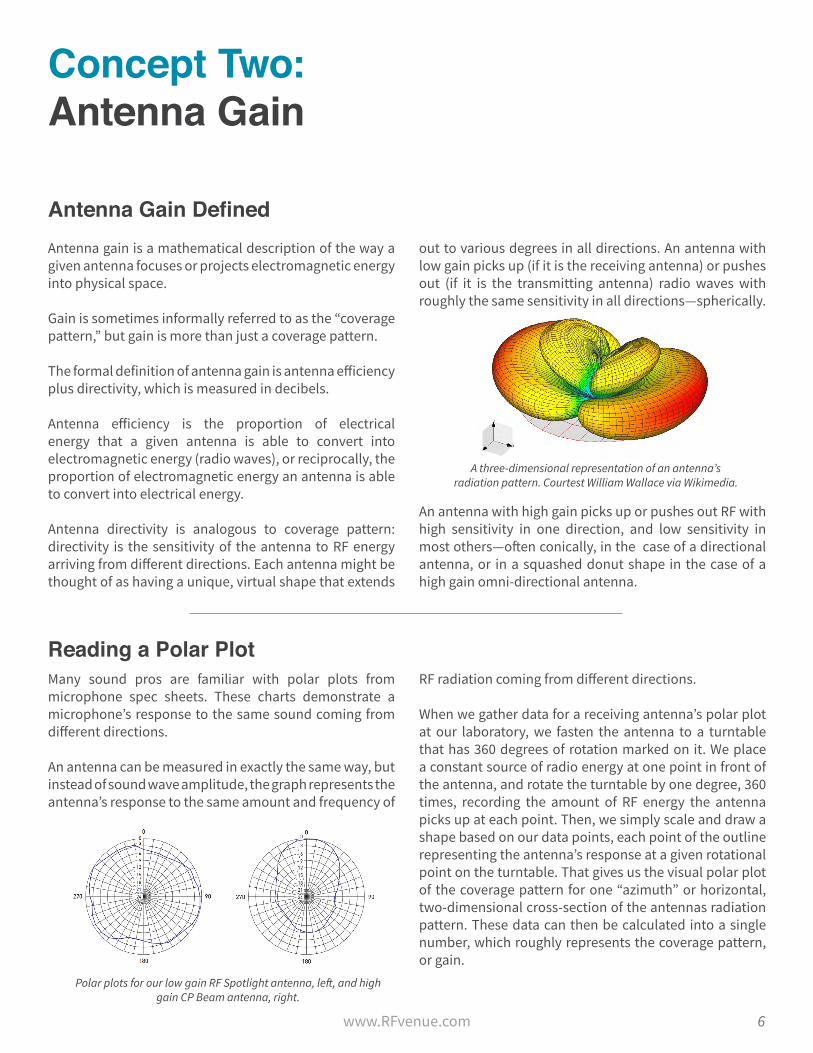
Antenna directivity is analogous to coverage pattern: directivity is the sensitivity of the antenna to RF energy arriving from different directions. Each antenna might be thought of as having a unique, virtual shape that extends

out to various degrees in all directions. An antenna with low gain picks up (if it is the receiving antenna) or pushes out (if it is the transmitting antenna) radio waves with roughly the same sensitivity in all directions—spherically.

An antenna with high gain picks up or pushes out RF with high sensitivity in one direction, and low sensitivity in most others—often conically, in the case of a directional antenna, or in a squashed donut shape in the case of a high gain omni-directional antenna.

Reading a Polar PlotMany sound pros are familiar with polar plots from microphone spec sheets. These charts demonstrate a microphone’s response to the same sound coming from different directions.

An antenna can be measured in exactly the same way, but instead of sound wave amplitude, the graph represents the antenna’s response to the same amount and frequency of

RF radiation coming from different directions.

When we gather data for a receiving antenna’s polar plot at our laboratory, we fasten the antenna to a turntable that has 360 degrees of rotation marked on it. We place a constant source of radio energy at one point in front of the antenna, and rotate the turntable by one degree, 360 times, recording the amount of RF energy the antenna picks up at each point. Then, we simply scale and draw a shape based on our data points, each point of the outline representing the antenna’s response at a given rotational point on the turntable. That gives us the visual polar plot of the coverage pattern for one “azimuth” or horizontal, two-dimensional cross-section of the antennas radiation pattern. These data can then be calculated into a single number, which roughly represents the coverage pattern, or gain.

A three-dimensional representation of an antenna’sradiation pattern. Courtest William Wallace via Wikimedia.

Polar plots for our low gain RF Spotlight antenna, left, and high gain CP Beam antenna, right.

7www.RFvenue.com

Antenna Gain Changes SNRBecause antennas are able to shape and concentrate the fields of RF energy that travel between transmitter and receiver, they are one of the most powerful ways to influence SNR.

A transmitter using a high gain antenna pointed at a receiver also outfitted with a high gain antenna will strengthen the signal of interest while lowering the noise floor, because, with the antenna pointed at one another, it’s like a telescope pointed at a telescope. In wireless audio applications, a user usually only gets one high gain antenna, either transmit or receive, because the talent is always using a handheld or beltpack for mics or IEMs that is outfitted with an omni-directional antenna.

If two low gain antennas are used, one for transmit and one for receive, the receive antenna will only see the transmitters signal diffusely against the background noise of ambient radiation they collect from all directions.

If there is a source of interference that has a known, physical source, like an LED wall, competing stage (as at a music festival), or bad circuit breaker, a high gain

directional antenna can be positioned in such a way as to place the performer inside the coverage area of the antenna, and the source of interference on the outside, or “off-axis”, effectively increasing SNR by attenuating the source of interference and increasing the apparent signal strength.

Counterintuitively, low gain antennas can also be used to increase SNR, because of the inverse-square law. If you can get a low gain antenna very close to a source, the signals arriving from transmitters near the antenna will appear to be strong to the receiver, while competing signals and noise from farther away will be low in ampltitude by comparison.

We designed the Spotlight antenna around this concept. The Spotlight has a very unique coverage pattern, that of a hemisphere, and very low gain. It is mounted in a flat, 7mm disc, and is actually placed on the floor or underneath a stage directly underneath or nearby performers. In this way, it tends to pick up signals directly above it, while attenuating competing signals arriving from the far horizon.

We retrieved a superb visual demonstration of the Spotlight’s benefits while working with The Public Theater in New York City on their 2015 productions of the long-running Shakespeare in the Park, which is produced in an outdoor, open air theater in the heart of Central Park in Manhattan. Two Spotlights were mounted underneath the stage and, when compared with helicals also in use, dramatically increased the number of useable channels by deafening nearby DTV transmitters—transforming a 6 MHz channel’s SNR from completely unusable to the baseline noise-floor.

Two helical antenna deployed to avoid near-fieldRFI from a troublesome video wall.

Spectrum trace overlay during Shakespeare in the Park,demonstrating improved SNR through antenna pattern.

GREEN = Helical antenna / RED = Spotlight antenna

8www.RFvenue.com

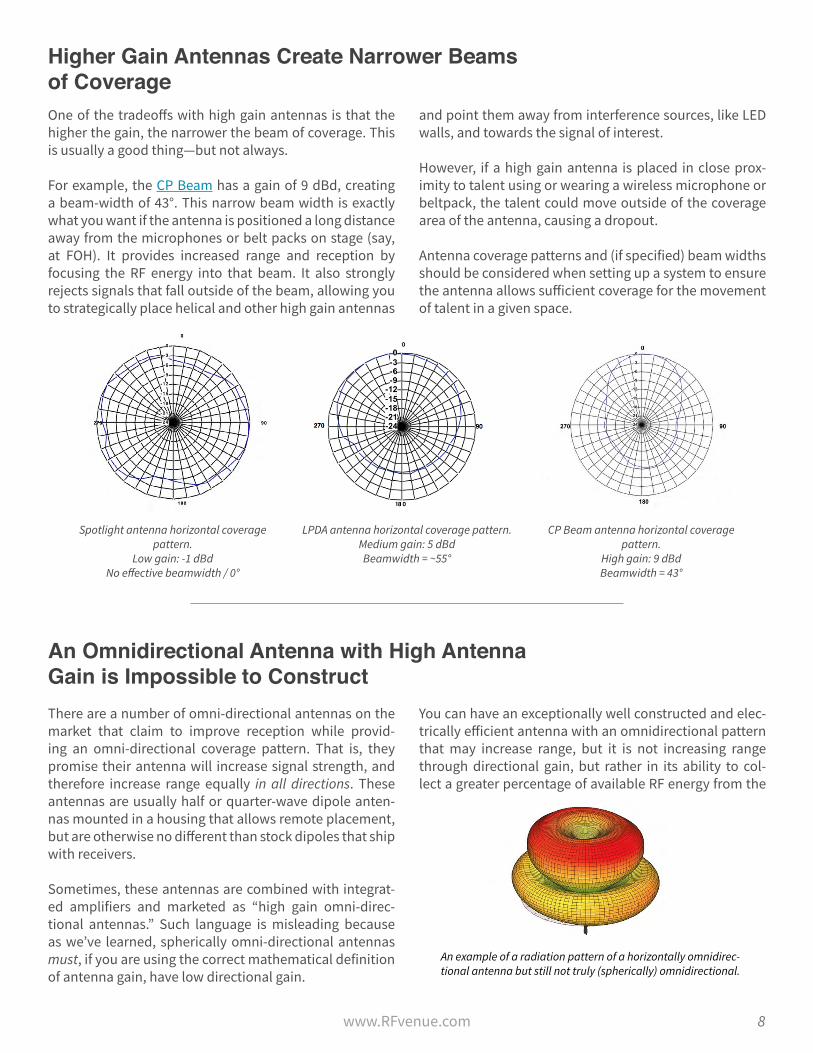
Higher Gain Antennas Create Narrower Beams of CoverageOne of the tradeoffs with high gain antennas is that the higher the gain, the narrower the beam of coverage. This is usually a good thing—but not always.

For example, the CP Beam has a gain of 9 dBd, creating a beam-width of 43°. This narrow beam width is exactly what you want if the antenna is positioned a long distance away from the microphones or belt packs on stage (say, at FOH). It provides increased range and reception by focusing the RF energy into that beam. It also strongly rejects signals that fall outside of the beam, allowing you to strategically place helical and other high gain antennas

and point them away from interference sources, like LED walls, and towards the signal of interest.

However, if a high gain antenna is placed in close prox-imity to talent using or wearing a wireless microphone or beltpack, the talent could move outside of the coverage area of the antenna, causing a dropout.

Antenna coverage patterns and (if specified) beam widths should be considered when setting up a system to ensure the antenna allows sufficient coverage for the movement of talent in a given space.

Spotlight antenna horizontal coverage pattern.

Low gain: -1 dBdNo effective beamwidth / 0°

LPDA antenna horizontal coverage pattern.Medium gain: 5 dBdBeamwidth = ~55°

CP Beam antenna horizontal coverage pattern.

High gain: 9 dBdBeamwidth = 43°

An Omnidirectional Antenna with High Antenna Gain is Impossible to ConstructThere are a number of omni-directional antennas on the market that claim to improve reception while provid-ing an omni-directional coverage pattern. That is, they promise their antenna will increase signal strength, and therefore increase range equally in all directions. These antennas are usually half or quarter-wave dipole anten-nas mounted in a housing that allows remote placement, but are otherwise no different than stock dipoles that ship with receivers.

Sometimes, these antennas are combined with integrat-ed amplifiers and marketed as “high gain omni-direc-tional antennas.” Such language is misleading because as we’ve learned, spherically omni-directional antennas must, if you are using the correct mathematical definition of antenna gain, have low directional gain.

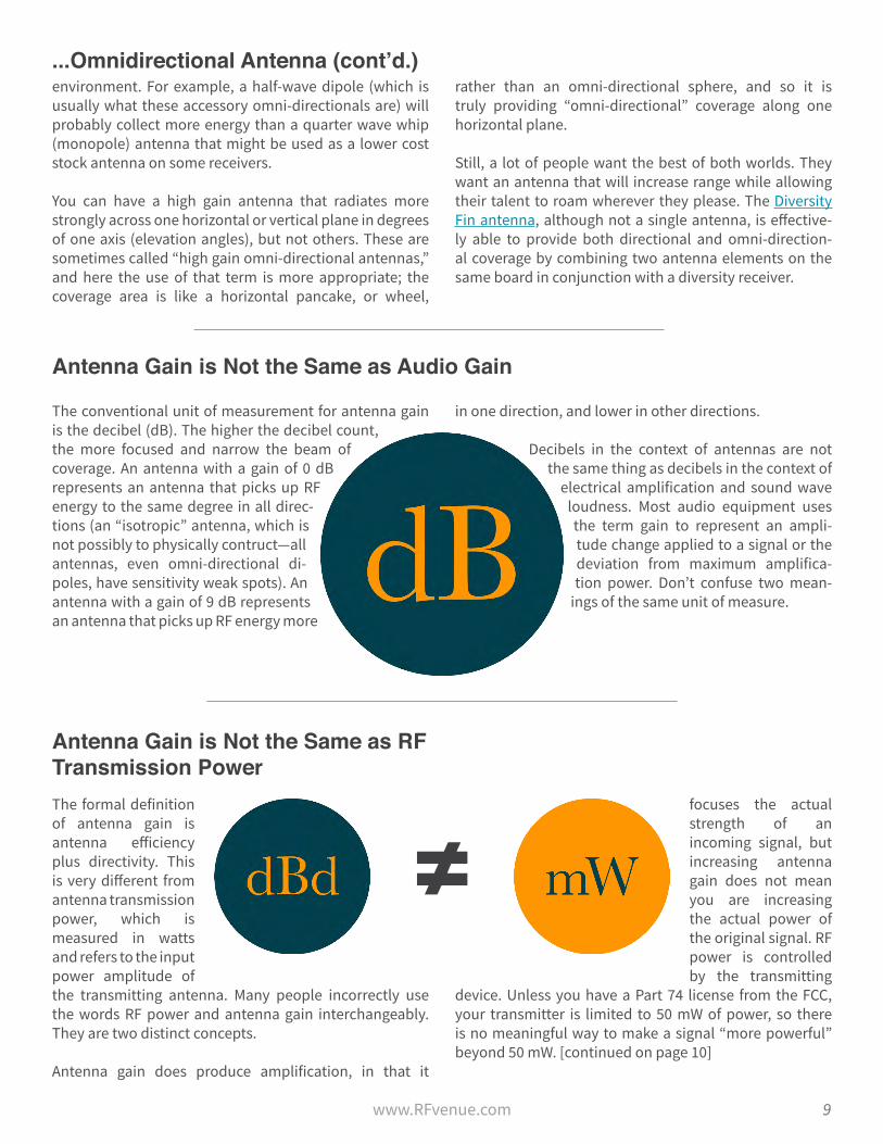
You can have an exceptionally well constructed and elec-trically efficient antenna with an omnidirectional pattern that may increase range, but it is not increasing range through directional gain, but rather in its ability to col-lect a greater percentage of available RF energy from the

An example of a radiation pattern of a horizontally omnidirec-tional antenna but still not truly (spherically) omnidirectional.

9www.RFvenue.com

environment. For example, a half-wave dipole (which is usually what these accessory omni-directionals are) will probably collect more energy than a quarter wave whip (monopole) antenna that might be used as a lower cost stock antenna on some receivers.

You can have a high gain antenna that radiates more strongly across one horizontal or vertical plane in degrees of one axis (elevation angles), but not others. These are sometimes called “high gain omni-directional antennas,” and here the use of that term is more appropriate; the coverage area is like a horizontal pancake, or wheel,

rather than an omni-directional sphere, and so it is truly providing “omni-directional” coverage along one horizontal plane.

Still, a lot of people want the best of both worlds. They want an antenna that will increase range while allowing their talent to roam wherever they please. The Diversity Fin antenna, although not a single antenna, is effective-ly able to provide both directional and omni-direction-al coverage by combining two antenna elements on the same board in conjunction with a diversity receiver.

...Omnidirectional Antenna (cont’d.)

Antenna Gain is Not the Same as Audio Gain

The conventional unit of measurement for antenna gain is the decibel (dB). The higher the decibel count, the more focused and narrow the beam of coverage. An antenna with a gain of 0 dB represents an antenna that picks up RF energy to the same degree in all direc-tions (an “isotropic” antenna, which is not possibly to physically contruct—all antennas, even omni-directional di-poles, have sensitivity weak spots). An antenna with a gain of 9 dB represents an antenna that picks up RF energy more

in one direction, and lower in other directions.

Decibels in the context of antennas are not the same thing as decibels in the context of

electrical amplification and sound wave loudness. Most audio equipment uses the term gain to represent an ampli-tude change applied to a signal or the deviation from maximum amplifica-tion power. Don’t confuse two mean-

ings of the same unit of measure.

Antenna Gain is Not the Same as RF Transmission PowerThe formal definition of antenna gain is antenna efficiency plus directivity. This is very different from antenna transmission power, which is measured in watts and refers to the input power amplitude of the transmitting antenna. Many people incorrectly use the words RF power and antenna gain interchangeably. They are two distinct concepts.

Antenna gain does produce amplification, in that it

focuses the actual strength of an incoming signal, but increasing antenna gain does not mean you are increasing the actual power of the original signal. RF power is controlled by the transmitting

device. Unless you have a Part 74 license from the FCC, your transmitter is limited to 50 mW of power, so there is no meaningful way to make a signal “more powerful” beyond 50 mW. [continued on page 10]

≠

10www.RFvenue.com

Antenna Gain is Not the Same as RF Transmission Power (cont’d.)There are a number of pre-amplified antennas on the market which are marketed as “active” antennas. These devices do not increase antenna gain, and they do not increase transmission power. They boost the electrical signal on a long, lossy feed line. If you have a weak signal and a low noise floor, some pre- amplification can be useful. If there is a high noise floor, which is more common, then preamplifiers also amplify the noise. This can

produce an overload condition at the receiver in certain instances. Preamplifiers, if used incorrectly can introduce unwanted noise into the system, overload the front end of the receiver, and increase intermodulation products. We typically do not recommend powered antennas for general use because managing gain structure is required to avoid unwanted side effects.

BUT... Antenna Gain Does Influence Effective Radiated Power (ERP)Antenna Gain Must be Understood as one of many links in the physical layer signal chain

In both transmit and receive applications, antenna gain influences the effective amplitude of a signal significantly, but it is only one of many physical layer components that do so.

Amplifiers, cables, and connectors also influence the amount of “effective” electromagnetic power that is radiated out into space, or, the amount of power that a receiver is able to recover from the airwaves.

You may know your antenna gain, your transmitter power, as well as the length of coaxial cable you are using to remote your antenna and how many dB it loses per foot,

but if you want to know the true amount of energy that is being transmitted or received, you should know how to calculate ERP, or Effective Radiated Power.

ERP is really quite simple. It is the output power of the

transmitter, plus the gain of the antenna, minus the attenuation and losses incurred by cable runs and connectors in-between the transmitter and antenna.

The circuitry and amplifiers inside a transmitter push the signal up to a certain level to the output connection. If you were using an IEM transmitter at 50 mW with no antenna attached, the output would be approximately 50 mW.

All coaxial cable attenuates (weakens) signal. The amount of attenuation depends on 1) transmit frequency, 2) the type of coax used, and 3) the length of the cable. All of these variables are predictable. Loss from connectors should be minimal if everything is screwed in tight, but there will always be a little bit.

Antennas can be thought of as lenses, focusing the energy coming from the transmitter down into a narrow field, which intensifies its effective radiated power as it travels out into space. Antennas with high gain are like telephoto lenses. They increase ERP. Antennas with low gain are like

11www.RFvenue.com

normal lenses. They create little to no increase in ERP.An antenna’s effect on ERP can be quite dramatic. For example, if you were to plug a 9 dBd CP Beam directly into the output of a 50 mW IEM transmitter, the ERP would be magically transformed into 390 mW of power radiated at the source (the antenna) in a concentrated beam of RF.

In the UHF broadcast band, between 470-698 MHz, both unlicensed and licensed (Part 74) users are allowed to attach antennas of reasonable gain to their transmitters. As long as the power at the antenna input does not exceed 50 mW unlicensed/250 mW licensed, there are no hard and fast rules on ERP emission limits. However,

the golden rule is always to protect licensed users or, for 74 licensees, protect TV stations. If you do use some sort of configuration that creates interference to a licensed service, the fault is yours.

At 2.4 GHz, output power is capped at 1 watt, and ERP is capped at 4 watts. That means you need to be careful attaching high gain antennas to 2.4 GHz transmitters.

ERP (cont’d.)

Concept Three:Electromagnetic Spectrum& Spectrum ManagementRadio Spectrum DefinedThe “signals” we have talked about in our previous discussion on signal-to-noise ratio are made of a type of oscillating, or repeating, energy known as electromagnetic radiation.

For the sake of simplicity, let’s describe electromagnetic radiation as patterns of energy that repeat and self-propagate outward through space.

Electromagnetic radiation can oscillate across a very wide range of frequencies.

“Frequency” means the number of times the pattern of electromagnetic energy repeats in one second. The unit of measure, as with mechanical sound waves (another form of oscillating energy) is the Hertz. An electromagnetic wave of 1 Hz returns to its original phase after one second. An electromagnetic wave of 500 Hz repeats its oscillation five hundred times in one second. Electromagnetic radiation can be very low in frequency, to very, very high, or anywhere in-between.

These frequencies of radiation, all of them, collectively, are known as the electromagnetic spectrum.

The characteristics of electromagnetic radiation vary widely depending on frequency. Light is a form of EM radiation, as are X-rays and gamma rays. They vary so much, in fact, that the physical rules for low frequency radiation, like radio waves, are not the same as they are for high frequency radiation, like light.

Traditionally, the so called “radio” spectrum is that portion of the electromagnetic spectrum which can be modulated to carry information. Radio modulation is the process by which audio signals in electrical current are transformed into audio information-carrying radio waves.

In the past, separating the radio spectrum from the larger electromagnetic spectrum was much easier, since modu-lation was restricted by the technical limitations of prim-itive analog transmitters and receivers, and the raw fre-quencies their oscillators were capable of generating. As recently as the pre-war period... [continued on page 13]....

12www.RFvenue.com

An attempt to visually display how little spectrum is available for wireless audio devices in the context of other legal allocations, and the entire electromagnetic spectrum at large.

13www.RFvenue.com

radios operating in the MHz range (millions of oscillations per second) were inconceivably high, and hence the radio spectrum at that time was much smaller.

As technology has progressed, more and more of the electromagnetic spectrum has been unlocked as an information carrying medium. We use radios that operate in the gigahertz range (GHz, billions of oscillations per second) every day. WiFi, for example, typically uses spectrum between 2.4 and 2.5 GHz. And scientists are hard at work developing technologies that can carry information efficiently at frequencies in the terahertz range (trillions of cycles per second/THz), although those technologies have yet to reach mass markets.

Hence, we are left with a useful but tentative definition of the radio spectrum by the ITU as being between 8.3 kHz and 3000 GHz.

Wireless microphones operate within very small slices of this vast radio spectrum.

The majority of wireless audio devices operate between 400-800 MHz, depending on the country of operation. There are also wireless audio devices that operate in other frequencies bands, like 900 MHz, 2.4 GHz, and 5.8 GHz.

The reasons why most wireless audio devices operate in UHF (300-3000 MHz) band are a mixture of the desirable propagation characteristics of radio waves of those frequencies, the characteristics of antennas, government regulation, market forces, and chance.

There is no hard and fast ‘real’ rule, based in physics, that prohibits a wireless microphone from utilizing frequencies above or below 300 and 3000 MHz, and sounding just as good. In fact, we have seen the introduction of new technologies that place devices as low as 72 MHz, and as high as 5.8 GHz, in recent years. We should expect future equipment to utilize frequencies significantly above and below the current standard range of broadcast band UHF.

Radio Spectrum Defined (contd.)

Frequency, Wavelength, and TimeThere is an important relationship between frequency of oscillation, the distance traveled by a wave in one oscillation, and time.

Since all forms of electromagnetic radiation travel through a vacuum at exactly the speed of light, we have a convenient mathematical constant with which to measure and quantify the characteristics of EM energies.

Any given frequency will have a corresponding wavelength, and vice versa, because all forms of EM radiation, no matter their frequency, travel at the same speed (distance traveled over time) through a vacuum: the speed of light.

Since light travels at about 300,000,000 meters per second in a vacuum (and we ignore that the speed of EM waves changes in other mediums) we can derive any frequency’s wavelength from its frequency, and any wavelength’s fre-quency from its wavelength. For the MHz range (millions of oscillations per second) that gives us a handy formula.

Wavelength λ in meters = 300 / Frequency in MHz

If we know that the frequency of a transmitter’s signal is 550 MHz, for example, then we also known that signal’s wavelength. Here the wavelength is 300 divided 550, or 0.5454 meters.

14www.RFvenue.com

Frequency, Wavelength, and Time (contd.)But say we only knew the wavelength, and wanted to find the frequency, we could rearrange the formula.

Frequency in MHz = 300 / 0.5454 meters

Which gives us about 550 MHz.

Understanding the basic characteristics and behaviors or electromagnetic waves is important to the wireless audio operator for a number of reasons.

Different frequencies have different propagation characteristics. Generally, the lower the frequency, the farther it can travel given the same transmission energy, and the greater ease it has passing through physical objects, like walls. Higher frequencies with shorter wavelengths usually travel through air less far than lower frequencies using the same amount of energy, and have greater difficulty penetrating physical objects.

Higher frequencies also attenuate, or lose strength/amplitude, to a much greater degree inside runs of coaxial cable than lower frequencies. These differences should be considered when a system in one or another range is

purchased. There are also practical cost reasons why UHF (~470-800 MHz) is a good frequency range to be in. As we calculated above, a wireless microphone transmitter operating on a frequency of 550 MHz has a full wavelength of 0.54 meters, or 21 inches. A good antenna usually has one dimension that is equal to the full, half, or quarter harmonic dimensions of the wavelength. At UHF frequencies, the longest dimension of 1/4 wave dipole antennas is a manageable 5-7 inches, and 1/2 wave antennas are about a foot long. Analog components inside UHF transmitters and receivers are also more compact and less costly to make than equipment using lower frequencies. A VHF system operating at 216 MHz has a full wavelength of 55 inches! Which translates to a stock dipole or whip antenna that is over 13” long for a 1/4 wave, and 28” for a 1/2 wave. For the most part, equipment that uses sub UHF frequencies has bulkier antennas and accessories, and can also cost more too. In comparison, 2.4 GHz equipment can be manufactured at relatively lower cost because 2.4 GHz chips and components are ubiquitous from the data industry, and the antennas and physical layer components required for good performance are smaller: a 1/2 wave dipole at 2.4 GHz is only 2.5 inches!

Spectrum RegulationUnlike other forms of audiovisual communications, wireless is unique in that the medium its signal travels through is, for lack of a better word, public.

A radio wave spreads out in physical space. It is not safely confined inside a cable, or locked away in a hard drive. A radio wave spreads through other private and public spaces that you may or may not be affiliated with. Those radio waves are not isolated or inert; they interact with other RF equipment in other places. Sometimes, these interactions are good. Other times, they are bad. If they are bad, we usually call those interactions “interference.”

Only one signal can occupy one frequency in one location at one time. (Technically, there is no such thing as “one” frequency, because electromagnetic radiation exists on an infinitely varying spectrum, but signals generated by transmitters do have bandwidths, which are the total RF “footprint” or range of frequencies that a signal takes up on the spectrum.)

Because radio waves are a dynamic medium that create fields of energy around their source, and signals use bandwidth, spectrum is finite. That is, in one given area,

spectrum can be overused or congested. If there are two many radios generating too many signals that exceed the capacity of the spectrum in one area, radios will begin to interfere with one-another and the usefulness of the spectrum will diminish for all.

Because of these unique properties, many have made the argument that spectrum is a public natural resource. It is initially difficult to conceive of electromagnetic radiation as a natural resource like an aquifer or stands of timber because it isn’t something that can be seen or touched—but it most certainly is useful like a resource. It can be temporarily depleted by human overuse, like aquifers and forests, and is “natural” in that it is found naturally in the physical world, rather than being something that humankind has created.

A different but related analogy is thinking of electromagnetic spectrum as a public utility, like a road or water distribution system, which are engineered by humans, but can likewise be overused.

Which brings us to regulation. As a natural resource, spectrum must be managed to avoid

15www.RFvenue.com

Spectrum Regulation (contd)overuse. There is no clear-cut consensus on how to do that. Academics have discussed spectrum management policy for decades. The discipline combines economics, law, and engineering to debate optimum models for distributing spectrum in the most equitable and efficient way possible. Learning just a little bit about these theories helps us

understand why the rules we have are the way they are, and how and why we should follow them, or push to have them changed.

Although it may seem as if the federal government is far removed when we use wireless microphones and other audio devices, spectrum regulations have far reaching benefits and consequences for the wireless audio user. They regulate the frequencies we can use, where we can use them, our transmission power, ERP, carrier signal characteristics, and many other important constraints.

Currently, the regulation of spectrum in most developed countries is undergoing significant change at a blistering pace.

New technologies—notably cellular and data technologies from the mobile revolution—all require spectrum, and it just so happens that the spectrum wireless microphones

currently use—UHF—has many of the same benefits for smartphones as it does for wireless microphones and the digital television stations that are UHF incumbents.

Most countries, following the lead of the United States, UK, and Sweden (the former country the home of wire-less technology behemoth multinational Ericsson, in case you’re wondering why they made the list), have decided, not without controversy, that the spectrum currently used by wireless audio devices and over-the-air television stations would better serve society if those frequencies were allocated to mobile and broadband purposes.

The world is in the middle of a large and sustained effort to repurpose UHF spectrum from broadcasting, wireless audio, and a few other uses to spectrum that is regulated for private-sector cellular and data carriers.

In the United States, we experienced the iron fist of that transition when, with comparatively little warning, the 700 MHz range was auctioned off to mobile carriers in 2008, and wireless mics and broadcasters were swiftly evicted from that range.

In 2016, the first ever incentive auctions will begin the pro-cess of clearing the 600 MHz band of wireless audio devic-es and television broadcasters in lieu of mobile carriers. Future reallocations are almost inevitable.

Whatever your personal feelings on these government regulations, those feelings will not prevent future reallo-cations from happening. The industry has fought hard to keep as much UHF spectrum as possible for as long as pos-sible—but the odds are against us, and we should prepare sooner rather than later to adopt newer, more efficient radio technologies in both new and old frequency ranges.

The age of the mobile connectivity and its voracious spectrum appetite will not destroy wireless audio, but it will make it different.

Government regulation of electromagnetic spectrum is a complex and dynamic science and political art, as this excerpt from a visual-

ization of the United States’ allocations shows.

16www.RFvenue.com

Wireless Audio and Spectrum EfficiencyToday, most wireless microphones use analog wideband FM modulation to transmit audio in wireless form.

There’s a lot to unpack in that sentence.

An “analog” modulation of a radio wave changes frequency or amplitude in way that is directly related to the varying nature of the electrical signal that the modulation circuit is fed. The wave has no single value, but is in a state of constant variation.

“FM” stands for “frequency modulation.” In an analog FM system, an RF carrier wave varies its frequency in proportion to changes in an audio wave’s amplitude and frequency.

“Wideband” can mean different things, depending on who you ask. Electrical engineers might start talking about something called the “modulation index,” but for the purposes of this paper, in our industry “wideband” is generally used to refer to the bandwidth limitations that are imposed on FM transmitters. In the United States, the FCC regulates the deviation of the carrier wave of a wireless audio device to no more than 100 kHz above or below the center frequency, for a total allowed bandwidth of 200 kHz—although in practice a well made transmitter may use less bandwidth than 200 kHz.

By comparison, the two-way and public safety radio industries, which are also frequency modulated, were required to upgrade to “narrowband” transmitters in 2013 that use a carrier wave that consumes only 12.5 kHz.

Eventually, the FCC would like two-way radios to consume even less bandwidth—6.25 kHz.

The two-way industry was able to adapt to these new

mandates because their application requirements are very different than those of wireless audio.

We require audio quality that is nothing less than superb. Transmitting high fidelity audio wirelessly is inherently a spectrally bulky thing to do and, for the time being, there doesn’t seem to be a cost-effective workaround that allows wireless audio devices to provide the sound quality demanded by productions using less than about 150 kHz.

FCC “spectral emission mask” for Part 74 wideband FMwireless audio devices. Courtesy Radio Active Designs.

A very simplified comparison of analog and digital modulation. Contemporary transmitters use

digital modulation schemes that are far more complex.

17www.RFvenue.com

Wireless Audio and Spectrum Efficiency (contd)That goes for digital modulation, too. Because of the laws of information theory, digital wireless microphones require just as much spectrum to transmit high quality audio as analog microphones.

But, there’s a catch.

With analog FM, modulation also produces useless sidebands flanking the carrier. When multiple analog systems are used in the same area, carrier waves interact with neighboring devices to produce cross-modulation or intermodulation products, often called “intermods” or “intermodulation distortion” (IMD) that require adjacent signals to be spaced far apart.

IMD are troublesome transmission products created when the carrier frequencies of signals are mixed together within non-linear devices, like other transmitters and certain stages of receivers.

In the RF stages of both analog and digital transmitters and receivers, two or more signals interact to create intermodulation distortion. The larger the number of signals in use in a given area, the larger the number of intermodulation created frequencies—frequencies that serve no useful purpose and needlessly consume spectrum. The quality and quantity of filtering, types of devices in use, and other factors all influence how

severe and numerous IMD is in practice. It is impossible to completely eliminate IMD, though it is possible to accurately predict where intermods will not be using software programs to ensure desired frequencies do not fall on an intermod product.

Because of its prominent sidebands, analog FM requires more space between carriers for multiple signals to peacefully coexist, and more careful calculations to ensure intermods are avoided. Since digital produces no sidebands, channels to be densely packed together.

Receiver design determines spectral efficiency as much as transmitter design. Modern receivers are pretty good, but they aren’t perfect. They allow waves of slightly higher and lower frequencies into the front-end, sometimes resulting in interference. They also pitch RF frequencies back down to audio frequencies by mixing lower frequencies with the received signal to produce intermediate frequencies. This process creates additional by-products that limit channel density.

For these reasons, and where spectral efficiency is important, analog FM’s drawbacks outweigh its benefits for the majority of applications, and the performance of modern digital wireless systems are more than adequate for almost everyone.

Demonstration of 3rd 5th and 7th order intermodulation productsproduced by tuning two transmitters 1 MHz apart and placing

them physically close to one another.

Introduction to Frequency CoordinationEven though digital modulation and other technologies are on the horizon, they aren’t here yet.

Most systems are still analog. You cannot get rid of inter-modulation when using analog systems. Any production or facility that uses more than two channels of wireless should be performing a procedure known as “frequency coordination” that optimizes the reliability of tuned fre-quencies. When done correctly, frequency coordination dramatically reduces the number and severity of dropouts and audible interference. A lot of the problems reported to us end up being coordination problems.

Analog transmitters in close proximity will always gen-erate intermodulation products. They are unavoidable. However, frequency coordination provides a way to pre-dict where intermodulation products will occur in the

18www.RFvenue.com

Frequency Coordination (contd)spectrum, and therefore where to tune your transmitters so that none of your center frequencies fall on any inter-mods. With coordination, the intermods are still there, but you are tuning where they are not.

The more channels you add, the more the complexity of the intermodulation mine field becomes.

When it comes to intermodulation, it’s much easier to show than tell.

The image on the previous page is a screenshot of a video we did on war-gaming, which improves the process of soft-ware assisted frequency coordination.

The two spikes in the middle are our two carrier frequen-cies, from transmitter A and transmitter B. Transmitter A is tuned to 555 MHz and B to 556 MHz. On either side of our two carriers we see a skirt of odd-ordered intermodulation products.

We expect to see a third-order product at two times funda-mental frequency A minus fundamental B, or:

2A - B

And another one at:

2B - A

If you look at the scan you can see that, since our two fun-damental frequencies are at 555 MHz and 556 MHz, our third order products are at 554 MHz and 557 MHz.

Third and sometimes fifth order intermods are the most troublesome because they contain the most energy, and because they occur a large distance away from the origi-nal carriers. There are other products, all over the place, in fact they theoretically extend out infinitely on either side of two mixed signals, but they may be too quiet to be of practical significance, or too far away from our carriers to bother with.

Third and fifth order IMDs may be beneath the noise floor until the transmitters themselves are very close to one an-other, which is one reason why unscrupulous people who use lots of channels and don’t coordinate can sometimes get away with a show, or many shows, without any IMD re-lated dropouts.

Sooner or later, fate will catch up to these people.

By now you probably realize that when three or more transmitters are in use, and because intermodulation products can mix to form yet more intermods, finding fre-quencies that do not contain an intermod product is chal-lenging indeed.

It is so challenging that it is completely impractical to do the calculations for finding open, intermod-free frequen-cies by hand. We need the help of software to do the calcu-lations for us, using the fast processing speeds of modern computers.

The most common frequency coordination programs in-clude Intermodulation Analysis System (IAS) by Profes-sional Wireless, Wireless Workbench (WWB) by Shure, Clear Waves by Nuts about Nets, and Wireless Systems Manager (WSM) by Sennheiser.

There are a few intermodulation calculation tools avail-able for free on internet browsers, but they are not de-signed for wireless audio coordination and are not to be trusted.

As the FCC and other regulatory bodies continue to take spectrum away from wireless audio users, there will be less and less spectrum remaining. That will make frequen-cy coordination more and more important. In fact, if an-alog transmitters remain ubiquitous, frequency coordina-tion will no longer be optional for multi-channel systems. If you want to operate lots of wireless, you’ll have to learn how to do it right.

alex@rfvenue.com

Thanks to Steve Caldwell of NW Group, Sydney, for notes and revisions.