3 A Primer on Financial Time Series Analysis · PDF file3 A Primer on Financial Time Series...

3 A Primer on Financial TimeSeries Analysis

1 Chapter Overview

This chapter serves two purposes: First, it gives a very brief refresher on the basicconcepts in probability and statistics, and introduces the bivariate linear regressionmodel. Second, it gives an introduction to time series analysis with a focus on themodels most relevant for financial risk management. The chapter can be skippedby readers who have recently taken a course in time series analysis or in financialeconometrics.

The material in the chapter is organized in the following four sections:

1. Probability Distributions and Moments2. The Linear Model3. Univariate Time Series Models4. Multivariate Time Series Models

The chapter thus tries to cover a broad range of material that really would takeseveral books to do justice. The section “Further Resources” at the end of the chaptertherefore suggests books that can be consulted for readers who need to build a strongerfoundation in statistics and econometrics and also for readers who are curious to tacklemore advanced topics in time series analysis.

An important goal of the financial time series analysis part of the chapter is toensure that the reader avoids some common pitfalls encountered by risk managersworking with time series data such as prices and returns. These pitfalls can be sum-marized as

l Spurious detection of mean-reversion; that is, erroneously finding that a variable ismean-reverting when it is truly a random walk

l Spurious regression; that is, erroneously finding that a variable x is significant in aregression of y on x

l Spurious detection of causality; that is, erroneously finding that the current valueof x causes (helps determine) future values of y when in reality it cannot

Before proceeding to these important topics in financial time series analysis we firstprovide a quick refresher on basic probability and statistics.

Elements of Financial Risk Managementc© 2012 Elsevier, Inc. All rights reserved.

40 Background

2 Probability Distributions and Moments

The probability distribution of a discrete random variable, x, describes the proba-bility of each possible outcome of x. Even if an asset price in reality can only takeon discrete values (for example $14.55) and not a continuum of values (for example$14.55555.....) we usually use continuous densities rather than discrete distributionsto describe probability of various outcomes. Continuous probability densities are moreanalytically tractable and they approximate well the discrete probability distributionsrelevant for risk management.

2.1 Univariate Probability Distributions

Let the function F(x) denote the cumulative probability distribution function of therandom variable x so that the probability of x being less than the value a is given by

Pr(x< a)= F(a)

Let f (x) be the probability density of x and assume that x is defined from −∞ to +∞.The probability of obtaining a value of x less that a can be had from the density viathe integral

Pr(x< a)=

a∫−∞

f (x)dx= F(a)

so that f (x)= ∂F(x)x . We also have that

Pr(x<+∞)=

+∞∫−∞

f (x)dx= 1, and

Pr(x= a)= 0

Because the density is continuous the probability of obtaining any particular value ais zero. The probability of obtaining a value in an interval between b and a is

Pr(b< x< a)=

a∫b

f (x)dx= F(a)−F(b), where b< a

The expected value or mean of x captures the average outcome of a draw from thedistribution and it is defined as the probability weighted average of x

E [x]=

∞∫−∞

xf (x)dx

A Primer on Financial Time Series Analysis 41

The basic rules of integration and the property that∫+∞

−∞f (x)dx= 1 provides useful

results for manipulating expectations, for example

E [a+ bx]=

∞∫−∞

(a+ bx) f (x)dx= a+ b

∞∫−∞

xf (x)dx= a+ bE [x]

where a and b are constants.Variance is a measure of the expected variation of variable around its mean. It is

defined by

Var[x]= E[(x−E[x])2

]=

∞∫−∞

(x−E[x])2 f (x)dx

Note that

Var[x]= E[(x−E[x])2

]= E

[x2+E[x]2

− 2xE[x]]= E

[x2]−E[x]2

which follows from E [E [x]]= E [x]. From this we have that

Var[a+ bx

]= E

[(a+ bx)2

]−E[(a+ bx)]2

= b2E[x2]− b2E [x]2

= b2Var [x]

The standard deviation is defined as the square root of the variance. In risk manage-ment, volatility is often used as a generic term for either variance or standard deviation.

From this note, if we define a variable y= a+ bx and if the mean of x is zero andthe variance of x is one then

E[y]= a

Var[y]= b2

This is useful for creating variables with the desired mean and variance.Mean and variance are the first two central moments. The third and fourth central

moments, also known as skewness and kurtosis, are defined by:

Skew [x]=

∫∞

−∞(x−E[x])3 f (x)dx

Var [x]3/2

Kurt [x]=

∫∞

−∞(x−E[x])4 f (x)dx

Var [x]2

42 Background

Note that by subtracting E[x] before taking powers and by dividing skewness byVar [x]3/2 and kurtosis by Var [x]2 we ensure that

Skew [a+ bx]= Skew [x]

Kurt [a+ bx]= Kurt [x]

and we therefore say that skewness and kurtosis are location and scale invariant.As an example consider the normal distribution with parameters µ and σ 2. It is

defined by

f(x;µ,σ 2)

=1

√

2πσ 2exp

((x−µ)2

2σ 2

)The normal distribution has the first four moments

E[x]=

∞∫−∞

x 1√

2πσ 2exp

((x−µ)2

2σ 2

)dx= µ

Var [x]=

∞∫−∞

(x−µ)2 1√

2πσ 2exp

((x−µ)2

2σ 2

)dx= σ 2

Skew[x]=1

σ 3

∞∫−∞

(x−µ)3 1√

2πσ 2exp

((x−µ)2

2σ 2

)dx= 0

Kurt[x]=1

σ 4

∞∫−∞

(x−µ)4 1√

2πσ 2exp

((x−µ)2

2σ 2

)dx= 3

2.2 Bivariate Distributions

When considering two random variables x and y we can define the bivariate densityf (x,y) so that

Pr(a< x< b,c< y< d)=

d∫c

b∫a

f (x,y)dxdy

Covariance is the most common measure of linear dependence between two vari-ables. It is defined by

Cov [x,y]=

∞∫−∞

∞∫−∞

(x−E [x])(y−E [y]) f (x,y)dxdy


From the properties of integration we have the following convenient result:

Cov [a+ bx,c+ dy]= bdCov [x,y]

so that the covariance depends on the magnitude of x and y but not on their means.Note also from the definition of covariance that

Cov [x,x]=

∞∫−∞

(x−E [x])2 f (x)dx= Var [x]

From the covariance and variance definitions we can define correlation by

Corr [x,y]=Cov [x,y]

√Var [x]Var [y]

Notice that the correlation between x and y does not depend on the magnitude of xand y. We have

Corr [a+ bx,c+ dy]=bdCov [x,y]√

b2Var [x]d2Var [y]=

Cov [x,y]√

Var [x]Var [y]= Corr [x,y]

A perfect positive linear relationship between x and y would exist if y= a+ bx,in which case

Corr [x,y]=Cov [x,a+ bx]

√Var [x]Var [a+ bx]

=bVar [x]

bVar [x]= 1

A perfect negative linear relationship between x and y exists if y= a− bx, in whichcase

Corr [x,y]=Cov [x,a− bx]

√Var [x]Var [a− bx]

=−bVar [x]

bVar [x]=−1

This suggests that correlation is bounded between −1 and +1, which is indeed thecase. This fact is convenient when interpreting a given correlation value.

2.3 Conditional Distributions

Risk managers often want to describe a variable y using information on another vari-able x. From the joint distribution of x and y we can denote the conditional distributionof y given x, f (y|x). It must be the case that

f (x,y)= f (y|x)f (x)

44 Background

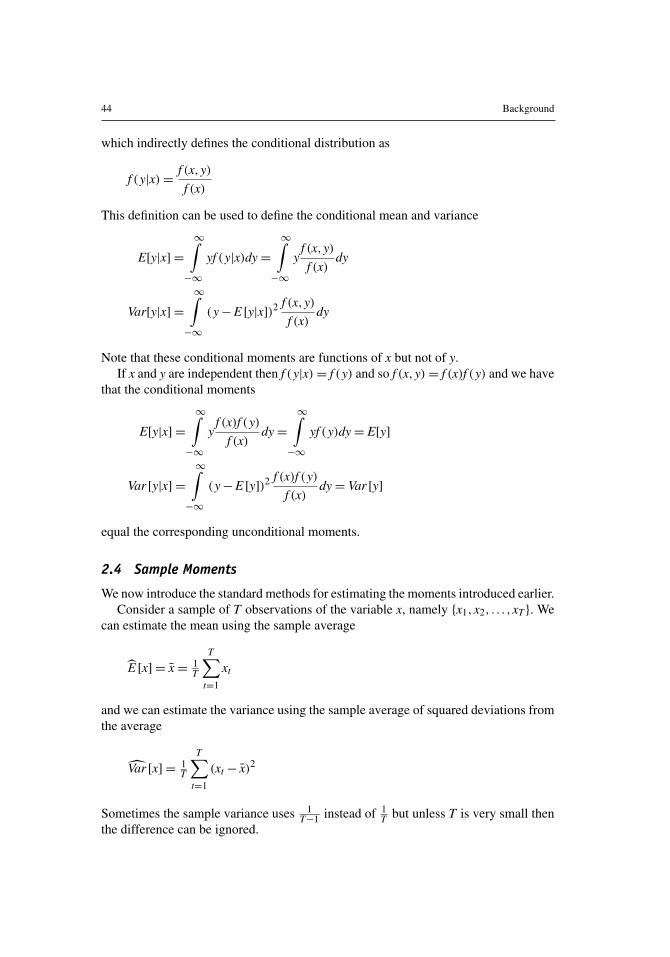
which indirectly defines the conditional distribution as

f (y|x)=f (x,y)

f (x)

This definition can be used to define the conditional mean and variance

E[y|x]=

∞∫−∞

yf (y|x)dy=

∞∫−∞

yf (x,y)

f (x)dy

Var[y|x]=

∞∫−∞

(y−E [y|x])2f (x,y)

f (x)dy

Note that these conditional moments are functions of x but not of y.If x and y are independent then f (y|x)= f (y) and so f (x,y)= f (x)f (y) and we have

that the conditional moments

E[y|x]=

∞∫−∞

yf (x)f (y)

f (x)dy=

∞∫−∞

yf (y)dy= E[y]

Var [y|x]=

∞∫−∞

(y−E [y])2f (x)f (y)

f (x)dy= Var [y]

equal the corresponding unconditional moments.

2.4 Sample Moments

We now introduce the standard methods for estimating the moments introduced earlier.Consider a sample of T observations of the variable x, namely {x1,x2, . . . ,xT}. We

can estimate the mean using the sample average

E [x]= x= 1T

T∑t=1

xt

and we can estimate the variance using the sample average of squared deviations fromthe average

Var [x]= 1T

T∑t=1

(xt− x)2

Sometimes the sample variance uses 1T−1 instead of 1

T but unless T is very small thenthe difference can be ignored.


Similarly skewness and kurtosis can be estimated by

Skew [x]= 1T

T∑t=1

(xt− x)3 /Var [x]3/2

Kurt [x]= 1T

T∑t=1

(xt− x)4 /Var [x]2

The sample covariances between two random variables can be estimated via

Cov [x,y]= 1T

T∑t=1

(xt− x)(yt− y)

and the sample correlation between two random variables, x and y, is calculated as

ρx,y =

∑Tt=1 (xt− x)(yt− y)√∑T

t=1 (xt− x)2∑T

t=1 (yt− y)2

3 The Linear Model

Risk managers often rely on linear models of the type

y= a+ bx+ ε

where E [ε]= 0 and x and ε are assumed to be independent or sometimes just uncor-related. If we know the value of x then we can use the linear model to predict y via theconditional expectation of y given x

E [y|x]= a+ bE [x|x]+E [ε|x]= a+ bx

In the linear model the unconditional expectations of x and y are linked via

E [y]= a+ bE [x]+E [ε]= a+ bE [x]

so that

a= E [y]− bE [x]

We also have that

Cov [y,x]= Cov [a+ bx+ ε,x]= bCov [x,x]= bVar [x]

46 Background

so that

b=Cov [y,x]

Var [x]

In the linear model the variances of x and y are linked via

Var [y]= b2Var [x]+Var [ε]

Consider observation t in the linear model

yt = a+ bxt+ εt

If we have a sample of T observations then we can estimate

b=Cov [x,y]

Var [x]=

∑Tt=1 (xt− x)(yt− y)∑T

t=1 (xt− x)2

and

a= y− bx

In the more general linear model with J different x-variables we have

yt = a+J∑

j=1

bjxj,t+ εt

Minimizing the sum of squared errors,∑T

t=1 ε2t provides the ordinary least square

(OLS) estimate of b:

b= argminT∑

t=1

ε2t = argmin

T∑t=1

yt− a−J∑

j=1

bjxj,t

2

The solution to this optimization problem is a linear function of y and x, which makesOLS estimation very easy to perform; thus it is built in to most common quantita-tive software packages such as Excel, where the OLS estimation function is calledLINEST.

3.1 The Importance of Data Plots

While the linear model is useful in many cases, an apparent linear relationship betweentwo variables can be deceiving. Consider the four (artificial) data sets in Table 3.1,


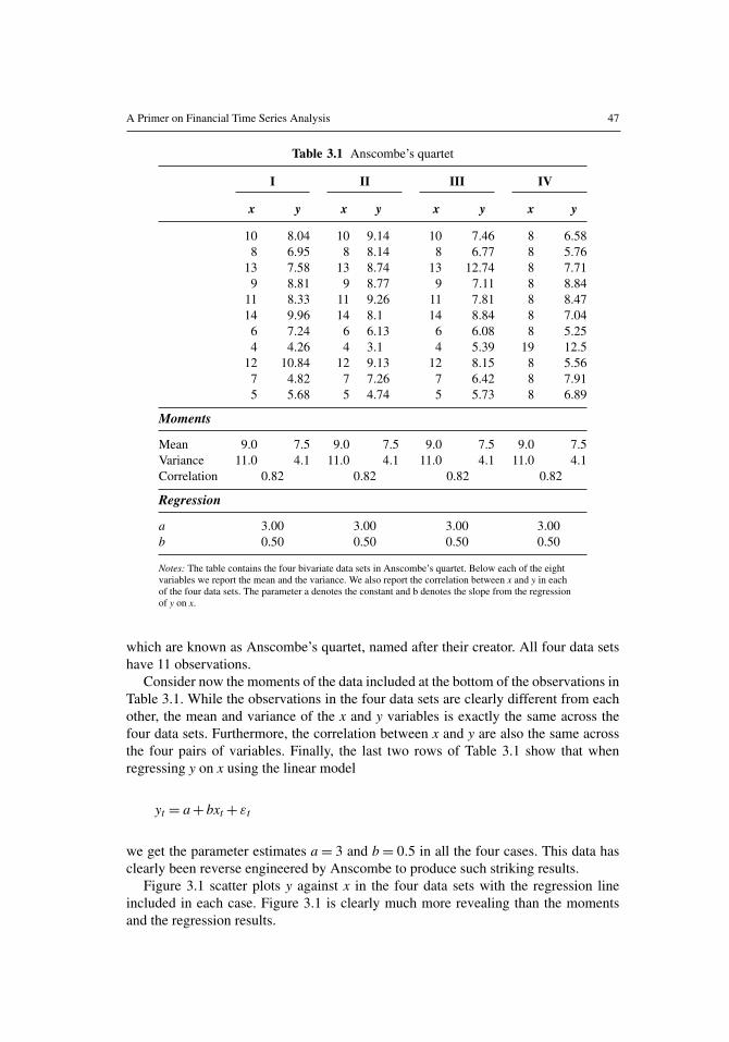
Table 3.1 Anscombe’s quartet

I II III IV

x y x y x y x y

10 8.04 10 9.14 10 7.46 8 6.588 6.95 8 8.14 8 6.77 8 5.76

13 7.58 13 8.74 13 12.74 8 7.719 8.81 9 8.77 9 7.11 8 8.84

11 8.33 11 9.26 11 7.81 8 8.4714 9.96 14 8.1 14 8.84 8 7.04

6 7.24 6 6.13 6 6.08 8 5.254 4.26 4 3.1 4 5.39 19 12.5

12 10.84 12 9.13 12 8.15 8 5.567 4.82 7 7.26 7 6.42 8 7.915 5.68 5 4.74 5 5.73 8 6.89

Moments

Mean 9.0 7.5 9.0 7.5 9.0 7.5 9.0 7.5Variance 11.0 4.1 11.0 4.1 11.0 4.1 11.0 4.1Correlation 0.82 0.82 0.82 0.82

Regression

a 3.00 3.00 3.00 3.00b 0.50 0.50 0.50 0.50

Notes: The table contains the four bivariate data sets in Anscombe’s quartet. Below each of the eightvariables we report the mean and the variance. We also report the correlation between x and y in eachof the four data sets. The parameter a denotes the constant and b denotes the slope from the regressionof y on x.

which are known as Anscombe’s quartet, named after their creator. All four data setshave 11 observations.

Consider now the moments of the data included at the bottom of the observations inTable 3.1. While the observations in the four data sets are clearly different from eachother, the mean and variance of the x and y variables is exactly the same across thefour data sets. Furthermore, the correlation between x and y are also the same acrossthe four pairs of variables. Finally, the last two rows of Table 3.1 show that whenregressing y on x using the linear model

yt = a+ bxt+ εt

we get the parameter estimates a= 3 and b= 0.5 in all the four cases. This data hasclearly been reverse engineered by Anscombe to produce such striking results.

Figure 3.1 scatter plots y against x in the four data sets with the regression lineincluded in each case. Figure 3.1 is clearly much more revealing than the momentsand the regression results.

48 Background

Figure 3.1 Scatter plot of Anscombe’s four data sets with regression lines.

00 5 10 15 20

2468

101214

x

y

00 5 10 15 20

2468

101214

x

y

00 5 10 15 20

2468

101214

x

y

00 5 10 15 20

2468

101214

x

y

I II

III IV

Notes: For each of the four data sets in Anscombe’s quartet we scatter plot the variables andalso report the regression line from fitting y on x.

We conclude that moments and regressions can be useful for summarizing variablesand relationships between them but whenever possible it is crucial to complement theanalysis with figures. When plotting your data you may discover:

l A genuine linear relationship as in the top-left panel of Figure 3.1

l A genuine nonlinear relationship as in the top-right panel

l A biased estimate of the slope driven by an outlier observation as in the bottom-leftpanel

l A trivial relationship, which appears as a linear relationship again due to an outlieras in the bottom-right panel of Figure 3.1

Remember: Always plot your variables before beginning a statistical analysis ofthem.

4 Univariate Time Series Models

Univariate time series analysis studies the behavior of a single random variableobserved over time. Risk managers are interested in how prices and risk factors moveover time; therefore time series models are useful for risk managers. Forecasting thefuture values of a variable using past and current observations on the same variable isa key topic in univariate time series analysis.


4.1 Autocorrelation

Correlation measures the linear dependence between two variables and autocorrelationmeasures the linear dependence between the current value of a time series variable andthe past value of the same variable. Autocorrelation is a crucial tool for detecting lineardynamics in time series analysis.

The autocorrelation for lag τ is defined as

ρτ ≡ Corr[Rt,Rt−τ

]=

Cov [Rt,Rt−τ ]√Var [Rt]Var [Rt−τ ]

=Cov [Rt,Rt−τ ]

Var [Rt]

so that it captures the linear relationship between today’s value and the value τ daysago.

Consider a data set on an asset return, {R1,R2, . . . ,RT}. The sample autocorrelationat lag τ measures the linear dependence between today’s return, Rt, and the return τdays ago, Rt−τ . Using the autocorrelation definition, we can write the sample autocor-relation as

ρτ =

1T−τ

∑Tt=τ+1

(Rt−R

)(Rt−τ −R

)1T

∑Tt=1

(Rt−R

)2 , τ = 1,2, . . . ,m< T

In order to detect dynamics in a time series, it is very useful to first plot the autocor-relation function (ACF), which plots ρτ on the vertical axis against τ on the horizontalaxis.

The statistical significance of a set of autocorrelations can be formally tested usingthe Ljung-Box statistic. It tests the null hypothesis that the autocorrelation for lags 1through m are all jointly zero via

LB(m)= T(T + 2)m∑τ=1

ρ2τ

T − τ∼ χ2

m

where χ2m denotes the chi-squared distribution with m degrees of freedom.

The critical value of χ2m corresponding to the probability p can be found for exam-

ple by using the CHIINV function in Excel. If p= 0.95 and m= 20, then the for-mula CHIINV(0.95,20) in Excel returns the value 10.85. If the test statistic LB(20)computed using the first 20 autocorrelations is larger than 10.85 then we reject thehypothesis that the first 20 autocorrelations are zero at the 5% significance level.

Clearly, the maximum number of lags, m, must be chosen in order to implementthe test. Often the application at hand will give some guidance. For example if we arelooking to detect intramonth dynamics in a daily return, we use m= 21 correspondingto 21 trading days in a month. When no such guidance is available, setting m= ln(T)has been found to work well in simulation studies.

50 Background

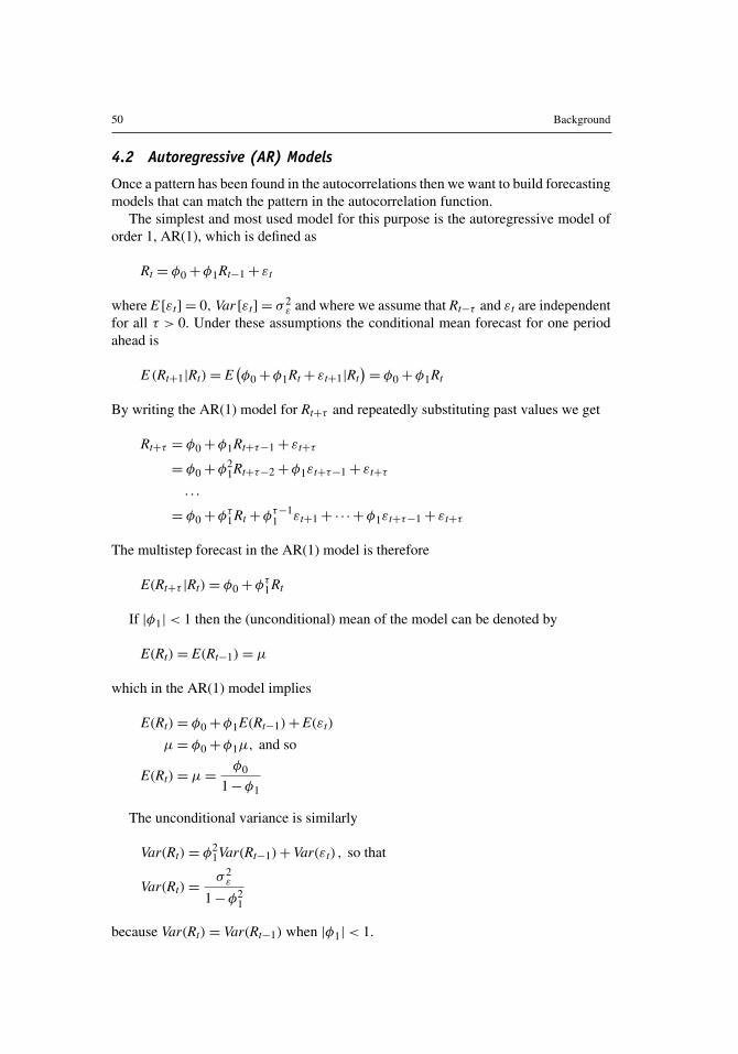
4.2 Autoregressive (AR) Models

Once a pattern has been found in the autocorrelations then we want to build forecastingmodels that can match the pattern in the autocorrelation function.

The simplest and most used model for this purpose is the autoregressive model oforder 1, AR(1), which is defined as

Rt = φ0+φ1Rt−1+ εt

where E [εt]= 0, Var [εt]= σ 2ε and where we assume that Rt−τ and εt are independent

for all τ > 0. Under these assumptions the conditional mean forecast for one periodahead is

E (Rt+1|Rt)= E(φ0+φ1Rt+ εt+1|Rt

)= φ0+φ1Rt

By writing the AR(1) model for Rt+τ and repeatedly substituting past values we get

Rt+τ = φ0+φ1Rt+τ−1+ εt+τ

= φ0+φ21Rt+τ−2+φ1εt+τ−1+ εt+τ

. . .

= φ0+φτ1Rt+φ

τ−11 εt+1+ ·· ·+φ1εt+τ−1+ εt+τ

The multistep forecast in the AR(1) model is therefore

E(Rt+τ |Rt)= φ0+φτ1Rt

If |φ1|< 1 then the (unconditional) mean of the model can be denoted by

E(Rt)= E(Rt−1)= µ

which in the AR(1) model implies

E(Rt)= φ0+φ1E(Rt−1)+E(εt)

µ= φ0+φ1µ, and so

E(Rt)= µ=φ0

1−φ1

The unconditional variance is similarly

Var(Rt)= φ21Var(Rt−1)+Var(εt) , so that

Var(Rt)=σ 2ε

1−φ21

because Var(Rt)= Var(Rt−1) when |φ1|< 1.


Just as time series data can be characterized by the ACF then so can linear timeseries models. To derive the ACF for the AR(1) model assume without loss of gener-ality that µ= 0. Then

Rt = φ1Rt−1+ εt, and

RtRt−τ = φ1Rt−1Rt−τ + εtRt−τ , and so

E (RtRt−τ )= φ1E (Rt−1Rt−τ ), which implies

ρτ = φ1ρτ−1, so that

ρτ = φτ1ρ0 = φ

τ1

This provides the ACF of the AR(1) model. Notice the similarity between the ACFand the multistep forecast earlier.

The lag order τ appears in the exponent of φ1 and we therefore say that the ACFof an AR(1) model decays exponentially to zero as τ increases. The case when φ1 isclose to 1 but not quite 1 is important in financial economics. We refer to this as ahighly persistent series.

Figure 3.2 shows examples of the ACF in AR(1) models with four different (posi-tive) values of φ1. When φ1<1 then the ACF decays to zero exponentially. Clearlythe decay is much slower when φ1=0.99 than when it is 0.5 or 0.1. When φ1=1 thenthe ACF is flat at 1. This is the case of a random walk, which we will study furtherlater.

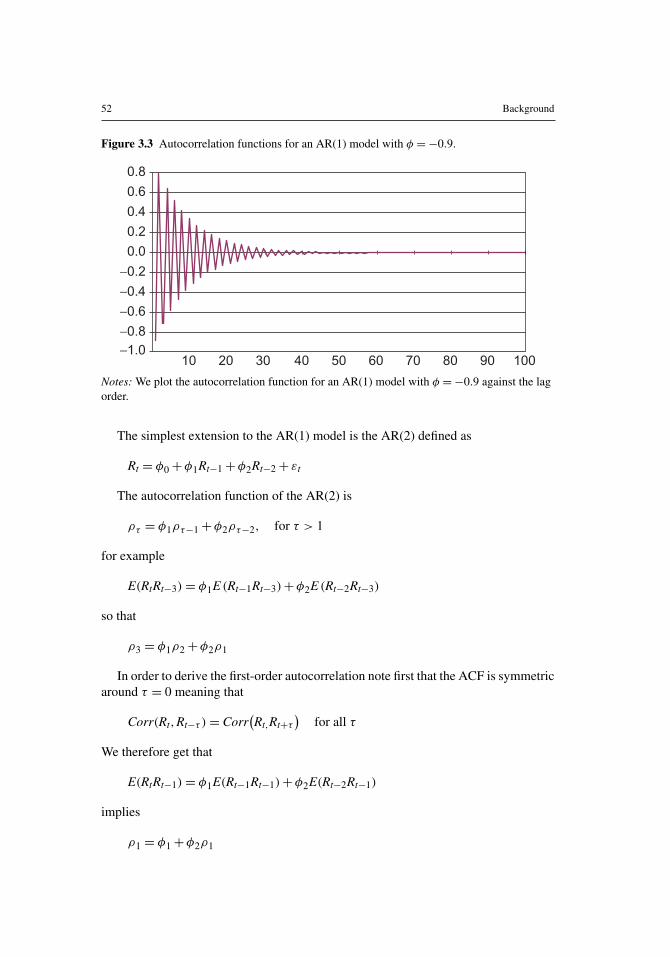
Figure 3.3 shows the ACF of an AR(1) when φ1 =−0.9. Notice the drasticallydifferent ACF pattern compared with Figure 3.2. When φ1<0 then the ACF oscillatesaround zero but it still decays to zero as the lag order increases. The ACFs in Figure 3.2are much more common in financial risk management than are the ACFs in Figure 3.3.

Figure 3.2 Autocorrelation functions for AR(1) models with positive φ1.

0

0.2

0.4

0.6

0.8

1

1.2

10 20 30 40 50 60 70 80 90 100

φ =1

φ = 0.99

φ = 0.5

φ = 0.1

Notes: We plot the autocorrelation function for four AR(1) processes with different values ofthe autoregressive parameter φ1. When φ1<1 then the ACF decays to 0 at an exponential rate.

52 Background

Figure 3.3 Autocorrelation functions for an AR(1) model with φ =−0.9.

−1.0

−0.8

−0.6

−0.4

−0.2

0.0

0.2

0.4

0.6

0.8

10 20 30 40 50 60 70 80 90 100

Notes: We plot the autocorrelation function for an AR(1) model with φ =−0.9 against the lagorder.

The simplest extension to the AR(1) model is the AR(2) defined as

Rt = φ0+φ1Rt−1+φ2Rt−2+ εt

The autocorrelation function of the AR(2) is

ρτ = φ1ρτ−1+φ2ρτ−2, for τ > 1

for example

E(RtRt−3)= φ1E (Rt−1Rt−3)+φ2E (Rt−2Rt−3)

so that

ρ3 = φ1ρ2+φ2ρ1

In order to derive the first-order autocorrelation note first that the ACF is symmetricaround τ = 0 meaning that

Corr(Rt,Rt−τ )= Corr(Rt,Rt+τ

)for all τ

We therefore get that

E(RtRt−1)= φ1E(Rt−1Rt−1)+φ2E(Rt−2Rt−1)

implies

ρ1 = φ1+φ2ρ1


so that

ρ1 =φ1

1−φ2

The general AR(p) model is defined by

Rt = φ0+φ1Rt−1+ ·· ·+φpRt−p+ εt

The one-step ahead forecast in the AR(p) model is simply

Et(Rt+1)≡ E(Rt+1|Rt,Rt−1, . . .

)= φ0+φ1Rt+ ·· ·+φpRt+1−p

The τ day ahead forecast can be built using

Et (Rt+τ )= φ0+

p∑i=1

φiEt(Rt+τ−i)

which is sometimes called the chain-rule of forecasting. Note that when τ < i then

Et(Rt+τ−i)= Rt+τ−i

because Rt+τ−i is known at the time the forecast is made when τ < i.The partial autocorrelation function (PACF) gives the marginal contribution of an

additional lagged term in AR models of increasing order. First estimate a series of ARmodels of increasing order:

Rt = φ0,1+φ1,1Rt−1+ ε1t

Rt = φ0,2+φ1,2Rt−1+φ2,2Rt−2+ ε2t

Rt = φ0,3+φ1,3Rt−1+φ2,3Rt−2+φ3,3Rt−3+ ε3t

......

The PACF is now defined as the collection of the largest order coefficients{φ1,1,φ2,2,φ3,3, . . .

}which can be plotted against the lag order just as we did for the ACF.

The optimal lag order p in the AR(p) can be chosen as the largest p such that φp,pis significant in the PACF. For example, an AR(3) will have a significant φ3,3 but itwill have a φ4,4 close to zero.

Note that in AR models the ACF decays exponentially whereas the PACF decaysabruptly. This is why the PACF is useful for AR model order selection.

The AR(p) models can be easily estimated using simple OLS regression on obser-vations p+ 1 through T . A useful diagnostic test of the model is to plot the ACF ofresiduals from the model and perform a Ljung-Box test on the residuals using m− pdegrees of freedom.

54 Background

4.3 Moving Average (MA) Models

In AR models the ACF dies off exponentially, however, certain dynamic features suchas bid-ask bounces or measurement errors die off abruptly and require a different typeof model. Consider the MA(1) model in which

Rt = θ0+ εt+ θ1εt−1

where εt and εt−1 are independent of each other and where E [εt]= 0. Note that

E [Rt]= θ0

and

Var(Rt)= (1+ θ21)σ

2ε

In order to derive the ACF of the MA(1) assume without loss of generality thatθ0 = 0. We then have

Rt = εt+ θ1εt−1 which implies

Rt−τRt = Rt−τ εt+ θ1Rt−τ εt−1, so that

E(Rt−1Rt)= θ1σ2ε , and

E(Rt−τRt)= 0, for τ > 1

Using the variance expression from before, we get the ACF

ρ1 =θ1

1+ θ21

, and

ρτ = 0, for τ > 1

Note that the autocorrelations for the MA(1) are zero for τ > 1.Unlike AR models, the MA(1) model must be estimated by numerical optimization

of the likelihood function. We proceed as follows. First, set the unobserved ε0 = 0,which is its expected value. Second, set parameter starting values (initial guesses) forθ0, θ1, and σ 2

ε . We can use the average of Rt for θ0, use 0 for θ1, and use the samplevariance of Rt for σ 2

ε . Now we can compute the time series of residuals via

εt = Rt− θ0− θ1εt−1, with ε0 = 0

We are now ready to estimate the parameters by maximizing the likelihood functionthat we must first define. Let us first assume that εt is normally distributed, then

f (εt)=1(

2πσ 2ε

)1/2 exp

(−ε2

t

2σ 2ε

)


To construct the likelihood function note that as the εts are independent over time wehave

f (ε1,ε2, . . . ,εT)= f (ε1) f (ε2) . . . f (εT)

and we therefore can write the joint distribution of the sample as

f (ε1,ε2, . . . ,εT)=

T∏t=1

1(2πσ 2

ε

)1/2 exp

(−ε2

t

2σ 2ε

)

The maximum likelihood estimation method chooses parameters to maximize theprobability of the estimated model (in this case MA(1)) having generated the observeddata set (in this case the set of Rts).

In the MA(1) model we must perform an iterative search (using for example Solverin Excel) over the parameters θ0,θ1,σ

2ε :

L(

R1, . . . ,RT |θ0,θ1,σ2ε

)=

T∏t=1

1(2πσ 2

ε

)1/2 exp

(−ε2

t

2σ 2ε

)where εt = Rt− θ0− θ1εt−1, with ε0 = 0

Once the parameters have been estimated we can use the model for forecasting. Inthe MA(1) model the conditional mean forecast is

E(Rt+1|Rt,Rt−1, . . .)= θ0+ θ1εt

E(Rt+τ |Rt,Rt−1, . . .)= θ0, for τ > 1

The general MA(q) model is defined by

Rt = θ0+ θ1εt−1+ θ2εt−2+ ·· ·+ θqεt−q+ εt

It has an ACF that is nonzero for the first q lags and then zero for lags larger than q.Note that MA models are easily identified using the ACF. If the ACF of a data

series dies off to zero abruptly after the first four (nonzero) lags then an MA(4) islikely to provide a good fit of the data.

4.4 Combining AR and MA into ARMA Models

Parameter parsimony is key in forecasting, and combining AR and MA models intoARMA models often enables us to model dynamics with fewer parameters.

Consider the ARMA(1,1) model, which includes one lag of Rt and one lag of εt:

Rt = φ0+φ1Rt−1+ θ1εt−1+ εt

56 Background

As in the AR(1), the mean of the ARMA(1,1) time series is given from

E [Rt]= φ0+φ1E [Rt−1]= φ0+φ1E [Rt]

which implies that

E(Rt)=φ0

1−φ1

when∣∣φ1

∣∣< 1. In this case Rt will tend to fluctuate around the mean, φ0/(1−φ1

),

over time. We say that Rt is mean-reverting in this case.Using the fact that E [Rtεt]= σ 2

ε we can get the variance from

Var [Rt]= φ21Var [Rt]+ θ

21σ

2ε + σ

2ε + 2φ1θ1σ

2ε

which implies that

Var(Rt)=(1+ 2φ1θ1+ θ

21)σ

2ε

1−φ21

The first-order autocorrelation is given from

E [RtRt−1]= φ1E [Rt−1Rt−1]+ θ1E [εt−1Rt−1]+E [εtRt−1]

in which we assume again that φ0 = 0. This implies that

ρ1Var(Rt)= φ1Var(Rt)+ θ1σ2ε

so that

ρ1 = φ1+θ1σ

2ε

Var(Rt)

For higher order autocorrelations the MA term has no effect and we get the samestructure as in the AR(1) model

ρτ = φ1ρτ−1, for τ > 1

The general ARMA(p,q) model is

Rt = φ0+

p∑i=1

φiRt−i+

q∑i=1

θ iεt−i+ εt

Because of the MA term, ARMA models just as MA models must be estimatedusing maximum likelihood estimation (MLE). Diagnostics on the residuals can bedone via Ljung-Box tests with degrees of freedom equal to m− q− p.


4.5 Random Walks, Units Roots, and ARIMA Models

The random walk model is a key benchmark in financial forecasting. It is often usedto model speculative prices in logs. Let St be the closing price of an asset and letst = ln(St) so that log returns are immediately defined by Rt ≡ ln(St)− ln(St−1)=

st− st−1.The random walk (or martingale) model for log prices is now defined by

st = st−1+ εt

By iteratively substituting in lagged log prices we can write

st = st−2+ εt−1+ εt

. . .

st = st−τ + εt−τ+1+ εt−τ+2+ ·· ·+ εt

Because past εt−τ residual (or shocks) matter equally and fully for st regardless of τwe say that past shocks have permanent effects in the random walk model.

In the random walk model, the conditional mean and variance forecasts for the logprice are

Et(st+τ )= st

Vart(st+τ )= τσ2ε

Note that the forecast for s at any horizon is just today’s value, st. We therefore some-times say that the random walk model implies that the series is not predictable. Notealso that the conditional variance of the future value is a linear function of the forecasthorizon, τ .

Equity returns typically have a small positive mean corresponding to a small driftin the log price. This motivates the random walk with drift model

st = µ+ st−1+ εt

Substituting in lagged prices back to time 0, we have

st = tµ+ s0+ εt+ εt−1+ ·· ·+ ε1

Notice that in this model the constant drift µ in returns corresponds to a coefficient ontime, t, in the log price model. We call this a deterministic time trend and we refer tothe sum of the εs as a stochastic trend.

A time series, st, follows an ARIMA(p,1,q) model if the first differences, st− st−1,follow a mean-reverting ARMA(p,q) model. In this case we say that st has a unit root.The random walk model has a unit root as well because in that model

st− st−1 = εt

which is a trivial ARMA(0,0) model.

58 Background

4.6 Pitfall 1: Spurious Mean-Reversion

Consider the AR(1) model again:

st = φ1st−1+ εt⇔

st− st−1 = (φ1− 1)st−1+ εt

Note that when φ1 = 1 then the AR(1) model has a unit root and becomes the randomwalk model. The OLS estimator contains an important small sample bias in dynamicmodels. For example, in an AR(1) model when the true φ1 coefficient is close or equalto 1, the finite sample OLS estimate will be biased downward. This is known as theHurwitz bias or the Dickey-Fuller bias. This bias is important to keep in mind.

If φ1 is estimated in a small sample of asset prices to be 0.85 then it implies thatthe underlying asset price is predictable and market timing thus feasible. However,the true value may in fact be 1, which means that the price is a random walk and sounpredictable.

The aim of technical trading analysis is to find dynamic patterns in asset prices.Econometricians are very skeptical about this type of analysis exactly because itattempts to find dynamic patterns in prices and not returns. Asset prices are likelyto have a φ1 very close to 1, which in turn is likely to be estimated to be somewhatlower than 1, which in turn suggests predictability. Asset returns have a φ1 close tozero and the estimate of an AR(1) on returns does not suffer from bias. Looking fordynamic patterns in asset returns is much less likely to produce false evidence of pre-dictability than is looking for dynamic patterns in asset returns. Risk managers oughtto err on the side of prudence and thus consider dynamic models of asset returns andnot asset prices.

4.7 Testing for Unit Roots

Asset prices often have a φ1 very close to 1. But we are very interested in knowingwhether φ1 = 0.99 or 1 because the two values have very different implications forlonger term forecasting as indicated by Figure 3.2. φ1 = 0.99 implies that the assetprice is predictable so that market timing is possible whereas φ1 = 1 implies it is not.Consider again the AR(1) model with and without a constant term:

st = φ0+φ1st−1+ εt

st = φ1st−1+ εt

Unit root tests (also known as Dickey-Fuller tests) have been developed to assess thenull hypothesis

H0 : φ1 = 1

against the alternative hypothesis that

HA : φ1 < 1


This looks like a standard t-test in a regression but it is crucial that when the nullhypothesis H0 is true, so that φ1 = 1, the unit root test does not have the usual normaldistribution even when T is large. If you estimate φ1 using OLS and test that φ1 = 1using the usual t-test with critical values from the normal distribution then you arelikely to reject the null hypothesis much more often than you should. This means thatyou are likely to spuriously find evidence of mean-reversion, that is, predictability.

5 Multivariate Time Series Models

Multivariate time series analysis is relevant for risk management because we oftenconsider risk models with multiple related risk factors or models with many assets.This section will briefly introduce the following important topics: time series regres-sions, spurious relationships, cointegration, cross correlations, vector autoregressions,and spurious causality.

5.1 Time Series Regression

The relationship between two (or more) time series can be assessed applying the usualregression analysis. But in time series analysis the regression errors must be scruti-nized carefully.

Consider a simple bivariate regression of two highly persistent series, for example,the spot and futures price of an asset

s1t = a+ bs2t+ et

The first step in diagnosing such a time series regression model is to plot the ACFof the regression errors, et.

If ACF dies off only very slowly (the Hurwitz bias will make the ACF look likeit dies off faster to zero than it really does) then it is good practice to first-differenceeach series and run the regression

(s1t− s1t−1)= a+ b(s2t− s2t−1)+ et

Now the ACF can be used on the residuals of the new regression and the ACFcan be checked for dynamics. The AR, MA, or ARMA models can be used to modelany dynamics in et. After modeling and estimating the parameters in the residual timeseries, et, the entire regression model including a and b can be reestimated using MLE.

5.2 Pitfall 2: Spurious Regression

Checking the ACF of the error term in time series regressions is particularly importantdue to the so-called spurious regression phenomenon: Two completely unrelated timesseries—each with a unit root—are likely to appear related in a regression that has asignificant b coefficient.

60 Background

Specifically, let s1t and s2t be two independent random walks

s1t = s1t−1+ ε1t

s2t = s2t−1+ ε2t

where ε1t and ε2t are independent of each other and independent over time. Clearlythe true value of b is zero in the time series regression

s1t = a+ bs2t+ et

However, in practice, standard t-tests using the estimated b coefficient will tend toconclude that b is nonzero when in truth it is zero. This problem is known as spuriousregression.

Fortunately, as noted earlier, the ACF comes to the rescue for detecting spuriousregression. If the relationship between s1t and s2t is spurious then the error term, et,

will have a highly persistent ACF and the regression in first differences

(s1t− s1t−1)= a+ b(s2t− s2t−1)+ et

will not show a significant estimate of b. Note that Pitfall 1, earlier, was related to mod-eling univariate asset prices time series in levels rather than in first differences. Pitfall2 is in the same vein: Time series regression on highly persistent asset prices is likelyto lead to false evidence of a relationship, that is, a spurious relationship. Regressionon returns is much more likely to lead to sensible conclusions about dependence acrossassets.

5.3 Cointegration

Relationships between variables with unit roots are of course not always spurious.A variable with a unit root, for example a random walk, is also called integrated, andif two variables that are both integrated have a linear combination with no unit rootthen we say they are cointegrated.

Examples of cointegrated variables could be long-run consumption and productionin an economy, or the spot and the futures price of an asset that are related via ano-arbitrage condition. Similarly, consider the pairs trading strategy that consists offinding two stocks whose prices tend to move together. If prices diverge then we buythe temporarily cheap stock and short sell the temporarily expensive stock and waitfor the typical relationship between the prices to return. Such a strategy hinges on thestock prices being cointegrated.

Consider a simple bivariate model where

s1t = φ0+ s1,t−1+ ε1t

s2t = bs1t+ ε2t

Note that s1t has a unit root and that the level of s1t and s2t are related via b. Assumethat ε1t and ε2t are independent of each other and independent over time.


The cointegration model can be used to preserve the relationship between the vari-ables in the long-term forecasts

E(s1,t+τ |s1t,s2t

)= φ0τ + s1t

E(s2,t+τ |s1t,s2t

)= bφ0τ + bs1t

The concept of cointegration was developed by Rob Engle and Clive Granger. Theytogether received the Nobel Prize in Economics in 2003 for this and many other con-tributions to financial time series analysis.

5.4 Cross-Correlations

Consider again two financial time series, R1,t and R2,t. They can be dependent inthree possible ways: R1,t can lead R2,t (e.g., Corr

(R1,t,R2,t+1

)6= 0), R1,t can lag

R2,t (e.g., Corr(R1,t+1,R2,t

)6= 0), and they can be contemporaneously related (e.g.,

Corr(R1,t,R2,t

)6= 0). We need a tool to detect all these possible dynamic relationships.

The sample cross-correlation matrices are the multivariate analogues of the ACFfunction and provide the tool we need. For a bivariate time series, the cross-covariancematrix for lag τ is

0τ =

[Cov

(R1,t,R1,t−τ

)Cov

(R1,t,R2,t−τ

)Cov

(R2,t,R1,t−τ

)Cov

(R2,t,R2,t−τ

)] , τ ≥ 0

Note that the two diagonal terms are the autocovariance function of R1,t, and R2,t,respectively.

In the general case of a k-dimensional time series, we have

0τ = E{(Rt−E [Rt])(Rt−τ −E [Rt])

′}, τ ≥ 0

where Rt is now a k by 1 vector of variables.Detecting lead and lag effects is important, for example when relating an illiquid

stock to a liquid market factor. The illiquidity of the stock implies price observationsthat are often stale, which in turn will have a spuriously low correlation with the liquidmarket factor. The stale equity price will be correlated with the lagged market factorand this lagged relationship can be used to compute a liquidity-corrected measure ofthe dependence between the stock and the market.

5.5 Vector Autoregressions (VAR)

The vector autoregression model (VAR), which is not to be confused with Value-at-Risk (VaR), is arguably the simplest and most often used multivariate time seriesmodel for forecasting. Consider a first-order VAR, call it VAR(1)

Rt = φ0+8Rt−1+ εt, Var(εt)=6

where Rt is again a k by 1 vector of variables.

62 Background

The bivariate case is simply

R1,t = φ0,1+811R1,t−1+812R2,t−1+ ε1,t

R2,t = φ0,1+821R1,t−1+822R2,t−1+ ε2,t

6 =

[σ 2

1 σ 12

σ 21 σ22

]Note that in the VAR, R1,t and R2,t are contemporaneously related via their covari-

ance σ 12 = σ 21. But just as in the AR model, the VAR only depends on lagged vari-ables so that it is immediately useful in forecasting.

If the variables included on the right-hand-side of each equation in the VAR arethe same (as they are above) then the VAR is called unrestricted and OLS can be usedequation-by-equation to estimate the parameters.

5.6 Pitfall 3: Spurious Causality

We may sometimes be interested to see if the lagged value of R2,t, namely R2,t−1, iscausal for the current value of R1,t, in which case it can be used in forecasting. To thisend a simple regression of the form

R1,t = a+ bR2,t−1+ et

could be used. Note that it is the lagged value R2,t−1 that appears on the right-handside. Unfortunately, such a regression may easily lead to false conclusions if R1,t ispersistent and so depends on its own past value, which is not included on the right-hand side of the regression.

In order to truly assess if R2,t−1 causes R1,t (or vice versa), we should ask thequestion: Is past R2,t useful for forecasting current R1,t once the past R1,t has beenaccounted for? This question can be answered by running a VAR model:

R1,t = φ0,1+811R1,t−1+812R2,t−1+ ε1,t

R2,t = φ0,2+821R1,t−1+822R2,t−1+ ε2,t

Now we can define Granger causality (as opposed to spurious causality) as follows:

l R2,t is said to Granger cause R1,t if 812 6= 0

l R1,t is said to Granger cause R2,t if 821 6= 0

In some cases several lags of R1,t may be needed on the right-hand side of theequation for R1,t and similarly we may need more lags of R2,t in the equation for R2,t.

6 Summary

The financial asset prices and portfolio values typically studied by risk managers canbe viewed as examples of very persistent time series. An important goal of this chapter


is therefore to ensure that the risk manager avoids some common pitfalls that arisebecause of the persistence in prices. The three most important issues are

l Spurious detection of mean-reversion; that is, erroneously finding that a variable ismean-reverting when it is truly a random walk

l Spurious regression; that is, erroneously finding that a variable x is significant whenregressing y on x

l Spurious detection of causality; that is, erroneously finding that the current valueof x causes (helps determine) future values of y when in reality it cannot

Several more advanced topics have been left out of the chapter including longmemory models and models of seasonality. Long memory models give more flexi-bility in modeling the autocorrelation function (ACF) than do the traditional ARIMAand ARMA models studied in this chapter. In particular long-memory models allowfor the ACF to go to zero more slowly than the AR(1) model, which decays to zero atan exponential decay as we saw earlier. Seasonal models are useful, for example, forthe analysis of agricultural commodity prices where seasonal patterns in supply causeseasonal patterns in prices, in expected returns, and in volatility. These topics can bestudied using the resources suggested next.

Further Resources

For a basic introduction to financial data analysis, see Koop (2006) and for an intro-duction to probability theory see Paollela (2006). Wooldridge (2002) and Stock andWatson (2010) provide a broad introduction to econometrics. Anscombe (1973) con-tains the data in Table 3.1 and Figure 3.1.

The univariate and multivariate time series material in this chapter is based onChapters 2 and 8 in Tsay (2002), which should be consulted for various extensionsincluding seasonality and long memory. See also Taylor (2005) for an excellent treat-ment of financial time series analysis focusing on volatility modeling.

Diebold (2004) gives a thorough introduction to forecasting in economics. Grangerand Newbold (1986) is the classic text for the more advanced reader. Christoffersenand Diebold (1998) analyze long-horizon forecasting in cointegrated systems.

The classic references on the key time series topics in this chapter are Hurwitz(1950) on the bias in the AR(1) coefficient, Granger and Newbold (1974) on spuriousregression in economics, Engle and Granger (1987) on cointegration, Granger (1969)on Granger causality, and Dickey and Fuller (1979) on unit root testing. Hamilton(1994) provides an authoritative treatment of economic time series analysis.

Tables with critical values for unit root tests can be found in MacKinnon (1996,2010). See also Chapter 14 in Davidson and MacKinnon (2004).

References

Anscombe, F.J., 1973. Graphs in statistical analysis. Am. Stat. 27, 17–21.Christoffersen, P., Diebold, F., 1998. Cointegration and long horizon forecasting. J. Bus. Econ.

Stat. 16, 450–458.

64 Background

Davidson, R., MacKinnon, J.G., 2004. Econometric Theory and Methods. Oxford UniversityPress, New York, NY.

Dickey, D.A., Fuller, W.A., 1979. Distribution of the estimators for autoregressive time serieswith a unit root. J. Am. Stat. Assoc. 74, 427–431.

Diebold, F.X., 2004. Elements of Forecasting, third ed. Thomson South-Western, Cincinnati,Ohio.

Engle, R.F., Granger, C.W.J., 1987. Co-integration and error correction: Representation, esti-mation and testing. Econometrica 55, 251–276.

Granger, C.W.J., 1969. Investigating causal relations by econometric models and cross-spectralmethods. Econometrica 37, 424–438.

Granger,C.W.J.,Newbold,P.,1974.Spurious regressions ineconometrics. J.Econom.2,111–120.Granger, C.W.J., Newbold, P., 1986. Forecasting Economic Time Series, second ed. Academic

Press, Orlando, FL.Hamilton, J.D., 1994. Time Series Analysis. Princeton University Press, Princeton, NJ.Hurwitz, L., 1950. Least squares bias in time series. In: Koopmans, T.C. (Ed.), Statistical Infer-

ence in Econometric Models. Wiley, New York, NY.Koop, G., 2006. Analysis of Financial Data. Wiley, Chichester, West Sussex, England.MacKinnon, J.G., 1996. Numerical distribution functions for unit root and cointegration tests.

J. Appl. Econom. 11, 601–618.MacKinnon, J.G., 2010. Critical Values for Cointegration Tests, Queen’s Economics Depart-

ment. Working Paper no 1227. http://ideas.repec.org/p/qed/wpaper/1227.html.Paollela, M., 2006. Fundamental Probability. Wiley, Chichester, West Sussex, England.Stock, J., Watson, M., 2010. Introduction to Econometrics, second ed. Pearson Addison Wesley.Taylor, S.J., 2005. Asset Price Dynamics, Volatility and Prediction. Princeton University Press,

Princeton, NJ.Tsay, R., 2002. Analysis of Financial Time Series. Wiley Interscience, Hoboken, NJ.Wooldridge, J., 2002. Introductory Econometrics: A Modern Approach. Second Edition. South-

Western College Publishing, Mason, Ohio.

Empirical Exercises

Open the Chapter3Data.xlsx file from the web site.

1. Using the data in the worksheet named Question 3.1 reproduce the moments and regressioncoefficients at the bottom of Table 3.1.

2. Reproduce Figure 3.1.3. Reproduce Figure 3.2.4. Using the data sets in the worksheet named Question 3.4, estimate an AR(1) model on each

of the 100 columns of data. (Excel hint: Use the LINEST function.) Plot the histogram of the100 φ1 estimates you have obtained. The true value of φ1 is one in all the columns. Whatdoes the histogram tell you?

5. Using the data set in the worksheet named Question 3.4, estimate an MA(1) model usingmaximum likelihood. Use the starting values suggested in the text. Use Solver in Excel tomaximize the likelihood function.

Answers to these exercises can be found on the companion site.

For more information see the companion site athttp://www.elsevierdirect.com/companions/9780123744487

3 A Primer on Financial Time Series Analysis · PDF file3 A Primer on Financial Time Series...

Documents

Transcript of 3 A Primer on Financial Time Series Analysis · PDF file3 A Primer on Financial Time Series...