an author's http://oatao.univ-toulouse.fr/21983

http://doi.org/10.1002/qre.2446

Atamuradov, Vepa and Medjaher, Kamal and Camci, Fatih and Zerhouni, Noureddine and Dersin, Pierre andLamoureux, Benjamin Feature selection and fault severity classification–based machine health assessmentmethodology for point machine sliding chair degradation. (2019) Quality and Reliability Engineering International.1-19. ISSN 0748-8017

Feature selection and fault‐severity classification–based

machine health assessment methodology for point machine

sliding‐chair degradation

Vepa Atamuradov1 | Kamal Medjaher2 | Fatih Camci3 | Noureddine Zerhouni4 |

Pierre Dersin5 | Benjamin Lamoureux5

1Assystem Energy & Infrastructure,

Imagine Laboratory, Courbevoie, France

2Production Engineering Laboratory

(LGP), Toulouse University, INPT‐ENIT,

Tarbes, France

3Amazon Inc., Austin, Texas, USA

4FEMTO‐ST, UMR CNRS‐UFC/ENSMM,

France

5ALSTOM Transport, France

Correspondence

Vepa Atamuradov, Assystem Energy &

Infrastructure, Imagine Laboratory, Tour

Egée 11 Allée de l'Arche, Courbevoie,

France.

Email: vatamuradov@assystem.com

Abstract

In this paper, we propose an offline and online machine health assessment

(MHA) methodology composed of feature extraction and selection,

segmentation‐based fault severity evaluation, and classification steps. In the

offline phase, the best representative feature of degradation is selected by a

new filter‐based feature selection approach. The selected feature is further seg-

mented by utilizing the bottom‐up time series segmentation to discriminate

machine health states, ie, degradation levels. Then, the health state fault severity

is extracted by a proposed segment evaluation approach based on within seg-

ment rate‐of‐change (RoC) and coefficient of variation (CV) statistics. To train

supervised classifiers, a priori knowledge about the availability of the labeled

data set is needed. To overcome this limitation, the health state fault‐severity

information is used to label (eg, healthy, minor, medium, and severe) unlabeled

raw condition monitoring (CM) data. In the online phase, the fault‐severity clas-

sification is carried out by kernel‐based support vector machine (SVM) classifier.

Next to SVM, the k‐nearest neighbor (KNN) is also used in comparative analysis

on the fault severity classification problem. Supervised classifiers are trained in

the offline phase and tested in the online phase. Unlike to traditional supervised

approaches, this proposedmethod does not require any a priori knowledge about

the availability of the labeled data set. The proposedmethodology is validated on

infield point machine sliding‐chair degradation data to illustrate its effectiveness

and applicability. The results show that the time series segmentation‐based fail-

ure severity detection and SVM‐based classification are promising.

KEYWORDS

fault severity, fault‐severity classification, filter‐based feature selection, inferential statistics, machine

health assessment, point machine sliding‐chair degradation, time series segmentation

1 | INTRODUCTION

Safety, reliability, and availability have been concerned as one of the important and challenging issues for different

industries to meet the market requirements while increasing the production quantity and quality. Hence, it's essential

to develop a more robust monitoring systems that can control and assess the health state of the components before they

fall into a critical stage.

Machine health assessment (MHA) can be described as an inspection process of the degradation by monitoring the

machine health state transitions in order to determine the state changes due to anomalies and extract the fault severity

information from the condition monitoring (CM) data.1 Hence, the MHA information can be used in the development

of failure diagnostics and prognostics algorithms for complex systems CM (eg, railway infrastructure,2,3 wind turbines,4

rotating machinery5, nuclear power plants,6 and electric vehicles7).

Railway point machines are one of the complex structures in railway infrastructure, which are used to control the

train turnouts at a distance. Thus, it is important to monitor the point machine components' health states in order to

increase operational reliability, availability, and passengers safety.8 The accuracy of data–driven‐based MHA methods

depends on extraction and selection of good features from the raw CM data. The better feature captures the machine

degradation, the better is the CM information can be achieved.

In literature, feature extraction techniques are categorized as time based, frequency‐based, and time‐frequency based,9

whereas feature selection methods are classified as a filter, wrapper, and embedded methods.10 The filter‐based methods

use general properties of the features to filter the least interesting ones using some ranking threshold (eg, correlation,

monotonicity, prognosability, trendability,11 and seperability12). The wrappermethods use evolutionary or searching algo-

rithms (eg, particle swarm optimization [PSO]13) to find the optimumnumber of features thatmaximize the objective func-

tion of the given algorithm. The embedded feature selection methods combine filter and wrapper methods14 in order to

build good features for CM. In a previous study,15 the authors proposed a feature extraction methodology for diagnostics

of point machines using empirical mode decomposition (EMD) and singular value decomposition (SVD) for fault detec-

tion. In literature, there are plenty of works conducted in feature extraction and selection problem applied for gearbox,16,17

bearings,12,18 batteries,19 and point machine20 monitoring using different CM data types. It is important to note that,

despite the variety of feature selection techniques, it is hard to have a generic feature selection technique, which is superior

to others.21 Thus, the feature extraction and selection process play an important role in fault detection, diagnostics, and

prognostics of degrading systems, and there are still many issues to be tackled to build good machine health indicators.

Fault detection methods study the change of machine health state magnitudes by measuring the statistics of fault

propagation to characterize them as normal or faulty. In literature, the fault detection and diagnostics has been exten-

sively studied for point machine monitoring by using machine learning and signal processing tools. For example, the

authors in a previous research22 studied the fault detection and classification of point machine using discrete wavelet

transform (DWT) and support vector machine (SVM). The DWT was used in feature reduction, whereas the SVM

was trained to classify the failure modes. Similarly, a fault diagnostics approach was also presented by the authors in

other studies20,23 based on the principal component analysis (PCA) and SVM classifier using the extracted statistical fea-

tures. Similar works for fault detection of point machines have been studied in literature as well.24,25 Next to machine

learning tools, statistical techniques were also used in point machine CM.

A simple statistical fault detection methodology for anomaly detection by using dynamic time warping (DTW) met-

ric was presented in a previous study.26 The methodology was validated using the infield point machine Direct Current

(DC) data. In the same domain, a generic fault detection methodology was proposed in another study27 based on seg-

ment evaluation, data fusion, and inferential statistics for point machine CM. An expert fault identification and detec-

tion system was proposed for point machine CM in an existing research,8 using simulated point machine data. First of

all, generated failure data were denoised using the moving average (MA) smoother, and the DTW was utilized in health

state detection afterward. Similarly, a fault detection approach using Kolmogorov‐Smirnov (K‐S) test statistics for point

machine monitoring was proposed in another study.28 The authors simulated sliding chair and obstacle on stock rail

failure modes, and the method was validated using the point machine DC current signatures for failure detection. A

statistical process control‐based fault detection and prognostics approach has been investigated in another wotk29 for

train gearbox using extracted vibration features.

The fault detection only deals with the identification of normal and faulty processes from the CM data but cannot

provide any fault severity information about the degradation after detection. The fault severity (magnitude) information

can be used in MHA to make decisions whether to trigger diagnostics/prognostics tasks or not.

The fault severity evaluation can be defined as an analysis of degradation levels to retrieve severity information

about machine health states. The fault severity information can be used in fault diagnostics and prognostics to support

decision making.

A point machine failure prognostics methodology based on state durations was proposed in an existing study.30,31

The authors utilized k‐means clustering in the point machine health states identification and calculated the state

transition probabilities for prognostics by using hidden Markov models (HMMs). In the same domain, a data–driven‐

based point MHA methodology was proposed in a previous research32 for failure prognostics. In this work, the point

machine degradation levels were extracted and the remaining‐useful‐life (RUL) was calculated using the state transition

time values. The authors in a previous study33 proposed a systematic health assessment methodology based on self‐

organizing maps (SOMs) and PCA techniques for point machine fault diagnostics. In this work, different statistical fea-

tures were extracted from the segmented power signals. The extracted features were further used in point machine

degradation‐level assessment and incipient fault detection. An air leakage detection and failure prediction approach

for the train braking system was proposed in another study34 based on regression and clustering. The regression classi-

fier was used in failure severity prediction, and the density‐based clustering was utilized to detect the leakage anomalies.

However, clustering‐based degradation level detection, ie, health state or fault severity detection, approaches may not

guarantee that the change in health state transitions are due to the machine degradation. Because, the clusters, ie,

health states, found by these tools may refer to variations of the operational conditions, rather than the variation due

to degradation, which is one of the disadvantages of using unsupervised learning for fault detection and severity eval-

uation. In addition, the clusters extracted by using any clustering algorithms can be different,35 and therefore may

not be a consistent approach for machine health state detection.

To fill the aforementioned gaps in literature, this paper proposes a new MHA methodology for point machine deg-

radation, particularly through feature selection, fault detection, and severity classification. Furthermore, although there

are plenty of works that studied fault severity evaluation and classification problem for bearings1,36,37 and gearboxes,38 to

the best of our knowledge, the problem of fault severity evaluation is not explicitly studied for railway point MHA. The

proposed MHA methodology for point machine CM is composed of offline and online phases, as shown in Figure 1.

The main contributions of this current work can be summarized as follows:

• Proposition of a new two‐step filter‐based prognostics feature selection approach. Compared with the wrapper and

ensemble approaches, our filter‐based approach is computationally efficient and effective.

• Development and application of a time series segmentation and inferential–statistics‐based fault detection and fault

severity evaluation approach. Unlike HMM and clustering‐based techniques, the segmentation‐based approach is

computationally less consuming and more robust against the nonmonotonicity problem in fault detection.

• Unlike traditional supervised fault classification approaches, the proposed method does not require any a priori

knowledge about the availability of the labeled data. The data are labeled automatically using the fault severity infor-

mation derived from segment evaluation algorithm.

The paper is organized as follows: Section 2 explains the proposed methodology. The data collection procedure for

point machine sliding‐chair monitoring is explained in Section 3. The results of proposed methodology are discussed in

Section 4. Section 5 concludes the paper.

FIGURE 1 The proposed methodology workflow [Colour figure can be viewed at wileyonlinelibrary.com]

2 | METHODOLOGY

In this section, the offline and online phases of the proposed health assessment methodology will be explained.

In the offline phase, a new filter‐based feature selection approach is developed to select the best representative

feature. The feature selection is carried out in two steps. In step 1, an affinity matrix is built from the feature pool to

calculate interclass similarities and relative importance weights. In step 2, degradation parameters of the features such

as monotonicity, correlation, and robustness are calculated. A linearly weighted fitness function is then constructed by

combining the interclass (ie, relative importance weights) and intraclass (ie, degradation parameters) feature analysis

steps for feature selection. The best feature should have the highest fitness value. Afterwards, the selected feature is

segmented by utilizing the bottom‐up (BUP) time series segmentation39 algorithm to extract the machine health states,

ie, degradation levels. Then, a within feature segment analysis is performed using the coefficient of variations (CV)40

and the rate‐of‐change (RoC), ie, slope,41 statistics to derive the segment fault severity for classification. Finally, the fault

severity information is used to label (eg, healthy, medium, and severe) the unlabeled raw data for fault severity

classification.

In the online phase, the fault severity classification for sliding‐chair monitoring is carried out by a kernel‐based SVM

classifier. Next to SVM, the k‐nearest neighbor (KNN) is also presented in comparative analysis on the fault severity

classification problem. Then, supervised classifiers are trained in the offline phase and tested in the online phase.

Finally, the proposed methodology is implemented on infield point machine sliding‐chair degradation data, which were

collected from the real system, to illustrate its effectiveness and applicability.

2.1 | Feature extraction and selection

In this paper, time–domain‐based feature extraction techniques such as skewness, root mean square (rms), kurtosis,

mean, standard deviation (stdev), variance (var), crest factor (crfactor), and peak‐to‐peak (p2p) are used in sliding‐chair

health assessment. Extracted statistical features with different degradation behaviors (eg, increasing or decreasing) in

different scales should be first normalized before selection. The features are normalized and put into standard scale

and form by using Equations 1 and 2. Equation 1 is used to normalize the features with decreasing trend, and Equation 2

is used to normalize the features with increasing trend.

F i ¼Di − min Dið Þð Þ

max Dið Þ − min Dið Þð Þ; where Di;t ¼

f i;t

max f ið Þ; (1)

F i ¼Di − min Dið Þð Þ

max Dið Þ − min Dið Þð Þ; where Di;t ¼

min f ið Þ

f i;t: (2)

f i, t is the ith feature data point at time index t (t = 1…T), T is the feature length, and F i is the ith normalized feature.

After the normalization process, all features have the same standard scale of degradation.

The feature selection is carried out in two steps. In step 1, the affinity matrix (Equation 4) is built using the Euclid-

ean distance (Equation 3).

dist p; qð Þ ¼

ffiffiffiffiffiffiffiffiffiffiffiffiffiffiffiffiffiffiffiffiffiffiffiffiffiffiffi

∑Ni¼1 pi−qið Þ2

q

; (3)

where N is the length of the given features p and q.

Affinity ¼

dist f 1; f 1ð Þ ⋯ dist f 1; fMð Þ

⋮ ⋱ ⋮

dist fM ; f 1ð Þ ⋯ dist fM ; fMð Þ

2

6

4

3

7

5

M×M

; (4)

where dist( f 1, fM) is the Euclidean distance between the features f 1 and fM from the feature pool with a length of M.

The relative importance weight wi of ith (∀i = 1…M) feature is calculated by using the normalized similarity mean

(μi) value and exponential membership function (Equation 6). A feature with the minimum interclass distance is

assigned with the highest weight (w) value in the feature selection.

μi ¼ ∑Mi¼1dist

f i;1

M

) *

; (5)

wi ¼ exp −1 × μið Þ: (6)

In step 2, degradation parameters of features such as monotonicity (Moni), correlation (Corri), and robustness (Robi)

are calculated using Equations 7, 8, and 9 . The features' monotonicity parameter is used to extract either increasing or

decreasing trend information. The features' correlation measures the linearity statistics between features' degradation

health states and time. The robustness parameter stands for the features' resistance to the measurement noise. The cor-

relation parameter utilized in this paper is based on the Pearson's correlation coefficient.10

Moni f ið Þ ¼

#d

df i> 0

N − 1−

#d

df i< 0

N − 1

+

+

+

+

+

+

+

+

+

+

+

+

+

+

+

+

0

B

B

@

1

C

C

A

; (7)

where Moni is the monotonicity value for the ith feature ( f i) with length of N. The absolute value of the difference

between number of positive #d

df i> 0

) *

and negative #d

df i< 0

) *

derivatives gives the monotonicity value. A feature

with the higher monotonicity indicates the better degradation with an increasing/decreasing trend.

Corri f i;T ið Þ ¼cov f i;T ið Þ

σfiσTi

) *

; (8)

where cov is the covariance of ith feature ( f i) with the time vector T and σ is the standard deviation. To calculate the

features' robustness, first of all, the given feature should be decomposed into trend and residual components. The

residual component (resfi) of the feature f i is extracted by subtracting the smoothed feature smoothed_ f i (trend) from

the original (noisy) feature f i, as given in Equation 9.

resf i ¼ f i − smoothed f i; (9)

Robi f ið Þ ¼

∑Nn exp −

resf if i

+

+

+

+

+

+

+

+

) *

N

0

B

B

@

1

C

C

A

; (10)

where N is the length of ith feature ( f i). Then, the goodness of the feature is evaluated using the linearly weighted fitness

function, which is given in Equation 11.

fitnessi ¼ ∑M

i¼1

wi × Moni;Corri;Rubi½ %: (11)

Consequently, a feature with the highest fitness (max[fitnessi = 1 : M]) value is then selected as the best feature and

used in fault detection and fault severity evaluation step. We also present a comparative analysis between our feature

selection approach and the work proposed in another study,42 to show the effectiveness and efficiency in the feature

selection problem, which will be covered in the results and discussions section.

2.2 | Fault detection and fault severity evaluation by time series segmentation

Time series segmentation has been studied and applied in many applications, such as security43 and machine fault

detection27,44 as well. The time series segmentation is the decomposition process of series into homogeneous groups

with similar characteristics. In this paper, the BUP time series segmentation technique39 is used in fault detection

and fault severity evaluation. The BUP, which is the piecewise linear approximation technique, relies on divide and

merge strategy. The two adjacent segments are merged by calculating the cost function, and the same procedure is

repeated iteratively until the stopping criteria are met. Interested readers can refer to this39 paper for more information

about the BUP time series segmentation. A pseudocode for the BUP algorithm is given in Table 1.

Since the BUP decomposes the given feature into homogenous subsequences, each segment can be treated as a dif-

ferent machine health state with different degradation levels. Thus, the feature segments can be used in MHA for fault

detection and fault severity evaluation. Generally, all segmentation techniques are supervised, and they need a

predefined threshold or segment number a priori before the segmentation. Therefore, a segment evaluation is needed

to optimize the segment numbers to get the best homogeneous segments.

An inferential statistics, which is CV,40 and the RoC are used in this paper for segment optimization, fault detection,

and fault severity identification. The RoC can be defined as a ratio between the change in data points over a specific

period of time. In this study, the RoC is used to measure the within segment degradation rates. The within segment

RoC is calculated by using Equation 12 and fed to Equation 13. The CV is the measure of dispersion that measures

the variability of points around the mean. The advantage of CV is it is dimensionless and can be used in comparative

analysis of different measures. The CV is the ratio of the standard deviation (σ) to the mean (μ), as given in Equation 13.

We assume that if there is a significant change (ie, either minimum or maximum) in CV distribution of calculated

within segment RoC values, this is due to between segment heterogeneity, and this can be interpreted as an optimum

number for time series segmentation. The between segment heterogeneity can be defined as the dissimilarity of

segments with different statistical characteristics. The main goal in time series segmentation is to decompose the given

feature into homogenous groups while increasing the between segment heterogeneity.

RoCi DFSi;LFSið Þ ¼ ∑diff DFSið Þ

diff LFSið Þ

) *

× 100; (12)

CV s RoCsð Þ ¼ σRoCs=μRoCs

2 3

; (13)

TABLE 1 Bottom‐up time series segmentation pseudocode

Algorithm 1: Seg_BUP (data, max_err)

for i= 1:2:length (data) %Initial segment

Seg_BUP =

concat (Seg_BUP,create_seg(data [i: i+1]));

end

for i = 1: length (Seg_BUP)-1

merge_cost(i) = calc_err(merge (Seg_BUP(i),

Seg_BUP(i+1)));

end

%while not segmented

while min (merge_cost)

% find costless segments to merge

ind = min (merge_cost);

Seg_BUP(ind)= merge (Seg_BUP(ind),

Seg_BUP(ind+1));

% update records

del (Seg_BUP(ind+1));

merge_cost(ind)=calc_err(merge (Seg_BUP(ind,

Seg_BUP(ind+1)));

merge_cost(ind-1)=

calc_err(merge (Seg_BUP(ind-1,

Seg_BUP(ind)));

end

where (DFSi) is the measurement variables within the ith feature segment (FSi), diff(DFSi) is the variable difference, LFSi is

the time indices, and CVs is the dispersion of sth RoC.

The segmentation algorithm is run several times using different segment numbers starting from 2, assuming that the

degraded machine has at least two health states such as healthy and faulty. The calculated RoC values from each

segmentation process is then fed to Equation 13 to select the best number of segments. The significant rise/drop in

CV distribution after the segmentation process is then selected as the optimum segmentation number as follows:

• If RoC values have a decreasing trend, then the optimum number of segmentation is selected by taking the mini-

mum CV value.

• If RoC values have an increasing trend, then the optimum number of segmentation is selected by taking the maxi-

mum CV value.

The trend of the RoC is identified by differencing the RoC values, which is obtained from the first segmentation pro-

cess (ie, using segment number of 2) before checking for the significant change in CV. The whole feature segment eval-

uation algorithm for fault severity evaluation and identification is given in Table 2.

Consequently, the CV and RoC statistics are combined to be used in machine health state severity analysis and time

series segment optimization. The optimized feature segments are assumed as real health states of the machine. The raw

data are then further labeled using the extracted fault severity information from this step and are used for machine fault

severity classification. Next to sliding‐chair degradation data, the proposed segment evaluation algorithm will be also

evaluated on simulated features with different degradation behaviors to demonstrate its effectiveness in time series seg-

ment optimization.

TABLE 2 Segment evaluation algorithm pseudocode

Algorithm 2: Segment_evaluation (data)

% segN: segmentation numbers

% data: prognostics feature

% seg.left and seg.right: left/right segment points

% diff: 1st order derivative

% s: counter

% Std: standard deviation

% optimum_seg: optimized segmentation

segN= [2,3,4,5,6,7,8,9,10];

s=1;

For n= segN

seg= Seg_BUP (data, n)

For i= 1 to length (seg)

y= data (seg(i).left:seg(i).right);

x= (seg(i).left:seg(i).right);

RoCi(y, x) = sum (diff(y)/diff(x))*100;

End

SL{1, c} = RoC;

CVs(RoC) = std(RoC)/mean(RoC));

s=s+1;

End

optimum_Segment (SL, CV):

If (SL {1,1}(1,2) - SL {1,1}(1,1))

% decreasing trend

ind = min (CV)

optimum_seg= SL{1, ind}

Else

% increasing trend

ind = max (CV)

optimum_seg= SL{1, ind}

2.3 | Fault severity classification

In fault severity classification, supervised ML tools can be adopted to classify the machine fault severity, ie, the degra-

dation level. There are several supervised ML tools used in classification problems such as decision trees, Artificial Neu-

ral Networks (ANN), and SVM. The SVM classifier is chosen in this study due to its good accuracy and capability of

performing linear and nonlinear data classification.45

The SVM, which was introduced by Vapnik,46 is a very popular machine‐learning classification tool. The initial prin-

ciple of SVM is to separate given data into distinct two classes by using a linear hyperplane. The linear separation of two

classes can be achieved by finding an optimum decision hyperplane that maximizes the margin between two imaginary

parallel planes (support vectors). In SVM, the kernel function describes the similarity measure of given data points. The

kernel selection has been accepted as one of the major problems in SVM classification. There are several kernel func-

tions used in SVM‐based classifications. In this paper, three kernel types—linear, polynomial, and Gaussian—are used

to compare fault severity classification results. Interested readers are referred to previous studies47,48 for more detailed

information about SVM classification with kernel functions.

The proposed point machine sliding‐chair MHA model takes raw measurements as an input and predicts the

machine fault severity levels as an output, which is illustrated in Figure 2.

3 | CASE STUDY

In this section, the railway point machine system, data collection, and the accelerated degradation modeling will be

explained. The point machine sliding‐chair monitoring data are used in the further evaluation of the proposed health

assessment methodology.

3.1 | Railway point machine

The point machines (also known as turnout machines), which are one of the critical and complex components of rail-

way infrastructure, are used to control train turnouts by providing track changing at a distance. To ensure availability,

reliability and safe operation, point machines require regular inspections, and maintenance next to improved CM

systems.

3.1.1 | Data collection and accelerated aging procedure

The electromechanical point machine (Figure 3), which is investigated and monitored in this paper, consists of one DC

motor, a gearbox, two drive rods (to move rails back‐and‐forth), and electric peripherals. Different sensors (see Figure 3)

were installed on the point machine components (eg, drive rods, cables, and rails) to monitor and collect degradation

data. Figure 4 shows the collected force, DC current, voltage, and proximity sensor data from the point machine. CM

data collected by the force and current sensors are the most commonly used sensors in the literature49 for point machine

diagnostics and prognostics. In this study, the force degradation data are used in fault detection and severity classifica-

tion. The CM data were collected from both “back‐and‐forth” movements of the point machine.

FIGURE 2 Model input‐output relation

Since point machines are complex systems with different subcomponents, they have many failure modes. Some

failure modes develop over a long period of time that makes fault detection challenging.50 One of the solutions to

overcome this problem and spend less time in tracking seldom seen and/or slowly progressive failures can be to gener-

ate failure modes by the accelerated aging procedure. This latter procedure can be defined as manually contaminating

FIGURE 3 Railway point machine and installed sensors [Colour figure can be viewed at wileyonlinelibrary.com]

FIGURE 4 Collected condition monitoring sensory time series [Colour figure can be viewed at wileyonlinelibrary.com]

(ie, soiling or scratching out the grease) the sliding‐chair plate to obtain slowly progressive failures in a short amount of

time. In this research, only the dry sliding‐chair failure mode is studied, and the infield CM data are collected via

installed sensors during the accelerated aging procedure on the real system.

Sliding‐chair plates are the metal assets of the turnout system that assist point machine drive rods in moving the rail

blades easily. Typical sliding‐chair plates installed on wooden traverses of turnout system are illustrated in Figure 5.

Sliding‐chair degradation data were collected from the real Turkish State Railways point machine in Tekirdag, Turkey.

This turnout system has 12 sliding‐chair plates in total. Initially, all sliding‐chair plates were dry or contaminated. At

first, all 12 plates were individually lubricated, and the point machine was run 10 times in each movement to get the

first healthy (fault free) CM sensory data. Afterward, the contamination (sprinkling dust or sand) process took place

by soiling three farthest (10th, 11th, and 12th) sliding chairs from the point machine to get an initial faulty state. The sec-

ond faulty state was created by soiling the 9th sliding‐chair plate after the first contamination process. The accelerated

failure modeling process was repeated until a final and complete sliding‐chair faulty state is created. After each step of

the contamination process, the point machine was run 10 times from normal‐to‐reverse (forth) and reverse‐to‐normal

(back) positions to collect the sensory data. The contamination on sliding‐chair plates results in variation of perfor-

mance measurement signals (eg, force, current, and voltage) due to the increasing friction force against the turnout driv-

ing rod force applied to move the blades from normal‐to‐reverse (forth) or reverse‐to‐normal (back) positions. The total

number of degradation data collected in each state is 20 (10 in back and 10 in forth movements). Figure 5 shows the

accelerated sliding‐chair degradation modeling procedure on the turnout with 12 wooden traverses (Tr.). Please note

that no trains went through the turnout system during the data acquisition operation. The turnout system was tempo-

rarily reserved as a test bench for the sliding‐chair failure modeling and data collection purposes only.

4 | RESULTS AND DISCUSSIONS

In this research, only the force degradation data from the normal‐to‐reverse (forth) movement are used to illustrate the

proposed methodology.

FIGURE 5 Accelerated sliding‐chair plate failure modeling [Colour figure can be viewed at wileyonlinelibrary.com]

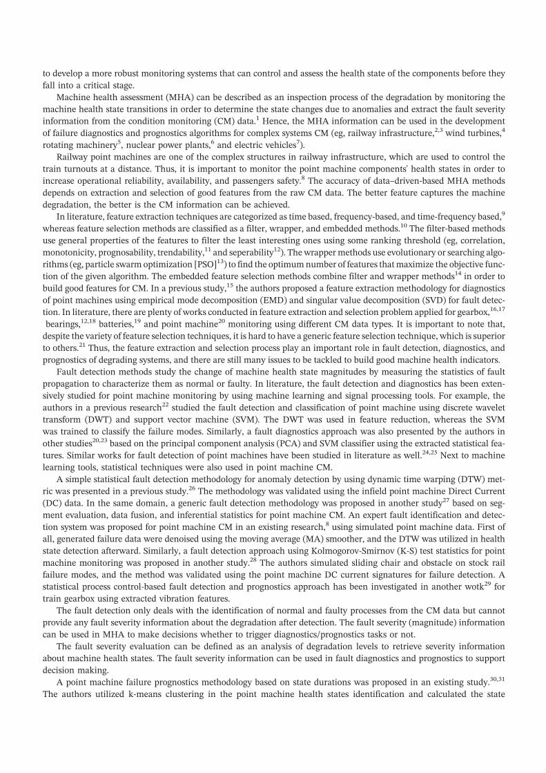
Time–domain‐based statistical features (Figure 6) were extracted from the raw force data and normalized (Figure 7)

by using Equations 1 and 2. The normalized features were then used in feature selection by using the proposed filter‐

based feature selection approach.

The feature selection was carried out in two steps. In step 1, the affinity matrix (Equation 4) was built from the nor-

malized feature pool to calculate interclass similarities and relative features' importance weights (Equation 6). In step 2,

degradation parameters such as monotonicity, correlation, and robustness were calculated using Equations 7, 8, and 10.

The normalized features were smoothed before calculating the monotonicity and correlation parameters. The linearly

weighted fitness function (Equation 11), which combines the interclass (ie, between similarity) and the intraclass (ie,

within degradation parameter) feature analysis steps, was built to select the best feature. The proposed feature selection

approach was also compared with the feature selection method proposed in another study.42 The linear fitness function

in the previous study42 was built by multiplying the monotonicity, correlation, and robustness parameters with the

weights of 0.5, 0.2, and 0.3, which was chosen by the user. Step 1 results are given in Table 3, and step 2 results are given

in Table 5. Table 4 shows assigned features' weights used in the feature selection. As seen from Table 3, the mean, stdev,

and rms, which have the highest relative similarity values to the feature population, can be ranked as the best three

FIGURE 6 Extracted time‐domain features from force time series [Colour figure can be viewed at wileyonlinelibrary.com]

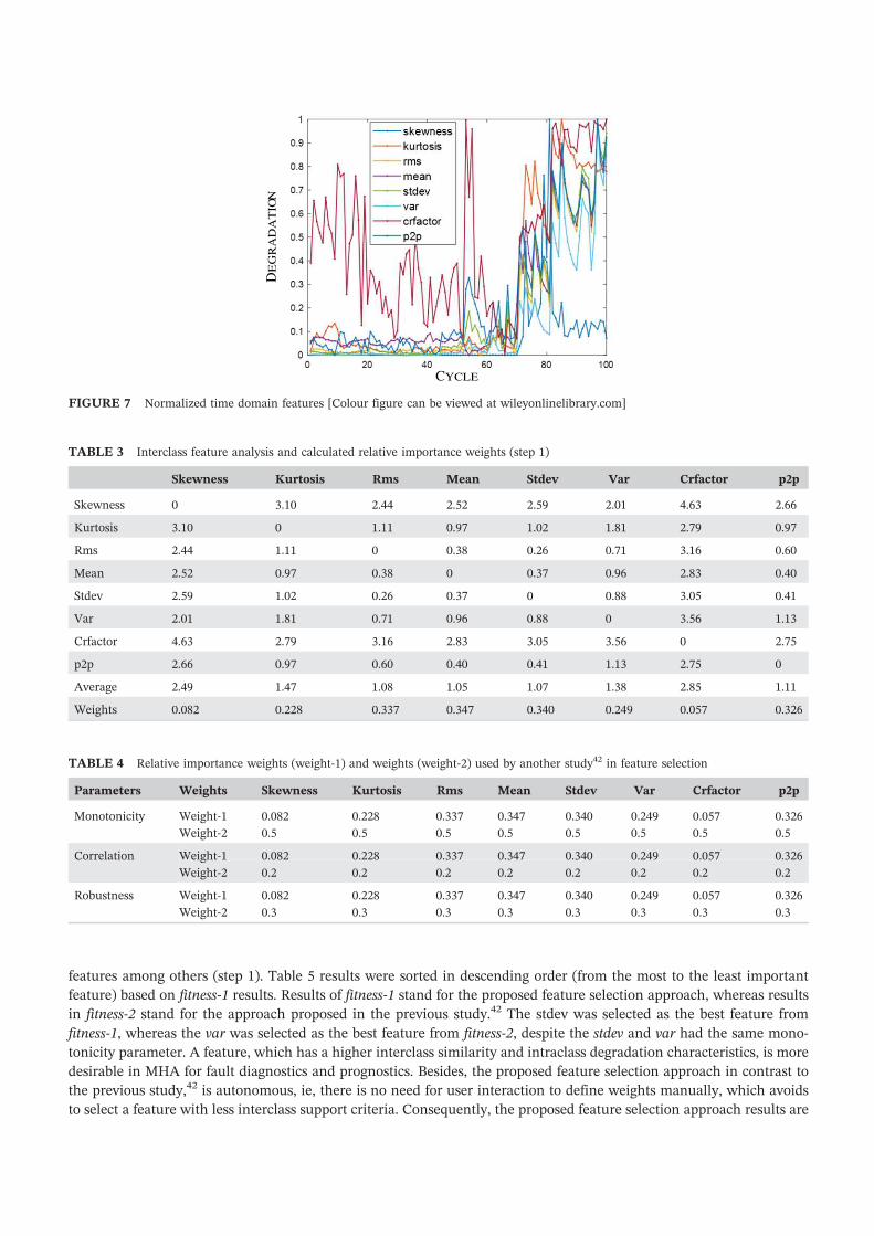
features among others (step 1). Table 5 results were sorted in descending order (from the most to the least important

feature) based on fitness‐1 results. Results of fitness‐1 stand for the proposed feature selection approach, whereas results

in fitness‐2 stand for the approach proposed in the previous study.42 The stdev was selected as the best feature from

fitness‐1, whereas the var was selected as the best feature from fitness‐2, despite the stdev and var had the same mono-

tonicity parameter. A feature, which has a higher interclass similarity and intraclass degradation characteristics, is more

desirable in MHA for fault diagnostics and prognostics. Besides, the proposed feature selection approach in contrast to

the previous study,42 is autonomous, ie, there is no need for user interaction to define weights manually, which avoids

to select a feature with less interclass support criteria. Consequently, the proposed feature selection approach results are

FIGURE 7 Normalized time domain features [Colour figure can be viewed at wileyonlinelibrary.com]

TABLE 3 Interclass feature analysis and calculated relative importance weights (step 1)

Skewness Kurtosis Rms Mean Stdev Var Crfactor p2p

Skewness 0 3.10 2.44 2.52 2.59 2.01 4.63 2.66

Kurtosis 3.10 0 1.11 0.97 1.02 1.81 2.79 0.97

Rms 2.44 1.11 0 0.38 0.26 0.71 3.16 0.60

Mean 2.52 0.97 0.38 0 0.37 0.96 2.83 0.40

Stdev 2.59 1.02 0.26 0.37 0 0.88 3.05 0.41

Var 2.01 1.81 0.71 0.96 0.88 0 3.56 1.13

Crfactor 4.63 2.79 3.16 2.83 3.05 3.56 0 2.75

p2p 2.66 0.97 0.60 0.40 0.41 1.13 2.75 0

Average 2.49 1.47 1.08 1.05 1.07 1.38 2.85 1.11

Weights 0.082 0.228 0.337 0.347 0.340 0.249 0.057 0.326

TABLE 4 Relative importance weights (weight‐1) and weights (weight‐2) used by another study42 in feature selection

Parameters Weights Skewness Kurtosis Rms Mean Stdev Var Crfactor p2p

Monotonicity Weight‐1 0.082 0.228 0.337 0.347 0.340 0.249 0.057 0.326

Weight‐2 0.5 0.5 0.5 0.5 0.5 0.5 0.5 0.5

Correlation Weight‐1 0.082 0.228 0.337 0.347 0.340 0.249 0.057 0.326

Weight‐2 0.2 0.2 0.2 0.2 0.2 0.2 0.2 0.2

Robustness Weight‐1 0.082 0.228 0.337 0.347 0.340 0.249 0.057 0.326

Weight‐2 0.3 0.3 0.3 0.3 0.3 0.3 0.3 0.3

very promising in MHA for fault diagnostics and prognostics. The feature stdev was then fed to the time series segmen-

tation for fault detection and severity identification.

Before segmenting the selected sliding‐chair degradation feature, the proposed segment evaluation and optimization

algorithm was validated on simulated features to test its effectiveness. Two different features with different degradation

behaviors were simulated, as shown in Figure 8 (F1 and F2). The feature F1 has an increasing trend approximately

before the 100‐time index and remains constant for a while before the slightly increasing trend at last stages of its

end‐of‐life (EoF). The feature F2 represents an exponentially progressive degradation with increasing trend. The simu-

lated features were fed to the segment evaluation algorithm to extract health state transitions by within segment eval-

uation. The features were decomposed into different segments, starting from two to 10, and the within segment RoC

values were calculated using Equation 12, as shown in Figure 8 (F1‐RoC and F2‐RoC). The F1‐RoC indicates that the

degradation rate of the F1 decreases as it reaches the EOL, whereas the degradation rate (F2‐RoC) of the F2 increases.

F1 and F2 feature segments had been optimized by using the segment evaluation algorithm given in Table 2, and the

results are depicted in F1‐CV and F2‐CV figures. As a result of segment optimization, F1 was segmented into four

(red circle on F1‐CV) and F2 into three segments (red circle on F2‐CV).

The segmented‐F1 and segmented‐F2 plots in Figure 8 show the decomposed time series results after the optimiza-

tion. The proposed segment evaluation algorithm could effectively optimize the feature segments with different degra-

dation behaviors and can thus be used to detect machine health states.

The feature stdev, which was selected as the best feature, went through the same time series segment optimization

algorithm to identify the degradation levels of the sliding‐chair plates. Figure 9 shows the segment evaluation algorithm

results for the sliding‐chair degradation. The stdev was decomposed into four segments (segmented stdev plot in

Figure 9) indicating the sliding‐chair health state transitions with varying degradation levels. Results of this step were

further used in labeling raw force data for fault severity classification. Table 6 shows the feature segment borders

FIGURE 8 Segment evaluation results for simulated features [Colour figure can be viewed at wileyonlinelibrary.com]

TABLE 5 Intraclass feature analysis and calculated fitness function results (step 2)

Monotonicity Correlation Robustness Fitness‐1 Fitness‐2

Stdev 0.48 0.85 0.42 0.60 0.54

Rms 0.50 0.82 0.42 0.59 0.54

p2p 0.46 0.87 0.40 0.57 0.52

Mean 0.34 0.82 0.40 0.54 0.45

Var 0.48 0.79 0.51 0.44 0.55

Kurtosis 0.22 0.82 0.41 0.33 0.39

Skewness 0.02 0.69 0.66 0.11 0.34

Crfactor 0.26 0.53 0.40 0.06 0.35

(cycles), within segment RoC and assigned data labels. First 42 force time series were labeled as “healthy,” series

between 43 and 60 as “minor,” series between 61 and 72 as “medium,” and series between 73 and 100 as “sever” health

states for sliding‐chair degradation. Figure 10 shows one sample from healthy, minor, medium, and sever force time

series after segment optimization and labeling process, which indicate the sliding‐chair degradation.

FIGURE 9 Segment evaluation algorithm results for the stdev prognostics feature [Colour figure can be viewed at wileyonlinelibrary.com]

TABLE 6 Feature segments and corresponding data labels

Feature segments (Sn, n = 1 … 4)

S1 S2 S3 S4

Cycle (1‐42) (43–60) (61–72) (73–100)

RoC (%) 0.3 5 12 50

Data labels “Healthy” “Minor” “Medium” “Sever”

FIGURE 10 Labeled force time series samples with different degradation levels [Colour figure can be viewed at wileyonlinelibrary.com]

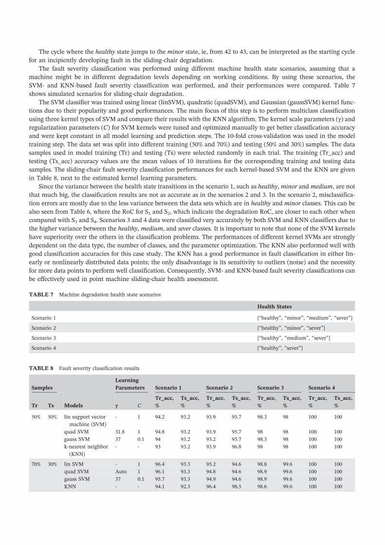
The cycle where the healthy state jumps to the minor state, ie, from 42 to 43, can be interpreted as the starting cycle

for an incipiently developing fault in the sliding‐chair degradation.

The fault severity classification was performed using different machine health state scenarios, assuming that a

machine might be in different degradation levels depending on working conditions. By using these scenarios, the

SVM‐ and KNN‐based fault severity classification was performed, and their performances were compared. Table 7

shows simulated scenarios for sliding‐chair degradation.

The SVM classifier was trained using linear (linSVM), quadratic (quadSVM), and Gaussian (gaussSVM) kernel func-

tions due to their popularity and good performances. The main focus of this step is to perform multiclass classification

using three kernel types of SVM and compare their results with the KNN algorithm. The kernel scale parameters (γ) and

regularization parameters (C) for SVM kernels were tuned and optimized manually to get better classification accuracy

and were kept constant in all model learning and prediction steps. The 10‐fold cross‐validation was used in the model

training step. The data set was split into different training (50% and 70%) and testing (50% and 30%) samples. The data

samples used in model training (Tr) and testing (Ts) were selected randomly in each trial. The training (Tr_acc) and

testing (Ts_acc) accuracy values are the mean values of 10 iterations for the corresponding training and testing data

samples. The sliding‐chair fault severity classification performances for each kernel‐based SVM and the KNN are given

in Table 8, next to the estimated kernel learning parameters.

Since the variance between the health state transitions in the scenario 1, such as healthy, minor and medium, are not

that much big, the classification results are not as accurate as in the scenarios 2 and 3. In the scenario 2, misclassifica-

tion errors are mostly due to the less variance between the data sets which are in healthy and minor classes. This can be

also seen from Table 6, where the RoC for S1 and S2, which indicate the degradation RoC, are closer to each other when

compared with S3 and S4. Scenarios 3 and 4 data were classified very accurately by both SVM and KNN classifiers due to

the higher variance between the healthy, medium, and sever classes. It is important to note that none of the SVM kernels

have superiority over the others in the classification problems. The performances of different kernel SVMs are strongly

dependent on the data type, the number of classes, and the parameter optimization. The KNN also performed well with

good classification accuracies for this case study. The KNN has a good performance in fault classification in either lin-

early or nonlinearly distributed data points; the only disadvantage is its sensitivity to outliers (noise) and the necessity

for more data points to perform well classification. Consequently, SVM‐ and KNN‐based fault severity classifications can

be effectively used in point machine sliding‐chair health assessment.

TABLE 7 Machine degradation health state scenarios

Health States

Scenario 1 {“healthy”, “minor”, “medium”, “sever”}

Scenario 2 {“healthy”, “minor”, “sever”}

Scenario 3 {“healthy”, “medium”, “sever”}

Scenario 4 {“healthy”, “sever”}

TABLE 8 Fault severity classification results

Samples

Models

Learning

Parameters Scenario 1 Scenario 2 Scenario 3 Scenario 4

Tr Ts γ C

Tr_acc,

%

Ts_acc,

%

Tr_acc,

%

Ts_acc,

%

Tr_acc,

%

Ts_acc,

%

Tr_acc,

%

Ts_acc,

%

50% 50% lin support vector

machine (SVM)

‐ 1 94.2 93.2 93.9 95.7 98.3 98 100 100

quad SVM 31.8 1 94.8 93.2 93.9 95.7 98 98 100 100

gauss SVM 37 0.1 94 93.2 93.2 95.7 98.3 98 100 100

k‐nearest neighbor

(KNN)

‐ ‐ 93 93.2 93.9 96.8 98 98 100 100

70% 30% lin SVM ‐ 1 96.4 93.3 95.2 94.6 98.8 99.6 100 100

quad SVM Auto 1 96.1 93.3 94.8 94.6 98.9 99.6 100 100

gauss SVM 37 0.1 95.7 93.3 94.9 94.6 98.9 99.6 100 100

KNN ‐ ‐ 94.1 92.3 96.4 98.5 98.6 99.6 100 100

5 | CONCLUSION

In this paper, a MHA methodology, composed of offline and online phases, for point machine sliding‐chair degradation

was proposed. In the offline phase, a new feature selection and time series segmentation‐based fault severity extraction

and data labeling approaches were developed and demonstrated. In the online phase, by using supervised machine

learning tools, a sliding‐chair fault severity classification was studied. The fault severity classification was validated

on simulated machine degradation scenarios to test and compare the performances of each classification algorithm.

As a conclusion, the proposed methodology can be effectively used in MHA using raw time series.

Note that the proposed approach may not be applicable if the monitoring data available are incomplete. In this case,

one should implement appropriate data imputation algorithms to clean and complete the data before using them for

fault detection and severity extraction.

In the future, this methodology will be further extended for point machine sliding‐chair failure prognostics based on

feature fusion. In addition, the RUL of the system will be predicted by triggering the prognostics algorithm in different

degradation levels such as minor and medium, and prognostics metrics will be calculated and analyzed.

ACKNOWLEDGEMENTS

This research was supported by a grant from ENIT, Production Engineering Laboratory (LGP), funded by ALSTOM.

Point machine degradation dataset were taken from the project supported by The Scientific and Technological Research

Council of Turkey (TUBITAK) with the number 108 M275.

ORCID

Vepa Atamuradov https://orcid.org/0000-0002-8417-8417

REFERENCES

1. Cerrada M, Sánchez RV, Li C, et al. A review on data‐driven fault severity assessment in rolling bearings. Mech Syst Signal Process.

2018;99:169‐196.

2. Brahimi M, Medjaher K, Leouatni M, Zerhouni N. Prognostics and health management for an overhead contact line system—a review.

Int J Progn Heal Manag. 2017;1‐16.

3. Atamuradov V, Medjaher K, Dersin P, Lamoureux B, Zerhouni N. Prognostics and health management for maintenance practitioners—

review, implementation and tools evaluation. Int J Progn Heal Manag. 2017;8(3):1‐31.

4. Kandukuri ST, Klausen A, Karimi HR, Robbersmyr KG. A review of diagnostics and prognostics of low‐speed machinery towards wind

turbine farm‐level health management. Renew Sustain Energy Rev. 2016;53:697‐708.

5. Lee J, Wu F, Zhao W, Ghaffari M, Liao L, Siegel D. Prognostics and health management design for rotary machinery systems—reviews,

methodology and applications. Mech Syst Signal Process. 2014;42(1–2):314‐334.

6. Coble JB, Ramuhalli P, Bond LJ, Hines W, Upadhyaya B. A review of prognostics and health management applications in nuclear power

plants. Int J Progn Heal Manag. 2015;6(SP3):1‐22.

7. Rezvanizaniani SM, Liu Z, Chen Y, Lee J. Review and recent advances in battery health monitoring and prognostics technologies for elec-

tric vehicle (EV) safety and mobility. J Power Sources. 2014;256:110‐124.

8. Atamuradov V, Camci F, Baskan S, Sevkli M. Failure diagnostics for railway point machines using expert systems, 2009 IEEE Int. Symp.

Diagnostics Electr. Mach. Power Electron. Drives, SDEMPED 2009, 2009.

9. Jardine AKS, Lin D, Banjevic D. A review on machinery diagnostics and prognostics implementing condition‐based maintenance. Mech

Syst Signal Process. 2006;20(7):1483‐1510.

10. Chandrashekar G, Sahin F. A survey on feature selection methods. Comput Electr Eng. 2014;40(1):16‐28.

11. Coble J, Hines JW. Identifying optimal prognostic parameters from data: a genetic algorithms approach. Proc Annu Conf Progn Heal

Manag Soc. 2009;1‐11.

12. Camci F, Medjaher K, Zerhouni N, Nectoux P. Feature evaluation for effective bearing prognostics. Qual Reliab Eng Int.

2013;29(4):477‐486.

13. Boukra T, Lebaroud A. Identifying new prognostic features for remaining useful life prediction, Power Electron Motion Control Conf Expo

(PEMC), 2014 16th Int., 2014; 1216–1221.

14. Liao L. Discovering prognostic features using genetic programming in remaining useful life prediction. IEEE Trans Ind Electron.

2014;61(5):2464‐2472.

15. Wang Z, Jia L, Qin Y. An integrated feature extraction algorithm for condition monitoring of railway point machine. Progn Syst Heal

Manag Conf. 2016;2016:1‐5.

16. Bechhoefer E, Li R, He D. Quantification of condition indicator performance on a split torque gearbox. J Intell Manuf. 2012;23(2):213‐220.

17. Al‐atat H, Siegel D, Lee J. A systematic methodology for gearbox health assessment and fault classification. Int J Progn Heal Manag.

2011;2:1‐16.

18. Benkedjouh T, Medjaher K, Zerhouni N, Rechak S. Remaining useful life estimation based on nonlinear feature reduction and support

vector regression. Eng Appl Artif Intel. 2013;26(7):1751‐1760.

19. Atamuradov V, Camci F. Segmentation based feature evaluation and fusion for prognostics feature selection based on segment evaluation.

Int J Progn Heal Manag. 2017;8:1‐14.

20. Eker OF, Camci F. SVM based diagnostic on railway turnouts. Int J Performability Eng. 2012;8(3):289‐298.

21. Freeman C, Kulić D, Basir O. An evaluation of classifier‐specific filter measure performance for feature selection. Pattern Recognit.

2015;48(5):1812‐1826.

22. Asada T, Roberts C, Koseki T. An algorithm for improved performance of railway condition monitoring equipment: alternating‐current

point machine case study. Transp Res Part C Emerg Technol. 2013;30:81‐92.

23. Eker OF, Camci F, Kumar U. Failure diagnostics on railway turnout systems using support vector machines, 1st International Congress

on eMaintenance 2010; 248–251.

24. García Márquez FP, Roberts C, Tobias AM. Railway point mechanisms: condition monitoring and fault detection. Proc Inst Mech Eng Part

F J Rail Rapid Transit. 2010;224(1):35‐44.

25. Vileiniskis M, Remenyte‐Prescott R, Rama D. A fault detection method for railway point systems. Proc Inst Mech Eng Part F J Rail Rapid

Transit. 2015;0(0):1‐14.

26. Yoon S, Sa J, Chung Y, Park D, Kim H. Fault diagnosis of railway point machines using dynamic time warping. Electron Lett.

2016;52(10):818‐819.

27. Atamuradov V, Medjaher K, Lamoureux B, Dersin P, Zerhouni N. Fault detection by segment evaluation based on inferential statistics for

asset monitoring, in Annual conference of the Prognostics and Health management Society 2017, 2017; 1–10.

28. Bolbolamiri N, Sanai MS, Mirabadi A. Time‐domain stator current condition monitoring: analyzing point failures detection by

Kolmogorov‐Smirnov (K‐S) test. Int J Electr Comput Energ Electron Commun Eng. 2012;6(6):587‐592.

29. Ashasi‐Sorkhabi A, Fong S, Prakash G, Narasimhan S. A condition based maintenance implementation for an automated people mover

gearbox. Int J Progn Heal Manag. 2017;1‐14.

30. Eker OF, Camci F, Guclu A, Yilboga H, Sevkli M, Baskan S. A simple state‐based prognostic model for railway turnout systems. IEEE

Trans Ind Electron. 2011;58(5):1718‐1726.

31. Eker OF, Camci F. State based prognostics with state duration information. Qual Reliab Eng Int. 2013;29(4):465‐476.

32. Letot C, Dersin P, Pugnaioni M, et al. A data driven degradation‐based model for the maintenance of turnouts: a case study. IFAC‐

PapersOnLine. 2015;28(21):958‐963.

33. Jin W, Shi Z, Siegel D, et al. Development and evaluation of health monitoring techniques for railway point machines, Progn Heal Manag

(PHM), 2015 IEEE Conf, 11, 2015.

34. Lee W. Anomaly detection and severity prediction of air leakage in train braking pipes. Int J Progn Heal Manag. 2017;8:12.

35. Lin J, Keogh E, Truppel W. Clustering of streaming time series is meaningless, Proc. 8th ACM SIGMODWork. Res. issues data Min. Knowl.

Discov. ‐ DMKD03, 56, 2003.

36. Sharma A, Amarnath M, Kankar P. Feature extraction and fault severity classification in ball bearings. J Vib Control. 2016;22(1):176‐192.

37. Kundu P, Chopra S, Lad BK. Multiple failure behaviors identification and remaining useful life prediction of ball bearings. J Intell Manuf.

2017;1‐13.

38. Sun C, Wang P, Yan R, Gao RX. A sparse approach to fault severity classification for gearbox monitoring, 2016 19th Int. Conf. Inf. Fusion,

2016.

39. Keogh E, Chu S, Hart D, Pazzani M. Segmenting time series: a survey and novel approach. Data Min Time Ser Databases. 2003;1‐21.

40. Bąkowski A, Radziszewski L, Žmindak M. Analysis of the coefficient of variation for injection pressure in a compression ignition engine.

Procedia Eng. 2017;177:297‐302.

41. Gullo F, Ponti G, Tagarelli A, Greco S. A time series representation model for accurate and fast similarity detection. Pattern Recognition.

2009;42(11):2998‐3014.

42. Zhang B, Zhang L, Xu J. Degradation feature selection for remaining useful life prediction of rolling element bearings. Qual Reliab Eng

Int, no. February 2015, p. n/a‐n/a. 2015.

43. Albertetti F, Grossrieder L, Ribaux O, Stoffel K. Change points detection in crime‐related time series: an on‐line fuzzy approach based on

a shape space representation. Appl Soft Comput J. 2016;40:441‐454.

44. Liu J, Zhang M, Zuo H, Xie J. Remaining useful life prognostics for aeroengine based on superstatistics and information fusion. Chin J

Aeronaut. 2014;27(5):1086‐1096.

45. Baitharu TR, Pani SK, Dhal S. Comparison of kernel selection for support vector machines using diabetes dataset. J Comput Sci Appl.

2015;3(6):181‐184.

46. Vapnik VN. The nature of statistical theory. IEEE Trans Neural Netw. 1998;8(6):9227.

47. Soualhi A, Medjaher K, Zerhouni N. Bearing health monitoring based on Hilbert–Huang transform, support vector machine, and regres-

sion. IEEE Trans Instrum Meas. 2015;64(1):52‐62.

48. Yin Z, Hou J. Recent advances on SVM based fault diagnosis and process monitoring in complicated industrial processes.

Neurocomputing. 2016;174:643‐650.

49. García Márquez FP, Schmid F. A digital filter‐based approach to the remote condition monitoring of railway turnouts. Reliab Eng Syst Saf.

2007;92(6):830‐840.

50. Gebraeel N, Elwany A, Pan J. Residual life predictions in the absence of prior degradation knowledge. IEEE Trans Reliab.

2009;58(1):106‐117.

AUTHOR BIOGRAPHIES

Vepa Atamuradov received his Ph.D. in Electrical‐Computer Engineering from Selçuk University (2016), MS in

Computer Engineering from Fatih University (2009) in Turkey. He has worked on different projects focusing on

development of Prognostics and Health Management approaches for complex systems such as Li‐ion batteries,

high‐speed train bogies, and railway signaling. His research interests include failure diagnostics and prognostics of

Industrial systems using Machine Learning and Statistical Methods. He currently works as a Data Scientist at

Assystem Energy & Infrastructure, France.

Kamal Medjaher is Professor at Tarbes National School of Engineering (ENIT), France, since February 2016. He

conducts his research activities within the Production Engineering Laboratory (LGP). Before this position, he was

Associate Professor at the National Institute of Mechanics and Microtechnologies in Besançon, France, from Septem-

ber 2006 to January 2016. After receiving an engineering degree in electronics, he received his MS in control and

industrial computing in 2002 at “Ecole Centrale de Lille” and his Ph.D. in 2005 in the same field from University

of Lille 1. Since September 2006, Kamal Medjaher leads research works in the field of Prognostics and Health Man-

agement of industrial systems.

Fatih Camci's main research areas include Decision Support Systems in Industrial Engineering field focusing on

Prognostics and Health Management (PHM). He has worked on research projects related to decision support systems

on PHM and Energy in the US, Turkey, UK, and France. He currently works as a Senior Research Scientist at Ama-

zon, Austin, US.

Noureddine Zerhouni received the Engineering degree from the National Engineers and Technicians Institute of

Algiers, Algiers, Algeria, in 1985, and the Ph.D. degree in automatic control from the Grenoble National Polytechnic

Institute, Grenoble, France, in 1991. He joined the National Engineering Institute of Belfort, Belfort, France, as an

Associate Professor in 1991. Since 1999, he has been a Full Professor with the National Institute in Mechanics

and Micro technologies, Besançon, France. He is a member of the Department of Automatic Control and Micro‐

Mechatronic Systems at the FEMTO‐ST Institute, Besançon. He has been involved in various European and national

projects on intelligent maintenance systems. His current research interests include intelligent maintenance, and

prognostics and health management.

Pierre Dersin received his Ph.D. in Electrical Engineering from MIT (1980), MS in O.R. also from MIT. Engineer

and Math BS from Brussels University, Belgium. Since 1990 with ALSTOM Transport, he has occupied several posi-

tions in RAMS, Maintenance and R&D. Currently RAM (Reliability‐Availability‐Maintainability) Director and PHM

(Prognostics & Health Management) Director of ALSTOM Digital Mobility (the part of ALSTOM which acts as a cat-

alyst for the ‘digital revolution’). Also, Leader of ALSTOM ‘s Reliability & Availability Core Competence Network.

Since April 2014, co‐Director of the joint ALSTOM‐INRIA Research Laboratory for digital technologies applied to

mobility and energy. Prior to joining ALSTOM, he had worked on fault diagnostic systems for factory automation

(with Engineering firm Fabricom), and earlier, at MIT LIDS, studied the reliability of electric power grids, as part

of the Large Scale System Effectiveness Analysis Program funded by the US Department of Energy. His current

research interests include the links between reliability engineering and PHM and the application of data science,

machine learning, and statistics to both fields, as well as systems optimization and simulation, including systems

of systems. He is a member of the IEEE Reliability Society's Administrative Committee and IEEE Future Directions

Committee and, as of January 2017, will be the IEEE Reliability Society Vice‐President for Technical Activities. He

was a Keynote speaker at the 2 European PHM Conference, Nantes, July 2014.

Benjamin Lamoureux was born in France in 1986. He received both a Master's Degree in Mechatronics from the

University Pierre & Marie Curie and a Master's Degree in Engineering from Arts & Métiers ParisTech in Paris in

2010. From 2011 to 2014, he performed an industrial Ph.D. work in collaboration between Arts & Métiers ParisTech

and SAFRAN Aircraft Engines Villaroche (formerly SAFRAN Snecma). He received his Ph.D. in June 2014. In

October 2014, he joined the PHM department of Alstom Saint‐Ouen to extend his Ph.D. research in the railway

domain, and he still occupies the same position today. His current research interests are machine learning, statistics,

data science and computer science applied to PHM.