
2ona Jornada Sistemes Din amics a Catalunya
80
Arnold diffusion for dummies 2ona Jornada Sistemes Din` amics a Catalunya Amadeu Delshams Departament de Matem` atiques and Lab of Geometry and Dynamical Systems Universitat Polit` ecnica de Catalunya October 4 th , 2017
Transcript of 2ona Jornada Sistemes Din amics a Catalunya

Arnold diffusion for dummies2ona Jornada Sistemes Dinamics a Catalunya
Amadeu Delshams
Departament de Matematiques and Lab of Geometry and Dynamical SystemsUniversitat Politecnica de Catalunya
October 4th, 2017

Arnold example The origin
In 1964, V.I. Arnold proposed an example of a nearly-integrableHamiltonian with 2 + 1/2 degreees of freedom
H(q, p, ϕ, I , t) =1
2
(p2 + I 2
)+ ε(cos q − 1) (1 + µ(sinϕ+ cos t)) ,
and asserted that given any δ,K > 0, for any 0 < µ ε 0, there existsa trajectory of this Hamiltonian system such that
I (0) < δ and I (T ) > K for some time T > 0.
Notice that this a global instability result for the variable I , since
I = −∂H∂ϕ
= −εµ(cos q − 1) cosϕ
is zero for ε = 0, so I remains constant, whereas I can have a drift offinite size for any ε > 0 small enough.
Amadeu Delshams (UPC) Arnold diffusion for dummies October 4th, 2017 2 / 79

Arnold example KAM theorem
Arnold’s Hamiltonian can be written as a nearly-integrable with 3 degreesof freedom
H∗(q, p, ϕ, I , s,A) =1
2
(p2 + I 2
)+ A + ε(cos q− 1) (1 + µ(sinϕ+ cos s)) ,
which for ε = 0 is an integrable Hamiltonian h(p, I ,A) = 12
(p2 + I 2
)+ A.
Since h satisfies the (Arnold) isoenergetic nondegeneracy∣∣∣∣ D2h DhDh> 0
∣∣∣∣ = −1 6= 0
By the KAM theorem proven by Arnold in 1963, the 5D phase space of His filled, up to a set of relative measure O(
√ε) , with 3D-invariant tori Tω
with Diophantine frequencies ω = (ω1, ω2, 1):
|k1ω1 + k2ω2 + k0| ≥ γ/|k |τ for any 0 6= (k1, k2, k0) ∈ Z,
where γ = O(√ε), and τ ≥ 2.
Amadeu Delshams (UPC) Arnold diffusion for dummies October 4th, 2017 3 / 79
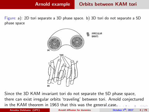
Arnold example Orbits between KAM tori
Figure: a): 2D tori separate a 3D phase space. b) 3D tori do not separate a 5Dphase space
Since the 3D KAM invariant tori do not separate the 5D phase space,there can exist irregular orbits ‘traveling’ between tori. Arnold conjecturedin the KAM theorem in 1963 that this was the general case.
Amadeu Delshams (UPC) Arnold diffusion for dummies October 4th, 2017 4 / 79

Integrable Hamiltonian sytems Action-angle variables
The unperturbed role is played by a (completely) integrable Hamiltonianwith n degrees of freedom. The Liouville–Arnold theorem establishes,under certain hypotheses, the existence on some region of the phase spaceof canonical action–angle variables (ϕ, I ) = (ϕ1, . . . , ϕn, I1, . . . , In) inTn × G ⊂ Tn × Rn, in which the Hamiltonian only depends on the actionvariables: h(I ). The associated Hamiltonian equations for a trajectory(ϕ(t), I (t)) are
ϕ = ω(I ), I = 0,
where ω = ∂Ih. Hence the dynamics is very simple: every n-dimensionaltorus I = constant is invariant, with linear flow ϕ(t) = ϕ(0) + ω(I )t, andthus all trajectories are stable. The motion on a torus is calledquasiperiodic, with associated frequencies given by the vectorω(I ) = (ω1(I ), . . . , ωn(I )).
Amadeu Delshams (UPC) Arnold diffusion for dummies October 4th, 2017 5 / 79

Integrable Hamiltonian sytems resonant and non-resonant tori
Every n-dimensional invariant torus can be non-resonant or resonant,according to whether its frequencies are rationally independent or not. Anon-resonant torus is densely filled by any of its trajectories. On the otherhand, a resonant torus is foliated into a family of lower dimensional tori.
Figure: Non-resonant 2D Torus
Amadeu Delshams (UPC) Arnold diffusion for dummies October 4th, 2017 6 / 79
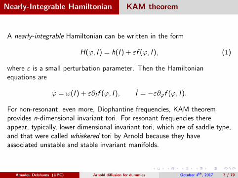
Nearly-Integrable Hamiltonian KAM theorem
A nearly-integrable Hamiltonian can be written in the form
H(ϕ, I ) = h(I ) + εf (ϕ, I ), (1)
where ε is a small perturbation parameter. Then the Hamiltonianequations are
ϕ = ω(I ) + ε∂I f (ϕ, I ), I = −ε∂ϕf (ϕ, I ).
For non-resonant, even more, Diophantine frequencies, KAM theoremprovides n-dimensional invariant tori. For resonant frequencies thereappear, typically, lower dimensional invariant tori, which are of saddle type,and that were called whiskered tori by Arnold because they haveassociated unstable and stable invariant manifolds.
Amadeu Delshams (UPC) Arnold diffusion for dummies October 4th, 2017 7 / 79

Nearly-Integrable Hamiltonian Nekhoroshev theorem
Nekhoroshev theorem, first stated in 1977, establishes Effective stabilityfor all the trajectories of a steep nearly-integrable system: For every initialcondition (ϕ(0), I (0)) one has an estimate of the type
|I (t)− I (0)| ≤ r0 εb for |t| ≤ T0 exp (ε0/ε)a .
The constants a, b > 0 are called stability exponents.If h is quasiconvex, that is, for any I ∈ G and v ∈ Rn,
Dh(I )v = 0 and v 6= 0 =⇒ v>D2h(I )v 6= 0.
a = b = 12n .
Amadeu Delshams (UPC) Arnold diffusion for dummies October 4th, 2017 8 / 79

Arnold example again Nekhoroshev estimates
H∗(q, p, ϕ, I , s,A) =1
2
(p2 + I 2
)+ A + ε(cos q− 1) (1 + µ(sinϕ+ cos s)) ,
Since h(p, I ,A) = 12
(p2 + I 2
)+ A satisfies
∣∣∣∣ D2h DhDh> 0
∣∣∣∣ = −1 < 0, one
can check that h is quasiperiodic, and a priori
|(p, I ,A)(t)− (p, I ,A)(0)| ≤ r0 ε1/6 for |t| ≤ T0 exp
(ε0/ε)1/6
.
A refinement [Poschel93, D-Gutierrez96] for orbits close to the singleresonance p = 0, using resonant normal forms, gives
|I (t)− I (0)| ≤ r0 ε1/4 for |t| ≤ T0 exp
(ε0/ε)1/4
.
Amadeu Delshams (UPC) Arnold diffusion for dummies October 4th, 2017 9 / 79

Single resonance normal form Taylor expanding in I ∈ Rn+1
For a nearly-integrable Hamiltonian with n + 1 degrees of freedom
H(ϕ, I ) = h(I ) + εf (ϕ, I ), (ϕ, I ) ∈ Tn+1 × Rn+1
Select I ∗ = 0, and assume that the associated frequency vectorλ∗ = ∂Ih(0) ∈ Rn+1 has a single resonance: 〈k∗, λ∗〉 = 0 for some0 6= k∗ ∈ Zn+1 and 〈k, λ∗〉 6= 0 for any k ∈ Zn+1 not co-linear to k∗.By a classical algebraic result, we can assume λ∗ of the form
λ∗ = (0, ω∗) ,
where ω∗ ∈ Rn is non-resonant. (In fact, we shall assume a Diophantinecondition on ω∗ to apply later on KAM theorem).The unperturbed Hamiltonian can be written (up to a constant) as:
h(I ) = 〈λ∗, I 〉+1
2〈QI , I 〉+ O3(I ).
Amadeu Delshams (UPC) Arnold diffusion for dummies October 4th, 2017 10 / 79
Single resonance normal form Split ϕ→ (q, ϕ), I → (p, I )
Replace ϕ→ (q, ϕ) and I → (p, I ), and thus split (ϕ, I ) ∈ Tn+1 ×Rn+1 as(q, p, ϕ, I ) ∈ T× R× Tn × Rn, and the matrix Q = ∂ 2
I h(0) as
∂ 2p,Ih(0) =
(β2 λ>
λ Q
),
where we have put β2 > 0 in order to fix ideas, λ ∈ Rn is a shift vector,and the new matrix Q is n × n. We will assume β = 1; this can beachieved replacing p, I by p/β, I/β (changing in this way the time scaleby a factor β), and rewriting ω∗/β, λ/β2, Q/β2 as ω∗, λ, Q respectively,and redefining also the function f .
Amadeu Delshams (UPC) Arnold diffusion for dummies October 4th, 2017 11 / 79
Single resonance normal form Designing one step
Then, we can write our Hamiltonian in the form
H(q, p, ϕ, I ) = h(p, I ) + εf (q, p, ϕ, I ),
h(p, I ) = 〈ω∗, I 〉+p2
2+ 〈λ, I 〉 p +
1
2〈QI , I 〉+ O3(p, I ).
We now perform one step of resonant normal form procedure: followingthe Lie method, we seek for functions S(q, ϕ) and R(q, p, ϕ, I ) = O(p, I )such that
S , h+ V + R = f , (2)
where V (q) is the periodic function obtained by averaging f (q, 0, ϕ, 0)with respect to the angles ϕ:
V (q) = f (q, 0, ·, 0) =1
(2π)n
∫Tn
f (q, 0, ϕ, 0)dϕ, q ∈ T.
Amadeu Delshams (UPC) Arnold diffusion for dummies October 4th, 2017 12 / 79
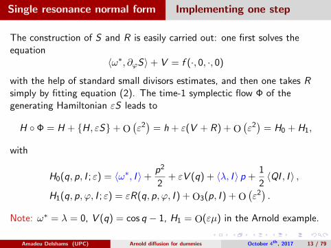
Single resonance normal form Implementing one step
The construction of S and R is easily carried out: one first solves theequation
〈ω∗, ∂ϕS〉+ V = f (·, 0, ·, 0)
with the help of standard small divisors estimates, and then one takes Rsimply by fitting equation (2). The time-1 symplectic flow Φ of thegenerating Hamiltonian εS leads to
H Φ = H + H, εS+ O(ε2)
= h + ε(V + R) + O(ε2)
= H0 + H1,
with
H0(q, p, I ; ε) = 〈ω∗, I 〉+p2
2+ εV (q) + 〈λ, I 〉 p +
1
2〈QI , I 〉 ,
H1(q, p, ϕ, I ; ε) = εR(q, p, ϕ, I ) + O3(p, I ) + O(ε2).
Note: ω∗ = λ = 0, V (q) = cos q − 1, H1 = O(εµ) in the Arnold example.
Amadeu Delshams (UPC) Arnold diffusion for dummies October 4th, 2017 13 / 79

Single resonance normal form Relation with Arnold example
This expression generalizes Arnold’s example.Concerning V , except for degenerate cases, the function V (q) will have aunique and nondegenerate maximum q0; we denote α2 = −V ′′(q0) > 0.Then, for ε > 0, the 1-degree-of-freedom Hamiltonian
P(q, p; ε) =p2
2+ εV (q),
has a saddle point in (q0, 0), with (homoclinic) separatrices. The caseε < 0 is analogous, provided one considers a minimum instead of amaximum. Then, the Hamiltonian H0 has whiskered tori with coincidentwhiskers associated to this saddle point.Note that H0 constitutes a Hamiltonian situated between the unperturbedHamiltonian h and the perturbed one H, which possesses hyperbolicinvariant tori but their whiskers still coincide.Note also that, in general, H0 is not an uncoupled Hamiltonian because ofthe coupling term 〈λ, I 〉 p.
Amadeu Delshams (UPC) Arnold diffusion for dummies October 4th, 2017 14 / 79

Single resonance normal form Introducing µ =√ε
The Lyapunov exponents of the saddle point of the “pendulum” P are±√εα, which tend to zero for ε→ 0+.
To have fixed Lyapunov exponents, we can replace p, I by√εp,√εI .
The new system is still Hamiltonian if we divide the Hamiltonian by ε(making in this way a change of time scale by a factor
√ε):
H0 = 〈ω, I 〉+p2
2+ V (q) + 〈λ, I 〉 p +
1
2〈QI , I 〉 , (3)
H1 = R(x ,√εy , ϕ,
√εI)
+1
εO3
(√εy ,√εI)
+ O (ε) = O(µ), (4)
where
ω =ω∗√ε, µ =
√ε.
Amadeu Delshams (UPC) Arnold diffusion for dummies October 4th, 2017 15 / 79

Hyperbolic Hamiltonians Regular and singular case
For ε→ 0+, the study of the Hamiltonian (3–4) is a singular perturbationproblem, due to the fast frequencies ω = ω∗/
√ε in the unperturbed
Hamiltonian H0. We are thus confronted with a singular system, oftenreferred to as weakly hyperbolic, and also called a-priori stable[Chierchia-Gallavotti94]. In fact, this case can be referred to as totallysingular, because all the frequencies are fast.
The singular problem can be avoided if one considers independentparameters, namely a fixed ε > 0 (that is, a fixed ω in (3)) and µ→ 0. Insuch a case, the system (3–4) has the property that the hyperbolicity andthe homoclinic orbits are present in the unperturbed Hamiltonian (µ = 0),and are simply perturbed for |µ| small. In this case, we are confronted witha regular or strongly hyperbolic system, or also a-priori unstable.
Amadeu Delshams (UPC) Arnold diffusion for dummies October 4th, 2017 16 / 79

Hyperbolic Hamiltonians Poincare-Arnold-Melnikov
This strategy of keeping ε > 0 fixed and letting µ→ 0 was introduced byPoincare in 1889 and followed in Arnold’s example to avoid dealing with asingular perturbation problem.
Unfortunately, the exponentially small splitting of separatrices predicted bya direct application of the Poincare-Arnold-Melnikov (PMA) method
Splitting distance = ε PMA prediction + O(εµ)
when the PMA prediction = O(e−c/ε
a)could then be justified only for µ
exponentially small in ε.
Amadeu Delshams (UPC) Arnold diffusion for dummies October 4th, 2017 17 / 79

Arnold’s proof Phase space for ε = 0
H(q, p, ϕ, I , s) =1
2p2 + ε(cos q − 1) +
1
2I 2 + εµf (q)g(ϕ, s)
f (q) = cos q − 1, g(ϕ, s) = sinϕ+ cos s,
Figure: Phase Space - Unperturbed problem for ε = 0
Amadeu Delshams (UPC) Arnold diffusion for dummies October 4th, 2017 18 / 79
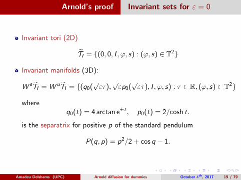
Arnold’s proof Invariant sets for ε = 0
Invariant tori (2D)
TI = (0, 0, I , ϕ, s) : (ϕ, s) ∈ T2
Invariant manifolds (3D):
W s TI = W uTI = (q0(√ετ),√εp0(√ετ), I , ϕ, s) : τ ∈ R, (ϕ, s) ∈ T2
whereq0(t) = 4 arctan e±t , p0(t) = 2/cosh t.
is the separatrix for positive p of the standard pendulum
P(q, p) = p2/2 + cos q − 1.
Amadeu Delshams (UPC) Arnold diffusion for dummies October 4th, 2017 19 / 79

Arnold’s proof Mechanism for small ε > 0
s
i
phiq
p
nhim
eps
e2
e1
e2
By the special form of the perturbation, TI persist to TIε
= TIW s TI
εand W uTI
εare ε-close to the unperturbed ones.
Using Poincare-Melnikov theory, W s TIεt W uTI
εwith an angle of
size e−π√ε/2.
Therefore W s T εIi t W uT εIi+1for |Ii − Ii+1| ≤ e−π
√ε/2 and a shadowing
(transition chain mechanism) gives the diffusion path.
Amadeu Delshams (UPC) Arnold diffusion for dummies October 4th, 2017 20 / 79

Arnold’s proof Main drawbacks of the proof
Minor 4 pages paper in Dokl. Akad. Nauk SSSR. “The details ofthe proof must be formidable, although the idea of the proofis clearly outlined.” (J. Moser in the MathSciNet review)
Fixable The perturbation maintains fixed all the invariant tori TI . Ingeneral, there appear gaps around resonant tori (rational I )which prevent W s T εIi t W uT εIi+1
because T εIi and T εIi+1are
too far. The Scattering map can fix it.
Major The exponentially small size of the splitting e−π√ε/2
computed from a direct application of the PMA method ismuch less than the Nekhoroshev estimates e−πε
1/4/2.
Major Arnold example only shows global instability along a singleresonance, where the associated normal form is integrable,but does not deal with multiple resonances, where thenormal form is not integrable.
Amadeu Delshams (UPC) Arnold diffusion for dummies October 4th, 2017 21 / 79

Arnold’s proof Main drawbacks of the proof
Exponentially small splitting of separatrices
The exponentially small splitting of separatrices was already found byPoincare in 1890, and first addressed in 1984 by Neishtadt with upperbounds using normal forms and by Lazutkin with asimptotic estimatesusing complex parameterizations of the stable and unstable invariantmanifolds.
Proofs of its asymptotic behavior for the rapidly forced pendulum or otherrapidly oscillating periodic perturbations in[D-Seara92,Gelfreich93,Fontich93-95,Sauzin95,Treschev97,D-Seara97,Gelfreich97,Baldoma-Fontich04-06,Guardia-Olive-Seara10,Baldoma-Fontich-Guardia-Seara12].
For maps, upper exponentially small estimates in [Fontich-Simo90] andasymptotic estimates in[D-Ramırez-Ros98-99,Simo-Vieiro09,Martın-Sauzin-Seara11].
Amadeu Delshams (UPC) Arnold diffusion for dummies October 4th, 2017 22 / 79

Arnold’s proof Main drawbacks of the proof
Exponentially small splitting of separatrices
In the rapidly quasiperiodically forced pendulum, the role of the arithmeticproperties was detected in [Sim94], and established in[D-Gelfreich-Seara-Jorba97].
For n-dimensional whiskered tori of a Hamiltonian with n + 1 degrees offreedom, the splitting potential and Melnikov potential were introduced[Eliasson94,D-Gutierrez00], sharp exponentially small upper bounds weregiven in [D-Gutierrez-Seara04], and asymptotic estimates in[Lochak-Marco-Sauzin03,D-Gutierrez04,D-GonchenkoGutierrez14-16].
The multidimensional separatrix map introduced by Treschev in 2002requires more study.
Amadeu Delshams (UPC) Arnold diffusion for dummies October 4th, 2017 23 / 79

A priori unstable systems A model
We consider a 2π-periodic in time perturbation of a pendulum and a rotordescribed by the non-autonomous Hamiltonian,
Hε(p, q, I , ϕ, t) = H0(p, q, I ) + εh(p, q, I , ϕ, t; ε)= P±(p, q) + 1
2 I2 + εh(p, q, I , ϕ, t; ε)
(5)
where (p, q, I , ϕ, t) ∈ (R× T)2 × T and
P±(p, q) = ±(
1
2p2 + V (q)
)(6)
and V (q) is a 2π-periodic function. We will refer to P±(p, q) as thependulum.Note. This model just comes from a normal form around a singleresonance of a nearly integrable Hamiltonian. The perturbation is arbitrary.
Amadeu Delshams (UPC) Arnold diffusion for dummies October 4th, 2017 24 / 79

A priori unstable systems Global instability
Theorem (D-Llave-Seara06)
Consider the Hamiltonian (5) where V and h are uniformly Cr+2 forr ≥ r0, sufficiently large. Assume also that
H1 The potential V : T→ R has a unique global maximum at q = 0which is non-degenerate. Denote by (q0(t), p0(t)) an orbit of thependulum P±(p, q) homoclinic to (0, 0).
H2 The Melnikov potential, associated to h (and to the homoclinic orbit(p0, q0)):
L(I , ϕ, s) = −∫ +∞
−∞(h(p0(σ), q0(σ), I , ϕ+ Iσ, s + σ; 0)
−h(0, 0, I , ϕ+ Iσ, s + σ; 0))dσ(7)
satisfies concrete non-degeneracy conditions.
H3 The perturbation term h satisfies concrete non-degeneracy conditions.
Amadeu Delshams (UPC) Arnold diffusion for dummies October 4th, 2017 25 / 79

A priori unstable systems Global instability
Then, there is ε∗ > 0 such that for 0 < ε < ε∗, and for any interval [I ∗−, I∗+],
there exists a trajectory x(t) of the system (5) such that for some T > 0,
I (x(0)) ≤ I ∗−; I (x(T )) ≥ I ∗+.
Remark Arbitrary excursions in the I variable can also be realized.
Amadeu Delshams (UPC) Arnold diffusion for dummies October 4th, 2017 26 / 79
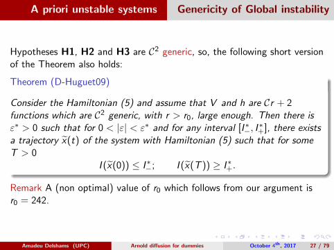
A priori unstable systems Genericity of Global instability
Hypotheses H1, H2 and H3 are C2 generic, so, the following short versionof the Theorem also holds:
Theorem (D-Huguet09)
Consider the Hamiltonian (5) and assume that V and h are Cr + 2functions which are C2 generic, with r > r0, large enough. Then there isε∗ > 0 such that for 0 < |ε| < ε∗ and for any interval [I ∗−, I
∗+], there exists
a trajectory x(t) of the system with Hamiltonian (5) such that for someT > 0
I (x(0)) ≤ I ∗−; I (x(T )) ≥ I ∗+.
Remark A (non optimal) value of r0 which follows from our argument isr0 = 242.
Amadeu Delshams (UPC) Arnold diffusion for dummies October 4th, 2017 27 / 79

A priori unstable systems A multidimensional model
Consider a periodic in time perturbation of n pendula and a d-dimensionalrotor described by the non-autonomous Hamiltonian,
H(p, q, I , ϕ, t, ε) = P(p, q) + h(I ) + εQ(p, q, I , ϕ, t, ε), (8)
with P(p, q) =∑n
j=1 Pj(pj , qj), Pj(pj , qj) = ±(
12p
2j + Vj(qj)
), where
I ∈ I ⊂ Rd , ϕ ∈ Td , I an open set, p, q ∈ Rn, t ∈ T1, and Pj(pj , qj) is apendulum for the saddle variables pj , qj . For ε = 0, the d-dimensionalaction I remains constant. Under similar hypotheses as for n = d = 1,
Theorem (D-Llave-Seara12)
For every δ > 0, there exists ε0 > 0, such that for every 0 < |ε| < ε0,given I± ∈ I,there exists a solution x(t) of (8) and T > 0, such that
|I (x(0))− I−| ≤ Cδ and |I (x(T ))− I+| ≤ Cδ (9)
Amadeu Delshams (UPC) Arnold diffusion for dummies October 4th, 2017 28 / 79

A priori unstable systems A multidimensional model
One can forget about δ and prescribe arbitrary paths on a set I∗.This set I∗ is described precisely in the course of the proof, and isdetermined by the non-degeneracy assumptions. The main idea isthat I∗ is obtained from the domain of definition, just eliminatingsome sets of codimension 2, like double resonances, from the open setwhere the intersection of stable and unstable manifolds of a normallyhyperbolic invariant manifold is transversal.
Codimension 2 objects do not separate the regions and can becontoured so that they do not obstruct the change along the paths. Itseems that such contouring trajectories close to double resonances areinferred from some movies related to numerical experiments in(Gelfreich-Simo-Vieiro 13)
Amadeu Delshams (UPC) Arnold diffusion for dummies October 4th, 2017 29 / 79

A priori unstable systems A multidimensional model
Amadeu Delshams (UPC) Arnold diffusion for dummies October 4th, 2017 30 / 79

Other contributions
This problem of instability, also called Arnold diffusion, was posed first byArnold in 1964, and there have been some other contributions, usinggeometrical or variational methods:[Lochak92], [Chierchia-Gallavotti94-98], [Bessi-Chierchia-Valdinoci01][Berti-Biasco-Bolle03], [Marco-Sauzin03], [Mather04], [Cheng-Yan04],[Gidea-Llave06], [Piftankin-Treschev07], [Kaloshin-Levi08], [ChengY09],[Bernard-Kaloshin-Zhang11], [Zhang11], [Mather12], [Treschev12],[Gelfreich-Simo-Vieiro13], [GelfreichT14], [Gidea-Llave-Seara14],[Kaloshin-Zhang15], [Lazzarini-Marco-SauzinS15],[Davletshin-Treschev16], [Marco16], [Gidea-Marco17], [Cheng17].

A priori unstable systems Idea of the proof
The main idea of the proof is to use the two (or more) dynamics on Λ.
Find a big invariant saddle object: a NHIM (normally hyperbolicinvariant manifold: a global version of a center manifold) Λ withtransverse associated stable and unstable manifolds along somehomoclinic manifold Γ: Wu(Λ) tΓ Ws(Λ).
Compute the invariant objects (typically tori T ) which may preventinstability for the inner dynamics of the NHIM.
Compute an scattering map S = SΓ : H− ⊂ Λ→ H+ ⊂ Λ on theNHIM associated to Γ and consider it as an outer dynamics on theNHIM (a second dynamics on Γ).
Check that S(TIi ) t TIi+1for a sequence of tori TIiNi=1 with
|IN − I1| = O(1), and construct a transition chain of whiskered tori,i.e. Wu(TIi ) tWs(TIi+1
).
Standard shadowing methods provide an orbit that follows closely thetransition chain.
Amadeu Delshams (UPC) Arnold diffusion for dummies October 4th, 2017 32 / 79

Proof in a concrete example The result
Consider a pendulum and a rotor plus a time periodic perturbationdepending on two harmonics in the variables (ϕ, s):
Hε(p, q, I , ϕ, t) = ±(p2
2+ cos q − 1
)+
I 2
2+ εh(q, ϕ, s) (10)
h(q, ϕ, s) = f (q)g(ϕ, s),
f (q) = cos q, g(ϕ, s) = a1 cos(k1ϕ+ l1s) + a2 cos(k2ϕ+ l2s),(11)
with k1, k2, l1, l2 ∈ Z.
Theorem
Assume that a1a2 6= 0 and∣∣∣k1 k2l1 l2
∣∣∣ 6= 0 in (10)-(11). Then, for any I ∗ > 0,
there exists ε∗ = ε∗(I ∗, a1, a2) > 0 such that for any ε, 0 < ε < ε∗, thereexists a trajectory (p(t), q(t), I (t), ϕ(t)) such that for some T > 0
I (0) ≤ −I ∗ < I ∗ ≤ I (T ).
Amadeu Delshams (UPC) Arnold diffusion for dummies October 4th, 2017 33 / 79

Proof in a concrete example The two dynamics in NHIM
We have two important dynamics associated to the system: the inner andthe outer dynamics.
Λ = (0, 0, I , ϕ, s); I ∈ [−I ∗, I ∗] , (ϕ, s) ∈ T2.
is a 3D Normally Hyperbolic Invariant Manifold (NHIM) with associated4D stable W s
ε (Λ) and unstable W uε (Λ) invariant manifolds.
The inner dynamics is the dynamics restricted to Λ. (Inner map)
The outer dynamics is the dynamics restricted to its invariantmanifolds. (Scattering map)
Remark: for simplicity, in our case Λ = Λε .
Amadeu Delshams (UPC) Arnold diffusion for dummies October 4th, 2017 34 / 79

Proof in a concrete example Scattering map
Let Λ be a NHIM with invariant manifolds intersecting transversally alonga homoclinic manifold Γ. A scattering map is a map S defined byS(x−) = x+ if there exists z ∈ Γ satisfying
|φεt (z)− φεt (x∓)| −→ 0 as t −→ ∓∞
that is, W uε (x−) intersects transversally W s
ε (x+) in z .
Amadeu Delshams (UPC) Arnold diffusion for dummies October 4th, 2017 35 / 79

Proof in a concrete example Reduced Poincare L∗(I , θ)
S is symplectic and exact (Delshams -de la Llave - Seara 2008) and takes theform:
Sε(I , ϕ, s) =
(I + ε
∂L∗
∂θ(I , θ) +O(ε2), θ − ε ∂L
∗
∂I(I , θ) +O(ε2), s
),
where θ = ϕ− Is and L∗(I , θ) is the Reduced Poincare function, or more simplyin the variables (I , θ):
Sε(I , θ) =
(I + ε
∂L∗
∂θ(I , θ) +O(ε2), θ − ε ∂L
∗
∂I(I , θ) +O(ε2)
),
The variable s remains fixed under Sε: it plays the role of a parameter
Up to first order in ε, Sε is the −ε-time flow of the Hamiltonian L∗(I , θ)
The scattering map jumps O(ε) distances along the level curves of L∗(I , θ)
Amadeu Delshams (UPC) Arnold diffusion for dummies October 4th, 2017 36 / 79
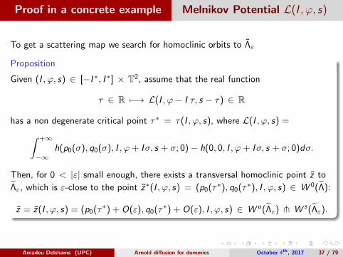
Proof in a concrete example Melnikov Potential L(I , ϕ, s)
To get a scattering map we search for homoclinic orbits to Λε
Proposition
Given (I , ϕ, s) ∈ [−I ∗, I ∗] × T2, assume that the real function
τ ∈ R 7−→ L(I , ϕ− I τ, s − τ) ∈ R
has a non degenerate critical point τ∗ = τ(I , ϕ, s), where L(I , ϕ, s) =∫ +∞
−∞h(p0(σ), q0(σ), I , ϕ+ Iσ, s + σ; 0)− h(0, 0, I , ϕ+ Iσ, s + σ; 0)dσ.
Then, for 0 < |ε| small enough, there exists a transversal homoclinic point z to
Λε, which is ε-close to the point z∗(I , ϕ, s) = (p0(τ∗), q0(τ∗), I , ϕ, s) ∈ W 0(Λ):
z = z(I , ϕ, s) = (p0(τ∗) + O(ε), q0(τ∗) + O(ε), I , ϕ, s) ∈ W u(Λε) t W s(Λε).
Amadeu Delshams (UPC) Arnold diffusion for dummies October 4th, 2017 37 / 79

Proof in a concrete example L(I , ϕ, s) and L∗(I , θ)
In our model the perturbation is
h(p, q, I , ϕ, s) = cos q (a0 cos(k1ϕ+ l1s) + a1 cos(k2ϕ+ l2s))
and the Melnikov potential becomes
L(I , ϕ, s) = A0(I ) cos(k1ϕ+ l1s) + A1(I ) cos(k2ϕ+ l2s),
where A0(I ) =2π (k1I + l1) a0
sinh( (k1I+l1)π2 )
and A1 =2 (k2I + l2)π a1
sinh( (k2I+l2)π2 )
.
Definition
The Reduced Poincare function is
L∗(I , θ) = L(I , ϕ− I τ∗(I , ϕ, s), s − τ∗(I , ϕ, s)),
where θ = ϕ− I s.
Amadeu Delshams (UPC) Arnold diffusion for dummies October 4th, 2017 38 / 79

Proof in a concrete example Plot of L(I , ϕ, s)
Figure: The Melnikov Potential, µ = a0/a1 = 0.6, I = 1, k1 = l2 = 1 andk2 = l1 = 0.
Amadeu Delshams (UPC) Arnold diffusion for dummies October 4th, 2017 39 / 79

Proof in a concrete example The function τ ∗
We look for τ∗ such that ∂L∂τ (I , ϕ− I τ∗, s − τ∗) = 0.
Different view-points for τ∗ = τ∗(I , ϕ, s)
Look for critical points of L on the straight lineR(I , ϕ, s) = (ϕ− I τ, s − τ), τ ∈ R.Look for intersections between R(I , ϕ, s) = (ϕ− I τ, s − τ), τ ∈ Rand a crest which is a curve of equation
∂L∂τ
(I , ϕ− I τ, s − τ)|τ=0 = 0.
Amadeu Delshams (UPC) Arnold diffusion for dummies October 4th, 2017 40 / 79
Proof in a concrete example Crests
Definition - Crests (Delshams-Huguet 2011)
For each I , we call crest C(I ) the set of curves in the variables (ϕ, s) of equation
I∂L∂ϕ
(I , ϕ, s) +∂L∂s
(I , ϕ, s) = 0. (12)
which in our case can be rewritten as
µα(I ) sinϕ+ sin s = 0, with α(I ) =sinh(π
2) I 2
sinh(π I2
), µ =
a10
a01. (13)
For any I , the critical points of the Melnikov potential L(I , ·, ·) ((0, 0), (0, π),(π, 0) and (π, π): one maximum, one minimum point and two saddle points)always belong to the crest C(I ).
L∗(I , θ) is nothing else but L evaluated on the crest C(I ).
θ = ϕ− Is is constant on the straight line R(I , ϕ, s)
Amadeu Delshams (UPC) Arnold diffusion for dummies October 4th, 2017 41 / 79

Proof in a concrete example Geometry of a crest
Figure: Level curves of L for µ = a0/a1 = 0.5, I = 1.2, k1 = l2 = 1 andk2 = l1 = 0.
Amadeu Delshams (UPC) Arnold diffusion for dummies October 4th, 2017 42 / 79

Proof in a concrete example Geometry of a crest
Understanding the behavior of the crests
⇓Understanding the behavior of the Reduced Poincare function
⇓Understanding the Scattering map
Amadeu Delshams (UPC) Arnold diffusion for dummies October 4th, 2017 43 / 79

Proof in a concrete example Reduction to two cases
We only need to study two cases:
The first (easier) case [D-Schaefer 17]
h(q, ϕ, s) = cos q (a0 cosϕ+ a1 cos s)
The second case [D-Schaefer 17]
h(q, ϕ, s) = cos q (a0 cosϕ+ a1 cos(ϕ− s))
Each case has its own characteristics and together are enough tounderstand the general case.We present just some highlights about each case.
Amadeu Delshams (UPC) Arnold diffusion for dummies October 4th, 2017 44 / 79
k1 = l2 = 1 and k2 = l1 = 0 Highways
Definition: Highways
Highways are the level curves of L∗ such that
L∗(I , θ) =2πa0
sinh(π/2).
The highways are “vertical” in the variables (ϕ, s)
We always have a pair of highways. One goes up, the other goesdown (this depends on the sign of µ = a0/a1)
The highways give rise to fast diffusing pseudo-orbits
Amadeu Delshams (UPC) Arnold diffusion for dummies October 4th, 2017 45 / 79

k1 = l2 = 1 and k2 = l1 = 0 Plot of highways
Figure: The scattering map jumps O(ε) distances along the level curves ofL∗(I , θ)
Amadeu Delshams (UPC) Arnold diffusion for dummies October 4th, 2017 46 / 79

k1 = l2 = 1 and k2 = l1 = 0 0 < |µ| < 0.97
For |µα(I )| < 1, there are two crests CM,m(I ) parameterized by:
s = ξM(I , ϕ) = − arcsin(µα(I ) sinϕ) mod 2π (14)
ξm(I , ϕ) = arcsin(µα(I ) sinϕ) + π mod 2π
They are “horizontal” crests
Amadeu Delshams (UPC) Arnold diffusion for dummies October 4th, 2017 47 / 79

k1 = l2 = 1 and k2 = l1 = 0 0 < |µ| < 0.625
For each I , the line R(I , ϕ, s) and the crest CM,m(I ) have only one intersectionpoint.
The scattering map SM associated to the intersections between CM(I ) andR(I , ϕ, s) is well defined for any ϕ ∈ T. Analogously for Sm, changing M to m. Inthe variables (I , θ = ϕ− Is), both scattering maps SM, Sm are globally well defined.
(a) Level curves of L∗M(I , θ) (b) Level curves of L∗m(I , θ)
Amadeu Delshams (UPC) Arnold diffusion for dummies October 4th, 2017 48 / 79

k1 = l2 = 1 and k2 = l1 = 0 0.625 < |µ|
There are tangencies between CM,m(I , ϕ) and R(I , ϕ, s). For some value of(I , ϕ, s), there are 3 points in R(I , ϕ, s) ∩ CM,m(I ).
This implies that there are 3 scattering maps associated to each crest withdifferent domains.(Multiple Scattering maps)
Amadeu Delshams (UPC) Arnold diffusion for dummies October 4th, 2017 49 / 79

k1 = l2 = 1 and k2 = l1 = 0 0.625 < |µ|
(c) The three types of level curves. (d) Zoom where the scattering mapsare different
Figure: Level curves of L∗M(I , θ), L∗(1)M (I , θ) and L∗(2)
M (I , θ)
Amadeu Delshams (UPC) Arnold diffusion for dummies October 4th, 2017 50 / 79

k1 = l2 = 1 and k2 = l1 = 0 0.97 < |µ|
For some values of I , |µα(I )| > 1, the two crests CM,m are parameterized by:
ϕ = ηM(I , s) = − arcsin(µα(I ) sin s) mod 2π (15)
ηm(I , s) = arcsin(µα(I ) sin s) + π mod 2π
They are “vertical” crests
Amadeu Delshams (UPC) Arnold diffusion for dummies October 4th, 2017 51 / 79

k1 = l2 = 1 and k2 = l1 = 0 0.97 < |µ|
For the values of I and when horizontal crests become vertical, it is notalways possible to prolong in a continuous way the scattering maps, so thedomain of the scattering map has to be restricted.
Figure: The level curves of L∗M(I , θ), µ = 1.5.
In green, the region where the scattering map SM is not defined.
Amadeu Delshams (UPC) Arnold diffusion for dummies October 4th, 2017 52 / 79

k1 = l2 = 1 and k2 = l1 = 0 An example of pseudo-orbit
Figure: In red: Inner map, blue: Scattering map, black: Highways
Amadeu Delshams (UPC) Arnold diffusion for dummies October 4th, 2017 53 / 79
k1 = l2 = 1 and k2 = l1 = 0 Time of diffusion
An estimate of the total time of diffusion between −I ∗ and I ∗, along the highway, is
Td =Ts
ε
[2 log
(C
ε
)+O(εb)
], for ε→ 0, where 0 < b < 1,
with
Ts = Ts(I∗, a10, a01) =
∫ I∗
0
− sinh(πI/2)
πa10I sinψh(I )dI ,
where ψh = θ − Iτ∗(I , θ) is the parameterization of the highway L∗(I , ψh) = A00 + A01,and
C = C(I ∗, a10, a01) = 16 |a10|
(1 +
1.465√1− µ2A2
)
where A = maxI∈[0,I∗] α(I ), with α(I ) =sinh( π
2) I 2
sinh( π I2
)and µ = a10/a01.
Note: This estimate quantifies the general optimal diffusion estimate O(
1
εlog
1
ε
)of
[Berti-Biasco-Bolle 2003], [Cresson-Guillet 2003] and [Treschev 2004).
Amadeu Delshams (UPC) Arnold diffusion for dummies October 4th, 2017 54 / 79

k1 = k2 = 1, l2 = −1 and l1 = 0 The second case
Main differences between the first and the second case
In the second case:
There are no Highways.
For any value of µ = a0/a1 is possible to find Ih and Iv such that forI = Ih the crests are horizontal and for I = Iv the crests are vertical.
For any value of µ there exists I such that the crests and R(I , ϕ, s)are tangent.
Amadeu Delshams (UPC) Arnold diffusion for dummies October 4th, 2017 55 / 79

k1 = k2 = 1, l2 = −1 and l1 = 0 Scattering maps for one crest
The choice of the concrete curve of the crest and therefore of τ∗(I , θ) isvery important and useful.
Figure: The “lower” crest Figure: The “upper” crest
Green zones: I increases under the scattering map.Red zones: I decreases under the scattering map.
Amadeu Delshams (UPC) Arnold diffusion for dummies October 4th, 2017 56 / 79
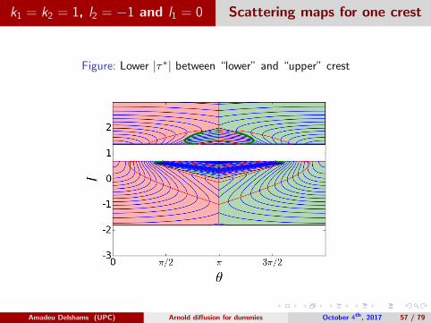
k1 = k2 = 1, l2 = −1 and l1 = 0 Scattering maps for one crest
Figure: Lower |τ∗| between “lower” and “upper” crest
Amadeu Delshams (UPC) Arnold diffusion for dummies October 4th, 2017 57 / 79

k1 = k2 = 1, l2 = −1 and l1 = 0 a non-smooth scattering map
In this picture we show a combination of 6 scattering maps.
Amadeu Delshams (UPC) Arnold diffusion for dummies October 4th, 2017 58 / 79
3 + 1/2 degrees of freedom A model
H(I1, I2, ϕ1, ϕ2, p, q, t, ε) = ±(p2
2+ cos q − 1
)+ h(I1, I2) + ε cos q g(ϕ1, ϕ2, t),
where
h(I1, I2) = Ω1I 21
2+ Ω2
I 22
2
andg(ϕ1, ϕ2, t) = a1 cosϕ1 + a2 cosϕ2 + a3 cos(ϕ1 + ϕ2 − t).
Under general conditions for a1, a2, a3,Ω1,Ω2, global instability was established in
[D-Llave-Seara 2016]
Amadeu Delshams (UPC) Arnold diffusion for dummies October 4th, 2017 59 / 79

3 + 1/2 degrees of freedom Melnikov potential
In this case, the Melnikov potential is
L(I , ϕ− ωτ) =3∑
i=1
Ai cos(ϕi − ωiτ),
where ϕ = (ϕ1, ϕ2, ϕ3), ω = (ω1, ω2, ω3), ϕ3 = ϕ1 + ϕ2 − s,
Ai =2πωi
sinh(π ωi2 )
ai ,
and
ω1 = Ω1I1 ω2 = Ω2I2 ω3 = ω1 + ω2 − 1.
Remark: The reduced Poincare function L∗(I , θ) can be defined but theassociated Hamiltonian vector field is no longer integrable
Amadeu Delshams (UPC) Arnold diffusion for dummies October 4th, 2017 60 / 79

3 + 1/2 degrees of freedom Example of crests
Figure: Horizontal crests:µ1 = µ2 = 0.48,ω1 = ω2 = 1.219.
Figure: Crests with holes : µ1 = 0.7,µ2 = 0.6,ω1 = ω2 = 1.219.
Amadeu Delshams (UPC) Arnold diffusion for dummies October 4th, 2017 61 / 79

3 + 1/2 degrees of freedom Behavior of the crests
Figure: ω1 = ω2 = 1.219Figure: µ1 = µ2 = 1.2
Pink: Surface with holes, white: horizontal surfaces s(ϕ1, ϕ2), purple: vertical surfaces
ϕ1(ϕ2, s), green: vertical surfaces ϕ2(ϕ1, s).
Amadeu Delshams (UPC) Arnold diffusion for dummies October 4th, 2017 62 / 79

A priori chaotic systems geodesic flow
(Quasi)-periodic perturbations of geodesic flows
Theorem ([D-Llave-Seara06])
Let M be a n-dimensional manifold, g a Cr metric on it (r sufficientlylarge). Assume:
H1 There exists a closed geodesic “Λ” such that its correspondingperiodic orbit Λ under the geodesic flow is hyperbolic.
H2 There exists another geodesic “γ” such that γ is a transversalhomoclinic orbit to Λ.That is, γ is contained in the intersection of the stable and unstablemanifolds of Λ, W s
Λ, W u
Λ, in the unit tangent bundle.
Moreover, we assume that the intersection of the stable and unstablemanifolds of Λ is transversal along γ. That is,
Tγ(t)WsΛ
+ Tγ(t)WuΛ
= Tγ(t)S1M, t ∈ R.
Amadeu Delshams (UPC) Arnold diffusion for dummies October 4th, 2017 63 / 79

A priori chaotic systems geodesic flow
Abundance of Hypoteses H1, H2
Hipotheses H1, H2 are abundant:
They are generic on T2 [Morse24], [Hedlund32], [Mather94].
They hold on any closed surface of genus bigger or equal than 2, ifr ≥ 2 + δ, δ > 0. [Katok82]).
They are generic in the C2 topology for any closed surface[Contreras-Paternain02].
Amadeu Delshams (UPC) Arnold diffusion for dummies October 4th, 2017 64 / 79

A priori chaotic systems geodesic flow
(Quasi)-periodic perturbations of geodesic flows
Let ν ∈ Rd be Diophantine, r ∈ N be sufficiently large (depending on τ ,the Diophantine exponent of ν).Let g be a Cr metric on a compact manifold M, verifying hypotheses H1,H2, and U : M × Td → R a generic Cr function.Consider the time dependent Lagrangian
L(q, q, νt) =1
2gq(q, q)− U(q, νt), (16)
where gq denotes the metric in TqM.Then, the Euler-Lagrange equation of L has a solution q(t) whose energy
E (t) =1
2gq(q(t), q(t)) + U(q(t), νt),
tends to infinity as t →∞.
Amadeu Delshams (UPC) Arnold diffusion for dummies October 4th, 2017 65 / 79

A priori chaotic systems ERTBP
(Planar) elliptic restricted three body problem (ERTBP)
Consider the motion of a particle q with zero mass (comet) under theattraction of two particles q1 (Sun, with mass 1− µ) and q2 (Jupiter,with mass µ), called primaries, which move in elliptic orbits witheccentricity e0 around their center of mass.
The motion of q is described by a time-periodic Hamiltonian system,with 2 and 1/2 degrees of freedom, with Hamiltonian
H(q, p, t; e0, µ) =p2
2− (1− µ)
|q − q1(t, e0)|− µ
|q − q2(t, e0)|.
We consider the motion of the particle q (comet) when it movesoutside of the orbit of the primaries along nearly parabolic orbits.
Parameters: 0 < µ < 1, e0 ≥ 0, small.
Amadeu Delshams (UPC) Arnold diffusion for dummies October 4th, 2017 66 / 79

A priori chaotic systems ERTBP
The two body problem: Sun-comet for µ = 0
When µ = 0, the Sun is fixed at the origin: q1(t, e0) = 0
The Sun q1 and the comet q form the two-body problem.
In polar coordinates: q = (r cosα, r sinα), α ∈ T, r ≥ 0, theHamiltonian of the two body problem becomes
H0(r ,Pr , α,G ) =P2r
2+
G 2
2r2− 1
r,
H0 is the energy and G = Pα is the angular momentum.
H0 and G are both first integrals of motion.
If H0 = h < 0, motions are elliptic with semi-major axis a = 1/(−2h)and eccentricity e =
√1 + 2hG 2.
If h = 0 (which corresponds to e = 1) the motion is parabolic.
The two-body problem is integrable.
Amadeu Delshams (UPC) Arnold diffusion for dummies October 4th, 2017 67 / 79

A priori chaotic systems ERTBP
Diffusion of the angular momentum G
In the elliptic restricted three body (ERTBP) problem we want to see thatthe angular momentum of the comet G (t) can have large changes whenthe eccentricity e0 > 0 and µ > 0 are small enough:
Theorem (D-Kaloshin-Rosa-Seara12)
Given any G1,G2 1, there exist trajectories of the ERTBP whoseangular momentum satisfies, for some T > 0:
G (0) < G1 G (T ) > G2
Proven for 0 < µ e0 1 and any 1 G1,G2 1/e0.Likely (need still some work) for any 0 < e0 < 1 and 0 < µ 1.Remark Two different scattering maps are used in the construction of thediffusing trajectories.
Amadeu Delshams (UPC) Arnold diffusion for dummies October 4th, 2017 68 / 79

spatial RTBP close to L1
Arnold’s mechanism of diffusion in the spatial RTBP
Model:
The spatial circular restricted three-body problem: an infinitesimalmass moves in space under the gravitational influence of two massivebodies (primaries) describing circular orbits, without exerting anyinfluence on themFocus on the dynamics near L1, the libration point between theprimaries – center×center×saddle
Results:There exist trajectories that change the out-of-plane amplitude (w.r. tothe ecliptic) of an orbit near L1 by a ‘significant amount’, via theArnold mechanism of instability
abstract theorem – if certain conditions hold true then the existence ofdrift trajectories followsverification of conditions – some analytical, some numerical
Related works [Sama,2004],[Terra,Simo,de Sousa Silva,2014]
Amadeu Delshams (UPC) Arnold diffusion for dummies October 4th, 2017 69 / 79

spatial RTBP close to L1
Introduction
Method:
There exists a normally hyperbolic invariant three-sphereWe construct orbits that alternatively follow segments of homoclinictrajectories (outer dynamics) with segments of trajectories restricted tothe three-sphere (inner dynamics), thus mimicking Arnold’s instabilitymechanism of transition tori1
However, we use only coarse information on the inner dynamics(Poincare recurrence theorem), no detailed information on the invariantobjects (KAM tori, Aubry-Mather sets, etc.)We use a geometric method that allows for explicit construction ofdrifting trajectories under milder conditions on the dynamics (comparedto variational methods)This is a general strategy
1Our model is not a small perturbation of an integrable systemAmadeu Delshams (UPC) Arnold diffusion for dummies October 4th, 2017 70 / 79

spatial RTBP close to L1
Reference Problem: 3D Circular RTBP
The Restricted Three Body Problem (RTBP) defined as
X − 2Y = ΩX ,
Y + 2X = ΩY ,
Z = ΩZ ,
where
Ω =1
2(X 2 + Y 2) +
1− µr1
+µ
r2+
1
2µ(1− µ),
r21 = (X − µ)2 + Y 2 + Z 2,
r22 = (X − µ+ 1)2 + Y 2 + Z 2.
Amadeu Delshams (UPC) Arnold diffusion for dummies October 4th, 2017 71 / 79

spatial RTBP close to L1
Libration Points
X -coordinate of L1 is
X1 = −1 +(µ
3
)1/3− 1
3
(µ3
)2/3+ Oµ.
In the Sun-Earth system,
dist L1Earth ' 1.5 · 106 km, dist SunEarth ' 150 · 106 km.Amadeu Delshams (UPC) Arnold diffusion for dummies October 4th, 2017 72 / 79
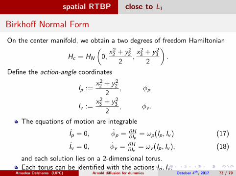
spatial RTBP close to L1
Birkhoff Normal Form
On the center manifold, we obtain a two degrees of freedom Hamiltonian
Hc = HN
(0,
x22 + y2
2
2,x2
3 + y23
2
).
Define the action-angle coordinates
Ip :=x2
2 + y22
2, φp
Iv :=x2
3 + y23
2, φv .
The equations of motion are integrable
Ip = 0, φp = ∂H∂Ip
= ωp(Ip, Iv ) (17)
Iv = 0, φv = ∂H∂Iv
= ωv (Ip, Iv ), (18)
and each solution lies on a 2-dimensional torus.Each torus can be identified with the actions Ip, Iv .
Amadeu Delshams (UPC) Arnold diffusion for dummies October 4th, 2017 73 / 79

spatial RTBP close to L1
Family of Invariant Tori
Let us fix the energy level to H(0, Ip, Iv ) = h, withH(L1) ≤ h ≤ H(halo).Then we obtain a one-parameter family of invariant tori, parametrizedby the vertical action Iv . Iv=0.00
Iv=0.05Iv=0.95Iv=1.00
-0.992-0.9915
-0.991-0.9905
-0.99-0.9895
-0.989-0.9885
X -0.005-0.004
-0.003-0.002
-0.0010
0.0010.002
0.0030.004
0.005
Y
-0.005-0.004-0.003-0.002-0.001
00.0010.0020.0030.0040.005
Z
Figure: Low energy level C = 3.00088
Amadeu Delshams (UPC) Arnold diffusion for dummies October 4th, 2017 74 / 79

spatial RTBP close to L1
Family of Invariant Tori
Let us fix the energy level to H(0, Ip, Iv ) = h, withH(L1) ≤ h ≤ H(halo).Then we obtain a one-parameter family of invariant tori, parametrizedby the vertical action Iv . Iv=0.00
Iv=0.05Iv=0.95Iv=1.00
-0.992-0.9915
-0.991-0.9905
-0.99-0.9895
-0.989-0.9885
X -0.005-0.004
-0.003-0.002
-0.001 0
0.001 0.002
0.003 0.004
0.005
Y
-0.005
-0.004
-0.003
-0.002
-0.001
0
0.001
0.002
0.003
0.004
0.005
Z
Figure: High energy level C = 3.00083
Amadeu Delshams (UPC) Arnold diffusion for dummies October 4th, 2017 74 / 79

spatial RTBP close to L1
Transition Matrix
0
0.2
0.4
0.6
0.8
1
0 0.2 0.4 0.6 0.8 1
I v(d
estin
atio
n to
rus)
Iv (source torus)
Figure: Low energy level C = 3.00087
Amadeu Delshams (UPC) Arnold diffusion for dummies October 4th, 2017 75 / 79

spatial RTBP close to L1
Transition Matrix
0
0.2
0.4
0.6
0.8
1
0 0.2 0.4 0.6 0.8 1
I v(d
estin
atio
n to
rus)
Iv (source torus)
Figure: High energy level C = 3.00083
Amadeu Delshams (UPC) Arnold diffusion for dummies October 4th, 2017 75 / 79

spatial RTBP close to L1
Main theoretical result (D-Gidea-Roldan 17)
Main Theorem. Given δ > 0.Assume ∃ LΣ
Ijj=0,N level sets of Iv , with 0 < Ij < Imax , and δj with
0 < δj < δ/2, s.t., for each j = 0, . . . ,N − 1:
(i) ∃ scattering map σΣi(j) and pt. (Ij , φj) ∈ LΣ
Ijs.t.
Bδj (Ij , φj) ⊂ domσΣi(j),
(ii) ∃kj > 0 s.t. int[F kj σΣi(j)(Bδj (Ij , φj))] ⊇ Bδj+1
(Ij+1, φj+1)
Then ∃ an orbit zj of F in Σ, j = 0, . . . ,N, and a sequence of positiveintegers nj > 0, j = 0, . . . ,N − 1, such that zj+1 = F nj (zj) and
d(zj ,LΣIj
) < δ/2, for all j = 0, . . . ,N. (19)
Consequently, there exist a trajectory Φt(z) of the Hamiltonian flow, and afinite sequence of times 0 = t0 < t1 < t2 < . . . < tN , such that
d(Φtj (z),LIj ) < δ. (20)
Amadeu Delshams (UPC) Arnold diffusion for dummies October 4th, 2017 76 / 79

spatial RTBP close to L1
Main theoretical result
1
2 3
4 5
6
0 1 2 3 4 5 6phi_v
0
0.1
0.2
0.3
0.4
0.5
0.6
0.7
0.8
I_v
Amadeu Delshams (UPC) Arnold diffusion for dummies October 4th, 2017 77 / 79

spatial RTBP Future work
Try to find drift orbits by constructing pseudo-orbits consisting ofsuccessive applications of several scattering maps
Obtain theoretical results, using Hill locally and Kepler globally
Add time dependent perturbation—elliptic orbit of Jupiter—andderive the existence of drift orbits
Amadeu Delshams (UPC) Arnold diffusion for dummies October 4th, 2017 78 / 79


