2D discontinuous piecewise linear map: Emergence of fashion cycles

Laura Gardinia, Iryna Sushkob, Kiminori MatsuyamacaDept of Economics, Society and Politics, University of Urbino, Italy

bInstitute of Mathematics, NASU, UkrainecDept of Economics, Northwestern University, USA

Abstract

We consider a discrete-time version of the continuous-time fashion cycle model introduced in Matsuyama,1992. Its dynamics are de�ned by a 2D discontinuous piecewise linear map depending on three parameters.In the parameter space of the map periodicity regions associated with attracting cycles of di¤erent periodsare organized in the period adding and period incrementing bifurcation structures. The boundaries of allthe periodicity regions related to border collision bifurcations are obtained analytically in explicit form. Weshow the existence of several partially overlapping period incrementing structures, that is a novelty for theconsidered class of maps. Moreover, we show that if the time-delay in the discrete time formulation of themodel shrinks to zero, the number of period incrementing structures tends to in�nity and the dynamics ofthe discrete time fashion cycle model converges to those of continuous-time fashion cycle model.

Keywords : Fashion cycle model, 2D discontinuous piecewise linear map, Border collision bifurcation,Period adding bifurcation structure, Period incrementing bifurcation structure.

Lead ParagraphThe fashion cycle a¤ects many areas of human activity, not only in dress but also in archi-

tecture, music, painting, literature, business practice, political doctrines, and scienti�c ideas. In[12], Matsuyama proposes the continuous-time fashion cycle model, generated by a game playedby Conformists, who want to act or look the same with others, and by Nonconformists, who wantto act or look di¤erent from others. In [12] it is shown that the dynamical system associated withthis game is characterized by discontinuous piecewise linear functions, and, depending on para-meters, has either stable �xed points or a limit cycle. In the present paper, we reformulate thismodel into a discrete-time setting to generate a two-dimensional discontinuous piecewise linearmap, which is interesting not only due to its applied meaning but also from the mathematicalpoint of view. The bifurcations occurring in this map lead to a new kind of bifurcation structureof the parameter space, which we describe analytically in explicit form. In particular, we showthat the map is characterized by (possibly many coexisting) attracting cycles of di¤erent peri-ods, whose periodicity regions, with their border collision bifurcation boundaries, are organizedin several di¤erent families of period incrementing structures. There are also periodicity regionsorganized in the period adding bifurcation structure related to one-dimensional restrictions ofthe map, and the results follow from those known from the bifurcation theory of one-dimensionaldiscontinuous maps. We discuss also the connection between the continuous- and discrete-timefashion cycle models. In particular, we show that if the time-delay in the discrete time formula-tion shrinks to zero then the number of period incrementing structures goes to in�nity and thedynamics of the considered map converge to the dynamics of the original continuous-time model.We conjecture that these results can be extended to a wider class of discontinuous maps.

1 Introduction

In this paper, we consider the two-dimensional (2D) discontinuous piecewise linear map that describes thedynamics of a discrete-time version of the continuous-time fashion cycle model proposed in [12]. This map is

1

interesting not only due to its applied context but also from the mathematical point of view, as it belongs to aclass of maps for which the bifurcation theory is still not well developed.As it is well-known, the existence of a border in a nonsmooth map, called also switching manifold, at which

the map changes its de�nition, may lead to a collision of an invariant set of the map with this border undervariation of some parameter, that may cause a drastic change of the dynamics. Such a phenomenon is calledborder collision bifurcation, BCB for short, and many recent research e¤orts have focused on the classi�cationof possible BCBs in various classes of nonsmooth maps (see, e.g., the books [22], [3] and references therein).For continuous nonsmooth maps, for which a generic BCB can be seen as a local bifurcation, many essentialresults on the classi�cation have been obtained by means of the related normal forms.1 For discontinuous maps,in contrast, a BCB is not a local phenomenon, because it involves a jump of the value of the map when theswitching manifold is crossed, and if such a jump is relatively large the result of a BCB depends on the globalproperties of the map, which poses a signi�cant challenge.For example, consider a class of 1D piecewise monotone maps with one discontinuity point arising when a

Poincaré section of a Lorenz-type �ow is constructed. Among such maps 1D piecewise increasing maps calledLorenz maps have attracted a lot of research attention (see e.g., [8], [10], [6], [20], to cite a few). In particular, ithas been shown that if a Lorenz map is invertible in the absorbing interval then it can have only attracting cycles,associated with rational rotation numbers, which are robust (i.e., persistent under parameter perturbations)as well as non robust Cantor set attractors representing the closure of quasiperiodic trajectories, associatedwith irrational rotation numbers.2 In the parameter space of such maps the so-called period adding bifurcationstructure is observed, formed by the periodicity regions corresponding to the attracting cycles. These regionsare ordered according to the Farey summation rule applied to the related rotation numbers.3 A Poincaré sectionof a Lorenz-type �ow may lead also to a 1D discontinuous map with one increasing and one decreasing branches.In the parameter space of such a map the period incrementing bifurcation structure can be observed which isformed by the periodicity regions ordered according to the increasing by k periods of the related attractingcycles, and each two adjacent regions are partially overlapping that corresponds to coexisting attracting cycles.We refer to [5] where the period adding and period incrementing structures are associated with codimension-two BCB points in 1D piecewise monotone maps. Note that for a generic 1D piecewise linear map with onediscontinuity point, which is the simplest representative of piecewise monotone maps, the boundaries associatedwith period adding and period incrementing structures can be obtained analytically in explicit form.4

In the 2D piecewise linear map F considered in the present paper there is a period adding structure whichis the standard one being related to a 1D reduction of the 2D map, and there are several period incrementingstructures associated with 2D dynamics. The overall bifurcation structure of map F is quite interesting and,to our knowledge, it has not been described before. After a brief description of the fashion cycle model by[12] in Sec.2, we describe map F in Sec.3. It consists of four linear maps where each one is a contractionand whose de�nition regions are separated by two discontinuity lines. The map depends on three parameters;one of them is the coe¢ cient of the contraction of the linear maps, and the other two are the slopes of thediscontinuity lines. The variables of map F are coupled only via the discontinuity lines, and this feature allowsus to describe the complete bifurcation structure of the parameter space analytically. In particular, we obtainall the boundaries of the periodicity regions associated with period adding and period incrementing structuresin explicit form. The period adding structure, discussed in Sec.4 and 5, is associated with parameter values atwhich map F is reduced to a 1D discontinuous piecewise linear map, so that the results known for such a classof maps can be applied (for completeness the related results are given in Appendix). Novelty for the considered

1For a 1D continuous map with one border point a complete classi�cation of BCBs can be proposed using a 1D BCB normalform represented by the well-known skew tent map de�ned by two linear functions ([7], [11], [15], [23], [18]). For 2D continuousnonsmooth maps with one switching manifold many essential results can be obtained with the help of a 2D BCB normal formde�ned by two linear maps ([14], [19], [17]).

2Chaotic dynamics in the Lorenz map is possible only if it is noninvertible in the absorbing interval.3That is, between the regions corresponding to the cycles with rotation numbersm1=n1 andm2=n2 such that jm1n2 �m2n1j = 1;

there exists a region of the cycle with rotation number (m1 +m2)=(n1 + n2):4For an overview of the bifurcation scenarios in 1D piecewise linear maps with one discontinuity point, we refer to [2]. These

scenarios can be seen as building blocks, as they are also observed in 1D maps with more border points and in nonsmooth maps ofhigher dimension. For example, period adding structure arises in the parameter space of a 1D continuous bimodal map [16], or ina 2D discontinuous triangular map [21]. In a 2D discontinuous piecewise linear map with one discontinuity line considered in [13]both period adding and period incrementing structures are observed being quite similar to those observed in 1D maps.

2

class of discontinuous maps is related to period incrementing structures. As we show in Sec.6, in the parameterspace of map F there are several such structures which are partially overlapping. Moreover, if the coe¢ cientof the contraction of the linear maps tends to 1 (that corresponds also to the time-delay in the discrete timeformulation of the model tending to zero) the number of overlapping period incrementing structures goes toin�nity. That leads, in particular, to more than two coexisting attracting cycles (in the paper we present anexample with four coexisting cycles). Given that each linear component of map F is a contraction, map Fcan have neither saddle not repelling cycles, and all the basin boundaries of coexisting attractors are formedby proper segments of the discontinuity lines and their preimages. In Sec.7 we compare the dynamics of ourmap F and the original continuous-time fashion cycle model. We show that if the time-delay in the discretetime formulation shrinks to zero the dynamics of the discrete time fashion cycle model converges to those ofcontinuous-time fashion cycle model. Some concluding remarks are given in Sec.8.

2 The Matsuyama (1992) fashion cycle model

What is the fashion cycle? In [12], it is de�ned as a collective process of taste changes, in which certain forms ofsocial behavior, or "styles", enjoy temporary popularity only to be replaced by others. This pattern of changessets the fashion cycle apart from the social custom. The fashion cycle is also a recurring process, in which many"new" styles are not so much born as rediscovered. Although most conspicuous in the area of dress, many otherareas of human activity are subject to the fashion cycles, including architecture, music, painting, literature,business practice, political doctrines, and scienti�c ideas. So are many stages of our lives, from the names givento babies to the forms of gravestones.What causes the fashion cycle? And why does it persist? The key idea put forward in [12] is this. In order

for such recurrent patterns of the fashion cycle to emerge, two fundamentally irreconcilable desires for humanbeings�Conformity (i.e., the desire to act or look the same as others) and Nonconformity (the desire to actor look di¤erent from others)�both must operate. Conformity alone would lead to an emergence of the socialcustom, or convention. Nonconformity alone would prevent any discernible patterns from emerging. What isnecessary for an emergence of the fashion cycle is a delicate balance between Conformity and Nonconformity.To capture this idea and to study the social environment that leads to fashion cycles as opposed to social cus-

toms, [12] considers the society populated by two types of anonymous players, Conformists and Nonconformists,who play the following dynamic game in continuous time, t 2 [0;1):

� Each player is continuously matched with another player of either type with some probability. Therelative frequency of across-type versus within-type matchings is m > 0 for a Conformist and m� > 0 fora Nonconformist.5

� Each player takes one of the two actions, A and B, and the opportunity to switch actions follows as anindependent, identical Poisson process, whose mean arrival rate is � > 0.

� When matched, a Conformist gains a higher payo¤ if he sees his matched partner has the same actionwith his, instead of the di¤erent action. A Nonconformist, on the other hand, gains a lower payo¤ if shesees her matched partner takes the same action with her, instead of the di¤erent action.

Let �t(��t ) 2 [0; 1] denote the fraction of Conformists (Nonconformist) with A at time t. Then, a Conformist

is more likely to be matched with someone with A than with someone with B if Pt � (�t�1=2)+m(��t�1=2) > 0,in which case, the fraction 1��t of the Conformists who are currently with B switch to A; when the opportunityto switch actions arrives, which follows the Poisson process with the mean arrival rate � > 0. Thus, �t changesas d�t

dt = �(1� �t) if Pt > 0. On the other hand, a Nonconformist is more likely to be matched with someonewith A than with someone with B if P �t � (��t � 1=2) +m�(�t � 1=2) > 0, in which case, the fraction ��t ofthe Nonconformists who are currently with A would switch to B, when the opportunity to switch arrives, sothat ��t changes as

d��tdt = ���

�t if P

�t < 0. Following this line of logic, the dynamics of (�t; �

�t ) 2 [0; 1]

2 can bedescribed by the following dynamical system denoted �:

5These relative frequencies of across-type versus within-type matchings for each type are in turn determined by the relative sizeof the two types and the relative frequency of the matching being of inter-type versus intra-type.

3

d�tdt 2

8<: f�(1� �t)g if Pt > 0;[���t; �(1� �t)] if Pt = 0;f���tg if Pt < 0;

where Pt � (�t � 1=2) +m(��t � 1=2)

d��tdt 2

8<: f����t g; if P �t > 0;[����t ; �(1� ��t )]; if P �t = 0;f�(1� ��t )g; if P �t < 0;

where P �t = (��t � 1=2) +m�(�t � 1=2)

(1)

In [12], it is shown that this dynamical system has e¤ectively three kinds of asymptotic behaviors, dependingon the two parameters, m > 0 and m� > 0.6 In particular, for m� > m > 1, there exists a limit cycle, alongwhich Nonconformists become fashion leaders, and switch their actions periodically, while Conformists followwith delay. In fact, this limit cycle can occur through two kinds of bifurcation. First, starting from the caseof m > m� > 1, where (�t; �

�t ) = (1=2; 1=2) is the globally attracting �xed point, an increase in the share of

Conformists (a decrease in the share of Nonconformists) leads to a loss of the stability of (�t; ��t ) = (1=2; 1=2);

which creates of the limit cycle, similar to a Hopf bifurcation.7 Second, starting from the case of m� > 1 > m,where (�t; �

�t ) = (1; 0) and (�t; �

�t ) = (0; 1) are two stable �xed points, whose basins of attraction are separated

by P0 = 0 (this case can be interpreted as the Conformists setting the social custom, and the Nonconformistsrevolting against it), a decrease in the share of Conformists (an increase in the share of Nonconformists) leadsto a loss of the stability of both (�t; �

�t ) = (1; 0) and (�t; �

�t ) = (0; 1), which creates the limit cycle through a

nonsmooth analogue of a heteroclinic bifurcation.In Sec.7 the dynamics of the continuous-time fashion cycle model (1) are described in more detail to be

compared with those of the discrete-time model introduced in the next section.

3 Description of the map. Preliminaries

In the present paper, we reformulate the continuous-time fashion cycle model of [12] into a discrete-time settingas follows. Matching now takes place at a regular interval, 4 > 0, and from the current match and the nextmatch, the fraction � = 1 � e��4 > 0 of the players can switch actions before the next match. Then, thedynamics of a discrete version of the Matsuyama fashion cycle model can be described by a family of 2Ddiscontinuous piecewise linear maps F : I2 ! I2; I2 = [0; 1]� [0; 1]; given by (xn+1; yn+1) = F (xn; yn) :

xn+1 =

�(1� �)xn + � if P x(xn; yn) > 0(1� �)xn if P x(xn; yn) < 0

yn+1 =

�(1� �)yn if P y(xn; yn) > 0(1� �)yn + � if P y(xn; yn) < 0

whereP x(xn; yn) = (xn � 1=2) +mx(yn � 1=2); P y(xn; yn) = (yn � 1=2) +my(xn � 1=2) (2)

and the parameters satisfy0 < � < 1; mx > 0; my > 0 (3)

Note that parameters mx, my and variables xn; yn correspond to parameters m, m� and variables �t; ��t ;

respectively, in the continuous time formulation of the model.One can immediately notice that the variables are connected only via the discontinuity lines P x(xn; yn) = 0

and P y(xn; yn) = 0:8 Moreover, their dynamics are governed by the discontinuous function consisting of twolinear branches with equal slopes 1 � � � a; where 0 < a < 1; so that map F can have neither repelling or

6The asymptotic behaviors are independent of � > 0. Indeed, one could set � = 1 without loss of generality by rescaling timeas t0 = �t.

7Note however that the mechanism of this bifurcation is related to the nonsmoothness of the system and not to a pair ofcomplex-conjugate eigenvalues crossing imaginary axis as it occurs in case of a Hopf bifurcation.

8Note that map F is not de�ned at the discontinuity lines. In fact, such a de�nition does not in�uences the overall bifurcationstructure of the parameter space which is the main subject of our study. What is really important for the bifurcation analysis arethe limit values of the system function on both sides of the borders.

4

saddles cycles, nor chaotic dynamics. Nevertheless, the dynamics of F is quite interesting being characterised bycoexisting attracting cycles of di¤erent periods and complicated bifurcation structures related to these cycles,which we are going to describe.The discontinuity lines given in (2) subdivide the phase plane of map F into four regions denoted Di; i = 1; 4;

associated with corresponding linear maps Fi. Let us rewrite the de�nition of map F in the following formusing its linear components:

F1 :

�xy

�7!�(1� �)x(1� �)y + �

�; for (x; y) 2 D1

F2 :

�xy

�7!�(1� �)x+ �(1� �)y

�; for (x; y) 2 D2

F3 :

�xy

�7!�(1� �)x(1� �)y

�; for (x; y) 2 D3

F4 :

�xy

�7!�(1� �)x+ �(1� �)y + �

�; for (x; y) 2 D4

(4)

where

D1 = f(x; y) 2 I2 : P x(x; y) < 0; P y(x; y) < 0gD2 = f(x; y) 2 I2 : P x(x; y) > 0; P y(x; y) > 0gD3 = f(x; y) 2 I2 : P x(x; y) < 0; P y(x; y) > 0gD4 = f(x; y) 2 I2 : P x(x; y) > 0; P y(x; y) < 0g

Property 1. Map F is symmetric with respect to (wrt for short) the point (x; y) = (1=2; 1=2) denoted S.

One can check that for points p = (x; y) and p0 = (1 � x; 1 � y) which are symmetric wrt S it holds thatF (p) and F (p0) are also symmetric wrt S. This property implies

Property 2. Any invariant set A of map F is either symmetric wrt S or there must exist one more invariantset A0 which is symmetric to A wrt S.

The discontinuity lines P x(x; y) = 0 and P y(x; y) = 0 can be written as

Cx : y = � 1

mx

�x� 1

2

�+1

2; Cy : y = �my

�x� 1

2

�+1

2(5)

In the (x; y)-plane Cx and Cy are straight lines with negative slopes, intersecting at point S. They coincide if

C : my =1

mx(6)

in which case F is de�ned by the maps F1 and F2 only.Depending on mxmy ? 1; as well as mx ? 1; my ? 1; one can distinguish between 6 cases (see Fig.1 and

Fig.2) which in short can be characterised as follows:

� For (mx;my) 2 RI = fmxmy > 1; mx < 1g (Case I) and (mx;my) 2 RII = fmxmy < 1; my > 1g (CaseII) map F has two attracting border �xed points, (x; y) = (0; 1) and (x; y) = (1; 0) (the �xed points of F1and F2; respectively). It is easy to see that their basins are separated by the discontinuity line Cx.

� For (mx;my) 2 RIII = fmy < 1; mx < 1g (Case III) map F has either two coexisting attracting n-cycles,n � 2; denoted n and 0n, symmetric to each other wrt S and belonging, respectively, to the left and rightborder of I2 (denoted I0 and I1), or two coexisting Cantor set attractors, q� 2 I0 and q0� 2 I1; associatedwith an irrational rotation number �, which are also symmetric to each other wrt S. Similarly to theCases I and II, the basins of coexisting attractors are separated by Cx. In the (�;mx;my)-parameterspace associated with Case III a period adding bifurcation structure is observed which is formed by theperiodicity regions related to the border cycles.

5

Figure 1: In the center: partitioning of the (mx;my)-parameter plane into the regions RI , RII ;..., RIV . Aroundthe center: examples of the discontinuity lines Cx, Cy and attractors of map F associated with these regions.

Figure 2: 2D bifurcation diagram of map F in the (mx;my)- and (arctan(mx); arctan(my))-parameter planefor � = 0:3. Color panel on the right indicates a correspondence between the colors of the parameter regionsand periods of the related cycles (some periods are indicated by numbers). In (a) some coexistence regions areshown in gray.

6

� For (mx;my) 2 RIV = fmxmy < 1; mx > 1g (Case IV) map F has an attracting interior 2-cycle denoted�2 (whose points belong to D1 and D2 and are symmetric wrt S), which may coexist or not with bordern-cycles n 2 I0 and 0n 2 I1, or with border Cantor set attractors q� 2 I0 and q0� 2 I1.

� For (mx;my) 2 RV = fmxmy > 1; my < 1g (Case V) map F has an interior 2-cycle �2 which maycoexist or not with one interior 2n-cycle �2n, n � 2; or with two interior cycles, �2n and �2(n+1) (each ofthese cycles is symmetric wrt S). In the parameter space the related periodicity regions are organised ina period incrementing bifurcation structure with incrementing step 2.

� For (mx;my) 2 RV I = fmx > 1; my > 1g (Case VI) map F has one or several coexisting interior cyclesof even periods. In the parameter space there are l � 1 period incrementing bifurcation structures, whichare partially overlapping, where l =

�log1�� 0:5

�+ 1: Here b�c is the �oor function which for positive

numbers gives the integer part of the number.

Cases I and II are straightforward. Cases III, IV, V and VI are considered in detail in the following sections.

4 Case III: two border n-cycles and period adding structure

For 0 < � < 1 and (mx;my) 2 RIII any initial point (x0; y0) with y0 < � 1mx

�x� 1

2

�+ 1

2 ; i.e., below thediscontinuity line Cx (where the maps F1 and F3 are de�ned) converges to I0; given that x! 0 as the numberof iterations tends to in�nity for both maps F1 and F3. The dynamics of the y variable on I0 are governed bythe 1D piecewise linear map g de�ned as follows:

g : y ! g(y) =

�gL(y) = (1� �)y + �; 0 � y < cgR(y) = (1� �)y; c < y � 1 (7)

where c = (my + 1)=2 > 1=2 is the discontinuity point of g: An example of map g is shown in Fig.3a where� = 0:3; my = 0:5.The dynamics of such a class of maps, that is, 1D piecewise linear maps with one discontinuity point and

increasing contracting branches, are well studied (see, e.g., [9], [8], [1], [5]). Obviously, such maps cannothave repelling cycles or chaotic invariant sets, but they can have attracting cycles of any period. Each such acycle, which appears/disappears due to BCB9 is associated with a rational rotation number. These cycles arerobust, that is persistent under parameter perturbations; in the parameter space the regions associated withexistence of these cycles, called periodicity regions, are organized in the period adding bifurcation structure.Irrational rotation numbers are associated with Cantor set attractors (representing the closure of quasiperiodictrajectories) which are not robust (see e.g., [8]). For map g the period adding bifurcation structure in the(�;my)-parameter plane is shown in Fig.4. One can see that there are two boundaries of an n-periodicity regionassociated with cycle n. These boundaries are related to collision of n with the discontinuity point from theleft and right sides. The analytical expressions of these boundaries can be written explicitly (see Appendix).Given that map g does not depend on mx, in the (mx;my)-parameter plane the boundaries of the periodicityregions in RIII are represented by horizontal straight lines (see Fig.2).The dynamics of initial points (x0; y0) with y0 > � 1

mx

�x� 1

2

�+ 1

2 ; i.e., above Cx (where maps F2 and

F4 are de�ned), are symmetric wrt S to those described above: any initial point converges to I1, given thatx ! 1 as the number of iterations tends to in�nity for both maps F2 and F4. The dynamics of the y variableon I1 are de�ned by the 1D map g0 which has the same linear branches as map g and discontinuity pointc0 = (1�my)=2 = 1� c < 1=2. Due to the symmetry, the bifurcation structure of the (�;my)-parameter planeof map g0 is the same as for map g; with the only di¤erence related to the symbolic sequences10 of the coexistingcycles: if map g has a cycle n then map g

0 has a symmetric cycle 0n whose symbolic sequence is obtained

9Recall that a border collision bifurcation occurs when under parameter variation an invariant set of a piecewise smooth mapcollides with a border at which the system function changes its de�nition, leading to a qualitative change in the dynamics ([14],[15]).10The symbolic sequence of an n-cycle fxign�10 of a map f de�ned on two partitions, associated with symbols L and R; can be

de�ned as � = �0�1:::�n�1; �i 2 fL;Rg ; where �i = L if xi 2 L and �i = R if xi 2 R.

7

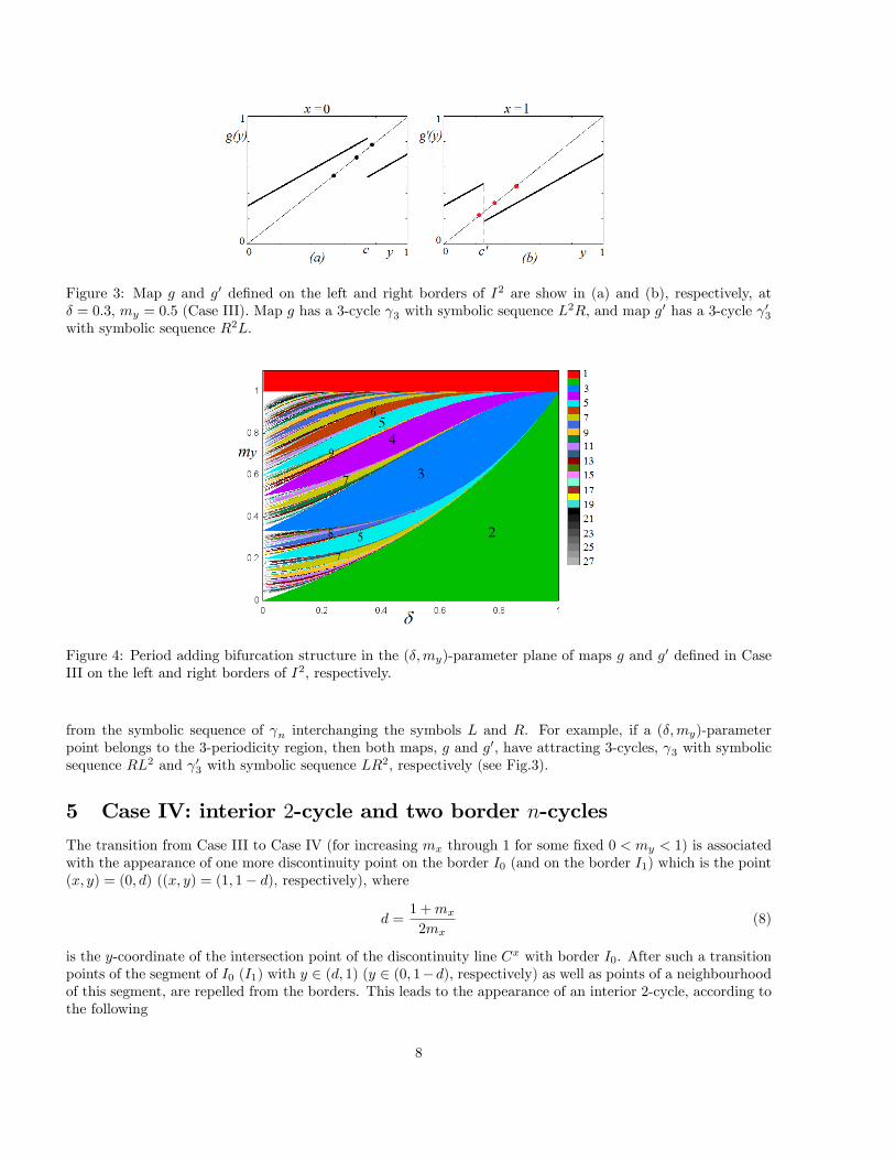
Figure 3: Map g and g0 de�ned on the left and right borders of I2 are show in (a) and (b), respectively, at� = 0:3; my = 0:5 (Case III). Map g has a 3-cycle 3 with symbolic sequence L

2R; and map g0 has a 3-cycle 03with symbolic sequence R2L.

Figure 4: Period adding bifurcation structure in the (�;my)-parameter plane of maps g and g0 de�ned in CaseIII on the left and right borders of I2, respectively.

from the symbolic sequence of n interchanging the symbols L and R. For example, if a (�;my)-parameterpoint belongs to the 3-periodicity region, then both maps, g and g0; have attracting 3-cycles, 3 with symbolicsequence RL2 and 03 with symbolic sequence LR

2; respectively (see Fig.3).

5 Case IV: interior 2-cycle and two border n-cycles

The transition from Case III to Case IV (for increasing mx through 1 for some �xed 0 < my < 1) is associatedwith the appearance of one more discontinuity point on the border I0 (and on the border I1) which is the point(x; y) = (0; d) ((x; y) = (1; 1� d); respectively), where

d =1 +mx

2mx(8)

is the y-coordinate of the intersection point of the discontinuity line Cx with border I0. After such a transitionpoints of the segment of I0 (I1) with y 2 (d; 1) (y 2 (0; 1�d); respectively) as well as points of a neighbourhoodof this segment, are repelled from the borders. This leads to the appearance of an interior 2-cycle, according tothe following

8

Property 3. For any �xed 0 < � < 1 and mx > 1, my < 1 map F has an interior attracting 2-cycle�2 = fp0; p1g; where

p0 =

�1

2� � ;1� �2� �

�2 D1; p1 =

�1� �2� � ;

1

2� �

�2 D2 (9)

To see this, note that considering map F 2 = F2 � F1; its �xed point p0 is a point of an actual 2-cycle of mapF if p0 2 D1 (in such a case p1 = F (p0) 2 D2 due to the symmetry), that holds for mx > 1, my < 1; i.e., for(mx;my) 2 RIV [RV . For mx = 1 a BCB of �2 occurs at which p0 2 Cx (and also p1 2 Cx), while for my = 1a BCB occurs at which p0 2 Cy (as well as p1 2 Cy), so that in the (mx;my)-parameter plane the boundaries ofthe periodicity region associated with an interior 2-cycle are de�ned by the straight lines my = 1 and mx = 1.

For (mx;my) 2 RIV the 2-cycle �2 = fp0; p1g (see Property 3) may coexist or not with border cycles n 2 I0and 0n 2 I1; or, in a non generic case, with Cantor set attractors q� 2 I0 and q0� 2 I1.In fact, the periodicity regions forming the period adding structure in region RIII extend to region RIV ;

however, in RIV each region has one more, vertical, boundary (see, for example, Fig.2), related to the mentionedabove new discontinuity points (x; y) = (0; d) 2 I0 and (x; y) = (1; 1 � d) 2 I1. To see which bifurcation isassociated with this boundary consider map g given in (7) and its absorbing interval J = [gR(c); gL(c)] to whichthe related cycle n belongs (the cycle

0n belongs, respectively, to the absorbing interval J

0 = [gR(c0); gL(c

0)]).For (mx;my) 2 RIV map g is de�ned not on the complete border I0; i.e., not for any y 2 [0; 1] as in Case III,but for y 2 [0; d]; and any point (x; y) = (0; y) with y > d is mapped in the interior of I2. As long as gL(c) < d;that is, if d =2 J , the period adding structure of map F is not in�uenced by the existence of point d, that is, itextends from region RIII to region RIV . If gL(c) = d that holds for

B : my =1� �mx

mx(1� �)(10)

the absorbing interval J has a contact with d (see Fig.2 where curve B is shown). If gL(c) > d; i.e., if d 2 J;new discontinuity point y = d can collide (for increasing mx) with the rightmost point of cycle n; and thisBCB de�nes the vertical borders of the periodicity regions in RIV (their analytical expressions are given inAppendix). A collision of the discontinuity point y = c can no longer occur with n from the right side (becausesuch a collision means also a collision of the critical point gL(c) with the rightmost point of n) and, thus, theperiodicity regions in RIV have no lower BCB boundary, while such a collision from the left side can still occur(for increasing my), and this BCB is associated with the upper boundary of the related periodicity region.

Figure 5: Case IV. Coexisting attracting interior 2-cycle and two border 3-cycles together with their basins.Here � = 0:3 and (mx;my) = (1:3; 0:45) in (a), (mx;my) = (1:75; 0:45) in (b), so that the (mx;my)-parameterpoint is, respectively, below and above curve B given in (10).

Clearly, the appearance of an attracting internal cycle �2 leads to a change in the basins of attraction ofthe cycles n and

0n, moreover, these basins di¤er depending on the location of the (mx;my)-parameter point

9

wrt curve B. Recall that for (mx;my) 2 RIII the basins of n and 0n are separated by the discontinuity lineCx: For (mx;my) 2 RIV with my <

1��mx

mx(1��) ; that is, if (mx;my)-point is below the curve B, the basins of nand 0n remain simply connected (see an example in Fig.5a where an interior 2-cycle coexists with two border3-cycles). On the other hand, for (mx;my) 2 RIV with my >

1��mx

mx(1��) ; that is, if (mx;my)-point is above the

curve B, the basins of n and 0n are disconnected in I

2 (an example is shown in Fig.5b). All the basins areseparated by the proper segments of the discontinuity lines Cx, Cy and their preimages. It is worth to note alsothat curve B converges to curve C as � ! 0, that is, the subregion of RIV associated with disconnected basinsdecreases and disappears as � ! 0.In the transition from Case IV to Case V crossing the curve C given in (6), for example, increasing my for

�xed mx > 1 (see e.g., Fig.2), the discontinuity curves Cx and Cy are merging and switching their position wrteach other. As a result, in the parameter region above the curve C the cycles n and

0n no longer exist (it can

be shown that in a lower neighbourhood of the curve C only the basic cycles n 2 I0 and 0n 2 I1, n � 1, withsymbolic sequences LnR and RnL, respectively, still exist), while new interior cycles may appear as we show inthe next section.

6 Cases V, VI: Interior cycles and period incrementing structures

6.1 Border collision bifurcations of an interior cycle

Let us denote an interior cycle of map F as �2n = fpig2n�1i=0 = f(xi; yi)g2n�1i=0 ; n � 1: We represent such a cycleby a symbolic sequence � = �0�1:::�2n�1 where �i 2 f1; 2; 3; 4g and

�i =

8>><>>:1 if pi 2 D1

2 if pi 2 D2

3 if pi 2 D3

4 if pi 2 D4

Property 4. Let (mx;my) 2 RV [ RV I . Any interior cycle �2n; n � 1; of map F can be represented by thesymbolic sequence 1k4l2k3l where k � 1; l � 0. The period of �2n can be written as 2n = 2(k + l).To see this consider �rst an arbitrary initial point q0 = (x0; y0) 2 D1: Applying map F1 the trajectory moves

along the straight line y = y0�1x0

x+ 1 approaching the �xed point (x; y) = (0; 1) of map F1. Two cases can bedistinguished:(1) If after a number i � 1 of iterations by F1 it holds that qi = F i1(q0) 2 D2 (this can occur if (mx;my) 2

RV and cannot occur if (mx;my) 2 RV I), then applying F2 the trajectory moves along the straight liney = yi

xi�1 (x � 1) towards the �xed point (x; y) = (1; 0) of F2: It is easy to see that the trajectory necessarilycomes back to D1 where F1 is applied again. As a result, applying only the maps F1 and F2; the trajectory isattracted to the 2-cycle �2 (see Property 3) which can be represented by the symbolic sequence 11402130: Herethe upper index 0 means that the related symbol is absent in the symbolic sequence. The parameter regionde�ned by mx > 1; my < 1; associated with �2 is denoted P0;1.(2) If after a number i � 1 of iterations by F1 it holds that qi = F i1(q0) 2 D4 (this can occur for (mx;my) 2

RV and necessarily occurs for (mx;my) 2 RV I), then applying map F4 the trajectory moves along the straightline y = 1�yi

1�xix + 1 towards the �xed point (x; y) = (1; 1) of map F4; and after a number j � 1 of iterations itnecessarily enters region D2, that is, qi+j = F j4 � F i1(p0) 2 D2. Then, after a number of iterations by F2 thetrajectory enters region D3; and applications by F3 lead the trajectory back to region D1. In such a way a cycle(of period at least 4) of map F may exist.Consider a cycle �2n = fpig2n�1i=0 of map F; n � 2, where p0 is the rightmost periodic point in D1. Then

following the same reasoning as for a generic trajectory, we can state that there are numbers k � 1 and l � 1such that pk = F k1 (p0) 2 D4 and pk+l = F l4 � F k1 (p0) 2 D2: Due to the symmetry of F wrt S; point pk+l isnecessarily symmetric wrt S to point p0, that is, it holds pk+l = (1�x0; 1�y0), and there are other k�1 pointsof �2n in D2 as well as l points in D3; each of which is symmetric to the related point pi; 1 � i � k + l � 1.Thus, the cycle �2n can be represented by the symbolic sequence 1k4l2k3l. We denote its existence region inthe (mx;my)-parameter plane as Pl;k. Two examples of �2n are presented in Fig.6.

10

Figure 6: Examples of interior cycles �2(k+l) = fpig2(k+l)�1i=0 of map F with k points in region D1; l points inD4; k points in region D2 and l points in region D3. In case (a) the related periodicity region Pl;k has fourboundaries, while in case (b) Pl;k is unbounded on two sides (see Proposition 1).

Property 5. The rightmost point p0 2 D1 of the cycle �2n = fpig2n�1i=0 ; n � 1; of map F with symbolicsequence 1k4l2k3l has the following coordinates:

p0 = (x0; y0) =

�al

1 + al+k;

al+k

1 + al+k

�; a := 1� � (11)

To see this note that for p0 2 D1; where p0 is the point of �2n in D1 with the largest x0 coordinate, it holds

pk+l = (al(akx0 � 1) + 1; al+k(y0 � 1) + 1)

then (11) follows from pk+l = (1� x0; 1� y0):

Proposition 1 Let 0 < � < 1; a = 1 � �; and (mx;my) 2 RV [ RV I . Suppose map F has a cycle �2n =fpig2n�1i=0 ; n � 2: Then it is an interior attracting cycle of period 2(k + l) with the symbolic sequence 1k4l2k3l,where 1 � l � l; k � l; and l =

�log1�� 0:5

�+ 1. In the (mx;my)-parameter plane the related periodicity region

Pl;k is con�ned by at most four boundaries associated with the border collision bifurcations of �2n:

B1l;k : my =al+k � 1

1 + al(ak � 2) =: m1y(l;k) (p0 2 Cy) (12)

B2l;k : my =al+k�1(2� a)� 11 + al�1(ak+1 � 2) =: m

2y(l;k) (p2(k+l)�1 2 Cy) (13)

B3l;k : mx =1� al+k

1 + ak(al � 2) =: m3x(l;k) (pk 2 Cx) (14)

B4l;k : mx =1� al+k�1(2� a)1 + ak�1(al+1 � 2) =: m

4x(l;k) (pk�1 2 Cx) (15)

The region Pl;k can be one-side unbounded (only the boundaries B1l;k; B2l;k and B

3l;k; or B

2l;k; B

3l;k and B

4l;k; exist)

or two-side unbounded (only the boundaries B2l;k and B3l;k exist).

Proof. Let 0 < � < 1, (mx;my) 2 RV [ RV I : Suppose that map F has a cycle �2n = fpig2n�1i=0 ; n � 1: Then�2n can be represented by the symbolic sequence 1k4l2k3l (see Property 4), where 1 � l � l; k � l (the value l isdiscussed in Proposition 2), and the rightmost point p0 2 D1 of �2n has coordinates given in (11) (see Property5).

11

Increasing my (the slope of the discontinuity line Cy given in (5) becomes larger in modulus, see Fig.7a) aBCB of �2n can occur at which p0 2 Cy. From the condition p0 2 Cy the boundary B1l;k of Pl;k is obtained (seeFig.7b). Obviously, such a BCB cannot occur if x0 � 1

2 (see Fig.6b) given that it must hold my > 0 (i.e., theslope of Cy must be negative). Thus, if x0 � 1

2 ; that is, if 1 + al(ak � 2) � 0; the boundary B1l;k of Pl;k doesnot exist and Pl;k is at least one-side unbounded. Note that in such a case it holds that m1

y(l;k) < 0:

Figure 7: Approaching boundary B1l;k of the periodicity region Pl;k by increasing my: in (a) it is shown howthe curve Cy moves, and in (b) the related boundary is indicated.

Decreasing my (the slope of Cy becomes smaller in modulus, see Fig.8a) a BCB of �2n can occur at whichp2(k+l)�1 2 Cy where

p2(k+l)�1 =

�al�1

1 + al+k;al+k�1

1 + al+k

�From the condition p2(k+l)�1 2 Cy the boundary B2l;k is obtained (see Fig.8b). It is easy to see that for theconsidered parameter values such a BCB always occurs, that is, the boundary B2l;k of Pl;k always exists.

Figure 8: Approaching boundary B2l;k of the periodicity region Pl;k by decreasing my: in (a) it is shown howthe curve Cy moves, and in (b) the related boundary is indicated.

Let now mx be decreasing (the slope of the discontinuity line Cx de�ned in (5) becomes larger in modulus,see Fig.9a). Then a BCB of �2n can occur at which pk 2 Cx where

pk =

�al+k

1 + al+k;1 + ak(al � 1)1 + al+k

�

12

The equation for B3l;k is obtained from the condition pk 2 Cx (Fig.9b). For the considered parameter valuessuch a BCB always occurs so that the boundary B3l;k of Pl;k always exists.

Figure 9: Approaching boundary B3l;k of the periodicity region Pl;k by decreasing mx: in (a) it is shown howthe curve Cx moves, and in (b) the related boundary is indicated.

Increasing mx (the slope of Cx becomes smaller in modulus, see Fig.10a) a BCB of �2n can occur at whichpk�1 2 Cx where

pk�1 =

�al+k�1

1 + al+k;1 + ak�1(al+1 � 1)

1 + al+k

�The equation for B4l;k is obtained from pk�1 2 Cx (see Fig.10b). Such a BCB cannot occur if yk�1 � 1

2 (seeFig.6b) given that it must hold mx > 0 (i.e., the slope of Cx must be negative). Thus, if yk�1 � 1

2 ; that is,if 1 + ak�1(al+1 � 2) � 0; it holds that the boundary B4l;k of Pl;k does not exist and Pl;k is at least one-sideunbounded. Note that in such a case m4

x(l;k) < 0 (in (15) the inequality 1 � al+k�1(2 � a) > 0 follows from

xl+k�1 <12 ).

Figure 10: Approaching boundary B4l;k of the periodicity region Pl;k by increasing mx: in (a) it is shown howthe curve Cx moves, and in (b) the related boundary is indicated.

To summarize, if all the BCB values given in (12)-(15) are positive, it holds that m1y(l;k) > m2

y(l;k) andm4x(l;k) > m3

x(l;k), that is, B1l;k; B

2l;k; B

3l;k and B

4l;k are, respectively, upper, lower, left and right boundaries of

Pl:k: If for some values of k; l it holds that m1y(l;k) < 0 (i.e., 1+ a

l(ak � 2) > 0) then such a region is unboundedfrom above, while if m4

x(l;k) < 0 (i.e., 1 + ak�1(al+1 � 2) < 0) holds then the related region is unbounded fromthe right.

13

Figure 11: BCB boundaries of the periodicity regions Pl;k; l = 1; 2; k � l, in the (arctan(mx); arctan(my))-parameter plane for � = 0:3:

6.2 Properties of the period incrementing structures

Fig.11a shows an example of the BCB boundaries con�ning the periodicity regions Pl;k in the (arctan(mx);arctan(my))-parameter plane for � = 0:3 (some boundaries are shown in color associated with the collidingcycle). As we show below (see Proposition 2), for such a value of � it holds that l � l = 2; that is, thereare two sets of periodicity regions, fP1;kg1k=1 and fP2;kg

1k=2 ; which are related to the cycles with symbolic

sequences 1k412k31 and 1k422k32: In Fig.11b the BCB boundaries of the periodicity regions are superposedon the 2D bifurcation diagram obtained numerically. One can see that the regions P1;k and P1;k+1; k � 1,are partially overlapping and for k ! 1 they accumulate to mx = 1+: So, the set of regions fP1;kg1k=1 forma period incrementing bifurcation structure with incrementing step 2. The same holds for regions fP2;kg1k=2.Note that regions P1;1 and P2;2 are two side unbounded, P1;2 is unbounded from the right and P2;k; k � 3; areunbounded from above. Note also that the periodicity regions of di¤erent incrementing structures, that is, forl = 1 and l = 2, are also partially overlapping, so that more than 2 di¤erent cycles may coexist. An example of4 coexisting cycles11 is shown in Fig.12b, and the related parameter point is indicated in Fig.12a.

Proposition 2 For a �xed 0 < � < 1 the number of the period incrementing bifurcation structures in the(mx;my)-parameter plane of map F is given by

l =�log1�� 0:5

�+ 1 (16)

that is, map F can have cycles with symbolic sequences 1k4l2k3l for any 1 � l � l and k � l: Here b�c denotesthe integer part of the number.

Proof. Suppose that 0 < � < 1 is �xed and in the (mx;my)-parameter plane of map F there is more thanone period incrementing structure. Consider a set of periodicity regions fPl;kg1k=l for some �xed l � 2: For theboundaries of these regions, de�ned in (12)-(15), we have

limk!1

m3x(l;k) = 1; lim

k!1m4x(l;k) = 1

limk!1

m1y(l;k) =

1

2(1� �)l � 1 =: my;l (17)

11As it follows from Proposition 2 the number of incrementing structures increases as � ! 0: Then more than 2 incrementingstructures can overlap leading to more than 4 coexisting cycles.

14

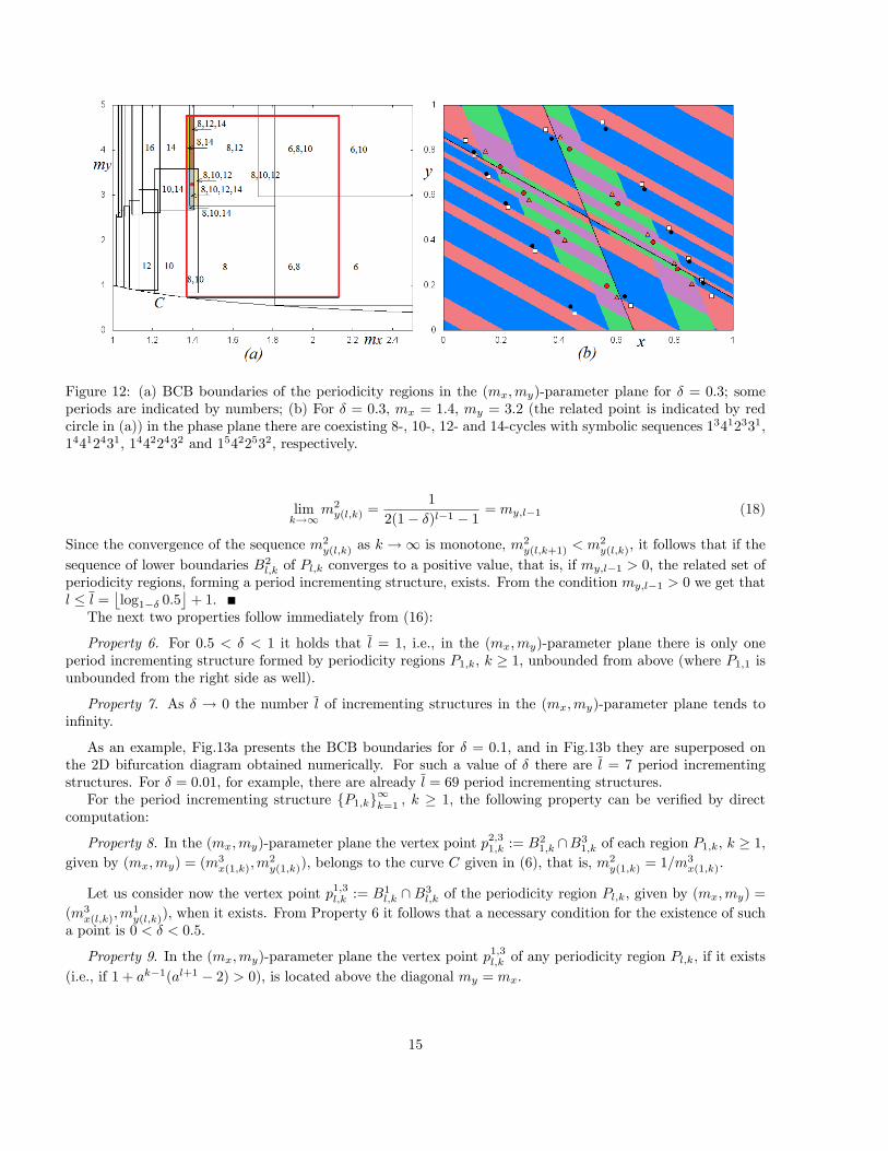
Figure 12: (a) BCB boundaries of the periodicity regions in the (mx;my)-parameter plane for � = 0:3; someperiods are indicated by numbers; (b) For � = 0:3; mx = 1:4; my = 3:2 (the related point is indicated by redcircle in (a)) in the phase plane there are coexisting 8-, 10-, 12- and 14-cycles with symbolic sequences 13412331;14412431; 14422432 and 15422532, respectively.

limk!1

m2y(l;k) =

1

2(1� �)l�1 � 1 = my;l�1 (18)

Since the convergence of the sequence m2y(l;k) as k !1 is monotone, m2

y(l;k+1) < m2y(l;k), it follows that if the

sequence of lower boundaries B2l;k of Pl;k converges to a positive value, that is, if my;l�1 > 0; the related set ofperiodicity regions, forming a period incrementing structure, exists. From the condition my;l�1 > 0 we get thatl � l =

�log1�� 0:5

�+ 1.

The next two properties follow immediately from (16):

Property 6. For 0:5 < � < 1 it holds that l = 1; i.e., in the (mx;my)-parameter plane there is only oneperiod incrementing structure formed by periodicity regions P1;k, k � 1; unbounded from above (where P1;1 isunbounded from the right side as well).

Property 7. As � ! 0 the number l of incrementing structures in the (mx;my)-parameter plane tends toin�nity.

As an example, Fig.13a presents the BCB boundaries for � = 0:1; and in Fig.13b they are superposed onthe 2D bifurcation diagram obtained numerically. For such a value of � there are l = 7 period incrementingstructures. For � = 0:01; for example, there are already l = 69 period incrementing structures.For the period incrementing structure fP1;kg1k=1 ; k � 1, the following property can be veri�ed by direct

computation:

Property 8. In the (mx;my)-parameter plane the vertex point p2;31;k := B21;k \B31;k of each region P1;k; k � 1;

given by (mx;my) = (m3x(1;k);m

2y(1;k)); belongs to the curve C given in (6), that is, m2

y(1;k) = 1=m3x(1;k).

Let us consider now the vertex point p1;3l;k := B1l;k \ B3l;k of the periodicity region Pl;k; given by (mx;my) =

(m3x(l;k);m

1y(l;k)); when it exists. From Property 6 it follows that a necessary condition for the existence of such

a point is 0 < � < 0:5:

Property 9. In the (mx;my)-parameter plane the vertex point p1;3l;k of any periodicity region Pl;k; if it exists

(i.e., if 1 + ak�1(al+1 � 2) > 0), is located above the diagonal my = mx:

15

Figure 13: BCB boundaries of the periodicity regions Pl:k; 1 � l � 7; k � l; in the (arctan(mx); arctan(my))-parameter plane for � = 0:1:

A simple corollary of this property is that regions P1;k; k � 1, extend from the parameter region RV to theparameter region RV I : Moreover, the following property holds:

Property 10. In the parameter region RV there is only the period incrementing structure fP1;kg1k=1 (extend-ing to RV I) which is overlapped by region P0;1 related to 2-cycle �2 (see Property 3).

To see this, note that for 0 < � < 0:5 it holds that my;1 =1

1�2� > 1; my;2 = 1 (see (17), (18)) and for anyk � 2 we have that m2

y(2;k+1) < m2y(2;k), that is, the period incrementing structure fP2;kg

1k=2 is located in RV I :

The above property means that for (mx;my) 2 RV map F has an interior 2-cycle �2 which may coexist ornot with one cycle having symbolic sequence 1k412k31; k � 1, or with two such cycles, with symbolic sequence1k412k31 and 1k+1412k+131: For example, in Fig.14a an interior 2-cycle coexists with 8-cycle 13412331, and inFig.14b it coexists with 6-cycle 12412231 and 8-cycle 13412331.

Figure 14: Coexisting interior 2- and 8-cycles in (a) and 2-, 6- and 8-cycles in (b), and their basins. Here� = 0:3; my = 0:8 and mx = 1:5 in (a) and mx = 2 in (b).

16

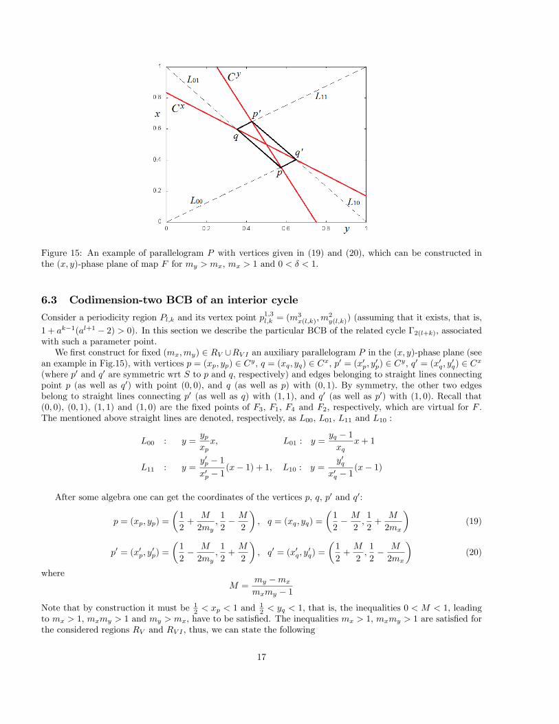
Figure 15: An example of parallelogram P with vertices given in (19) and (20), which can be constructed inthe (x; y)-phase plane of map F for my > mx; mx > 1 and 0 < � < 1.

6.3 Codimension-two BCB of an interior cycle

Consider a periodicity region Pl;k and its vertex point p1;3l;k = (m

3x(l;k);m

2y(l;k)) (assuming that it exists, that is,

1 + ak�1(al+1 � 2) > 0). In this section we describe the particular BCB of the related cycle �2(l+k); associatedwith such a parameter point.We �rst construct for �xed (mx;my) 2 RV [RV I an auxiliary parallelogram P in the (x; y)-phase plane (see

an example in Fig.15), with vertices p = (xp; yp) 2 Cy, q = (xq; yq) 2 Cx; p0 = (x0p; y0p) 2 Cy, q0 = (x0q; y0q) 2 Cx(where p0 and q0 are symmetric wrt S to p and q, respectively) and edges belonging to straight lines connectingpoint p (as well as q0) with point (0; 0); and q (as well as p) with (0; 1): By symmetry, the other two edgesbelong to straight lines connecting p0 (as well as q) with (1; 1); and q0 (as well as p0) with (1; 0): Recall that(0; 0); (0; 1); (1; 1) and (1; 0) are the �xed points of F3; F1; F4 and F2; respectively, which are virtual for F .The mentioned above straight lines are denoted, respectively, as L00; L01; L11 and L10 :

L00 : y =ypxpx; L01 : y =

yq � 1xq

x+ 1

L11 : y =y0p � 1x0p � 1

(x� 1) + 1; L10 : y =y0q

x0q � 1(x� 1)

After some algebra one can get the coordinates of the vertices p; q; p0 and q0:

p = (xp; yp) =

�1

2+

M

2my;1

2� M

2

�; q = (xq; yq) =

�1

2� M

2;1

2+

M

2mx

�(19)

p0 = (x0p; y0p) =

�1

2� M

2my;1

2+M

2

�; q0 = (x0q; y

0q) =

�1

2+M

2;1

2� M

2mx

�(20)

whereM =

my �mx

mxmy � 1Note that by construction it must be 1

2 < xp < 1 and 12 < yq < 1, that is, the inequalities 0 < M < 1; leading

to mx > 1; mxmy > 1 and my > mx; have to be satis�ed. The inequalities mx > 1; mxmy > 1 are satis�ed forthe considered regions RV and RV I ; thus, we can state the following

17

Figure 16: Period incrementing structure fP3;kg1k=3 for � = 0:1 (a) and � = 0:05 (b). The curves Vk de�ned in(21), to which the vertex points p1;3l;k belong, are shown for 1 � k � 100. The region P3;5 is highlighted.

Property 11. In the (x; y)-phase plane of map F a parallelogram P with vertices p; q; p0 and q0, given in(19) and (20), can be constructed if my > mx; mx > 1; independently on �.

The following property can be veri�ed by straightforward calculations:

Property 12. The vertex point p1;3l;k of region Pl;k is a codimension-2 BCB point at which four points of thecycle �2(l+k) collide with the borders: p0 = p 2 Cy; pk = q 2 Cx, pk+l = p0 2 Cy and p2k+l = q0 2 Cx; wherep; q; p0 and q0 are given in (19) and (20).

Recall that at the parameter point p1;3l;k the inequality m1y(l;k) > m3

x(l;k) holds, thus, from Property 11 itfollows that the parallelogram P can be constructed.Note that from p0 = p it follows that points p1;3l;k for di¤erent k belong to the curves

Vk : my =akmx

mx(ak � 1) + 1(21)

which for �xed k and � ! 0 (i.e., a! 1�) tend to the diagonal my = mx; while for �xed � and k !1 tend tothe vertical line mx = 1. In Fig.16 the curves Vk are shown for 1 � k � 100 and � = 0:1 in Fig.16a, � = 0:05 inFig.16b.

It is interesting to note that as mx ! 1+; it holds that p !�my+12my

; 0�; q ! (0; 1) ; p0 !

�my�12my

; 1�and

q0 ! (1; 0) (see (19) and (20)). We can formulate the following

Property 13. Let my > 1 and 0 < � < 1 be �xed and mx ! 1+: Then for interior cycles �2(l+k) it holds thatk !1 and points pk�1 and pk tend to (0; 1); while the symmetric points p0k�1 = p2k+l�1 and p0k = p2k+l tendto (1; 0). Crossing the boundary mx = 1 (so that the (mx;my) parameter point enters region RI) leads to theattracting �xed points (x; y) = (0; 1) and (x; y) = (1; 0).

Proposition 3 Let 0 < � < 1, my > mx and mx > 1: Then in the generic case any initial point (x0; y0) isattracted to a cycle �2n; n � 2, of map F , and points of this cycle are external to the parallelogram P withvertices p; q; p0 and q0, given in (19) and (20).

Proof. Generic case here means that the (mx;my)-parameter point does not belong to a BCB boundary of someperiodicity region. To prove this statement let us consider a non-generic case related to the parameter pointp1;3l;k at which p0 2 Cy and pk 2 Cx and p0 = p; pk = q (see Property 9). Then increasing mx and decreasing my

(so that the parameter point enters the region Pl;k) the points of the cycle �2(l+k) remain unchanged becausetheir coordinates do not depend on mx; my, while the vertices of parallelogram P move towards point S : it is

18

easy to check that for increasing mx and decreasing my the value yp increases, thus, the value xp decreases, sothat the vertex p becomes closer to S, and the same conclusion holds also for the other vertices of P . Thus, thepoints of the cycle, when it exists (i.e., for (mx;my) 2 Pl;k), cannot be located inside parallelogram P (recallthat parallelogram P shrinks to point S for my = mx, and does not exist for my < mx).

7 Discrete versus continuous time model: a comparison of dynamics

As we already mentioned map F given in (4) describes the dynamics of a discrete-time version of the continuous-time fashion cycle model � given in (1). In the present section we show that the dynamics of map F as � ! 0converge to those of the original continuous-time model. Recall that the discrete-time and continuous-timeversions are related via 1 � � = e��4, and � ! 0 as 4 ! 0, where 4 is the time-delay in the discrete timeformulation.Similar to the partitioning of the (mx;my)-parameter plane of the discrete-time model, the (m;m�)-parameter

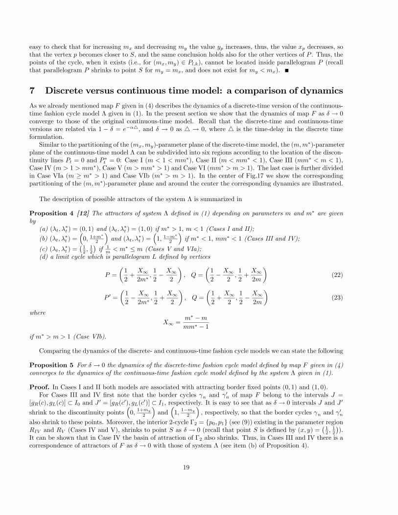
plane of the continuous-time model � can be subdivided into six regions according to the location of the discon-tinuity lines Pt = 0 and P �t = 0: Case I (m < 1 < mm�), Case II (m < mm� < 1), Case III (mm� < m < 1),Case IV (m > 1 > mm�), Case V (m > mm� > 1) and Case VI (mm� > m > 1). The last case is further dividedin Case VIa (m � m� > 1) and Case VIb (m� > m > 1). In the center of Fig.17 we show the correspondingpartitioning of the (m;m�)-parameter plane and around the center the corresponding dynamics are illustrated.

The description of possible attractors of the system � is summarized in

Proposition 4 [12] The attractors of system � de�ned in (1) depending on parameters m and m� are givenby(a) (�t; �

�t ) = (0; 1) and (�t; �

�t ) = (1; 0) if m

� > 1; m < 1 (Cases I and II);

(b) (�t; ��t ) =

�0; 1+m

�

2

�and (�t; �

�t ) =

�1; 1�m

�

2

�if m� < 1; mm� < 1 (Cases III and IV);

(c) (�t; ��t ) =

�12 ;

12

�if 1

m < m� � m (Cases V and VIa);(d) a limit cycle which is parallelogram L de�ned by vertices

P =

�1

2+X12m� ;

1

2� X1

2

�; Q =

�1

2� X1

2;1

2+X12m

�(22)

P 0 =

�1

2� X12m� ;

1

2+X12

�; Q =

�1

2+X12;1

2� X12m

�(23)

where

X1 =m� �mmm� � 1

if m� > m > 1 (Case VIb).

Comparing the dynamics of the discrete- and continuous-time fashion cycle models we can state the following

Proposition 5 For � ! 0 the dynamics of the discrete-time fashion cycle model de�ned by map F given in (4)converges to the dynamics of the continuous-time fashion cycle model de�ned by the system � given in (1).

Proof. In Cases I and II both models are associated with attracting border �xed points (0; 1) and (1; 0).For Cases III and IV �rst note that the border cycles n and

0n of map F belong to the intervals J =

[gR(c); gL(c)] � I0 and J 0 = [gR(c0); gL(c0)] � I1, respectively. It is easy to see that as � ! 0 intervals J and J 0

shrink to the discontinuity points�0;

1+my

2

�and

�1;

1�my

2

�; respectively, so that the border cycles n and

0n

also shrink to these points. Moreover, the interior 2-cycle �2 = fp0; p1g (see (9)) existing in the parameter regionRIV and RV (Cases IV and V), shrinks to point S as � ! 0 (recall that point S is de�ned by (x; y) =

�12 ;

12

�).

It can be shown that in Case IV the basin of attraction of �2 also shrinks. Thus, in Cases III and IV there is acorrespondence of attractors of F as � ! 0 with those of system � (see item (b) of Proposition 4).

19

Figure 17: In the center: Partitioning of the (m;m�)-parameter plane into the regions associated with di¤erentcases of continuous time fashin cycle model �. Around the center: The (�t; �

�t )-phase plane where examples of

the discontinuity lines and attractors, corresponding to these regions, are shown.

In Case VI for my � mx; as well as in Case V, i.e., for the (mx;my)-parameter point satisfying 1mx

� my �mx, the trajectories of map F as � ! 0 tend to point S, as illustrated by the 1D bifurcation diagrams � versusx for my = 2 and mx = 3 in Fig.18a, and my = mx = 2 in Fig.18b. Recall that map F can have coexistingcycles, and some of them are shown in Fig.18 by di¤erent colors. As one can see, for decreasing � points of eachcycle, as long as this cycle exists, tend to S, however, such a cycle may disappear due to a BCB.In fact, let 0 < � < 1 be �xed. Consider a parameter point (mx;my) satisfying 1

mx� my � mx. Such a

point necessarily belongs to one or several (overlapping) periodicity regions. Let (mx;my) 2 Pl;k; then map Fhas the cycle �2(l+k) with point p0 2 D1 de�ned in (11). From (11) it follows that decreasing � the point p0 (aswell as any other point of �2(l+k)) tends to S: In the meantime, decreasing � the value m1

y(l;k) (related to theBCB boundary B1l;k) decreases and the value m

3x(l;k) (related to B

3l;k) increases, that can be veri�ed using (21).

It is illustrated in Fig.16, where the region P3;5 is highlighted for � = 0:1 in Fig.16a and � = 0:05 in Fig.16b.Thus, decreasing � cycle �2(l+k) either shrinks to S; or disappears due to a BCB colliding either with Cy (ifboundary B1l;k is crossed) or with C

x (if B3l;k is crossed). Given that for each �xed my � mx and decreasing �the period of cycles of map F may increase but it remains �nite (i.e., l and k in (11) do not tend to in�nity), itholds that in the considered case the limit sets of the trajectories of F shrink to S, i.e., there is a correspondence

20

Figure 18: 1D bifurcation diagram � versus x of map F for 0 < � < 0:1, my = 2 and (a) mx = 3; (b) mx = 2;(c) mx = 1:5.

with item (c) of Proposition 4.In Case VI for my > mx the trajectories of map F as � ! 0 tend to cycles whose period tends to in�nity

and whose location tends to the parallelogram P with vertices de�ned in (19), (20) (note that these verticescorrespond to those de�ned in (22), (23)). This case is illustrated in Fig.18c, where the 1D bifurcation diagram� versus x is shown for my = 2 and mx = 1:5. Here the points xq and x0q which are x-coordinates of the verticesq and q0 of P , are also indicated. Note that for mx ! 1+ it holds that xq ! 0 and x0q ! 1.

Figure 19: (a) In Case VI for my > mx and � ! 0 limit sets of trajectories of map F tend to parallelogram P ;(b) the related parallelogram and convergence to it in the continuous-time fashion cycle model.

In fact, similarly to the previous case, for �xed (mx;my) 2 Pl;k (with my > mx) and decreasing � the pointsof the related cycle �2(l+k) tend to S; however, �2(l+k) necessarily disappears due to a BCB colliding eitherwith Cy when the boundary B1l;k is crossed, or with C

x when B3l;k is crossed (recall that as � ! 0 the point p1;3l;ktends to the diagonal my = mx, with decreasing m1

y(l;k) and increasing m3x(l;k)). Each new cycle which appears

for decreasing � has a higher period, moreover, according to Proposition 3, any cycle of map F remains externalto the parallelogram P (recall that its vertices do not depend on �). Thus, parallelogram P is a limit set forthe trajectories of map F as � ! 0; which corresponds to item (d) of Proposition 4 (see Fig.19 where one cancompare the parallelograms and trajectories of discrete- and continuous-time models in Case VIb).

21

8 Concluding remarks

We considered a 2D piecewise linear discontinuous map F depending on three parameters, which is a discrete-time version of the continuous-time fashion cycle model introduced in [12]. The map is chartarized by attractingcycles of di¤erent periods, with possible coexistence. Our objective was twofold: to describe the bifurcationstructure of the parameter space of map F and to compare the obtained results with those associated withthe continuous-time model. In fact, the bifurcation structure of map F is quite interesting: it is formed bythe periodicity regions of attracting cycles organized in the period adding and period incrementing bifurcationstructures. Recall that these structures are known to be characteristic for 1D piecewise monotone maps with onediscontinuity point. In map F the period adding structure is standard being observed when map F is reducedto a 1D piecewise linear map. As for the period incrementing structure, it is related to the 2D dynamics andassociated with the following peculiarities: if the coe¢ cient of the contraction of the linear maps de�ning Fis larger than 1=2 then several partially overlapping period incrementing structures are observed, moreover,their number goes to in�nity if the contraction coe¢ cient tends to 1 (that corresponds also to the time-delayin the discrete time formulation of the model tending to zero). This leads, in particular, to more than twocoexisting attracting cycles whose basin boundaries are formed by proper segments of discontinuity lines andtheir preimages. The rather simple analytical representation of map F allowed us to get the boundaries of allthe periodicity regions in explicit form. We showed also that the dynamics of map F converges to the dynamicsof its continuous-time counterpart if the time-delay in the discrete time formulation of the model tends to zero.The question arises to which extent the considered fashion cycle model can be generalized. One possible

direction is to break the symmetry of map F . Recall that in the present formulation the map is symmetric wrtthe point (x; y) = (1=2; 1=2) which is the intersection point of two discontinuity lines. We expect that if this pointis no longer in the center of the unit square, the overall bifurcation structure will be only quantitatively modi�ed.However, a de�nite answer to this question requires further research. It is also interesting to investigate theconditions for the existence of multiple overlapping period incrementing structures in a generic 2D piecewiselinear map with one or two discontinuity lines.

ACKNOWLEDGMENTSAll the authors are grateful to the organizers and participants of Nonlinear Economic Dynamics Conference

(Pisa, Sept. 7-9, 2017) for useful discussions which helped to improve the present work. The work of L. Gardinihas been done within the activities of the GNFM (National Group of Mathematical Physics, INDAM ItalianResearch Group). I. Sushko thanks the University of Urbino for the hospitality experienced during her staythere as a Visiting Professor. K. Matsuyama is also grateful to the University of Urbino for the hospitalityduring his visit.

APPENDIXThe period adding bifurcation structure, also known as Arnold tongues or mode-locking tongues, is character-

istic for a certain class of circle maps, for discontinuous maps de�ned by two increasing functions, for nonlinearmaps undergoing Neimark-Sacker bifurcation, etc. (see, e.g. [9], [8], [4], [5]). The periodicity regions formingthis structure in the parameter space of map F given in (4) are associated with attracting n-cycles, n � 2; ofthe 1D piecewise linear discontinuous map g given in (7) de�ned on the left border of I2 (as well as with thesymmetric n-cycles of map g0 de�ned on the right border of I2). Recall that for 0 < � < 1 and my < 1; mx < 1(Case III) the left and right borders of I2 are invariant, and map F on these borders is reduced on the 1D mapsg and g0, respectively. Given that dynamics of these maps are symmetric to each other wrt points S, below weconsider the dynamics of map g only.To describe the period adding structure we �rst need to introduce the symbolic representation of a cycle.

The two partitions, 0 < y < c and c < y < 1 where c = (my + 1)=2; in which two linear branches of map g(with slopes a = 1� � < 1) are de�ned, are associated with symbols L and R: Using these symbols any genericn-cycle fyign�10 of map g can be represented by a symbolic sequence � = �0�1:::�n�1; �i 2 fL;Rg ; where�i = L if yi 2 L and �i = R if yi 2 R. The rotation number of the n-cycle can be de�ned as m=n, where n isthe number of points of the cycle (i.e., its period) and m is the number of points in the right partition. Theperiodicity regions forming the period adding structure are related to cycles with di¤erent rotation numbers.

22

These regions are ordered in the parameter space according to the Farey summation rule applied to the rotationnumbers of the related cycles, namely, between the regions corresponding to the cycles with rotation numbersm1=n1 and m2=n2 (which are Farey neighbors) there is a region related to the cycle with rotation number(m1 +m2)=(n1 + n2):A more generic de�nition of the rotation number is given as

�(y) = limn!1

1

n

nXk=0

�r(gk(y))

where �r is the characteristic function of the right partition:

�r(y) =

�0 if 0 < y < c1 if c < y < 1

For map g the rotation number is the same for any point y, �(y) := �. If � is a rational number, the abovede�nition coincides with the one given for a cycle, while if � is an irrational number then map g has a Cantorset attractor (represented by the closure of quasiperiodic trajectories). Such an attractor is not persistent underparameter perturbations.To get the boundaries of the periodicity regions analytically, all the cycles associated with the period adding

structure are �rst grouped into certain families, called complexity levels (see [9], [1], [5]). For the sake ofsimplicity we denote a cycle by its symbolic sequence. The complexity level one includes two families of basiccycles:

C1;1 = fLRn1g1n1=1 ; C2;1 = fRLn1g1n1=1 (24)

Recall that any n-cycle of map g is always attracting, with multiplier � = an < 1. Thus, its periodicity regioncan be con�ned only by the boundaries related to the BCBs. In fact, there are two boundaries: if the parameterpoint crosses one boundary then a periodic point, which is nearest from the left to the discontinuity pointy = c; collides with it, and crossing the other boundary a point of the cycle, which is nearest from the right toy = c; collides with this discontinuity point. In order to obtain analytical expressions of these boundaries it isconvenient to shift the discontinuity point of map g to the origin, introducing the new variable x := y � c: Insuch a way we obtain a topologically conjugate map

eg : x! eg(x) = � egL(x) = ax+ �(1� c); �c � x < 0egR(x) = ax� �c; 0 < x � 1� c (25)

Using the BCB conditions mentioned above and coordinates of the corresponding periodic points, one can obtainthe boundaries of the periodicity region PLRn1 related to the basic cycle LRn1 ; n1 � 1 :

�LLRn1 =

�(�;my) : 0 < � < 1; my =

2(an1 � 1)1� an1+1 + 1

��RLRn1 =

�(�;my) : 0 < � < 1; my =

2�an1�1

1� an1+1 � 1�

Similarly, the boundaries of the periodicity region PRLn1 related to the basic cycle RLn1 can be obtained:

�RRLn1 =

�(�;my) : 0 < � < 1; my = �

2(an1 � 1)1� an1+1 � 1

��LRLn1 =

�(�;my) : 0 < � < 1; my = �

2�an1�1

1� an1+1 + 1�

For example, for n1 = 1; i.e., for the basic 2-cycle RL (which is the unique basic cycle belonging to both familiesC1;1 and C2;1) the related region PRL is bounded by the curves

�LR =

�(�;my) : 0 < � < 1; my = �

�

2� �

�

23

�RL =

�(�;my) : 0 < � < 1; my =

�

2� �

�Note that in the (�;my)-parameter plane the curves �

LLRn1 and �

RRLn1 ; as well as �

RLRn1 and �

LRLn1 ; are symmetric

wrt the axis my = 0.Recall that the feasible parameter range for the considered fashion cycle model is my > 0; thus, map g has

only basic cycles associated with the family C2;1; i.e., with cycles RLn1 : In the meantime for the symmetricmap g0 the same periodicity regions correspond to the basic cycles related to the family C1;1, i.e., to cyclesLRn1 : In Fig.20 the boundaries of regionsPRLn1 and PLRn1 are shown in black for 1 � n1 � 50 in the (�; c)-and (�; c0)-parameter planes, respectively, where c = (1 + my)=2 is the discontinuity point of map g andc0 = 1� c = (1�my)=2 is the discontinuity point of map g0:In the (mx;my)-parameter plane the boundaries �

LRLn1 for n1 � 2 and �RRLn1 for n1 � 1 (which are

represented by the horizontal straight lines) extend from region RIII to region RIV (see, e.g., Fig.2) up to thecurve B de�ned in (10). Above this curve each region PRLn1 has no lower boundary while new vertical boundaryappears de�ned by a collision of the rightmost point of cycle RLn1 with the discontinuity point d given in (8):

RLn1 =

�(mx;my) : mx =

1� an1+11� an1(2� a) ; 1 +

1�mx

amx< my <

1

mx

�In the gaps between the periodicity regions PLRn1 and PLRn1+1 ; as well as PRLn1 and PRLn1+1 ; related to

the cycles of the �rst complexity level (i.e., basic cycles), the periodicity regions associated with the families ofhigher complexity levels are located. In order to get the boundaries of these regions we �rst construct for eachgap a corresponding �rst return map in a proper neighbourhood of the discontinuity point. This map appearsto be of the same class of maps as the original one. Thus, for each �rst return map we can repeat the samereasoning as for the original map and get the boundaries of the periodicity regions related to the basic cycles.For the original map these cycles are associated with 22 families of the complexity level two:

C1;2 = fLRn1 (RLRn1)n2g1n1;n2=1

; C2;2 = fRLRn1 (LRn1)n2g1n1;n2=1

C3;2 = fRLn1 (LRLn1)n2g1n1;n2=1

; C4;2 = fLRLn1 (RLn1)n2g1n1;n2=1

and the boundaries of the corresponding periodicity regions are given as

�LC1;2 =

�(�;my) : 0 < � < 1; my =

2�an1(1� a(n1+2)(n2+1))(1� an1+2)(1� an1+1+n2(n1+2)) � 1

�

�RC1;2 =

�(�;my) : 0 < � < 1; my = �

2�an1(an2(2+n1)�1(an1+2 � �)� 1)(1� an1+2)(1� an1+1+n2(n1+2)) � 1

��LC2;2 =

�(�;my) : 0 < � < 1; my =

2�an1(1� a(n1+1)(1+n2))(1� an1+1)(1� an1+2+n2(n1+1)) � 1

��RC2;2 =

�(�;my) : 0 < � < 1; my =

2an1�(1� an2(1+n1)(an1+2 + �))(1� an1+1)(1� an1+2+n2(n1+1)) � 1

�The other four boundaries are symmetric wrt my = 0, namely, �

LC3;2 is symmetric to �

RC1;2 ; �

RC3;2 to �

LC1;2 ; �

LC4;3

to �RC2;2 and, �nally, �RC4;3 to �

LC2;2 . In Fig.20 these boundaries are shown in red for 1 � n1 � 50; 1 � n2 � 10;

in the (�; c)-parameter plane for map g and in the (�; c0)-parameter plane for map g0.Reasoning in a similar way regarding the gaps between the regions of the complexity level two one can get 23

families of the complexity level three and the boundaries of the corresponding periodicity regions. This processcan be continued ad in�nitum. For more details see [1], [5] and references therein.

24

Figure 20: The period adding structure of map g given in (7) in the (�; c)-parameter plane, and of map g0

(symmetric to g) in the (�; c0)-parameter plane, where c = (1 + my)=2 and c0 = 1 � c = (1 � my)=2 are thediscontinuity points of g and g0, respectively. Here the boundaries of the periodicity regions associated withcycles of complexity level one and two are shown in black and red, respectively.

References

[1] Avrutin V., Schanz M. & Gardini L. (2010). Calculation of bifurcation curves by map replacement. Int. J.Bif. Chaos, 20, 3105-3135.

[2] Avrutin V., Sushko I. A gallery of bifurcation scenarios in piecewise smooth 1D maps. In: Global analysisof dynamic models for economics, �nance and social sciences (G.-I. Bischi, C. Chiarella and I. Sushko Eds.),Springer, 2013.

[3] M. di Bernardo, C.J. Budd, A.R. Champneys, and P. Kowalczyk, Piecewise-smooth Dynamical Systems:Theory and Applications, Applied Mathematical Sciences 163, Springer, 2008.

[4] Boyland P. L. (1986). Bifurcations of circle maps: Arnold tongues, bistability and rotation intervals. Comm.Math. Phys., 106(3), 353-381.

[5] Gardini L., V. Avrutin, I. Sushko. (2014). Codimension-2 border collision bifurcations in one-dimensionaldiscontinuous piecewise smooth maps. Int. J. Bif. Chaos, 24 (2) 1450024 (30 pages).

[6] A.J. Homburg, Global aspects of homoclinic bifurcations of vector �elds, Springer-Verlag, Berlin, 1996.

[7] S. Ito, S. Tanaka, and H. Nakada, On unimodal transformations and chaos II, Tokyo J. Math. 2 (1979),pp. 241�259.

[8] Keener J.P. (1980). Chaotic behavior in piecewise continuous di¤erence equations. Trans. Am. Math. Soc.,261, 589�604.

[9] Leonov N.N. (1959). Map of the line onto itself. Radio�sika, 3, 942�956.

[10] D.V. Lyubimov, A.S. Pikovsky, and M.A. Zaks, Universal scenarios of transitions to chaos via homoclinicbifurcations, Math. Phys. Rev. 8 (1989). Harwood Academic, London.

[11] Y.L. Maistrenko, V.L. Maistrenko, and L.O. Chua, Cycles of chaotic intervals in a time-delayed Chua�scircuit, Int. J. Bifur. Chaos 3 (1993), pp. 1557�1572.

25

[12] K. Matsuyama. Custom versus Fashion: Path-dependence and Limit Cycles in a Random Matching Game.Discussion paper N 1030, 1992, Dept of Economics, Northwestern University.

[13] C. Mira. Embedding of a Dim1 Piecewise Continuous and Linear Leonov Map into a Dim2 Invertible Map.In: Global analysis of dynamic models for economics, �nance and social sciences (G.-I. Bischi, C. Chiarellaand I. Sushko Eds.), Springer, 2013.

[14] Nusse H.E , Yorke J.A. (1992). Border-collision bifurcations including period two to period three for piece-wise smooth systems. Physica D, 57, 39�57.

[15] Nusse H.E., Yorke J.A. (1995). Border-collision bifurcations for piecewise smooth one-dimensional maps.Int. J. Bif. Chaos, 5, 189�207.

[16] Panchuk A., Sushko I., Schenke B., Avrutin V. (2013). Bifurcation Structure in Bimodal Piecewise LinearMap. Int. J. Bif. Chaos, 23(12) 1330040 (24 pages).

[17] Simpson, D. J. W. & Meiss, J. D. (2008) Neimark-Sacker bifurcations in planar, piecewise-smooth, contin-uous maps, SIAM J. Appl. Dyn. Syst. 7, 795�824.

[18] I. Sushko, V. Avrutin, and L. Gardini, Bifurcation structure in the skew tent map and its application as aborder collision normal form, J. Di¤er. Equ. Appl. (2015). doi:10.1080/10236198.2015.1113273

[19] I. Sushko, L. Gardini. Center Bifurcation for Two-Dimensional Border-Collision Normal Form, Int. J.Bifurcation and Chaos, Vol. 18, Issue 4 (2008), 1029-1050.

[20] Sushko I., L. Gardini, V. Avrutin. (2016). Nonsmooth One-dimensional Maps: Some Basic Concepts andDe�nitions. Journal of Di¤erence Equations and Applications DOI: 10.1080/10236198.2016.1248426.

[21] F. Tramontana, I. Sushko, V. Avrutin. (2015). Period adding structure in a 2D discontinuous model ofeconomic growth. Applied Mathematics and Computation, 253, 262273.

[22] Zh.T. Zhusubaliyev and E. Mosekilde, Bifurcations and Chaos in Piecewise-smooth Dynamical Systems,Nonlinear Science A Vol. 44, World Scienti�c, 2003.

[23] Z. T. Zhusubaliyev, E. Mosekilde, S. Maity, S. Mohanan, and S. Banerjee, Border collision route to quasi-periodicity: Numerical investigation and experimental con�rmation, Chaos 16, 1054 (2006).

26