2D convolution model using (in)variant kernels for fast ...

HAL Id: hal-01083451https://hal-supelec.archives-ouvertes.fr/hal-01083451

Submitted on 17 Nov 2014

HAL is a multi-disciplinary open accessarchive for the deposit and dissemination of sci-entific research documents, whether they are pub-lished or not. The documents may come fromteaching and research institutions in France orabroad, or from public or private research centers.

L’archive ouverte pluridisciplinaire HAL, estdestinée au dépôt et à la diffusion de documentsscientifiques de niveau recherche, publiés ou non,émanant des établissements d’enseignement et derecherche français ou étrangers, des laboratoirespublics ou privés.

2D convolution model using (in)variant kernels for fastacoustic imaging

Ning Chu, Nicolas Gac, José Picheral, Ali Mohammad-Djafari

To cite this version:Ning Chu, Nicolas Gac, José Picheral, Ali Mohammad-Djafari. 2D convolution model using (in)variantkernels for fast acoustic imaging. 5 th Berlin Beamforming Conference 2014, Feb 2014, Berlin, Ger-many. 15 p. �hal-01083451�

https://hal-supelec.archives-ouvertes.fr/hal-01083451

https://hal.archives-ouvertes.fr

BeBeC-2014-05

2D CONVOLUTION MODEL USING (IN)VARIANT KERNELSFOR FAST ACOUSTIC IMAGING

Ning CHU1, Nicolas GAC1 and José PICHERAL2, Ali MOHAMMAD−DJAFARI1

1Laboratoire des signaux et systèmes (L2S), CNRS-SUPELEC-PARIS SUD2Département Signaux et Systèmes Electroniques (SSE), SUPELEC

91192 GIF-SUR-YVETTE, France

ABSTRACT

Acoustic imaging is an advanced technique for acoustic source localization and powerreconstruction using limited measurements at microphone sensors. The acoustic imagingmethods often involve in two aspects: one is to build up a forward model of acoustic powerpropagation which requires tremendous matrix multiplications due to large dimension ofthe power propagation matrix; the other is to solve an inverse problem which is usuallyill-posed and time consuming. In this paper, our main contribution is to propose to use2D convolution model for fast acoustic imaging. We find out that power propagation ma-trix seems to be a quasi-Symmetric Toeplitz Block Toeplitz (STBT) matrix in the far-fieldcondition, so that the (in)variant convolution kernels (sizes and values) can be well derivedfrom this STBT matrix. For method validation, we use simulated and real data from thewind tunnel S2A (France) experiment for acoustic imaging on vehicle surface.

1. INTRODUCTION

Acoustic imaging is an advanced technique for acoustic source localization and power recon-struction using limited measurements at microphone array. This technique can provide theinsights into the performance, properties and mechanisms of acoustic sources. Nowadays, high-resolution acoustic imaging has been widely studied and applied in acoustic source reconstruc-tion on the stationary, moving and rotating objects[12, 17]. Unfortunately, acoustic imagingoften causes such an ill-conditioned inverse problem that solutions are not unique. Therefore,conventional methods cannot easily obtain a robust, efficient nor high resolution acoustic imag-ing.

According to the physical models, acoustic imaging methods could be generally classifiedinto: time-reversal acoustic imaging [13], Near-field Acoustic Holography (NAH) [15] andinverse problems [19] etc. The latter one refers to using the measurements of forward model

1

5th Berlin Beamforming Conference 2014 N.CHU, A.MOHAMMAD-DJAFARI, N.GAC and J.PICHERAL

for model parameter estimations. Moreover, inverse problems can be well solved by signalprocessing techniques and mathematical tools. In this paper, we mainly focus on the inverseproblems which should account for the following two aspects:

• A forward model of acoustic propagation[12] including acoustic source model(monopole, extended or distributed), propagation paths (direct and indirect paths, rever-berations), propagation types (near or far-field, full-wave or quasi-static analysis), andbackground noises (Gaussian white or colored or non-stationary distribution), .

• Its inverse problem[1] considering measured data, source spatial distribution, microphonearray topology, and prior information on unknown parameters.

In general inverse problems, conventional Beamforming [4] method can give a fast and directacoustic power imaging, but its spatial resolution is often low due to strong side lobe effects,especially for sources at low frequencies. In fact, Beamforming result can be interpreted as thesource power image deteriorated by the 2D convolution caused by microphone array responses(convolution kernels). To deconvolve the Beamforming, the Deconvolution Approach for Map-ping of Acoustic Source (DAMAS) method [2] has been proposed to effectively achieve highspatial resolutions. However, conventional DAMAS suffers from slow convergence because ofdifferent spatially-variant array responses. For fast convolution, extended DAMAS [6] assumesone spatially-invariant convolution kernel, but this assumption inevitably affects spatial resolu-tions. To overcome deconvolution drawbacks, Bayesian inference methods [1, 5, 14] have beena powerful methodology for solving ill-posed inverse problem. It can adaptively estimate bothunknown random variables and unknown model parameters by applying the Bayes’ rule in up-dating the probability law, in which, a posterior probability can be obtained from the likelihoodand prior models. And the likelihood can be derived from forward model using measured data.The prior models can be assigned according to prior information on the unknowns, and the pri-ors serve to promote useful regularizations on ill-posed inverse problems. Bayesian approachwith Joint Maximum A Posterior (JMAP) criterion are usually used. However, Bayesian JMAPoften causes tremendous computational burden due to non-quadratic or non-convex optimiza-tion. Above all, mentioned methods can be well performed for purpose use. But there is nouniversal methods fitting for all purposes.

In this paper, our motivation is to propose a fast acoustic imaging on the vehicle surface inwind tunnel tests, which can be practically used in automobile industry. The main contributionsare: the power propagation matrix in the forward model is often a quasi-Symmetric ToeplitzBlock Toeplitz (STBT) matrix in far-field condition; then this forward model can be approx-imated by using 2D convolution models with spatially-(in)variant convolution kernels (arrayresponses), so that tremendous computation of matrix multiplication in original forward modelcan be greatly reduced.

This paper is organized as follows: Section 2 presents the classical forward model of acous-tic propagation. Section 3 proposes 2D convolution models of acoustic power propagation andspatially-(in)variant convolution kernel selection. Section 4 and 5 validate the proposed 2D con-volution approximation on simulations and real data respectively. Finally Section 6 concludesthis paper.

2


2. Classic forward model

We assume that acoustic sources are uncorrelated monopoles [2, 6]; microphones are omni-directional with unitary gain; background noises at the microphones are Additive GaussianWhite Noise (AGWN), independent and identically distributed (i.i.d); complex reverberation inthe open wind tunnel could be neglected.

(a). (b).

Figure 1: a. Illustration of the acoustic signal propagation in wind tunnel[5]. b. Illustration ofthe signal processing procedure in Eq.(1).

Figure 1(a) illustrates the acoustic signal propagation from the source plane to the micro-phone array in the wind tunnel, where microphones are installed outside the wind flow. Onthe source plane, we suppose K unknown original source signals s∗ = [s∗1, · · · , s

∗K]T at unknown

positions P∗ = [p∗1, · · · ,p∗K]T , where p∗k denotes the 3D coordinates of kth original source signal

s∗k, notation (·)∗ represents the original sources, and operator (·)T denotes the transpose. Onthe microphone plane, we consider M microphones at known positions P = [p1, · · · , pM]T . Thesource plane is then equally discretized into N grids at known positions P = [p1, · · · ,pN]T . Weassume that K original sources s∗ sparsely distribute on these grids, satisfying N > M > K andP including P∗. We thus get N discrete source signals s = [s1, · · · , sN]T at known positions P,satisfaying sn = s∗k, forpn = p∗k; sn = 0others. Since K<<N, s is full of zero, and it becomes asparse signal with K-sparsity in the space domain. Therefore, to reconstruct s∗ is to reconstructK-sparsity signal s. And p∗k can be deprived from the discrete position pn, where sn is non-zero.

2.1. Forward model of acoustic signal propagation

Signal processing procedure is illustrated in Fig.1(b). For the mth microphone with m ∈[1, · · · ,M], there are T samplings of acoustic signals in time domain. Then these T tempo-ral samplings are divided into I blocks with L samplings in each block. We note zi,m(t) as thereceived signal of the ith sampling block (i ∈ [1, · · · , I]) at the mth microphone in the sampling

3


time t ∈ [(i−1) L + 1, · · · , i L−1], and total sampling number is noted by T = I × L. Since orig-inal source signals are usually of wide-band, we apply the Discrete Fourier Transform (DFT)in time domain to treat measured signals zi,m(t) at each block so as to obtain L narrow fre-quency bins fl (l∈ [1, · · · ,L]). Let zi( fl) = [zi,1( fl), · · · ,zi,M( fl)]T denote all measured signals infrequency domain. The signal processing is made independently for each frequency bin, thusin the following, we omit fl for simplicity. Thus zi can be modeled [2, 5, 20] as

zi = A(P)si + ei , (1)

where A(P) = [a(p1) · · ·a(pN)], A(P) ∈ CM×N consists of N steering vectors a(pn) ={1

rn,1exp

[− j(2π flτn,1)

], · · · , 1

rn,Mexp

[− j(2π flτn,M)

]}T, with rn,m being the distance from source

n to sensor m, τn,m propagation time during rn,m. For rn,m, we also consider the ground reflectionand wind refraction in authors’ paper [5]. For simplicity, a(pn) is short as an afterwards.

In summary, the forward model of signal propagation in Eq.(1) is a linear but under-determined (M<N) system of equations for solving K-sparsity signal s.

2.2. Forward model of acoustic power propagation

Based on Eq.(1), it is convenient to obtain the forward model of acoustic power propagationusing Beamforming methods [2, 4, 5]:

y = Cx +σ2e 1a , (2)

where y = {yn}TN denotes the Beamforming power vector; yn can be interpreted as the esti-

mated source power at grid n. And y = A†E[zz†] A can be directly obtained from Eq.(1), whereA = [a(p1) · · · a(pN)], A(P) ∈CM×N denotes the Beamforming steering matrix, and a(pn) =

an||an||

22,

operator (·)† denotes conjugate transpose, E[·] denotes mathematical expectation. In practice,E[zz†] ≈ 1

I∑I

i ziz†i is approximated. x = diag {E[ssH]} denotes the unknown source power vec-tor, and diag{·} denotes diagonal items; thus x is a signal as K-sparsity as s. And σ2

e denotesthe variance of i.i.d AGWN noises e. Notation 1a = [ 1

‖a1‖2, · · · , 1

‖aN‖2]T represents the noise

attenuation for different grids. C = {ci, j}N×N denotes the power propagation matrix, defined as:

ci, j =‖aH

i a j‖22

‖ai‖22

=

∣∣∣∣∣∣∣∣∣1∑M

m=11

r2im

M∑m=1

1rim r jm

e− j2π flc0

(r jm−rim)

∣∣∣∣∣∣∣∣∣2

, (3)

where ai is defined in Eq.(1); rim denotes the propagation distance from ith discrete source (atthe position pi on the discrete source plane) to the mth microphone; fl denotes the lth frequencybin; M is the total number of microphones. According to Eq.(3), it yields 0≤ ci, j ≤ 1 and ci,i = 1.In fact, ci, j can represent the power contribution (%) of the microphone array from the jth sourceto the ith position on the source plane. So that ci, j can also be seen as the Point Spread Function(PSF) of the microphone array. This PSF is determined by two factors: the microphone array

4


topology and the distance from the source plane. In ideal case, ci, j = δi, j becomes the Diracfunction, and it derives y = x +σ2

e 1a from Eq.(2), which is easy to solve.Compared with signal propagation model of Eq.(1), the power propagation model of Eq.(2)

is a linear and determined system of equations for solving K-sparsity source powers x.

2.3. Computational complexity in forward model

(a) x (m)

y (

m)

−1.2 −1 −0.8 −0.6 −0.4 −0.2 0

0.6

0.7

0.8

0.9

1

1.1

1.2

1.3

1.4

−10

−8

−6

−4

−2

0

2

(b)

100 200 300 400

50

100

150

200

250

300

350

400

450

0.2

0.4

0.6

0.8

1

(c) x (m)

y (

m)

−1.2 −1 −0.8 −0.6 −0.4 −0.2 0

0.6

0.7

0.8

0.9

1

1.1

1.2

1.3

1.4

−4

−2

0

2

4

6

8

10

Figure 2: Simulation 1 on forward model of power propagation in Eq.(2), 23 monopole source,14dB dynamic range among source powers, 15cm interval spaced, 5cm grid, 64 sen-sors, 4m averaged distance, 2500Hz working frequency, 0dB SNR, no reflection norrefraction: (a) Source power image x0 (size: 17×27). (b) Power propagation matrixC (size: 459×459) (c) Measured Beamforming power image y0 (size: 17×27).

In Fig.2, we show one example of Eq.(2). For the N-length vector x and N ×N power prop-agation matrix C, matrix multiplications Cx causes the computational complexity as heavy asO(N2). But C seems to be a quasi Symmetric Toeplitz Block Toeplitz matrix (STBT) [11]. Inthat case, Cx≈ h∗x0 could be approximated to the 2D-convolution model, where x0 denotes thesource power image, which is matrix form of vector x; and h denotes the 2D invariant kernel,with the size of Nh ×Nh (N2

h < N); operator ∗ denotes valid convolution: the output matrix ofvalid convolution consists of those overlap parts without zero-padded edges, so that the outputmatrix is the same size of input matrix. Owing to convolution approximation, the computationalcomplexity can be significantly reduced from O(N2) into O(N2

h N), even further O(N log2 N) us-ing the Fast Fourier Transformation (FFT) [3]. In particular, if the 2D-convolution kernel canbe separable into h = h1 ∗ hT

2 , where h1 and h2 are vectors with Nh length. In that case, thecomputational complexity of matrix multiplications Cx can be greatly reduced into O(2 Nh N).In brief, the computational complexity comparison is shown in Table 1.

3. Proposed convolution models of acoustic power propagation

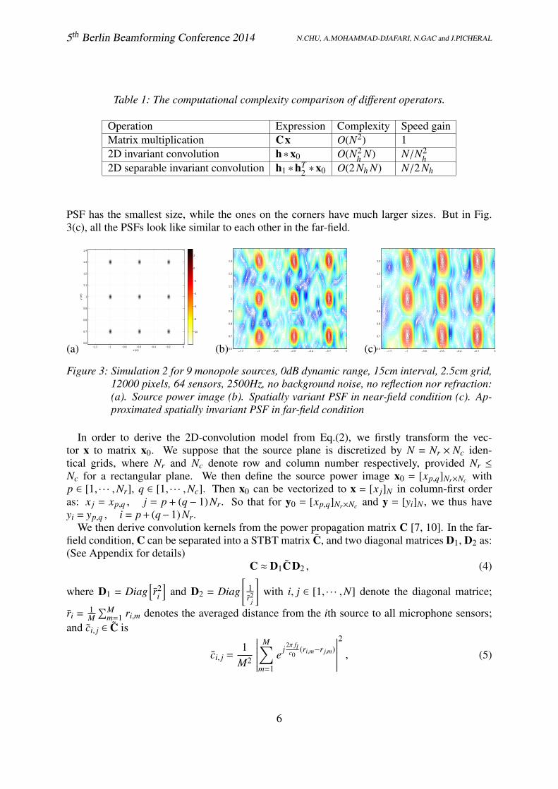
The power propagation model in Eq.(2) reveals that the source power reconstruction can be seenas the image deconvolution from the blurred Beamforming result. However, the Beamformingoften involves in the convolutions with spatially variant kernels. This effect is shown in Fig.3(a-b): same sources produce different shapes of PSFs on different positions, and the center

5


Table 1: The computational complexity comparison of different operators.

Operation Expression Complexity Speed gainMatrix multiplication Cx O(N2) 12D invariant convolution h∗x0 O(N2

h N) N/N2h

2D separable invariant convolution h1 ∗hT2 ∗x0 O(2 Nh N) N/2 Nh

PSF has the smallest size, while the ones on the corners have much larger sizes. But in Fig.3(c), all the PSFs look like similar to each other in the far-field.

(a) x (m)

y (m

)

−1.2 −1 −0.8 −0.6 −0.4 −0.2 00.6

0.7

0.8

0.9

1

1.1

1.2

1.3

1.4

−10

−8

−6

−4

−2

0

2

(b) −1.2 −1 −0.8 −0.6 −0.4 −0.2 00.6

0.7

0.8

0.9

1

1.1

1.2

1.3

(c) −1.2 −1 −0.8 −0.6 −0.4 −0.2 00.6

0.7

0.8

0.9

1

1.1

1.2

1.3

Figure 3: Simulation 2 for 9 monopole sources, 0dB dynamic range, 15cm interval, 2.5cm grid,12000 pixels, 64 sensors, 2500Hz, no background noise, no reflection nor refraction:(a). Source power image (b). Spatially variant PSF in near-field condition (c). Ap-proximated spatially invariant PSF in far-field condition

In order to derive the 2D-convolution model from Eq.(2), we firstly transform the vec-tor x to matrix x0. We suppose that the source plane is discretized by N = Nr × Nc iden-tical grids, where Nr and Nc denote row and column number respectively, provided Nr ≤

Nc for a rectangular plane. We then define the source power image x0 = [xp,q]Nr×Nc withp ∈ [1, · · · ,Nr], q ∈ [1, · · · ,Nc]. Then x0 can be vectorized to x = [x j]N in column-first orderas: x j = xp,q , j = p + (q− 1) Nr. So that for y0 = [xp,q]Nr×Nc and y = [yi]N , we thus haveyi = yp,q , i = p + (q−1) Nr.

We then derive convolution kernels from the power propagation matrix C [7, 10]. In the far-field condition, C can be separated into a STBT matrix C, and two diagonal matrices D1, D2 as:(See Appendix for details)

C ≈ D1CD2 , (4)

where D1 = Diag[r2

i

]and D2 = Diag

[1r2

j

]with i, j ∈ [1, · · · ,N] denote the diagonal matrice;

ri = 1M

∑Mm=1 ri,m denotes the averaged distance from the ith source to all microphone sensors;

and ci, j ∈ C is

ci, j =1

M2

∣∣∣∣∣∣∣M∑

m=1

e j2π flc0

(ri,m−r j,m)

∣∣∣∣∣∣∣2

, (5)

6


Therefore, using Eq.(4) to replace C in the original forward model of Eq.(2), it yields

y = C x + ε , (6)

where y = D−11 y denotes the measured Beamforming power vector with attenuation D−1

1 ; andx = D2 x denotes the source power vector with attenuation D2; and ε = σ2

e D−11 1a denotes the

model errors. Since the averaged distance ri can be easily calculated beforehand, we take x asx and y as y for symbol simplicity in the followings.

According to the STBT matrix C, we can rewrite Eq.(6) by using the 2D convolution modelas:

y = Hx + ε , (7)

where matrix H denotes valid convolution matrix, satisfying:

[Hx]i = [h∗x0]p,q , i = p + (q−1) Nr , (8)

where index [·]i represents the ith item of a vector; index [·]p,q represent the pth row, qth columnitem of a matrix; Nr denotes row size of the source plane. To express convolution kernel h, wewill discuss the spatially-variant and spatially-invariant two cases in this subsection.

3.1. 2D spatially-variant kernel

According to the STBT matrix C in Eq.(6), spatially-variant kernels in Eq.(8) can be derived as[8, 9, 18]:

h =

Nc∑p=1

Nc∑q=1

Dp,q hp,q , (9)

where Dp,q denotes the piecewise constant interpolation function [18], which is non-negativediagonal matrix satisfying

∑Ncp=1

∑Ncq=1 D

p,q = I (identity matrix), and the lth diagonal item is 1if the lth PSF is in the region of (p,q). We call hp,q the spatially-variant kernel, since hp,q variesalong with the convolution output yi ∈ y, i = p + (q−1) Nr in Eq.(7).

According to the expression of C in Eq.(5), each item hp,q(k, l) ∈ hp,q in Eq.(9) is obtainedas: hp,q(k, l) = ci, j ,

i = p + (q−1) Nr , j = i + (bNhr +12 c− k) Nr + b

Nhc +12 c− l

, (10)

where Nhr × Nh

c denotes the kernel size; k ∈ [1, · · · ,Nhr ], l ∈ [1, · · · ,Nh

c ]; operator b·c denotesinteger part.

In brief, hp,q(k, l) is derived from ci, j in three steps: Firstly, hp,q comes from the specificci, j which are on the same row of i = p + (q− 1) Nr in matrix C; Then, the item hp,q(k, l) isderived by specific ci, j on the column j which is determined by the known index i,k, l as shownin Eq.(10); Finally, hp,q should be flipped up-down, left-right according to the definition of 2Dvalid convolution.

7


3.2. 2D invariant kernel

Owing to the STBT matrix C, its middle row (i = bN+12 c) contains most of the useful items of

other rows in C. According to variant kernels in Eq.(10), we can derive an invariant convolutionkernel h = [hk,l] with k, l ∈ [1, · · · ,Nr] from the middle row of C as:{

hk,l = ci, j ,

i = bN+12 c , j = i + (bNr+1

2 c− k) Nr + bNr+1

2 c− l, (11)

where h is can be a Nr ×Nr square matrix, since the STBT matrix C consists of Nr ×Nr squaresubblocks. Compared with the ’variant’ kernel in Eq.(10), the ’invariant’ kernel in Eq.(11) doesnot change along with convolution output yi, i = p + (q−1) Nr, but remains the same i = bN+1

2 c.

4. Simulations for 2D convolution model validation

On simulations, we will show the five following aspects: Approximation errors between STBTmatrix C and power propagation matrix C; Convolution approximated errors for variant, invari-ant and separable kernels, as well as different kernel sizes and forms (square or rectangular);Convolution computational time for different kernels; Acoustic imaging results based on 2Dinvariant convolution model.

The simulation configurations are shown in above figure: there are M = 64 non-uniformmicrophones locating on the vertical plane. d = 2m is the averaged size of microphone array.D = 4.50m is the distance between the microphone plane and source plane. c0 ≈ 340m/s isthe acoustic speed in the common air. T = 10000 is the total number of samplings. For thesimulated sources in Fig.2(a), there are simulated 4 monopoles and 5 complex sources, spacedat least 20cm from each other. Original source powers x∗ are within [0.08,2] ([-10.3,3.7]dB)and 14dB dynamic range. And power image size is of Nc = 27 and Nr = 17 as shown in Fig.2(c).The i.i.d AWGN noise power is set σ2

e = 0.86 (-0.7dB), thus the averaged SNR is 0dB.

4.1. Approximation errors of STBT matrix

(a)

100 200 300 400

50

100

150

200

250

300

350

400

450

0.2

0.4

0.6

0.8

1

(b)

100 200 300 400

50

100

150

200

250

300

350

400

450

0.2

0.4

0.6

0.8

1

(c)

100 200 300 400

50

100

150

200

250

300

350

400

450 0

0.005

0.01

0.015

0.02

0.025

Figure 4: Power propagation matrix and its STBT approximation at 2500Hz: (a) C = [ci, j] (b)C = [ci, j] (c) Approximation error matrix |ci, j− ci, j|

8


In Fig.4, the matrix structures of C = [ci, j] in Eq.(3) and C = [ci, j] in Eq.(5) are quite similarto each other. The biggest relative error of STBT approximation is less than 2.5%. Therefore,the power propagation matrix C can be effectively approximated by the STBT matrix C.

4.2. Convolution approximated errors for different kernels

3 5 7 9 11 13 15 17 19 21 23 25 27−30

−20

−10

0

10

20

30

PSF size

δ 2 (dB

) con

volu

tion

erro

r

Invariant square PSFInvariant rectangular PSFVariant square PSFsVariant rectangular PSFsInvariant PSF 53X33Variant PSFs 53X33Separarble PSFError of Separability PSF

3 5 7 9 11 13 15 17 19 21 23 25 270

3

6

9

12

15

18

Err

or (%

) of s

epar

able

con

volu

tion

← error of separability

Figure 5: Convolution performance comparisons among variant, invariant and separable con-volution kernels at 2500Hz.

We define the convolution approximated errors as δy =‖y−y‖22‖y‖22

× 100%, where y refers to the

Beamforming result using measured signals in Eq.(1) as shown in Fig.2(c); y refers to theconvolution results respectively using variant kernels in Eq.(10) and invariant kernel in Eq.(11).

In Fig.5, we show convolution approximated errors δy versus various kernel sizes. We exam-ine 7 types of kernels with different forms. Firstly, both the variant and invariant kernel with thelargest size of 53× 33 obtain the very small convolution errors, which validates our proposed(in)variant convolution models in Eq.(10) and Eq.(11). Secondly, the larger kernel size is, thesmaller δy becomes, and both the square and rectangular kernels obtain similar δy for each case,so that we can choose the square kernel for simplicity. Thirdly, the invariant kernel obtains assmall δy as those of variant kernels, so that we can use invariant model to effectively approxi-mate power propagation model. Fourthly, when kernel size Nh approaches source power imageNr = 17, all δy of 7 kernels becomes small and remains stable.

4.3. Acoustic imaging via 2D invariant convolution model

In the 2D convolution model of Eq.(6), this linear system of equation with STBT matrixC can be generally solved by multichannel Levinson algorithm [8, 9]. But in order to ob-tain robust source reconstruction in the strong background noises and approximation errors,

9


(a) x (m)

y (m

)

−1.2 −1 −0.8 −0.6 −0.4 −0.2 0

0.6

0.7

0.8

0.9

1

1.1

1.2

1.3

1.4

−12

−10

−8

−6

−4

−2

0

2

(b) x (m)

y (m

)

−1.2 −1 −0.8 −0.6 −0.4 −0.2 0

0.6

0.7

0.8

0.9

1

1.1

1.2

1.3

1.4

−12

−10

−8

−6

−4

−2

0

2

Figure 6: Simulations at 2500Hz, 0dB SNR, 15dB display: (a) Bayesian JMAP method viaconventional forward model (b) Bayesian JMAP method via invariant convolutionmodel

we apply the Bayesian JMAP method proposed in authors’ paper [5] which aims to solveJ(x,θ) = ‖y−Hx− ε‖2 +D(x,θ), where θ denotes prior model parameters; D(·) denotes theregularization using the prior models on the unknowns.

In Fig.2, the Beamforming merely gives some strong source powers. In Fig.6, BayesianJMAP method via classical forward model well detects all source powers except for the weakestmonopole source. The Bayesian JMAP method via convolution model can quickly reconstructmost of the sources, but the recovered source patterns are affected by measured errors.

5. Wind tunnel experiments

Figure 7: Acoustic imaging on the vehicle surface in Wind tunnel S2A.

Figure 7 shows the configurations of the wind tunnel S2A [16], object vehicle, Non-uniformarray and wind refraction. We suppose that all acoustic sources locate on the same plane. Thisassumption is almost satisfied, because the curvature of the car side is relatively small com-pared to the distance D=4.5m between the car and array plane. Since the scanning step is set by∆p = 5cm, the source plane of car side is of 1.5× 5 m2 (31×101 pixels). On the real data, there

10


are T=524288 samplings with the sampling frequency fs=2.56×104 Hz. We separate thesesamplings into I=204 blocks with L=2560 samplings in each bloc. The working frequency is2500Hz which is sensitive to human being. The image results are shown by normalized dBimages with 10dB span. For the actual propagation distance rn,m in Eq.(1), we apply equiv-alent source to make refraction correction, and the mirror source signal to correct the groundreflection as discussed in author’s paper[5].

(a)

−2 −1.5 −1 −0.5 0 0.5 1 1.5 20

0.5

1

−10

−8

−6

−4

−2

0

(a’)

−2 −1.5 −1 −0.5 0 0.5 1 1.5 20

0.5

1

−10

−8

−6

−4

−2

0

(b)

−2 −1.5 −1 −0.5 0 0.5 1 1.5 20

0.5

1

−10

−8

−6

−4

−2

0

(b’)

−2 −1.5 −1 −0.5 0 0.5 1 1.5 20

0.5

1

−10

−8

−6

−4

−2

0

(c)

−2 −1.5 −1 −0.5 0 0.5 1 1.5 20

0.5

1

−10

−8

−6

−4

−2

0

(c’)

−2 −1.5 −1 −0.5 0 0.5 1 1.5 20

0.5

1

−10

−8

−6

−4

−2

0

(d)

−2 −1.5 −1 −0.5 0 0.5 1 1.5 20

0.5

1

−10

−8

−6

−4

−2

0

(d’)

−2 −1.5 −1 −0.5 0 0.5 1 1.5 20

0.5

1

−10

−8

−6

−4

−2

0

Figure 8: Left: real data at 2500Hz (a) vehicle surface (b) Beamforming (c) Bayesian JMAPvia classical forward model (d) JMAP via invariant convolution model. Right: hybriddata (a’) 5 simulated complex sources (b’)-(d’) corresponding methods.

Figure.8(a-d) illustrate the estimated power images of mentioned methods at 2500Hz. Dueto the high sidelobe effect, Beamforming just gives a coarse image of strong sources. TheBayesian JMAP method via sparse prior not only manages to distinguish the strong sourcesaround the two wheels, rearview mirror and side window, but also successfully reconstructs theweek ones on the front cover and light. The Bayesian JMAP method via proposed 2D invariantconvolution model can achieve the source reconstruction as good as the JMAP via conventionalforward model. Figure.8(a’-d’) use the hybrid data which simulated source are added to thereal data. Bayesian via convolution model can further effectively detect both the simulated andoriginal source powers in the real data.

In Table 2, the computation speed is greatly improved by 2D invariant convolution model inEq.(11) compared to conventional model in Eq.(2)

11


Table 2: Computational cost for treating real data of whole car: image 31×101 pixels, at2500Hz, based on CPU: 3.33Hz. ’JMAP+Conv’ is short for Bayesian JMAP methodvia 2D invariant convolution model

Methods CB JMAP JMAP+ConvTime (s) 1 1012 180

6. Conclusions and perspectives

In this paper, we propose a 2D convolution model in Eq.(7) to approximate the forward model ofsource power propagation in Eq.(2), so that proposed Bayesian JMAP method is more quicklycarried out. We firstly discuss the 2D-convolution model using a variant kernel in Eq.(10) andinvariant kernel in Eq.(11) respectively. Convolution kernels (size and item values) are derivedfrom the Symmetric Toeplitz Block Toeplitz (STBT) structure of power propagation matrix.

On simulations, the main conclusions are:

• There are relatively small approximation errors between STBT matrix C and power prop-agation matrix C;

• 2D invariant convolution model successfully approximates the power propagation model;

• 2D invariant kernel whose size is just the half of the source power image efficiently per-forms the 2D convolution model.

• Bayesian JMAP method via 2D invariant convolution model obtains an acceptable imag-ing result compared to the conventional power propagation model;

On real data and hybrid data, we demonstrate that using 2D invariant convolution modelcan greatly accelerate the Bayesian JMAP method and contribute a rapid implementation forindustry application.

However, there are at least three aspects to be further improved:

• The acoustic image quality using the 2D invariant or separable convolution model shouldbe carefully refined, and it is necessary to balance between source reconstruction andcomputational cost, especially for real data treatment of wind tunnel experiments.

• To improve the source estimation results, the model error ε in the proposed convolutionmodel might not be always Gaussian white noise distribution, but probably the spatiallynon-stationary Gaussian distribution on the different parts of source plane or on the dif-ferent microphones.

• For GPU implementation on the large scale of real data in tunnel experiments, it is quiteworthy of optimizing advanced deconvolution algorithms (such as the Bayesian infer-ence) via separable convolution model, so that the peak-power computation of GPU canbe well utilized, and the drawbacks of limited local on-chip memory could be avoided tosome extend.

12


A. STBT Matrix Approximation

(a) (b)

Figure 9: Assumptions for STBT matrix C approximation (a) Approximation for Toeplitz in asubblock (b) Approximation for block Toeplitz block

For the ith source i ∈ [1, · · · ,N], we suppose that there exists an averaged distance ri =1M

∑Mm=1 ri,m from sources to the sensor plane, satisfying ri/ri,m ≈ 1 for any sensor m ∈ [1, · · · ,M].

According to the above assumption, each item ci, j ∈ C in Eq.(3) can be approximated by:

ci, j ≈

∣∣∣∣∣∣∣∣∣1∑M

m=11

r2im

M∑m=1

1rim r jm

e j2π flc0

(rim−r jm)

∣∣∣∣∣∣∣∣∣2

= r2i

1M2

∣∣∣∣∣∣∣M∑

m=1

e j2π flc0

(ri,m−r j,m)

∣∣∣∣∣∣∣2

1r2

j

, (12)

According to Eq.(5), we have

ci, j =1

M2

∣∣∣∣∣∣∣M∑

m=1

e j2π flc0

(ri,m−r j,m)

∣∣∣∣∣∣∣2

, (13)

where rim denotes the propagation distance from ith discrete source (at the position pi on thediscrete source plane) to the mth sensor; fl denotes the lth frequency bin; M is the total numberof sensors; i, j ∈ [1, · · · ,N]; and c0 is the acoustic propagation speed.

According to Eq.(13), we get ci, j = c j,i, C = CT . Therefore, C is a symmetric matrix. And Ccan be expressed by subblock matrices Cq,l as follows: C = [Cq,l]Nc×Nc , Cq,l = [c(q,l)

p,k ]Nr×Nr , c(q,l)p,k = ci, j ∈ C

i = p + (q−1) Nr, j = k + (l−1) Nr(14)

where Cq,l with q, l ∈ [1, · · · ,Nc] denotes the subblock matrix at qth-row and lth-column block ofC; and C has the number of Nc×Nc subbolcks. c(q,l)

p,k with p,k ∈ [1, · · · ,Nr] denotes the pth-rowand kth-column item of Cq,l, and Cq,l has the size of Nr ×Nr.

13


We then suppose that

|ri,m− r j,m| ≈ |ri+1,m− r j+1,m|, bi

Nrc = b

jNrc , (q = l) (15)

where b·c denotes the integer part, which reflects that the ith and jth, i + 1th and j + 1th discretesources are on the same column on the source power image.

Based on Eq.(13), it yields ci, j = ci+1, j+1 for i and j belong to one subblock. Since index iand j are periodically changing, we then have ci, j = ci+Nr, j+Nr in two subblock.

According to Eq.(14) and (15), for any c(q,l)p,k , c(q,l)

p+1,k+1 ∈ Cq,l, we have c(q,l)p+1,k+1 = ci+1, j+1 =

ci, j = c(q,l)p,k . Therefore, subblock Cq,l is a Toeplitz matrix.

For any c(q,l)p,k ∈ Cq,l and c(q+1,l+1)

p,k ∈ Cq+1,l+1, we get c(q+1,l+1)k,l = ci+Nr, j+Nr = ci, j = c(q,l)

p,k , andCq,l = Cq+1,l+1. Therefore, C is a block Toeplitz matrix.

Above all, C is proved ton be a STBT matrix..

References

[1] J. Antoni. “A Bayesian approach to sound source reconstruction: optimal basis, regular-ization, and focusing.” The Journal of the Acoustical Society of America, 131, 2873–2890,2012.

[2] T. Brooks and W. Humphreys. “A Deconvolution Approach for the Mapping of AcousticSources (DAMAS) determined from phased microphone arrays.” Journal of Sound andVibration, 294(4-5), 856–879, 2006. ISSN 0022-460X.

[3] R. H. Chan, J. G. Nagy, and R. J. Plemmons. “FFT-based preconditioners for Toeplitz-block least squares problems.” SIAM journal on numerical analysis, 30(6), 1740–1768,1993.

[4] J. Chen, K. Yao, and R. Hudson. “Source localization and beamforming.” Signal Process-ing Magazine, IEEE, 19(2), 30–39, 2002.

[5] N. Chu, A. Mohammad-Djafari, and J. Picheral. “Robust Bayesian super-resolution ap-proach via sparsity enforcing a priori for near-field aeroacoustic source imaging.” Journalof Sound and Vibration, 332(18), 4369–4389, 2013. ISSN 0022-460X.

[6] R. Dougherty. “Extensions of DAMAS and Benefits and Limitations of Deconvolutionin Beamforming.” In 11th AIAA/CEAS Aeroacoustics Conference, pages 1–13. Monterey,CA, USA, 23-25 May, 2005. ISSN 0146-3705.

[7] R. M. Gray. Toeplitz and circulant matrices: A review. Now Pub, 2006.

[8] P. C. Hansen. “Deconvolution and regularization with Toeplitz matrices.” NumericalAlgorithms, 29(4), 323–378, 2002.

[9] J. Haupt, W. U. Bajwa, G. Raz, and R. Nowak. “Toeplitz compressed sensing matriceswith applications to sparse channel estimation.” Information Theory, IEEE Transactionson, 56(11), 5862–5875, 2010.

14


[10] M. Kac. “Toeplitz matrices, translation kernels and a related problem in probability the-ory.” Duke Mathematical Journal, 21(3), 501–509, 1954.

[11] T. Kailath and J. Chun. “Generalized displacement structure for block-toeplitz, toeplitz-block, and toeplitz-derived matrices.” SIAM Journal on Matrix Analysis and Applications,15(1), 114–128, 1994.

[12] J. Lanslots, F. Deblauwe, and K. Janssens. “Selecting Sound Source Localization Tech-niques for Industrial Applications.” Sound and Vibration, 44(6), 6–10, 2010. ISSN 1541-0161.

[13] S. Lehman and A. Devaney. “Transmission mode time-reversal super-resolution imaging.”The Journal of the Acoustical Society of America, 113(5), 2742–2753, 2003.

[14] A. Massa and G. Oliveri. “Bayesian compressive sampling for pattern synthesis withmaximally sparse non-uniform linear arrays.” IEEE Transactions on Antennas and Prop-agation, 59(10), 467–681, 2011.

[15] J. D. Maynard, E. G. Williams, and Y. Lee. “Nearfield acoustic holography: I. Theory ofgeneralized holography and the development of NAH.” 78(4), 1395–1413, 1985. ISSN00014966.

[16] A. Menoret, N. Gorilliot, and J.-L. Adam. “Acoustic imaging in wind tunnel S2A.” In10th Acoustics conference (ACOUSTICS2010). Lyon, France, 2010.

[17] A. B. Nagy. “Aeroacoustics research in Europe: The CEAS-ASC report on 2010 high-lights.” Journal of Sound and Vibration, 330(21), 4955–4980, 2011.

[18] J. G. Nagy and D. P. O’leary. “Fast iterative image restoration with a spatially varying psf.”In Optical Science, Engineering and Instrumentation’97, pages 388–399. InternationalSociety for Optics and Photonics, 1997.

[19] A. Tarantola. Inverse problem theory and methods for model parameter estimation. Soci-ety for Industrial Mathematics, 2005.

[20] Y. Wang, J. Li, P. Stoica, M. Sheplak, and T. Nishida. “Wideband RELAX and widebandCLEAN for aeroacoustic imaging.” Journal of Acoustical Society of America, 115(2),757–767, 2004. ISSN 00014966.

15

2D convolution model using (in)variant kernels for fast ...

Documents

Transcript of 2D convolution model using (in)variant kernels for fast ...