Energy Procedia 45 ( 2014 ) 131 – 140

1876-6102 © 2013 The Authors. Published by Elsevier Ltd. Open access under CC BY-NC-ND license.Selection and peer-review under responsibility of ATI NAZIONALEdoi: 10.1016/j.egypro.2014.01.015

ScienceDirect

68th Conference of the Italian Thermal Machines Engineering Association, ATI2013

2D CFD Modeling of H-Darrieus Wind Turbines using a Transition Turbulence Model

Rosario Lanzafame, Stefano Mauro*, Michele Messina

Department of Industrial Engineering, University of Catania, Viale A. Doria 6, 95125, Catania, Italy

Abstract

In the present paper, the authors describe the strategy to develop a 2D CFD model of H-Darrieus Wind Turbines. The model was implemented in ANSYS Fluent solver to predict wind turbines performance and optimize its geometry. As the RANS Turbulence Modeling plays a strategic role for the prediction of the flowfield around wind turbines, different Turbulence Models were tested. The results demonstrate the good capabilities of the Transition SST turbulence model compared to the classical fully turbulent models. The SST Transition model was calibrated modifying the local correlation parameters through a series of CFD tests on aerodynamic coefficients of wind turbines airfoils. The results of the tests were implemented in the 2D model of the wind turbine.The computational domain was structured with a rotating ring mesh and the unsteady solver was used to capture the dynamic stall phenomena and unsteady rotational effects. Both grid and time step were optimized to reach independent solutions. Particularly a high quality 2D mesh was obtained using the ANSYS Meshing tool while a Sliding Mesh Model was used to simulate rotation.Spatial discretization algorithm, interpolation scheme, pressure - velocity coupling and turbulence boundary condition wereoptimized also. The 2D CFD model was calibrated and validated comparing the numerical results with two different type of H-Darrieusexperimental data, available in scientific literature. A good agreement between numerical and experimental data was found. The present work represents the basis to develop an accurate 3D CFD unsteady model and may be used to validate the simplest 1D models and support wind tunnel experiments.

© 2013 The Authors. Published by Elsevier Ltd. Selection and peer-review under responsibility of ATI NAZIONALE.

Keywords: H-Darrieus Wind Turbine; CFD; Transition Turbulence Modeling; URANS; VAWT performance prediction.

* Corresponding author. Tel.: +39 095 7382414; fax: +39 095 337994.E-mail address: mstefano@diim.unict.it (S. Mauro)

Available online at www.sciencedirect.com

© 2013 The Authors. Published by Elsevier Ltd. Open access under CC BY-NC-ND license.Selection and peer-review under responsibility of ATI NAZIONALE

132 Rosario Lanzafame et al. / Energy Procedia 45 ( 2014 ) 131 – 140

Nomenclature

Cp Mean Power Coefficient [-] λ Tip Speed Ratio [-] Tl Mean Torque per unit length [N] Cl Lift Coefficient [-] y+ Dimensionless wall distance [-] Cd Drag Coefficient [-] Tu Turbulent Intensity [%] Cm Moment Coefficient per unit length [m-1] Re Reynolds Number [-] L Blade length [m] c Chord [m] R Rotor Radius [m] n Rotational speed [r/min] Vw Wind Speed [m/s] γ Intermittency [-] Δn Angular Step [deg] Reθt Transition Reynolds Number [-] Δt Time step [s] l Fluent unit length [m] Flength Transition region length parameter [-] S Fluent unit surface [m2] Reθc Critical Transition Reynolds Number [-]

1. Introduction

Vertical Axis Wind Turbines (VAWTs) are becoming ever more important in wind power generation thanks to its compactness and adaptability for domestic installations. However, it is well known that VAWTs have lower efficiency, above all if compared to HAWTs. To improve VAWTs performance, industries and researchers are trying to optimize the design of the rotors. Some numerical codes like Vortex Method or Multiple Streamtube Model [1-8] have been developed to predict VAWTs performance and optimize efficiency but these codes are based on 1D simplified equations and they need accurate experimental data for aerodynamic coefficients of the airfoils. Furthermore they do not provide information on the wakes and they use semi empirical equations to predict effects like tip vortex and dynamic stall. These codes are so mainly used to do a first attempt design and the results have to be validated using wind tunnel experiments. However, as the wind tunnel experiments are expensive in terms of both costs and time, another way to study aerodynamic behavior of the rotors is to use CFD.

As it is known, CFD resolves the fluid dynamic equations and it is certainly more realistic than the 1D models but there are many other problematic issues like stall and turbulence modeling, unsteady rotational effects and long computation time. Some works were found in scientific literature [9-14] regarding the application of CFD modeling on VAWTs. The problem in general was the power overestimation due to the arduous prediction of stall phenomena using fully turbulent RANS models for low Reynolds numbers.

In this paper the authors present the strategy of generating a 2D CFD model to predict H-Darrieus rotors performance and solve such issues.

Particularly, the CFD model was developed using ANSYS Workbench 14.5 multi-physics platform. Two different type of experimental rotors were simulated to calibrate and validate the model. The first of which is a 3 blades rotor with NACA 0015 symmetrical airfoil while the second is a 3 blades rotor with NACA 4518 asymmetrical airfoil in order to validate the model for different airfoils [15,16].

First step was to generate a simplified CAD and optimize the computational domain. Then a grid independent solution study was done, refining the mesh till the results obtained with different grids were negligible [25,26]. The most important part of the work was to optimize the SST Transition turbulence model, modifying the local correlation parameters through a series of 2D CFD tests on wind turbine airfoils [17-24]. As the unsteady rotational effects are very important in VAWTs, an unsteady Sliding Mesh Model with non conformal mesh was used. Time step of the transient model was optimized also [25-26].

Simulations were performed on a Fujitsu Primergy TX200 S5 Server, with 2 Intel Quad Core Xeon X5570 processors (2.93 GHz) and 48 GB of RAM memory installed. A parallel computing technique was implemented in ANSYS Fluent solver.

A comparison between fully turbulent SST k-ω turbulence model and SST Transition model was done to demonstrate the superior capability of the modified Transition model to predict VAWTs performance and underline the important role of laminar to turbulent transition modeling.

The use of the URANS (Unsteady Reynolds Averaged Navier Stokes) Transition model leads to a good prediction of trend of mechanical power and power coefficient with an overestimation of 6-8 % due to the well known limits of the 2D models that do not take into account the 3D effects like tip vortex. This problem will be investigated in a 3D CFD model that will be developed in the future.

Rosario Lanzafame et al. / Energy Procedia 45 ( 2014 ) 131 – 140 133

2. CFD numerical model

The process of generating the 2D CFD model was done inside the ANSYS Workbench multi-physics platform where it is possible to develop a workflow, starting from CAD generation to post-processing of the results. Particularly, the Finite Volume Fluent Solver was used in an Unsteady RANS (URANS) version to solve the Navier-Stokes equations and capture the unsteadiness like the continuous change in the aerodynamic angle of the blade with rotation.

The workflow of the model was as follow: Generation of a simplified 2D CAD and computational domain; High quality meshing of the domain to meet the specifics of the turbulence models and reach grid

independent solutions; Setting the Fluent Solver and calibrating the model; Optimization of the Transition Turbulence model; Post-processing results;

2.1. Experimental rotors features

Two different type of Straight-bladed VAWT rotors, founded in scientific literature [15-16], were used to develop and validate the 2D CFD model. The features are listed in the table below (Tab. 1). For simplicity, the rotors will be named as rotor A and rotor B:

Table 1. Experimental rotors features

Rotor type Rotor A Rotor B

Number of blades [-] 3 3

Blade Airfoil [-] NACA 0015 NACA 4518

Blade length (L) [m]

Blade chord (c) [m]

Radius (R) [m]

Rotational speed (n) [r/min]

Wind speed (Vw) [m/s]

Tip Speed Ratio (λ) [-]

3

0.4

1.25

20 - 150

6 - 16

0.2 - 2.2

0.7

0.1

0.3

100 - 625

6 - 18

0.3 - 2.3

These rotors were chosen to generalize the CFD model for different geometrical dimensions and different airfoils.

As there are no provided information on the shaft, the CAD of the rotors were simplified eliminating the shaft and representing only the blades. The experimental data were extrapolated in terms of Cp versus λ curves to correctly compare numerical results with experimental one.

2.2. Computational domain generation and optimization

Generating the right computational domain for a Fluid Dynamic problem is an important task of the modeling process. It is necessary to take into account different requirements [26,27].

First of all, the domain should not be too small to correctly reproduce the flow around the rotor and it should not be too large to not uselessly increase cells number of the grid and hence computation time. Furthermore, the domain has to be suitable for adequately reproduce the rotation. At last it has to be taken into account the requirements of the meshing in terms of quality and first cell positioning near the blades. The advanced turbulence models used in this work need a very fine mesh near the wall so that y+ < 1 [19-23]. Also important is to define the correct boundary condition for the physical problem to reproduce.

Some tests were performed to achieve the optimal compromise. The computational domain was generated using the CAD interface ANSYS "Design Modeler". Different domains were meshed and then tested with the default

134 Rosario Lanzafame et al. / Energy Procedia 45 ( 2014 ) 131 – 140

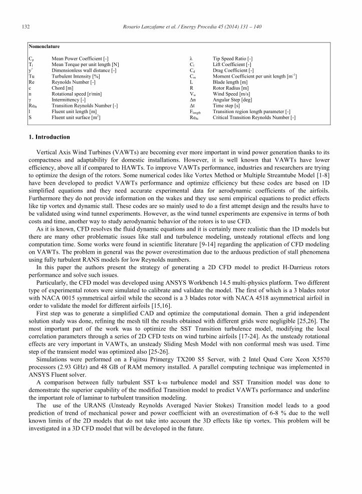
parameters in Fluent. The best compromise was found in a box with a rotating ring that reproduces the rotation. The dimensions of the domain were optimized for the rotor A and then the same criteria were applied to the rotor B (Fig. 1). The domain has 3 separated sub-domains in order to use the Unsteady Sliding Mesh Model. Only the ring is in motion while the box and the interior circle are stationary. The rotating ring has to be as small as possible in the radial direction so that the mesh motion does not modify the real flow-field of the wake.

Boundary conditions (BCs) were defined also. A WALL type BC was used for blades; the line on the left of the box was defined as a VELOCITY INLET type BC; the line on the right of the box was defined as a PRESSURE OUTLET type BC; a SYMMETRY type BC was used for lateral lines of the box. The Symmetry BC is useful because it allows the solver to consider the wall as part of a larger domain, like a ‘free shear slip wall’, avoiding in this way the wall effects [18,25-26]. Finally it can substantially reduce the size of the box. Furthermore, an INTERFACE type BC was used for the contact region between the 3 sub-domains (Fig. 1).

Fig. 1 Computational domain and Boundary Conditions

The rotor was placed five radius from the inlet and eighteen radius from the outlet to correctly reproduce the wake effect. The use of the symmetry BCs allow to reduce the distance from the lateral wall as the rotor was placed only four radius from it. It was verified that using too great a domain would not leads to better results but only to an increase in cell numbers and hence in computational time.

2.3. Mesh generation and optimization

To obtain high quality spatial discretization the three sub-domains were meshed separately but consistently in the interface zone. First of all the attention was placed to mesh the rotating ring where all the most important flow effects take place.

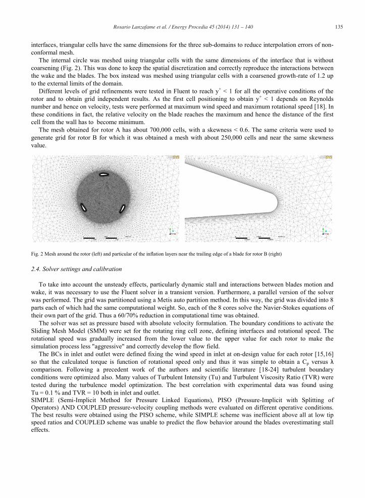
High quality non conformal unstructured mesh was generated for rotor A using ANSYS Meshing advanced sizing functions. Particularly an inflation tool was used to generate 20 levels of quadrangular cells (Fig. 2) in the boundary layer of the blades so that y+ < 1 as required by turbulence models [19-22] and with a growth rate of 1,1. Triangular cells were used outside the boundary layer with the same growth rate up to the inside and outside interface. At the

Rosario Lanzafame et al. / Energy Procedia 45 ( 2014 ) 131 – 140 135

interfaces, triangular cells have the same dimensions for the three sub-domains to reduce interpolation errors of non-conformal mesh.

The internal circle was meshed using triangular cells with the same dimensions of the interface that is without coarsening (Fig. 2). This was done to keep the spatial discretization and correctly reproduce the interactions between the wake and the blades. The box instead was meshed using triangular cells with a coarsened growth-rate of 1.2 up to the external limits of the domain.

Different levels of grid refinements were tested in Fluent to reach y+ < 1 for all the operative conditions of the rotor and to obtain grid independent results. As the first cell positioning to obtain y+ < 1 depends on Reynolds number and hence on velocity, tests were performed at maximum wind speed and maximum rotational speed [18]. In these conditions in fact, the relative velocity on the blade reaches the maximum and hence the distance of the first cell from the wall has to become minimum.

The mesh obtained for rotor A has about 700,000 cells, with a skewness < 0.6. The same criteria were used to generate grid for rotor B for which it was obtained a mesh with about 250,000 cells and near the same skewness value.

Fig. 2 Mesh around the rotor (left) and particular of the inflation layers near the trailing edge of a blade for rotor B (right)

2.4. Solver settings and calibration

To take into account the unsteady effects, particularly dynamic stall and interactions between blades motion and wake, it was necessary to use the Fluent solver in a transient version. Furthermore, a parallel version of the solver was performed. The grid was partitioned using a Metis auto partition method. In this way, the grid was divided into 8 parts each of which had the same computational weight. So, each of the 8 cores solve the Navier-Stokes equations of their own part of the grid. Thus a 60/70% reduction in computational time was obtained.

The solver was set as pressure based with absolute velocity formulation. The boundary conditions to activate the Sliding Mesh Model (SMM) were set for the rotating ring cell zone, defining interfaces and rotational speed. The rotational speed was gradually increased from the lower value to the upper value for each rotor to make the simulation process less "aggressive" and correctly develop the flow field.

The BCs in inlet and outlet were defined fixing the wind speed in inlet at on-design value for each rotor [15,16] so that the calculated torque is function of rotational speed only and thus it was simple to obtain a Cp versus λ comparison. Following a precedent work of the authors and scientific literature [18-24] turbulent boundary conditions were optimized also. Many values of Turbulent Intensity (Tu) and Turbulent Viscosity Ratio (TVR) were tested during the turbulence model optimization. The best correlation with experimental data was found using Tu = 0.1 % and TVR = 10 both in inlet and outlet. SIMPLE (Semi-Implicit Method for Pressure Linked Equations), PISO (Pressure-Implicit with Splitting of Operators) AND COUPLED pressure-velocity coupling methods were evaluated on different operative conditions. The best results were obtained using the PISO scheme, while SIMPLE scheme was inefficient above all at low tip speed ratios and COUPLED scheme was unable to predict the flow behavior around the blades overestimating stall effects.

136 Rosario Lanzafame et al. / Energy Procedia 45 ( 2014 ) 131 – 140

A Second Order Upwind spatial discretization algorithm was used for all the equations (pressure, momentum, and turbulence) and a Least Squares Cell Based algorithm was used for gradients. A Second Order Implicit Formulation was used for Transient algorithm. It is well known that these second order algorithms lead to best results because they considerably reduce interpolation errors and false numerical diffusion [25,26].

At the beginning, every simulation was performed decreasing the Under-Relaxation Factors to facilitate the convergence. To obtain final solutions, the Under-Relaxation Factors were gradually increased to the default values [26].

Four control monitors of the iterative process were defined to check convergence: a monitor for the residuals of the iterative process for the equations solved (momentum, continuity and turbulence); a monitor for the lift coefficient on blades; a monitor for the dynamic pressure on the rotor and another monitor for the momentum coefficient of the rotor. The simulation process was considered to be converged when the residuals decrease under a value of 10-3 and, at the same time, other monitors present a constant oscillating trend typical for the transient simulations. Particularly, to obtain a mean torque value and compare it with experimental data, after reaching convergence, the momentum coefficients were sampled for two revolutions of the rotors. The mass flow balance between inlet and outlet was verified also.

Because of the great variation of rotational speed and the complexity of the flow field, it was impossible to establish a priori an optimal time step for the transient solver. Above all at high rotational speed and high wind speed the time step should be very little to adequately simulate rotation and capture the little time scale of turbulence. Moreover the time step influences the numerical iterative process of the solver, that means that too great a time step leads to unphysical results, while too little a time step leads to great increase in computation time. Basing on these considerations, time step was optimized performing several simulations at different rotational speed for both rotors. A first attempt value was fixed considering the angular velocity. Establishing an angular step of 1° [9] it was calculated the relative time step as follows:

For rotor A, being maximum rotational speed n = 150 r/min:

(1) So the first attempt time step value for rotor A was Δt = 10-3 s. For rotor B, being maximum rotational speed n = 600 r/min:

(2) So the first attempt time step value for rotor B was Δt = 3 · 10-4 s. As these time step values did not meet the convergence criteria and led to bad results compared to experimental

data, they were gradually decreased till the solution was converged and the results using two consecutive time steps were negligible. Optimal time steps were Δt = 5 · 10-4 s for rotor A and Δt = 1 · 10-4 s for rotor B

2.5. Transition Turbulence model optimization

The most problematic issue using CFD for modeling airfoil behavior at low Reynolds number is to capture the stall phenomena. This is a well known problem and it is mainly due to the inefficiency of RANS turbulence models to capture the boundary layer separation caused by adverse pressure gradient. Above all at low Re, an important part of the boundary layer is laminar so, the use of a classical fully turbulent model does not adequately predict the real boundary layer behavior. Laminar boundary layer in fact is quite sensitive to adverse pressure gradient and this leads to an earlier separation if compared to a turbulent boundary layer and, ultimately, in an unphysical simulation of the incipient and deep stall. As the VAWTs work at low Re, stall phenomena are of crucial importance for their modeling. For this reason, the use of a calibrated transition model should lead to a more realistic prediction of the airfoils aerodynamic behavior [18-20,23] and consequently a better prediction of the VAWTs performance.

In the present work, the SST Transition Turbulence model was used. This model is based on SST k-ω transport equations [24] coupled with two additional transport equations, one for intermittency γ and one for the Transition

Rosario Lanzafame et al. / Energy Procedia 45 ( 2014 ) 131 – 140 137

Reynolds number Reθt. These additional equations were implemented by Menter et al. [21] who used some proprietary empirical correlations to allow proper closure of the model. The empirical correlations control boundary layer transition from laminar to turbulent and were calibrated through experimental test cases on flat plates [22-23].

As the default model was not able to adequately predict the rotor’s performance, the idea was to calibrate the local correlation parameters through a series of 2D CFD tests on wind turbine airfoils and to use these optimal correlation parameters for the CFD model of VAWTs [18].

In order to calibrate the SST Transitional model for wind turbine applications, a long process of optimizing the local correlation variables was carried out. Several simulations on typical wind turbine airfoils [17] (NACA 0012, NACA 63415, etc.) were performed using Fluent. Inlet and outlet turbulence boundary conditions were also optimized (Tu and TVR).

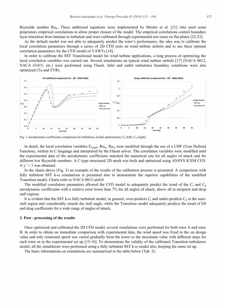
Fig. 3 Aerodynamic coefficients comparison for turbulence model optimization, Cl (left), Cd (right) In detail, the local correlation variables Flength, Reθc, Reθt were modified through the use of a UDF (User Defined

Function), written in C language and interpreted by the Fluent solver. The correlation variables were modified until the experimental data of the aerodynamic coefficients matched the numerical one for all angles of attack and for different low Reynolds numbers. A C-type structured 2D mesh was built and optimized using ANSYS ICEM CFD. A y+ < 1 was obtained.

In the charts above (Fig. 3) an example of the results of the calibration process is presented. A comparison with fully turbulent SST k-ω simulations is presented also to demonstrate the superior capabilities of the modified Transition model. Charts refer to NACA 0012 airfoil.

The modified correlation parameters allowed the CFD model to adequately predict the trend of the Cl and Cd aerodynamic coefficients with a relative error lower than 7% for all angles of attack, above all in incipient and deep stall regions.

It is evident that the SST k-ω fully turbulent model, in general, over-predicts Cl and under-predicts Cd in the near-stall region and considerably retards the stall angle, while the Transition model adequately predicts the trend of lift and drag coefficients for a wide range of angles of attack.

3. Post - processing of the results

Once optimized and calibrated the 2D CFD model, several simulations were performed for both rotor A and rotor B. In order to obtain an immediate comparison with experimental data, the wind speed was fixed to the on design value and only rotational speed was varied gradually from the lower to the maximum value with different steps for each rotor as in the experimental set up [15-16]. To demonstrate the validity of the calibrated Transition turbulence model, all the simulations were performed using a fully turbulent SST k-ω model also, keeping the same set up.

The basic informations on simulations are summarized in the table below (Tab. 2):

138 Rosario Lanzafame et al. / Energy Procedia 45 ( 2014 ) 131 – 140

Table 2. Simulations data

Rotor type Rotor A Rotor B

Wind speed (Vw) [m/s] 10 8

Initial rotational speed (n) [r/min] 20 100

Rotational speed step (Δn) [r/min] 6.5 50

Optimal time step (Δt) [s]

Total simulations [-]

5·10-4

20

1·10-4

12

Total cells number [-] 700,000 250,000

Mean time to convergence [hours] 22 8

Fig.4 Power Coefficient comparison for rotor A (left) and rotor B (right)

As Fluent 2D results were in terms of dimensionless moment coefficient per unit length, after reaching

convergence, the calculated torque was obtained sampling this coefficient for two revolutions and averaging it. In detail, being Tl the calculated torque per unit length:

(3)

Where ρ is the air density (1.225 kg/m3); Cm is the average moment coefficient per unit length calculated by

Fluent; Vw is the fixed wind speed; l is the unit length; S is the unit surface. The total torque was obtained multiplying Tl and the length of the blade L.

In this way a mean Cp was obtained for each simulation and it was compared with experimental data as in the charts above (Fig. 4). As can be seen, the fully turbulent SST k-ω model presents great inaccuracy with an important overestimation and a different trend while the modified Transition SST model follows very well the trend of the experimental data. The little overestimation of the Transition model is mainly due to the limits of a 2D modelization that does not take into account 3D effects like tip vortex and irregular pressure distribution along a 3D blade [9-14]. This will be investigated in future research.

As the 2D CFD calculation results are in good agreement with experimental data the methodology for generating and optimizing the 2D CFD model is considered to be a valid tool to investigate the VAWTs performance and it will be used together with wind tunnel experiments to validate rotors design and as the basis to develop a more accurate 3D CFD model.

Some post-processing images are presented below (Figs. 5-6).

Rosario Lanzafame et al. / Energy Procedia 45 ( 2014 ) 131 – 140 139

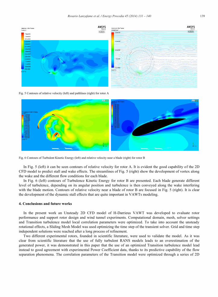
Fig. 5 Contours of relative velocity (left) and pathlines (right) for rotor A

Fig. 6 Contours of Turbulent Kinetic Energy (left) and relative velocity near a blade (right) for rotor B In Fig. 5 (left) it can be seen contours of relative velocity for rotor A. It is evident the good capability of the 2D

CFD model to predict stall and wake effects. The streamlines of Fig. 5 (right) show the development of vortex along the wake and the different flow conditions for each blade.

In Fig. 6 (left) contours of Turbulence Kinetic Energy for rotor B are presented. Each blade generate different level of turbulence, depending on its angular position and turbulence is then conveyed along the wake interfering with the blade motion. Contours of relative velocity near a blade of rotor B are focused in Fig. 5 (right). It is clear the development of the dynamic stall effects that are quite important in VAWTs modeling.

4. Conclusions and future works

In the present work an Unsteady 2D CFD model of H-Darrieus VAWT was developed to evaluate rotor performance and support rotor design and wind tunnel experiments. Computational domain, mesh, solver settings and Transition turbulence model local correlation parameters were optimized. To take into account the unsteady rotational effects, a Sliding Mesh Model was used optimizing the time step of the transient solver. Grid and time step independent solutions were reached after a long process of refinement.

Two different experimental rotors, founded in scientific literature, were used to validate the model. As it was clear from scientific literature that the use of fully turbulent RANS models leads to an overestimation of the generated power, it was demonstrated in this paper that the use of an optimized Transition turbulence model lead instead to good agreement with experimental Power Coefficient data, thanks to its predictive capability of the flow separation phenomena. The correlation parameters of the Transition model were optimized through a series of 2D

140 Rosario Lanzafame et al. / Energy Procedia 45 ( 2014 ) 131 – 140

CFD tests on typical wind turbine airfoils using a UDF written in C language. The optimal local variables were then transferred in the CFD model of the rotor. The same simulations were performed using a fully turbulent SST k-ω model to demonstrate the superior predictive capabilities of the modified Transition model. Only a slight overestimation was denoted for the Transition model and this is due to the limits of a 2D modelization that does not take into account 3D effects (i.e. tip vortex). For this reason the authors will use this methodology to develop a 3D CFD model in the future research and assesses whether improvements justify the great increase of calculation time.

However, considering the good predictive results of the 2D CFD model, this will be used in the future to support experiments in the proprietary sub-sonic wind tunnel and to validate design optimization.

References

[1] Strickland J.H. The Darrieus turbine: a performance prediction model using multiple streamtube. 1975. SAND 75-0431. [2] Paraschivoiu I. Double-Multiple streamtube model for Studying vertical-axis wind turbines. J Propulsion Power July August 1988;4:4 [3] Paraschivoiu I. Wind turbine design: with empasis on darrieus concept. Montreal: Polytechnic International Press; 2002 [4] Beri H., Yao Y. Double Multiple Stream Tube Model and Numerical Analysis of Vertical Axis Wind Turbine. Energy and Power

Engineering, 2011, 3, 262-270 [5] Paraschivoiu I., Saeed F., Desobry V. Prediction capabilities in vertical axis wind turbine aerodynamics. The World Wind Energy Conference

and Exhibition, Berlin, Germany, 2-6 July 2002 [6] Strickland, J. H., Webster B. T., Nguyen T. A Vortex Model of the Darrieus Turbine: An Analytical and Experimental Study. Transaction of

the ASME 500/Vol. 101, December 1979 [7] Wang L. B., Zhang L., Zeng N. D. A potential flow 2-D vortex panel model: Applications to vertical axis straight blade tidal turbine. Energy

Conversion and Management 48 (2007) 454–461 [8] Strickland J. H., Brownlee B. G. A Vortex model for the Vertical Axis Wind Turbine. Master Thesis in mechanical Engineer. Texas Tech

University. 1988 [9] Raciti Castelli M., Englaro A., Benin E. The Darrieus wind turbine: Proposal for a new performance prediction model based on CFD. Energy

36 (2011) 4919-4934 [10] Biadgo A. M., Simonovic A., Komarov D., Stupar S. Numerical and Analytical Investigation of Vertical Axis Wind Turbine. FME

Transactions (2013) 41, 49-58 [11] Sabaeifard P.,Razzaghi H., Forouzandeh A. Determination of Vertical Axis Wind Turbines Optimal Configuration through CFD

Simulations. 2012 International Conference on Future Environment and Energy IPCBEE vol.28 [12] Vassberg J. C., Gopinath A.K., Jameson A. Revisiting the vertical-axis wind turbine design using advanced computational fluid dynamics.

AIAA Paper; 2005:0047. 43rd AIAA ASM, Reno, NV. [13] Gupta R., Biswas A. Computational fluid dynamics analysis of a twisted three-bladed H-Darrieus rotor. Journal of Renewable and

Sustainable Energy 2, 043111 _2010_ [14] Simao Ferreira C.J., Bijl H., Van Bussel G., Van Kuik G. Simulating dynamic stall in a 2D VAWT: modeling strategy, verification and

validation with particle image velocimetry data. The Science of making torque from wind. J Phys Conf Ser 2007;75 [15] Bravo R., Tullis S., Ziada S. Performance Testing of a Small Vertical-Axis Wind Turbine. Mechanical Engineering Department, McMaster

University [16] Takao M., Kuma H., Maeda T., Kamada Y., Oki M., Minoda A. A Straight-bladed Vertical Axis Wind Turbine with a Directed Guide Vane

Row - Effect of Guide Vane Geometry on the Performance - Journal of Thermal Science Vol.18, No.1 (2009) 54−57 [17] Sheldal, R. E., Klimas, P. C., Aerodynamic characteristics of Seven symmetrical airfoil sections through 180-degree angle of attack for use in

aerodynamic analysis of vertical axis wind turbines. 1980. SAND 80-2114 [18] Lanzafame R., Mauro S., Messina M. Wind turbine CFD modeling using a correlation-based transitional model. Renewable Energy 52

(2013) 31 - 39 [19] Langtry RB, Gola J, Menter FR. Predicting 2D airfoil and 3D wind turbine rotor performance using a transition model for general CFD

codes. 44th AIAA aerospace sciences meeting and exhibit; 9-12 January, 2006. Reno, Nevada. [20] Menter FR, Kuntz M, Langtry R. Ten years of industrial experience with the SST turbulence model. Flow Turbulence and Combustion

2006;77:277 - 303 [21] Langtry R.B., Menter F.R., Likki S.R., Suzen Y.B., Huang P.G., Völker S. A correlationbased transition model using local variables part I:

model formulation; 2006. Vienna, ASME Paper No. ASME-GT 2004 - 53452. [22] Langtry R.B., Menter F.R., Likki S.R., Suzen Y.B., Huang P.G., Völker S. A correlationbased transition model using local variablesdpart II:

test cases and industrial applications. ASME Journal of Turbomachinery 2006;128(3):423-34 [23] Sørensen N. CFD modelling of laminar-turbulent transition for airfoils and rotors using the γ e Reθ model. Wind Energy 2009; 12:715-33. [24] Wilcox D. C. Turbulence modeling for CFD. DWC industries. [25] Ferziger J.H., Peric M. Computational methods for fluid dynamics. Springer. [26] Blazek J. Computational Fluid Dynamics: Principles and Applications. Second Edition. Elsevier