
290 IEEE TRANSACTIONS ON SIGNAL AND … · grant. The work of M. Pesavento was supported by the...
16
290 IEEE TRANSACTIONS ON SIGNAL AND INFORMATION PROCESSING OVER NETWORKS, VOL. 2, NO. 3, SEPTEMBER 2016 An Online Parallel Algorithm for Recursive Estimation of Sparse Signals Yang Yang, Member, IEEE, Marius Pesavento, Member, IEEE, Mengyi Zhang, Member, IEEE, and Daniel P. Palomar, Fellow, IEEE Abstract—In this paper, we consider a recursive estimation prob- lem for linear regression where the signal to be estimated admits a sparse representation and measurement samples are only se- quentially available. We propose a convergent parallel estimation scheme that consists of solving a sequence of 1 -regularized least- square problems approximately. The proposed scheme is novel in three aspects: 1) all elements of the unknown vector variable are updated in parallel at each time instant, and the convergence speed is much faster than state-of-the-art schemes which update the el- ements sequentially; 2) both the update direction and stepsize of each element have simple closed-form expressions, so the algorithm is suitable for online (real-time) implementation; and 3) the stepsize is designed to accelerate the convergence but it does not suffer from the common intricacy of parameter tuning. Both centralized and distributed implementation schemes are discussed. The attractive features of the proposed algorithm are also illustrated numerically. Index Terms—LASSO, linear regression, minimization stepsize rule, parallel algorithm, recursive estimation, sparse signal pro- cessing, stochastic optimization. I. INTRODUCTION S IGNAL estimation has been a fundamental problem in a number of scenarios, such as wireless sensor networks (WSN) and cognitive radio (CR). WSN has received a lot of attention and is found application in diverse disciplines such as environmental monitoring, smart grids, and wireless communi- cations [2]. CR appears as an enabling technique for flexible Manuscript received March 17, 2015; revised September 15, 2015 and Febru- ary 14, 2016; accepted April 19, 2016. Date of publication May 02, 2016; date of current version August 05, 2016. The work of Y. Yang was supported by the Seventh Framework Programme for Research of the European Commission under Grant ADEL-619647, the EXPRESS project within the DFG priority program CoSIP (DFG-SPP 1798), and the Hong Kong RGC 16207814 research grant. The work of M. Pesavento was supported by the Seventh Framework Pro- gramme for Research of the European Commission under Grant ADEL 619647 and the EXPRESS project within the DFG priority program CoSIP (DFG-SPP 1798). The work of M. Zhang and D. P. Palomar was supported by the Hong Kong RGC 16207814 research grant. The material in this paper was presented at the Asilomar Conference on Signals, Systems, and Computers, Pacific Grove, CA, USA, November 2014 [1]. The associate editor coordinating the review of this manuscript and approving it for publication was Prof. C´ edric Richard. Y. Yang is with the Intel Deutschland GmbH, Neubiberg 85579, Germany (e-mail: [email protected]). M. Pesavento is with the Communication Systems Group, Darmstadt Uni- versity of Technology, Darmstadt 64283, Germany (e-mail: pesavento@nt. tu-darmstadt.de). M. Zhang is with the Department of Computer Science and Engi- neering, The Chinese University of Hong Kong, Hong Kong (e-mail: [email protected]). D. P. Palomar is with the Department of Electronic and Computer Engineer- ing, The Hong Kong University of Science and Technology, Kowloon, Hong Kong (e-mail: [email protected]). Color versions of one or more of the figures in this paper are available online at http://ieeexplore.ieee.org. Digital Object Identifier 10.1109/TSIPN.2016.2561703 and efficient use of the radio spectrum [3], [4], since it allows unlicensed secondary users (SUs) to access the spectrum pro- vided that the licensed primary users (PUs) are idle, and/or the interference generated by the SUs is below a certain level that is tolerable for the PUs [5], [6]. One prerequisite in CR systems is the ability to obtain a pre- cise estimate of the PUs’ power distribution map so that the SUs can avoid the areas in which the PUs are actively trans- mitting. This is usually realized through the estimation of the position, transmit status, and/or transmit power of PUs [7]–[10], and the estimation is typically obtained based on the minimum mean-square-error (MMSE) criterion [2], [9], [11]–[15]. The MMSE approach involves the calculation of the expecta- tion of a squared 2 -norm function that depends on the so-called regression vector and measurement output, both of which are random variables. This is essentially a stochastic optimization problem, but when the statistics of these random variables are unknown, it is impossible to calculate the expectation analyt- ically. An alternative is to use the sample average function, constructed from sequentially available measurements, as an approximation of the expectation, and this leads to the well- known recursive least-square (RLS) algorithm [2], [12]–[14]. As the measurements are available sequentially, at each time instant of the RLS algorithm, an LS problem has to be solved, which furthermore admits a closed-form solution and thus can efficiently be computed. More details can be found in standard textbooks such as [11], [12]. In practice, the signal to be estimated may be sparse in na- ture [2], [8], [9], [15], [16]. In a recent attempt to apply the RLS approach to estimate a sparse signal, a regularization func- tion in terms of 1 -norm was incorporated into the LS function to encourage sparse estimates [2], [15]–[19], leading to an 1 - regularized LS problem which has the form of the least-absolute shrinkage and selection operator (LASSO) [20]. Then in the re- cursive estimation of a sparse signal, the fundamental difference from the standard RLS approach is that at each time instant, in- stead of solving an LS problem as in the RLS algorithm, an 1 -regularized LS problem in the form of LASSO is solved [2]. However, a closed-form solution to the 1 -regularized LS problem does not exist because of the 1 -norm regularization function and the problem can only be solved iteratively. As a matter of fact, iterative algorithms to solve the 1 -regularized LS problems have been the center of extensive research in re- cent years and a number of solvers have been developed, e.g., GP [21], l1 ls [22], FISTA [23], ADMM [24], FLEXA [25], and DQP-LASSO [26]. Since the measurements are sequentially available, and with each new measurement, a new 1 -regularized 2373-776X © 2016 IEEE. Personal use is permitted, but republication/redistribution requires IEEE permission. See http://www.ieee.org/publications standards/publications/rights/index.html for more information.
Transcript of 290 IEEE TRANSACTIONS ON SIGNAL AND … · grant. The work of M. Pesavento was supported by the...

290 IEEE TRANSACTIONS ON SIGNAL AND INFORMATION PROCESSING OVER NETWORKS, VOL. 2, NO. 3, SEPTEMBER 2016
An Online Parallel Algorithm for RecursiveEstimation of Sparse Signals
Yang Yang, Member, IEEE, Marius Pesavento, Member, IEEE, Mengyi Zhang, Member, IEEE,and Daniel P. Palomar, Fellow, IEEE
Abstract—In this paper, we consider a recursive estimation prob-lem for linear regression where the signal to be estimated admitsa sparse representation and measurement samples are only se-quentially available. We propose a convergent parallel estimationscheme that consists of solving a sequence of �1 -regularized least-square problems approximately. The proposed scheme is novel inthree aspects: 1) all elements of the unknown vector variable areupdated in parallel at each time instant, and the convergence speedis much faster than state-of-the-art schemes which update the el-ements sequentially; 2) both the update direction and stepsize ofeach element have simple closed-form expressions, so the algorithmis suitable for online (real-time) implementation; and 3) the stepsizeis designed to accelerate the convergence but it does not suffer fromthe common intricacy of parameter tuning. Both centralized anddistributed implementation schemes are discussed. The attractivefeatures of the proposed algorithm are also illustrated numerically.
Index Terms—LASSO, linear regression, minimization stepsizerule, parallel algorithm, recursive estimation, sparse signal pro-cessing, stochastic optimization.
I. INTRODUCTION
S IGNAL estimation has been a fundamental problem in anumber of scenarios, such as wireless sensor networks
(WSN) and cognitive radio (CR). WSN has received a lot ofattention and is found application in diverse disciplines such asenvironmental monitoring, smart grids, and wireless communi-cations [2]. CR appears as an enabling technique for flexible
Manuscript received March 17, 2015; revised September 15, 2015 and Febru-ary 14, 2016; accepted April 19, 2016. Date of publication May 02, 2016; dateof current version August 05, 2016. The work of Y. Yang was supported bythe Seventh Framework Programme for Research of the European Commissionunder Grant ADEL-619647, the EXPRESS project within the DFG priorityprogram CoSIP (DFG-SPP 1798), and the Hong Kong RGC 16207814 researchgrant. The work of M. Pesavento was supported by the Seventh Framework Pro-gramme for Research of the European Commission under Grant ADEL 619647and the EXPRESS project within the DFG priority program CoSIP (DFG-SPP1798). The work of M. Zhang and D. P. Palomar was supported by the HongKong RGC 16207814 research grant. The material in this paper was presentedat the Asilomar Conference on Signals, Systems, and Computers, Pacific Grove,CA, USA, November 2014 [1]. The associate editor coordinating the review ofthis manuscript and approving it for publication was Prof. Cedric Richard.
Y. Yang is with the Intel Deutschland GmbH, Neubiberg 85579, Germany(e-mail: [email protected]).
M. Pesavento is with the Communication Systems Group, Darmstadt Uni-versity of Technology, Darmstadt 64283, Germany (e-mail: [email protected]).
M. Zhang is with the Department of Computer Science and Engi-neering, The Chinese University of Hong Kong, Hong Kong (e-mail:[email protected]).
D. P. Palomar is with the Department of Electronic and Computer Engineer-ing, The Hong Kong University of Science and Technology, Kowloon, HongKong (e-mail: [email protected]).
Color versions of one or more of the figures in this paper are available onlineat http://ieeexplore.ieee.org.
Digital Object Identifier 10.1109/TSIPN.2016.2561703
and efficient use of the radio spectrum [3], [4], since it allowsunlicensed secondary users (SUs) to access the spectrum pro-vided that the licensed primary users (PUs) are idle, and/or theinterference generated by the SUs is below a certain level thatis tolerable for the PUs [5], [6].
One prerequisite in CR systems is the ability to obtain a pre-cise estimate of the PUs’ power distribution map so that theSUs can avoid the areas in which the PUs are actively trans-mitting. This is usually realized through the estimation of theposition, transmit status, and/or transmit power of PUs [7]–[10],and the estimation is typically obtained based on the minimummean-square-error (MMSE) criterion [2], [9], [11]–[15].
The MMSE approach involves the calculation of the expecta-tion of a squared �2-norm function that depends on the so-calledregression vector and measurement output, both of which arerandom variables. This is essentially a stochastic optimizationproblem, but when the statistics of these random variables areunknown, it is impossible to calculate the expectation analyt-ically. An alternative is to use the sample average function,constructed from sequentially available measurements, as anapproximation of the expectation, and this leads to the well-known recursive least-square (RLS) algorithm [2], [12]–[14].As the measurements are available sequentially, at each timeinstant of the RLS algorithm, an LS problem has to be solved,which furthermore admits a closed-form solution and thus canefficiently be computed. More details can be found in standardtextbooks such as [11], [12].
In practice, the signal to be estimated may be sparse in na-ture [2], [8], [9], [15], [16]. In a recent attempt to apply theRLS approach to estimate a sparse signal, a regularization func-tion in terms of �1-norm was incorporated into the LS functionto encourage sparse estimates [2], [15]–[19], leading to an �1-regularized LS problem which has the form of the least-absoluteshrinkage and selection operator (LASSO) [20]. Then in the re-cursive estimation of a sparse signal, the fundamental differencefrom the standard RLS approach is that at each time instant, in-stead of solving an LS problem as in the RLS algorithm, an�1-regularized LS problem in the form of LASSO is solved [2].
However, a closed-form solution to the �1-regularized LSproblem does not exist because of the �1-norm regularizationfunction and the problem can only be solved iteratively. As amatter of fact, iterative algorithms to solve the �1-regularizedLS problems have been the center of extensive research in re-cent years and a number of solvers have been developed, e.g.,GP [21], l1 ls [22], FISTA [23], ADMM [24], FLEXA [25],andDQP-LASSO [26]. Since the measurements are sequentiallyavailable, and with each new measurement, a new �1-regularized
2373-776X © 2016 IEEE. Personal use is permitted, but republication/redistribution requires IEEE permission.See http://www.ieee.org/publications standards/publications/rights/index.html for more information.

YANG et al.: ONLINE PARALLEL ALGORITHM FOR RECURSIVE ESTIMATION OF SPARSE SIGNALS 291
LS problem is formed and solved, the overall complexity ofusing solvers for the whole sequence of �1-regularized LS prob-lems is no longer affordable. If the environment is furthermorerapidly changing, this method is not suitable for real-time ap-plications as new measurements may already arrive before theprevious �1-regularized LS problem is solved.
To reduce the complexity of the estimation scheme so that itis suitable for online (real-time) implementation, the authors in[15], [17], [18] proposed algorithms in which the �1-regularizedLS problem at each time instant is solved only approximately.For example, in the algorithm proposed in [15], at each timeinstant, the �1-regularized LS problem is solved with respect to(w.r.t.) only a single element of the unknown vector variablewhile the remaining elements are fixed, and the update of thatelement has a simple closed-form expression based on the so-called soft-thresholding operator [23]. With the next measure-ment that arrives, a new �1-regularized LS problem is formedand solved w.r.t. the next element only while the remaining ele-ments are fixed. This sequential update rule is known in literatureas the block coordinate descent method [27].
Intuitively, since only a single element is updated at eachtime instant, the online sequential algorithm proposed in [15]sometimes suffers from slow convergence, especially whenthe signal has a large dimension while large dimensions ofsparse signals are universal in practice. It is tempting to use aparallel scheme in which the update directions of all elementsare computed and updated simultaneously at each time instant,but the convergence properties of parallel algorithms are mostlyinvestigated for deterministic optimization problems (see [25]and the references therein) and they may not converge for thestochastic optimization problem at hand. Besides this, the con-vergence speed of parallel algorithms heavily depends on thechoice of the stepsizes. Typical rules for choosing the stepsizesare the Armijo-like successive line search rule, constant step-size rule, and diminishing stepsize rule. The former two sufferfrom high complexity and slow convergence [25, Remark 4],while the decay rate of the diminishing stepsize is very diffi-cult to choose: on the one hand, a slowly decaying stepsize ispreferable to make notable progress and to achieve satisfactoryconvergence speed; on the other hand, theoretical convergenceis guaranteed only when the stepsizes decays fast enough. It is adifficult task on its own to find the decay rate that yields a goodtrade-off.
Sparsity-aware learning over network algorithms have beenproposed in [16], [28]–[30]. They are suitable for distributedimplementation, but they do not converge to the exact MMSEestimate. Other schemes suitable for the online estimation ofsparse signals include LMS-type algorithms [18], [31]–[33].However, their convergence speed is typically slow and the freeparameters (e.g., stepsizes) are difficult to choose: either theselection of the free parameters depends on information that isnot easily obtainable in practice, such as the statistics of theregression vector, or the convergence is very sensitive to thechoice of the free parameters.
A recent work on parallel algorithms for stochastic optimiza-tion is [34]. However, the algorithms proposed in [34] are notapplicable for the recursive estimation of sparse signals. This
is because the regularization function in [34] must be stronglyconvex and differentiable while the regularization gain must belower bounded by some positive constant so that convergencecan be achieved. However the regularization function in terms of�1-norm for sparse signal estimation is convex (but not stronglyconvex) and nondifferentiable while the regularization gain isdecreasing to zero.
In this paper, we propose an online parallel algorithm withprovable convergence for recursive estimation of sparse signals.In particular, our main contributions are summarized as follows.
Firstly, at each time instant, the �1-regularized LS problem issolved approximately and all elements are updated in parallel,so the convergence speed is greatly enhanced compared with[15]. As a nontrivial extension of [15] from sequential update toparallel update, and of [25], [35] from deterministic optimizationproblems to stochastic optimization problems, the convergenceof the proposed algorithm is established.
Secondly, we propose a new procedure for the computationof the stepsize based on the so-called minimization rule (alsoknown as exact line search) and its benefits are twofold: firstly,it is essential for the convergence of the proposed algorithm,which may however diverge under other stepsize rules; sec-ondly, notable progress is achieved after each variable updateand the common intricacy of complicated parameter tuning issaved. Besides this, both the update direction and stepsize ofeach element exhibit simple closed-form expressions, so theproposed algorithm is fast to converge and suitable for onlineimplementation.
The rest of the paper is organized as follows. In Section IIwe introduce the system model and formulate the recursive es-timation problem. The online parallel algorithm is proposed inSection III, and its implementations and extensions are dis-cussed in Section IV. The performance of the proposed al-gorithm is evaluated numerically in Section V and finallyconcluding remarks are drawn in Section VI.
Notation: We use x, x and X to denote scalar, vector and ma-trix, respectively. Xjk is the (j, k)th element of X; xk and xj,k
is the kth element of x and xj , respectively, and x = (xk )Kk=1
and xj = (xj,k )Kk=1 . We use x−k to denote the elements of x
except xk : x−k � (xj )Kj=1,j �=k . We denote d(X) as a vector that
consists of the diagonal elements of X, diag(X) as a diagonalmatrix whose diagonal elements are the same as those of X, anddiag(x) as a diagonal matrix whose diagonal vector is x, i.e.,diag(X) = diag(d(X)). The operator [x]ba denotes the element-wise projection ofx onto [a,b]: [x]ba � max(min(x,b),a), and[x]+ denotes the element-wise projection of x onto the nonnega-tive orthant: [x]+ � max(x,0). The Moore–Penrose inverse ofX is denoted as X†, and λmax(X) denotes the largest eigenvalueof X.
II. SYSTEM MODEL AND PROBLEM FORMULATION
Suppose x� = (x�k )K
k=1 ∈ RK is a deterministic sparse signalto be estimated based on the the measurement yn ∈ R, and bothquantities are connected through a linear regression model:
yn = gTn x� + vn , n = 1, . . . , N, (1)

292 IEEE TRANSACTIONS ON SIGNAL AND INFORMATION PROCESSING OVER NETWORKS, VOL. 2, NO. 3, SEPTEMBER 2016
where N is the number of measurements at any time instant.The regression vector gn = (gn,k )K
k=1 ∈ RK is assumed to beknown, and vn ∈ R is the additive estimation noise. Throughoutthe paper, we make the following assumptions on gn and vn forn = 1, . . . , N :
(A1.1) gn is a random variable with a bounded positive def-inite covariance matrix;
(A1.2) vn is a random variable with zero mean and boundedvariance;
(A1.3) gn and vn are uncorrelated.Sometimes we may also need bounded assumptions on the
higher order moments of gn and vn :(A1.1’) gn is a random variable whose covariance matrix is
positive definite and whose moments are bounded;(A1.2’) vn is a random variable with zero mean and bounded
moments;(A1.3’) gn and vn are uncorrelated.Given the linear model in (1), the problem is to esti-
mate x� from the set of regression vectors and measurements{gn , yn}N
n=1 . Since both the regression vector gn and estima-tion noise vn are random variables, the measurement yn is alsorandom. A fundamental approach to estimate x� is based on theMMSE criterion, which has a solid root in adaptive filter theory[11], [12]. To improve the estimation precision, all availablemeasurements {gn , yn}N
n=1 are exploited to form a cooperativeestimation problem which consists of finding the variable thatminimizes the mean-square-error [2], [9], [36]:
x� = arg minx=(xk )K
k = 1
E
[N∑
n=1
(yn − gT
n x)2]
(2)
= arg minx
12xT Gx − bT x,
where G �∑N
n=1 E[gngT
n
]and b �
∑Nn=1 E [yngn ], and the
expectation is taken over {gn , yn}Nn=1 .
In practice, the statistics of {gn , yn}Nn=1 are often not avail-
able to compute G and b analytically. In fact, the absence ofstatistical information is a general rule rather than an exception.A common approach is to approximate the expectation in (2)by the sample average function constructed from the measure-ments (or realizations) {g(τ )
n , y(τ )n }t
τ =1 sequentially availableup to time t [12]:
x(t)rls � arg min
x
12xT G(t)x − (b(t))T x (3a)
= G(t)†b(t) , (3b)
where G(t) and b(t) is the sample average of G and b, respec-tively:
G(t) � 1t
t∑τ =1
N∑n=1
g(τ )n (g(τ )
n )T , b(t) � 1t
t∑τ =1
N∑n=1
y(τ )n g(τ )
n .
(4)In literature, (3) is known as RLS, as indicated by the sub-script “rls,” and x(t)
rls can be computed efficiently in closed-form, cf. (3b). Note that in (4) there are N measurements(y(τ )
n ,g(τ )n )N
n=1 available at each time instant τ . For exam-
ple, in a WSN, (y(τ )n ,g(τ )
n ) is the measurement available at thesensor n.
In many practical applications, the unknown signal x� issparse by nature or by design, but x(t)
rls given by (3) is notnecessarily sparse when t is small [20], [22]. To overcome thisshortcoming, a sparsity encouraging function in terms of �1-norm is incorporated into the sample average function in (3),leading to the following �1-regularized sample average functionat any time instant t = 1, 2, . . . [2], [8], [15]:
L(t)(x) � 12xT G(t)x − (b(t))T x + μ(t) ‖x‖1 , (5)
where μ(t) > 0. Define x(t)lasso as the minimizing variable of
L(t)(x):
x(t)lasso = arg min
xL(t)(x), t = 1, 2, . . . , (6)
In literature, problem (6) for any fixed t is known as the least-absolute shrinkage and selection operator (LASSO) [20], [22](as indicated by the subscript “lasso” in (6)). Note that in batchprocessing [20], [22], problem (6) is solved only once when acertain number of measurements are collected (so t is equal tothe number of measurements), while in the recursive estima-tion of x� , the measurements are sequentially available (so tis increasing) and (6) is solved repeatedly at each time instantt = 1, 2, . . .
The advantage of (6) over (2), whose objective function isstochastic and whose calculation depends on unknown parame-ters G and b, is that (6) is a sequence of deterministic optimiza-tion problems whose theoretical and algorithmic properties havebeen extensively investigated and widely understood. A naturalquestion arises in this context: is (6) equivalent to (2) in thesense that x(t)
lasso is a strongly consistent estimator of x� , i.e.,
limt→∞ x(t)lasso = x� with probability one? The relation between
x(t)lasso in (6) and the unknown variable x� is given in the follow-
ing lemma [15].Lemma 1: Suppose Assumption (A1) as well as the follow-
ing assumptions are satisfied for problem (6):(A2) g(t)
n (y(t)n , respectively) is an independent identically
distributed (i.i.d.) random process with the same prob-ability density function of gn (yn , respectively).
(A3){μ(t)
}is a positive sequence converging to 0, i.e.,
μ(t) > 0 and limt→∞ μ(t) = 0.Then limt→∞ x(t)
lasso = x� with probability one.An example of μ(t) satisfying Assumption (A3) is μ(t) =
α/tβ with α > 0 and β > 0. Typical choices of β are β = 1and β = 0.5 [15]. Note that the diminishing regularization gainμ(t) differentiates our work from [37] in which the sparsityregularization gain is a positive constant μt = μ for some μ > 0:the algorithms proposed in [37] does not necessarily convergeto x� while the algorithm to be proposed in the next sectiondoes.
Lemma 1 not only states the relation between x(t)lasso and x�
from a theoretical perspective, but also suggests a simple algo-rithmic solution for problem (2): x� can be estimated by solvinga sequence of deterministic optimization problems (6), one for
YANG et al.: ONLINE PARALLEL ALGORITHM FOR RECURSIVE ESTIMATION OF SPARSE SIGNALS 293
each time instant t = 1, 2, . . .. However, in contrast to the RLSalgorithm in which each update has a closed-form expression, cf.(3b), problem (6) does not have a closed-form solution and it canonly be solved numerically by an iterative algorithm such as GP[21], l1 ls [22], FISTA [23], ADMM [24], and FLEXA [25]. Asa result, solving (6) repeatedly at each time instant t = 1, 2, . . .is neither computationally practical nor real-time applicable.The aim of the following sections is to develop an algorithmthat enjoys easy implementation and fast convergence.
III. THE PROPOSED ONLINE PARALLEL ALGORITHM
The LASSO problem in (6) is convex, but the objective func-tion is nondifferentiable and it cannot be minimized in closed-form, so solving (6) completely w.r.t. all elements of x by asolver at each time instant t = 1, 2, . . . is neither computation-ally practical nor suitable for online implementation. To reducethe complexity of the variable update, an algorithm based oninexact optimization is proposed in [15]: at time instant t, only asingle element xk with k = mod(t − 1,K) + 1 is updated by itsso-called best response, i.e., L(t)(x) is minimized w.r.t. xk only:x
(t+1)k = arg min L(t)(xk ,x(t)
−k ) with x−k � (xj )j �=k , whichcan be solved in closed-form, while the remaining elements{xj}j �=k remain unchanged, i.e., x(t+1)
−k = x(t)−k . At the next
time instant t + 1, a new sample average function L(t+1)(x) isformed with newly arriving measurements, and the (k + 1)thelement, xk+1 , is updated by minimizing L(t+1)(x) w.r.t. xk+1only, while the remaining elements again are fixed. Althougheasy to implement, sequential updating schemes update only asingle element at each time instant and they sometimes sufferfrom slow convergence when the number of elements K is large.
To overcome the slow convergence of the sequential update,we propose an online parallel update scheme, with provableconvergence, in which (6) is solved approximately by simultane-ously updating all elements only once based on their individualbest response. Given the current estimate x(t) which is avail-able before the tth measurement arrives,11 the estimate updatex(t+1) is determined based on all the measurements collectedup to time instant t in a three-step procedure as described next.
Step 1 (Update Direction): In this step, all elements of x areupdated in parallel and the update direction of x at x = x(t) ,denoted as x(t) − x(t) , is determined based on the best-responsex(t) . For each element of x, say xk , its best response at x = x(t)
is given by:
x(t)k � arg min
xk
{L(t)(xk ,x(t)
−k ) +12c(t)k (xk − x
(t)k )2
}∀ k,
(7)where x−k � {xj}j �=k and it is fixed to the values of the preced-
ing time instant x−k = x(t)−k . An additional quadratic proximal
term with c(t)k > 0 is included in (7) for numerical simplicity
and stability [27], because it plays an important role in the con-vergence analysis of the proposed algorithm; conceptually it isa penalty (with variable weight c
(t)k ) for moving away from the
current estimate x(t)k .
1x(1) could be arbitrarily chosen, e.g., x(1) = 0.
After substituting (5) into (7), the best-response in (7) can beexpressed in closed-form:
x(t)k = arg min
xk
⎧⎪⎨⎪⎩
12G
(t)kk x2
k − r(t)k · xk
+μ(t) |xk | + 12 c
(t)k (xk − x
(t)k )2
⎫⎪⎬⎪⎭
=Sμ ( t ) (r(t)
k (x(t)) + c(t)k x
(t)k )
G(t)kk + c
(t)k
, k = 1, . . . ,K, (8)
or compactly: x(t) = (x(t)k )K
k=1 and
x(t) =(
diag(G(t)
)+ diag
(c(t)
))−1·
Sμ ( t ) 1
(r(t)
(x(t)
)+ diag
(c(t)
)x(t)
), (9)
where
r(t)(x(t)
)=(r
(t)k
(x(t)
))K
k=1
� diag(G(t)
)x(t) −
(G(t)x(t) − b(t)
), (10)
and
Sa(b) � [b − a]+ − [−b − a]+
is the well-known soft-thresholding operator [23], [38]. Fromthe definition of G(t) in (4), G(t) � 0 and G
(t)kk ≥ 0 for all k,
so the matrix inverse in (9) is defined.22
Given the update direction x(t) − x(t) , an intermediate updatevector x(t)(γ) is defined
x(t)(γ) = x(t) + γ(x(t) − x(t)
), (11)
where γ ∈ (0, 1] is the stepsize. The update direction x(t) − x(t)
is a descent direction of L(t)(x) in the sense specified by thefollowing proposition.
Proposition 2 (Descent Direction): For x(t) = (x(t)k )K
k=1given in (9) and the update direction x(t) − x(t) , the followingholds for any γ ∈ [0, 1]:
L(t)(x(t)(γ)
)− L(t)
(x(t)
)
≤ −γ(c(t)min − 1
2 λmax
(G(t)
)γ)∥∥∥x(t) − x(t)
∥∥∥2
2, (12)
where c(t)min � mink
{G
(t)kk + c
(t)k
}> 0.
Proof: The proof follows the same line of analysis in [25,Prop. 8(c)] and is thus omitted here. �
Step 2 (Stepsize): In this step, the stepsize γ in (11) is de-termined so that fast convergence is observed. It is easy tosee from (12) that for sufficiently small γ, the right hand sideof (12) becomes negative and L(t)(x(t)(γ)) decreases as com-pared to L(t)(x(t)). Thus, to minimize L(t)(x(t)(γ)), a naturalchoice of the stepsize rule is the so-called “minimization rule”[39, Sec. 2.2.1] (also known as the “exact line search” [40,
2Due to the diagonal structure of diag(G(t) ) + diag(c(t) ), the matrix inversecan be computed from the scalar inverse of the diagonal elements

294 IEEE TRANSACTIONS ON SIGNAL AND INFORMATION PROCESSING OVER NETWORKS, VOL. 2, NO. 3, SEPTEMBER 2016
Sec. 9.2]), which is the stepsize, denoted as γ(t)opt , that decreases
L(t)(x(t)(γ)) to the largest extent:
γ(t)opt =arg min
0≤γ≤1
{L(t) (x(t) (γ)) − L(t) (x(t) )
}
=arg min0≤γ≤1
⎧⎪⎪⎪⎪⎨⎪⎪⎪⎪⎩
12(x(t) − x(t) )T G(t) (x(t) − x(t) ) · γ2
+(G(t)x(t) − b(t) )T (x(t) − x(t) ) · γ
+μ(t) (∥∥x(t) + γ(x(t) − x(t) )
∥∥1 −
∥∥x(t)∥∥
1 )
⎫⎪⎪⎪⎪⎬⎪⎪⎪⎪⎭
.
(13)
Therefore by definition of γ(t)opt we have for any γ ∈ [0, 1]:
L(t)(x(t) + γ
(t)opt
(x(t) − x(t))) ≤ L(t) (x(t) + γ
(x(t) − x(t))) .
(14)However, the applicability of the standard minimization rule(13) is usually limited in practice because of the high computa-tional complexity of solving the optimization problem in (13).In particular, the nondifferentiable �1-norm function makes itimpossible to find a closed-form expression of γ
(t)opt and the
problem in (13) can only be solved numerically by a solver suchas SeDuMi [41].
To obtain a stepsize that exhibits a good trade-off betweenconvergence speed and computational complexity, we proposea simplified minimization rule which yields fast convergencebut can be computed at a low complexity. Firstly, note that thehigh complexity of the standard minimization rule lies in thenondifferentiable �1-norm function in (13). It follows from theconvexity of norm functions that for any γ ∈ [0, 1]:
μ(t)(∥∥∥x(t) + γ(x(t) − x(t))
∥∥∥1−∥∥∥x(t)
∥∥∥1
)= μ(t)
∥∥∥(1 − γ)x(t) + γx(t)∥∥∥
1− μ(t)
∥∥∥x(t)∥∥∥
1
≤ (1 − γ)μ(t)∥∥∥x(t)
∥∥∥1
+ γμ(t)∥∥∥x(t)
∥∥∥1− μ(t)
∥∥∥x(t)∥∥∥
1(15a)
= μ(t)(∥∥∥x(t)
∥∥∥1−∥∥∥x(t)
∥∥∥1
)· γ. (15b)
The right hand side of (15b) is linear in γ, and equality isachieved in (15a) either when γ = 0 or γ = 1.
In the proposed simplified minimization rule, instead of di-rectly minimizing L(t)(x(t)(γ)) − L(t)(x(t)) over γ, its upperbound based on (15) is minimized:
γ(t) � arg min0≤γ≤1
⎧⎪⎪⎪⎪⎪⎪⎨⎪⎪⎪⎪⎪⎪⎩
12(x(t) − x(t))T
G(t) (x(t) − x(t)) · γ2
+(G(t)x(t) − b(t)
)T (x(t) − x(t)
)· γ
+ μ(t)(∥∥x(t)
∥∥1 −
∥∥x(t)∥∥
1
)· γ
⎫⎪⎪⎪⎪⎪⎪⎬⎪⎪⎪⎪⎪⎪⎭
.
(16)
The scalar optimization problem in (16) consists of a convexquadratic objective function along with a simple bound con-straint and it has a closed-form solution, given by (17) at thebottom of this page. It is easy to verify that γ(t) is obtainedby projecting the unconstrained optimal variable of the convexquadratic problem in (16) onto the interval [0, 1].
The advantage of minimizing the upper bound function ofL(t)(x(t)(γ)) in (16) is that the optimal γ, denoted as γ(t) ,always has a closed-form expression, cf. (17). At the same time,it also yields a decrease in L(t)(x) at x = x(t) as the standardminimization rule γ
(t)opt (13) does in (14), and this decreasing
property is stated in the following proposition.Proposition 3: Given x(t)(γ) and γ(t) defined in (11) and
(16), respectively, the following holds:
L(t)(x(t)
(γ(t)
))≤ L(t)
(x(t)
),
and equality is achieved if and only if γ(t) = 0.
Proof: Denote the objective function in (16) as L(t)
(x(t)(γ)). It follows from (15) that
L(t)(x(t)
(γ(t)
))− L(t)
(x(t)
)≤ L
(t)(x(t)
(γ(t)
)),
(18)and equality in (18) is achieved when γ(t) = 0 and γ(t) = 1.
Besides this, it follows from the definition of γ(t) that
L(t)(x(t)
(γ(t)
))≤ L
(t)(x(t)(γ)
) ∣∣∣∣γ=0
= L(t)(x(t)
).
(19)Since the optimization problem in (16) has a unique optimalsolution γ(t) given by (17), equality in (19) is achieved if andonly if γ(t) = 0. Finally, combining (18) and (19) yields theconclusion stated in the proposition. �
The signaling required to perform (17) (and also (9)) whenimplemented distributedly will be discussed in Section IV.
Step 3 (Dynamic Reset): In this step, the estimate updatex(t+1) is defined based on x(t)(γ(t)) given in (11) and (17).We first remark that although x(t)(γ(t)) yields a lower valueof L(t)(x) than x(t) , it is not necessarily the solution of theoptimization problem in (6), i.e.,
L(t) (x(t)) ≥ L(t) (x(t) (γ(t))) ≥ L(t)(x(t)
lasso
)= min
xL(t) (x).
(20)This is because x is updated only once from x = xt to x =x(t)(γ(t)), which in general can be further improved unlessx(t)(γ(t)) = x(t)
lasso, i.e., x(t)(γ(t)) already minimizes L(t)(x).The definitions of L(t)(x) and x(t)
lasso in (5)-(6) reveal that
0 = L(t) (x)∣∣∣∣x=0
≥ L(t)(x(t)
lasso
), t = 1, 2, . . . . (21)
γ(t) =
[−
(G(t)x(t) − b(t))T (x(t) − x(t)) + μ(t)(∥∥x(t)
∥∥1 −
∥∥x(t)∥∥
1)(x(t) − x(t))T G(t)(x(t) − x(t))
]1
0
. (17)

YANG et al.: ONLINE PARALLEL ALGORITHM FOR RECURSIVE ESTIMATION OF SPARSE SIGNALS 295
Algorithm 1: The Online Parallel Algorithm for RecursiveEstimation of Sparse Signals.
Initialization: x(1) = 0, t = 1.At each time instant t = 1, 2, . . .:Step 1: Calculate x(t) according to (9).Step 2: Calculate γ(t) according to (17).Step 3-1: Calculate x(t)(γ(t)) according to (11).Step 3-2: Update x(t+1) according to (23).
Depending on whether L(t)(x(t)) is smaller than 0 or not, it ispossible to relate (20) and (21) in the following three ways:
0 = L(t)(0) ≥ L(t)(x(t)) ≥ L(t)(x(t)(γ(t))) ≥ L(t)(x(t)lasso),
L(t)(x(t)) ≥ 0 = L(t)(0) ≥ L(t)(x(t)(γ(t))) ≥ L(t)(x(t)lasso),
L(t)(x(t)) ≥ L(t)(x(t)(γ(t))) ≥ 0 = L(t)(0) ≥ L(t)(x(t)lasso).
(22)
The last case in (22) implies that x(t)(γ(t)) is not necessarilybetter than the point 0. Therefore we define the estimate updatex(t+1) to be the best point between the two points x(t)(γ(t)) and0:
x(t+1) = arg minx∈{x( t + 1 ) ,0}
L(t)(x)
=
⎧⎨⎩
x(t)(γ(t)), if L(t)(x(t)(γ(t))) ≤ L(t)(0) = 0,
0, otherwise,
(23)
and it is straightforward to infer the following relationshipamong x(t) , x(t)(γ(t)), x(t+1) and x(t)
lasso:
L(t)(x(t)) ≥ L(t)(x(t)(γ(t))) ≥ L(t)(x(t+1)) ≥ L(t)(x(t)lasso).
Moreover, the dynamic reset (23) guarantees that
x(t+1) ∈{x : L(t)(x) ≤ 0
}, t = 1, 2, . . . . (24)
Since limt→∞ G(t) � 0 and b(t) converges from Assumptions(A1)-(A2), (24) guarantees that
{x(t)
}is a bounded sequence.
Remark 4: Although L(t)(xt+1) ≤ 0 for any t according to(24), it may happen that L(t+1)(xt+1) > 0 (unless xt+1 = 0,which corresponds to the first two cases in (22)). The last casein (22) is thus still possible and it is necessary to check ifL(t+1)(xt+1(γt+1)) ≤ 0 as in (23).
To summarize the above development, the proposed onlineparallel algorithm is formally described in Algorithm 1. To an-alyze the convergence of Algorithm 1, we assume that the se-quence {μ(t)} monotonically decreases to 0:
(A3’){μ(t)
}is a positive decreasing sequence converging to
0, i.e., μ(t+1) ≥ μ(t) > 0 for all t and limt→∞ μ(t) =0.
We also assume that c(t)k is selected such that:
(A4) G(t)kk + c
(t)k ≥ c for some c > 0 and all k = 1, . . . ,K.
Theorem 5 (Strong Consistency): Suppose Assumptions(A1’), (A2), (A3’) and (A4) are satisfied. Then x(t) is a
strongly consistent estimator of x� , i.e., limt→∞ x(t) = x� withprobability one.
Proof: See Appendix A. �Assumption (A1’) is standard on random variables and is
usually satisfied in practice. We can see from Assumption (A4)that if there already exists some value c > 0 such that G
(t)kk ≥ c
for all t, the quadratic proximal term in (7) is no longer needed,i.e., we can set c
(t)k = 0 without affecting convergence. This is
the case when t is sufficiently large because limt→∞ G(t) � 0.In practice it may be difficult to decide if t is large enough, so wecan just assign a small value to c
(t)k for all t in order to guarantee
the convergence. As for Assumption (A3’), it is satisfied by thepreviously mentioned choices of μ(t) , e.g., μ(t) = α/tβ withα > 0 and 0.5 ≤ β ≤ 1.
Theorem 5 establishes that there is no loss of strong consis-tency if at each time instant, (6) is solved only approximately byupdating all elements simultaneously based on the best-responseonly once. In what follows, we comment on some of the desir-able features of Algorithm 1 that make it appealing in practice:
1) Algorithm 1 belongs to the class of parallel algorithmswhere all elements are updated simultaneously at eachtime instant. Compared with sequential algorithms whereonly one element is updated at each time instant [15], theimprovement in convergence speed is notable, especiallywhen the signal dimension is large. This is illustratednumerically in Section V (cf. Figs. 1 and 2).
2) Algorithm 1 is easy to implement and suitable for onlineimplementation, since both the computations of the best-response and the stepsize have closed-form expressions.With the simplified minimization stepsize rule, a notabledecrease in objective function value is achieved after eachvariable update, and the difficulty of tuning the decay rateof the diminishing stepsize as required in [35] is saved.Most importantly, the algorithm may not converge underdecreasing stepsizes.
3) Algorithm 1 converges under milder assumptions thanstate-of-the-art algorithms. The regression vector gn andthe noise vn do not need to be uniformly bounded, whichis required in [42], [43] and which is not satisfied in case ofunbounded distributions, e.g., in the Gaussian distribution.
IV. IMPLEMENTATION AND EXTENSIONS
A. A Special Case: x� ≥ 0
The proposed Algorithm 1 can be further simplified if x� , thesignal to be estimated, has additional properties. For example,in the context of CR studied in [8], x� represents the powervector and it is by definition always nonnegative. In this case, anonnegative constraint on xk in (7) is needed:
x(t)k = arg min
xk ≥0
{L(t)(xk ,x(t)
−k ) +12c(t)k (xk − x
(t)k )2
}∀ k,
and the best-response x(t)k in (9) simplifies to
x(t)k =
[r
(t)k + c
(t)k x
(t)k − μ(t)
]+G
(t)kk + c
(t)k
, k = 1, . . . ,K.
296 IEEE TRANSACTIONS ON SIGNAL AND INFORMATION PROCESSING OVER NETWORKS, VOL. 2, NO. 3, SEPTEMBER 2016
Furthermore, since both x(t) and x(t) are nonnegative, we have
x(t) + γ(x(t) − x(t)) ≥ 0, 0 ≤ γ ≤ 1,
and∥∥∥∥x(t) + γ(x(t) − x(t))∥∥∥∥
1=
K∑k=1
∣∣∣∣x(t)k + γ(x(t)
k − x(t)k )∣∣∣∣
=K∑
k=1
x(t)k + γ
(x
(t)k − x
(t)k ])
.
Therefore the standardminimization rule (13) can be adopteddirectly and the stepsize is accordingly given as
γ(t) =[− (G(t)x(t) − b(t) + μ(t)1)T (x(t) − x(t))
(x(t) − x(t))T G(t)(x(t) − x(t))
]1
0,
where 1 is a vector with all elements equal to 1.
B. Implementation Details and Complexity Analysis
Algorithm 1 can be implemented in a centralized and parallelor a distributed network architecture. To ease the exposition, wediscuss the implementation details in the context of a WSN witha total number of N nodes.
Network With a Fusion Center: The fusion center first per-forms the computation of (9) and (17). Towards this end, signal-ing from the sensors to the fusion center is required: at each timeinstant t, each sensor n sends the values (g(t)
n , y(t)n ) ∈ RK +1 to
the fusion center. Note that G(t) and b(t) defined in (4) can beupdated recursively
G(t) =t − 1
tG(t−1) +
1t
N∑n=1
g(t)n (g(t)
n )T , (25a)
b(t) =t − 1
tb(t−1) +
1t
N∑n=1
y(t)n g(t)
n . (25b)
Then after updating x according to (11) and (23), the fusioncenter sends x(t+1) ∈ RK back to all sensors.
We next discuss the computational complexity of Algorithm1. Note that in (25), the normalization by t is immaterial as itappears in both the numerator and denominator. Among oth-ers, (N + 1)(K2 + K)/2 multiplications and additions are re-quired to compute (25a). Besides this, 3K2 multiplications and3K(K − 1) additions are required to perform the matrix-vectormultiplications G(t)x(t) of (10), G(t)(x(t) − x(t)) of (14) andG(t)x(t)(γ(t)) of (23). It is possible to verify that these op-erations dominate the others in terms of multiplications andadditions, and the overall computational complexity is the sameas the traditional RLS algorithm [12, Ch. 14].
We further remark that the computations specified in (9),(17) and (23), e.g., the matrix-vector and element-wise vector-vector multiplications, are easily parallelizable by using par-allel hardware (e.g., FPGA) or multiple processors/cores. Inthis case, the computation time could be significantly re-duced and this is of great interest in a centralized network aswell.
Network Without a Fusion Center: In this case, the compu-tational tasks are evenly distributed among the sensors and thecomputation in each step of Algorithm 1 is performed locallyby each sensor at the price of some signaling exchange amongdifferent sensors.
We first define the sensor-specific variables G(t)n and b(t)
n forsensor n as:
G(t)n � 1
t
t∑τ =1
g(τ )n (g(τ )
n )T , and b(t)n =
1t
t∑τ =1
y(t)n g(t)
n , (3)
so that G(t) =∑N
n=1 G(t)n and b(t) =
∑Nn=1 b(t)
n . Note that
G(t)n and b(t)
n can be computed locally by sensor n without anysignaling exchange required. It is also easy to verify that, similarto (25), G(t)
n and b(t)n can be updated recursively by sensor n,
so the sensors do not have to store all past data.The information exchange among sensors in carried out in
two phases. Firstly, for sensor n, to perform (9) [Step 1 ofAlgorithm 1], d(G(t)) and r(t) are required,33 and they can bedecomposed as follows:
d(G(t)) =N∑
n=1
d(G(t)n ) ∈ RK , (27a)
G(t)x(t) − b(t) =N∑
n=1
(G(t)
n x(t) − b(t)n
)∈ RK . (27b)
Furthermore, to determine the stepsize (17) [Step 2 of Algorithm1], the following computations must be available at sensor n:
G(t)x(t) =N∑
n=1
G(t)n x(t) ∈ RK (27c)
G(t)x(t) =N∑
n=1
G(t)n x(t) ∈ RK , (27d)
and
(G(t)x(t) − b(t))T (x(t) − x(t))
=
(N∑
n=1
(G(t)n x(t) − b(t)
n )
)T
(x(t) − x(t)), (27e)
however, computing (27e) does not require any additional sig-naling since
∑Nn=1(G
(t)n x(t) − b(t)
n ) is already available from(27b).
With x(t) and γ(t) , each sensor n can locally calculatex(t)(γ(t)) according to (11) [Step 3-1 of Algorithm 1]. Notethat L(t)(x(t)(γ(t))) [Step 3-2 of Algorithm 1] can be computedbased on available information (27b)–(27d) because
L(t)(x(t)(γ(t)))
=12(x(t)(γ(t)))T G(t)x(t)(γ(t))
− (b(t))T x(t)(γ(t)) + μ(t)‖x(t)(γ(t))‖1
3Recall that diag(G(t) ) = diag(d(G(t) )).
YANG et al.: ONLINE PARALLEL ALGORITHM FOR RECURSIVE ESTIMATION OF SPARSE SIGNALS 297
=12(x(t)(γ(t)))T (G(t)x(t)(γ(t)) − 2b(t))
+μ(t)‖x(t)(γ(t))‖1
=12(x(t)(γ(t)))T (2(G(t)x(t) − b(t)) − G(t)x(t)
+ γ(t)G(t)(x(t) − x(t))) + μ(t)‖x(t)(γ(t))‖1 ,
where G(t)x(t) − b(t) comes from (27b), G(t)x(t) comes from(27c), and G(t)(x(t) − x(t)) comes from (27c) and (27d). Wecan also infer from the above discussion that the most com-plex operations at each node are the computation of G(t)
n in(26), which consists of (K2 + K)/2 multiplications and addi-tions, and the matrix-vector multiplications G(t)
n x(t) in (27b),(27c) and G(t)
n x(t) in (27d), each of which consists of K2
multiplications and K(K − 1) additions, leading to a total of2.5K2 + 0.5K multiplications and 2K(K − 1) additions.
To summarize, in the first phase, each node needs to ex-change (d(G(t)
n ),G(t)n x(t) − b(t)
n ) ∈ R2K×1 , while in the sec-ond phase, the sensors need to exchange (G(t)
n x(t) ,G(t)n x(t)) ∈
R2K×1 ; thus the dimension of the vector that needs to be ex-changed at each time instant is 4K. In what follows, we drawseveral comments on the information exchange and its implica-tions.
The dimension of the vector to be exchanged is much smallerthan in [2] and [8]. For example in [2, A.5], the optimizationproblem (6) is solved exactly at each time instant t (whereas itis solved only approximately in the proposed Algorithm 1, cf.(20)). In this sense it is essentially a double layer algorithm: inthe inner layer, an iterative algorithm is used to solve (6) whilein the outer layer t is increased to t + 1 and (6) is solved again.Suppose the iterative algorithm in the inner layer converges inT (t) iterations; in general T (t) � 1. In each iteration of the innerlayer, the sensors should exchange a vector of the size 2K, andthis is repeated until the termination of the inner layer, leadingto a total size of 2T (t)K, which is much larger than that of theproposed algorithm, namely, 4K. Furthermore, since the infor-mation exchange must be repeated for T (t) times at each timeinstant, the incurred latency is much longer than that of the pro-posed algorithm, in which the information exchange is carriedout only twice. The analysis for the distributed implementationof [15], proposed in [8], is similar and thus omitted.
In practice, the information exchange could be realized bybroadcast, or consensus algorithms if only local communicationwith neighbor nodes is possible. Since consensus algorithms areof an iterative nature, the proposed distributed algorithm wouldhave an additional inner layer if the consensus algorithm wereexplicitly counted: in the outer layer, the sensors perform theestimate update (11) and (23); in the inner layer, the sensorscompute the average values (27) using an iterative consensusalgorithm.44
4The two-layer structure of the proposed algorithm is different from that of[2], [8]: since the average values in [2], [8] are also computed using an iterativeconsensus algorithm, the algorithms proposed in [2], [8] would have three layersif the consensus algorithm were explicitly counted.
Since the convergence of Algorithm 1 is based on perfectinformation exchange, we should use consensus algorithms un-der which the exact consensus is reached in a finite number ofsteps, for example, [44]. More specifically, the exact consen-sus in [44] is achieved in at most Tmax ≤ N + 1 − minn |Nn |steps, where |Nn | is the number of neighbors of the sensor n, sothe total signaling overhead at each time instant t of Algorithm1 is 4TmaxK. However, this specific choice of consensus al-gorithm imposes additional constraints on the network and thesensors (for example, each sensor should have the knowledgeof topology of the global network and additional coordination isrequired among the sensors), which may impair the applicabilityof the proposed algorithm.
If consensus algorithms with asymptotic convergence areused for information exchange, they are typically terminatedafter finite iterations in practice. Then the information availableat each sensor is a noisy estimate of the real information and theproposed algorithm may not converge. The convergence in thiscase requires further investigation.
C. Time- and Norm-Weighted Sparsity Regularization
For a given vector x, its support Sx is defined as the set ofindices of nonzero elements:
Sx � {1 ≤ k ≤ K : xk �= 0}.
Suppose without loss of generality that Sx� ={1, 2, . . . , ‖x�‖0}, where ‖x‖0 is the number of nonzeroelements of x. It is shown in [15] that with the time-weightedsparsity regularization (6), the estimate x(t)
lasso does not neces-sarily satisfy the so-called “oracle properties”: an estimatorx(t) is said to satisfy the oracle properties if
limt→∞
Prob [Sx( t ) = Sx� ] = 1, (28a)
and√
t(x(t)
1:‖x� ‖0− x�
1:‖x� ‖0
)→d N
(0, σ2G1:‖x� ‖0 ,1:‖x� ‖0
),
(28b)where →d means convergence in distribution and G1:k,1:k ∈Rk×k is the upper left block of G. The first property (28a)and the second property (28b) is called support consistency and√
t-estimation consistency, respectively [15].To make the estimation satisfy the oracle properties, it was
suggested in [15] that a time- and norm-weighted LASSO canbe used, and the loss function L(t)(x) in (5) can be modified asfollows:
L(t)(x) =1t
t∑τ =1
N∑n=1
(y(τ )n − (g(τ )
n )T x)2
+ μ(t)K∑
k=1
Wμ ( t ) (|x(t)rls,k |) · |xk |, (29)
where 1) x(t)rls is given in (3); 2) limt→∞ μ(t) = 0 and
limt→∞√
t · μ(t) = ∞, so μ(t) must decrease slower than 1/√
t;

298 IEEE TRANSACTIONS ON SIGNAL AND INFORMATION PROCESSING OVER NETWORKS, VOL. 2, NO. 3, SEPTEMBER 2016
3) the weight factor Wμ(x) is defined as
Wμ(x) �
⎧⎪⎪⎪⎪⎪⎨⎪⎪⎪⎪⎪⎩
1, if x ≤ μ,
aμ − x
(a − 1)μ, if μ ≤ x ≤ aμ,
0, if x ≥ aμ,
and a > 1 is a given constant. Therefore, the value of the weightfunction μ(t)Wμ ( t ) (|x(t)
rls,k |) in (29) depends on the relative mag-
nitudes of μ(t) and x(t)rls,k .
After replacing the universal sparsity regularization gain μ(t)
by μ(t)Wμ ( t ) (∣∣x(t)
rls,k
∣∣) for each element xk in (9) and (17), Al-gorithm 1 can readily be applied to estimate x� based on thetime- and norm-weighted loss function (29) and the strong con-sistency also holds. To see this, we only need to verify the non-increasing property of the weight function μ(t)Wμ ( t ) (|x(t)
rls,k |).We remark that when t is sufficiently large, it is eitherμ(t)Wμ ( t ) (|x(t)
rls,k |) = 0 or μ(t)Wμ ( t ) (|x(t)rls,k |) = μ(t) . This is be-
cause limt→∞ x(t)rls = x� under the conditions of Lemma 1. If
x�k > 0, since limt→∞ μ(t) = 0, there exists for any arbitrarily
small ε > 0 some t0 such that aμ(t) < x�k − ε for all t ≥ t0 ;
the weight factor in this case is 0 for all t ≥ t0 , and the non-increasing property is automatically satisfied. If, on the otherhand, x�
k = 0, then x(t)rls converges to x�
k = 0 at a rate of 1/√
t[45]. Since μ(t) decreases slower than 1/
√t, there exists some
t0 such that x(t)rls,k < μ(t) for all t ≥ t0 . In this case,Wμ ( t ) (x(t)
rls,k )is equal to 1 and the weight factor is simply μ(t) for all t ≥ t0 ,which is nonincreasing.
D. Recursive Estimation of Time-Varying Signals
If the signal to be estimated is time-varying, the loss function(5) needs to be modified in a way such that the new measurementsamples are given more weight than the old ones. Defining theso-called “forgetting factor” β, where 0 < β < 1, the new lossfunction is given as [2], [12], [15]:
minx
12t
N∑n=1
t∑τ =1
βt−τ ((g(τ )n )T x − y(τ )
n )2 + μ(t) ‖x‖1 . (30)
We observe that when β = 1, (30) is as same as (5). In this case,the only modification to Algorithm 1 is that G(t) and b(t) areupdated according to the following recursive rule:
G(t) =1t
((t − 1)βG(t−1) +
N∑n=1
g(t)n (g(t)
n )T
),
b(t) =1t
((t − 1)βb(t−1) +
N∑n=1
y(t)n g(t)
n
).
For problem (30), since the signal to be estimated is time-varying, the convergence analysis in Theorem 5 does not holdany more. However, simulation results show that there is littleloss of optimality when optimizing (30) only approximately byAlgorithm 1. This establishes the superiority of the proposed
algorithm over the distributed algorithm in [2] which solves(30) exactly at the price of a large delay and a large signalingburden. Besides this, despite the lack of theoretical analysis,Algorithm 1 performs better than the online sequential algorithm[15] numerically, cf. Section V.
V. NUMERICAL RESULTS
In this section, the desirable features of the proposed algo-rithm are illustrated numerically. Unless otherwise stated, thesimulation setup is as follows: 1) the number of sensors N = 1,so the subscript n in gn is omitted; 2) the dimension of x� :K = 100; 3) the proportion of the nonzero elements of x� : 0.1;4) both g and v are generated by i.i.d. standard normal dis-tributions: g ∈ CN (0, I) and v ∈ CN (0, 0.2); 5) the sparsityregularization gain μ(t) = 10/t; 6) the simulations results areaveraged over 100 realizations.
A. Convergence to the Optimal Value
We plot in Fig. 1 the relative error of the objective value(L(t)(x(t)) − L(t)(x(t)
lasso))/L(t)(x(t)lasso) versus the time instant t
for two dimensions of x� (with x(0) = 0), namely, K = 100 inFig. 1(a) and K = 500 in Fig. 1(b), where 1) x(t)
lasso is definedin (6) and calculated by MOSEK [46]; 2) x(t) is returned byAlgorithm 1 in the proposed online parallel algorithm (coinedas “parallel algorithm”); 3) x(t) is returned by [15, Algorithm1] in the online sequential algorithm (coined as “sequentialalgorithm”), where only one element of x is updated at each timeinstant; 4) in the “enhanced sequential algorithm,” all elementsof x are sequentially updated once at each time instant. Define
z(t,k) � [x(t)1 , . . . , x
(t)k , x
(t)k+1 , . . . , x
(t)K ]T , 1 ≤ k ≤ K,
where x(t)k = (G(t)
kk + c(t)k )−1Sμ ( t ) (r(t)
k (x(t,k−1)) + c(t)k x
(t)k );
the variable update in the enhanced sequential algorithm canmathematically be expressed as55
x(t+1) = z(t,K ) . (31)
Note that L(t)(x(t)lasso) is by definition the lower bound of L(t)(x)
and L(t)(x(t)) − L(t)(x(t)lasso) ≥ 0 for all t. From Fig. 1 it is
clear that the proposed algorithm (black curve) converges to aprecision of 10−2 with less than 200 measurements while thesequential algorithm (blue curve) either requires many moremeasurements (cf. Fig. 11(a)) or does not even converge witha reasonable number of measurements (cf. Fig. 1(b)). Theimprovement in convergence speed is thus notable, and theproposed online parallel algorithm outperforms the sequentialalgorithm both in convergence speed and solution quality. Be-sides this, a comparison of the proposed algorithm for differentsignal dimensions in Fig. 1(a) and (b) indicates that the proposedalgorithm scales well and it is very practical.
We remark that the computational complexity per time instantof the sequential algorithm [15] is approximately 1/K that ofthe proposed algorithm, because the former updates a singleelement of x only according to (8), while the latter updates all
5The enhanced sequential algorithm is suggested by the reviewers.
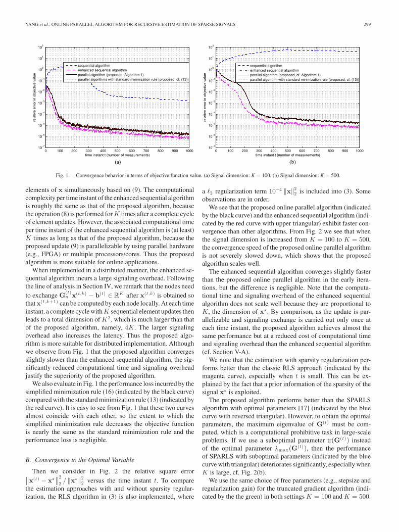
YANG et al.: ONLINE PARALLEL ALGORITHM FOR RECURSIVE ESTIMATION OF SPARSE SIGNALS 299
Fig. 1. Convergence behavior in terms of objective function value. (a) Signal dimension: K = 100. (b) Signal dimension: K = 500.
elements of x simultaneously based on (9). The computationalcomplexity per time instant of the enhanced sequential algorithmis roughly the same as that of the proposed algorithm, becausethe operation (8) is performed for K times after a complete cycleof element updates. However, the associated computational timeper time instant of the enhanced sequential algorithm is (at least)K times as long as that of the proposed algorithm, because theproposed update (9) is parallelizable by using parallel hardware(e.g., FPGA) or multiple processors/cores. Thus the proposedalgorithm is more suitable for online applications.
When implemented in a distributed manner, the enhanced se-quential algorithm incurs a large signaling overhead. Followingthe line of analysis in Section IV, we remark that the nodes needto exchange G(t)
n x(t,k) − b(t) ∈ RK after x(t,k) is obtained sothat x(t,k+1) can be computed by each node locally. At each timeinstant, a complete cycle with K sequential element updates thenleads to a total dimension of K2 , which is much larger than thatof the proposed algorithm, namely, 4K. The larger signalingoverhead also increases the latency. Thus the proposed algo-rithm is more suitable for distributed implementation. Althoughwe observe from Fig. 1 that the proposed algorithm convergesslightly slower than the enhanced sequential algorithm, the sig-nificantly reduced computational time and signaling overheadjustify the superiority of the proposed algorithm.
We also evaluate in Fig. 1 the performance loss incurred by thesimplified minimization rule (16) (indicated by the black curve)compared with the standard minimization rule (13) (indicated bythe red curve). It is easy to see from Fig. 1 that these two curvesalmost coincide with each other, so the extent to which thesimplified minimization rule decreases the objective functionis nearly the same as the standard minimization rule and theperformance loss is negligible.
B. Convergence to the Optimal Variable
Then we consider in Fig. 2 the relative square error∥∥x(t) − x�∥∥2
2 / ‖x�‖22 versus the time instant t. To compare
the estimation approaches with and without sparsity regular-ization, the RLS algorithm in (3) is also implemented, where
a �2 regularization term 10−4 ‖x‖22 is included into (3). Some
observations are in order.We see that the proposed online parallel algorithm (indicated
by the black curve) and the enhanced sequential algorithm (indi-cated by the red curve with upper triangular) exhibit faster con-vergence than other algorithms. From Fig. 2 we see that whenthe signal dimension is increased from K = 100 to K = 500,the convergence speed of the proposed online parallel algorithmis not severely slowed down, which shows that the proposedalgorithm scales well.
The enhanced sequential algorithm converges slightly fasterthan the proposed online parallel algorithm in the early itera-tions, but the difference is negligible. Note that the computa-tional time and signaling overhead of the enhanced sequentialalgorithm does not scale well because they are proportional toK, the dimension of x� . By comparison, as the update is par-allelizable and signaling exchange is carried out only once ateach time instant, the proposed algorithm achieves almost thesame performance but at a reduced cost of computational timeand signaling overhead than the enhanced sequential algorithm(cf. Section V-A).
We note that the estimation with sparsity regularization per-forms better than the classic RLS approach (indicated by themagenta curve), especially when t is small. This can be ex-plained by the fact that a prior information of the sparsity of thesignal x� is exploited.
The proposed algorithm performs better than the SPARLSalgorithm with optimal parameters [17] (indicated by the bluecurve with reversed triangular). However, to obtain the optimalparameters, the maximum eigenvalue of G(t) must be com-puted, which is a computational prohibitive task in large-scaleproblems. If we use a suboptimal parameter tr(G(t)) insteadof the optimal parameter λmax(G(t)), then the performanceof SPARLS with suboptimal parameters (indicated by the bluecurve with triangular) deteriorates significantly, especially whenK is large, cf. Fig. 2(b).
We use the same choice of free parameters (e.g., stepsize andregularization gain) for the truncated gradient algorithm (indi-cated by the the green) in both settings K = 100 and K = 500.

300 IEEE TRANSACTIONS ON SIGNAL AND INFORMATION PROCESSING OVER NETWORKS, VOL. 2, NO. 3, SEPTEMBER 2016
Fig. 2. Relative square error for recursive estimation of time-varying signals. (a) Signal dimension: K = 100. (b) Signal dimension: K = 500.
Fig. 3. Comparison of original signal and estimated signal at different timeinstant: t = 100 in the upper plot and t = 1000 in the lower plot.
It is observed from the comparison of Fig. 2(a) and (b) thatthe truncated gradient algorithm [18] is sensitive to the choiceof free parameters and no general rule applies to all problemparameters. Furthermore, it converges slowly because it is es-sentially a gradient method. By comparison, no pretuning isrequired in the proposed algorithm and simple closed-form ex-pressions exist for each update. The proposed algorithm is easyto use in practice and robust to changes in problem parameters.
The precision of the estimated signal by the proposed on-line parallel algorithm (after 100 and 1000 time instant, respec-tively) is shown element-wise in Fig. 3 when K = 100. Given100 measurements, we observe from the upper plot of Fig. 3that the proposed online parallel algorithm can accurately esti-mate the support of x� , while as expected, the estimated signalbased on the RLS algorithm is not sparse. When the number ofmeasurements is increased to 1000, we can see from the lower
Fig. 4. Weight factor in time- and norm-weighted sparsity regularization.
plot of Fig. 3 that the value of x� is accurately estimated by theproposed online parallel algorithm. The same observation holdsfor the RLS algorithm as well because x(t)
rls → x� .
C. Weight Factor in Time- and Norm-WeightedSparsity Regularization
In Fig. 4 we simulate the weight factor Wμ ( t ) (|x(t)rls,k |) ver-
sus the time instant t in time- and norm-weighted sparsityregularization, where K = 100, k = 1 is used in the upper plotand k = 11 in the lower plot. The parameters are the same as inthe previous simulation examples, except that μ(t) = 1/t0.4 andx� are generated such that the first 0.1 × K elements (where0.1 is the proportion of nonzero elements of x� ) are nonzerowhile all other elements are zero. The weight factors of other el-ements are omitted because they exhibit similar behavior as theones plotted in Fig. 4. As analyzed, Wμ ( t ) (|w(t)
rls,1 |), the weightfactor of the first element, where x�
1 �= 0, quickly converges tozero, while Wμ ( t ) (|w(t)
rls,11 |), the weight factor of the eleventh
YANG et al.: ONLINE PARALLEL ALGORITHM FOR RECURSIVE ESTIMATION OF SPARSE SIGNALS 301
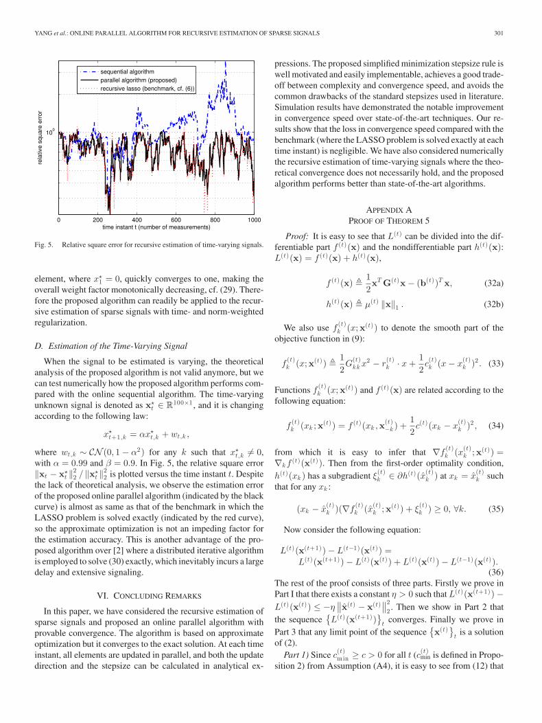
Fig. 5. Relative square error for recursive estimation of time-varying signals.
element, where x�1 = 0, quickly converges to one, making the
overall weight factor monotonically decreasing, cf. (29). There-fore the proposed algorithm can readily be applied to the recur-sive estimation of sparse signals with time- and norm-weightedregularization.
D. Estimation of the Time-Varying Signal
When the signal to be estimated is varying, the theoreticalanalysis of the proposed algorithm is not valid anymore, but wecan test numerically how the proposed algorithm performs com-pared with the online sequential algorithm. The time-varyingunknown signal is denoted as x�
t ∈ R100×1 , and it is changingaccording to the following law:
x�t+1,k = αx�
t,k + wt,k ,
where wt,k ∼ CN (0, 1 − α2) for any k such that x�t,k �= 0,
with α = 0.99 and β = 0.9. In Fig. 5, the relative square error‖xt − x�
t ‖22 / ‖x�
t ‖22 is plotted versus the time instant t. Despite
the lack of theoretical analysis, we observe the estimation errorof the proposed online parallel algorithm (indicated by the blackcurve) is almost as same as that of the benchmark in which theLASSO problem is solved exactly (indicated by the red curve),so the approximate optimization is not an impeding factor forthe estimation accuracy. This is another advantage of the pro-posed algorithm over [2] where a distributed iterative algorithmis employed to solve (30) exactly, which inevitably incurs a largedelay and extensive signaling.
VI. CONCLUDING REMARKS
In this paper, we have considered the recursive estimation ofsparse signals and proposed an online parallel algorithm withprovable convergence. The algorithm is based on approximateoptimization but it converges to the exact solution. At each timeinstant, all elements are updated in parallel, and both the updatedirection and the stepsize can be calculated in analytical ex-
pressions. The proposed simplified minimization stepsize rule iswell motivated and easily implementable, achieves a good trade-off between complexity and convergence speed, and avoids thecommon drawbacks of the standard stepsizes used in literature.Simulation results have demonstrated the notable improvementin convergence speed over state-of-the-art techniques. Our re-sults show that the loss in convergence speed compared with thebenchmark (where the LASSO problem is solved exactly at eachtime instant) is negligible. We have also considered numericallythe recursive estimation of time-varying signals where the theo-retical convergence does not necessarily hold, and the proposedalgorithm performs better than state-of-the-art algorithms.
APPENDIX APROOF OF THEOREM 5
Proof: It is easy to see that L(t) can be divided into the dif-ferentiable part f (t)(x) and the nondifferentiable part h(t)(x):L(t)(x) = f (t)(x) + h(t)(x),
f (t)(x) � 12xT G(t)x − (b(t))T x, (32a)
h(t)(x) � μ(t) ‖x‖1 . (32b)
We also use f(t)k (x;x(t)) to denote the smooth part of the
objective function in (9):
f(t)k (x;x(t)) � 1
2G
(t)kk x2 − r
(t)k · x +
12c(t)k (x − x
(t)k )2 . (33)
Functions f(t)k (x;x(t)) and f (t)(x) are related according to the
following equation:
f(t)k (xk ;x(t)) = f (t)(xk ,x(t)
−k ) +12c(t)(xk − x
(t)k )2 , (34)
from which it is easy to infer that ∇f(t)k (x(t)
k ;x(t)) =∇kf (t)(x(t)). Then from the first-order optimality condition,h(t)(xk ) has a subgradient ξ
(t)k ∈ ∂h(t)(x(t)
k ) at xk = x(t)k such
that for any xk :
(xk − x(t)k )(∇f
(t)k (x(t)
k ;x(t)) + ξ(t)k ) ≥ 0, ∀k. (35)
Now consider the following equation:
L(t)(x(t+1)) − L(t−1)(x(t)) =L(t)(x(t+1)) − L(t)(x(t)) + L(t)(x(t)) − L(t−1)(x(t)).
(36)The rest of the proof consists of three parts. Firstly we prove inPart I that there exists a constant η > 0 such that L(t)(x(t+1)) −L(t)(x(t)) ≤ −η
∥∥x(t) − x(t)∥∥2
2 . Then we show in Part 2 thatthe sequence
{L(t)(x(t+1))
}t
converges. Finally we prove inPart 3 that any limit point of the sequence
{x(t)
}t
is a solutionof (2).
Part 1) Since c(t)min ≥ c > 0 for all t (c(t)
min is defined in Propo-sition 2) from Assumption (A4), it is easy to see from (12) that
302 IEEE TRANSACTIONS ON SIGNAL AND INFORMATION PROCESSING OVER NETWORKS, VOL. 2, NO. 3, SEPTEMBER 2016
the following is true:
L(t)(x(t) + γ(x(t) − x(t))) − L(t)(x(t))
≤ −γ(c − 1
2λmax(G(t))γ
)∥∥x(t) − x(t)∥∥2
2 , 0 ≤ γ ≤ 1.
Since λmax(G(t)) is a continuous function [47] and G(t) con-verges to a positive definite matrix by Assumption (A1’), thereexists a λ < +∞ such that λ ≥ λmax(G(t)) for all t. We thusconclude from the preceding inequality that for all 0 ≤ λ ≤ 1:
L(t)(x(t) + γ(x(t) − x(t))) − L(t)(x(t))
≤ −γ
(c − 1
2λγ
)∥∥x(t) − x(t)∥∥2
2 . (37)
It follows from (15), (16) and (37) that
L(t)(x(t+1))
≤ f (t)(x(t) + γ(t)(x(t) − x(t)))
+ (1 − γ(t))h(t)(x(t)) + γ(t)h(t)(x(t)) (38)
≤ f (t)(x(t) + γ(x(t) − x(t)))
+ (1 − γ)h(t)(x(t)) + γh(t)(x(t)) (39)
≤ L(t)(x(t)) − γ(c − 12λγ)
∥∥x(t) − x(t)∥∥2
2 . (40)
Since the inequalities in (40) are true for any 0 ≤ γ ≤ 1, weset γ = min(c/λ, 1). Then it is possible to show that there is aconstant η > 0 such that
L(t)(x(t+1)) − L(t)(x(t)) ≤ L(t)(x(t+1)) − L(t)(x(t))
≤ −η∥∥x(t) − x(t)
∥∥22 . (41)
Besides this, because of Step 3 in Algorithm 1, x(t+1) is in thefollowing lower level set of L(t)(x):
L(t)≤0 � {x : L(t)(x) ≤ 0}. (42)
Because ‖x‖1 ≥ 0 for any x, (42) is a subset of
{x :
12xT G(t)x − (b(t))T x ≤ 0
},
which is a subset of
L(t)≤0 �
{x :
12λmax(G(t)) ‖x‖2
2 − (b(t))T x ≤ 0}
. (43)
Since G(t) and b(t) converges and limt→∞ G(t) � 0, there ex-ists a bounded set, denoted asL≤0 , such thatL(t)
≤0 ⊆ L(t)≤0 ⊆ L≤0
for all t; thus the sequence {x(t)} is bounded and we denote itsupper bound as x.
Part 2) Combining (36) and (41), we have the following:
L(t+1)(x(t+2)) − L(t)(x(t+1))
≤ L(t+1)(x(t+1)) − L(t)(x(t+1))
= f (t+1)(x(t+1)) − f (t)(x(t+1))
+ h(t+1)(x(t+1)) − h(t)(x(t+1))
≤ f (t+1)(x(t+1)) − f (t)(x(t+1)), (44)
where the last inequality comes from the decreasing property ofμ(t) by Assumption (A3’). Recalling the definition of f (t)(x)in (32), it is easy to see that
(t + 1)(f (t+1)(x(t+1)) − f (t)(x(t+1)))
= l(t+1)(x(t+1)) − 1t
t∑τ =1
l(τ )(x(t+1)),
where
l(t)(x) �N∑
n=1
(y(t)n − (g(t)
n )T x)2 .
Taking the expectation of the preceding equation with respectto {y(t+1)
n ,g(t+1)n }N
n=1 , conditioned on the natural history up totime t + 1, denoted as F (t+1) :
F (t+1) ={x(0) , . . . ,x(t+1) ,
{g(0)
n , . . . ,g(t)n
}n,{y
(0)n , . . . , y
(t)n
}n
},
we have
E[(t + 1)(f (t+1) (x(t+1) ) − f (t) (x(t+1) ))|F (t+1)]
= E[l(t+1) (x(t+1) )|F (t+1)] − 1
t
t∑τ =1
E[l(τ ) (x(t+1) )|F (t+1)]
= E[l(t+1) (x(t+1) )|F (t+1)] − 1
t
t∑τ =1
l(τ ) (x(t+1) ), (45)
where the second equality comes from the observation thatl(τ )(x(t+1)) is deterministic as long as F (t+1) is given. Thistogether with (44) indicates that
E[L(t+1) (x(t+2) ) − L(t) (x(t+1) )|F (t+1)]≤ E
[f (t+1) (x(t+1) ) − f (t) (x(t+1) )|F (t+1)]
≤ 1t + 1
(E[l(t+1) (x(t+1) )|F (t+1)]− 1
t
t∑τ =1
l(τ ) (x(t+1) )
)
≤ 1t + 1
∣∣∣∣∣E [l(t+1) (x(t+1) )|F (t+1)] − 1t
t∑τ =1
l(τ ) (x(t+1) )
∣∣∣∣∣ ,

YANG et al.: ONLINE PARALLEL ALGORITHM FOR RECURSIVE ESTIMATION OF SPARSE SIGNALS 303
and[E[L(t+1)(x(t+2)) − L(t)(x(t+1))|F (t+1)
]]0
≤ 1t + 1
∣∣∣∣∣E[l(t+1)(x(t+1))|F (t+1)
]− 1
t
t∑τ =1
l(τ )(x(t+1))
∣∣∣∣∣≤ 1
t + 1supx∈X
∣∣∣∣∣E[l(t+1)(x)|F (t+1)
]− 1
t
t∑τ =1
l(τ )(x)
∣∣∣∣∣ ,(46)
where [x]0 = max(x, 0), and X in (46) with X � {x(1) ,x(2) , . . . , } is the complete path of x.
Now we derive an upper bound on the expected value of theright hand side of (46):
E
[supx∈X
∣∣∣∣∣E [l(t+1) (x)|F (t+1)] − 1t
t∑τ =1
l(τ ) (x)
∣∣∣∣∣]
= E
[supx∈X
∣∣y(t) − (r(t)2 )T x + xT R(t)
3 x∣∣]
≤ E
[supx∈X
∣∣y(t)∣∣+ sup
x∈X
∣∣(b(t) )T x∣∣+ sup
x∈X
∣∣xT G(t)x∣∣]
= E
[supx∈X
∣∣y(t)∣∣]+E
[supx∈X
∣∣(b(t) )T x∣∣]+E
[supx∈X
∣∣xT G(t)x∣∣],(47)
where
y(t) � 1t
t∑τ =1
N∑n=1
(Eyn
[y2
n
]− (y(τ )
n )2)
,
b(t) � 1t
t∑τ =1
N∑n=1
2(E{yn ,gn } [yngn ] − y(τ )
n g(τ )n
),
G(t) � 1t
t∑τ =1
N∑n=1
(Egn
[gngn ] − g(t)n g(τ )T
n
).
Then we bound each term in (47) individually. For the first term,since y(t) is independent of x(t) ,
E
[supx∈X
∣∣y(t)∣∣] = E
[∣∣y(t)∣∣] = E
[√(y(t))2
]
≤√
E[(y(t))2
]≤√
σ21
t(48)
for some σ1 < ∞, where the second equality comes fromJensen’s inequality. Because of Assumptions (A1’) and (A2),y(t) has bounded moments and the existence of σ1 is then justi-fied by the central limit theorem [48].
For the second term of (47), we have
E
[sup
x
∣∣(b(t) )T x∣∣] ≤E
[sup
x(∣∣b(t)
∣∣)T |x|]≤(E[∣∣b(t)
∣∣])T
|x| .
Similar to the line of analysis of (48), there exists a σ2 < ∞such that
E
[supx
∣∣(b(t))T x∣∣] ≤ (
E[∣∣b(t)
∣∣])T
|x| ≤√
σ22
t. (49)
For the third term of (47), we have
E
[supx∈X
∣∣xT G(t)x∣∣]
= E
[max
1≤k≤K
∣∣λk (G(t))∣∣ · ‖x‖2
2
]
= ‖x‖22 · E
[√max{λ2
max(G(t)), λ2min(G(t))}
]
≤ ‖x‖22 ·√E[max{λ2
max(G(t)), λ2min(G(t))}
]
≤ ‖x‖22 ·
√√√√E
[K∑
k=1
λ2k (G(t))
]
= ‖x‖22 ·√E[tr(G(t)(G(t))T
)]≤√
σ23
t(50)
for some σ3 < ∞, where the first equality comes from the obser-vation that x should align with the eigenvector associated withthe eigenvalue with largest absolute value. Then combing (48)–(50), we can claim that there exists σ �
√σ2
1 +√
σ22 +
√σ2
3 >0 such that
E
[supx∈X
∣∣∣∣∣E[l(t+1)(x)|F (t+1)
]− 1
t
t∑τ =1
l(τ )(x)
∣∣∣∣∣]≤ σ√
t.
In view of (46), we have
E[[E[L(t+1)(x(t+2)) − L(t)(x(t+1))|F (t+1)
]]0
]≤ σ
t3/2 .
(51)Summing (51) over t, we obtain
∞∑t=1
E[[E[L(t+1)(x(t+2)) − L(t)(x(t+1))|F (t+1)
]]0
]< ∞.
Then it follows from the quasi-martingale convergence theorem(cf. [42, Th. 6]) that
{L(t)(x(t+1))
}converges almost surely.
Part 3) Combining (36) and (41), we have
L(t)(x(t+1)) − L(t−1)(x(t)) ≤
−η∥∥x(t) − x(t)
∥∥22 + L(t)(x(t)) − L(t−1)(x(t)). (52)
Besides this, it follows from the convergence of{L(t)(x(t+1))
}t
limt→∞
L(t)(x(t+1)) − L(t−1)(x(t)) = 0,
and the strong law of large numbers that
limt→∞
L(t)(x(t)) − L(t−1)(x(t)) = 0.
304 IEEE TRANSACTIONS ON SIGNAL AND INFORMATION PROCESSING OVER NETWORKS, VOL. 2, NO. 3, SEPTEMBER 2016
Taking the limit inferior of both sides of (52), we have
0 = lim inft→∞
{L(t)(x(t+1)) − L(t−1)(x(t))
}≤ lim inf
t→∞
{−η∥∥x(t) − x(t)
∥∥22 + L(t)(x(t)) − L(t−1)(x(t))
}≤ lim inf
t→∞
{−η∥∥x(t) − x(t)
∥∥22
}+ lim sup
t→∞
{L(t)(x(t)) − L(t−1)(x(t))
}= − η · lim sup
t→∞
∥∥x(t) − x(t)∥∥2
2 ≤ 0,
so we can infer that lim supt→∞∥∥x(t) − x(t)
∥∥2 = 0. Since 0 ≤
lim inf t→∞∥∥x(t) − x(t)
∥∥2 ≤ lim supt→∞
∥∥x(t) − x(t)∥∥
2 = 0,we can infer that lim inf t→∞
∥∥x(t) − x(t)∥∥ = 0 and thus
limt→∞∥∥x(t) − x(t)
∥∥ = 0.Consider any limit point of the sequence
{x(t)
}t, denoted as
x(∞) . Since x is a continuous function of x in view of (9) andlimt→∞
∥∥x(t) − x(t)∥∥
2 = 0, it must be limt→∞ x(t) = x(∞) =x(∞) , and the minimum principle in (35) can be simplified as
(xk − x(∞)k )(∇k f (∞)(x(∞)) + ξ
(∞)k ) ≥ 0, ∀xk ,
whose summation over k = 1, . . . ,K leads to
(x − x(∞))T (∇f (∞)(x(∞)) + ξ(∞)) ≥ 0, ∀x.
Therefore x(∞) minimizes L(∞)(x) and x(∞) = x� almostsurely by Lemma 1. Since x� is unique in view of Assump-tions (A1’), the whole sequence {x(t)} has a unique limit pointand it thus converges to x� . The proof is thus completed. �
ACKNOWLEDGMENT
The authors would like to thank the reviewers whose com-ments have greatly improved the quality of the paper.
REFERENCES
[1] Y. Yang, M. Zhang, M. Pesavento, and D. P. Palomar, “An online parallelalgorithm for spectrum sensing in cognitive radio networks,” in Proc. 48thAsilomar Conf. Signals, Syst. Comput., 2014, pp. 1801–1805.
[2] S. Barbarossa, S. Sardellitti, and P. Di Lorenzo, “Distributed detectionand estimation in wireless sensor networks,” in Academic Press Libraryin Signal Processing, R. Chellappa and S. Theodoridis, Eds. New York,NY, USA: Academic, 2014, vol. 2, pp. 329–408.
[3] S. Haykin, “Cognitive radio: Brain-empowered wireless communica-tions,” IEEE J. Sel. Areas Commun., vol. 23, no. 2, pp. 201–220,Feb. 2005.
[4] J. Mitola and G. Maguire, “Cognitive radio: Making software radios morepersonal,” IEEE Pers. Commun., vol. 6, no. 4, pp. 13–18, Aug. 1999.
[5] R. Zhang, Y.-C. Liang, and S. Cui, “Dynamic resource allocation incognitive radio networks,” IEEE Signal Process. Mag., vol. 27, no. 3,pp. 102–114, May 2010.
[6] Y. Yang, G. Scutari, P. Song, and D. P. Palomar, “Robust MIMO cognitiveradio systems under interference temperature constraints,” IEEE J. Sel.Areas Commun., vol. 31, no. 11, pp. 2465–2482, Nov. 2013.
[7] S. Haykin, D. Thomson, and J. Reed, “Spectrum sensing for cognitiveradio,” Proc. IEEE, vol. 97, no. 5, pp. 849–877, May 2009.
[8] S.-J. Kim, E. Dall’Anese, and G. B. Giannakis, “Cooperative spectrumsensing for cognitive radios using Kriged Kalman filtering,” IEEE J. Sel.Topics Signal Process., vol. 5, no. 1, pp. 24–36, Feb. 2011.
[9] F. Zeng, C. Li, and Z. Tian, “Distributed compressive spectrum sensingin cooperative multihop cognitive networks,” IEEE J. Sel. Topics SignalProcess., vol. 5, no. 1, pp. 37–48, Feb. 2011.
[10] O. Mehanna and N. D. Sidiropoulos, “Frugal sensing: Wideband powerspectrum sensing from few bits,” IEEE Trans. Signal Process., vol. 61,no. 10, pp. 2693–2703, May 2013.
[11] S. M. Kay, Fundamentals of Statistical Signal Processing, Volume I:Estimation Theory. Englewood Cliffs, NJ, USA: Prentice-Hall, 1993.
[12] A. Sayed, Adaptive Filters. Hoboken, NJ, USA: Wiley-Interscience, 2008.[13] G. Mateos, I. Schizas, and G. Giannakis, “Distributed recursive least-
squares for consensus-based in-network adaptive estimation,” IEEE Trans.Signal Process., vol. 57, no. 11, pp. 4583–4588, Nov. 2009.
[14] G. Mateos and G. B. Giannakis, “Distributed recursive least-squares: Sta-bility and performance analysis,” IEEE Trans. Signal Process., vol. 60,no. 7, pp. 3740–3754, Jul. 2012.
[15] D. Angelosante, J. A. Bazerque, and G. B. Giannakis, “Online adaptiveestimation of sparse signals: Where RLS meets the �1 -norm,” IEEE Trans.Signal Process., vol. 58, no. 7, pp. 3436–3447, Jul. 2010.
[16] Y. Kopsinis, K. Slavakis, and S. Theodoridis, “Online sparse system iden-tification and signal reconstruction using projections onto weighted �1balls,” IEEE Trans. Signal Process., vol. 59, no. 3, pp. 936–952, Mar.2011.
[17] B. Babadi, N. Kalouptsidis, and V. Tarokh, “SPARLS: The sparse RLSalgorithm,” IEEE Trans. Signal Process., vol. 58, no. 8, pp. 4013–4025,Aug. 2010.
[18] J. Langford, L. Li, and T. Zhang, “Sparse online learning via truncatedgradient,” J. Mach. Learn. Res., vol. 10, pp. 777–801, 2009.
[19] Y. Chen and A. O. Hero, “Recursive �1 ,∞ group Lasso,” IEEE Trans.Signal Process., vol. 60, no. 8, pp. 3978–3987, Aug. 2012.
[20] R. Tibshirani, “Regression shrinkage and selection via the lasso: A ret-rospective,” J. Roy. Statist. Soc. B, Statist. Methodol., vol. 58, no. 1,pp. 267–288, Jun. 1996.
[21] M. A. T. Figueiredo, R. D. Nowak, and S. J. Wright, “Gradient projectionfor sparse reconstruction: Application to compressed sensing and otherinverse problems,” IEEE J. Sel. Topics Signal Process., vol. 1, no. 4,pp. 586–597, Dec. 2007.
[22] S.-J. Kim, K. Koh, M. Lustig, S. Boyd, and D. Gorinevsky, “An interior-point method for large-scale l1 -regularized least squares,” IEEE J. Sel.Topics Signal Process., vol. 1, no. 4, pp. 606–617, Dec. 2007.
[23] A. Beck and M. Teboulle, “A fast iterative shrinkage-thresholding al-gorithm for linear inverse problems,” SIAM J. Imag. Sci., vol. 2, no. 1,pp. 183–202, Jan. 2009.
[24] T. Goldstein and S. Osher, “The split Bregman method for L1-regularizedproblems,” SIAM J. Imag. Sci., vol. 2, no. 2, pp. 323–343, 2009.
[25] F. Facchinei, G. Scutari, and S. Sagratella, “Parallel selective algorithmsfor nonconvex big data optimization,” IEEE Trans. Signal Process.,vol. 63, no. 7, pp. 1874–1889, Nov. 2015.
[26] G. Mateos, J. A. Bazerque, and G. B. Giannakis, “Distributed sparse linearregression,” IEEE Trans. Signal Process., vol. 58, no. 10, pp. 5262–5276,Oct. 2010.
[27] D. P. Bertsekas and J. N. Tsitsiklis, Parallel and Distributed Computation:Numerical Methods. Englewood Cliffs, NJ, USA: Prentice-Hall, 1989.
[28] S. Chouvardas, K. Slavakis, Y. Kopsinis, and S. Theodoridis, “A sparsitypromoting adaptive algorithm for distributed learning,” IEEE Trans. SignalProcess., vol. 60, no. 10, pp. 5412–5425, Oct. 2012.
[29] P. Di Lorenzo and A. H. Sayed, “Sparse distributed learning basedon diffusion adaptation,” IEEE Trans. Signal Process., vol. 61, no. 6,pp. 1419–1433, Mar. 2013.
[30] P. Di Lorenzo, “Diffusion adaptation strategies for distributed estima-tion over Gaussian Markov random fields,” IEEE Trans. Signal Process.,vol. 62, no. 21, pp. 5748–5760, Nov. 2014.
[31] Y. Chen, Y. Gu, and A. O. Hero, “Sparse LMS for system identification,”in Proc. IEEE Int. Conf. Acoust., Speech, Signal Process., no. 3, pp. 3125–3128, 2009.
[32] Y. Chen, Y. Gu, and A. O. Hero, “Regularized least-mean-square algorithms,” Tech. Rep., Jun. 2010. [Online]. Available:http://arxiv.org/abs/1012.5066
[33] Y. Liu, C. Li, and Z. Zhang, “Diffusion sparse least-mean squares overnetworks,” IEEE Trans. Signal Process., vol. 60, no. 8, pp. 4480–4485,Aug. 2012.
[34] Y. Yang, G. Scutari, D. P. Palomar, and M. Pesavento, “A parallel de-composition method for nonconvex stochastic multi-agent optimizationproblems,” IEEE Trans. Signal Process.,vol. 64, no. 11, pp. 2949–2964,Jun. 2016.
[35] G. Scutari, F. Facchinei, P. Song, D. P. Palomar, and J.-S. Pang, “De-composition by partial linearization: Parallel optimization of multi-agentsystems,” IEEE Trans. Signal Process., vol. 62, no. 3, pp. 641–656,Feb. 2014.
[36] Z. Quan, S. Cui, H. Poor, and A. Sayed, “Collaborative wideband sensingfor cognitive radios,” IEEE Signal Process. Mag., vol. 25, no. 6, pp. 60–73,Nov. 2008.
[37] S. Ghadimi and G. Lan, “Optimal stochastic approximation algorithmsfor strongly convex stochastic composite optimization I: A generic

YANG et al.: ONLINE PARALLEL ALGORITHM FOR RECURSIVE ESTIMATION OF SPARSE SIGNALS 305
algorithmic framework,” SIAM J. Optimization, vol. 22, no. 4, pp. 1469–1492, Nov. 2012.
[38] S. Boyd, N. Parikh, E. Chu, B. Peleato, and J. Eckstein, “Distributedoptimization and statistical learning via the alternating direction methodof multipliers,” Found. Trends Mach. Learn., vol. 3, no. 1, pp. 1–122,2011.
[39] D. P. Bertsekas, Nonlinear Programming. Belmont, MA, USA: AthenaScientific, 1999.
[40] S. Boyd and L. Vandenberghe, Convex Optimization. Cambridge, U.K.:Cambridge Univ. Press, 2004.
[41] J. F. Sturm, “Using SeDuMi 1.02: A Matlab toolbox for optimizationover symmetric cones,” Optimization Methods Softw., vol. 11, no. 1–4,pp. 625–653, Jan. 1999.
[42] J. Mairal, F. Bach, J. Ponce, and G. Sapiro, “Online learning for ma-trix factorization and sparse coding,” J. Mach. Learning Res., vol. 11,pp. 19–60, 2010.
[43] M. Razaviyayn, M. Sanjabi, and Z.-Q. Luo, “A stochastic successive min-imization method for nonsmooth nonconvex optimization,” Math. Pro-gram., Jun. 2013. [Online]. Available: http://arxiv.org/abs/1307.4457
[44] S. Sundaram and C. Hadjicostis, “Distributed function calculation andconsensus using linear iterative strategies,” IEEE J. Sel. Areas Commun.,vol. 26, no. 4, pp. 650–660, May 2008.
[45] W. H. Greene, Econometric Analysis, 7th ed. Englewood Cliffs, NJ, USA:Prentice-Hall, 2011.
[46] MOSEK, “The MOSEK Optimization Toolbox for MATLAB Manual,Version 7.0.” 2013. [Online]. Available: https://www.mosek.com/
[47] R. A. Horn and C. R. Johnson, Matrix Analysis. Cambridge, U.K.: Cam-bridge Univ. Press, 1985.
[48] R. Durrett, Probability: Theory and Examples, 4th ed. Cambridge, U.K.:Cambridge Univ. Press, 2010.
Yang Yang (S’09–M’13) received the B.S. degreefrom the School of Information Science and En-gineering, Southeast University, Nanjing, China, in2009, and the Ph.D. degree from the Departmentof Electronic and Computer Engineering, The HongKong University of Science and Technology, HongKong. From November 2013 to November 2015, hehad been a Postdoctoral Research Associate at theCommunication Systems Group, Darmstadt Univer-sity of Technology, Darmstadt, Germany. He joinedIntel Deutschland GmbH as a Research Scientist in
December 2015.His research interests include distributed solution methods in convex opti-
mization, nonlinear programming, and game theory, with applications in com-munication networks, signal processing, and financial engineering.
Marius Pesavento (M’00) received the Dipl.-Ing. and M.Eng. degrees from Ruhr-UniversitatBochum, Bochum, Germany, and McMaster Uni-versity, Hamilton, ON, Canada, in 1999 and 2000,respectively, and the Dr.-Ing. degree in electrical en-gineering from Ruhr-Universitat Bochum in 2005.Between 2005 and 2007, he was a Research Engineerat FAG Industrial Services GmbH, Aachen, Germany.From 2007 to 2009, he was the Director of the Sig-nal Processing Section at MIMOon GmbH, Duisburg,Germany. In 2010, he became an Assistant Professor
for Robust Signal Processing and a Full Professor for Communication Systemsin 2013, Department of Electrical Engineering and Information Technology,Darmstadt University of Technology, Darmstadt, Germany. His research inter-ests include robust signal processing and adaptive beamforming, high-resolutionsensor array processing, multiantenna and multiuser communication systems,distributed, sparse, and mixed-integer optimization techniques for signal pro-cessing and communications, statistical signal processing, spectral analysis, andparameter estimation. He has received the 2003 ITG/VDE Best Paper Award, the2005 Young Author Best Paper Award of the IEEE TRANSACTIONS ON SIGNAL
PROCESSING, and the 2010 Best Paper Award of the CROWNCOM conference.He is a Member of the Editorial board of the EURASIP Signal Processing Jour-nal, an Associate Editor for the IEEE TRANSACTIONS ON SIGNAL PROCESSING.He is currently serving the second term as a Member of the Sensor Array andMultichannel Technical Committee of the IEEE Signal Processing Society.
Mengyi Zhang (S’09–M’13) received the B.Sc. de-gree from the Department of Electronic Information,Huazhong University of Science and Technology,Wuhan, China, in 2009, and the Ph.D. degree fromthe Department of Electronic and Computer Engi-neering, The Hong Kong University of Science andEngineering, Hong Kong, in 2013. She is currently aPostdoctoral Research Associate in the Departmentof Computer Science and Engineering, The ChineseUniversity of Hong Kong, Hong Kong. Her researchinterests include statistical signal processing, opti-
mization, and machine learning with applications in wireless communicationsand financial systems.
Daniel P. Palomar (S’99–M’03–SM’08–F’12) re-ceived the Electrical Engineering and Ph.D. degreesfrom the Technical University of Catalonia (UPC),Barcelona, Spain, in 1998 and 2003, respectively.
He is a Professor in the Department of Electronicand Computer Engineering, Hong Kong Universityof Science and Technology (HKUST), Hong Kongwhich he joined in 2006. Since 2013, he is a Fellowof the Institute for Advance Study at HKUST. Hehad previously held several research appointments,namely, at King’s College London, London, U.K.;
Stanford University, Stanford, CA, USA; Telecommunications TechnologicalCenter of Catalonia, Barcelona, Spain; Royal Institute of Technology, Stock-holm, Sweden; University of Rome “La Sapienza,” Rome, Italy; and PrincetonUniversity, Princeton, NJ, USA. His current research interests include appli-cations of convex optimization theory, game theory, and variational inequalitytheory to financial systems, big data systems, and communication systems.
He has received the 2004/06 Fulbright Research Fellowship, the 2004 and2015 (coauthor) Young Author Best Paper Awards by the IEEE Signal Pro-cessing Society, the 2002/03 best Ph.D. prize in Information Technologies andCommunications by the UPC, the 2002/03 Rosina Ribalta first prize for the BestDoctoral Thesis in information technologies and communications by the EpsonFoundation, and the 2004 prize for the best Doctoral Thesis in advanced mobilecommunications by the Vodafone Foundation.
He is a Guest Editor of the IEEE JOURNAL OF SELECTED TOPICS IN SIGNAL
PROCESSING2016 Special Issue on “Financial Signal Processing and MachineLearning for Electronic Trading” and has been an Associate Editor of IEEETRANSACTIONS ON INFORMATION THEORY and of IEEE TRANSACTIONS ON
SIGNAL PROCESSING, a Guest Editor of the IEEE SIGNAL PROCESSING MAGA-ZINE 2010 Special Issue on “Convex Optimization for Signal Processing,” theIEEE JOURNAL ON SELECTED AREAS IN COMMUNICATIONS 2008 Special Issueon “Game Theory in Communication Systems,” and the IEEE JOURNAL ON
SELECTED AREAS IN COMMUNICATIONS 2007 Special Issue on “Optimizationof MIMO Transceivers for Realistic Communication Networks.”