
28&7 A,- f’ for the Period Aug. 15, 1987 · Sixth Month Process Report for the Period Aug. 15,...
62
-c i d /28&7 A,- f’ Sixth Month Projess Report for the Period Aug. 15, 1987 - Feb. 14, 1988 on Computer-Aided Modeling and Prediction of Performance of the Modified Lundell Class of Alternators in Space Station Solar Dynamic Power Systems (r Grant No. NAG3 - 818 by Nabeel A. 0. Demerdash Principal Investigator and Ren-hong Wang Research Assistant L 5 Clarkson University rn Department of Electrical and Computer Engineering Potsdam, New York, March 15, 1988 (YASA-CR-Y82S38) COMEGIER-AICLE RODEZllliG 188-19000 AVD POEDICTfGO OF PEBFCfilAbCE Ck ZCHE IICDIPIED LURDELL CLASS CP ALlBEYATOES IY SEACB STATION SCLAG DYBABXC FCVEL SPSTEES Unclas Semiannual Prcgress iia~ort, 15 Aug. 1987 - G3/44 0120067 Submitted to Solar Dynamic Module Division Mail Stop 500 - 316 NASA Lewis Research Center 21000 Brookpark Road Cleveland, Ohio 44135 https://ntrs.nasa.gov/search.jsp?R=19880009616 2018-07-28T08:48:35+00:00Z
Transcript of 28&7 A,- f’ for the Period Aug. 15, 1987 · Sixth Month Process Report for the Period Aug. 15,...
- c i
d
/28&7 A,- f ’
Sixth Month Projess Report for the Period Aug. 15, 1987 - Feb. 14, 1988
on
Computer-Aided Modeling and Prediction of Performance of the
Modified Lundell Class of Alternators in Space Station
Solar Dynamic Power Systems (r
Grant No. NAG3 - 818
by Nabeel A. 0. Demerdash
Principal Investigator
and
Ren-hong Wang
Research Assistant L
5
Clarkson University rn
Department of Electrical and Computer Engineering
Potsdam, New York, March 15, 1988
(YASA-CR-Y82S38) COMEGIER-AICLE RODEZl l l iG 188-19000 A V D POEDICTfGO OF PEBFCfi lAbCE Ck ZCHE I I C D I P I E D LURDELL CLASS CP ALlBEYATOES IIY SEACB STATION SCLAG D Y B A B X C FCVEL SPSTEES Unclas Semiannual Prcgress i ia~ort , 15 Aug. 1987 - G3/44 0120067
Submitted to
Solar Dynamic Module Division
Mail Stop 500 - 316
NASA Lewis Research Center
21000 Brookpark Road
Cleveland, Ohio 44135
https://ntrs.nasa.gov/search.jsp?R=19880009616 2018-07-28T08:48:35+00:00Z
Sixth Month Process Report for the Period Aug. 15, 1987 - Feb. 14, 1988
on
Computer-Aided ModeIing and Prediction of Performance of the
Modified Lundell Class of Alternators in Space Station
Solar Dynamic Power Systems
by
Nabeel A. 0. Demerdash
Principal Investigator
and
Ren-hong Wang
Research Assistant
Department of Electrical and Computer Engineering
C larkson University
Potsdam, New York, March 15, 1988

c
TABLE OF CONTENTS
1.0 Introduction
2.0 Nature of the Geometry of the Modified Lundell Class of
Alternators
3.0 Basic Building Blocks and Nature of the Finite Element Grids
3.1 Tetrahedral Finite Elements
3.2 Triangular Prism Super-Elements
3.3 Filling Technique
4.0 Stator Finite Element Grid Geometry
4.1 Basic Grid Module for the Stator Grid
4.2 Stator Grid Presentat ion
4.3 Programming Considerations
5.0 Rotor Finite Element Grid Geometry
8.0 Immediate Forthcoming Efforts
7.0 Conclusions
8.0 References
t
1.0 INTRODUCTION
The main purpose of this project is the development of computer-aided models
for purposes of studying the effects of various design changes on the parameters and
performance characteristics of the Modified Lundell Class of Alternators (MLA),
as components of a solar dynamic power system supplying electric energy needs in
the forthcoming space station. Hence, this computer-aided modeling effort is ex-
pected to yield the tools necessary to assesses advantages and drawbacks of various
proposed design variations (including material, geometric, and winding changes)
on the basic design concept of the MLA class of alternators. This effort is expected
to include the steady state as well as the dynamic performance characteristics of
these types of high speed machines.
Key to this modeling effort is the computation of magnetic field distribution
in this class of MLAs. Knowledge of such magnetic field distribution is the key
element in finding the following: fluxes, induced emfs in various windings, wind-
ing inductances (reactances), various time constants and damping effects, critical
effects of saturation on performance, critical areas of high magnetic and electric
loading in various parts of such machines, amd hence loss distributions, efficiencies,
dynamic characteristics and parameters, etc..
The nature of the magnetic field in this class of machines is unfortunately
three-dimensional (3-D) , and does not lend itself to reasonable two-dimensional
(2-D) approximations. Accordingly, the magnetic field computation effort will en-
tirely be based on the 3-D finite element (FE) method. In this method, one must
discretize the solution volume, or region of interest, into small subdivisions called
finite elements. The basic 3-D shaped discretization volume or element which will
1

L
L
be used in this investigation is the tetrahedron. The tetrahedral shape is the sim-
plist, most general, and most flexible to use in a discretization process. Also, its
finite element algebra is the most simple to develop. Hence, it possesses several
attractive features from a numerical or computational standpoint. However, inter-
mediate super-elements, such as triangular prisms and/or hexahedrons are resorted
to in the development of the necessary finite element grids, for easier implementa-
tion and mental visualization of 3-D objects and parts.
Accordingly, in the earIy tasks of this investigation stator and rotor finite
element grid discretizations for this class of MLAs are being developed. This effort
was devided into stator and rotor grid discretizations, for purposes of being able to
study the magnetic field distribution at various relative rotor to stator positions,
as required by any rotating machinery modeling and analysis effort.
In this report, details of the development of the stator 3-D finite element grid
are given. Also, a preliminary look at the early stage of 3-D FE rotor grid devel-
opment effort is presented. In addition, a review of the immediately forthcoming
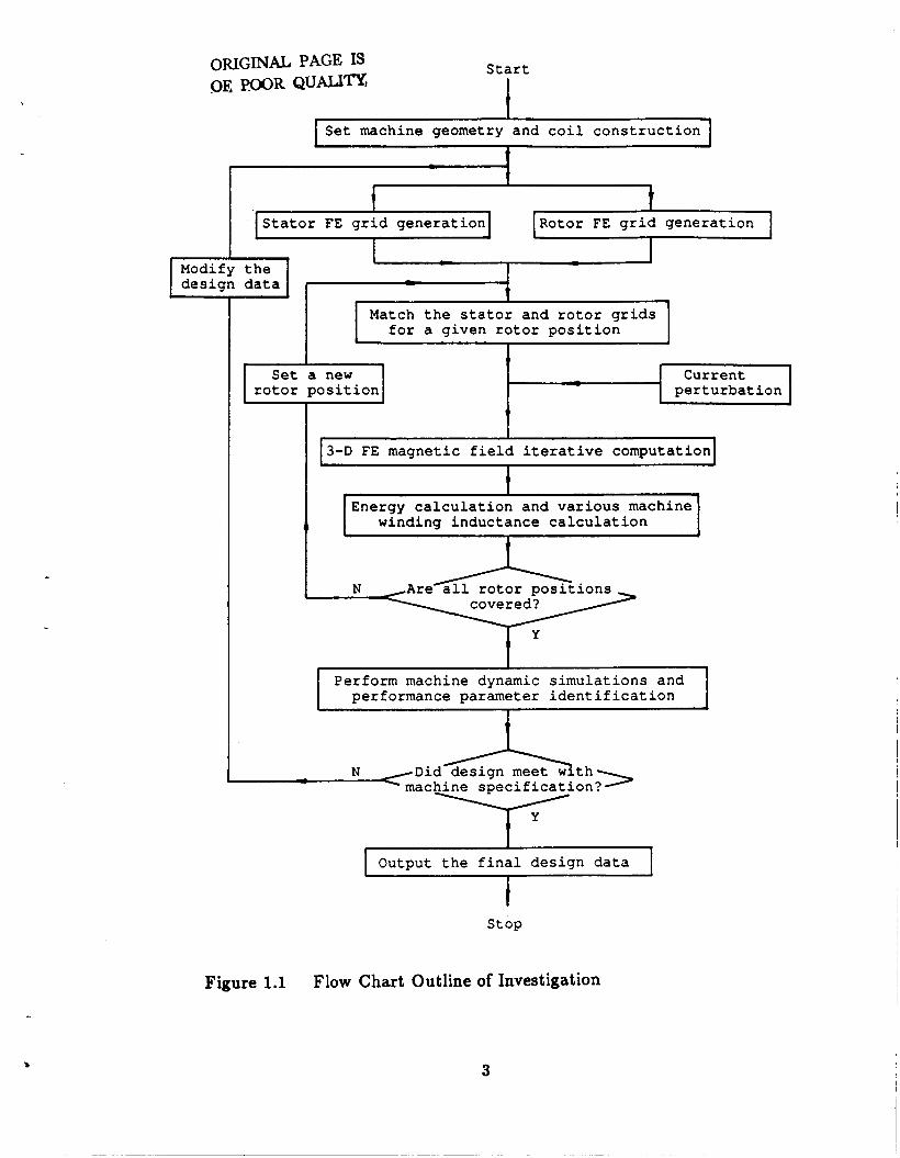
tasks [I], based on the task flow chart, Figure 1.1, are discussed in the later portions
of this report.
2
ORIGINAL PAGE IS OE P W R QUAJJm,
~ ~ ~ ~~
Perform machine dynamic s i m u l a t i o n s and per formance parameter i d e n t i f i c a t i o n
S t a r t
I I I S e t machine geometry and c o i l c o n s t r u c t i o n
I 1
S t a t o r FE g r i d g e n e r a t i o n Rotor FE g r id g e n e r a t i o n
Match t h e s t a t o r and r o t o r g r ids f o r a g i v e n r o t o r p o s i t i o n
S e t a new t
I C u r r e n t p e r t u r b a t i o n
I I J
t
winding i n d u c t a n c e c a l c u l a t i o n
I '
t
1
Output t h e f i n a l d e s i g n data
1 s t o p
Figure 1.1 Flow Chart Outline of Investigation
3
2.0 NATURE OF THE GEOMETRY OF THE MODIFIED
LUNDELL CLASS OF ALTERNATORS
The base example chosen for the current stage of this investigation is a 14.3
kVA, 1200 Hz Modified Lundell Alternator. This machine was developed for NASA
Lewis Research Center for purposes of space power systems. The development of
this machine by the AiResearch Manufacturing Company took place, in the 1960s.
A very high rated speed, 36000 rpm, is the design key for the machine to re-
duce its volume and weight per voltampere to meet with the volume and weight
limitation requirements in space applications. In this alternator, both the field
excitation winding and the armature winding are stationary, and a mechanically
strong, smooth rotor with special configuration is supported by gas bearings. The
particular constructional feature of this MLA type of machine causes a different
three dimensional pattern of magnetic flux paths inside the alternator, as compared
with the predominantly two dimensional pattern of flux in ordinary synchronous
machines. Accordinly, to calculate various winding inductances and performance
parameters of this machine from magnetic field solutions, three dimensional mag-
netic field computations must be carried out through the machine geometry.
The basic configuration of this 14.3 kVA MLA with each major electric com-
ponent identified, is illustrated in Figure 2.1, copied from Reference [2]. The stator
contains a conventional three phase armature, as well as stationary field coils, which
create the main magnetic flux in the axial direction of the machine. The rotor con-
sists of two identical magnetic sections, as shown in Figure 2.2, also copied from
Referenc [2]. Inserted between these two magnetic sections is a nonmagnetic sepa-
rator. The rotor establishes four rotating magnetic poles when it carries magnetic
i 4

etic
Figure 2.1 Cutaway View of the Modified Lundell Alternator
-- . -- ------- \ \
Nonmagnetic ,/
section --'
Figure 2.2 Rotor of Example 14.3 kVA MLA
5

flux and rotates. Also, the rotor carries portions of the axial paths which contribute
to the overall values of the various machine winding inductances.
In Figure 2.1, the arrows are used to show the main magnetic flux path in the
MLA machine. The flux starts from a north pole on the rotor, crosses the main
airgap and proceeds radially through the stator teeth into the laminated stator
core. It then goes circumferentially through the stator core for a distance of one
pole pitch, enters the teeth radially and crosses the main airgap, in an opposite
direction to the previous crossing, into the adjacent south poles on the rotor. The
flux then goes axially down the rotor and crosses the first auxiliary air gap into
the endbell and the outer frame. It leaves the other end of the frame , crosses
the second auxiliary air gap, and completes its path back to the north pole from
which it started. Such a picture of magnetic flux shows that the magnetic field in-
side the machine has not only radial and circumferential components in the stator
laminations but also axial component in the rotor and the housing parts. There-
fore, the magnetic field of the MLA machine has a true three dimensional nature.
Accordingly, these investigators hold the view that no practical two dimensional
approximation can be made to model such a magnetic field distribution, with a
reasonably assured accuracy of results.
Accordingly, a three dimensional finite element vector potential solution model
will be developed for the magnetic field calculation. As a first step in performing
finite element calculations, three dimensional finite element grids which discretize
the machine geometry into finite small sub-regions are generated. Detailed work of
the generation of the finite element grids will be presented in Sections 3.0 through
5.0 of this report. It should be mentioned that the grid pictures shown later in
this report are only for the example 14.3 kVA MLA machine. The computer pro-
6
I
gram developed for the grid generation has a capability to accommodate different
machine design data and parameters for other cases, with variations in these pa-
rameters such as the key dimensions of the geometry, the number of poles, the
armature coil pitch, the number of turns in various coils, coil dimensions, etc.,
within a practical range.
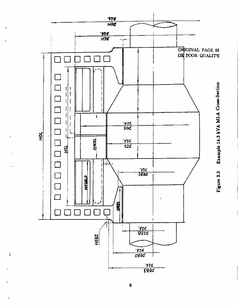
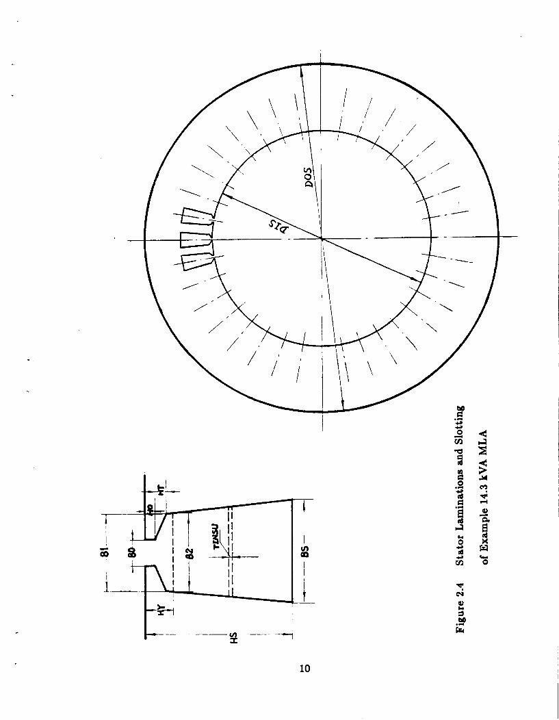
The key geometric dimensions of the cores, windings, etc., of the example ma-
chine are give in Table 2.1, and Figures 2.3 through 2.5. Such a machine geometry
model is utilized here as the solution region for the three dimensional finite element
calculations. The data in Table 2.1 with their corresponding definitions shown in
Figures 2.3 through 2.5, are the input data for the computer algorithm which de-
termines the topology of the finite element grid. As is shown by these figures, this
machine geometry model closely duplicates the physical details of this MLA type of
machine. Thus using this machine geometry model, magnetic field solutions can be
expected to be close to the real magnetic field distribution of the actual machine.
It should be pointed out that a slight approximation was made in developing
the machine geometry model presented above. Namely, that approximation is the
fact that the model has not included ventilation tunnels inside the endbell and the
frame of the machine. Meanwile, the axial thickness of the endbell and the outside
diameter of the frame are modified to compensate for the geometry change due
to this exclusion. Since the degree of magnetic saturation in the housing parts is
usually a moderate one, such an approximation, if implemented carefully, will not
affect the total magnetic energy calculation of the machine. This means that the
accuracy of the various inductances calculated from energy perturbation, as well as
other machine parameters, will not be affected. The purpose of this approximation
is to reduce the number of the elements for the discretization of the housing part,
7
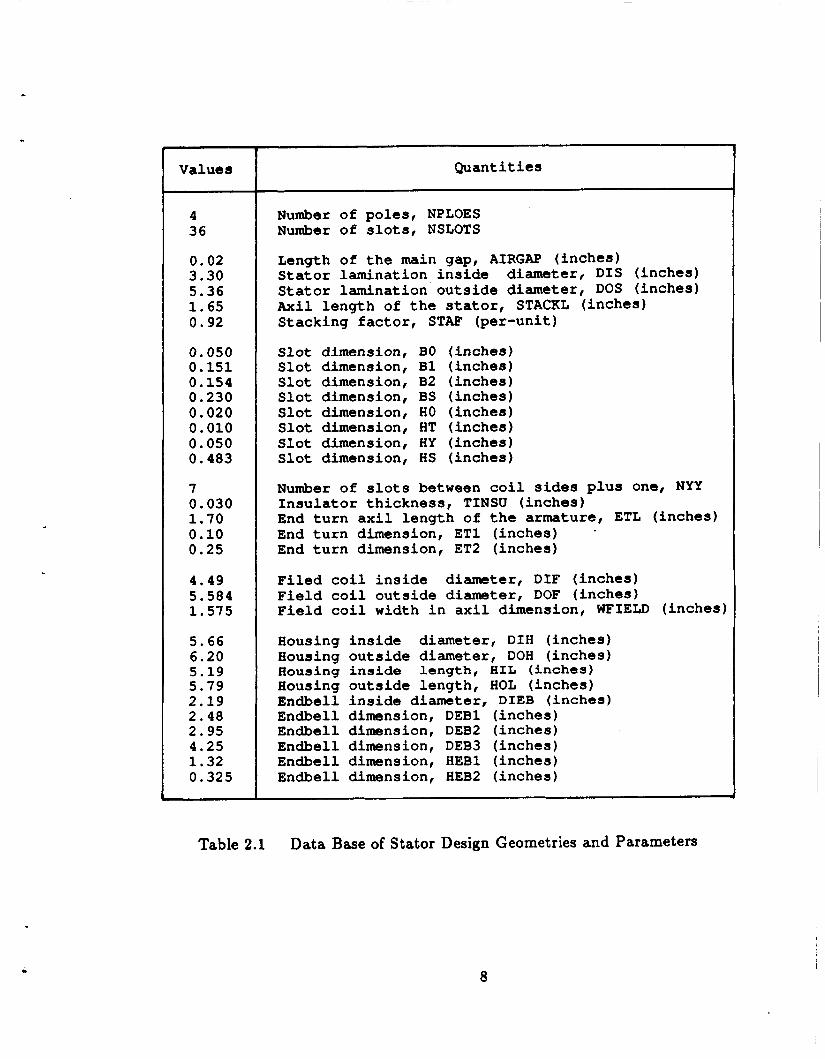
Value a
4 36
0.02 3.30 5.36 1.65 0.92
0.050 0.151 0.154 0.230 0.020 0.010 0.050 0.483
7 0.030 1.70 0.10 0.25
4.49 5.584 1.575
5.66 6.20 5.19 5.79 2.19 2.48 2.95 4.25 1.32 0.325
Quantities
Number of poles, NPLOES Number of slots, NSLOTS
Length of the main gap, AIRGAP (inches) Stator lamination inside diameter, DIS (inches) Stator lamination outside diameter, DOS (inches) Axil length of the stator, STACKL (inches) Stacking factor, STAF (per-unit)
Slot dimension, Slot dimension, Slot dimension, Slot dimension, S1 ot dimension, Slot dimension, S1 ot dimension, Slot dimension,
BO B1 B2 BS HO HT HY HS
(inches) (inches ) (inches ) (inches ) (inches ) (inches 1 (inches 1 (inches )
Number of slots between coil sides plus one, NYY Insulator thickness, TINSU (inches) End turn axil length of the armature, ETL (inches) End turn dimension, ET1 (inches) End turn dimension, ET2 (inches)
Filed coil inside diameter, DIF (inches) Field coil outside diameter, DOF (inches) Field coil width in axil dimension, WFIELD (inches)
Housing inside diameter, DIH (inches) Housing outside diameter, DOH (inches) Housing inside length, HIL (inches) Housing outside length, HOL (inches) Endbell inside diameter, DIEB (inches) Endbell dimension, DEB1 (inches) Endbell dimension, DEB2 (inches) Endbell dimension, DEB3 (inches) Endbell dimension, HEBl (inches) Endbell dimension, HEB2 (inches)
i
Table 2.1 Data Base of Stator Design Geometries and Parameters
8
i
a
I I I I I I I I
2 1
I j - m a I
c s
*! cy
I
.
a
10
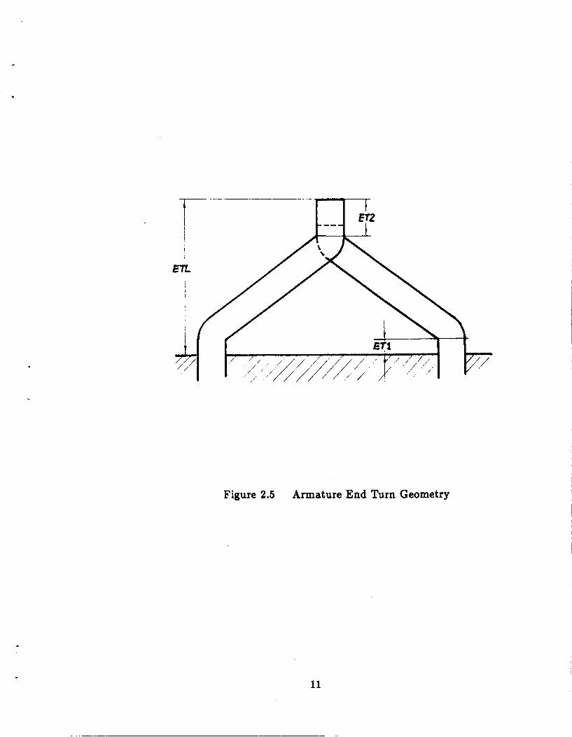
Figure 2.5 Armature End Turn Geometry
11
where the details of the magnetic field distribution are not critical to the overall
performance as was mentioned above. performance as was mentioned above.
The example 14.3 kVA MLA machine decribed above is a four pole alternator
with symmetrical three phase armature windings. The structure of the magnetic
circuit geometry, the excitation current distribution, as well as the armature current
distribution have an identical nature for each pair of poles of the machine. There-
fore, the magnetic field disribution in the machine must have the same symmetric
property for each pair of poles. This means that the magnetic field calculation may
be performed only within the volumetric region of a pair of poles of the machine
to save computer time. The restriction of the volume of the solution region to a
pair of poles will be used throughout this stage of magnetic field computation in
this research project. Accordingly, one half of the machine volume, which occupies
360 electric degrees, which is equivalent to 180 mechanical degrees in the example
MLA, with total machine axial length, is chosen as our solution region for the finite
element calculation. Thus, the total energy of the magnetic field inside the machine
will be twice as that value calculated from the solution region.
12
3.0 BASIC BUILDING BLOCKS AND NATURE
OF THE FINITE ELEMENT GRIDS
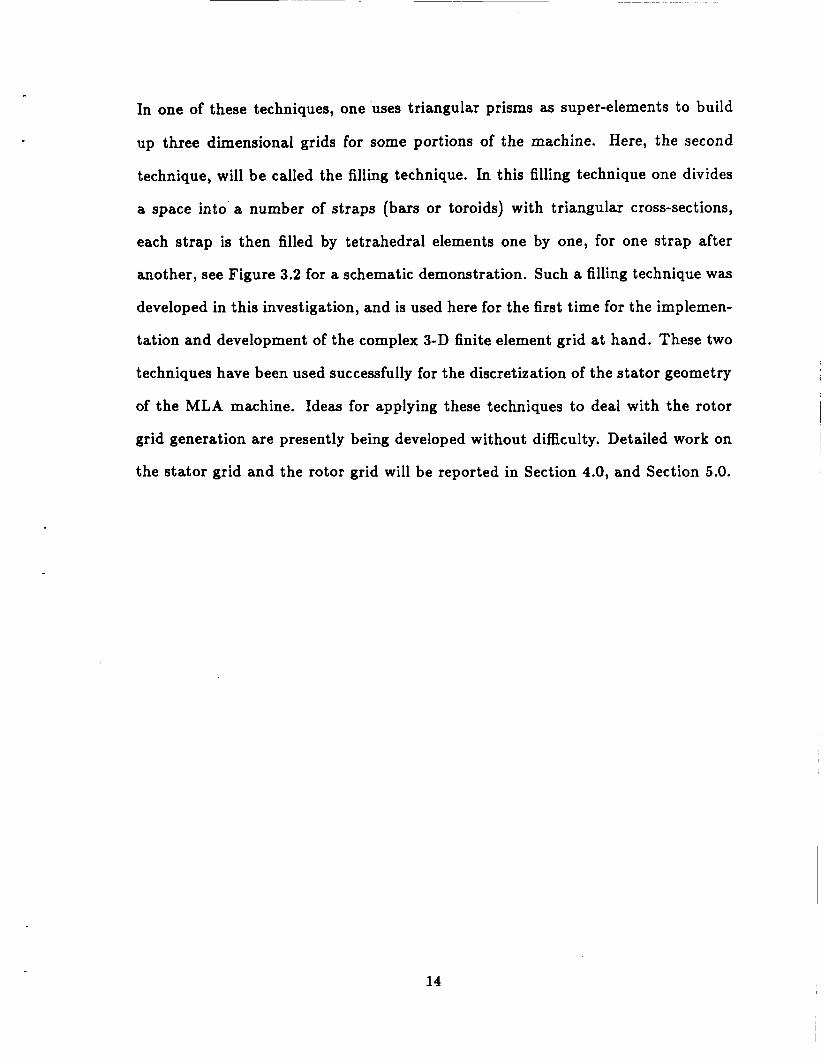
3.1 Tetrahedral Finite Element
To carry out three dimensional finite element computation, the machine ge-
ometry must be discret ized into small three dimensional subregions called finite
elements. Each of these elements is identified through a node-element connection
designation scheme, which will be refered to as the connection matrix of the given
finite element grid. For each element in this three dimensional grid there must be
a material identity number, as well as designated excitation current density com-
ponents, to uniquely represent a particular part of the solution region, with correct
geometry, magnetism, and current source characteristics. Again, these finite el-
ements serves as building blocks to form the three dimensional grid. The basic
building block or finite element used in this investigation is a first order tetra-
hedral element, Figure 3.1. This type of element has been used successfully by
Demerdash et al. in former works of 3-D finite element magnetic field calculation
It is not convenient to directly handle tetrahedra1 elements to buiId up three
dimensional grids because of the difficulty in visulization and computer implemen-
tation for these elements in forming the finite element grid throughout the solution
region. The complex nature of the machine geometry model of the MLA, which
contains the end turn region of the armature winding, as well as extremely difficult
surface geometries of the interfaces between the magnetic poles and the separator
of the rotor, adds substantial difficulties to the discretization work. Two types of
techniques have been used to assist in the generation of the finite element grids.
13
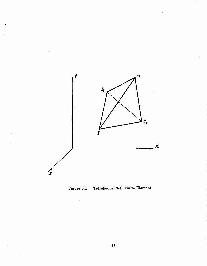
In one of these techniques, one uses triangular prisms as super-elements to build
up three dimensional grids for some portions of the machine. Here, the second
technique, will be called the filling technique. In this filling technique one divides
a space into a number of straps (bars or toroids) with triangular cross-sections,
each strap is then filled by tetrahedral elements one by one, for one strap after
another, see Figure 3.2 for a schematic demonstration. Such a filling technique was
developed in this investigation, and is used here for the first time for the implemen-
tation and development of the complex 3-D finite element grid at hand. These two
techniques have been used successfully for the discretization of the stator geometry
of the MLA machine. Ideas for applying these techniques to deal with the rotor
grid generation are presently being developed without difficulty. Detailed work on
the stator grid and the rotor grid will be reported in Section 4.0, and Section 5.0.
14
/ I
I ,
Y
- x
Figure 3.1 Tetrahedral 3-D Finite Element
15
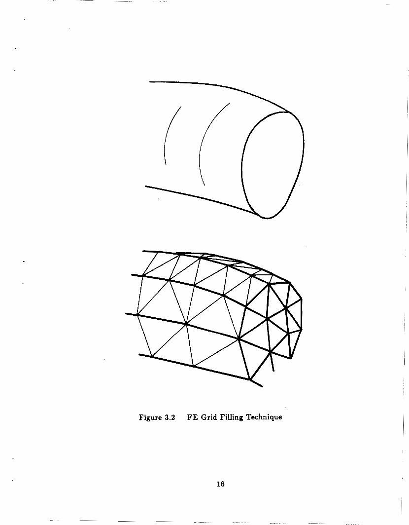
Figure 3.2 FE Grid Filling Technique
16
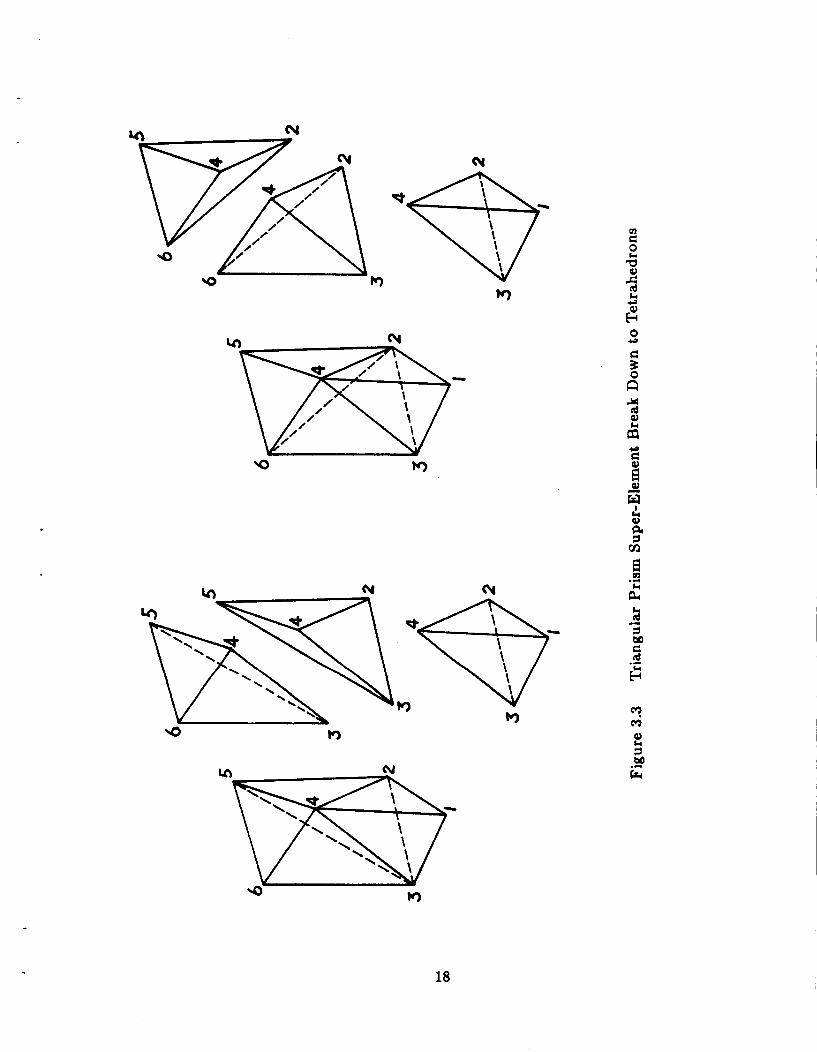
3.2 Triangular Prism Super-Elements
As an aid in constructing the various portions of the finite element grid for some
parts of the machine geometry, triangular prisms are developd as super-elements
to help discretize the three dimensional space for the first step in the process of
generation of the global three dimensional tetrahedral finite element grid. Each
of these triangular prisms is then divided into three tetrahedrons to complete the
grid topology. There are two basic ways to divide a triangular prism into three
tetrahedrons, as shown in Figure 3.3. AIternately using these two types of super-
elements makes it possible to avoid crossing of edges of tetrahedrons from two
super-elements, which might happen at the interfaces, and which must not take
place in a 3-D finite element grid. A triangular prism can be itself a finite element.
However, because of the restrictions on geometric shapes which are ammenable to
discretization by prism shapes, these investigators restricted the use of prisms to
the task (technique) of assisting in the generation of the grid in tetrahedral elements
form. The final grid model of the machine, which is described by a generated data
structure set, is based on tetrahedrons as the basic building blocks.
Using a triangular prism or even considering two triangular prisms forming
one hexahedral block as a super-element, is a very efficient and convenient way
to construct the necessary three dimensional grids. Many machine parts such
as the field coil, the housing, and the rotor shaft, can be cut into pieces with
a number of planes or surfaces carrying identical surface triangular grids. Then
three dimensional triangular prisms can be filled into the space separating the two
surfaces by simply taking one triangle from each of the concerned surfaces to form a
triangular prism in which the top base and the bottom base are the aforementioned
two triangles, and the process is repeated throughout the space between the two
17
Y
d M
18
surfaces, However,there are some circumstances in which the triangular prism
super-elements are not suitable. For example, when elements must be filled into
a gap between two machine parts, where the two surfaces of the gap have arbi-
trary surface triangular patterns, the above method will not work. Thus a filling
technique must be developed to tackle these difficulties. This is described next.
3.3 Filling Technique
As mentioned previously, a filling technique has been developed to generate the
tetrahedral fineite element grids where triangular prisms can not be used effectively.
The main idea of this technique is that one can fill tetrahedrons one after another
into a triangular strap (a bar or toroid with triangular cross-section) when two
side walls (or surfaces) of this strap have been already discretized into arbitrary
triangular grids. After one strap is fully filled with tetrahedrons, the third side wall
of the strap automatically becomes discretized into a certain pattern of a triangular
surface grid, which will be in turn used to determine the tetrahedral finite element
filling manner of the adjacent strap. Such a filling process will be further explaind
by an example later in this section.
Actually, it is not necessary to use this filling technique thoughout the whole
machine geometry, because many parts of the machine can be discretized easily by
triangular prism super-elements from which tetrahedral finite elements are gener-
ated. The whole grid structure can be completed by first building several small grid
modules separately with super-elements then connecting the modules together by
the above mentioned filling technique. This filling technique has been found very
useful1 in matching the stator grid and the rotor grid to complete a global tetra-
19
hedral finite element grid for the class of alternators at hand. Such a matching
is important because the magnetic field calculation will have to be performed at
different rotor positions, to include the effects of rotor geometry and stator slotting
on machine parameters and other performance characteristics.
The following is an example of the application of the above mentioned filling
technique. Consider the geometry given in Figure 3.4, a gap between two surfaces,
with fixed surface triangular grids on each, is to be filled with tetrahedral elements.
In order to apply the filling process, the space of the gap is separated into five straps
as shown in the lower part of Figure 3.4. Each of the straps has one of its three side
walls (surfaces) with a given set of surface triangles. These straps (bars) will then
have to be filled with tetrahedral elements one strap after another, by repeatedly
calling a computer subroutine. Since this subroutine is developed in a manner
suited for general use, it requires that the strap undergoing the tetrahedral filling
process must have two side walls already with given surface triangular grids.
Thus, before the subroutine is called, one side wall, SI, of the first strap,
which must not be the interface with the second strap, as shown in Figure 3.4, has
to be discretized into a suitable set of triangles. At the end of the execution of
the subroutine processing the first strap, a surface triangular grid will have been
established on the third wall (surface), S3, of the strap (bar), which is the interface
between the first strap (bar), 1, and the second strap (bar), 2, see the Figure 3.4.
At that stage, the second strap is ready with surface triangular grids on two of its
three side walls. The second strap is then put through the same process by calling
the same subroutine as is explained above for the first one. The third, the fourth,
and the fifth straps (bars), see Figure 3.4, will have been filled with tetrahedral
elements by sequential application of the above procedure in a chain manner.
20
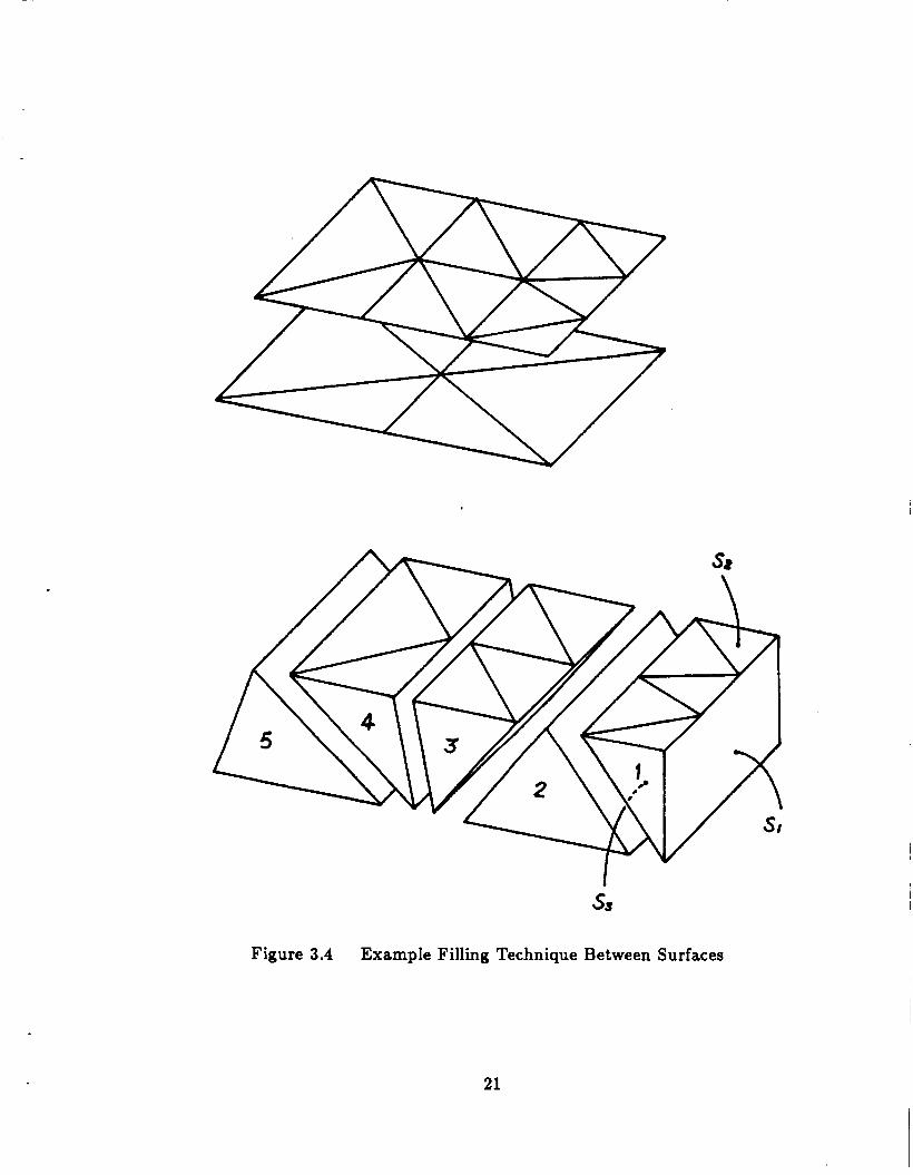
SS
Figure 3.4 Example Filling Technique Between Surfaces
21

The resulting grid which fills the gap of Figure 3.4 with tetrahedral elements is
shown in Figure 3.5.
Next, consider the first strap (bar) in Figure 3.4 as an example to demenstrate
how a tetrahedral grid is computer generated to fill the bar volume under consider-
ation. Let one imagine that this strap is now put in an upright position as shown in
Figure 3.6, graphs (1) through (3), for the convenience of visualization. The front
side wall (surface) with nodes 1, 7, 8,9, and 2 is the wall without a given triangular
grid. Each tetrahedron will be generated by a sequential procedure which can be
generally summarized as follows:
1. Chose a triangular base for the tetrahedron,
2. Find a new node as the fourth vertex of the tetrahedron,
3. Link the new node to each vertex on the base to complete
a tetrahedron.
Applying the three steps given above, the triangle with nodes, 1, 7, and 3, desig-
nated by (1,7,3,1), Figure 3.6, graph (3), is chosen as the base for the first tetrahe-
dron. A searching process is then carried out, which shows that triangle (1,3,4,1)
and triangle (3,7,4,3), Figure 3.6, graph (3), share edges, 1-3, and 3-7, with the
triangular base (1,7,3,1), respectively. Thus, from this information, only node, 4, is
eligible to be the new vertex of the tetrahedron being formed. Accordingly, nodes
1, 7, 3, and 4, make the first tetrahedral element (1,7,3,4}, as shown in Figure 3.6,
graph (4). Node, 4, then takes place of node, 3, to make a new triangular base
(1,7,4,1) for the second tetrahedron under formation.
Repeating the same searching process as explained above for the first tetrahe-
dron, triangle (1,4,2,1) and triangle (4,7,8,4) are found to share edges, 1-4, and
22
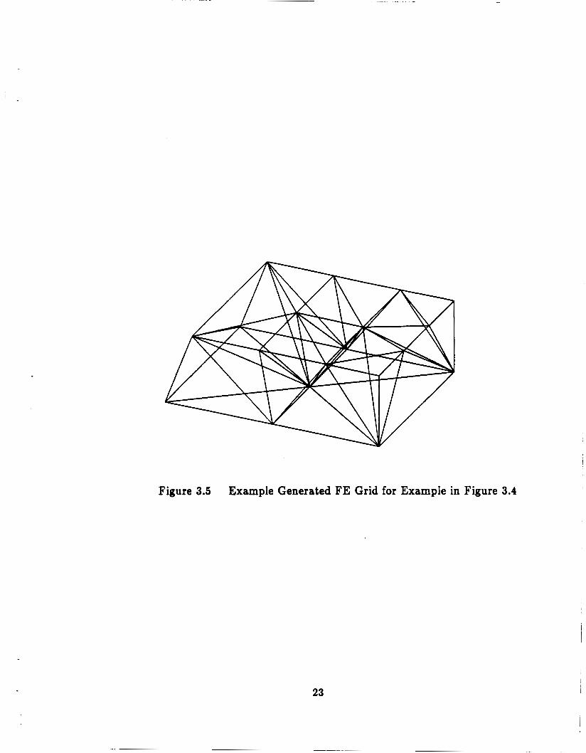
Figure 3.5 Example Generated FE Grid for Example in Figure 3.4
23

h 0.
h 0.
oq h
n - 9 w
h
9 2
h
u?
E m
h
u ts
24
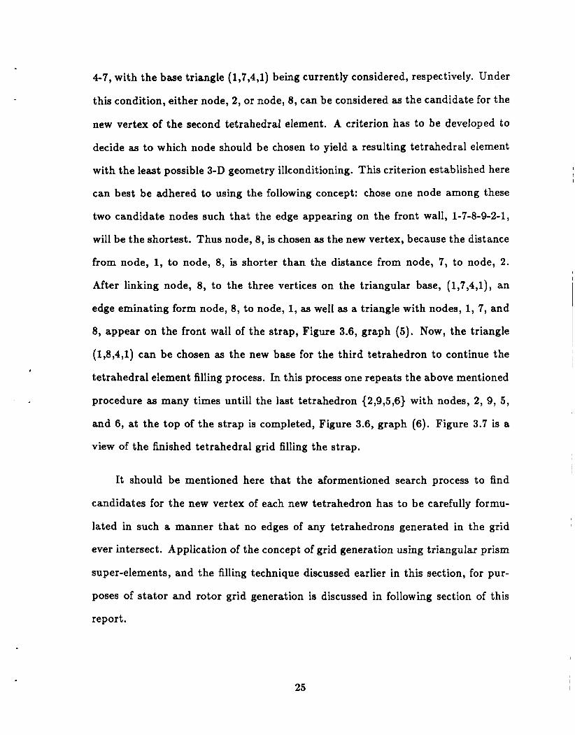
4-7, with the base triangle ( 1,7,4,1) being currently considered, respectively. Under
this condition, either node, 2, or node, 8, can be considered as the candidate for the
new vertex of the second tetrahedral element. A criterion has to be developed to
decide as to which node should be chosen to yield a resulting tetrahedral element
with the least possible 3-D geometry illconditioning. This criterion established here
can best be adhered to using the following concept: chose one node among these
two candidate nodes such that the edge appearing on the front wall, 1-7-8-9-2-1,
will be the shortest. Thus node, 8, is chosen as the new vertex, because the distance
from node, 1, to node, 8, is shorter than the distance from node, 7, to node, 2.
After linking node, 8, to the three vertices on the triangular base, (1,7,4,1), an
edge eminating form node, 8, to node, 1, as well as a triangle with nodes, 1, 7, and
8, appear on the front wall of the strap, Figure 3.6, graph (5). Now, the triangle
(1,8,4,1) can be chosen as the new base for the third tetrahedron to continue the
tetrahedral element filling process. In this process one repeats the above mentioned
procedure as many times until1 the last tetrahedron {2,9,5,6) with nodes, 2, 9, 5,
and 6, at the top of the strap is completed, Figure 3.6, graph (6). Figure 3.7 is a
view of the finished tetrahedral grid filling the strap.
It should be mentioned here that the aformentioned search process to find
candidates for the new vertex of each new tetrahedron has to be carefully formu-
lated in such a manner that no edges of any tetrahedrons generated in the grid
ever intersect. Application of the concept of grid generation using triangular prism
super-elements, and the filling technique discussed earlier in this section, for pur-
poses of stator and rotor grid generation is discussed in following section of this
report.
25
6
8
7
Figure 3.7 Final Triangular Bar FE Tetrahedral Discretization
26

4.0 STATOR FINITE ELEMENT GRID GEOMETRY
According to the flow chart discussed earlier in Section 1.0, which shows the
sequential order of algorithms to be developed in the course of this investigation, the
stator finite element grid is to be generated first, followed by a rotor grid to which
it is to be “stitched” to form the desired global grid system. The selection of the
various rotor positions is dictated by the nature of the performance characteristics
being investigated, as will be explained later in this and future reports.
A cylindrcal surface, which has the same diameter as that in the middle of
the main airgap, and axially extends to both ends of the machine magnetic circuit,
is considered to divide the machine geometry into two parts. The outer part is a
cylindrical shell which contains the armature, half the cylintrical shell constituting
the main airgap, the outer frame and a portion of the endbell, and it occupies
the volumetric region belonging to the stator. This volumetric region is called the
stator grid. Meanwhile, the inner part is an inner cylindrical shell which contains
the rotor, the remaining half of the cylindrical shell of the main airgap, and the
remaining portion of the endbell, and it occupies the volumetric region belonging
to the rotor. This volumetric region is called the rotor grid.
The stator grid and the rotor grid are then generated separately to occupy
these two aforementioned volumetric regions. The inner surface discretization of
the stator grid, as viewed from the rotor side, will have been formed in this inves-
tigation in such a way that the stator grid and the rotor grid can be connected
easily at each of the various rotor positions under consideration.
A computer program using standard Fortran-77 language has been developed
27

successfully to generate the stator finite element grid. The features of the sta-
tor finite element grid, the generated grid pictures, as well as some programming
considerations are reported in this section.
4.1 Basic Grid Module for the Stator Grid
An overview of the configuration of the MLA machine shows that the geometry
of the stator part has symmetric properties as follows; the geometry construction
in each slot pitch of the machine is identical, and the stator has a mirror symmetry
structure with respect to a radial cross-sectional plane at the mid point of the
machine (perpendicular to its axis of rotation). These properties allow one to build
the stator grid by assembling small grid modules with identical finite element grid
topology. Such a consideration of using a small grid module has greatly reduced
the work for the generation of the stator finite element grid.
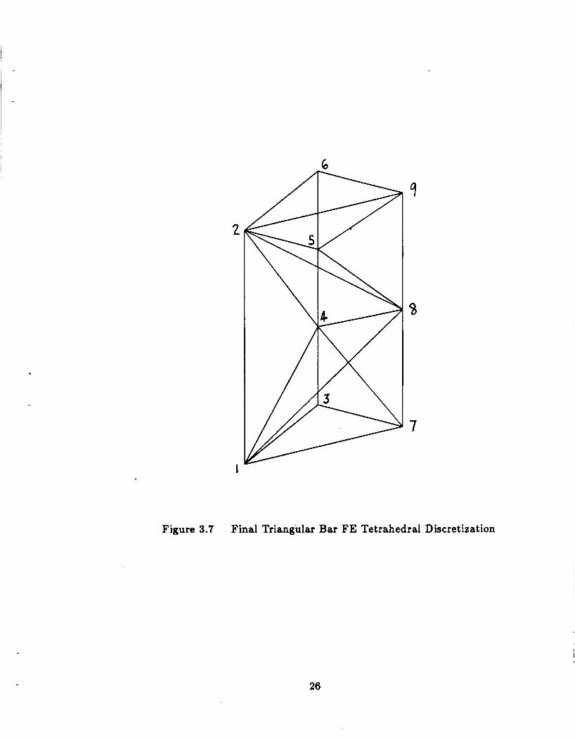
Figure 4.1 shows an isometric view for our basic building block, or grid module,
for the stator finite element grid. This module occupies a space volume within one
slot pitch and half an axial length of the machine, that is, it occupies a region
starting at the outer boundary of the endbell and ending in the middle of the
stator laminations (stack). The front surface which contains cross-sections of the
end turns and field windings as shown in Figure 4.1, and the back surface which
is hidden in this figure, have the same surface discretization, that is the same
triangular pattern. Thus, as many numbers of these modules as deemed necessary
can be put together, side by side in the circumferential direction to accumulate the
stator grid, without any grid geometry conflict at the interface between adjancent
modules. The grid is then mirror imaged into another half length of the machine
28
u U s? 'ii " \
Y
29

to complete the whole stator finite element grid model.
As identified in Figure 4.1, such a grid module has included all machine parts,
insulators, and free spaces in the occupied volumetric region. In this finite element
grid module, each tetrahedral element has a material identity number, and elements
of the same machine part have the same material identity number. Thus, after the
overall stator grid is completed, each machine part can be presented by picking
up all of its tetrahedral elements from the grid, based upon the material number
uniquely assigned to that machine part.
The field winding and the armature winding may carry currents. The relative
magnitude and the direction of the current density vector distributions in each
concerned element have to be generated for utilization in further finite element
computations. This process is to be repeated for the various machine load con-
ditions. More detailed work about the generation of the tetrahedral grid for this
stator grid module of Figure 4.1 will be shown soon in Section 4.3.
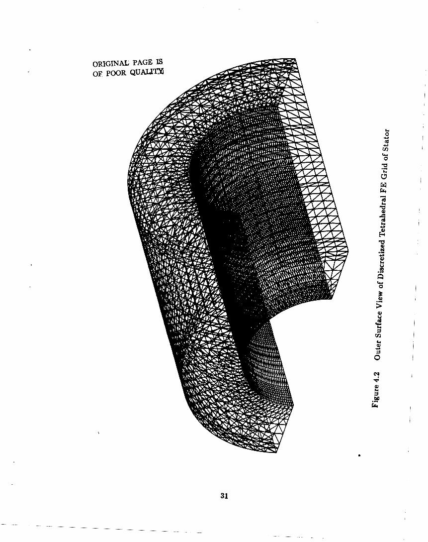
An outer surface view of the generated stator finite element grid is presented
in Figure 4.2. Notice that no internal grid lines are shown in this figure, and that
all the triangles shown represent faces of tetrahedrons in the finite element grid
whose side surfaces lie along these outer surface boundaries of the stator grid. This
finite element grid model covers the geometric space of two pole pitches of the
machine, which is chosen as the solution region for the magnetic field computation,
as mentioned previously in Sestion 2.0.
Notice that the surface discretization on the inner cylindrical surface of the
stator grid, as shown in Figure 4.2, can be considered as a combination of small
rectangles, with each rectangle subdivided into two triangles. It should be pointed
30
ORIGINAL OF, P W R
31
out that the partition for these rectangles in the circumferential direction is uni-
form. Thus, a rotor grid, which will be generated with the same surface dicretiza-
tion on its outer cylinder, can be connected to the stator grid by sharing the nodes
and triangles on the interface. Therefore, such connections can be made at dif-
ferent rotor positions by rotating the rotor grid over one or any whole number of
part it ion distances.
4.2 Stator Grid Presentation
In this section, a number of isometric pictures will be shown to further clarify
the nature of the developed stator finite element grid. The basic computer graphics
tool used to plot these grids is the IGL library of subroutines, a commonly used
graphics software package available recentely in most main frame computer sys-
tems. Frotran programs were developed to employ the basic graphics subroutines
from IGL to plot these 3-D tetrahedral element grids. These computer plotting
routines have capabilities as follows:
1. Plotting of overall 3-D tetrahedral grid with inside lines.
2. Plotting of portions of the grid with a common element material
identity number, with inside lines.
3. Plotting of surface triangular grids, where each surface is a plane
parallel to the XOY, YOZ, or the XOZ coordinate reference plane,
It can also plot a cylindrical surface with its axis of symmetry
coinciding with the Z-axis.
4. Plotting of surface triangular grids, where the surfaces are the
interfaces between regions with different materials.
32
The plotting methods listed above can basically meet the requirements of
graphical display and presentation of the 3-D grid geometries at hand, as will
be shown in the following pages of this report. However, sophisticated graphics
software and hardware, for example, deleting hidden lines, and color pictures, are
needed to obtain high quality 3-D grid pictures. The following are the isometric
pictures which can best represent the generated tetrahedral finite element grid for
the stator geometry at the present status of this investigation:
a) Figure 4.3 shows the grid portion covering the laminated armature core.
All inside lines and the triangles on stator slot walls were eliminated.
b) Figure 4.4 is the portion of the grid covering the armature core over a region
of one slot pitch. It is a portion of the aforementioned basic stator building block
module in Figure 4.1.
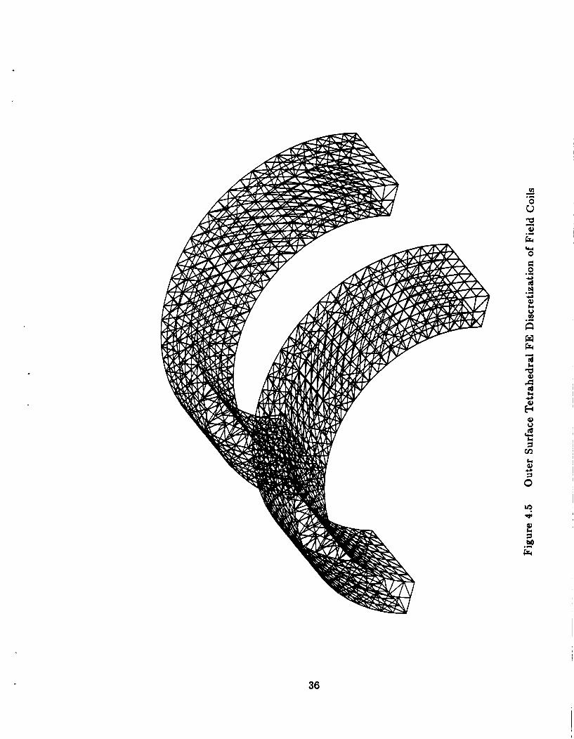
c) Figure 4.5 represents the portion of the stator grid which covers the field
windings of the machine. The inner grid lines were eliminated in this plot.
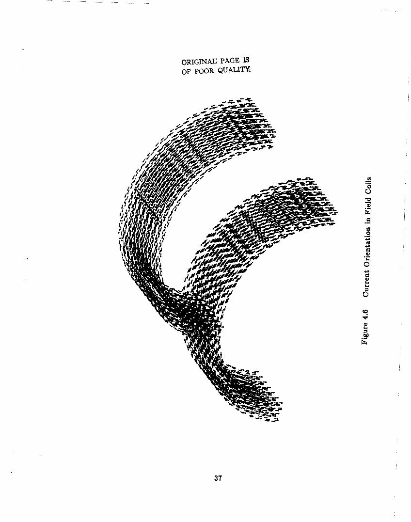
d) Figure 4.6 shows groups of small arrows representing the excitation current
density vectors in the field windings. Each arrow starts from the center of a tetra-
hedral element, pointing in the direction of the current density vector at the center
(centroid) of that element, with a length for each arrow which is proportional to
the magnitude of the current density at that centroid.
e) Figure 4.7 shows the finite element grid for the portion of the volume cov-
ering an armature coil. Such a grid geometry duplicates the physical geometry of
the armature coil of the machine in the three dimensional space. As can be seen
from this picture, it includes the straight line part which is actually embeded in
33

ORIGINAL PAGE IS CE W R QUALITY
d N c;,
V v)
.C(
E
c1 .C(
34
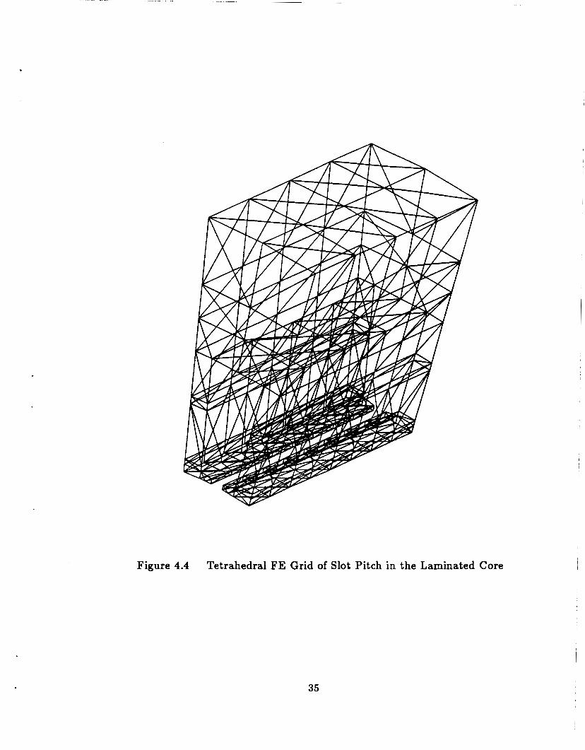
Figure 4.4 Tetrahedral FE Grid of Slot Pitch in the Laminated Core
35
v1 d .e
0 V
36
0RIGINA.C PAGE IS OF POOR Q U A L I ~ J
m
0 V c( .d
37

c rd
0 rcr
w cr
38

the armature laminations (slots), as well as the end turn part of the coil which
forms the coil side connection from one slot to its corresponding return coil side to
form a complete coil. Upon closer examination of Figure 4.7, one can recogonize
that the right portion and the left portion of the coil shown in the figure are in
different layers of the armature winding. That is, one side is in the upper layer and
the other side is in the lower layer of the armature winding.
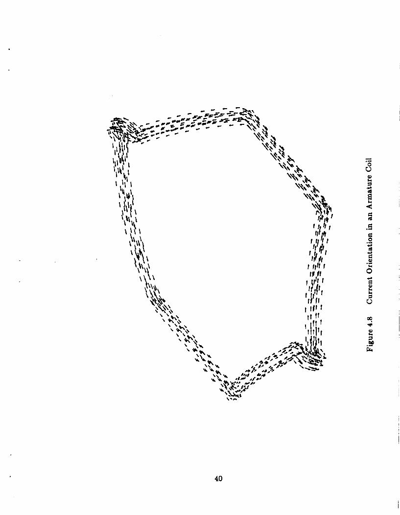
f ) Figure 4.8 indicates the current density vector distributions inside an ar-
mature coil. Again, these arrows represent both the directions and the relative
magnitudes of the current density distribution, as explained earlier for the case of
the field winding in Figure 4.6.
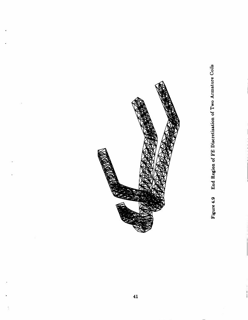
g) Figure 4.9 displays a picture which shows how two armature coils overlap
in the end turn region of the armature.
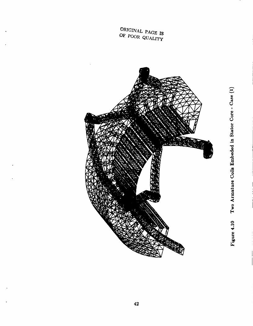
h) Figure 4.10 presents the portion of the grid covering the laminated armature
core as well as some armature coils with their straight line portions embeded in
the stator slots. All inside lines of the grid for laminated core were eliminated.
However, the inner lines in the coils were not eliminated to highlight the differences
between the core and coil regions.
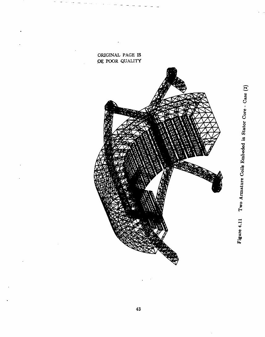
i) Figure 4.11 is another view for the same grid as shown above in Figure 4.10.
and
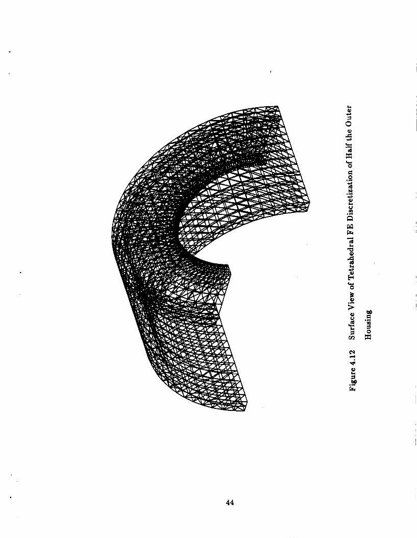
j) Figure 4.12 shows the portion of the stator grid covering the housing part in
the stator magnetic circuit. Only a half portion of the housing is presented here.
In the actual model the finite element grid not only contains the portion shown in
Figure 4.12, but also contains its mirror image.
39
40
E 3
rw 0
W R 0
rw
a W
41
n d W
I
0 V
42
2 2 a P
w W + .d
0 V
P w
BHPPGINAL PAGE IS POOR QUALITY
I
43
I
44
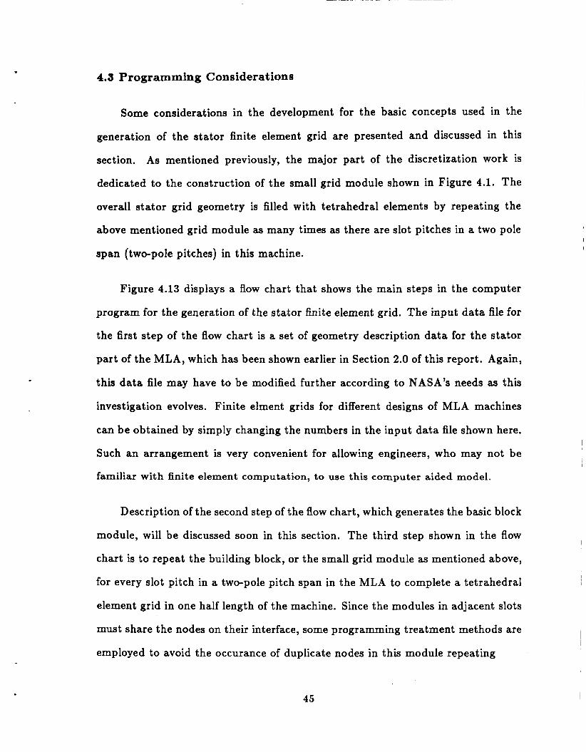
4.3 Programming Considerations
Some considerations in the development for the basic concepts used in the
generation of the stator finite element grid are presented and discussed in this
section. As mentioned previously, the major part of the discretization work is
dedicated to the construction of the small grid module shown in Figure 4.1. The
overall stator grid geometry is filled with tetrahedral elements by repeating the
above mentioned grid module as many times as there are slot pitches in a two pole
span (two-pole pitches) in this machine.
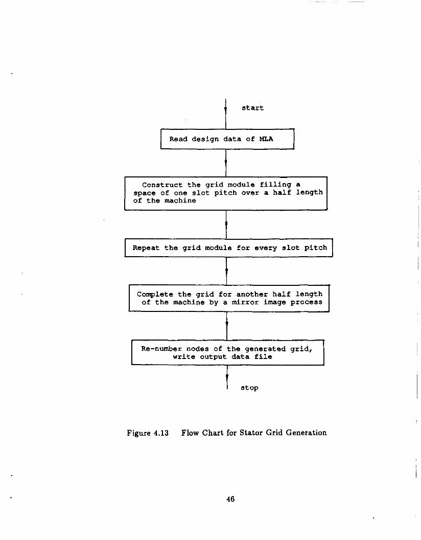
Figure 4.13 displays a flow chart that shows the main steps in the computer
program for the generation of the stator finite element grid. The input data file for
the first step of the flow chart is a set of geometry description data for the stator
part of the MLA, which has been shown earlier in Section 2.0 of this report. Again,
this data file may have to be modified further according to NASA’s needs as this
investigation evolves. Finite elment grids for different designs of MLA machines
can be obtained by simply changing the numbers in the input data file shown here.
Such an arrangement is very convenient for allowing engineers, who may not be
familiar with finite element computation, to use this computer aided model.
Description of the second step of the flow chart, which generates the basic block
module, will be discussed soon in this section. The third step shown in the flow
chart is to repeat the building block, or the small grid module as mentioned above,
for every slot pitch in a two-pole pitch span in the MLA to complete a tetrahedral
element grid in one half length of the machine. Since the modules in adjacent slots
must share the nodes on their interface, some programming treatment methods are
employed to avoid the occurance of duplicate nodes in this module repeating
45
4 s ta r t
Read design d a t a of MLA
I
I
Construct t h e g r i d module f i l l i n g a space of one s l o t p i t c h over a h a l f l ength of t h e machine
I t
I I Repeat t h e g r i d module f o r every s l o t p i t c h
t I Complete t h e g r i d f o r another h a l f l eng th
of t h e machine by a mirror image process
t I Re-number nodes of t h e generated g r i d , I w r i t e output data f i l e
Figure 4.13 Flow Chart for Stator Grid Generation
46
process.
Besides, the material number for the armature coil part in the grid module
is subject to change during this module-repeating work stage. This is because
armature coils in different slots, or in the same slot but different layers, may belong
to a different phase in the armature winding. Hence, they have to be identified
from each other with a numbering, sequence so that the correct phase current
distribution can be assigned later to perform magnetic filed computations under
various machine load conditions.
The next step of the flow chart in Figure 4.13 is to mirror image the grid which
has been generated by the previous steps, to form the stator grid corresponding
to the given machine geometry. The last step of the flow chart is renumbering all
generated nodes for the convenience of the stator-rotor grids connection to form
the global grid. The last step is being presently developed by these investigators.
.
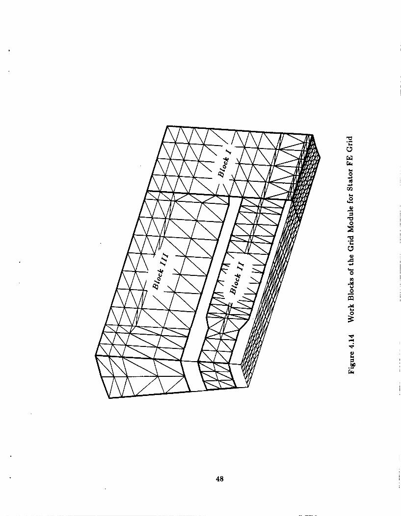
The construction work for the basic building block module of the stator grid is
presented in a picture shown in Figure 4.14. The module is generated by combining
further small work blocks, Block I, Block 11, and Block 111, as shown in Figure
4.14. Instead of building these work blocks in terms of different machine parts,
they are formed according to consideration of the geometry features. This means
that each chosen block has simple geometry structure so that the grid inside the
block can be built up mainly by triangular prism super-elements. Blocks I and
111, as well as Block I and 11, are connected together directly because they can
share common interfaces, respectively. However, Block 11 can not be connected
directly to either Block 111 or to the cylindrical surface in the middle of the main
airgap, which is the bottom surface shown in Figure 4.14. The reason for this is
47
k
cw 0
48
that the grid topology of Block 11 may change due to different designs of the
armature coil pitch, which may be required by further design modification studies
at later stages of this research project. Thus, the filling technique which has been
described in Section 3.0 of this report, is used to complete the tetrahedral grid
between Block 11 and Block 111, that joins the two blocks in the stator grid
module, aa well as the grid between Block 11 and the cylindrical surface at the
middle of the main airgap.
The tetrahedral grid filling Block 11, shown in Figure 4.14, is the most compli-
cated task in the stator finite element grid generation. This block contains complex
geometry of the end turn region of the armature winding, and the dimensions and
topological geometry will change when the design of the armature slot pitch varies.
In order to tackle these difficulties, a further partition for Block 11 was made,
which allows one to build up grids in each small subblock, in Figure 4.15, then
connect them together to complete the grid filling the geometry of Block I I .
Subblock, A, of Block 11 in Figure 4.15 is the geometry portion where the
upper bar and the lower bar of the armature winding exit out of the slot and begin
to bend in opposite directions. Subblock, B1, in Figure 4.15 is the region in which
the upper coil bar and the lower coil bar cross each other. It must be understood
that the upper bar and the lower bar in Subblock, B1, belong to the portions of
two different coils embeded in the slots adjacent to the slot containing Block I I .
Subblock, Bz, in Figure 4.15 has the same geometric nature and grid topology as
those of subblock, B1. If the armature coil pitch increases, more subblocks than
B1 and Bz, with an identical tetrahedral element grid, will have to be used. This is
because the greater the armature coil pitch, the more upper coil bars and lower coil
bars corss each other in the end turn region. Subblock, C, in Figure 4.15 contains
49
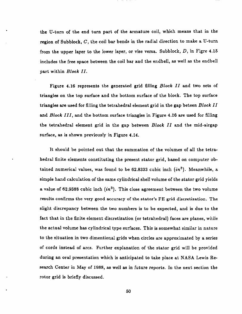
the U-turn of the end turn part of the armature coil, which means that in the
region of Subblock, C, the coil bar bends in the radial direction to make a U-turn
from the upper layer to the lower layer, or vise versa. Subblock, D, in Figre 4.15
includes the free space between the coil bar and the endbell, as well as the endbell
part within Block II.
Figure 4.16 represents the generated grid filling Block 11 and two sets of
triangles on the top surface and the bottom surface of the block. The top surface
triangles are used for filling the tetrahedral element grid in the gap beteen Block 11
and Block 111, and the bottom surface triangles in Figure 4.16 are used for filling
the tetrahedral element grid in the gap between Block 11 and the mid-airgap
surface, as is shown previously in Figure 4.14.
It should be pointed out that the summation of the volumes of all the tetra-
hedral finite elements constituting the present stator grid, based on computer ob-
tained numerical values, was found to be 62.8333 cubic inch (in'). Meanwhile, a
simple hand calculation of the same cylindrical shell volume of the stator grid yields
a value of 62.9388 cubic inch (in'). This close agreement between the two volume
results confirms the very good accuracy of the stator's FE grid discretization. The
slight discrepancy between the two numbers is to be expected, and is due to the
fact that in the finite element discretization (or tetrahedral) faces are planes, while
the actual volume has cylindrical type surfaces. This is somewhat similar in nature
to the situation in two dimentional grids when circles are approximated by a series
of cords instead of arcs. Further explanation of the stator grid will be provided
during an oral presentation which is anticipated to take place at NASA Lewis Re-
search Center in May of 1988, as well as in future reports. In the next section the
rotor grid is briefly discussed.
50
51
I
E
a d w

I
U U
52
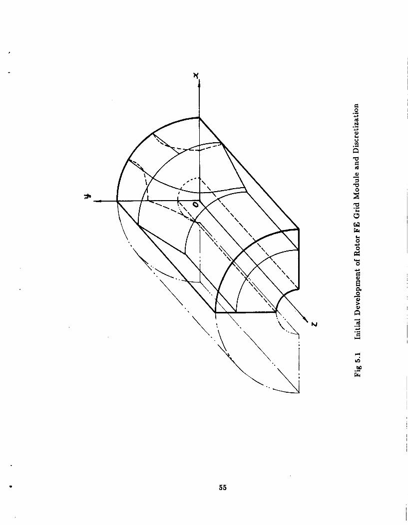
5.0 ROTOR FINITE ELEMENT GRID GEOMETRY
The finite element grid filling the geometry of the rotor is currently being
developed by these investigators. As explained in Section 4.0, the volumetric region
of the rotor grid is a cylindrical shell, which contains the rotor, half of the cylindrical
shell of the main airgap, the miliary airgap, and a portion of the endbell. Since this
rotor grid must be connected to the stator grid, as discussed earlier in Section 4.0,
the outer cylindrical surface of the rotor grid should have the same discretization
as that on the inner cylindrical surface of the stator grid, such that the rotor grid
and the stator grid can be "stiched" together by sharing the nodes and surface
triangles on their cylindrical interface (surface).
According to the symmetry nature of the rotor geometry, a grid module which
fills one octant of the volumetric region of the rotor grid is being generated at
first. Such an octant is shown in the first octant of the 3-D space as displayed
in Figure 5.1. Then a conterpart of this module, which is located in the second
octant of Figure 5.1, is being generated by mirror imaging the grid module in the
first octant, with respect to the Y O 2 referece plane. The remaining portion of
the rotor grid, which is in the fifth and the sixth octants of the 3-D space, will
have been completed by rotating and mirror imaging the grid modules in the first
and the second octants. Namely, this means that one rotates the grid module in
the first octant by (90) mechanical degrees around the Z-axis, then mirror images
it with respect to the XOY reference plane to form the grid in the sixth octant.
Similarly, one rotates the grid module in the second octant by (-90) mechanical
degrees around the Z-axis, then mirror images it with respect to the XOY reference
plane to form the grid in the fifth octant of the 3-D space. The inside geometry
53
of the rotor is a very complicated one. A series of cross-sectional drawings has to
be used to explain the inner details of this complex geometry. Accordingly, the
volumetric octant of the grid module is being cut into pieces, or disks, by a number
of cross-sectional planes, then each of these cross-sectional surfaces is separatly
discretized into triangels. Finally, tetrahedral finite elements are filled into the
pieces, or disks, between these cross-sectional surfaces to complete the rotor grid.
The filling technique discussed in earlier sections of this report will be used as a
main tool for the generation of the rotor grid. Details of this part of the work and
resulting rotor grid will be shown in future reports.
54
k
5: E a c d
cw 0
55
6.0 IMMEDIATE FORTHCOMING EFFORTS
Over the period of the next 6 months, a very brief summary of the tasks ahead
can be listed as follows:
(1) Complete the FE discretization of the rotor portion of the global FE grid
of the MLA Class of machines. That is, complete the rotor FE grid.
(2) Assemble the rotor and stator FE grids to form the global FE grid, and
recheck all geometries and data of the example 14.3 kVA MLA, and experiment
with numerous rotor positions relative to the stator to assure the generality of the
FE discretization for magnetic field computation purposes.
(3) Experiment with geometric parameter change in various parts of windings,
magnetic cores, and airgaps to ascertain the generality of the FE discretization for
purposes of studying various design options.
(4) Attempt a preliminary 3-D FE magnetic field solution at no-load, and
without inclusion of magnetic nonlinearities. That is, obtain the open-circuit airgap
line characteristics of the example 14.3 kVA MLA.
( 5 ) Attempt a saturated nonlinear magnetic field solution of the MLA at sev-
eral field excitations near and above rated open circuit voltage. Compare results
with previous or new data on the open-circuit no-load characteristic of the example
14.3 kVA MLA.
(6) If steps (1) through (5) are complete, proceed to short circuit, zero power
factor, and other load cases. Further steps will be outlined in the second six month
progress report.
56
7.0 CONCLUSIONS
The investigation is proceeding as scheduled at the expected pace. The stator
finite element grid of the MLA class of alternators is now complete, as given earlier
in this report. The rotor FE grid is presently being developed. Both stator and
rotor FE grids, which form the global MLA-FE grid are expected to be reported
on in an oral presentation, which is expected to take place at the NASA-Lewis
Research Center at a date in May 1988 to be agreed upon with NASA Lewis
personnel.
r
W
57

8.0 REFRENCES
I
[ 1 ] Demerdash, N.A., “Computer-Aided Modeling and Prediction of Performance
of the Modified Lundell Class of Alternators in Space Station Solar Dynamic
Power Systems,” Research Proposal submitted to NASA, April 1987.
[ 2 ] Repas, D.S., and Edkin, R.A., “Performance of Characteristics of a 14.3-
Kilovolt-Ampere Modified Lundell Alternator for 1200 Hertz Brayton-Cycle
Space Power System,” N A S A Reprot; NASA-TN-5405, sept. 1969.
[ 3 ] Demerdash, N.A., Nehl, T.W., and Fouad, F.A., “Finite Element Formula-
tion and Analysis of Three Dimensional Magnetic Field Problems,” I E E E
Transactions on Magnetics, Vol. MAG-16, No. 5 , 1980, pp. 1092-1094.
[ 4 ] Demerdash, N.A., Nehl, T.W., Fouad, F.A., and Mohammed, O.A., “Three
Dimensional Finite Element Vector Potential Formulation of Magnetic Fields
in Electrical Apparatus,” I E E E Transactions on Power Apparatus and
Systems, Vol. PAS-100, No. 8, August 1981, pp. 4104-4111.
[ 5 ] Demerdash, N.A., Nehl, T.W., Mohammed, O.A., and Fouad, F.A., “Exper-
imental Verification and Application of the Three Dimensional Finite Ele-
ment Magnetic Vector Potential Method in Electrical Apparatus,” I E E E
Transactions on Power Apparatus and Systems, Vol. PAS-100, No. 8,
August 1981, pp. 4112-4122.
[ 6 ] Mohammed, O.A., Demerdash, N.A., and Nehl, T.W., “Nonlinear Vector Po-
tential Formulation and Experimental Verification of Newton-Raphson Solu-
tion of Three Dimensional Magnetostatic Fields in Electrical Devices,” I E E E
58

Transactions on Energy Conversion, Vol. EC-1, No. 1, 1986, pp. 177-185.
59

![[XLS] · Web viewMAGISTRATE'S NO: 142/04 MPUMALANGA SESI TSHABALALA NGCAMU MANDLA FRANCIS 9044/2004 THEMBISILE CLOROH MANDLA FRANCE 11568/2005 5598/2003 27 Aug 1987 28 Aug 2006 MANDLA](https://static.fdocuments.in/doc/165x107/5aff0a0c7f8b9a68498f1a7b/xls-viewmagistrates-no-14204-mpumalanga-sesi-tshabalala-ngcamu-mandla-francis.jpg)