25.visualization - extra slides - Clarkson...

CS452/552; EE465/505

Scientific Visualization

4-21–15

! Rendering the teapot ! Graphics API support for Curves and Surfaces

✦ Tessellation Shading ✦ Geometry Shading

! Scientific Visualization

Read: Angel, ✦Chapter 11.10, The Utah Teapot ✦Chapter 11.14, Tessellation and Geometry Shaders

Final Exam: Monday, April 27th, 3:15 to 6:15, SC162

Outline

! can export to WebGL ✦ https://blog.mozilla.org/blog/2015/03/03/unity-5-ships-and-

brings-one-click-webgl-export-to-legions-of-game-developers/ ✦ http://docs.unity3d.com/Manual/webgl-building.html ✦ http://www.gamasutra.com/view/news/213459/

Indepth_on_Unity_5s_WebGL_publishing_tech.php

Unity 5

https://blog.mozilla.org/blog/2015/03/03/unity-5-ships-and-brings-one-click-webgl-export-to-legions-of-game-developers/

http://docs.unity3d.com/Manual/webgl-building.html

http://www.gamasutra.com/view/news/213459/Indepth_on_Unity_5s_WebGL_publishing_tech.php

How to Draw Spline Curves

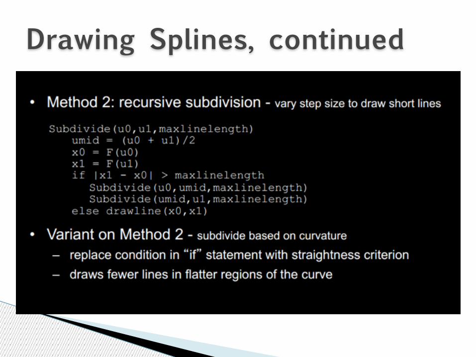
Drawing Splines, continued

Summary

! Look at rendering with WebGL ! Use Utah teapot for examples

✦Recursive subdivision ✦Polynomial evaluation ✦Adding lighting

Rendering the Teapot

Angel and Shreiner: Interactive Computer Graphics 7E © Addison-Wesley 2015

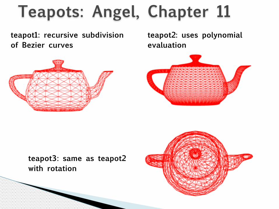
Teapots: Angel, Chapter 11teapot1: recursive subdivision of Bezier curves

teapot2: uses polynomial evaluation

teapot3: same as teapot2 with rotation

Teapots: Angel, Chapter 11teapot5: rotating, uses polynomial evaluation and normals computed for each triangle

teapot4: rotating, uses polynomial evaluation and exact normals

! Most famous data set in computer graphics !Widely available as a list of 306 3D vertices and the indices that define 32 Bezier patches

Utah Teapot


vertices.js

var numTeapotVertices = 306; var vertices = [ vec3(1.4 , 0.0 , 2.4), vec3(1.4 , -0.784 , 2.4), vec3(0.784 , -1.4 , 2.4), vec3(0.0 , -1.4 , 2.4), vec3(1.3375 , 0.0 , 2.53125), . . . ];


patches.jsvar numTeapotPatches = 32; var indices = new Array(numTeapotPatches); indices[0] = [0, 1, 2, 3, 4, 5, 6, 7, 8, 9, 10, 11, 12, 13, 14, 15 ]; indices[1] = [3, 16, 17, 18, . . ];


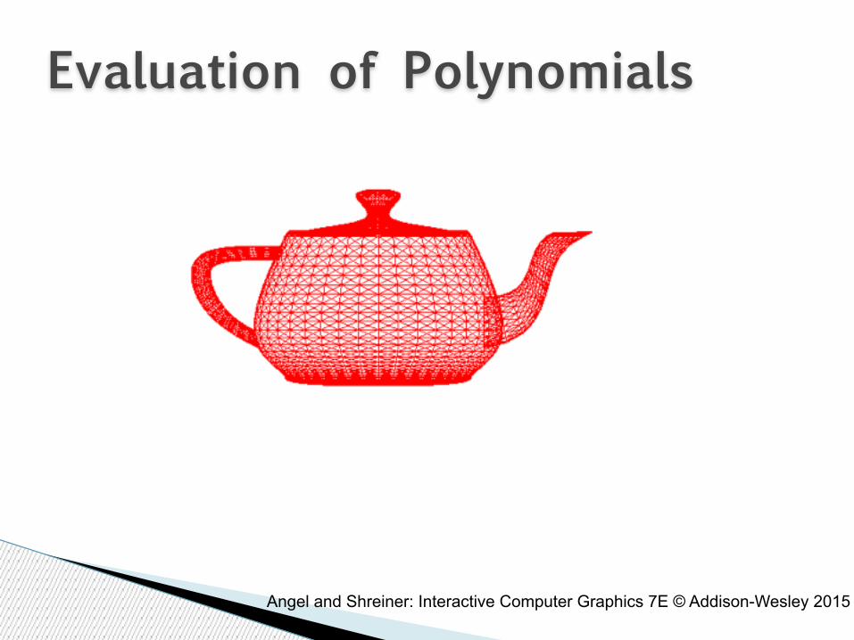
Evaluation of Polynomials


Bezier Functionbezier = function(u) { var b = []; var a = 1-u; b.push(u*u*u); b.push(3*a*u*u); b.push(3*a*a*u); b.push(a*a*a); return b; }


Patch Indices to Data var h = 1.0/numDivisions;

patch = new Array(numTeapotPatches); for(var i=0; i<numTeapotPatches; i++) patch[i] = new Array(16); for(var i=0; i<numTeapotPatches; i++) for(j=0; j<16; j++) { patch[i][j] = vec4([vertices[indices[i][j]][0], vertices[indices[i][j]][2], vertices[indices[i][j]][1], 1.0]); }


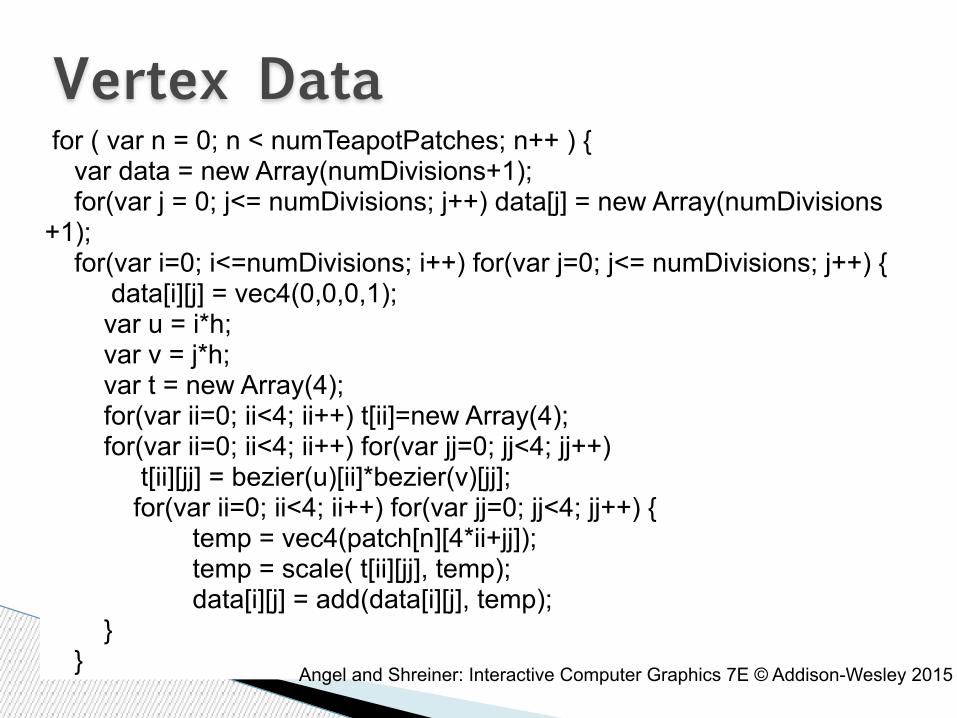
Vertex Data for ( var n = 0; n < numTeapotPatches; n++ ) { var data = new Array(numDivisions+1); for(var j = 0; j<= numDivisions; j++) data[j] = new Array(numDivisions+1); for(var i=0; i<=numDivisions; i++) for(var j=0; j<= numDivisions; j++) { data[i][j] = vec4(0,0,0,1); var u = i*h; var v = j*h; var t = new Array(4); for(var ii=0; ii<4; ii++) t[ii]=new Array(4); for(var ii=0; ii<4; ii++) for(var jj=0; jj<4; jj++) t[ii][jj] = bezier(u)[ii]*bezier(v)[jj]; for(var ii=0; ii<4; ii++) for(var jj=0; jj<4; jj++) { temp = vec4(patch[n][4*ii+jj]); temp = scale( t[ii][jj], temp); data[i][j] = add(data[i][j], temp); } } Angel and Shreiner: Interactive Computer Graphics 7E © Addison-Wesley 2015

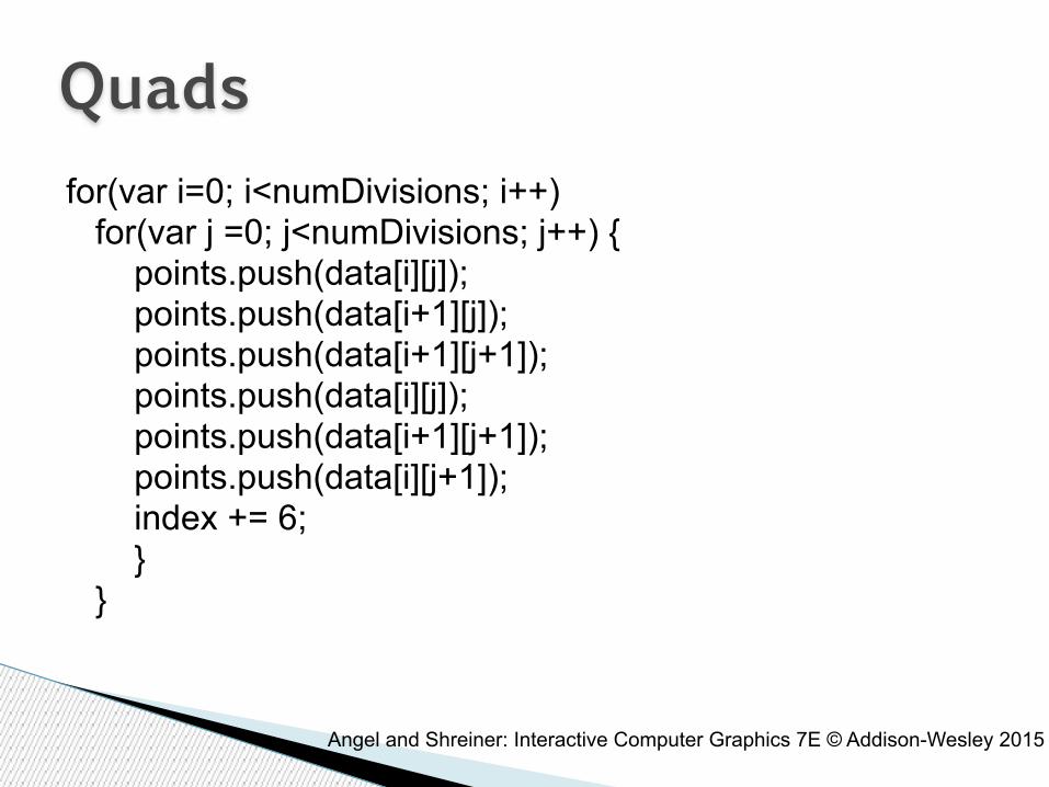
Quads for(var i=0; i<numDivisions; i++) for(var j =0; j<numDivisions; j++) { points.push(data[i][j]); points.push(data[i+1][j]); points.push(data[i+1][j+1]); points.push(data[i][j]); points.push(data[i+1][j+1]); points.push(data[i][j+1]); index += 6; } }


Recursive Subdivision


Divide CurvedivideCurve = function( c, r , l){ // divides c into left (l) and right ( r ) curve data var mid = mix(c[1], c[2], 0.5); l[0] = vec4(c[0]); l[1] = mix(c[0], c[1], 0.5 ); l[2] = mix(l[1], mid, 0.5 ); r[3] = vec4(c[3]); r[2] = mix(c[2], c[3], 0.5 ); r[1] = mix( mid, r[2], 0.5 ); r[0] = mix(l[2], r[1], 0.5 ); l[3] = vec4(r[0]); return; }


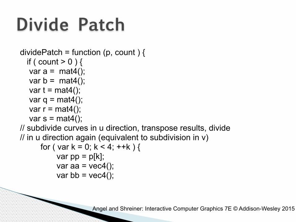
Divide PatchdividePatch = function (p, count ) { if ( count > 0 ) { var a = mat4(); var b = mat4(); var t = mat4(); var q = mat4(); var r = mat4(); var s = mat4(); // subdivide curves in u direction, transpose results, divide // in u direction again (equivalent to subdivision in v) for ( var k = 0; k < 4; ++k ) { var pp = p[k]; var aa = vec4(); var bb = vec4();


Divide Patch divideCurve( pp, aa, bb ); a[k] = vec4(aa); b[k] = vec4(bb); } a = transpose( a ); b = transpose( b ); for ( var k = 0; k < 4; ++k ) { var pp = vec4(a[k]); var aa = vec4(); var bb = vec4(); divideCurve( pp, aa, bb ); q[k] = vec4(aa); r[k] = vec4(bb); } for ( var k = 0; k < 4; ++k ) { var pp = vec4(b[k]); var aa = vec4();


Divide Patch var bb = vec4(); divideCurve( pp, aa, bb ); t[k] = vec4(bb); } // recursive division of 4 resulting patches dividePatch( q, count - 1 ); dividePatch( r, count - 1 ); dividePatch( s, count - 1 ); dividePatch( t, count - 1 ); } else { drawPatch( p ); } return; }


Draw PatchdrawPatch = function(p) { // Draw the quad (as two triangles) bounded by // corners of the Bezier patch points.push(p[0][0]); points.push(p[0][3]); points.push(p[3][3]); points.push(p[0][0]); points.push(p[3][3]); points.push(p[3][0]); index+=6; return; }


Adding Shading


Using Face Normals var t1 = subtract(data[i+1][j], data[i][j]); var t2 =subtract(data[i+1][j+1], data[i][j]); var normal = cross(t1, t2); normal = normalize(normal); normal[3] = 0; points.push(data[i][j]); normals.push(normal); points.push(data[i+1][j]); normals.push(normal); points.push(data[i+1][j+1]); normals.push(normal); points.push(data[i][j]); normals.push(normal); points.push(data[i+1][j+1]); normals.push(normal); points.push(data[i][j+1]); normals.push(normal); index+= 6;


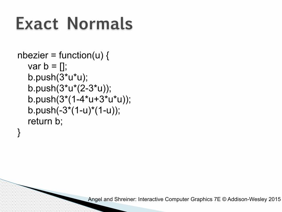
Exact Normalsnbezier = function(u) { var b = []; b.push(3*u*u); b.push(3*u*(2-3*u)); b.push(3*(1-4*u+3*u*u)); b.push(-3*(1-u)*(1-u)); return b; }


! Basic limitation on rasterization is that each execution of a vertex shader is triggered by one vertex and can output only one vertex

! Geometry shaders allow a single vertex and other data to produce many vertices

! Example: send four control points to a geometry shader and it can produce as many points as needed for Bezier curve

Geometry Shader


! Can take many data points and produce triangles

! More complex since tessellation has to deal with inside/outside issues and topological issues such as holes

! Neither geometry or tessellation shaders supported by ES

! ES 3.1 (just announced) has compute shaders

Tessellation Shaders


Scientific Visualization

! Scalar fields (3D volume of scalars) ■ e.g. x-ray densities (MRI, CT scan)

! Vector fields (3D volume of vectors) ■ e.g. velocities in a wind tunnel

! Tensor fields (3D volume of tensors [matrices]) ■ e.g. stresses in a mechanical part

! Static or dynamic over time

Types of Data

Outline! Height Fields and Contours ! Scalar Fields ! Volume Rendering ! Vector Fields

Height Field

See Angel, Color Plate 25 Elevation data for Honolulu, Hawaii

Meshes

Contour Curves

Marching Squares

Interpolating Intersections

Cases for Vertex Labels

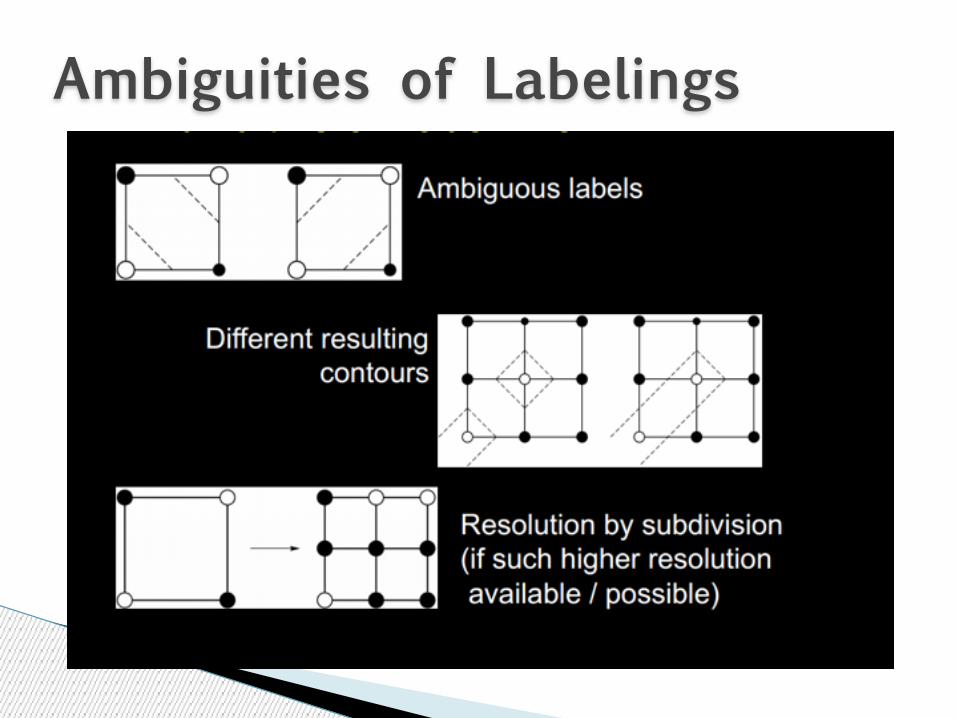
Ambiguities of Labelings

Marching Squares Example

Scalar Fields

Isosurfaces

Marching Cubes

Marching Cube Tessellations

Volume Rendering

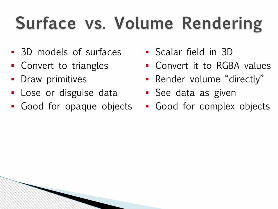
■ 3D models of surfaces ■ Convert to triangles ■ Draw primitives ■ Lose or disguise data ■ Good for opaque objects

Surface vs. Volume Rendering■ Scalar field in 3D ■ Convert it to RGBA values ■ Render volume “directly” ■ See data as given ■ Good for complex objects

! Medical ✦Computed Tomography (CT) ✦Magnetic Resonance Imaging (MRI) ✦Ultrasound

! Engineering and Science ✦Computational Fluid Dynamic (CFD) ✦Aerodynamic simulations ✦Meterorology ✦Astrophysics

Sample ApplicationsSee Angel, Color Plate 20 Volume Rendering of CT data

Volume Rendering Pipeline

Transfer Functions

Transfer Function Example

See Angel, Color Plate 19 Fluid dynamics of the Earth’s mantle

! Three volume rendering techniques ■ Volume ray casting ■ Splatting ■ 3D texture mapping

! Ray Casting ■ Integrate color through volume ■ Consider lighting (surfaces?) ■ Use regular x,y,z data grid when possible ■ Finite elements when necessary (e.g. ultrasound) ■ 3D-rasterize geometrical primitives

Volume Ray Casting

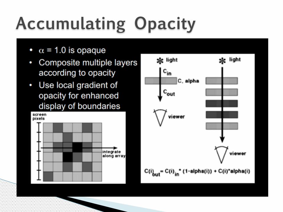
Accumulating Opacity

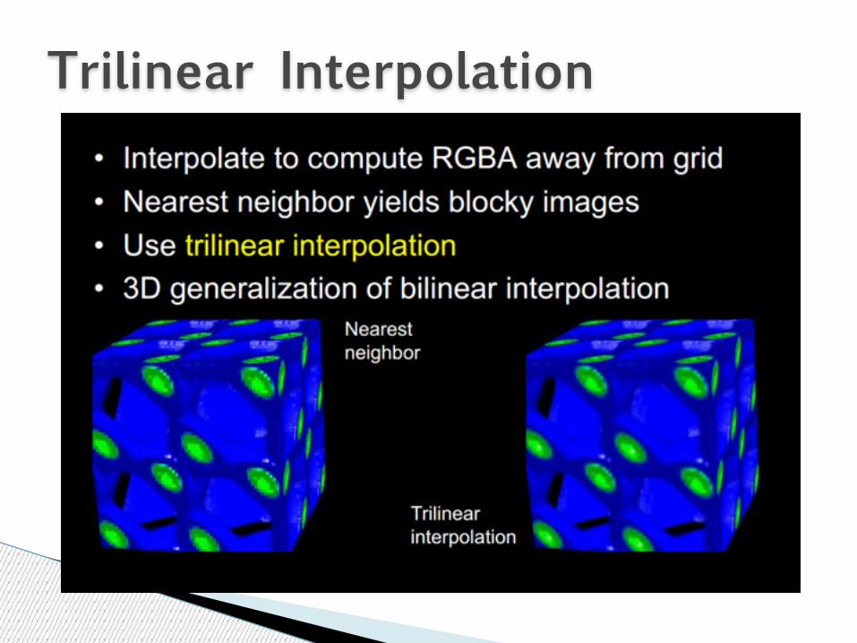
Trilinear Interpolation

Splatting

3D Textures

Example: 3D Textures

Other Techniques

! Basic problem: Huge data sets ! Must program for locality (cache) ! Divide into multiple blocks if necessary

■ example: marching cubes ! Use error measures to stop iteration ! Exploit parallelism

Acceleration of Volume Rendering

Vector Fields

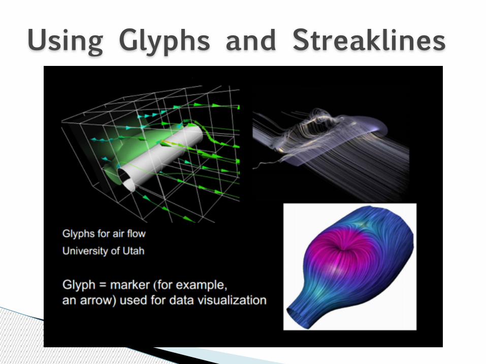
Using Glyphs and Streaklines

More Flow Examples

Example: Jet Shockwave

! Height Fields and Contours ! Scalar Fields

■ Isosurfaces ■ Marching cubes

! Volume Rendering ■ Volume ray tracing ■ Splatting ■ 3D Textures

! Vector Fields ■ Hedgehogs ■ Animated and interactive visualization

Summary

! Finite Element Models ■ general divisions of solid objects into polyhedral chunks ■ good for modeling and simulation applications

! Voxels – cube divisions, e.g. Minecraft ■ models the world with large voxels ■ takes advantage of the efficiency of local graphlike operations on voxels to model all illumination and physical dynamics as cellular finite automata

■ stores type of material in each cell (position is implicit); one byte per cubic meter of storage

! Volumetric Fog ■ constrained to fit within a containing volume

! Particle Systems

Volumetric Models

Particle Systems! What is a Particle System

! How a Particle System works

! Types of Particle Systems

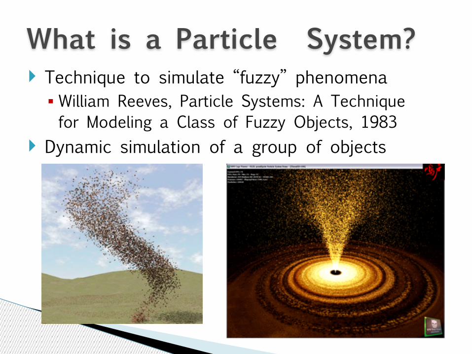
What is a Particle System?! Technique to simulate “fuzzy” phenomena

■ William Reeves, Particle Systems: A Technique for Modeling a Class of Fuzzy Objects, 1983

! Dynamic simulation of a group of objects

How a Particle System Works! Set of Points; each follow a kinematics equation ! Controlled by an Emitter ■ set of behavioral parameters and a 3D position ■ behaviors: spawning rate, initial velocity, particle life, particle

color/image ! Has two stages

1. Simulation stage 2. Rendering stage

● sprite – an image that always faces the viewer

source: Jacob Buck; maya particle system imported from Houdini with a fluidEffects shader applied

! initial position ! initial velocity (both speed and direction) ! initial size ! initial color ! initial transparency ! shape/sprite ! lifetime

Particle Attributes

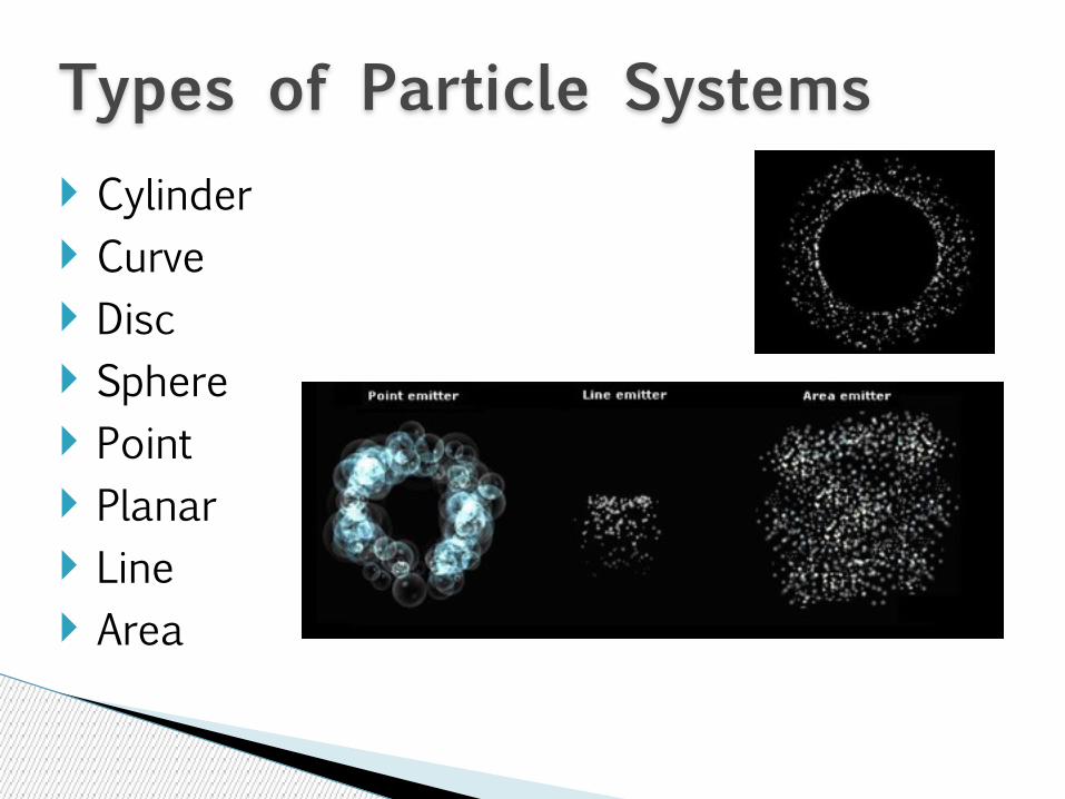
Types of Particle Systems! Cylinder ! Curve ! Disc ! Sphere ! Point ! Planar ! Line ! Area

Examples! Fire & Explosions ! Clouds & Smoke ! Water ! Falling Leaves ! Cloth ! Hair & Fur ! Galaxy

! Demo: fountain

! References: ■ http://www.opengl-tutorial.org/intermediate-tutorials/billboards-particles/particles-instancing/

■ http://www.antongerdelan.net/opengl/particles.html ■ threejs.org/examples/webgl_particles_random.html

Particle Systems in OpenGL & WebGL

http://www.opengl-tutorial.org/intermediate-tutorials/billboards-particles/particles-instancing/

http://www.antongerdelan.net/opengl/particles.html

http://threejs.org/examples/webgl_particles_random.html

Summary! Particle systems are used to create realistic natural phenomena rendering for dynamic groups of objects in real time

! Applications: ■ special effects in Animation, Games, Movies, … ■ computational science for rendering mathematical models

■ visualization

25.visualization - extra slides - Clarkson...

Documents

Transcript of 25.visualization - extra slides - Clarkson...