Master of Science in Informatics at GrenobleMaster Mathematiques Informatique - specialite Informatique

option GVR

— 2.5D Rotoscoping —A Space-Time Topological Approach

Boris DalsteinJune 21st, 2012

Research project performed at IMAGINE(joint team between Laboratoire Jean-Kuntzmann and Inria)

Under the supervision of:Dr. Remi Ronfard, Inria

Consultants:Prof. Marie-Paule Cani, Inria

Dr. Alla Sheffer, UBCEvaluated by the Thesis Committee:

Dr. Dominique AttaliProf. Nadia BraunerProf. James Crowley

Dr. Remi Ronfard

June 2012

Abstract

Rotoscoping is the task of reproducing an input video of a 3D scene with asequence of 2D drawings. It is a common task for creating special visual effects(the drawings are used as masks). It is also a commonly used technique forprofessional and amateur animators, who use video footage or even recordingsof themselves to capture subtle expressions in gestures and movements.

Rotoscoping is a difficult and tedious task, requiring a large number ofkeyframes to be drawn. One technique that could improve the efficiency ofrotoscoping is automatic inbetweening between keyframes. But this has provento be a very challenging task. The state-of-the-art in automatic inbetweeningis limited to keyframes with very little or no change in the topology of thedrawings.

In this thesis, we explore techniques for inbetweening keyframes with dif-ferent topological structures by building an explicit representation of thespace-time topology of the animation. Contrary to recent approaches, whichtackle the problem by attempting to reconstuct the depth of the 3D scene(2.5D = 2D + depth), we instead attempt to reconstruct the history of topo-logical events (2.5D = 2D + history).

The report is organized as follows: First, we review the litterature oninbetweening. Then, we present the theory of our representation for space-time topology, as well a some details of its implementation. Then, we presentan algorithm using this structure to compute automatically clean vectorialinbetweens from two drawings with inconsistent topologies. Finally, we presentsome results and discuss future work to improve them.

i

Contents

Abstract i

1 Introduction 1

2 Related Work 52.1 Early Approaches . . . . . . . . . . . . . . . . . . . . . . . . . . . . . . . 52.2 Shape Morphing . . . . . . . . . . . . . . . . . . . . . . . . . . . . . . . . 72.3 Vision-Based Approaches . . . . . . . . . . . . . . . . . . . . . . . . . . . 82.4 Using Stroke Graphs . . . . . . . . . . . . . . . . . . . . . . . . . . . . . 102.5 Restricting the Class of Animation . . . . . . . . . . . . . . . . . . . . . 13

3 Space-Time Topology 153.1 Motivations . . . . . . . . . . . . . . . . . . . . . . . . . . . . . . . . . . 153.2 Stroke Graphs As Input . . . . . . . . . . . . . . . . . . . . . . . . . . . 173.3 Animated Stroke Graph As Output . . . . . . . . . . . . . . . . . . . . . 193.4 Atomic Events . . . . . . . . . . . . . . . . . . . . . . . . . . . . . . . . . 24

4 Automatic Inbetweening 274.1 Initialisation of the algorithm . . . . . . . . . . . . . . . . . . . . . . . . 284.2 Operators: One Step of the Algorithm . . . . . . . . . . . . . . . . . . . 304.3 Deformation Energy . . . . . . . . . . . . . . . . . . . . . . . . . . . . . 324.4 Exploring the Search Space . . . . . . . . . . . . . . . . . . . . . . . . . 34

5 Experimental Results 375.1 Implementation and Interface . . . . . . . . . . . . . . . . . . . . . . . . 375.2 Results and Validation . . . . . . . . . . . . . . . . . . . . . . . . . . . . 375.3 Limitations and Future Work . . . . . . . . . . . . . . . . . . . . . . . . 43

6 Conclusion 47

Bibliography 49

iii

1 Introduction

In the past few years, there are been tremendous changes in the way people commu-nicate. “Computers” (any computing device) are more and more affordable, such thatalmost every family has one, and even almost every student of the so called developpedcountries has a “laptop”, thanks to very cheap notebooks, and the recent interest fortablets or smartphones. All of these being more and more commonly fulltime connectedthrough the Internet, virtually every person is connected permanently to any other per-son.

This revolution was such that a whole part of the Internet has been reorganizedaround social networks, mostly centered around sharing: sharing life information, sharingthoughts, sharing content. This contents is for instance images, videos or music. This isa broad new heaven for expressiveness, but unfortunately there is very few tools for –creating– this content: it is mostly created by professionals, and Internet users only shareit with their “friends”.

But we believe most people seek for creativity –eg not just sharing–, and they only lacksimple tools for that, especially in the field of animation. To fill this gap, we would liketo build an intuitive framework, for non skilled drawers or animators, to create their ownanimations. The simple idea we had to design such a tool is that creating content fromscratch needs skills by essence, while modifying existing content is much more simpler.Then, it would be intersesting to provide them proportions, timing and inspiration byusing existing videos: this is the field of rotoscoping. This technique consists in creatingan animated movie by drawing on top of a reference video, and has been first used andpatented [30] by Fleischer Max in 1917. It has been notably popularized by Walt Disney byusing it during the production of Snow White and the Seven Dwarfs in 1937. A famousreference video for rotoscoping is “The Horse in Motion” photographed by EadweardMuybridge in 1878, see Figure 1.1. Animators can redraw on top of each frame to getan animation with the right timing and poses, that will ensure an appealing motion, butpossibly with a completely new style, or even another animal.

However, even if it helps a lot compared to starting from a completely blank page,this still requires a lot of time, since every frame need to be drawn individually, with goodtime consistency. Then, this is not enough for the purpose we seek. It would be better ifthe user only draw a few representative stylized frames on top of the video (eventuallyhelped by some guidelines once he has drawn the first frame) and let the system computeall the frames inbetween.

Then, to design such an intuitive interface, we do need to tackle the difficult problemof automatic 2D inbetweening, eg given two frames of an animation at different times,compute all the intermediate frames. A lot of research on this field has been done fromthe 1970s, but despite recent advances, no general satisfactory solution has been found.Either there is a lot of restriction in the class of animation that can be drawn (and arenot robust to unaccuracy of the drawer), or it requires too much manual intervention forthe application we target.

What makes automatic inbetweening in its more general formulation really difficult

1

Figure 1.1: The Horse in Motion, photographed by Eadweard Muybridge in 1878

Figure 1.2: Three frames of a hand drawn animation, with huge topological inconsistencies

is the topological differences between the drawings, as we can see in Figure 1.2. Only apartial matching between strokes is possible (for instance the left ear is completely hiddenin the second frame), but even when a matching exists, their topological incidence canchange (for instance the jonction between the tail and the back leg: in the first framethey join at the end of the strokes, in the others the stroke of the tail ends in the middleof the stroke of the leg). If we look at the head, only a very small subset of strokes couldactually be matched all along the three frames. Then, any algorithm relying on a one-to-one correspondence would fail, and even assuming a many-to-many algorithm gives aperfect answer for strokes actually in correspondence, it doesn’t tell us much on what todo with the remaining strokes, and what to do with strokes matched to several ones.

In such a difficult case, being able to compute the right inbetweening is probablyimpossible without a human interpretation of what the drawing actually represents, andthen thanks to our knowledge of its 3D shape, draw the intermediate frames. In analgorithmic point of view, this means we need to reconstruct the 3D shape from these fewstylised representations of our object, which is a vision problem probably more complexthan our initial problem.

Due to this difficulty, so far, no existing algorithm can automatically generate inbe-tweens with topological inconsistencies, or only in very simple cases. In fact, very fewresearch as been done in this direction, directly focused on these inconsistencies. Un-fortunately, for our needs, we must handle them for three reasons: Firstly we want touse reference videos and they naturally occurs (a professional animator would design theanimation such that it doesn’t occur unless really necessary). Secondly the targeted beg-

2

giner user will make “mistakes” that a professional animator would not do, among theminacurrate drawings or not properly closed faces. Lastly the targeted user do not wantto learn a software, and then no “complicated” manipulation should be used to handlethose topological inconsistencies (a professional animator would carefully create severallayers and preform more complicated tricks).

In our case, the problem is still a bit simpler than the most general formulation: on theone hand, we can analize the reference video to help us finding the right correspondence;and on the other hand we do not require an accurate inbetweening, since our targeteduser will probably be fine with only a “not too bad” result.

The initial goal of this research was to design such an intuitive interface, where the userdraw several frames on top of a reference video, with possibly topological inconsitenciesbetween two drawings, due to the underlying 3D world (or unaccuracy of the drawer).Because the topology changes, deforming a 2D shape isn’t enough for that task: somelines should disappear, others should appear, some should split and merge together. Thisis what we call 2.5D rotoscoping.

However, we lacked a structure to describe such a 2.5D animation, where animatedlines interact with each other, by splitting or merging. Defining this structure, how tomanipulate it, how to perform computation on it, how to create inbetweens with it,and implement it appeared to be more complex than excepted, and finally the researchwas mostly focused on this part. Using the video as a mine of information to help theinbetweening algorithm has been postponed to future works.

In this report, we first review the litterature on inbetweening, where the Section 2.4defines what a stroke graph is, concept used all along our research. Then, we present thetheory about a new spatio-temporal representation of 2D animation, as well as the datastructure designed to implement this concept. Then, using this structure, we propose analgorithm to compute automatically a clean vectorial inbetweening from two drawings, inthe cases of topological inconsistencies. Starting from some initial trustful stroke corre-spondences computed automatically, the algorithm iteratively builds the whole animationby attempting to minimize an energy defined over our spatio-temporal representation. Fi-nally we present the different results of our approach, as well as what are its limitations,and discuss future work to tacke these limitations.

3

2 Related Work

The most important part of an intuitive rotoscoping system is to prevent the userto draw all the frames of a video (at 24fps for instance), since it requires so much timeand accuracy to be time consistent. The problem of inbetweening occurs when doing 2Danimation, the Walt Disney company being one of the first having to deal with it back inthe 1920s. The best reference to get in touch with traditional animation and the problemsof inbetweening is the very well-known “Illusion of Life” [48], written by two of the so-called “Nine Old Men”, heritage of Disney golden age and traditional techniques. It isalso quite known in the Computer Science community, most probably because cited bythe Lasseter’s 1987 article [25], presenting how the principles described in the book can beapplied to 3D. Of course, some others good books are also available, for instance a lot ofnice examples could be found in [8], written by Preston Blair who also worked at Disney.The book [52] also provides a mine of examples of 2D animations, the author RichardWilliams was the animation director of “Who Framed Roger Rabbit”, an animated moviebringing back a Warner-like style, instead of the Disney style of that time.

Making these inbetweens manually being tedious and time-consuming, automatic waysto do it has been looked for. In 1978, Catmull [13] provides one of the very best introduc-tion to automatic inbetweening. At that time, some attempts have been done to introducethe computer in the animation framework to help artists wherever possible, saving timeand money. For instance, Marc Levoy presents in 1977 [26] one of the first digital ani-mation systems, being developped at Cornell University. Catmull enumerates the severalpossible approaches to takle the problem of inbetweening, here are his exact words backin 1978:

1. Try to infer the missing information from the line drawings.2. Require the animators or program operators to specify the missing information by

editing.3. Break the characters into overlays.4. Use skeletal drawings.5. Use 3D outlines and centerlines.6. Restrict the class of animation that may be drawn.A detailed description of these is provided in [13]. Thirty years later, even if a lot of

progress has been done, the problem in its more general formulation can still be consideredunsolved, and it is striking to see how this enumeration is still very relevant to classifythe different papers.

2.1 Early ApproachesAs noticed in [51], many of the early approaches are stroke-based, it means they use a

“vectorial” representation of the strokes. To clarify the ideas, I mean by “vectorial” more

5

Figure 2.1: Left: a patch network (KF represent the drawn keyframes, MP the movingpoint constraints). Right: example of inbetweens generated, showing in this case contor-tion issues (image from Reeves 1981 [34])

or less any representation of curve which is not a pixelized image: it could simply be apolyline with a dense list of 2D points (eg pi+1−pi is approximatively the size of a pixel),or any explicit parameterized curves like Bezier curves. I tend not to consider as vectorialthe curves represented by implicit functions, because if we do so, pixelized images canactually be seen as a discrete sampling of an implicit function defining our curves.

One of the reason why early approaches are stroke-based is that storing complete im-ages in memory was very expensive at that time, and they did not have the computationalpower of current computers necessary to process these images (for instance, [13] explainsthat full pictures were stored for the background paintings of their animation systemat New York Institute of Technology, and that getting these pictures from the disk was“longer than desirable”). At the contrary, vectorial representations of strokes are muchmore sparse, even represented as a dense list of points, and then do not need as muchcomputational power. But I also believe the reason of this approach is that representingstrokes this way seems very natural, and is probably what anyone would think of at first,without being biased by existing recent research.

Forty-five years ago, in 1967, [31] was a first attempt at automatic inbetweening. Adeformed curve was generated by tweaking continuously its parameters via an electroniccircuit, and display the resulting curve using an analog cathode ray tube. These param-eters being still computed digitally, both analog and digital computers were used, andthen this method was presented as “hybrid curve generation”. About ten years later,considering skeletons to takle the problem of inbetweening by deforming strokes as beensuggested by Burtnyk and Wein in [12].

in 1981, Reeves in [34] proposed an approach of inbetweening using “moving pointconstraints”. The correspondences betweens strokes is given by the artist, as well as thecomplete animation path for some of them. The paths of the others is deduced by usingspace-time Coons surfaces (see Figure 2.1). This idea became commonly used in almostall computer animation systems, since it is a convenient solution, easy to implement, andthat it provides to the artist almost all the freedom he wants. For instance, a similarapproach can be used in the implementation of [51] if the artist is not pleased with theautomatic result.

Little by little, computers have replaced traditional media in almost all steps of ani-

6

mation production. In 1995, Fekete [16] presents a very good overview of their animationsystem TicTacToon, probably similar to all current animation systems. A lot of aspectsneed to be taken into account to build an efficient animation system, that computer sci-entists tend to ignore. For instance, the importance of the exposure sheet, as stated in[13], or how to handle sound syncing. The system should be convenient enough to handlehuge data management and social aspects relative to the cooperation and communicationof hundreds of people with different skills.

But as far as inbetweening is concerned, at that time not a lot of advances had beendone. For instance, it should be noted that so far, all methods required the artist tospecify a one-to-one stroke correspondence, and then that no topological changes werehandled. Then, despite the many advantages that automatic inbetweening provides, [16]claims “We have found that inputing and tuning simple in-betweens take about the sametime as drawing them by hand”.

Nevertheless, more recent works could change that statement. Indeed, not only ad-vances using stroke-based methods had been done, but also a bunch of new approacheshas emerged, notably due to the progress of Shape Morphing, Image Registration, andComputer Vision.

2.2 Shape MorphingA lot of paper dealing with “inbetweening” are in reality only dealing with the shape

morphing problem (also called shape blending). This problem is, given two closed poly-gons, how to transform the first one into the other one. Then, it only consists in smootlyblend the overall silhouette of the shape, it doesn’t address any topological change thatcan happen inside the silhouette, and what is commonly done is texture blending.

Still, shape morphing is an interesting approach, where two problems needs to besolved , exactly the same way as in inbetweening. One is the vertex correspondenceproblem (which vertex corresponds to which), the other is the vertex path problem (howto move from the first position to the second position).

If the vertex correspondence is given, a naive approach consists in a linear interpolationof the positions of the vertices, but of course, it leads to unpleasing deformations or evenself-intersection issues. In 1993, Sederberg [39] proposed an slighly better approach, usingan intrinsic definition of the polygon (each vertex of the polygon is defined locally to theprevious edge). It does not address the problem of vertex correspondence.

A solution to the vertex correspondence problem was proposed by Sebastian in 2003[38], with a method to optimally align two curves (open or closed) based on length andcurvatures. Note that this gives also a similarity metric between the two curves, thatcan actually be used to match several strokes (Remember that for the shape blendingproblem, there is only one stroke which is the silhouette).

But shape blending has mostly become popular thanks to the now very popularmethod called As-Rigid-As-Possible, proposed by Alexa et al. in 2000 [2], based on com-patible triangulations that we interpolate minimizing their local deformation. This way,the internal structure of the shape is taken into account, and provides very natural blend-ing. Note that it is only meant to solve the vertex path problem, it uses a simple user-guided approach for the vertex correspondence. It has lead to numerous improvements:in 2005, [19] adds rotation coherence constraints; in 2009, Baxter et al. [5] improved both

7

Figure 2.2: Blurring artefacts on the interior of the robot caused by any shape morphingmethod. Left: first image, Right: second image, Middle: inbetween image generated byshape morphing (image from Baxter et al. 2009 [5])

the vertex correspondence (however, a first pair of correspondence points still need tobe provided by the user) and the compatible triangulation, based on a simplified shape.The same year Baxter et al. extended it to a N-way morphing [6], to interpolate betweenmore than two shapes; and finally the automatic image registration approach proposedby Sykora et al. in 2009 [47] seems to be really promising. It has been reused for instancefor TexToons [46] that won the best paper award of the NPAR conference in 2011. Itsolves pretty nicely the vertex correspondence problem in the case of shape morphing,and does not need any manual correspondence, even if real-time dragging can be achieveif necessary.

However, whatever good the shape morphing is, it cannot handle by essence thetopological changes, and cannot be used for precise interpolation of details, notably inthe interior of the shape. Indeed, what’s happening inside of the morphed polygon is onlya texture blending between the initial textures, and then if lines are initially not at thesame position, instead of “moving”, the first one will disapear while the other one willappear, causing an unpleasing blurring effect as seen in Figure 2.2. To deal with thisproblem, Baxter and al. in 2009 [6] uses a sharper and then less noticeable blending, andFu and al. in 2005 [19] uses a streamline field over the spatial-temporal volume descibedby the morphing. However, these are only tricks that reduce slightly the visual impact,that do not at all solve the inherent problem.

Not exactly similar to shape morhping, but closed, there are all the methods to createa new shape by transforming/manipulating an existing one. For instance, As-Killing-As-Possible in 2011 [41], or the Igarashi method of 2005 using as-rigid-as-possible shapemanipulation [22]

2.3 Vision-Based ApproachesSeveral techniques can be grouped into this category, even if they are very different.

Their common point is that they use techniques mostly used by the Computer Visioncommunity, and works in the image space.

A first class of approaches are the one that aimed at separating motion from content,

8

and then apply the motion to your specific case. For instance, Bregler et al. in 2002 [10]“turns to the masters” by reusing the motion of traditional animation to retarget it toany other media. The main idea is to best approximate this motion, for each shape, usingan affine transformation and a weighted sum of key-shapes. This data is retrieved withdifferent algorithms depending on the input form of the animation (cartoon contourspoint, raw segmented video, etc...) with generally a manual intervention depending onthe animation, to segment correctly the input data (manual rotoscoping if necessary).The as rigid as possible approach is used to generate automatically plenty of other inputkey shapes, and then a Principal Component Analysis is used to select the best one andreduce the animation space. Then, they use this data to retarget the input media to anoutput animation, in different ways depending ont the excpected output. (3D shapes, 2Dshapes, etc.). This is an interesting approach, but it only helps to get the right timingof you animation. It does not hande topological changes, and it takes time to model the“output key shapes”..

An other similar paper is from De Juan and Bodenheimer in 2006 [15], which attemptsto reuse already existing 2D animation, but not only the motion: the whole animationof the character. For that, it presents a method of segmenting from videos to store thecharacters with their contour, and a method for inbetweening. The inbetweening partworks this way:

– the user manually separate the character into layers, they will be treated indepen-dently

– for each keyframe of each layer, the contour is extracted: starts at a pixel on theedge of the silhouette, and trace the contour in clockwise order

– all these points are placed in a 3D embedding, the two keyframes have differentz-values

– a 3D surface (an implicit surface generated with the points above and RBF inter-polations) is extracted with the marching cube algorithm

– The inbetween contour is the slice at the middle of this 3d surfaceIn our perspective, this paper is interesting for two main reasons: first, because it breaksthe character into several layers, it can handle some kind of topological events, this iswhat Nitzberg [32] call a 2.1D animation in 1993. However, layering is a very classicaltool provided by any decent animation software, and we want to handle are the othertypes of topological events (layering would anyway be added to the interface afterwardfor simple cases). The second reason is that it generates a Space-Time surface (definedby an implicit function in their case) to compute the inbetweens for each layer, which isin the spirit of our method (even if in practice we are really far from this approach).

Of course, when it comes to reusing existing motion, rotoscoping is a nice idea. Aninteresting method is proposed by Agarwala et al. in 2004 [1]. Guided by the user, ro-tocurves are extracted from the videos to track in time actual curves existing in the video.The, the user can draw a completely different drawing, and the stroke drawn follow thepaths of the rotocurves.

There are also “Image morphing” methods (do not confuse with shape morphing),they intend to create inbetweens of video frames. The state of the art method based onthe optical flow can generate tight inbetweens of 2 frames of a video, which is proposedby Mahajan et al. in 2009 [29]. However, it is mostly intended to be able to change theframe rate of a video, for instance by doubling it, and cannot work for our case where in

9

the one hand we have a drawing instead of a photography, and where the time distanceis way more important.

Figure 2.3: Exemple of many-to-many point correspondences (image from Yu et al. 2011[54])

Recently, in 2011, a method based on machine learning has been proposed by Yu et al.[54]. They sample the strokes into points, and for each point they compute a local shapedesciptor. Using semi-supervised learning taking into account local and global consistency[56], they are able to build a many-to-many correspondence between the sampled points,as you can see on Figure 2.3. This method has then been slighly improved in 2012 bythe same authors [53], using a different technique of learning (Graph-Based TransductiveLearning instead of Patch Alignment Framework). The main advantage to these methods(either the original or the improvement) is that it is robust, to a certain extent, totopological inconsistencies, which is what we desire in our case. However, the output of thealgorithm is not enough to compute inbetweens: the many-to-many point correspondence,even if we assume that there is no mismatch (which is generally not the case), doesn’ttell us how to interpolate the curve in those cases of topological inconsistencies.

2.4 Using Stroke GraphsThe last class of approaches, using Stroke Graphs, is by far the less explored one, while

it seems (for reasons that will be explored throughout this report) the most natural todescribe drawings as well as the most suitable to compute clean inbetweens. In order tovery fastly convince you with a non scientific argument, just consider that the state ofthe art in inbetweening is the BetweenIT system, by Whited et al. 2010 [51], researchcoming mainly from Disney Research and that has been actually used in The Princess andthe Frog, the last feature-length animation of the Walt Disney Animation Studios. Themethod using machine learning previously examined, while more recent, doesn’t provideany final result of inbetweening, but only many-to-many point correspondences. It is stillunclear how to exploit this information, but as an oracle helping another stroke matchingalgorithm.

2.4.1 DefinitionA Stroke Graph is a vectorial representation of your drawing storing the topology as

well as the geometry. To my knowledge, there are two different ways to represent it: one

10

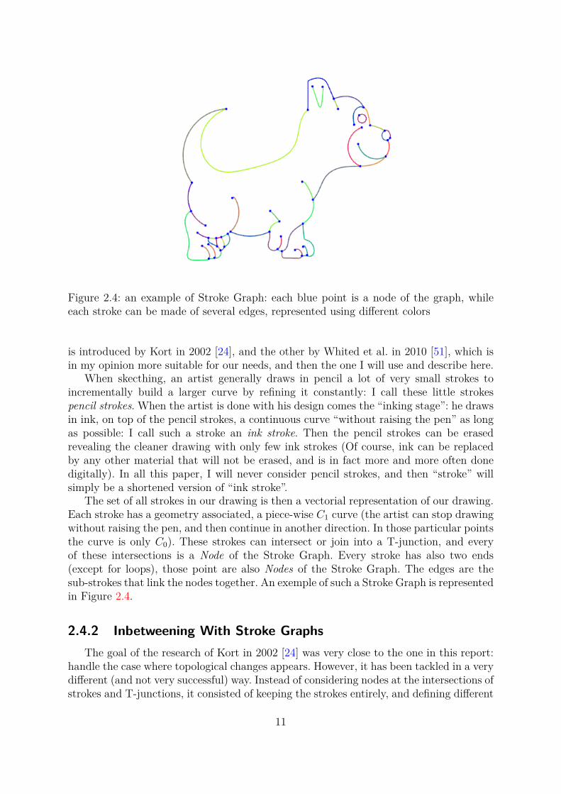
Figure 2.4: an example of Stroke Graph: each blue point is a node of the graph, whileeach stroke can be made of several edges, represented using different colors

is introduced by Kort in 2002 [24], and the other by Whited et al. in 2010 [51], which isin my opinion more suitable for our needs, and then the one I will use and describe here.

When skecthing, an artist generally draws in pencil a lot of very small strokes toincrementally build a larger curve by refining it constantly: I call these little strokespencil strokes. When the artist is done with his design comes the “inking stage”: he drawsin ink, on top of the pencil strokes, a continuous curve “without raising the pen” as longas possible: I call such a stroke an ink stroke. Then the pencil strokes can be erasedrevealing the cleaner drawing with only few ink strokes (Of course, ink can be replacedby any other material that will not be erased, and is in fact more and more often donedigitally). In all this paper, I will never consider pencil strokes, and then “stroke” willsimply be a shortened version of “ink stroke”.

The set of all strokes in our drawing is then a vectorial representation of our drawing.Each stroke has a geometry associated, a piece-wise C1 curve (the artist can stop drawingwithout raising the pen, and then continue in another direction. In those particular pointsthe curve is only C0). These strokes can intersect or join into a T-junction, and everyof these intersections is a Node of the Stroke Graph. Every stroke has also two ends(except for loops), those point are also Nodes of the Stroke Graph. The edges are thesub-strokes that link the nodes together. An exemple of such a Stroke Graph is representedin Figure 2.4.

2.4.2 Inbetweening With Stroke GraphsThe goal of the research of Kort in 2002 [24] was very close to the one in this report:

handle the case where topological changes appears. However, it has been tackled in a verydifferent (and not very successful) way. Instead of considering nodes at the intersections ofstrokes and T-junctions, it consisted of keeping the strokes entirely, and defining different

11

relations between them (for instance “intersecting” or “dangling”). Then, a series a logicalexpressions were designed in order to detect two T-junctions corresponding to the samehidden stroke, which was then reconstructed. The main advantage is the originality ofthe approach, but in fact it worked only on very simple examples.

The approach of Whited et al. in 2010 [51] is very different: what they target is“tight inbetweening”, eg inbetweening for two very close drawings. The reason comesfrom the smart observation that those tight inbetweens are the more tedious to drawmanually because of the accuracy it requires (small unaccuracy would be noticed), whileat the same time they are the simplest to compute automatically. Then, it is assumedthat the graph topology is isomorphic, or nearly isomorphic. The artist manually selectsa pair of corresponding edges in the stroke graph (or several of them) to initiate analgorithm based on graph traversal and simple edge similarity metrics, with real-timefeedback. Wherever the graph topology is the same, because strokes are very similar(tight inbetweening), this simple heuristic performs well and the algorithm matches everystroke of a connected component. The artist can run again the algorithm with other feedsto match the remaining strokes when topology has changed or when several connectedcomponents exist. The few topological changes are handled this way: if a stroke appears inonly one keyframe, the user need to manually draw the hidden line in the other keyframe,and where too much differences exist (a rotating hand is given as an example in theirpaper), the artist has the opportunity to draw himself all the inbetweens for this localdifficult part of the drawing.

Then, this method has the main advantage to reduce the artistic cost when inbe-tweens can be trustfully computed, and the artist can focus on the parts where artisticinterpretation is necessary. But a user interaction is always necessary, and it does not pro-vide an abstract representation of topological events, neither a continuous transformationwhen these topological events occur (the user needs to draw each frames manually in thiscase), neither take into account these topological events in their matching algorithm, atthe contrary of our approach.

2.4.3 About Graph IsomorphismSurprisingly, even though stroke graphs are involved, the bibliography about graph

theory doesn’t appear in inbetweening research papers. In an abstract point of view, it isclear than the problem can be formulated as belonging to the Graph Isomorphism classof problems. I present here a hierarchy of sub-classes of these problems, taken from a talkof Christine Solnon in 2009:

– Graph Isomorphism. This is an equivalence relation: “Are the graphs strictly iso-morphic?”. The complexity of this problem is called Isomorphic-complete, which isconsider rather easy in practical cases. We should notice than this is more or lessthe configuration considered by [51]

– Sub-Graph Isomorphism. This is an inclusion relation: “is this graph a strict sub-graph of that graph?”. This simple extension of the problem above is already NP-complete... but still tractable for “medium” size graphs.

– Maximum Common Subgraph. This is an intersection relation: “what are the twosugraphs of the two given graphs, which are isomorphic and maximize their size?”.Since it includes the problem above, it’s of course a NP-hard problem, and is gen-

12

erally untractable for actual application cases.– Graph Edit Distance. Find the best univalent matching (one node from first graph

matched to at most one node of the second graph) that minimizes the edition costs.it is an NP-hard problem more complicated than the previous one.

– Extended Graph Edit Distance. Find the best multivalent matching (one node fromfirst graph can be match to any number of ndoes of the second graph) that minimizesthe edition costs. NP-hard problem even more complicated than the previous one.

The first three problems are the more classical and treated in early litterature. Forinstance, with as input two graphs with weighted edges and the same number of nodes,Umeyama in 1988 [49] finds the best matching using a spectral analysis of the adjacencymatrix.

In our application case, this enumeration informs us about lots of bad news. The firstimportant one is that not only we are in the latter case (the most complicated one), butin fact the “edition” is more complex than just adding nodes and edges, popping fromnowhere. We are looking for a continuous geometric transformation from the edges of thefirst graph to the edges of the second graph. In short, we are looking for a “morphing”of strokes, not only a “matching”. In addition, aesthetics criteria should be considered:Even though it could be considered in designing an edit distance, it’s not even sure thatthe global minimum of any edit distance (assuming we could compute it) would give anappropriate result. Lastly, we would like something the user can eventually interact with,then it should be fast, possible real-time (eg far from the algorithms used in the problemsabove)

However, there is still some hope for the following reasons. First, we have a lot ofinformation attached in the stroke graph (because the edges are embedded in R2), whichnot only makes the problem simpler because the graph is planar, but in addition thegeometric information can help us in guessing the matching strokes. In addition, wewould like something the user can eventually interact with. This is indeed also goodnews: it means the user can guide the algorithm, we are not necessarily looking for fully-automatism, even if ideally it would be the goal.

The thesis of Sebastian Sorlin in 2006 [42] and the following works provides goodidea on how to solve this latter class of problems, with possibly labeled graphs whichis our case. The different approaches are using global constraints to narrow the variabledomains [43], using a reactive tabu search [44] or more recently using filtering algorithms[55, 45].

2.5 Restricting the Class of AnimationThis is not really an approach for inbetweening, but a technique to animate that

implicitly solve the problem of inbetweening, and is widely used in practice by someanimation studios. It consists, instead of drawing separate frames of the animation, inperforming 2D animation in a similar way than 3D animation: Through a dedicatedinterface (for instance ToonBoom or Adobe Flash), the artist create some vectorial 2Dobject that he will animate through time. The animation can be done either roughly bykeyframing for instance properties of the obejct such as its position and scale, but alsoby keyframing the position of the control points of the vectorial object. By using severallayers, it is possible to create complex animations.

13

However, to handle subtle topological changes, one need to carefully design the layersand use some tricks, what we would like to prevent for a begginer user. To tackle thisproblem, some research has been done in “2.5D animation”. It is important to specifythat the term is not used in the same way as the one in the title of this report. The aimof these methods is to build a model of the 2D object we want to animate using some 3Dinformation. To my knowledge, Fiore et al in 2001 [18] is the first having proposed sucha method. However, it required a lot of intervention from the user.

More recently, Rivers et al. in 2010 [35] proposed a new 2.5D model which can be moreeasily created: the user draw part of the object in different view, and then the systemautomatically compute the 3D anchor point of this 2D drawing. Then, it is possible toturn around the model: the 2D shape is interpolated in 2D, but its position is given bythe 3D position of the anchor point, which gives a nice feeling of consistent 3D, keepinga 2D style. Since it is still tedious to create those 2.5D model, An and Cai have designedin 2011 [17] a method to generate it from a 3D model.

However, if you are a casual drawer, you do not have 3D skills, and then this approachis not really adapted. Also, it can only handle the topological changes that can be solvethrough simple layering.

14

3 Space-Time Topology

3.1 MotivationsFor the reasons stated in the introduction, if one want to be able to create an intuitive

interface for 2.5D rotoscoping, an intermediate goal is to be able to generate automat-ically (or with very few intuitive user interaction) inbetweens from two drawings withtopological inconsistencies. What we call inbetweens are all the intermediate frames be-tween the two input drawings (which are called keyframes), so that the animation canbe played smoothly, for instance at a rate of 24 frames per seconds (12 frames per sec-ond is often used in traditional 2D animation to save drawing time). Two drawings arecalled topologically inconsistent when their associated stroke graphs (cf Section 2.4) arenot isomorphic 1. To clarify the ideas, the Figure 3.1 is an example of such topologicallyinconsistent stroke graphs.

?

Figure 3.1: An example of two stroke graphs with topological inconsistencies.

Now that I’ve shown this simple example which is going to be our visual supportthroughout the description of our Space-Time Topology, you are probably wondering:

1. Why should we care about automatically creating inbetweens of this?2. Does it happen in practice?

The answer to the first question is very simple: because we don’t know what the user willdraw (especially because it is a non-skilled drawer that have no idea how the interfacework), and we do want our system to be robust to any kind of input. Of course, it isimpossible to give the “perfect” inbetweens for any drawings, because sometimes suchperfect inbetweens do not exist: this is the case when even two professional inbetweenerswould draw different inbetweens for the same pair of keyframes. This happens when thereis no clear human interpretation of what the drawings represent, neither we manage tofind which strokes are in correspondence based on geometric similarities, then findingwhat’s going on between the two is problematic. But we can still define what an idealsystem should do in every cases:

– generate the good inbetweens for all sub-part of the drawings where human profes-sional inbetweeners agreed on how they should transform

1. two graphs are isomophic is there exist bijective mappings ϕ between the edges and φ between thenodes which are compatible with the relations R(n,E = {e1, ..., ek}) = “E is the set of edges incident ton” (eg R(n,E)⇔ R(φ(n), ϕ(E)))

15

Figure 3.2: Two examples of inbetweens from two different studios. Above is The Princessand the Frog from Walt Disney Animation Studios and below is Little Nemo: Adventuresin Slumberland from Tokyo Movie Shinsha. At the left is the first frame, at the rightis the last frame, and in the middle are the inbetween frames, duplicated to highlight aspecific part.

– generate inbetweens with the “lower visual impact” for the others, so that ourattention is focused on the parts correctly inbetweened

Then comes the answer to the second question: Yes, in this particular case, it doeshappen in practice, and I think professional inbetweeners would agreed on how to inbe-tween this. To demonstrate this, let’s have a look to professional animations in Figure 3.2.Parts of the drawings contains topological inconsistencies similar to the one that has beenpresented (highlighted in red). An interesting point is that the reason why these topolog-ical inconsistencies occur is different: in the first case it is line at a different depth whichbecome hidden by the arm, while in the second case it is a fold of the blanket which iscreated from an existing fold. But yet, the way it is inbetweened is similar: the new edge is“growing” from the existing edge. Then, whatever the semantic reason of the topologicalinconsistency in Figure 3.1, an automatic inbetweening system should probably generateinbetweens such as presented in Figure 3.3.

Now that we know what “should look like” the inbetweens for an input that “lookslike” the Figure 3.1, we still need to decide on our approach to tackle the problem. Thevery first question to answer is how the input and output are represented. This is themost preliminary question one can ask, but this what is all about this chapter calledSpace-Time Topology and then almost half of my Master Thesis research.

16

timetime

A

A

B

B

C

C

B

B

B

B

C

C

C

C

D

D

D

D

topologicalevent

topologicalevent

Figure 3.3: Left: how we would like the stroke graph to evolve across time. Right: Namingthe edges makes it easy to locate the two topological events, at time t1 and t2.

3.2 Stroke Graphs As InputFirst, we always have the possibility to choose between a pixelized representation of

our images or a vectorial one. They all have their pros and cons. One main advantageof vectorial representations is that they achieve easily a high quality rendering of ouranimation. Moreover, a shaky drawing with a mouse from a non professional drawer canbe more easily turned into a nice smooth vectorized curved. Then, the style of the curvecan be easily modified, it is possible to zoom in without any loss of quality, and the curvescan be easily edited by hand if necessary.

On the other hand, considering pixelized images could also be a good idea. They havethe main advantage of having more freedom: everything can be drawn, the quality onlydepends on the artist imagination, time and skills. In addition, the quite good results ofSykora et al. in 2009 [47] tends to made us think that inbetweening algorithms blendingpixels together could work: it makes them much more “flexible” especially in our case:performing a “topological operation” on a pixelized image is in fact trivial because there isno topological structure by essence, we just need to combine values of pixels for instance.

However, my belief is that a good representation for inbetweening can only be vec-torial. The first obvious advantage is that it guarantees that the rendering will be clean

17

Figure 3.4: An pair of stroke graphs containing lots of topological inconsitencies. Thedesign is taken from Catmull 1978 [13]

and similar to the input frames, without any blurring issue. The second advantage isthat the inbetweening obtained has way more useful information: not only any arbitrarynumber of frames can be generated (but it could also be the case of pixelized algorithms),but it tells you what it transformed into what. Then it can later be easily modifed, pro-cessed, slowed in or out. A typical example is coloring: the reason of the existence ofthe color transfert method Textoons [46] from Sykora in 2011 is that it is wasn’t easyto do with his inbetweening method, while the problem doesn’t exist with a vectorialalgorithm: we know exactly what are the faces all along the animation, and transferingthe coloring from one frame to all the other is trivial. Finally, I also believe that mostof the information necessary to compute a good matching between strokes (and then doa good inbetweening) is encapsulated in the topology of the stroke graph, which can becomputed only with a vectorized representation. The article from Whited at Walt DisneyAnimation Studios in 2010 [51] is mainly what makes me think so, when we see how easyit is to compute the matching by propagating good results.

For all these reasons, we choose that the input of the algorithm we are looking foris a vectorial drawing, with its 2D topology: eg the stroke graphs themselves, which arethe same input used in [51]. For instance, a simple input could be the one presentedin Figure 3.1, and a very complex input could be the pair of stroke graphs shown inFigure 3.4.

18

3.3 Animated Stroke Graph As Output

3.3.1 Abstract Data TypeNaturally, as we choosed stroke graphs for the representation of our drawing as input

of our inbetweening algorithm, it makes more sense to have an output of the same naturerather than, for instance, a sampled pixelized animation at 24 frames per seconds. Then,an abstract definition of what our output should be is a representation that can give us,for any t ∈ [0, 1], a stroke graph called StrokeGraph(t) (see Figure 3.3, left side). Butsince for every t, StrokeGraph(t) encapsulates the spatial neighbourhood information (egwhich points belong to the same edge, and which edges have a common incident node),it is also more consistent if our representation encapsulates the temporal neighbourhoodinformation. This temporal neighbourhood is which points (not necessarily at the sametime) corresponds to the same edge, and which edges are “temporally neighbours”. In thesame way as two edges are spatially neighbours is they share a common node, two edgesare said temporally neighbours if they share a common topological event. For instance, inthe Figure 3.3 (right side), we can see that A and B (as well as A and C) are temporallyneighbours. To conclude, the abstract data type 2 animated stroke graph of our outputshould provide:

– the vectorial geometry of each edge at each time– the spatial relationships between edges– the temporal relationships between edges

We will now define how this abstract data type can be represented mathematically,object combining both space-time geometry and space-time topology (see Figure 3.5), aswell as how it has been implemented.

3.3.2 Mathematical RepresentationAs for any vectorial representation of a drawing, the edges of a stroke graph are 1D

objects embedded in a 2D space: each edge E is for instance described geometrically bya parameterized curve

C : [0, 1] −→ R2

u 7−→ (x, y)If this edge is animated, then for each t in its temporal domain 3 T , its geometry isrepresented by a new curve Ct. But there is no reason to discriminate space and time inthis notation, and the geometry of our animated edge is in fact defined by

C : T × [0, 1] −→ R2

(t, u) 7−→ (x, y)

and then has been upgraded to a 2D object thanks to the time dimension. To visualize it,it is useful to embed it in the 3D space (x, y, t), that gives us a classical surface. If we do

2. From Wikipedia: an abstract data type is a mathematical model for a certain class of data structuresthat have similar behavior.

3. should be a closed connex subset of R = [−∞,+∞] (note the closed bracket), except at −∞ and+∞ where it is possibly open. For instance [−∞, t0], ] −∞, t0] and [t0, t1] are valid temporal domains,but ]t0, t1] is not valid is t0 if a finite value.

19

time

A

BC

D

t1

t2

Figure 3.5: The mathematical space-time representation (geometry and topology) of theanimation in Figure 3.3. The space-time geometry is a non-manifold 3D surface (piecewiseC1), while the space-time topology is a non-manifold 3D topological mesh, here with 4faces: A, B, C and D (If the geometry is described itself by a mesh, then the topology isa meta-mesh of the surface)

this for every animated edge of the animated stroke graph, we finally get the space-timegeometry. In the case of our example, it can be vizualized in Figure 3.5. Although this 3Dgeometric representation of a 2D animation as a surface seems really natural and adaptedfor inbetweening (the goal is to find this surface given the extremal edges), it has not beenmuch used in previous research. To my knowledge, only De Juan and Bodenheimer in2006 [15] briefly use it, defined as an implicit surface extracted using the marching cubealgorithm, and in a domain different from inbetween Buchholz et al. in 2011 [11] use itextensively to get a time-consistent parameterization of silhouettes in stylized renderingof 3D animation, given the fully pre-computed animation.

However, this recent work, even if it tracks the topological events in order to findthis time-consistent parameterization, do not have any real topological representationof the 2D animation: it only uses the space-time geometry, represented by a classicaltriangle mesh. Our approach extends this space-time geometry by including topologicalinformation to be able to use it has an animated stroke graph.

Mathematically, as can be seen in Figure 3.5, this space-time topology has the stuctureof a non-manifold 3D topological mesh, and this is all we need to represent an animatedstroke graph, since it provides everything we need:

– For any given t, StrokeGraph(t) is obtained by intersecting the space-time rep-resentation with an horizontal plane: the stroke-graph edges are where the planeinterests space-time faces, while stroke-graph nodes are where the plane intersects(non-horizontal) space-time edges.

– The topological events are represented by the space-time nodes (and the hozizontalspace-time edges).

20

A

BC

D

A

BC

D

Figure 3.6: The blue arrows represent the spatial neighbourhood relationships (left). Theright arrows represent the temporal neighbourhood relationships (right)

– Two stroke-graph edges are spatially neighbours iff their space-time face share acommon (non-horizontal) space-time edge

– Two stroke-graph edges are temporally neighbours if their space-time face share acommon space-time nodes.

We can observe that every object is downgraded by one dimension when removing thetime compononent: faces become edges, edges become nodes, and nodes (which representthe topological events) doesn’t exist anymore, as one would expected from a non-spatialobject, representing an evolution through time.

3.3.3 Data Structure

By looking at the mathematical representation described in the previous subsection,one could implement an animated stroke graph by implementing a general non-manifoldtopological data-structure, where each topological face links to its actual geometry, and itwould probably be completely fine. However, because our mathematical world is a space-time world (2D+1D) horizontal edges has a different interpretation than non horizontaledges, and it seems relevant not to describe them with the same object (eg keepingseparate spatial information and temporal information). The data structure implemented,named space-time stroke graph (STSG) is more specificly designed for our needs, and themost important aspects are presented here.

It is composed of three types of objects: edges, nodes and events. The role of edgesis to encapsulate the space-time geometry, the role of nodes is to encapsulate the spatialrelationships, while the role of events is to encapsulate the temporal relationships. Theserelashionships are represented in Figure 3.6.

21

Edges

An edge corresponds to a face of the space-time topology (Animated edge is a moreaccurate name, but it has been shortened for convenience). For instance, the animatedstroke graph represented in Figure 3.5 contains four edges: A, B, C and D. Its main roleis to contain the information about geometry, which is given by a function:

C : T × [0, 1] −→ R2

(t, u) 7−→ (x, y)Edges should be considered as not oriented. However, because it is useful for matching

to work with oriented edges, and to navigate through the graph, half-edges are defined.They are simply containing a pointer to an edge and a boolean to indicate if the orien-tation if from u = 0 to u = 1, or the opposite. They support the classical operationsnext(t), previous(t) and opposite(t) (spatial neighbourhood depends on t, cf the edge Band C of our example).

Nodes

A

BC

D

A

BC

D

E

GF

H K

Figure 3.7: The blue arrows represent the temporal relationships between the spatio-temporal edges. Spatio-temporal nodes are the objects whose role is to store those rela-tionships.

A node corresponds to the spatial relationships between edges, cf Figure 3.7: there arefive nodes named E, F, G, H, and K. At any time t, an edge has exactly two pointers tonodes: node0(t) and node1(t) (corresponding to the neighbourhood at u = 0 and u = 1).Loops are supported: in this case the two pointers are equals (pure topological loopswithout a node breaking the circle are not supported). A node contains a list of pointersto its neighbours: edges(t).

Because both edges and nodes are defined over a temporal domain T , they can beboth designed under the common terminology animated elements,

22

Events

A

B

C

D

E

GF

KH

A

C

D

E

GF

KH

Split Edge

Split Node

B

Creation

Destruction

Figure 3.8: The red arrows represents the temporal relationships between the “animatedelements” (either nodes or edges). Topological events are the objects whose role is to storethose relationships.

An event corresponds to the temporal relationships between animated elements (eitheredges and nodes), cf Figure 3.8: there are in this example four events which are namedCreation, Split Edge, Split Node and Destruction.

An event is defined by a specific finite or infinite time (the creation can appear att = −∞ for instance), as well as the list of input elements (the elements that do not existanymore after the event), and a list of input elements (the element that only exist fromthe event). Every animated element contains a pointer to its start event and its event,which always exist (but can be at infinite time). You can notice two types of duality inthis representation:

space-time duality Every edge is spatially delimited by two nodes, and equivalentlyevery animated element is temporally delimited by two events.

23

edge-node duality Split Edge is an event which transform one edge into two edgesseparated by a node, while Split Node is an event which transform one node into twonodes separated by an edge.

We have already seen that the spatial neighbourhood depends on t. In fact, the neigh-bourhood change each time a neighbour is destructed/created by an event. For instance,the neighbour of the node E is initially the edge A, but the Split Edge occurs and then itsneighbour becomes B. Then, to compute the function neighbours(t), of the node E, whatwe do is to also store a pointer to Split Edge: Split Edge is called a side event of E, andE is called a side element of Split Edge. Neighbours(startT ime) is initially given by thestart event, and then every side event informs about the changement of neighbourhood,until we arrive to the end event. This operation can be done either by chronogical order,or reverse order: the data structure is completely symmetric, every event is revertible.

3.4 Atomic EventsOur structure can allow any kind of events: an event is entirely described by:– its input elements, and a function giving for each input element what are its neigh-

bours just before the element is destructed by the event.– its output elements, and a function giving for each output element what are its

neighbours just after the element is created by the event– its side elements, and a function giving for each side elements, which of its neigh-

bours are destructed by the event, as well as which new neighbours does the elementhave after the event

With this information, all the spatial and temporal relationships of any element can beeasily retrieved when asked: there is no special need to be able to manipulate the structureto differentiate for instance SplitNode events and SplitEdge events. However, it is moreconvenient to create special classes to distinguishes the events according to their type:how many nodes/edges do they create/destruct, and what are their spatial relationships.This way, by having predifined objects for common events (such as the SplitEdge andSplitNode already seen), it is easier to operate on the structure using these predifinedevents than specifying the elements and functions presented in the list above.

Atomic events are a subset of all possible events, which are able to “simulate” anyother general event when combined, and that cannot be themselves simulated by simplerevents. Their interest is that any animation can be decribed by using only those atomicevents. Of course, the space-time topology is not the same by using two sequential eventsseparated by dt = 0, or directly the biggest event, since intermediate elements are createdin the first case, even if they have a null lifetime. However, it would be visually the samewhen played, and this is our final application.

The atomic events can be separated into two categories:– The continuous events: they create elements temporally neighbours of existing ele-

ments, and then should ensure a geometric continuity with them. This is for instancethe case of SplitNode and SplitEdge already presented.

– The non-continuous events: they create elements with no temporal neighbours: thenno geometric constraints should be met, they will appear as popping from nowhere.

24

The Figure 3.9 enumerate the list of atomic continuous events, while the Figure 3.10enumerate the list of atomic non-continuous events. If we call N− (resp E−) the numberof nodes (resp edges) in the stroke graph before the event, and N+ (resp E+) the numberof nodes (resp edges) in the stroke graph after the event, then the first column indicates(∆N,∆E) = (N+−N−, E+−E−), which highlight the duality between nodes and edgesin the terminology. An event is always invertible, and the invert of an atomic event is alsoatomic. In these tables are only listed the event in their “natural direction” (eg creatingelements), reversing the direction of the red arrow gives you the inverted atomic event.

(∆N,∆E) Name Common Cases General Case

(+0,+1) EdgeDuplicate

(+1,+1) EdgeSplit

(+1,+0) NodeDuplicate

(+1,+1) NodeSplit

Figure 3.9: The enumeration of the four continuous events.

(∆N,∆E) Name General Case

(+1,+0) NodeCreation O

(+0,+1) EdgeCreation

Figure 3.10: The enumeration of the two non-continuous events.

25

4 Automatic Inbetweening

Now that a data structure has been defined to represent an animated stroke graph,with topological events, we need to construct such an animation from two input strokegraphs to generate the inbetweening, as is presented in Figure 4.1

strokegraph 1

strokegraph 2

AutomaticInbetweening

animatedstroke graph

Figure 4.1: The input and output of our algorithm.

To achieve that, the input stroke graphs need first to be segmented. Then, they andcombined into a single trivial animated stroke graph, where all the edges from the strokegraph 1 disappear instantly, and all the edges from the stroke graph2 appear instantly.This animation is finally iteratively refined: a set of operators are generated, and we applythe one of them, depending on the strategy chosen by the algorithm. We whan have findan animation that have all its edges binded, we return this animation. This framewokcan be seen in Figure 4.2.

strokegraph 1

strokegraph 2

animatedstroke graph

segmentation

segmentation

segmentedstrokegraph 1

segmentedstrokegraph 2

combine in a trivial

animationcurrent animated

stroke graph

apply an operator

improving the animation

if the animation is OK

else

Figure 4.2: The algorithm with some little details.

27

4.1 Initialisation of the algorithm

4.1.1 Providing Input Stroke GraphsTo obtain the input stroke graph, one can:

1. directly specify them (for instance Bezier control points and tangents)2. draw on screen and fit to a vectorized line3. take as input a pixelized image and retrieve the vectorized strokesThis list is sorted in increasing order of simplicity for the user, but decreaing order

of simplicity and reliability of the algorithm. For the sake of my research, I’ve decided tochoose the second one: It is a compromize between implementation time and conveniencefor the user. Clothoids are used for the vectorial representation, which are fitted frommouse input using Ilya Baran’s own implementation of [4].

4.1.2 SegmentationBecause we want to be robust to topological changes, the first thing we need to do

is to segment the input stroke graphs. For instance, we can see in Figure 4.3 that if wedo not perform any segmentation, the first drawing is composed of three edges, while thesecond one is only composed of one drawing, and then we would have no chance to matchsome edges.

Figure 4.3: Left: without segmentation. Right: After segmentation.

For the reasons detailed by Leyton in 2006 [27], meaningful points on a shape arethe extrema of curvature, since we perceptually decompose a shape at these points. Thisapproach has also be chosen by Baxter et al. in 2009 [5] and appeared to be successful.Then, this is where we want to segment our edges. However, finding these local extremaof curvature in not trivial in the general case, since because of noise we will get a lot

28

of false positive. This way, what we look for are in fact stable extrema of curvature, amethod has been designed by [5] to compute then.

This method is far from obvious to implement, but this is where comes the choice ofclothoid curves for our vectorial representation. By definition, a clothoid spline is a curvewhose curvature is piecewise linear. Then, once the curve is fitted into a clothoid, theinformation about extrema of curvature is already encapsulated, there is no computationto do at all. The curve is given by its local minima and maxima of curvature, which arestable thanks to the good quality of the fitting. An example of segmentation is given onFigure 4.3.

4.1.3 Providing First SeedsIn the same way as [51], our algorithm first start by binding two edges together, and

then try to bind the edges of the neighbourhood of edges already binded.But then, the choice of the first binded edge is really important: we need a good

metric for that. Our approach consisted in taking into account three features of an edge:the length, the mean curvature (multiplied by the length, so that this value equals 2πfor a circle), and the diff curvature (the difference between the max of curvature and themin curvature, multiplied by the length). We know that it is a good metric, for instance,to use the ratio of the logarithms of the lengths. However, it was less clear for the meancurvature and the diff curvature. In order to know how much those features impacted onthe “difference” on two curve, we made a little perceptual study, to answer manually thequestion: “should the two edges be considered as a potential match” for different pairs ofvalues of a specific feature. The results can be seen on Figure 4.4

Figure 4.4: Green points indicates that we should consider it, red points that we shouldn’t(based on that information alone). Left: mean curvature, between −2π an pi. Right: diffcurvature, between 0 and 4π.

Based on this information, for a value x of our feature, we defined δ(x) the distancesuch that the pair (x− δ(x), x+ δ(x)) is no longer among the green points. Then, for anygiven x1 and x2, we define our metric of confidence, between 0 and 1 as:

e− dx2

2∗δ(x)2

29

where x = x1+x22 and dx = |x2 − x1|

Finally, we compute the histogram of the features among all the edges of the drawings,and divide the metric by the number of edges with similar values of this feature. This way,two edges obtain a high score not only if they are in the green area for each three features,but also if their values of features are different enough from the other. To summarize, agood score is obtained when two edges are similar, and at the same time different fromall the others.

With the features selected, which are rotation and position invariant, it improveddrastically the matching than for instance using the ratio of the features.

4.1.4 Creating the Initial AnimationThe last step of the initialization consists in creating the initial trivial animation,

which will be iteratively improved. This initial animation is simply composed of theedges from the first drawing that appear at t = −∞, then disappear at t = 0, then theedges of the second drawing appear at t = 1 and disappear at t = +∞. This animationcan be vizualized by its space-time topology in Figure 4.5.

C1

B2

B1A1

A2

time

Figure 4.5: The initial animation displayed as a space-time topology. The first drawingwas composed of the edges A1, B1 and C1, while the second drawing was composed ofthe edges A2 and B2.

4.2 Operators: One Step of the AlgorithmAt each step of our iterative algorithm, we will consider several operations that could

be done to advance one step further in the creation of the animation.

Binding a new edge If there is no already binded edges (as it is the case for the initialanimation), or if no one of the binded edges have unbinded neighbours, then the onlything we can to is binding a new edge, not connected to what has already been bindind.This operation can be seen in Figure 4.6. The potential edges considered in this case arethe best matches provided by the first seeds computation in the initialization.

30

C1

B2

B1A1

A2

A

C1

B2

B1

Figure 4.6: The result of binding a new edge. Left: before the bind. Right: after the bind

All the other three operators are used in the neighbourhood of an already bindededge.

Binding a neighbour edge This is the same operation as the previous one, except thatit happen next to an edge already binded. It is shown in Figure 4.7.

A

C1

B2

B1

A

C1

B2

B

Figure 4.7: The result of binding a neighbour edge. Left: before the bind. Right: after thebind

Making an edge grow This operator can be used to handle the case where a bindededge has a neighbour which cannot be binded. It is shown in Figure 4.8.

Spliting, then binding an edge because some topological inconsistencies need to betaken into account, it is not guaranteed (and is generally not the case), the we have thesame number of nodes along a stroke. Then, it should be possible to split an edge in two.This split is followed immediately by a bind, to ensure the algorithm is always advancing.This operator can be vizualized in Figure 4.9.

31

A

C1

B2

BA

C1

B2

BC

Figure 4.8: The result of making an edge grow. Left: before the growing. Right: after thegrowing

A

C1

B2

B1

A

C1

B2

B1

B

C2

Figure 4.9: Applying a Split and Bind. Left: before the operation. Right: after the oper-ation

Other operators should be implemented, in order to be able to represent any kind ofoperation (notably, here, no NodeDuplicate or EdgeDuplicate can be inserted) and thenbe able to create inbetweenings for a wider variety of input. However, it has not be thecase due to lack of time for this research.

It is interesting to see that from the previous exemple, we can apply an operatorBind, that gives the result on Figure 4.10. This way, both this result and the resulton Figure 4.8 are what we call a “goal animation”, eg all the edges have been binded.However, we would like to choose which one is the best. For that, we design in the nextsection an energy, and we would choose the one with a lower energy.

4.3 Deformation EnergyAs mentionned in the introduction of this chapter, our method relies on applying

iteratively the operators that has just been described. However, several choices are possibe

32

A

C1

B2

B1

B

C2

B2

B1

A B C

Figure 4.10: Result if we apply a last bind in our example.

at each step, and then in the end, the number of possible animations is really huge.What we want is to select the “best one”, in a sense that will be described in this

section: this is the one that would minimize a deformation energy defined over our struc-ture.

Because of the success of as-rigid-as-possible approaches, it seems a good idea to getinspired from them in the design of our energy. In addition, it is clear that if the seconddrawing can be exactly deduced from the first one by a rigid transform, it is probablythe one a user would expect.

A rigid transformation has the fundamental property that every distance (or equiva-lently angle) between two elements of an object is preserved all along the transformation.Let’s take t1 < t2 two different time close enough so that there is no event inbetween. Wecall G1 =StrokeGraph(t1) and G2 =StrokeGraph(t2). Our object being a stroke graph,the elements to consider are the strokes: the nodes are only here for connectivity and donot have any physical meaning, eg they have no “weight”.

Then, our physical object G1 (as well as G2) is made from infinitesimal 1D strokeelements, which have a position and a weight ds, corresponding to its infinitesimal length.Note: We could have also considered 2D surface elements for closed polygon, but sincetheir exists anyway open strokes which are only in 1D, it is hopeless (at least withoutartificial trick) to unify them in one homogeneous cost.

Consequently, for a given stroke graph G, the distances we can mesure are:

∀ds ∈ G,∀ds′ ∈ G, d(ds, ds′) = ||pos(ds)− pos(ds′)||

where “pos” is of course the position of the infinitesimal element ds. Since its length isinfinitesimal, its position is well defined (at the contrary to the complete stroke, wherewe would need to make an arbitrary choice, for instance the barycenter, or the point atmid-arclength).

Any element ds1 in G1 is continuously transformed (because there are no event inbe-tween) to an element ds2 in G2: it is given by the parameterization seen in the space-timerepresentation: In fact ds is an animated infinitesimal element of an edge, and thends1 = ds(t1) and ds2 = ds(t2). we call ds = ds1+ds2

2 the mean length between t1 and t2(we use the same notation for the infinitesimal edge and its length). Let S be the set of

33

all these infinitesimal ds . Each ds ∈ S have a starting position pos1(ds) and an endingposition pos2(ds). Then, for each (ds, ds′) ∈ S × S we can define:

d1(ds, ds′) = ||pos1(ds)− pos1(ds′)||

d2(ds, ds′) = ||pos2(ds)− pos2(ds′)||

If the transformation were rigid, we would have:

∀(ds, ds′) ∈ S × S, d1(ds, ds′) = d2(ds, ds′)

And then our cost function should look like:∫∫S×S

f(d1(ds, ds′), d2(ds, ds′)) ds ds′ where f(d, d) = 0.

We have derived the main idea of our cost function. We just need to find the rightfunction f . We figured out that using f(x, y) = (log(x)− log(y))2 works well in practice,for instance compared to f(x, y) = (x − y)2. The reason is that it lowers the impact ofdeformation from strokes far from each other.

Then, by taking t2 = t1 + dt, we have the possibility to integrate over time, betweenany two events.

4.4 Exploring the Search SpaceFinally, the only things we lack to complete this algorithm is a search strategy. In-

deed, due to the combinatorial approach, the search space grow exponentially, and it isimportant not to explore every possibility.

Greedy A naive approach consists in using a greedy algorithm. This way, we only exploreone single branch, without going back. This approach does not work at all, because thereis in almost all cases one moment were the algorithm would do a bad choice, and thenthere is no way to recover from this mistake.

Other approaches are Best-First strategies, eg based on a priority queue. For eachnew animation to explore, we attach a priority on it, and then explore it only when thispriority is the highest among the others. Depending on how we define this priority, it canhave a lot of different behaviours.

Dijkstra an interesting thing is that in the computation of our energy, we do computeonly the energy of binded edges, and then the energy is increasing little by little untilwe find a complete animation, that we excpect not having a too high energy. Since theenergy is strictly increasing, it can be interpretated as a distance in a graph, the nodesbeing the animations, and the edges the operators. Then, if we use as priority the distanceitself, we have an implementation of Dijkstra, which gives us the guarantee that the firstgoal node found (eg without unbinded edges) is actually the one with the lowest energy.However, it is generally too slow in practice.

34

Figure 4.11: Some of the 13 steps that our algorithm Closest First explores before findingthe solution on this example.

A* We can also try an implementation of A*. What we need for that is an heuristicgiving an estimated distance to a goal node. and in fact, we do have a good heuristicfor that. Indeed, if the total length of edges in the input is L, and that we have alreadybinded a length l of edges, with a current energy of E, then the energy of the goal nodeis probably close to E (L

l)2, due to the quadratic complexity of the energy. This approach

finds more often that Dijkstra a solution in a reasonable amount of time (eg less than aminute), but still doesn’t always manage to find a solution.

Closest First Then, we finally use something hybrid between a Greedy algorithm andA*. In fact, it as an A* but by using –purely– the estimated remaining distance to the goalnode, instead of the sum of the current distance plus the estimated remaining distance.This comes from the fact that the only thing we want is to find a goal node, instead offinding the shortest path to a goal node. In fact, in our search space, all paths to a nodehave the same distance, because we interpreted as distance the energy of the animation,and then does not depend on how we get there.

This last algorithm performs way better than the others. For instance, in the exampleFigure 4.11, it has found a correct solution in only 13 steps, whereas A* never managedto find a solution. Two videos showing these search behaviours are available as supple-mental material at the webpage www.dalboris.fr/masterthesis.htm. A* does exploretoo many potential combinations between “Bind” or “Split and Bind”. In the contrary,Closest First tends to keep going in the same direction since it decreases the estimatedremaining distance to the final animation. It would change its path only if the energyincreases suddenly and then compensate the fact that there is only very few edges yet tomatch. Fortunately, this is exactly what happens generally when the algorithm go into awrong path.

35

5 Experimental Results

In this section are presented the different results that have been obtained during thisMaster Thesis. Some of them are best seen with a video, those videos can be downloadedfrom the address www.dalboris.fr/masterthesis.htm.

5.1 Implementation and InterfaceMostly all the different aspects discussed in the previous sections has been imple-

mented to test our algorithms on real examples. The first step was to create an interfacefor drawing our input stroke graphs. It is really intuitive since the only possible actionis to draw with the left clic. The stroke is automatically fitted into a clothoid, the in-tersections with existing clothoids are computed, and T-junctions are cleaned. A videodemonstration of this drawing interface is available.

An important aspect of the interface is the possibility to select directly edges in orderto specify manually some correspondences, and then guide the algorithm when the fullyautomatic method does not work. Edges can also be selected by navigating using thehalf-edge data structure. A video demonstration of this is also available.

Concerning the data structure, the abstract definition of the Space-Time Stroke Graphhas been implemented, but not all the topological events, due to lack of time. This way,the only topological events we can use for now are Creation, SplitNode and SplitEdge (aswell as their inverse). The operators relative to them has been implemented, and thenit is possible to manipulate conveniently the data structure, for instance adding a Split-Edge event by applying the operators SplitEdgeAfter(t, edge) or SplitEdgeBefore(edge, t).For now, this can be done only programmatically, but it would be relatively easy withthe current interface to do it graphically, since there is already a timeline to select theappropriate time: we would just need to clic on the edge to perform the operation.

Lastly, the computation of the energy has been implemented has well as a convenientway to navigate into our search space, either manually or by applying algorithms such asGreedy, Dijkstra, A* or Closest First. By default, for all our following example here, it isClosest First which is used, unless specified differently.

5.2 Results and ValidationIn order to validate our method, we have tested it on different pairs of drawings.

Examples of succesful inbetweening are presented in Figure 5.1, 5.2 and 5.3. The videosof the animations can be downloaded at www.dalboris.fr/masterthesis.htm. In themost simple cases, no user interaction is necessary. However, in some difficult parts, theuser needs to indicate manually the good correspondence by a simple drag-and-drop.

It is important to note that in all cases that have been tested, the energy of themanually corrected solution is the lowest among all the other visited solutions. Thistends to validate the definition of our energy. For instance, the first result provided by

37

Figure 5.1: A successful result of our algorithm. The animation should be read clockwisefrom the top-left corner. One user interaction was necessary.

38

Figure 5.2: A successful result of our algorithm. The animation should be read clockwisefrom the top-left corner. No user interaction was necessary, it has been fully automaticallyinbetweened.

39

Figure 5.3: A successful result of our algorithm. The animation should be read clockwisefrom the top-left corner. Two user interactions were necessary.

40

Figure 5.4: The top row is an animation whose energy is 120, 203, while the bottom rowis an animation whose energy is 36, 734.

Figure 5.5: A naive approach to inbetween edges not automatically matched by the currentstate of art would be to make them suddenly disappearing and appearing.

the Closest First algorithm on the example Figure 5.4 was the one on the top row, whoseenergy is approximatively 120, 000. By executing Dijkstra instead, which can be donein about one second on this very simple example, we are guaranteed to find the globalminimum (restricted by our choice of operators) that can be seen on the bottom row,whose energy is around 40, 000. In general, when Closest First finds a first goal node, itis a good idea to continue the research through the remaining priority queue, in order tofind new solutions with a lower energy. On this example, the optimal solution was thethird goal node discovered, the energy were 120, 203, then 66, 380 and finally 36, 734.

A very good point of our approach is that it performs automatic inbetweening, orwith very few user interaction, in the case of topological inconsistencies and non tightinbetweens, as the contrary to the state of the art [51] which is restricted to this case. Forinstance, their algorithm would have stopped in every example in Figure 5.1, 5.2 and 5.3.whenever a topological inconsistency occurs, of if the edges are too different, which is notthe case of our method. A naive solution to handle this problem automatically would beto make suddenly appear and disappear the edges not automatically mathed. The edgesthat would not be matched automatically are presented in Figure 5.5, and a video ofthe naive solution can be downloaded, which should be compared to the video using ourapproach. Our clean interpolation of parts with topological events, even if it is a simple2D linear interpolation, induce a much stronger perception of what would be the 3Dshape.

In addition, it works exactly as well as [51] in the cases they specifically target: whenthere is no topological inconsistency. We just need to disable all operators but Bind, and

41

Figure 5.6: Segmenting two stroke graphs topologically consistent can result in two strokegraphs topologically inconsistent. Each node highlighted in red do not exist in the otherstroke graph. This example has been rotoscoped from two keyframes of The Princessand the Frog (Walt Disney Animation Studios), separated by 13 frames (at 24fps, egapproximatively half a second).

not to perform the segmentation beforehand. Then, there is only one decision at eachtime, the search space becomes linear and all our algorithms are equivalent, which makesit as efficient as [51] (in fact, probably much less because our structure is heavier, butit is equivalent in terms of number of steps). In fact, it works even better thanks to ourpremilinary pairwise likelihood: no manual interaction at all is necessary to match all thestrokes correctly in about half a second (whereas the user should give a manual seed intheir method). The reason why we can avoid user interaction is not only because we havea trustful automatic seed, but also because we have our energy, which will very quicklygrow exponentially in case of a wrong seed, and the next seed will be chosen instead,after only one or two steps.

But one can argue that in our targeted application (2.5D rotoscoping for non-skilleduser), the algorithm does not know beforehand that there is no topologocical inconsitency.Then, we cannot disable the segmentation, and this step could in fact create topologicalinconsistencies as can be seen in Figure 5.6. This happens whenever a local minimum ofcurvatures exist in only one of the two drawings. However, running our algorithm withits classical parameters perform fully automatically the good inbetweening, creating thetwo appropriate SplitEdge events. The computation took in this case four seconds in mypersonal laptop (Intel Core i7), and then is “only” height times slower than the approachof [51]. This may seem a lot, but it has to be compared to combinatorial size of the searchspace: at each step, because we can bind edges, split edges, or make them grow, with alltheir possible combinations where at T-junctions, there are about 5 possibilities at eachstep, and then all in all 5n configurations could be potentially examined (where n is maxnumber of edges, n = 61 in our example). A video of the inbetweening can be dowloaded,you can observe the two edges splitted or unsplitted at the beginning and the end of theanimation.

For a more indeep validation of the method, something that should be investigated isto ask a professional animator to draw the inbetweens for the given examples, and then

42

Figure 5.7: An example of keyframe pair that our implementation cannot inbetween yet.

compare the results to our automatic algorithm.

5.3 Limitations and Future WorkNaturally, even if it is yet very promising, there are currently a lot of limitations that

need to be tackled in the future.

5.3.1 LimitationsThe first obvious limitation is that not all topological events are implemented, and

then currently not all types of animation can be inbetweened. For instance, there is noway our current implementation can handle the input pair of drawing in Figure 5.7.Our algorithm get stuck and do not manage to converge, as can be seen in the videoavailable at www.dalboris.fr/masterthesis.htm. Typically, our approach cannot workwell in situation where layering is involved: in this case, a good approach should be firstto separate the animation into several layers, and then to use our algorithm. However,this example is interesting because no simple layering can be done (unless cutting thecharacter in two): what should be investigated is to add the concept of faces in ourapproach (can already be defined by the half-edges), and specify a depth to the edges orthe points of the face. For this reasons, Our implementation cannot currently inbetweencomplex animation such as the puppy in the introduction, or the princess from [13], sincethis kind of events occur at several places.

Another implicit limitation of this approach is that it works purely in 2D space,even if it targets topological inconsistencies which are often caused by the underlying 3Dworld. The idea behind this approach is that in 2D animation, the stylization is whatmatters most, rather than an accurate 3D consistent motion. Our definition of energywas designed so that the matching favorizes an as rigid as possible interpolation, andthen the result is probably not too far from an actual 3D motion. However, we haveyet no guarantee of this behaviour, and a counter-example can be seen in Figure 5.8,which can also be downloaded in video. This inbetweening has been obtained by running

43

Figure 5.8: An example where minimizing the energy does not give the correct 3D ex-pected behaviour.

the Dijkstra algorithm, and then is a global minimum of our energy. We can see thatthe 3D correct interpretation (a cylindric shape which is bending) is completely missed,providing instead a motion with less 2D deformations, but not adapted to this case.

Also, the combinatorial nature of the space of research is a serious limitation, since –except on simple study cases– no exhaustive search can be done to find a global minimum.Even though our Closest First approach seems a good start, I have the belief that thereexists methods drastically better. For instance, currently, the same operators are tried anexponentially number of times in a different combination when we are stuck to a barrierof energy it does not manage to pass. It seems that a better approach would be in thesecases that the algorithm tries an operation never done yet, even if at the moment itincreases too much the energy. Maybe this could be achieved by a randomized algorithm,which explores the configurations with a probability determined both by our energy, butalso depending on the number of time we have already tried that operator.

5.3.2 Future WorkThen, the most important future work should be done in the search algorithm. Having

a more precise idea on the nature of the search space is necessary, to be able to design amore adapted algorithm, with possibly proofs of convergence toward a global minimum,guarantee that we do not have using the Closest First algorithm of our approach, andthat we have using Dijkstra but whose computational time prohibits for any use in typicalinputs.

Of course, the user interface should be improved in order to have more interactionwith the inbetweening algorithm. Also, having the possibility to draw a whole animation:not only two keyframes. As an obvious improvement, it is also necessary to use anotherinterpolation between matched strokes than the current linear interpolation. Using loga-rithmic spirals as a first candidate is probably a good idea, if we refer to [51].

In addition, a lot of information could now be added to the data structure and algo-rithm to make it more task oriented. The first application we want to target is the useof a video: how the information extracted could help us to predict potential topologicalevents and anticipate them?

Finally, a generalisation of our Space-Time Topology could be done: it is probablypossible to add depth information, so that we can explain 2.1D layering event in a simplerway that actually modifying the structure to handle the event. Also, we didn’t consider atall faces in our approach, while they convey a lot of information. The reason is that facesnot always exist, and then an energy using edges seemed more natural. But inserting faces

44

in our stroke graphs seems a very good idea, since it would be intepretated as volume byadding time, and we could design an actual as rigid as possible geometric interpolation.

Finally, the “Space” component was in this research a 2D space. However, it seemsthat there is no reason it could not be extended to a 3D Space-Time Topology: eg a 4Dspace. This kind of space has already been studied by Schmid et al. in 2010 [37], becausethey he needed to track polygons in time to create stylized motion effects using shaders.

45

6 Conclusion

Vectorial automatic inbetweening in the case of topological inconsistencies was clearlyan open problem: no previous attempts have been realized successfully. However, it isnecessary to perform 2.5D rotoscoping, and then this is what has been targeted duringthis Master Thesis, focusing in developping a new approach for this problem, based onan innovative space-time approach.

The solution we proposed already works in a variety of situations, and even if it stillhas some limitations, it is a clear advance on the state of the art. In addition, it opensa lot of doors for future research, since at each step of the algorithm there are roomsfor improvements. Our solution works thanks to the combination of several contributionstogether:

– Using clothoids to perform a good segmentation.– A new statistical and perceptual method to compute the likelihood that two strokes

are in correspondence, in the context of inaccurate inbetweening.– A data structure to be able to represent the spatio-temporal topology of a vectorial

2D animation with topological events, which as never been done before.– A suitable measure of non-rigid deformation over this space-time structure.– A Best-First algorithm combining A* and Greedy ideas, well adapted to our prob-

lem.

Moreover, our data structure could be used for a wide range of applications other thaninbetweening. Of course, it can be considered for manual 2D animation, through intuitiveuser interaction. But it can also be used for multi-scale representation of an object, ifwe replace the time by the viewing distance. One could also see biological applications,to model for instance how plants are growing. To summarize, it can be used for anyapplication that needs a continuous representation of topological events.

47

Bibliography

[1] Aseem Agarwala, Aaron Hertzmann, David H. Salesin, and Steven M. Seitz.Keyframe-based tracking for rotoscoping and animation. In ACM SIGGRAPH 2004Papers, SIGGRAPH ’04, pages 584–591, New York, NY, USA, 2004. ACM.

[2] Marc Alexa, Daniel Cohen-Or, and David Levin. As-rigid-as-possible shape inter-polation. In Proceedings of the 27th annual conference on Computer graphics andinteractive techniques, SIGGRAPH ’00, pages 157–164, New York, NY, USA, 2000.ACM Press/Addison-Wesley Publishing Co.

[3] Seok-Hyung Bae, Ravin Balakrishnan, and Karan Singh. Ilovesketch: as-natural-as-possible sketching system for creating 3d curve models. In Proceedings of the 21stannual ACM symposium on User interface software and technology, UIST ’08, pages151–160, New York, NY, USA, 2008. ACM.

[4] Ilya Baran, Jaakko Lehtinen, and Jovan Popovic. Sketching clothoid splines usingshortest paths. Computer Graphics Forum, 29(2):655–664, 2010.

[5] William Baxter, Pascal Barla, and Ken-Ichi Anjyo. Compatible Embedding for 2DShape Animation. IEEE Transactions on Visualization and Computer Graphics,15(5):867–879, 2009.

[6] William Baxter, Pascal Barla, and Ken-Ichi Anjyo. N-way morphing for 2D An-imation. Computer Animation and Virtual Worlds (Proceedings of CASA), 20(2),2009.

[7] Adrien Bernhardt, Adeline Pihuit, Marie-Paule Cani, and Loıc Barthe. Matisse:Painting 2D regions for modeling free-form shapes. In Christine Alvarado and Marie-Paule Cani, editors, EUROGRAPHICS Workshop on Sketch-Based Interfaces andModeling, SBIM 2008, June, 2008, pages 57–64, Annecy, France, June 2008.

[8] P. Blair. Cartoon animation. How to Draw and Paint Series. W. Foster Pub., 1994.

[9] B. Bratt. Rotoscoping: Techniques and Tools for the Aspiring Artist. Focal Press.Focal Press, 2011.

[10] Christoph Bregler, Lorie Loeb, Erika Chuang, and Hrishi Deshpande. Turning to themasters: motion capturing cartoons. In Proceedings of the 29th annual conferenceon Computer graphics and interactive techniques, SIGGRAPH ’02, pages 399–407,New York, NY, USA, 2002. ACM.

[11] Bert Buchholz, Noura Faraj, Sylvain Paris, Elmar Eisemann, and Tamy Boubekeur.Spatio-temporal analysis for parameterizing animated lines. In Proceedings of theACM SIGGRAPH/Eurographics Symposium on Non-Photorealistic Animation andRendering, NPAR ’11, pages 85–92, New York, NY, USA, 2011. ACM.

[12] N. Burtnyk and M. Wein. Interactive skeleton techniques for enhancing motiondynamics in key frame animation. Commun. ACM, 19(10):564–569, October 1976.

49

[13] Edwin Catmull. The problems of computer-assisted animation. In Proceedings of the5th annual conference on Computer graphics and interactive techniques, SIGGRAPH’78, pages 348–353, New York, NY, USA, 1978. ACM.

[14] James Davis, Maneesh Agrawala, Erika Chuang, Zoran Popovic, and David Salesin.A sketching interface for articulated figure animation. In Proceedings of the 2003ACM SIGGRAPH/Eurographics symposium on Computer animation, SCA ’03,pages 320–328, Aire-la-Ville, Switzerland, Switzerland, 2003. Eurographics Associa-tion.

[15] Christina N. de Juan and Bobby Bodenheimer. Re-using traditional animation:methods for semi-automatic segmentation and inbetweening. In Proceedings of the2006 ACM SIGGRAPH/Eurographics symposium on Computer animation, SCA ’06,pages 223–232, Aire-la-Ville, Switzerland, Switzerland, 2006. Eurographics Associa-tion.

[16] Jean-Daniel Fekete, Erick Bizouarn, Eric Cournarie, Thierry Galas, and FredericTaillefer. Tictactoon: a paperless system for professional 2d animation. In Proceed-ings of the 22nd annual conference on Computer graphics and interactive techniques,SIGGRAPH ’95, pages 79–90, New York, NY, USA, 1995. ACM.

[17] Arcot Sowmya Fengqi An, XiongCai Cai. Automatic 2.5d cartoon modelling. IVCNZ2011, 0(0):0–0, 2011.

[18] Fabian Di Fiore, Philip Schaeken, Koen Elens, and Frank Van Reeth. Automatic in-betweening in computer assisted animation by exploiting 2.5d modelling techniques.In In Proceedings of Computer Animation (CA2001, page pages, 2001.

[19] Hongbo Fu, Chiew lan Tai, and Oscar Kin chung Au. Morphing with laplaciancoordinates and spatial-temporal texture. In Proceedings of Pacific Graphics 2005,pages 100–102, 2005.

[20] Yotam Gingold, Takeo Igarashi, and Denis Zorin. Structured annotations for 2d-to-3d modeling. In ACM SIGGRAPH Asia 2009 papers, SIGGRAPH Asia ’09, pages148:1–148:9, New York, NY, USA, 2009. ACM.

[21] Samuel Greengard. Living in a digital world. Communications of the ACM,54(10):17–19, October 2011.

[22] Takeo Igarashi, Tomer Moscovich, and John F. Hughes. As-rigid-as-possible shapemanipulation. In ACM SIGGRAPH 2005 Papers, SIGGRAPH ’05, pages 1134–1141,New York, NY, USA, 2005. ACM.

[23] J.J. Koenderink. Solid shape. Artificial intelligence. MIT Press, 1990.

[24] Alexander Kort. Computer aided inbetweening. In Proceedings of the 2nd interna-tional symposium on Non-photorealistic animation and rendering, NPAR ’02, pages125–132, New York, NY, USA, 2002. ACM.

[25] John Lasseter. Principles of traditional animation applied to 3d computer animation.In Proceedings of the 14th annual conference on Computer graphics and interactivetechniques, SIGGRAPH ’87, pages 35–44, New York, NY, USA, 1987. ACM.

50

[26] Marc Levoy. A color animation system: based on the multiplane technique. InProceedings of the 4th annual conference on Computer graphics and interactive tech-niques, SIGGRAPH ’77, pages 65–71, New York, NY, USA, 1977. ACM.

[27] M. Leyton. The Structure of Paintings. Springer, 2006.

[28] Ji Lu, Hock Soon Seah, and Feng Tian. Computer-assisted cel animation: post-processing after inbetweening. In Proceedings of the 1st international conference onComputer graphics and interactive techniques in Australasia and South East Asia,GRAPHITE ’03, pages 13–ff, New York, NY, USA, 2003. ACM.

[29] Dhruv Mahajan, Fu-Chung Huang, Wojciech Matusik, Ravi Ramamoorthi, and PeterBelhumeur. Moving gradients: A path-based method for plausible image interpola-tion. ACM Transactions on Graphics (SIGGRAPH 09), 28(3), July 2009.

[30] Fleischer Max. Method of producing moving-picture cartoons. Patent, US 1242674(A), October 1917.

[31] Takeo Miura, Junzo Iwata, and Junji Tsuda. An application of hybrid curve genera-tion: cartoon animation by electronic computers. In Proceedings of the April 18-20,1967, spring joint computer conference, AFIPS ’67 (Spring), pages 141–148, NewYork, NY, USA, 1967. ACM.

[32] M. Nitzberg, D. Mumford, and T. Shiota. Filtering, Segmentation, and Depth.Springer-Verlag New York, Inc., Secaucus, NJ, USA, 1993.

[33] G. Noris, D. Sykora, S. Coros, B. Whited, M. Simmons, A. Hornung, M. Gross, andR. W. Sumner. Temporal noise control for sketchy animation. In Proceedings of theACM SIGGRAPH/Eurographics Symposium on Non-Photorealistic Animation andRendering, NPAR ’11, pages 93–98, New York, NY, USA, 2011. ACM.

[34] William T. Reeves. Inbetweening for computer animation utilizing moving pointconstraints. In Proceedings of the 8th annual conference on Computer graphics andinteractive techniques, SIGGRAPH ’81, pages 263–269, New York, NY, USA, 1981.ACM.

[35] Alec Rivers, Takeo Igarashi, and Fredo Durand. 2.5d cartoon models. In ACMSIGGRAPH 2010 papers, SIGGRAPH ’10, pages 59:1–59:7, New York, NY, USA,2010. ACM.

[36] Damien Rohmer, Stefanie Hahmann, and Marie-Paule Cani. Exact volume preserv-ing skinning with shape control. In Symposium on Computer Animation, SCA ’09:”Moving Research”, August, 2009, pages 83–92, New Orleans, Etats-Unis, August2009. Eurographics/ACM SIGGRAPH, ACM.

[37] Johannes Schmid, Robert W. Sumner, Huw Bowles, and Markus Gross. Pro-grammable motion effects. ACM Trans. Graph., 29:57:1–57:9, July 2010.

[38] T. B. Sebastian, P. N. Klein, and B. B. Kimia. On aligning curves. IEEE Transactionson Pattern Analysis and Machine Intelligence, 25(1):116–125, 2003.

[39] Thomas W. Sederberg, Peisheng Gao, Guojin Wang, and Hong Mu. 2-d shapeblending: an intrinsic solution to the vertex path problem. In Proceedings of the 20th

51

annual conference on Computer graphics and interactive techniques, SIGGRAPH’93, pages 15–18, New York, NY, USA, 1993. ACM.

[40] Dana Sharon and Michiel van de Panne. Constellation Models for Sketch Recogni-tion. In Thomas Stahovich and Mario C. Sousa, editors, Eurographics Workshop onSketch-Based Interfaces and Modeling, pages 19–26. Eurographics Association, 2006.

[41] Justin Solomon, Mirela Ben-Chen, Adrian Butscher, and Leonidas Guibas. As-killing-as-possible vector fields for planar deformation. Computer Graphics Forum,30(5):1543–1552, 2011.

[42] Sebastien Sorlin. Mesurer la similarite de graphes. These de doctorat en infor-matique, Universite Claude Bernard Lyon I, November 2006. These encadree parChristine Solnon et Mohand-Saıd Hacid Ecole doctorale : EDIIS.

[43] Sebastien Sorlin and Christine Solnon. A global constraint for graph isomorphismproblems. In The 6th International Conference on Integration of AI and OR Tech-niques in Constraint Programming for Combinatorial Optimisation Problems ( CP-AI-OR 2004 ), Lecture Notes in Computer Science, pages 287–301. Springer Verlag,April 2004.

[44] Sebastien Sorlin and Christine Solnon. Reactive tabu search for measuring graphsimilarity. In Mario Vento Luc Brun, editor, 5th IAPR-TC-15 workshop on Graph-based Representations in Pattern Recognition, pages 172–182. Springer-Verlag, April2005.

[45] Sebastien Sorlin and Christine Solnon. A parametric filtering algorithm for the graphisomorphism problem. journal of constraints, 13(4):518–537, December 2008.

[46] Daniel Sykora, Mirela Ben-Chen, Martin Cadık, Brian Whited, and MaryannSimmons. Textoons: practical texture mapping for hand-drawn cartoon anima-tions. In Proceedings of the ACM SIGGRAPH/Eurographics Symposium on Non-Photorealistic Animation and Rendering, NPAR ’11, pages 75–84, New York, NY,USA, 2011. ACM.

[47] Daniel Sykora, John Dingliana, and Steven Collins. As-rigid-as-possible image reg-istration for hand-drawn cartoon animations. In Proceedings of International Sym-posium on Non-photorealistic Animation and Rendering, pages 25–33, 2009.

[48] F. Thomas and O. Johnston. Disney Animation: The Illusion of Life. AbbevillePress, 1987.

[49] S. Umeyama. An eigendecomposition approach to weighted graph matching prob-lems. IEEE Trans. Pattern Anal. Mach. Intell., 10(5):695–703, September 1988.

[50] Anton van den Hengel, Anthony Dick, Thorsten Thormahlen, Ben Ward, and PhilipH. S. Torr. Videotrace: rapid interactive scene modelling from video. In ACMSIGGRAPH 2007 papers, SIGGRAPH ’07, New York, NY, USA, 2007. ACM.

[51] B. Whited, G. Noris, M. Simmons, R. Sumner, M. Gross, and J. Rossignac. Be-tweenit: An interactive tool for tight inbetweening. Comput. Graphics Forum (Proc.Eurographics), 29(2):605–614, 2010.

52

[52] R. Williams. The Animator’s Survival Kit–Revised Edition: A Manual of Methods,Principles and Formulas for Classical, Computer, Games, Stop Motion and InternetAnimators. Faber and Faber, 2009.

[53] Jun Yu, Wei Bian, Mingli Song, Jun Cheng, and Dacheng Tao. Graph based trans-ductive learning for cartoon correspondence construction. Neurocomputing, 79(0):105– 114, 2012.

[54] Jun Yu, Dongquan Liu, Dacheng Tao, and Hock Soon Seah. Complex object cor-respondence construction in two-dimensional animation. Image Processing, IEEETransactions on, 20(11):3257 –3269, nov. 2011.

[55] Stephane Zampelli, Yves Deville, Christine Solnon, Sebastien Sorlin, and PierreDupont. Filtering for Subgraph Isomorphism. In 13th International Conferenceon Principles and Practice of Constraint Programming (CP’2007), LNCS, pages728–742. Springer, September 2007.

[56] Dengyong Zhou, Olivier Bousquet, Thomas Navin Lal, Jason Weston, and BernhardScholkopf. Learning with local and global consistency. In Sebastian Thrun, LawrenceSaul, and Bernhard Scholkopf, editors, Advances in Neural Information ProcessingSystems 16. MIT Press, Cambridge, MA, 2004.

53