0

2.5-D Time-Domain Finite-Difference Modelling ofTeleseismic Body Waves

Hiroshi Takenaka1 and Taro Okamoto2

1Kyushu University2Tokyo Institute of Technology

Japan

1. Introduction

Teleseismic-waveform analysis is one of the most effective approaches for study of theearthquake source process. It is also useful for investigation of the subsurface structures sincethe teleseismic seismograms have much information on the structures beneath the stations aswell as on those near source and around the paths between the source and the stations.

Analysing the teleseismic waveforms, we often calculate the synthetic seismograms. Forcomplex structures such as subduction zones, however, it may be difficult to calculate accuratesynthetic waveforms because of strong lateral heterogeneity. The laterally varying featuressuch as steep sea-bottom topography and thick sedimentary layers can have a large effect evenon long-period teleseismic body waveforms. For example, we can expect the large-amplitudelater phases as the result of the structural effect, which cannot be predicted by the flat-layeredmodel structure usually assumed in teleseismic-waveform analysis.

A full treatment of such effect requires a three-dimensional (3-D) model of the structure anda 3-D calculation for the wavefield, which requires 3-D numerical techniques such as the 3-Dfinite-difference or finite-element method. Recent advances in high performance computershave already brought full 3-D elastic modelling for seismic wave propagation within reach.Even a single CPU computer could now be used for full 3-D numerical simulations byexploitation of a single or multi-GPU (Graphics Processing Units) computing (e.g., Okamotoet al., 2010). However full 3-D modelling of large-scale seismic wave propagation is stillcomputationally expensive due to its requirements for large memory and a large number offast processors, and would be too costly even on parallel hardwares for solutions of large-sizedproblems in routine-like real data analyses because of many case computations. Nevertheless,in order to provide a quantitative analysis of real seismic records from complex regions suchas subduction zones, we need to be able to calculate the 3-D wavefields.

An economical approach to modelling of seismic wave propagation which includes manyimportant aspects of the propagation process is to examine the three-dimensional responseof a model where the material parameters vary two-dimensionally. Such a configuration inwhich a 3-D field is calculated for a 2-D medium is sometimes called two-and-a-half-dimensional(2.5-D) problem (e.g., Eskola & Hongisto, 1981). As a compromise between realism andcomputational efficiency, 2.5-D methods for calculating 3-D wavefields in 2-D varyingstructures have been developed. Bleistein (1986) developed the ray-theoretical implications of

14

www.intechopen.com

2 Will-be-set-by-IN-TECH

2.5-D modelling for acoustic problems. Luco et al. (1990) proposed a formulation for a 2.5-Dindirect boundary method using Green’s functions for a harmonic moving point force in orderto obtain the 3-D response of an infinitely long canyon, in a layered half-space, for plane elasticwaves impinging at an arbitrary angle with respect to the axis of the canyon. Pedersen et al.(1994) also presented a 2.5-D indirect boundary element method based on moving Green’sfunctions to study 3-D scattering of plane elastic waves by 2-D topographies. Takenakaet al. (1996) have developed the 2.5-D discrete wavenumber–boundary integral equationmethod, coupled with a Green’s function decomposition into P and S wave contributions,to consider the problem of the interaction of the seismic wavefield excited by a pointsource with 2-D irregular topography. Randall (1991) developed a 2.5-D velocity-stressfinite-difference technique in time domain to calculate waveforms for multipole excitation ofazimuthally nonsymmetric boreholes and formations. Okamoto (1994) also presented a 2.5-Dfinite-difference time-domain method, coupled with the reciprocal principle, to simulate theteleseismic records of a subduction earthquake. Furumura & Takenaka (1996) have developedan efficient 2.5-D formulation for the pseudospectral time-domain method for point sourceexcitation and have applied this approach successfully to modelling the waveforms recordedin a refraction survey. Such 2.5-D methods can calculate 3-D wavefields without hugecomputer memory requirements, since they require storage only slightly larger than thoseof the corresponding 2-D calculations.

In this article we consider a 2.5-D elastodynamic equation in the time domain for obliquelyincident plane waves as a means of modelling teleseismic wavefields for media with a 2-Dvariation in structure. For a 2-D medium, applying a spatial Fourier transform to the 3-Dtime-domain elastodynamic equation in the medium-constant direction along which thematerial parameters are constant, we get equations in the mixed coordinate-wavenumberdomain. These can be solved as independent sets of 2-D equations for a set ofwavenumbers. Okamoto (1994) solved the equations for each wavenumber by thestaggered-grid finite-difference time-domain method and then applied an inverse Fouriertransform over wavenumber (i.e. wavenumber summation) in order to obtain theoreticalseismograms in the spatial domain. His time-domain approach solves the source-freeelastodynamic equation in the time domain and needs to perform a large number of 2-Dcalculations. On the other hand, frequency-domain methods, such as the indirect boundarymethods mentioned above, require only one 2-D calculation for solving plane-wave incidenceproblems; they do not require wavenumber summation because in 2.5-D plane-waveincidence problems the waveslowness (medium-constant directional component) is invariant,and so at each frequency the wavenumber (medium-constant directional component) isconstant and equal to that of the incident wave. It may be related to the fact that arbitraryphase shift can easily be operated in the frequency domain while in the time domain the timeshift operation is more difficult. Takenaka & Kennett (1996a) proposed a 2.5-D “time-domain"elastodynamic equation for plane-wave incidence, which does not require wavenumbersummation. Takenaka & Okamoto (1997) then applied the staggered-grid finite-differencetechnique to this new 2.5-D equation for teleseismic body-waveform synthesis. It requirescomputation time only similar to the corresponding 2-D ones, and could reduce thecomputation time by nearly three order as compared to Okamoto (1994)’s method.

In the following sections of this article we describe the 2.5-D time-domain elastodynamicequation for plane-wave incidence and a staggered-grid finite-difference scheme for solvingthe equation, which do not require wavenumber summation, by following Takenaka &

306 Seismic Waves, Research and Analysis

www.intechopen.com

2.5-D Time-Domain Finite-Difference Modelling of Teleseismic Body Waves 3

Kennett (1996a;b) and Takenaka & Okamoto (1997). We then show two subjects ofapplications done by our group: one is an example of application to source-side structures,teleseismic waveform synthesis for source inversion; the other is an example of application toreceiver-side structures, modelling for receiver function analysis.

2. 2.5-D elastodynamic equation for a plane-wave incidence

We first use the physical properties of the wavefield to derive a 2.5-D elastodynamic equationin the time domain for the situation of an incident plane wave. Throughout this articlewe employ a Cartesian coordinate system [x, y, z], where the x and y are the horizontalcoordinates and z is the vertical one.

For an isotropic linear elastic medium, the source-free 3-D elastodynamic equation in the timedomain is given by

ρ∂ttu = ∂xτxx + ∂yτxy + ∂zτzx,

ρ∂ttv = ∂xτxy + ∂yτyy + ∂zτyz, (1)

ρ∂ttw = ∂xτzx + ∂yτyz + ∂zτzz,

where ρ = ρ(x, y, z) is the density, [u, v, w] = u = [u, v, w](x, y, z, t) are the displacements ata point (x, y, z) at time t, and the stress components are τrs = τrs(x, y, z, t), (r, s = x, y, z). Wehave used a contracted notation for derivatives ∂tt ≡ ∂2/∂t2, and ∂r ≡ ∂/∂r, (r = x, y, z). Thestress and displacement components are related by the 3-D Hooke’s law through the Laméconstants λ = λ(x, y, z) and µ = µ(x, y, z) as follows:

τxx = (λ + 2µ)∂xu + λ(∂yv + ∂zw), τyy = (λ + 2µ)∂yv + λ(∂zw + ∂xu),

τzz = (λ + 2µ)∂zw + λ(∂xu + ∂yv), τyz = µ(∂zv + ∂yw), (2)

τzx = µ(∂xw + ∂zu), τxy = µ(∂yu + ∂xv).

Numerical modelling schemes such as the finite-difference and pseudospectral methodscan compute directly discretised versions of equations (1) and (2), where the boundedcomputational domains are usually represented by grids.

We now derive a 2.5-D equation of motion for a 3-D wavefield in a 2-D medium which isconstant with respect to one coordinate and varies with the other two coordinates. We willassume the medium is constant in the y-direction throughout the rest of this article, so that thematerial properties take the form

λ = λ(x, z), µ = µ(x, z), ρ = ρ(x, z). (3)

Furthermore we assume the medium includes a homogeneous half-space underlying the 2-Dheterogeneous region whose top may be bounded by a free surface.

Consider an upgoing plane wave with horizontal slowness [px, py], which passes a point[x0, y0, z0] in the homogeneous half-space at a time t = t0. The 3-D wavefield at arbitrary timeand position in the medium including the 2-D heterogeneous region has the characteristic ofrepeating itself with a certain time delay for different observers along the medium-constantaxis (i.e., y-axis). For instance, the wavefield in the vertical plane y = y0 at the time t = t0

must be identical to that in the vertical plane y = 0 at the time t = t0 − pyy0. This means

u(x, y, x, t) = u(x, 0, z, t − pyy), τrs(x, y, x, t) = τrs(x, 0, z, t − pyy), (r, s = x, y, z). (4)

3072.5-D Time-Domain Finite-Difference Modelling of Teleseismic Body Waves

www.intechopen.com

4 Will-be-set-by-IN-TECH

If the structure is invariant in both of the horizontal (x- and y-) directions so that the materialproperties depends only on the vertical (z-) direction (i.e., 1-D heterogeneous medium),equation (4) might reduce to

u(x, y, x, t)=u(0, 0, z, t − pxx − pyy), τrs(x, y, x, t)=τrs(0, 0, z, t−pxx−pyy), (r, s= x, y, z).(5)

Note that this is ‘Snell’s law’ for plane-wave propagation in a 1-D heterogeneous medium.Equation (4) is thus a 2.5-D version of the ‘Snell’s law’ which is also mentioned below.Equation (5) could be used for modelling three-component seismic plane waves in verticallyheterogeneous media in the time domain (JafarGandomi & Takenaka, 2007; 2010; Tanaka &Takenaka, 2005).

Let us be back to the 2.5-D problem. From relations (4), the derivatives of the displacementand the stress with respect to y can be expressed as

∂yu(x, y, x, t) = −py∂tu(x, y, z, t), ∂yτrs(x, y, x, t) = −py∂tτrs(x, y, z, t), (6)

where ∂t ≡ ∂/∂t. The equivalent relations for the stress in (4) and (6) can be derived directlyfrom those for the displacement in (4) and (6) through equations (2) and (3).

Substituting (6) into (1) and (2) we obtain the equation of motion

ρ∂ttu = ∂xτxx − py∂tτxy + ∂zτzx,

ρ∂ttv = ∂xτxy − py∂tτyy + ∂zτyz, (7)

ρ∂ttw = ∂xτzx − py∂tτyz + ∂zτzz,

and the stress representations

τxx = (λ + 2µ)∂xu + λ(−py∂tv + ∂zw), τyy = −(λ + 2µ)py∂tv + λ(∂zw + ∂xu),

τzz = (λ + 2µ)∂zw + λ(∂xu − py∂tv), τyz = µ(∂zv − py∂tw), (8)

τzx = µ(∂xw + ∂zu), τxy = µ(−py∂tu + ∂xv).

This set of equations represents the 2.5-D elastodynamic response of a medium in the absenceof source. Note that all the variables in this set of equations are real-valued. When we solveequations (7) and (8), we can set y = y0, so that these equations are reduced to 2-D ones. Onceequations (7) and (8) have been solved for y = y0, we can deduce the wavefield at any y fromthat at y = y0 by shifting the time origin by py(y − y0) (see equation (4)).

We next give an alternative derivation of these time-domain 2.5-D equations (7) and(8), from the 2.5-D equations in the frequency-wavenumber domain, and recover thecharacteristic of the 2.5-D wavefield, equation (4), in the process of deriving these equations.Fourier-transforming the 3-D equations (1) and (2) with respect to t and y, we obtain thefollowing source-free 2.5-D elastodynamic equation in the frequency-wavenumber domain:

−ω2ρu = ∂x τxx − ikyτxy + ∂zτzx,

− ω2ρv = ∂x τxy − ikyτyy + ∂zτyz, (9)

−ω2ρw = ∂x τzx − ikyτyz + ∂zτzz,

308 Seismic Waves, Research and Analysis

www.intechopen.com

2.5-D Time-Domain Finite-Difference Modelling of Teleseismic Body Waves 5

and stress-displacement relations:

τxx = (λ + 2µ)∂x u + λ(−iky v + ∂zw), τyy = (λ + 2µ)(−iky)v + λ(∂zw + ∂x u),

τzz = (λ + 2µ)∂zw + λ(∂x u − iky v), τyz = µ(∂z v − ikyw), (10)

τzx = µ(∂xw + ∂zu), τxy = µ(−ikyu + ∂x v),

where we have used the y-invariance of the medium, i.e. equation (3), and have used thenotation

g(x, ky, z, ω) =1

2π

∫∞

−∞

dy e+ikyy∫

∞

−∞

dt e−iωtg(x, y, z, t), (11)

for the transform to the frequency-wavenumber domain. For a fixed value of the wavenumberky, equations (9) and (10) depend on only two space coordinates, i.e. x and z. For eachvalue of ky, these equations can therefore be solved as independent 2-D equations. Theinvariance of the medium in the y direction means that there is no coupling between differentky components. Whereas for full 3-D problems there would be coupling between differentky wavenumber components. For 2.5-D problems with an incident plane wave, we need toconsider only one ky for each ω, which is that of the incident plane wave.

The inverse transform of the double Fourier transform (11) is

g(x, y, z, t) =1

2π

∫∞

−∞

dω e+iωt∫

∞

−∞

dky e−ikyy g(x, ky, z, ω). (12)

Changing the order of the integrations, and inserting the following relation between thewavenumber ky and the slowness py:

ky = ωpy, (13)

equation (12) leads to

g(x, y, z, t) =1

2π

∫∞

−∞

dpy

∫∞

−∞

dω eiω(t−pyy)|ω|g(x, ωpy, z, ω)

=∫

∞

−∞

dpy g(x, py, z, t − pyy), (14)

where g in the time-slowness domain has been defined as

g(x, py, z, t) ≡1

2π

∫∞

−∞

dω eiωt|ω|g(x, ωpy, z, ω). (15)

We then find

1

2π

∫∞

−∞

dω eiωte−ikyy|ω|u(x, ky, z, ω) = u(x, py, z, t − pyy), (16)

and1

2π

∫∞

−∞

dωeiωte−ikyyiky|ω|u(x, ky, z, ω) = py∂tu(x, py, z, t − pyy). (17)

For an incident plane wave in a 2.5-D situation, the horizontal wavenumber ky of allwavefields is constant for each ω, and equal to that of the incident plane wave. Further from(13) we require py to be invariant and equal to the y-component of the slowness of the incident

3092.5-D Time-Domain Finite-Difference Modelling of Teleseismic Body Waves

www.intechopen.com

6 Will-be-set-by-IN-TECH

plane wave, which represents ‘Snell’s law’ for 2.5-D problems as mentioned above. Thus,when the slowness of the incident wave is py0, u(x, py, z, t − pyy) can be represented as

u(x, py, z, t − pyy) = u(x, py0, z, t − py0y) δ(py − py0), (18)

where δ(x) is the Dirac delta function. Applying the inverse transform (12) to thedisplacement in the frequency-wavenumber domain u(x, ky, z, ω), and using equations (14),(16) and (18), we obtain

u(x, y, z, t) = u(x, py0, z, t − py0y). (19)

Then,∂tu(x, y, z, t) = ∂tu(x, py0, z, t − py0y). (20)

We can recover (4) from (19) by appropriate substitutions: setting y to 0 we obtain an equationat time t and then making the particular choice t − py0y gives

u(x, 0, z, t − py0y) = u(x, py0, z, t − py0y) = u(x, y, z, t). (21)

In a similar way, we can obtain the corresponding equation for the stress. Applying the partialFourier inversions (16) and (17) to (9) and (10), and using equations (19) and (20), we recoverthe earlier forms (7) and (8).

In equations (7) and (8) the time derivatives appear on both sides of these equations, whichmay be inconvenient for direct discretisation with the finite-difference method. Here insteadof direct use of equations (7) and (8), we employ the 2.5-D equation in terms of velocity-stressthat is well suited to the use of the staggered-grid finite-difference technique. After somemanipulation of (7) and (8) (Takenaka & Kennett, 1996b), we get the following velocity-stressformulation of the 2.5-D elastodynamic equation:

∂tu = −pyρ−1β µ∂x v + ρ−1

β (∂xτxx + ∂zτzx),

∂t v = −pyρ−1α λ(∂x u + ∂zw) + ρ−1

α (∂xτxy + ∂zτyz),

∂tw = −pyρ−1β µ∂z v + ρ−1

β (∂xτzx + ∂zτzz),

∂tτxx = ν∂x u + η∂zw − pyρ−1α λ(∂xτxy + ∂zτyz),

∂tτyy = ρ−1α ρλ(∂x u + ∂zw)− pyρ−1

α (λ + 2µ)(∂xτxy + ∂zτyz), (22)

∂tτzz = η∂x u + ν∂zw − pyρ−1α λ(∂xτxy + ∂zτyz),

∂tτyz = ρ−1β ρµ∂z v − pyρ−1

β µ(∂xτzx + ∂zτzz),

∂tτzx = µ(∂xw + ∂zu),

∂tτxy = ρ−1β ρµ∂x v − pyρ−1

β µ(∂xτxx + ∂zτzx),

where [u, v, w] = [u, v, w](x, y, z, t) is the particle velocity, and

ρα ≡ ρ − p2y(λ + 2µ) = ρ(1 − α2 p2

y),

ρβ ≡ ρ − p2yµ = ρ(1 − β2 p2

y), (23)

ν ≡ (λ + 2µ) + p2yρ−1

α λ2, η ≡ λ + p2yρ−1

α λ2,

with P-wave velocity α and S-wave velocity β. When we solve (22), we can set y = 0 as wellas the case of (7) and (8) .

310 Seismic Waves, Research and Analysis

www.intechopen.com

2.5-D Time-Domain Finite-Difference Modelling of Teleseismic Body Waves 7

3. Finite-difference scheme

We use a staggered-grid finite-difference scheme (e.g., Hayashida et al., 1999; Levander, 1988;Virieux, 1986), which is stable for any values of Poisson’s ratio, making it ideal for modellingmarine problems. The finite-difference grid is staggered in time and two-dimensional space(x-z plane) as shown in Fig. 1. The y-components of particle velocity v locates at the same gridpoints as the normal stresses both in time and space. We should note the y coordinate is notdiscretised but continuous. Letting x = i∆x or x = (i ± 1/2)∆x, z = j∆z or z = (j ± 1/2)∆z,and t = l∆t or t = (l ± 1/2)∆t ; ∆x and ∆z are the grid spacings in the x- and z-direction,respectively, and ∆t is the time step, and using Levander’s notation (Levander, 1988), thedifference equations for (22) are, for example,

D+t u(i, j + 1/2, l) = ρ−1

β (i, j + 1/2)×

[−pyµ(i, j + 1/2)D−x v(i + 1/2, j + 1/2, l + 1/2)

+ D−x τxx(i + 1/2, j + 1/2, l + 1/2) + D+

z τzx(i, j, l + 1/2)],

D+t τxx(i + 1/2, j + 1/2, l + 1/2) = ν(i + 1/2, j + 1/2)D+

x u(i, j + 1/2, l + 1) (24)

+ η(i + 1/2, j + 1/2)D+z w(i + 1/2, j, l + 1)

− pyρ−1α (i + 1/2, j + 1/2)λ(i + 1/2, j + 1/2)×

[D+x τxy(i, j + 1/2, l + 1) + D+

z τyz(i + 1/2, j, l + 1)],

where D+t is forward difference operator in time, and D±

x and D±z are the forward- or

backward-difference operators in space, with sign chosen to center the difference operatorabout the quantity being updated. For example, in case of a second-order accurate in timeand fourth-order accurate in space scheme we used,

D+t u(i, j + 1/2, l) =

1

∆t[u(i, j + 1/2, l + 1)− u(i, j + 1/2, l)],

D−x v(i+1/2, j+1/2, l+1/2) =

1

∆x{c1[v(i+1/2, j+1/2, l+1/2)−v(i−1/2, j+1/2, l+1/2)]

− c2[v(i + 3/2, j + 1/2, l + 1/2)− v(i − 3/2, j + 1/2, l + 1/2)]},

D+z τzx(i, j, l + 1/2) =

1

∆z{c1[τzx(i, j + 1, l + 1/2)− τzx(i, j, l + 1/2)] (25)

− c2[ τzx(i, j + 2, l + 1/2)− τzx(i, j − 1, l + 1/2)]},

where c1 = 9/8, c2 = 1/24.

The fourth-order spatial finite-difference scheme usually needs more than five grid points perwavelength (Levander, 1988). The finite-difference region (computational domain) is dividedinto two parts: a model zone for the upper part and an initial wave zone for the lower part. Themodel zone fully includes the target structural model and may be heterogeneous. The initialwave zone locates under the model zone and should be homogeneous. It is needed for theincident wave, and an upgoing plane wave is input as the initial condition within it. Theinitial wave zone should have no velocity contrast at the interface contacting the model zone

3112.5-D Time-Domain Finite-Difference Modelling of Teleseismic Body Waves

www.intechopen.com

8 Will-be-set-by-IN-TECH

to prevent artificial reflections and conversions. The size of the computational domain is setsufficiently large so that artificial noises, such as noises from the both ends of the input planewave, can be ignored. As Okamoto (1994) we here select the time step as 62 % of the maximumallowed time step by the stability condition for the 2-D P − SV finite-difference scheme of asecond-order accurate in time and fourth-order accurate in space (Levander, 1988).

v, τxx, τyy, τzz, τzxt

u, w, τxy, τyz

t∆

(a) Temporal grid.

v, τxx, τyy, τzzx

u, τxy

w, τyz

τzx∆

∆

z

x

z

(b) Spatial grid.

Fig. 1. Discretisation of (a) time and (b) space.

4. Teleseismic waveform synthesis for source inversion

Seismic displacement due to a point source of earthquake may be expressed as

un(x, t) = Mpq(t) ∗ ∂qGn;p(x, t; ξ, 0), (26)

where Mpq(t) is moment tensor with time varying components, operation ∗ is convolutionwith respect to time t, and Gn;p(x, t; ξ, τ) is displacement Green’s tensor representing the nthcomponent of elastic displacement at a receiver position x and time t caused by a unit pointforce in the p-direction at a source position ξ and time τ (e.g., Aki & Richards, 2002). We haveused the convention of summation over repeated suffices. In source inversions derivative ofthe GreenAfs tensor ∂qGn;p(x, t; ξ, 0) is empirically called just “Green’s function". We herefollow this custom.

Applying the spatial reciprocity:

Gn;p(x, t; ξ, 0) = Gp;n(ξ, t; x, 0), (27)

equation (26) reduces to

un(x, t) = Mpq(t) ∗ ∂qGp;n(ξ, t; x, 0)

= Mpq(t) ∗ Epq;n(ξ, t; x, 0), (28)

where Epq;n(ξ, t; x, 0) is the strain tensor at the source position corresponding to Gp;n(ξ, t; x, 0).This equation shows as follows. The reciprocity of the elastodynamic theory is exploited

312 Seismic Waves, Research and Analysis

www.intechopen.com

2.5-D Time-Domain Finite-Difference Modelling of Teleseismic Body Waves 9

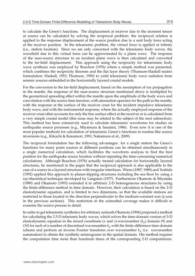
to calculate the Green’s functions. The displacement at receiver due to the moment tensorat source can be calculated by solving the reciprocal problem; the reciprocal relation isapplied to the response displacement at the source position due to a unit body force actingat the receiver position. In the teleseismic problem, the virtual force is applied at infinity(i.e., station location). Since we are only concerned with the teleseismic body waves, thewavefield due to this virtual force can be approximated by a plane wave. The responseof the near-source structure to an incident plane wave is then calculated and convertedto the far-field displacement. This approach using the reciprocity for teleseisimic bodywave synthesis was employed by Bouchon (1976) where a simple method was presented,which combines the reciprocity theorem and the flat layer theory (Thomson-Haskell matrixformulation: Haskell, 1953; Thomson, 1950) to yield teleseismic body wave radiation fromseismic sources embedded in the horizontally layered crustal models.

For the conversion to the far-field displacement, based on the assumption of ray propagationin the mantle, the response of the near-source structure mentioned above is multiplied bythe geometrical spreading effect within the mantle upon the amplitude of the body wave andconvolution with the source time function, with atenuation operator for the path in the mantle,with the response at the surface of the receiver crust for the incident impulsive teleseismicbody wave, and with the instrumental response, where the actually employed response of thereceiver crust often accounts for only the free surface effect at the receiver or is calculated froma very simple crustal model (this issue may be related to the subject of the next subsection).This method has been extensively used to calculate teleseismic waveforms for studies onearthquake source processes (e.g., Miyamura & Sasatani, 1986). Even now it is one of themost popular methods for calculation of teleseismic Green’s functions in routine-like sourceinversions (e.g., Kikuchi & Kanamori, 1991; Nakamura et al., 2009).

The reciprocal formulation has the following advantages: for a single station the Green’sfunctions for many point sources at different positions can be obtained simultaneously ina single numerical calculation, which facilitates the waveform analysis to find the bestposition for the earthquake source location without repeating the time-consuming numericalcalculations. Although Bouchon (1976) actually treated calculation for horizontally layeredstructures, he mentioned in the paper that the reciprocal approach is also applicable to thecase of a source in a layered structure with irregular interfaces. Wiens (1987; 1989) and Yoshida(1992) applied this approach to planar-dipping structures including the sea floor by using aray-theoretical technique developed by Langston (1977). Furthermore Okamoto & Miyatake(1989) and Okamoto (1993) extended it to arbitrary 2-D heterogeneous structures by usingthe finite-difference method in time domain. However, their calculation is based on the 2-Delastodynamic equation, and is limited to two dimenions, so that the available stations arerestricted to those located in the direction perpendicular to the medium-constant axis (y-axisin the previous sections). This restriction in the azimuthal coverage makes it difficult toexamine the source process in detail.

In order to get teleseismic synthetics for arbitrary azimuth Okamoto (1994) proposed a methodfor calculating the 2.5-D telseismic body waves, which solves the time-domain version of 3-Delastodynamic equation in the mixed coordinate (x and z)-wavenumber (ky) domain (9) and(10) for each of a number of discretised wavenumber ky with the finite-difference time-domainscheme and perform an inverse Fourier transform over wavenumber ky (i.e. wavenumbersummation) to obtain the synthetic seismograms in the spatial domain. His method requiresthe computation time more than hundreds times of the corresponding 2-D computations.

3132.5-D Time-Domain Finite-Difference Modelling of Teleseismic Body Waves

www.intechopen.com

10 Will-be-set-by-IN-TECH

Takenaka et al. (1997) presented a method without wavenumber summation so that 2.5-Dteleseismic synthetics requires only computation time similar to the corresponding 2-D ones.This method uses the 2.5-D elastodynamic equation for a plane-wave incidence (22) and itsfinite-difference time-domain scheme proposed by Takenaka & Okamoto (1997) which wasdescribed in the previous section. It has been employed for calculating teleseismic Green’sfunctions in several source inversion studies (e.g., Okamoto & Takenaka, 2009a;b) and formodelling the teleseismic waveforms including a near-source scattering inside a subductedplate (Kaneshima et al., 2007). We here show two results for source inversion among them asexamples.

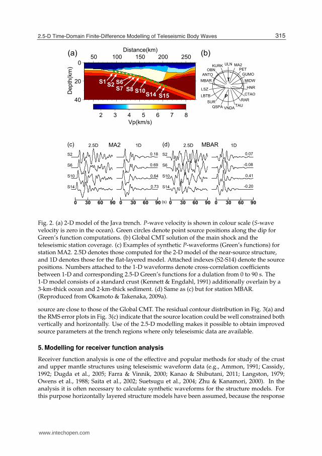
Figure 2 shows comparison of the teleseismic Green’s function waveforms from the 2-Dmodel with those from 1-D (flat-layered) models for a source inversion of the 17-July-2006Java tsunami earthquake (MW7.8 by Okamoto & Takenaka, 2009a, USGS PDE: 08:19:26.6,9.284◦S, 107.419◦E, depth 20 km, http://earthquake.usgs.gov/research/data). The materialproperties of the assumed Java trench model (Fig. 2(a)) are allowed to vary with respectto the trench-perpendicular axis, while they are assumed to be invariant with respect to thetrench-parallel axis. This model was constructed from the results of seismic surveys in thenearby area (Kopp et al., 2002) and global reference models (Dziewonski & Anderson, 1981;Kennett & Engdahl, 1991; Laske et al., 2001). In Fig. 2(a) the point sources for Green’s functioncomputations are located along the dip of the main-shock fault plane. The along-dip intervalof source points is 8.0 km for the section from S1 to S8 and 8.1 km for the section from S8to S15. The rigidity for sources S1-S7 is 16.3 GPa and for sources S8-S15, 38.6 GPa. The bestdouble couple of the Global CMT solution (http://www.globalcmt.org) shown in Fig. 2(b) isemployed for each Green’s function computation. Following the standard 1-D teleseismicwave computations, mantle attenuation is incorporated by choosing t∗ = 1.0 for P-wavesand 4.0 for SH-waves, while anelastic attenuation is not included in the finite-differencecomputations that evaluate near-source response. The 1-D Green’s functions were computedby the method of Kroeger & Geller (1983). The comparison between waveforms of the2.5-D and flat-layered Green’s functions (Fig. 2(c)) clearly illustrates the large effect of theheterogeneous structure on the body waves. The waveforms of 2.5-D Green’s functions haveprolonged, large amplitude later phases. They appear irrespective of station azimuth, andare not reproduced by 1-D model. At the oceanic trench regions large effect of laterallyheterogeneous structure is expected to appear on the teleseismic body waveforms: thickwater layer, dipping ocean bottom, and thick sediments near the source distort ray pathsto teleseismic stations and often cause large later phases on the teleseismic body waveforms.This effect must be evaluated carefully before a detailed source process analysis is applied toreal earthquake records.

Okamoto & Takenaka (2009b) studied strong effect of near-source structure on teleseismicbody waveforms from two well-recorded aftershocks of the 2006 Java tsunami earthquake.Figure 3 shows the results of one of the two events: MW6.1, 2006/07/17 15:45:59.8, 9.420◦S108.319◦E. They applied a “waveform relocation technique" which combines a waveforminversion of source parameters with a grid search procedure to correct possible systematic biasin hypocentral parameters. In the waveform inversion 2.5-D teleseismic Green’s functionsare used. The grid spacing for grid search is 2 km horizontally and 1 km vertically. In Fig.3(b), the 2.5-D synthetic seismograms are compared with the observation records. In mostof the stations, peaks and troughs in the observed later arrivals are well reproduced by thesynthetics. The best position (Fig. 3(a), (c)) and the mechanism (Fig. 3(b)) of the obtained point

314 Seismic Waves, Research and Analysis

www.intechopen.com

2.5-D Time-Domain Finite-Difference Modelling of Teleseismic Body Waves 11

0

20

40

Depth

(km

)

50 100 150 200 250

Distance(km)

2 3 4 5 6 7 8

Vp(km/s)

(a)

S2 S6

S10S14

S1

S8S7

S15

T

P

ULN MA2PET

GUMO

MIDW

HNR

CTAO

RAR

TAUVNDAQSPA

SUR

LBTB

LSZ

MBAR

ANTO

OBNKURK

(b)

S2

S6

S10

S14

2.5D 1D(c) MA2 2.5D 1D(d) MBAR

0 30 60 90 0 30 60 90 0 30 60 90 0 30 60 90

S2

S6

S10

S14

(s)

0.18

0.69

0.64

0.73

0.07

-0.08

0.41

-0.20

Fig. 2. (a) 2-D model of the Java trench. P-wave velocity is shown in colour scale (S-wavevelocity is zero in the ocean). Green circles denote point source positions along the dip forGreen’s function computations. (b) Global CMT solution of the main shock and theteleseismic station coverage. (c) Examples of synthetic P-waveforms (Green’s functions) forstation MA2. 2.5D denotes those computed for the 2-D model of the near-source structure,and 1D denotes those for the flat-layered model. Attached indexes (S2-S14) denote the sourcepositions. Numbers attached to the 1-D waveforms denote cross-correlation coefficientsbetween 1-D and corresponding 2.5-D Green’s functions for a dulation from 0 to 90 s. The1-D model consists of a standard crust (Kennett & Engdahl, 1991) additionally overlain by a3-km-thick ocean and 2-km-thick sediment. (d) Same as (c) but for station MBAR.(Reproduced from Okamoto & Takenaka, 2009a).

source are close to those of the Global CMT. The residual contour distribution in Fig. 3(a) andthe RMS error plots in Fig. 3(c) indicate that the source location could be well constrained bothvertically and horizontally. Use of the 2.5-D modelling makes it possible to obtain improvedsource parameters at the trench regions where only teleseismic data are available.

5. Modelling for receiver function analysis

Receiver function analysis is one of the effective and popular methods for study of the crustand upper mantle structures using teleseismic waveform data (e.g., Ammon, 1991; Cassidy,1992; Dugda et al., 2005; Farra & Vinnik, 2000; Kanao & Shibutani, 2011; Langston, 1979;Owens et al., 1988; Saita et al., 2002; Suetsugu et al., 2004; Zhu & Kanamori, 2000). In theanalysis it is often necessary to calculate synthetic waveforms for the structure models. Forthis purpose horizontally layered structure models have been assumed, because the response

3152.5-D Time-Domain Finite-Difference Modelling of Teleseismic Body Waves

www.intechopen.com

12 Will-be-set-by-IN-TECH

��������

����

����

�� ������

������ ������

������������

����

���

���

����

����

�����

�����

����

T

P

MA2

PET

GUMO

HNR

VNDASUR

LBTB

LSZ

MBAR

OBN

KURKULN

MA2 P

DATA

4.4

SYN

PET P 4.6

GUMO P 4.7

HNR P 3.9

VNDA P 3.0

SUR P 4.0

LBTB P 3.0

LSZ P 2.6

MBAR P 1.7

OBN P 4.0

KURK P 5.5

ULN P 5.8

VNDA SH 2.8

LBTB SH 9.7

KURK SH 7.3

0 35 70Time(s)

STF

X= 140.0km DEPTH= 13.0km RESIDUAL= 0.550(b)

(C)

RM

S E

rror

(s)

1.32

1.36

1.40

1.44

1.48

-20 -10 0 10

Trench Parallel Distance (km)

2.5D

Fig. 3. (a) Open star indicates the best point source position of the 17-July-2006 event(MW6.1). Locations of Global CMT (triangle) and PDE (diamond) are also projected. Thecontour lines denote the residual distribution of the grid search relocation by the waveforminversion. The contour interval is 0.02. (b) Observed (top) and 2.5-D synthetic (bottom)waveforms. Attached number denotes the maximum amplitude of the observed waveformin µm. Also plotted are the source time function (STF) and the focal mechanism. A timewindow of 70 s after the onset (indicated by vertical lines) is used for the inversion. Theestimated moment tensor components in unit of 1017 Nm are: Mrr = −1.81, Mθθ = 4.63,Mφφ = −2.81, Mrθ = 11.1, Mrφ = −2.04, Mθφ = 0.67, which yield a scalar moment of

1.19 × 1018 Nm (MW6.0). (c) RMS error in travel time analysis plotted versus the distancewith respect to trench-parallel axis (positive toward N116◦E with the origin placed on thecross section through the PDE epicenter). Most of the travel times listed in USGS NEICMonthly Earthquake Data Report are used. (Reproduced from "Effect of near-source trenchstructure on teleseismic body waveforms: an application of a 2.5D FDM to the Java trench"by T. Okamoto & H. Takenaka, in Advances in Geosciences, Vol. 13 (Solid Earth), Ed. KenjiSatake, Copyright (C) 2009 by World Scientific Publishing.)

316 Seismic Waves, Research and Analysis

www.intechopen.com

2.5-D Time-Domain Finite-Difference Modelling of Teleseismic Body Waves 13

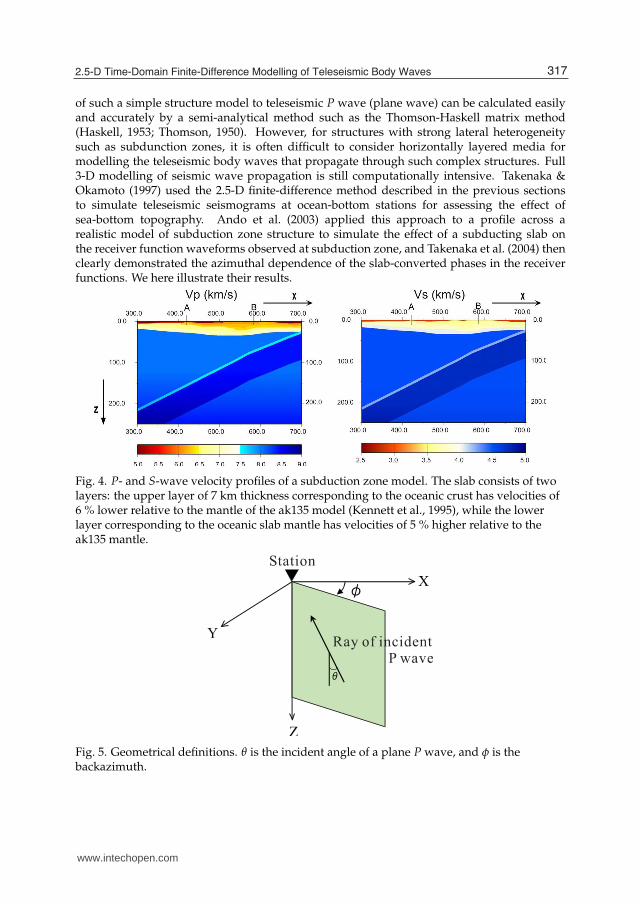
of such a simple structure model to teleseismic P wave (plane wave) can be calculated easilyand accurately by a semi-analytical method such as the Thomson-Haskell matrix method(Haskell, 1953; Thomson, 1950). However, for structures with strong lateral heterogeneitysuch as subdunction zones, it is often difficult to consider horizontally layered media formodelling the teleseismic body waves that propagate through such complex structures. Full3-D modelling of seismic wave propagation is still computationally intensive. Takenaka &Okamoto (1997) used the 2.5-D finite-difference method described in the previous sectionsto simulate teleseismic seismograms at ocean-bottom stations for assessing the effect ofsea-bottom topography. Ando et al. (2003) applied this approach to a profile across arealistic model of subduction zone structure to simulate the effect of a subducting slab onthe receiver function waveforms observed at subduction zone, and Takenaka et al. (2004) thenclearly demonstrated the azimuthal dependence of the slab-converted phases in the receiverfunctions. We here illustrate their results.

Fig. 4. P- and S-wave velocity profiles of a subduction zone model. The slab consists of twolayers: the upper layer of 7 km thickness corresponding to the oceanic crust has velocities of6 % lower relative to the mantle of the ak135 model (Kennett et al., 1995), while the lowerlayer corresponding to the oceanic slab mantle has velocities of 5 % higher relative to theak135 mantle.

Fig. 5. Geometrical definitions. θ is the incident angle of a plane P wave, and φ is thebackazimuth.

3172.5-D Time-Domain Finite-Difference Modelling of Teleseismic Body Waves

www.intechopen.com

14 Will-be-set-by-IN-TECH

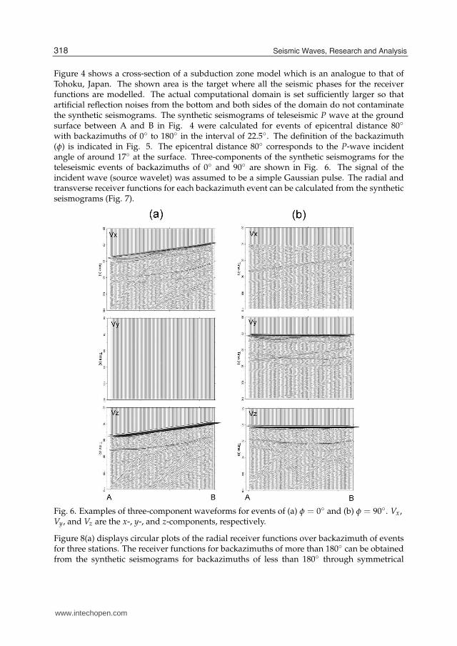
Figure 4 shows a cross-section of a subduction zone model which is an analogue to that ofTohoku, Japan. The shown area is the target where all the seismic phases for the receiverfunctions are modelled. The actual computational domain is set sufficiently larger so thatartificial reflection noises from the bottom and both sides of the domain do not contaminatethe synthetic seismograms. The synthetic seismograms of teleseismic P wave at the groundsurface between A and B in Fig. 4 were calculated for events of epicentral distance 80◦

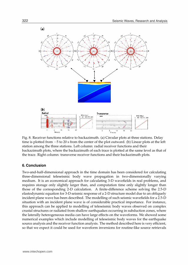
with backazimuths of 0◦ to 180◦ in the interval of 22.5◦. The definition of the backazimuth(φ) is indicated in Fig. 5. The epicentral distance 80◦ corresponds to the P-wave incidentangle of around 17◦ at the surface. Three-components of the synthetic seismograms for theteleseismic events of backazimuths of 0◦ and 90◦ are shown in Fig. 6. The signal of theincident wave (source wavelet) was assumed to be a simple Gaussian pulse. The radial andtransverse receiver functions for each backazimuth event can be calculated from the syntheticseismograms (Fig. 7).

Fig. 6. Examples of three-component waveforms for events of (a) φ = 0◦ and (b) φ = 90◦. Vx,Vy, and Vz are the x-, y-, and z-components, respectively.

Figure 8(a) displays circular plots of the radial receiver functions over backazimuth of eventsfor three stations. The receiver functions for backazimuths of more than 180◦ can be obtainedfrom the synthetic seismograms for backazimuths of less than 180◦ through symmetrical

318 Seismic Waves, Research and Analysis

www.intechopen.com

2.5-D Time-Domain Finite-Difference Modelling of Teleseismic Body Waves 15

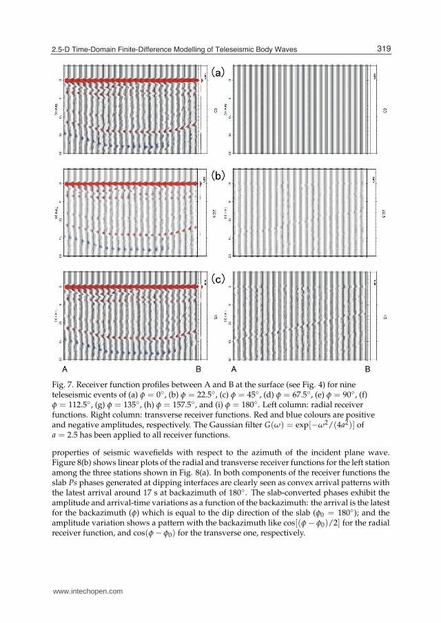
Fig. 7. Receiver function profiles between A and B at the surface (see Fig. 4) for nineteleseismic events of (a) φ = 0◦, (b) φ = 22.5◦, (c) φ = 45◦, (d) φ = 67.5◦, (e) φ = 90◦, (f)φ = 112.5◦, (g) φ = 135◦, (h) φ = 157.5◦, and (i) φ = 180◦. Left column: radial receiverfunctions. Right column: transverse receiver functions. Red and blue colours are positiveand negative amplitudes, respectively. The Gaussian filter G(ω) = exp[−ω2/(4a2)] ofa = 2.5 has been applied to all receiver functions.

properties of seismic wavefields with respect to the azimuth of the incident plane wave.Figure 8(b) shows linear plots of the radial and transverse receiver functions for the left stationamong the three stations shown in Fig. 8(a). In both components of the receiver functions theslab Ps phases generated at dipping interfaces are clearly seen as convex arrival patterns withthe latest arrival around 17 s at backazimuth of 180◦. The slab-converted phases exhibit theamplitude and arrival-time variations as a function of the backazimuth: the arrival is the latestfor the backazimuth (φ) which is equal to the dip direction of the slab (φ0 = 180◦); and theamplitude variation shows a pattern with the backazimuth like cos[(φ − φ0)/2] for the radialreceiver function, and cos(φ − φ0) for the transverse one, respectively.

3192.5-D Time-Domain Finite-Difference Modelling of Teleseismic Body Waves

www.intechopen.com

16 Will-be-set-by-IN-TECH

Fig. 7. (Continued.)

320 Seismic Waves, Research and Analysis

www.intechopen.com

2.5-D Time-Domain Finite-Difference Modelling of Teleseismic Body Waves 17

Fig. 7. (Continued.)

3212.5-D Time-Domain Finite-Difference Modelling of Teleseismic Body Waves

www.intechopen.com

18 Will-be-set-by-IN-TECH

Fig. 8. Receiver functions relative to backazimuth. (a) Circular plots at three stations. Delaytime is plotted from −5 to 20 s from the center of the plot outward. (b) Linear plots at the leftstation among the three stations. Left column: radial receiver functions and theirbackazimuth plots, where the backazimuth of each trace is plotted at the same level as that ofthe trace. Right column: transverse receiver functions and their backazimuth plots.

6. Conclusion

Two-and-half-dimensional approach in the time domain has been considered for calculatingthree-dimensional teleseismic body wave propagation in two-dimensionally varyingmedium. It is an economical approach for calculating 3-D wavefields in real problems, andrequires storage only slightly larger than, and computation time only slightly longer thanthose of the corresponding 2-D calculation. A finite-difference scheme solving the 2.5-Delastodynamic equation for 3-D seismic response of a 2-D structure model due to an obliquelyincident plane wave has been described. The modelling of such seismic wavefields for a 2.5-Dsituation with an incident plane wave is of considerable practical importance. For instance,this approach can be applied to modelling of teleseismic body waves observed on complexcrustal structures or radiated from shallow earthquakes occurring in subduction zones, wherethe laterally heterogeneous media can have large effects on the waveforms. We showed somenumerical examples which include modelling of teleseismic body waves for the earthquakesource analysis and the receiver function analysis. The method described here is very efficient,so that we expect it could be used for waveform inversions for routine-like source retrievals

322 Seismic Waves, Research and Analysis

www.intechopen.com

2.5-D Time-Domain Finite-Difference Modelling of Teleseismic Body Waves 19

and subsurface structure reconstructions from teleseismic seismograms in the near future,which need many forward modelling computations.

7. Acknowledgment

We thank Prof. Masaki Kanao for inviting us to submit this article as a chapter of this book. Wealso thank Dr. Takumi Murakoshi, Mr. Toshihiko Ando, and Dr. Genti Toyokuni for helpingto make figures on receiver function analysis.

8. References

Aki, K. & Richards, P. (2002). Quantitative Seismology (second ed.), University Science Books,Sausalito, California.

Ammon, C. J. (1991). The isolation of receiver effects from teleseismic P waveform, Bull. Seism.Soc. Amer. 81, 2504-2510.

Ando, T., Takenaka, H., Okamoto, T. & Murakoshi, T (2003). Modeling of receiver functionsfor laterally heterogeneous structures using a 2.5D FDM, American Geophysical Union2003 Fall Meeting, Eos Trans. AGU 84 (46), S32A-0840, San Francisco, California,December 2003.

Bleistein, N. (1986). Two-and-one-half dimensional in-plane wave propagation, Geophys.Prospect. 34, 686–703.

Bouchon, M. (1976). Teleseismic body wave radiation from a seismic source in a layeredmedium, Geophys. J. R. Astr. Soc. 47, 515–530.

Cassidy, J. F. (1992). Numerical experiments in broadband receiver function analysis, Bull.Seism. Soc. Am. 82(3), 1453–1474.

Dugda, M. T., Nyblade, A. A., Julia, J., Langston, C. A., Ammon, C. J. & Simiyu, S.(2005). Crustal structure in EthiopiaA@and Kenya from receiver function analysis:Implications for rift development in eastern Africa, J. Geophys. Res., 110, B01303,doi:10.1029/2004JB003065.

Dziewonski, A. M. & Anderson, D. L. (1981). Preliminary reference Earth model, Phys. EarthPlanet. Inter. 25, 297–356.

Eskola, L. & Hongisto, H. (1981). The solution of the stationary electric field strengthand potential of a point current source in a 2 1

2 -dimensional environment, Geophys.Prospect. 29, 260–273.

Farra, V. & Vinnik, L. (2000). Upper mantle stratification by P and S receiver functions,Geophys. J. Int. 14(3), 699–712.

Furumura, T. & Takenaka, H. (1996). 2.5-D modelling of elastic waves using thepseudospectral method, Geophys. J. Int. 124, 820–832.

Haskell, N. A. (1953). The dispersion of surface waves in multilayered media, Bull. Seism. Soc.Am. 43, 17–34.

Hayashida, T., H. Takenaka, H. & Okamoto, T. (1999). Development of 2D and 3D codesof the velocity-stress staggered-grid finite-difference method for modeling seismicwave propagation, Sci. Repts., Dept. Earth & Planet. Sci., Kyushu Univ. 20(3), 99–110(in Japanese with English abstract).

JafarGandomi, A. & Takenaka, H. (2007). Efficient FDTD algorithm for plane-wave simulationfor vertically heterogeneous attenuative media, Geophysics 72(4), H43–H45.

JafarGandomi, A. & Takenaka, H. (2010). Three-component 1D viscoelastic FDM forplane-wave incidence, Advances in Geosciences, Volume 20: Solid Earth (SE), edited

3232.5-D Time-Domain Finite-Difference Modelling of Teleseismic Body Waves

www.intechopen.com

20 Will-be-set-by-IN-TECH

by Kenji Satake, World Scientific Publishing Company (ISBN-10: 981-283-817-1;ISBN-13: 978-981-283-817-9), Singapore, 299–312.

Kanao, M. & Shibutani, T. (2011). Shear wave velocity models beneath Antarctic marginsinverted by genetic algorithm for teleseismic receiver functions, this book.

Kaneshima, S., T. Okamoto, T. & Takenaka, H. (2007). Evidence for a metastable olivinewedge inside the subducted Mariana slab, Earth and Planetary Science Letters 258(1-2),219–227.

Kennett, B. L. N. & Engdahl, E. R. (1991). Traveltimes for global earthquake location and phaseidentification, Geophys. J. Int. 105, 429–465.

Kennett, B. L. N., Engdahl, E. R. & Buland, R. (1995). Constraints on seismic velocities in theEarth from travel times. Geophys. J. Int. 122, 108–124.

Kikuchi, M. & Kanamori, H. (1991). Inversion of complex body waves-III, Bull. Seism. Soc. Am.81(6), 2335–2350.

Kopp, H., Klaeschen, D., Flueh, E. R. & Bialas, J. (2002). Crustal structure of the Javamargin from seismic wide-angle and multichannel reflection data, J. Geophys. Res.107, doi:10.1029/2000JB000095.

Kroeger, G. C. & Geller, R. J. (1983). An efficient method for computing synthetic reflectionsfor plane layered models, EOS Trans. AGU 64, 772.

Langston, C. A. (1977). The effect of the planar dipping structure on source and receiverresponses for constant ray parameter, Bull. Seism. Soc. Am. 67, 1029–1050.

Langston, C. A. (1979). Structure under Mount Rainier, Washington, inferred from teleseismicbody waves, J. Geophys. Res. 84, 4749–4762.

Laske, G., Masters, G. & Reif, C. (2001). CRUST 2.0: A new global crustal model at 2 × 2degrees, http://mahi.ucsd.edu/Gabi/rem.html.

Levander, A.R. (1988). Fourth-order finite-difference P-SV seismograms, Geophysics 53,1425–1436.

Luco, J.E., Wong, H.L. & De Barros, F.C.P. (1990). Three-dimensional response of a cylindricalcanyon in a layered half-space, Earthquake Eng. Struct. Dyn. 19, 799–817.

Miyamura, J. & Sasatani, T. (1986). Accurate determination of source depths and focalmechanisms of shallow earthquakes occurring at the junction between the Kurileand the Japan trenches Journal of the Faculty of Science, Hokkaido University. Series 7,Geophysics 8(1), 37–63.http://hdl.handle.net/2115/8752

Nakamura, T., Tsuboi, S., Kaneda, Y. & Yamanaka, Y. (2009). Rupture process of the 2008Wenchuan, China earthquake inferred from teleseismic waveform inversion andforward modeling of broadband seismic waves, Tectonophysics 491(1–4), 72–84, doi10.1016/j.tecto.2009.09.020.

Okamoto, T. (1993). Effects of sedimentary structure and bathymetry near the source onteleseismic P waveforms from shallow subduction zone earthquakes, Geophys. J. Int.112, 471–480.

Okamoto, T. (1994). Teleseismic synthetics obtained from 3-D calculations in 2-D media,Geophys. J. Int. 118, 613–622.

Okamoto, T. & Miyatake, T. (1989). Effects of near source seafloor topography on long-periodteleseismic P waveforms, Geophys. Res. Lett. 16, 1309–1312.

Okamoto, T. & Takenaka, H. (2009a). Waveform inversion for slip distribution of the 2006 Javatsunami earthquake by using 2.5D finite-difference Green’s function, Earth Planets

324 Seismic Waves, Research and Analysis

www.intechopen.com

2.5-D Time-Domain Finite-Difference Modelling of Teleseismic Body Waves 21

Space 61(5), e17–e20.http://www.terrapub.co.jp/journals/EPS/pdf/2009e/6105e017.pdf

Okamoto, T. & Takenaka, H. (2009b). Effect of near-source trench structure on teleseismic bodywaveforms: an application of a 2.5D FDM to the Java Trench, Advances in Geosciences,Volume 13: Solid Earth (SE), edited by Kenji Satake, World Scientific PublishingCompany, Singapore (ISBN-10: 981-283-617-9; ISBN-13: 978-981-283-617-5), 215–229.

Okamoto, T., Takenaka, H., Nakamura, T. & Aoki, T. (2010). Accelerating large-scalesimulation of seismic wave propagation by multi-GPUs and three-dimensionaldomain decomposition, Earth Planets Space 62(12), 939–942.http://www.terrapub.co.jp/journals/EPS/abstract/6212/

62120939.html

Owens, T. J., Crosson, R. S. & Hendrickson, M. A. (1988). Constraints on the subductiongeometry beneath western Washington from broadband teleseismic waveformmodeling, Bull. Seism. Soc. Am. 78(3), 1319–1334.

Pedersen, H.A., Sánchez-Sesma, F.J. & Campillo M. (1994). Three-dimensional scattering bytwo-dimensional topographies, Bull. seism. Soc. Am. 84, 1169–1183.

Randall, C.J. (1991). Multipole acoustic waveforms in nonaxisymmetric boreholes andformations, J. Acoust Soc. Am. 90, 1620–1631.

Saita, T., Suetsugu, D., Ohtaki, T., Takenaka, H., Kanjo, K. & Purwana, I. (2002). Transitionzone thickness beneath Indonesia as inferred using the receiver function method fordata from the JISNET regional broadband seismic network, Geophys. Res. Lett. 29(7),doi:10.1029/2001GL013629.

Suetsugu, D., Saita, T., Takenaka, H. & Niu, F. (2004). Thickness of the mantle transitionzone beneath the South Pacific as inferred from analyses of ScS reverberated and Psconverted waves, Phys. Earth Planet. Inter. 146, 35–46, doi:10.1016/j.pepi.2003.06.008.

Takenaka, H. & B.L.N. Kennett (1996a). A 2.5-D time-domain elastodynamic equation forplane-wave incidence, Geophys. J. Int. 125, F5–F9.

Takenaka, H. & B.L.N. Kennett (1996b). A 2.5-D time-domain elastodynamic equation for ageneral anisotropic medium, Geophys. J. Int. 127, F1–F4.

Takenaka, H., Kennett, B.L.N., & Fujiwara, H. (1996). Effect of 2-D topography on the 3-Dseismic wavefield using a 2.5-D discrete wavenumber - boundary integral equationmethod, Geophys. J. Int. 124, 741–755.

Takenaka, H. & Okamoto, T. (1997). Teleseismic waveform synthesis for ocean-bottomstations using a new, very effective 2.5-D finite difference technique, Proceedings ofInternational Workshop on Scientific Use of Submarine Cables, pp. 23–26, Okinawa, Japan,February 1997.

Takenaka, H., Okamoto, T. & Kennett, B. L. N. (1997). A very effective 2.5-D method forteleseismic body-wave synthesis, Programme and Abstracts, The Seismological Societyof Japan 1997, No.2, B65 (in Japanese), Hirosaki, Japan, September 1997.

Takenaka, H., Ando, T. & Okamoto, T. (2004). Investigation on azimuthal dependence ofslab-converted phases observed in receiver functions by 2.5-D numerical simulations,Abstracts 2004 Japan Earth and Planetary Science Joint Meeting, I021-002, Chiba, May2004.

Tanaka, H. & Takenaka, H. (2005). An efficient FDTD solution for plane-wave response ofvertically heterogeneous media, Zisin (Journal of the Seismological Society of Japan)57(3), 343–354 (in Japanese with English abstract).

3252.5-D Time-Domain Finite-Difference Modelling of Teleseismic Body Waves

www.intechopen.com

22 Will-be-set-by-IN-TECH

http://www.journalarchive.jst.go.jp/english/jnltop_en.php?

cdjournal=zisin1948

Thomson, W. T. (1950). Transmission of elastic waves through the stratified solid medium, J.Appl. Phys. 21, 89–93.

Virieux, J. (1986). P-SV wave propagation in heterogeneous media: Velocity-stressfinite-difference method, Geophysics 51, 889–901.

Wiens, D. A. (1987). Effects of near source bathymetry on teleseismic P waveforms, Geophys.Res. Lett. 14, 761–764.

Wiens, D. A. (1989). Bathymetric effects on body waveforms from shallow subduction zoneearthquakes and application to seismic processes in the Kurile trench, J. Geophys. Res.94, 2955–2972.

Yoshida, S. (1992). Waveform inversion for rupture process using a non-flat seafloor model:application to 1986 Andreanof islands and 1985 Chile earthquakes, Tectonophysics211,45–59.

Zhu, L. & Kanamori, H. (2000). Moho depth variation in southern California from teleseismicreceiver functions, J. Geophys. Res. 105, 2969–2980.

326 Seismic Waves, Research and Analysis

www.intechopen.com

Seismic Waves - Research and AnalysisEdited by Dr. Masaki Kanao

ISBN 978-953-307-944-8Hard cover, 326 pagesPublisher InTechPublished online 25, January, 2012Published in print edition January, 2012

InTech EuropeUniversity Campus STeP Ri Slavka Krautzeka 83/A 51000 Rijeka, Croatia Phone: +385 (51) 770 447 Fax: +385 (51) 686 166www.intechopen.com

InTech ChinaUnit 405, Office Block, Hotel Equatorial Shanghai No.65, Yan An Road (West), Shanghai, 200040, China

Phone: +86-21-62489820 Fax: +86-21-62489821

The importance of seismic wave research lies not only in our ability to understand and predict earthquakesand tsunamis, it also reveals information on the Earth's composition and features in much the same way as itled to the discovery of Mohorovicic's discontinuity. As our theoretical understanding of the physics behindseismic waves has grown, physical and numerical modeling have greatly advanced and now augment appliedseismology for better prediction and engineering practices. This has led to some novel applications such asusing artificially-induced shocks for exploration of the Earth's subsurface and seismic stimulation for increasingthe productivity of oil wells. This book demonstrates the latest techniques and advances in seismic waveanalysis from theoretical approach, data acquisition and interpretation, to analyses and numerical simulations,as well as research applications. A review process was conducted in cooperation with sincere support by Drs.Hiroshi Takenaka, Yoshio Murai, Jun Matsushima, and Genti Toyokuni.

How to referenceIn order to correctly reference this scholarly work, feel free to copy and paste the following:

Hiroshi Takenaka and Taro Okamoto (2012). 2.5-D Time-Domain Finite-Difference Modelling of TeleseismicBody Waves, Seismic Waves - Research and Analysis, Dr. Masaki Kanao (Ed.), ISBN: 978-953-307-944-8,InTech, Available from: http://www.intechopen.com/books/seismic-waves-research-and-analysis/2-5-d-time-domain-finite-difference-modelling-of-teleseismic-body-waves