24th may 200624th may 2006 11

Use of genetic algorithm Use of genetic algorithm for designing redundant for designing redundant

sensor networksensor network

Carine GerkensCarine Gerkens

Systèmes chimiques et conception de procédésSystèmes chimiques et conception de procédésDépartement de chimie appliquéeDépartement de chimie appliquée

Université de LiègeUniversité de Liège

2224th may 200624th may 2006

SynopsisSynopsis

ObjectivesObjectives

Data validationData validation

Algorithm descriptionAlgorithm description

OptimizationOptimization

Case studyCase study

ParallelizationParallelization

Global parallelizationGlobal parallelization

Distributed genetic algorithmsDistributed genetic algorithms

ConclusionsConclusions

3324th may 200624th may 2006

ObjectivesObjectives

Using concepts for data reconciliation in chemical Using concepts for data reconciliation in chemical processes, create an algorithm able to processes, create an algorithm able to Design a sensor network that allows toDesign a sensor network that allows to

Limit the annualised cost of the measurement system for a Limit the annualised cost of the measurement system for a chemical plantchemical plant

Evaluate process key variables with a prescribed accuracyEvaluate process key variables with a prescribed accuracy

Secure redundancy even in case of one sensor failureSecure redundancy even in case of one sensor failure

Give the solution for quite large plants within a Give the solution for quite large plants within a reasonable timereasonable timeProblem solved by Bagajewicz Problem solved by Bagajewicz (linear mass balances)(linear mass balances) and and Madron Madron (graph oriented method)(graph oriented method)

4424th may 200624th may 2006

Data validationData validationAll measurements are erroneousAll measurements are erroneousSome important variablesSome important variables (efficiency, conversion…) can not be (efficiency, conversion…) can not be measuredmeasured

Data validationData validation

Thanks to redundancy: correct each measurement as slightly Thanks to redundancy: correct each measurement as slightly as possible to verify all conservation equations (linear or not, as possible to verify all conservation equations (linear or not, mass and energy balances, link equations)mass and energy balances, link equations)

Estimate non measured variables and their accuracy from Estimate non measured variables and their accuracy from reconciled measured variables and accuraciesreconciled measured variables and accuracies

Hypothesis: Hypothesis: Gaussian distribution of measurement errors

Accuracies influenced by the number, the location and the Accuracies influenced by the number, the location and the precision of sensorsprecision of sensors

Sensor network designSensor network design

5524th may 200624th may 2006

RedundancyRedundancyRedundancy is more than repeating the same measurement on the same variable several times (temporal redundancy)

It is also

installing several identical sensors (spacial redundancy)

estimating the same variable thanks to different sensors (stuctural redondancy)

F

F1P

F2 = f(P) T1 T2

Q

F3 = Q / Cp (T2-T1)

6624th may 200624th may 2006

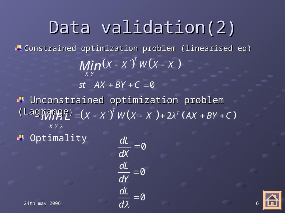
Data validation(2)Data validation(2)Constrained optimization problem (linearised eq)Constrained optimization problem (linearised eq)

' '

,

0

T

X Y

X X W X X

st AX BY C

Min

' '

, ,

2T T

X Y

X X W X X AX BY CMinL

Unconstrained optimization problem (LagrangeUnconstrained optimization problem (Lagrange))

0

0

0

dL

dXdL

dYdL

d

Optimality

7724th may 200624th may 2006

Data validation(3)Data validation(3)

Solve the system:Solve the system:'0

0 0 0

0

T

T

W A X X WX

B Y M Y

A B C

1 ' 1,, ,

1 1

1 ' 1,, ,

1 1

pm

i j j j ki j i n m kj k

pm

i j j j kn i j n i n m kj k

X M W X M C

Y M W X M C

Solution:Solution:

8824th may 200624th may 2006

Data validation(4)Data validation(4)

Validated accuraciesValidated accuracies

21

,

'1

21

,

'1

mi j

ij j

mn i j

ij j

MVar X

Var X

MVar Y

Var X

9924th may 200624th may 2006

Algorithm descriptionAlgorithm description

1var,

1i

j

Ni j

Yj y

MVar

Var

Sensor databaseBelsim-Vali validation model

Optimization criteria

Key variables

Sensor network optimization

Problem feasability?

Sensor requirements

Sensor database

- Cost

- Accepted range

- UncertaintyKey variables

- Variables

- Required standart deviation

Sensor requirements

- existing sensor

- impossible placement

Optimization criteria

- Cost

- Target accuracies

- Singularity of the validation problem

- Safeguard against one sensor failure

- Several operating points

Sensor network optimization

Problem feasability?

For all possible sensors :

-M singular?

-Target accuracies reached?

Belsim-Vali validation model

-For all operating points

-Validated values of all variables

-Jacobian matrices A and B

101024th may 200624th may 2006

OptimizationOptimizationThe problem to optimise isThe problem to optimise is

Large scale

Generally multimodal

Not derivable

Genetic algorithmGenetic algorithm Developed by John Holland

Solution described by a set of binary decisions (genes) corresponding to the decision to install a sensor at a given location

111124th may 200624th may 2006

Optimization(2)Optimization(2)

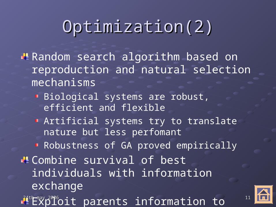
Random search algorithm based on reproduction and natural selection mechanisms

Biological systems are robust, efficient and flexible

Artificial systems try to translate nature but less perfomant

Robustness of GA proved empirically

Combine survival of best individuals with information exchange

Exploit parents information to create better children

121224th may 200624th may 2006

Optimization(3)Optimization(3)

Mecanisms used: Selection

Reproduction (50%)

One-point-crossover (50%)

Jump mutation (1%)

01011 10110

11010 01100 11010 10110

01011 01100

Before single point crossover

After single point crossover

Father

Mother

First child

Second child

01011 1011001011 10110

11010 0110011010 01100 11010 10110

01011 01100

11010 1011011010 10110

01011 0110001011 01100

Before single point crossover

After single point crossover

Father

Mother

First child

Second child0101110110 0101100110

Before jump mutation

After jump mutation

01011101100101110110 01011001100101100110

Before jump mutation

After jump mutation

131324th may 200624th may 2006

Optimization(2)Optimization(2)

First population chosen randomly with a high First population chosen randomly with a high probability for each sensor to be chosenprobability for each sensor to be chosenPopulation of 20 chromosomesPopulation of 20 chromosomesEvaluation of each chromosome’s fitnessEvaluation of each chromosome’s fitness

Sensitivity matrix inversion Sensitivity matrix inversion (Chen et (Chen et Stadherr) Stadherr) sparse matrixsparse matrix

The best individual is kept at each generationThe best individual is kept at each generationStop criterion: best remains unchanged during x Stop criterion: best remains unchanged during x generationsgenerationsFinal solution better than initial one Final solution better than initial one (but not (but not necessary the global minimum)necessary the global minimum)

141424th may 200624th may 2006

Ammonia synthesis loop 224 variables 178 constraint equations 117 potential sensors 58 key parameters

Case study: ammonia loopCase study: ammonia loop

Optimes.exe

151524th may 200624th may 2006

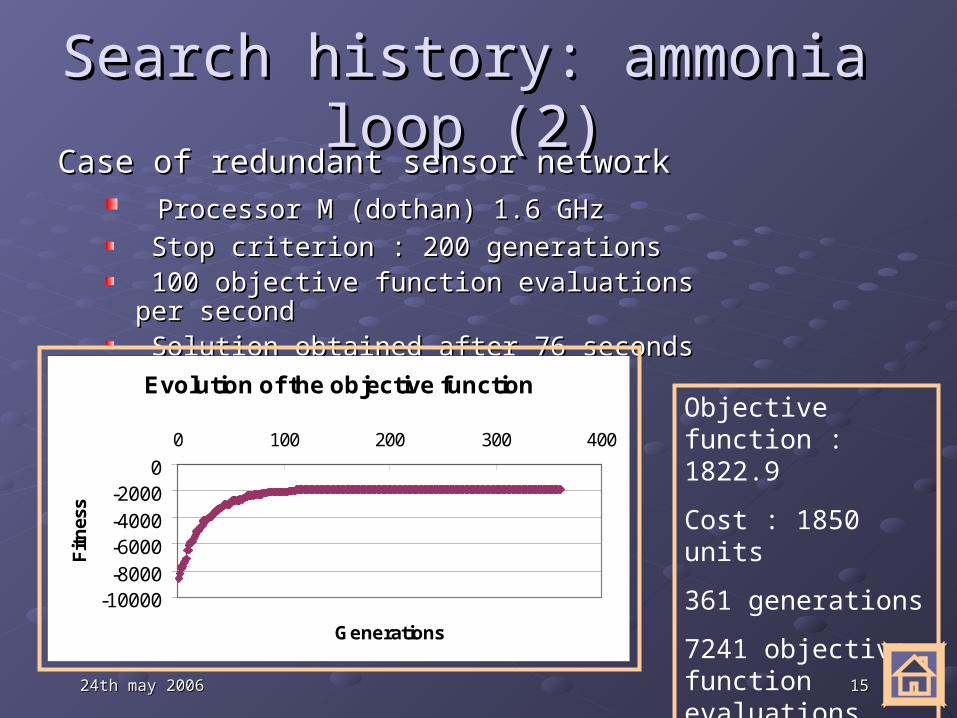
Search history: ammonia loop (2)Search history: ammonia loop (2)Case of redundant sensor networkCase of redundant sensor network

Processor M (dothan) 1.6 GHz Processor M (dothan) 1.6 GHz

Stop criterion : 200 generationsStop criterion : 200 generations 100 objective function evaluations per second100 objective function evaluations per second Solution obtained after 76 secondsSolution obtained after 76 seconds

Objective function : 1822.9

Cost : 1850 units

361 generations

7241 objective function evaluations

Evolution of the objective function

-10000-8000-6000-4000-2000

0

0 100 200 300 400

Generations

Fit

nes

s

161624th may 200624th may 2006

Solution : Solution : case of redundant sensor case of redundant sensor networknetwork

39 sensors :

1 chromatograph,

7 mass flowmeters,

20 temperature sensors,

11 pressure gauges

171724th may 200624th may 2006

Solution : Solution : case of one sensor failurecase of one sensor failure

67 sensors :

2 chromatograph,

13 mass flowmeters,

31 temperature sensors,

21 pressure gauges

Computing time : 1h45

181824th may 200624th may 2006

Case study: reformerCase study: reformer

1263 variables1116 constraint equations473 potential sensors9 key parametersCase of redundant sensor networkCase of redundant sensor network

Processor Pentium IVProcessor Pentium IV Stop criterion : 200 generationsStop criterion : 200 generations 9 objective function evaluations per minut9 objective function evaluations per minut Solution obtained after 6 daysSolution obtained after 6 days

191924th may 200624th may 2006

Case study: reformer (2)Case study: reformer (2)

Objective function : 1955.1 unitsCost : 1960 units1618 generations77665 objective function evaluationsSolution: 72 sensors :

3 chromatographs, 10 mass flowmeters, 45 temperature sensors, 13 pressure gauges,1 density sensor

202024th may 200624th may 2006

ParallelisationParallelisationWhy?Why?

p

Speed upEfficiency

N 1

p

TSpeed up

T

Large computing time for middle size problemsLarge computing time for middle size problems

share the computing work between several share the computing work between several processorsprocessors

reduce the computing timereduce the computing time

techniques are compared by efficiencytechniques are compared by efficiency

ParallelisationParallelisation allows toallows to

Impossible to deal with larger size problemsImpossible to deal with larger size problems

212124th may 200624th may 2006

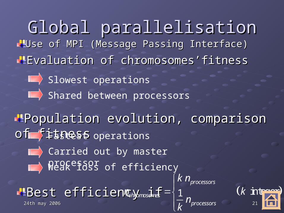
Global parallelisationGlobal parallelisation

Evaluation of chromosomes’fitnessEvaluation of chromosomes’fitness

Population evolution, comparison of Population evolution, comparison of fitnessfitness

Best efficiency if Best efficiency if integer1processors

chromosomes

processors

k nn k

nk

Fastest operations

Use of MPI (Message Passing Interface)Use of MPI (Message Passing Interface)

Carried out by master processor

Weak loss of efficiency

Shared between processors

Slowest operations

222224th may 200624th may 2006

0

50

100

150

200

250

300

350

400

450

0 0.2 0.4 0.61/processors number

Tim

e (s

ec)

40

50

60

70

80

90

100

Eff

icie

ncy

(%

)

Master time

Elapsed time

Efficiency

Global parallelisation Global parallelisation (2)(2)

chromosomes processorsn k nCase of a redundant sensor network:

232324th may 200624th may 2006

Distributed Genetic AlgorithmDistributed Genetic AlgorithmGlobal parallelisation : fall of efficiency with the number of Global parallelisation : fall of efficiency with the number of

processorsprocessors

DGA : better efficiency?DGA : better efficiency?Chromosomes distributed in sub-populationsChromosomes distributed in sub-populations

Migration operator : chromosomes transfertMigration operator : chromosomes transfert

Migrating chromosomes chosen randomlyMigrating chromosomes chosen randomly

Parameters : Parameters : Sub-populations’size: 10 chromosomesSub-populations’size: 10 chromosomes

Number of migrating chromosomes : 2Number of migrating chromosomes : 2

Number of sub-populations : 5Number of sub-populations : 5

Number of generations before migration : 5Number of generations before migration : 5

Influence of the number of iterations between two migrations

0

500

1000

1500

2000

0 5 10 15 20 25

Number of iterations between two migrations

Total number of iterations

Master time(sec)

Objectif function

Influence of the number of 10 chromosoms sub-populations

0300600900

120015001800

0 5 10

Number of sub-populations

Total number of iterations

Master time (sec)

Objectif function

242424th may 200624th may 2006

Results comparisonResults comparisonTime comparison between global

parallelisation and distributed algorithm

0100

200300

400500

600700

800

0 2 4 6 8 10

Number of processors or sub-populations

Tim

e (s

ec)

Global parallelisation : master time

Global parallelisation : elapsed timeDistributed algorithm : master time

Distributed algorithm : elapsed time

Efficiency comparison

0.7

0.8

0.9

1

1.1

1.2

1.3

0 2 4 6 8 10

Number of sub-populations or processors

Eff

icie

ncy

Global parallelisation: efficiency

Distributed algorithm: efficiency

252524th may 200624th may 2006

ConclusionsConclusions

The solution found is better than the initial The solution found is better than the initial network but there is no guarantee of network but there is no guarantee of overall optimumoverall optimumAccuracies on key parameters are Accuracies on key parameters are acceptableacceptableBoth parallelization techniques allow to Both parallelization techniques allow to reduce the computing timereduce the computing timeDistributed genetic algorithm gives better Distributed genetic algorithm gives better results than global parallelizationresults than global parallelization

262624th may 200624th may 2006

Future workFuture work

Adaptation to dynamic problemsAdaptation to dynamic problems

Create an algorithm of dynamic data Create an algorithm of dynamic data validationvalidation

Design of networks able to identify Design of networks able to identify process faultsprocess faults

272724th may 200624th may 2006

AcknowledgementsAcknowledgements

Walloon RegionWalloon Region

European Social FundsEuropean Social Funds

282824th may 200624th may 2006

Questions?Questions?