22 Linear Programming

1

Linear Programming

brewer’s problemsimplex algorithmimplementationlinear programming

References:

The Allocation of Resources by Linear Programming,

Scientific American, by Bob Bland

Algs in Java, Part 5

Overview: introduction to advanced topics

Main topics

• linear programming: the ultimate practical problem-solving model

• reduction: design algorithms, prove limits, classify problems

• NP: the ultimate theoretical problem-solving model

• combinatorial search: coping with intractability

Shifting gears

• from linear/quadratic to polynomial/exponential scale

• from individual problems to problem-solving models

• from details of implementation to conceptual framework

Goals

• place algorithms we’ve studied in a larger context

• introduce you to important and essential ideas

• inspire you to learn more about algorithms!

2

3

Linear Programming

What is it?

• Quintessential tool for optimal allocation of scarce resources, among

a number of competing activities.

• Powerful and general problem-solving method that encompasses:

shortest path, network flow, MST, matching, assignment...

Ax = b, 2-person zero sum games

Why significant?

• Widely applicable problem-solving model

• Dominates world of industry.

• Fast commercial solvers available: CPLEX, OSL.

• Powerful modeling languages available: AMPL, GAMS.

• Ranked among most important scientific advances of 20th century.

see ORF 307

Ex: Delta claims that LPsaves $100 million per year.

4

Applications

Agriculture. Diet problem.

Computer science. Compiler register allocation, data mining.

Electrical engineering. VLSI design, optimal clocking.

Energy. Blending petroleum products.

Economics. Equilibrium theory, two-person zero-sum games.

Environment. Water quality management.

Finance. Portfolio optimization.

Logistics. Supply-chain management.

Management. Hotel yield management.

Marketing. Direct mail advertising.

Manufacturing. Production line balancing, cutting stock.

Medicine. Radioactive seed placement in cancer treatment.

Operations research. Airline crew assignment, vehicle routing.

Physics. Ground states of 3-D Ising spin glasses.

Plasma physics. Optimal stellarator design.

Telecommunication. Network design, Internet routing.

Sports. Scheduling ACC basketball, handicapping horse races.

5


6

Toy LP example: Brewer’s problem

Small brewery produces ale and beer.

• Production limited by scarce resources: corn, hops, barley malt.

• Recipes for ale and beer require different proportions of resources.

Brewer’s problem: choose product mix to maximize profits.

corn (lbs) hops (oz) malt (lbs) profit ($)

available 480 160 1190

ale (1 barrel) 5 4 35 13

beer (1 barrel) 15 4 20 23

all ale (34 barrels)

179 136 1190 442

all beer(32 barrels)

480 128 640 736

20 barrels ale20 barrels beer

400 160 1100 720

12 barrels ale28 barrels beer

480 160 980 800

more profitableproduct mix?

? ? ? >800 ?

34 barrels times 35 lbs maltper barrel is 1190 lbs

[ amount of available malt ]

7

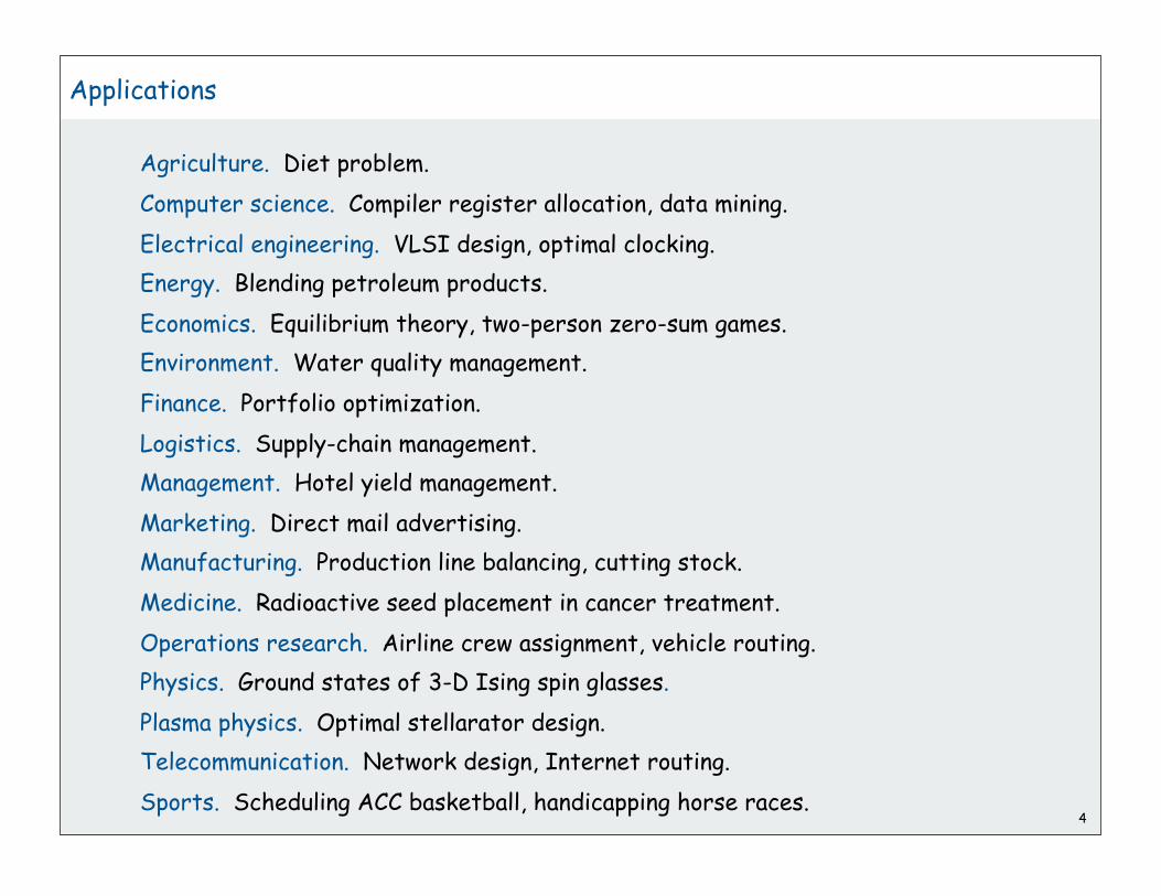
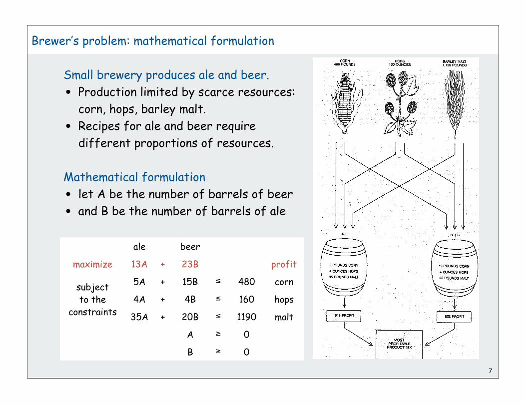
Brewer’s problem: mathematical formulation

ale beer

maximize 13A + 23B profit

subjectto the

constraints

5A + 15B 480 corn

4A + 4B 160 hops

35A + 20B 1190 malt

A 0

B 0

Small brewery produces ale and beer.

• Production limited by scarce resources:

corn, hops, barley malt.

• Recipes for ale and beer require

different proportions of resources.

Mathematical formulation

• let A be the number of barrels of beer

• and B be the number of barrels of ale

8

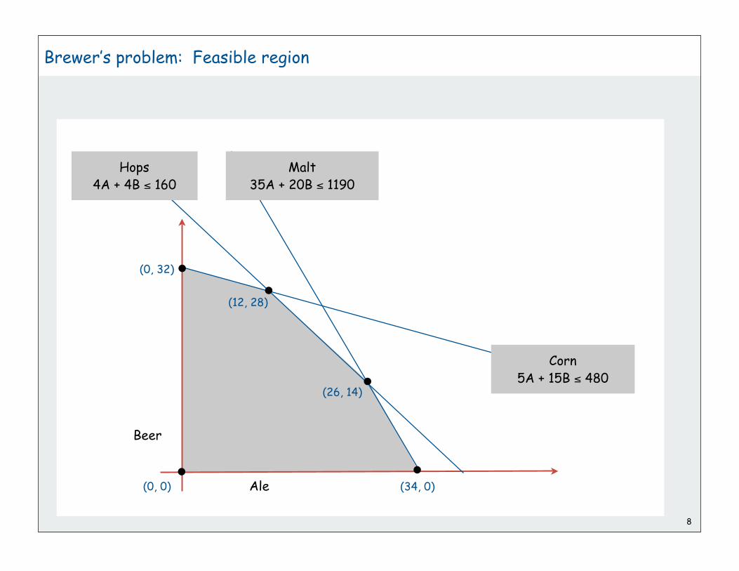
Brewer’s problem: Feasible region

Ale

Beer

(34, 0)

(0, 32)

Corn5A + 15B 480

Hops4A + 4B 160

Malt35A + 20B 1190

(12, 28)

(26, 14)

(0, 0)

9

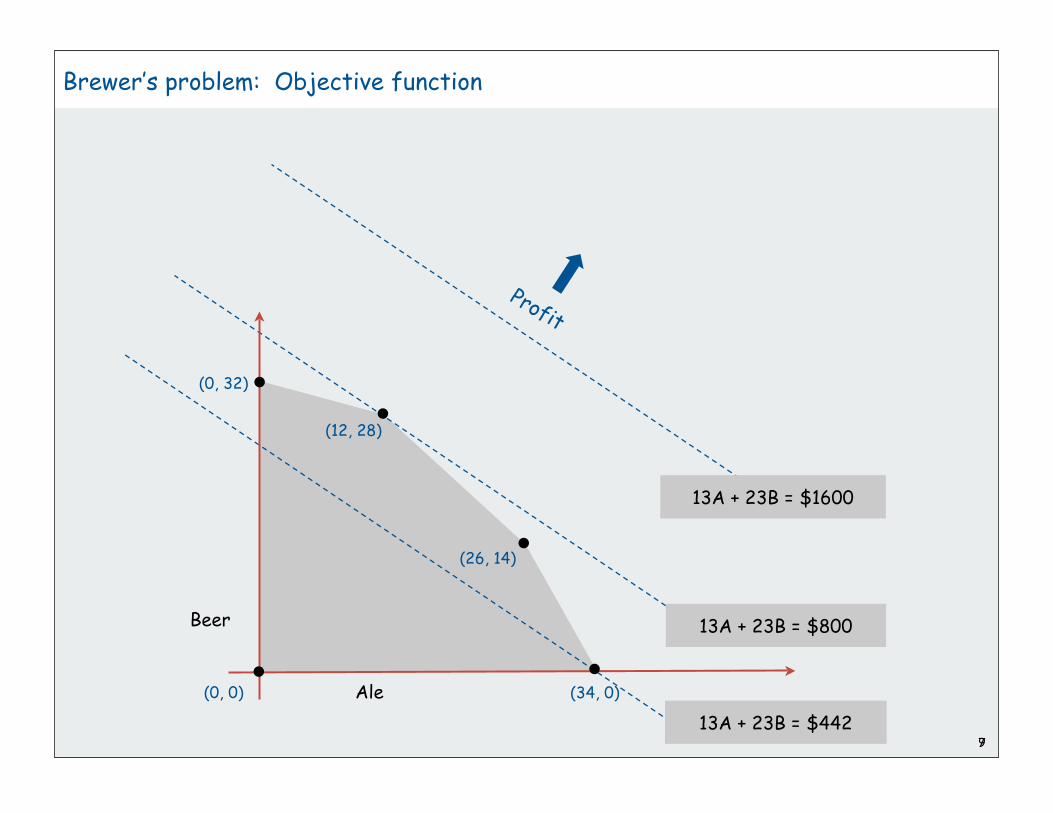
Brewer’s problem: Objective function

13A + 23B = $800

13A + 23B = $1600

13A + 23B = $442

Profit

Ale

Beer

7

(34, 0)

(0, 32)

(12, 28)

(26, 14)

(0, 0)

10

Brewer’s problem: Geometry

Brewer’s problem observation. Regardless of objective function

coefficients, an optimal solution occurs at an extreme point.

extreme point

Ale

Beer

7

(34, 0)

(0, 32)

(12, 28)

(26, 14)

(0, 0)

11

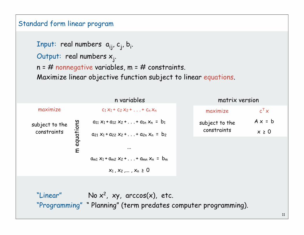
Standard form linear program

Input: real numbers aij, cj, bi.

Output: real numbers xj.

n = # nonnegative variables, m = # constraints.

Maximize linear objective function subject to linear equations.

“Linear” No x2, xy, arccos(x), etc.

“Programming” “ Planning” (term predates computer programming).

maximize c1 x1 + c2 x2 + . . . + cn xn

subject to the constraints

a11 x1 + a12 x2 + . . . + a1n xn = b1

a21 x1 + a22 x2 + . . . + a2n xn = b2

...

am1 x1 + am2 x2 + . . . + amn xn = bm

x1 , x2 ,... , xn 0

n variables

m e

quat

ions

maximize cT x

subject to the constraints

A x = b

x 0

matrix version

12

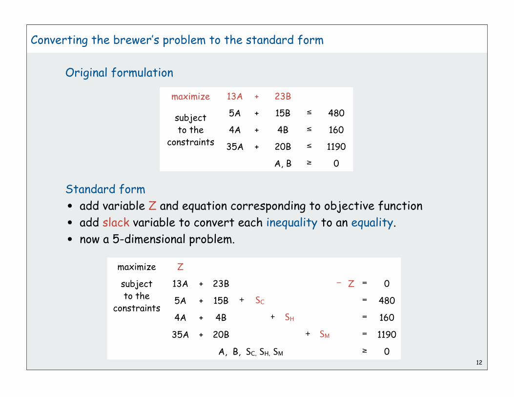
Converting the brewer’s problem to the standard form

Original formulation

Standard form

• add variable Z and equation corresponding to objective function

• add slack variable to convert each inequality to an equality.

• now a 5-dimensional problem.

maximize 13A + 23B

subjectto the

constraints

5A + 15B 480

4A + 4B 160

35A + 20B 1190

A, B 0

maximize Z

subjectto the

constraints

13A + 23B Z = 0

5A + 15B + SC = 480

4A + 4B + SH = 160

35A + 20B + SM = 1190

A, B, SC, SH, SM 0

13

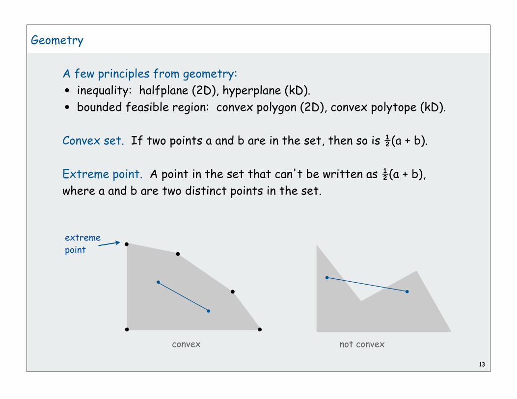
A few principles from geometry:

• inequality: halfplane (2D), hyperplane (kD).

• bounded feasible region: convex polygon (2D), convex polytope (kD).

Convex set. If two points a and b are in the set, then so is (a + b).

Extreme point. A point in the set that can't be written as (a + b),

where a and b are two distinct points in the set.

Geometry

convex not convex

extremepoint

14

Geometry (continued)

Extreme point property. If there exists an optimal solution to (P),

then there exists one that is an extreme point.

Good news. Only need to consider finitely many possible solutions.

Bad news. Number of extreme points can be exponential !

Greedy property. Extreme point is optimal

iff no neighboring extreme point is better.

local optima are global optima

Ex: n-dimensional hypercube

15


16

Simplex Algorithm

Simplex algorithm. [George Dantzig, 1947]

• Developed shortly after WWII in response to logistical problems,

including Berlin airlift.

• One of greatest and most successful algorithms of all time.

Generic algorithm.

• Start at some extreme point.

• Pivot from one extreme point to a neighboring one.

• Repeat until optimal.

How to implement? Linear algebra.

never decreasing objective function

17

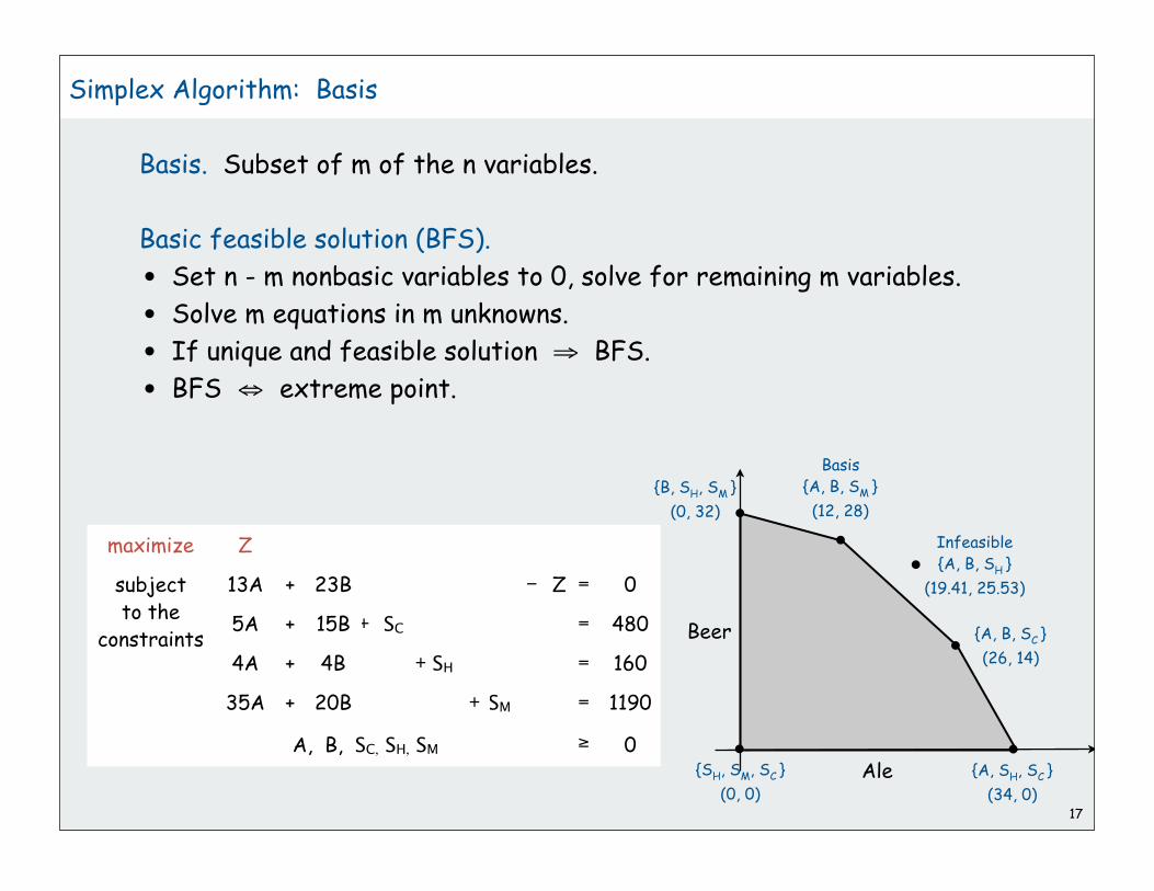
Simplex Algorithm: Basis

Basis. Subset of m of the n variables.

Basic feasible solution (BFS).

• Set n - m nonbasic variables to 0, solve for remaining m variables.

• Solve m equations in m unknowns.

• If unique and feasible solution BFS.

• BFS extreme point.

Ale

Beer

Basis{A, B, SM }

(12, 28)

{A, B, SC }

(26, 14)

{B, SH, SM }

(0, 32)

{SH, SM, SC }

(0, 0)

{A, SH, SC }

(34, 0)

Infeasible{A, B, SH }

(19.41, 25.53)

maximize Z

subjectto the

constraints

13A + 23B Z = 0

5A + 15B + SC = 480

4A + 4B + SH = 160

35A + 20B + SM = 1190

A, B, SC, SH, SM 0

18

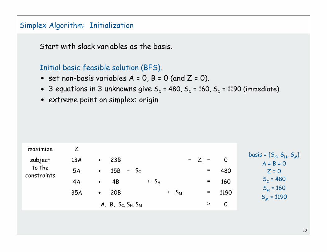
Simplex Algorithm: Initialization

basis = {SC, SH, SM}

A = B = 0Z = 0

SC = 480

SH = 160

SM = 1190

maximize Z

subjectto the

constraints

13A + 23B Z = 0

5A + 15B + SC = 480

4A + 4B + SH = 160

35A + 20B + SM = 1190

A, B, SC, SH, SM 0

Start with slack variables as the basis.

Initial basic feasible solution (BFS).

• set non-basis variables A = 0, B = 0 (and Z = 0).

• 3 equations in 3 unknowns give SC = 480, SC = 160, SC = 1190 (immediate).

• extreme point on simplex: origin


A = B = 0Z = 0

SC = 480

SH = 160

SM = 1190

maximize Z

subjectto the

constraints

13A + 23B Z = 0

5A + 15B + SC = 480

4A + 4B + SH = 160

35A + 20B + SM = 1190

A, B, SC, SH, SM 0

19

Simplex Algorithm: Pivot 1

Substitution B = (1/15)(480 – 5A – SC ) puts B into the basis

( rewrite 2nd equation, eliminate B in 1st, 3rd, and 4th equations)

basis = {B, SH, SM}

A = SC = 0

Z = 736B = 32 SH = 32

SM = 550

maximize Z

subjectto the

constraints

(16/3)A - (23/15) SC Z = -736

(1/3) A + B + (1/15) SC = 32

(8/3) A - (4/15) SC + SH = 32

(85/3) A - (4/3) SC+ SM = 550

A, B, SC, SH, SM 0

which variable does it replace?

20


Why pivot on B?

• Its objective function coefficient is positive

(each unit increase in B from 0 increases objective value by $23)

• Pivoting on column 1 also OK.

Why pivot on row 2?

• Preserves feasibility by ensuring RHS 0.

• Minimum ratio rule: min { 480/15, 160/4, 1190/20 }.


A = B = 0Z = 0

SC = 480

SH = 160

SM = 1190

maximize Z

subjectto the

constraints

13A + 23B Z = 0

5A + 15B + SC = 480

4A + 4B + SH = 160

35A + 20B + SM = 1190

A, B, SC, SH, SM 0

basis = {B, SH, SM}

A = SC = 0

Z = 736B = 32 SH = 32

SM = 550

maximize Z

subjectto the

constraints

(16/3)A - (23/15) SC Z = -736

(1/3) A + B + (1/15) SC = 32

(8/3) A - (4/15) SC + SH = 32

(85/3) A - (4/3) SC + SM = 550

A, B, SC, SH, SM 0

21


basis = {A, B, SM}

SC = SH = 0

Z = 800B = 28 A = 12

SM = 110

maximize Z

subjectto the

constraints

- SC - 2SH Z = -800

B + (1/10) SC + (1/8) SH = 28

A - (1/10) SC + (3/8) SH = 12

- (25/6) SC - (85/8) SH + SM = 110

A, B, SC, SH, SM 0

Substitution A = (3/8)(32 + (4/15) SC – SH ) puts A into the basis

( rewrite 3nd equation, eliminate A in 1st, 2rd, and 4th equations)

22

Simplex algorithm: Optimality

Q. When to stop pivoting?

A. When all coefficients in top row are non-positive.

Q. Why is resulting solution optimal?

A. Any feasible solution satisfies system of equations in tableaux.

• In particular: Z = 800 – SC – 2 SH

• Thus, optimal objective value Z* 800 since SC, SH 0.

• Current BFS has value 800 optimal.

basis = {A, B, SM}

SC = SH = 0

Z = 800B = 28 A = 12

SM = 110

maximize Z

subjectto the

constraints

- SC - 2SH Z = -800

B + (1/10) SC + (1/8) SH = 28

A - (1/10) SC + (3/8) SH = 12

- (25/6) SC - (85/8) SH + SM = 110

A, B, SC, SH, SM 0

23


Encode standard form LP in a single Java 2D array

Simplex tableau

24

A

c

bI

0 0

m

1

n m 1

maximize Z

subjectto the

constraints

13A + 23B Z = 0

5A + 15B + SC = 480

4A + 4B + SH = 160

35A + 20B + SM = 1190

A, B, SC, SH, SM 0

5 15 1 0 0 480

4 4 0 1 0 160

35 20 0 0 1 1190

13 23 0 0 0 0

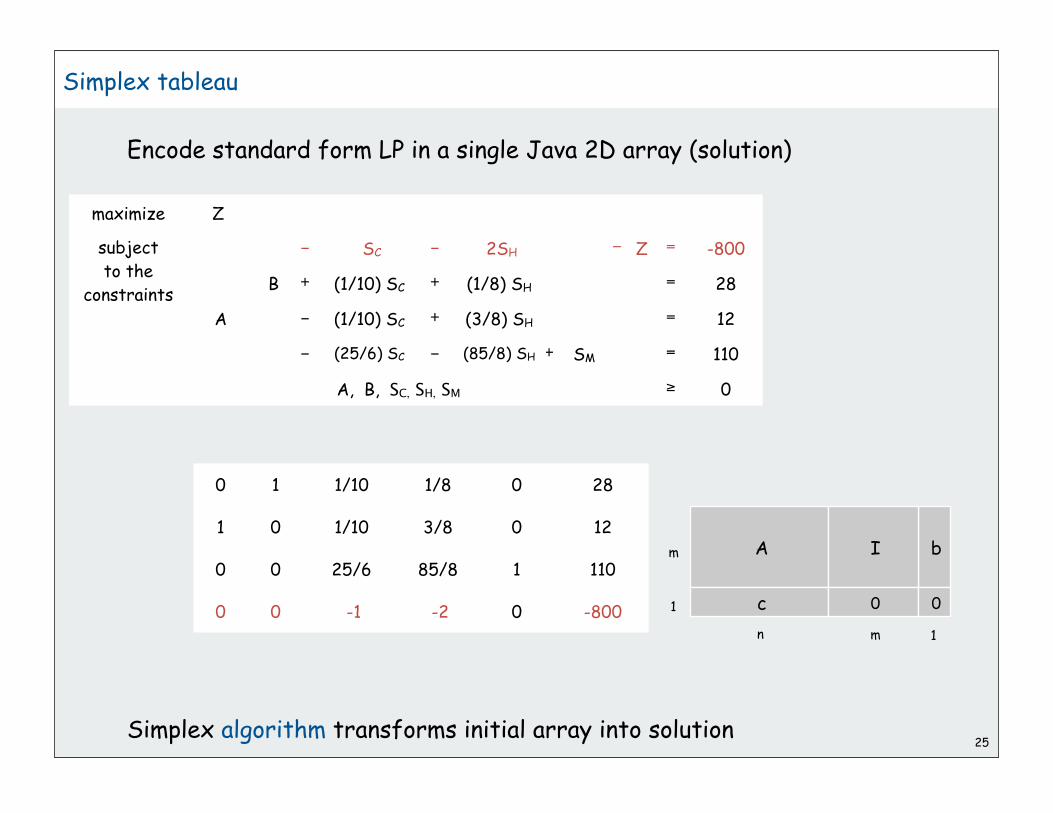
Encode standard form LP in a single Java 2D array (solution)

Simplex algorithm transforms initial array into solution

Simplex tableau

25

A

c

bI

0 0

m

1

n m 1

0 1 1/10 1/8 0 28

1 0 1/10 3/8 0 12

0 0 25/6 85/8 1 110

0 0 -1 -2 0 -800

maximize Z

subjectto the

constraints

- SC - 2SH Z = -800

B + (1/10) SC + (1/8) SH = 28

A - (1/10) SC + (3/8) SH = 12

- (25/6) SC - (85/8) SH + SM = 110

A, B, SC, SH, SM 0

26

Simplex algorithm: Bare-bones implementation

Construct the simplex tableau.

A

c

bI

0 0

public class Simplex{ private double[][] a; // simplex tableaux private int M, N;

public Simplex(double[][] A, double[] b, double[] c) { M = b.length; N = c.length; a = new double[M+1][M+N+1]; for (int i = 0; i < M; i++) for (int j = 0; j < N; j++) a[i][j] = A[i][j]; for (int j = N; j < M + N; j++) a[j-N][j] = 1.0; for (int j = 0; j < N; j++) a[M][j] = c[j]; for (int i = 0; i < M; i++) a[i][M+N] = b[i]; }

m

1

n m 1

put A[][] into tableau

put I[] into tableauput c[] into tableauput b[] into tableau

constructor

27

Simplex algorithm: Bare-bones Implementation

Pivot on element (p, q).

public void pivot(int p, int q){ for (int i = 0; i <= M; i++) for (int j = 0; j <= M + N; j++) if (i != p && j != q) a[i][j] -= a[p][j] * a[i][q] / a[p][q]; for (int i = 0; i <= M; i++) if (i != p) a[i][q] = 0.0;

for (int j = 0; j <= M + N; j++) if (j != q) a[p][j] /= a[p][q]; a[p][q] = 1.0;}

p

q

scale all elements butrow p and column q

zero out column q

scale row p

28

Simplex Algorithm: Bare Bones Implementation

Simplex algorithm.

find entering variable q(positive objective function coefficient)

find row p accordingto min ratio rule

+p

q

+

+

public void solve(){ while (true) { int p, q; for (q = 0; q < M + N; q++) if (a[M][q] > 0) break; if (q >= M + N) break;

for (p = 0; p < M; p++) if (a[p][q] > 0) break; for (int i = p+1; i < M; i++) if (a[i][q] > 0) if (a[i][M+N] / a[i][q] < a[p][M+N] / a[p][q]) p = i; pivot(p, q); }}

min ratio test

29

Simplex Algorithm: Running Time

Remarkable property. In practice, simplex algorithm typically

terminates after at most 2(m+n) pivots.

• No pivot rule that is guaranteed to be polynomial is known.

• Most pivot rules known to be exponential (or worse) in worst-case.

Pivoting rules. Carefully balance the cost of finding an entering

variable with the number of pivots needed.

30

Simplex algorithm: Degeneracy

Degeneracy. New basis, same extreme point.

Cycling. Get stuck by cycling through different bases that all

correspond to same extreme point.

• Doesn't occur in the wild.

• Bland's least index rule guarantees finite # of pivots.

"stalling" is common in practice

To improve the bare-bones implementation

• Avoid stalling.

• Choose the pivot wisely.

• Watch for numerical stability.

• Maintain sparsity.

• Detect infeasiblity

• Detect unboundedness.

• Preprocess to reduce problem size.

Basic implementations available in many programming environments.

Commercial solvers routinely solve LPs with millions of variables.

requires fancy data structures

31

Simplex Algorithm: Implementation Issues

Ex. 1: OR-Objects Java library

Ex. 2: MS Excel (!)32

import drasys.or.mp.*; import drasys.or.mp.lp.*;

public class LPDemo{ public static void main(String[] args) throws Exception { Problem prob = new Problem(3, 2); prob.getMetadata().put("lp.isMaximize", "true"); prob.newVariable("x1").setObjectiveCoefficient(13.0); prob.newVariable("x2").setObjectiveCoefficient(23.0); prob.newConstraint("corn").setRightHandSide( 480.0); prob.newConstraint("hops").setRightHandSide( 160.0); prob.newConstraint("malt").setRightHandSide(1190.0); prob.setCoefficientAt("corn", "x1", 5.0); prob.setCoefficientAt("corn", "x2", 15.0); prob.setCoefficientAt("hops", "x1", 4.0); prob.setCoefficientAt("hops", "x2", 4.0); prob.setCoefficientAt("malt", "x1", 35.0); prob.setCoefficientAt("malt", "x2", 20.0); DenseSimplex lp = new DenseSimplex(prob); System.out.println(lp.solve()); System.out.println(lp.getSolution()); }}

LP solvers: basic implementations

33

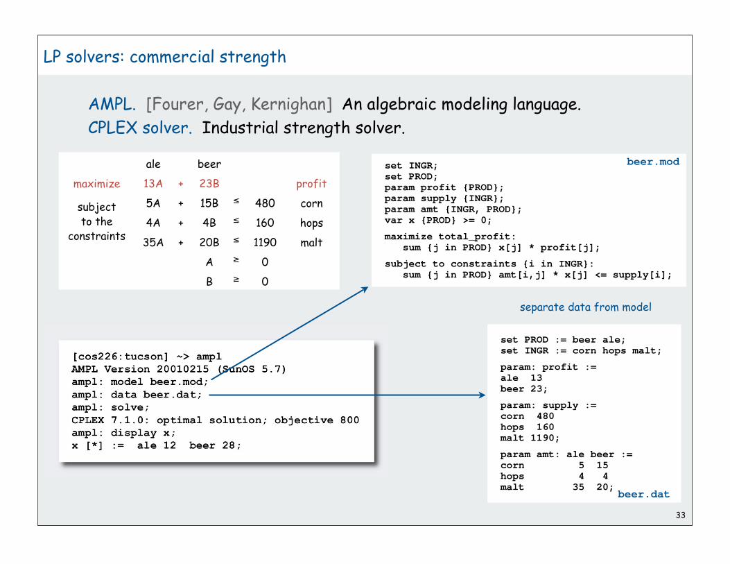
set PROD := beer ale;set INGR := corn hops malt;

param: profit :=ale 13beer 23;

param: supply :=corn 480hops 160malt 1190;

param amt: ale beer :=corn 5 15hops 4 4malt 35 20;

LP solvers: commercial strength

AMPL. [Fourer, Gay, Kernighan] An algebraic modeling language.

CPLEX solver. Industrial strength solver.

set INGR;set PROD;param profit {PROD};param supply {INGR};param amt {INGR, PROD};var x {PROD} >= 0;

maximize total_profit: sum {j in PROD} x[j] * profit[j];

subject to constraints {i in INGR}: sum {j in PROD} amt[i,j] * x[j] <= supply[i];

beer.dat

beer.mod

separate data from model

ale beer

maximize 13A + 23B profit

subjectto the

constraints

5A + 15B 480 corn

4A + 4B 160 hops

35A + 20B 1190 malt

A 0

B 0

34

History

1939. Production, planning. [Kantorovich]

1947. Simplex algorithm. [Dantzig]

1950. Applications in many fields.

1979. Ellipsoid algorithm. [Khachian]

1984. Projective scaling algorithm. [Karmarkar]

1990. Interior point methods.

• Interior point faster when polyhedron smooth like disco ball.

• Simplex faster when polyhedron spiky like quartz crystal.

200x. Approximation algorithms, large scale optimization.

35


Linear programming

Linear “programming”

• process of formulating an LP model for a problem

• solution to LP for a specific problem gives solution to the problem

1. Identify variables

2. Define constraints (inequalities and equations)

3. Define objective function

Examples:

• shortest paths

• maxflow

• bipartite matching

• .

• .

• .

• [ a very long list ]

36

easy part [omitted]:convert to standard form

stay tuned [this lecture]

37

Single-source shortest-paths problem (revisited)

Given. Weighted digraph, single source s.

Distance from s to v: length of the shortest path from s to v .

Goal. Find distance (and shortest path) from s to every other vertex.

s

3

t

2

6

7

4

5

24

18

2

9

14

155

30

20

44

16

11

6

19

6

LP formulation of single-source shortest-paths problem

38

s

3

t

2

6

7

4

5

24

18

2

9

14

155

30

20

44

16

11

6

19

6

minimize xt

subjectto the

constraints

xs + 9 x2

xs + 14 x6

xs + 15 x7

x2 + 24 x3

x3 + 2 x5

x3 + 19 xt

x4 + 6 x3

x4 + 6 xt

x5 + 11 x4

x5 + 16 xt

x6 + 18 x3

x6 + 30 x5

x6 + 5 x7

x7 + 20 x5

x7 + 44 xt

xs = 0

x2 , ... , xt 0

One variable per vertex, one inequality per edge.

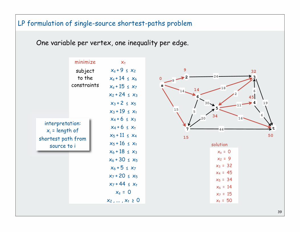
LP formulation of single-source shortest-paths problem

39

s

3

t

2

6

7

4

5

24

18

2

9

14

155

30

20

44

16

11

6

19

6

0

9 32

14

15 50

34

45

minimize xt

subjectto the

constraints

xs + 9 x2

xs + 14 x6

xs + 15 x7

x2 + 24 x3

x3 + 2 x5

x3 + 19 xt

x4 + 6 x3

x4 + 6 xt

x5 + 11 x4

x5 + 16 xt

x6 + 18 x3

x6 + 30 x5

x6 + 5 x7

x7 + 20 x5

x7 + 44 xt

xs = 0

x2 , ... , xt 0

xs = 0

x2 = 9

x3 = 32

x4 = 45

x5 = 34

x6 = 14

x7 = 15

xt = 50

solution

One variable per vertex, one inequality per edge.

3

3

40

Maxflow problem

Given: Weighted digraph, source s, destination t.

Interpret edge weights as capacities

• Models material flowing through network

• Ex: oil flowing through pipes

• Ex: goods in trucks on roads

• [many other examples]

Flow: A different set of edge weights

• flow does not exceed capacity in any edge

• flow at every vertex satisfies equilibrium

[ flow in equals flow out ]

Goal: Find maximum flow from s to t

2 3

1

2

s

1

3 4

2

t

1 1

s

1

3 4

2

t

flow out of s is 3

flow in to t is 3

1 2

10

1 1

2 1

flow capacityin every edge

flow inequals

flow outat each vertex

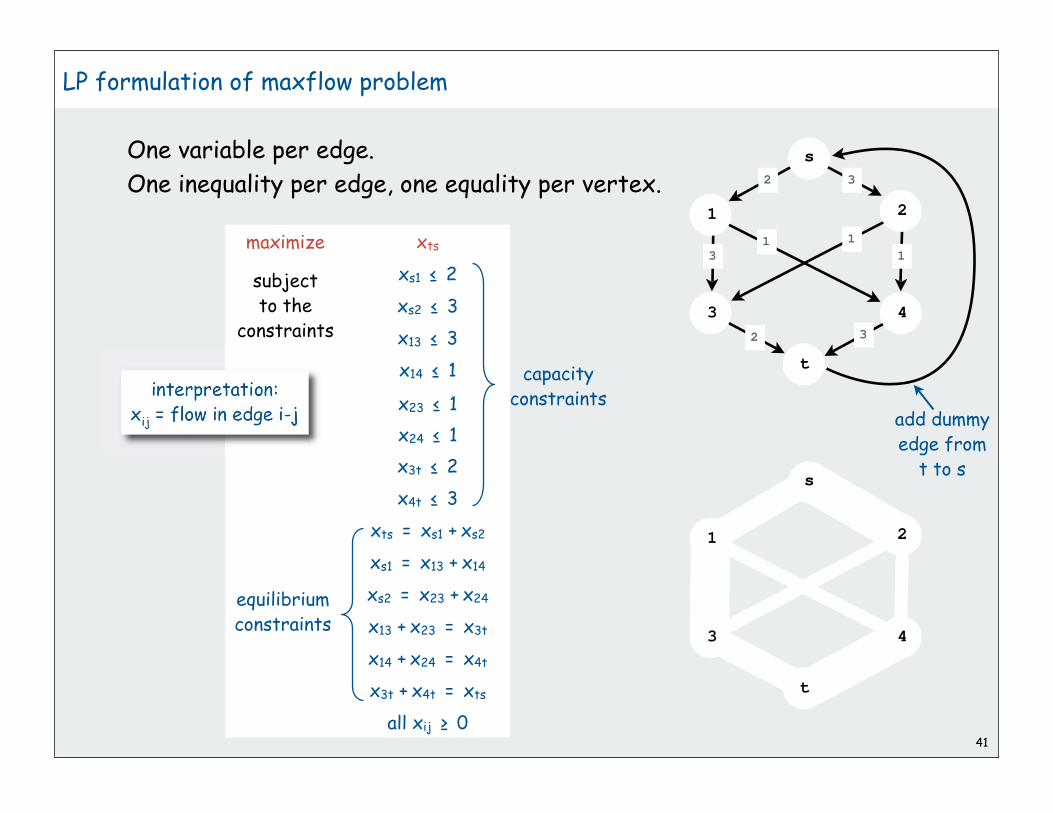
LP formulation of maxflow problem

41

maximize xts

subjectto the

constraints

xs1 2

xs2 3

x13 3

x14 1

x23 1

x24 1

x3t 2

x4t 3

xts = xs1 + xs2

xs1 = x13 + x14

xs2 = x23 + x24

x13 + x23 = x3t

x14 + x24 = x4t

x3t + x4t = xts

all xij 0

One variable per edge.

One inequality per edge, one equality per vertex.

3

3

2 3

1

2

s

1

3 4

2

t

1 1

s

1

3 4

2

t

add dummyedge from

t to s

equilibriumconstraints

capacityconstraints

1

2 2

11

1

2 2

LP formulation of maxflow problem

42

maximize xts

subjectto the

constraints

xs1 2

xs2 3

x13 3

x14 1

x23 1

x24 1

x3t 2

x4t 3

xts = xs1 + xs2

xs1 = x13 + x14

xs2 = x23 + x24

x13 + x23 = x3t

x14 + x24 = x4t

x3t + x4t = xts

all xij 0

xs1 = 2

xs2 = 2

x13 = 1

x14 = 1

x23 = 1

x24 = 1

x3t = 2

x4t = 2

xts = 4

solution

One variable per edge.

One inequality per edge, one equality per vertex.

3

3

2 3

1

2

s

1

3 4

2

t

1 1

s

1

3 4

2

t

add dummyedge from

t to s

maxflow value

equilibriumconstraints

capacityconstraints

Maximum cardinality bipartite matching problem

Given: Two sets of vertices, set of edges

(each connecting one vertex in each set)

Matching: set of edges

with no vertex appearing twice

Interpretation: mutual preference constraints

• Ex: people to jobs

• Ex: medical students to residence positions

• Ex: students to writing seminars

• [many other examples]

Goal: find a maximum cardinality matching

43

A B C D E F

0 1 2 3 4 5

Alice

Adobe, Apple, Google

Bob

Adobe, Apple, Yahoo

Carol

Google, IBM, Sun

Dave

Adobe, Apple

Eliza

IBM, Sun, Yahoo

Frank

Google, Sun, Yahoo

Example: Job offers

Adobe

Alice, Bob, Dave

Apple

Alice, Bob, Dave

Google

Alice, Carol, Frank

IBM

Carol, Eliza

Sun

Carol, Eliza, Frank

Yahoo

Bob, Eliza, Frank

A B C D E F

0 1 2 3 4 5

LP formulation of maximum cardinality bipartite matching problem

44

maximizexA0 + xA1 + xA2 + xB0 + xB1 + xB5

+ xC2 + xC3 + xC4 + xD0 + xD1

+ xE3 + xE4 + xE5 + xF2 + xF4 + xF5

subjectto the

constraints

xA0 + xA1 + xA2 = 1

xB0 + xB1 + xB5 = 1

xC2 + xC3 + xC4 = 1

xD0 + xD1 = 1

xE3 + xE4 + xE5 = 1

xF2 + xF4 + xF5 = 1

xA0 + xB0 + xD0 = 1

xA1 + xB1 + xD1 = 1

xA2 + xC2 + xF2 = 1

xC3 + xE3 = 1

xC4 + xE4 + xF4 = 1

xB5 + xE5 + xF5 = 1

all xij 0

One variable per edge, one equality per vertex.

constraints on top vertices

A B C D E F

0 1 2 3 4 5

Theorem. [Birkhoff 1946, von Neumann 1953]

All extreme points of the above polyhedron have integer (0 or 1) coordinates

Corollary. Can solve bipartite matching problem by solving LP

constraints on bottom vertices

Crucial point: not always so lucky!

LP formulation of maximum cardinality bipartite matching problem

45

maximizexA0 + xA1 + xA2 + xB0 + xB1 + xB5

+ xC2 + xC3 + xC4 + xD0 + xD1

+ xE3 + xE4 + xE5 + xF2 + xF4 + xF5

subjectto the

constraints

xA0 + xA1 + xA2 = 1

xB0 + xB1 + xB5 = 1

xC2 + xC3 + xC4 = 1

xD0 + xD1 = 1

xE3 + xE4 + xE5 = 1

xF2 + xF4 + xF5 = 1

xA0 + xB0 + xD0 = 1

xA1 + xB1 + xD1 = 1

xA2 + xC2 + xF2 = 1

xC3 + xE3 = 1

xC4 + xE4 + xF4 = 1

xB5 + xE5 + xF5 = 1

all xij 0

One variable per edge, one equality per vertex. A B C D E F

0 1 2 3 4 5

A B C D E F

0 1 2 3 4 5

xA1 = 1

xB5 = 1

xC2 = 1

xD0 = 1

xE3 = 1

xF4 = 1

all other xij = 0

solution

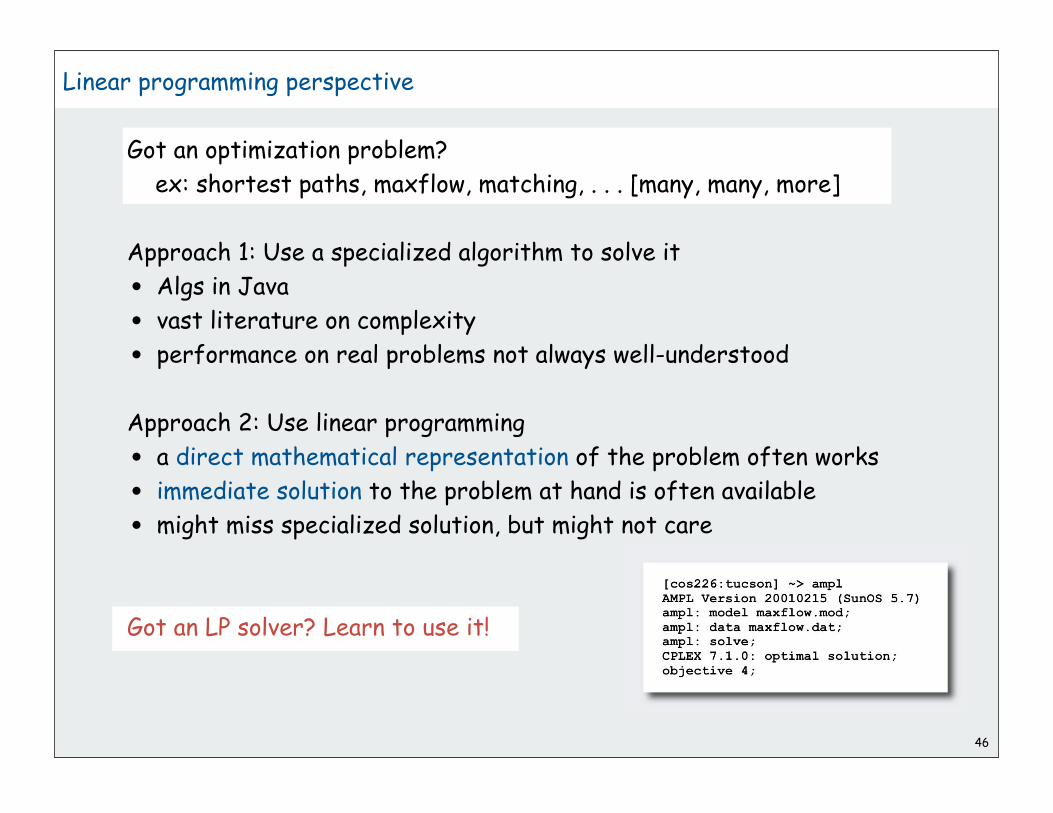
Linear programming perspective

Got an optimization problem?

ex: shortest paths, maxflow, matching, . . . [many, many, more]

Approach 1: Use a specialized algorithm to solve it

• Algs in Java

• vast literature on complexity

• performance on real problems not always well-understood

Approach 2: Use linear programming

• a direct mathematical representation of the problem often works

• immediate solution to the problem at hand is often available

• might miss specialized solution, but might not care

Got an LP solver? Learn to use it!

46

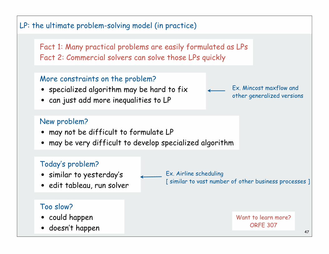
LP: the ultimate problem-solving model (in practice)

Fact 1: Many practical problems are easily formulated as LPs

Fact 2: Commercial solvers can solve those LPs quickly

More constraints on the problem?

• specialized algorithm may be hard to fix

• can just add more inequalities to LP

New problem?

• may not be difficult to formulate LP

• may be very difficult to develop specialized algorithm

Today’s problem?

• similar to yesterday’s

• edit tableau, run solver

Too slow?

• could happen

• doesn’t happen47

Ex. Airline scheduling[ similar to vast number of other business processes ]

Ex. Mincost maxflow and other generalized versions

Want to learn more? ORFE 307

48

Is there an ultimate problem-solving model?

• Shortest paths

• Maximum flow

• Bipartite matching

• . . .

• Linear programming

• .

• .

• .

• NP-complete problems

• .

• .

• .

Does P = NP? No universal problem-solving model exists unless P = NP.

tractable

Ultimate problem-solving model (in theory)

[see next lecture]

intractable ?

Want to learn more? COS 423

49

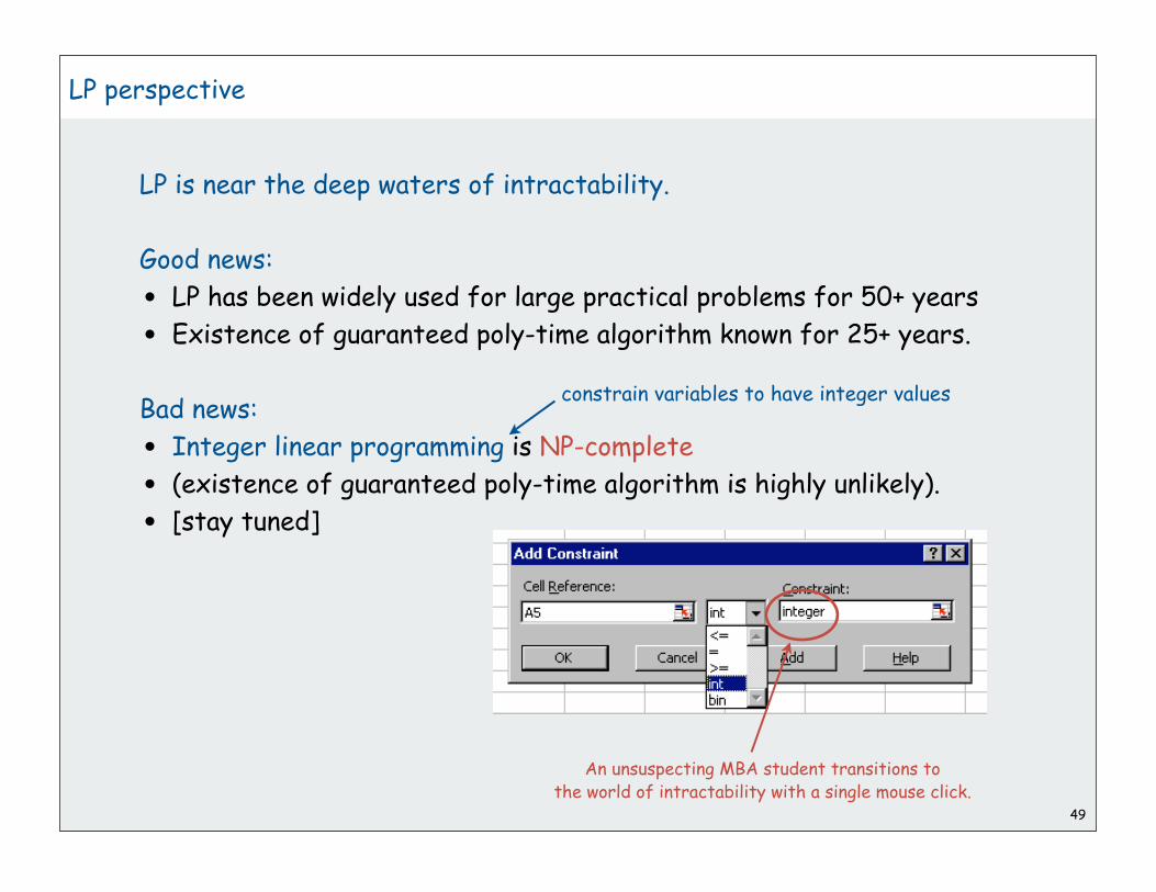
LP perspective

LP is near the deep waters of intractability.

Good news:

• LP has been widely used for large practical problems for 50+ years

• Existence of guaranteed poly-time algorithm known for 25+ years.

Bad news:

• Integer linear programming is NP-complete

• (existence of guaranteed poly-time algorithm is highly unlikely).

• [stay tuned]

An unsuspecting MBA student transitions to the world of intractability with a single mouse click.

constrain variables to have integer values

22 Linear Programming

Documents

Transcript of 22 Linear Programming