21 - Water Resources Engineering
128
W ater resources engineering is con- cerned with the protection, devel- opment, and efficient management of water resources for beneficial purposes. It involves planning, design, and con- struction of projects for supply of water for domes- tic, commercial, public, and industrial purposes, flood prevention, hydroelectric power, control of rivers and water runoff, and conservation of water resources, including prevention of pollution. Water resources engineering primarily deals with water sources, collection, flow control, trans- mission, storage, and distribution. For efficient man- agement of these aspects, water resources engineers require a knowledge of fluid mechanics; hydraulics of pipes, culverts, and open channels; hydrology; water demand, quality requirements, and treat- ment; production of water from wells, lakes, rivers, and seas; transmission and distribution of water supplies; design of reservoirs and dams; and pro- duction of hydroelectric power. These subjects are addressed in the following articles. 21.1 Dimensions and Units A list of symbols and their dimensions used in this section is given in Table 21.1. Table 21.2 lists conver- sion factors for commonly used quantities, includ- ing the basic equivalents between the English and metric systems. For additional conversions to the metric system (SI) of units, see the appendix. Fluid Mechanics Fluid mechanics describes the behavior of water under various static and dynamic conditions. This theory, in general, has been developed for an ideal liquid, a frictionless, inelastic liquid whose parti- cles follow smooth flow paths. Since water only approaches an ideal liquid, empirical coefficients and formulas are used to describe more accurately the behavior of water. These empiricisms are intended to compensate for all neglected and unknown factors. The relatively high degree of dependence on empiricism, however, does not minimize the importance of an understanding of the basic theo- ry. Since major hydraulic problems are seldom identical to the experiments from which the empir- ical coefficients were derived, the application of fundamentals is frequently the only means avail- able for analysis and design. 21.2 Properties of Fluids Specific weight or unit weight w is defined as weight per unit volume. The specific weight of water varies from 62.42 lb/ft 3 at 32 °F to 62.22 lb/ft 3 at 80 °F but is commonly taken as 62.4 lb/ft 3 for the majority of engineering calculations. The specific weight of sea water is about 64.0 lb/ft 3 . Density ρ is defined as mass per unit volume and is significant in all flow problems where acceleration 21 WATER R ESOURCES E NGINEERING * M. Kent Loftin Chief Civil Engineer South Florida Water Management District West Palm Beach, Florida *Revised and updated from Sec. 21, Water Engineering, by Samuel B. Nelson, in the third edition. 21.1 Copyright (C) 1999 by The McGraw-Hill Companies, Inc. All rights reserved. Use of this product is subject to the terms of its License Agreement. Click here to view.
-
Upload
napoleon-pasamonte-carino -
Category
Documents
-
view
9.107 -
download
6
Transcript of 21 - Water Resources Engineering
21WATER RESOURCES
ENGINEERING*
M. Kent LoftinChief Civil Engineer
South Florida Water Management DistrictWest Palm Beach, Florida
W ater resources engineering is con-cerned with the protection, devel-opment, and efficient managementof water resources for beneficial
purposes. It involves planning, design, and con-struction of projects for supply of water for domes-tic, commercial, public, and industrial purposes,flood prevention, hydroelectric power, control ofrivers and water runoff, and conservation of waterresources, including prevention of pollution.
Water resources engineering primarily dealswith water sources, collection, flow control, trans-mission, storage, and distribution. For efficient man-agement of these aspects, water resources engineersrequire a knowledge of fluid mechanics; hydraulicsof pipes, culverts, and open channels; hydrology;water demand, quality requirements, and treat-ment; production of water from wells, lakes, rivers,and seas; transmission and distribution of watersupplies; design of reservoirs and dams; and pro-duction of hydroelectric power. These subjects areaddressed in the following articles.
21.1 Dimensions and UnitsA list of symbols and their dimensions used in thissection is given in Table 21.1. Table 21.2 lists conver-sion factors for commonly used quantities, includ-ing the basic equivalents between the English andmetric systems. For additional conversions to themetric system (SI) of units, see the appendix.
*Revised and updated from Sec. 21, Water Engineering, by Sam
21.
Copyright (C) 1999 by The McGraw-Hill Cothis product is subject to the terms of its Li
Fluid MechanicsFluid mechanics describes the behavior of waterunder various static and dynamic conditions. Thistheory, in general, has been developed for an idealliquid, a frictionless, inelastic liquid whose parti-cles follow smooth flow paths. Since water onlyapproaches an ideal liquid, empirical coefficientsand formulas are used to describe more accuratelythe behavior of water. These empiricisms areintended to compensate for all neglected andunknown factors.
The relatively high degree of dependence onempiricism, however, does not minimize theimportance of an understanding of the basic theo-ry. Since major hydraulic problems are seldomidentical to the experiments from which the empir-ical coefficients were derived, the application offundamentals is frequently the only means avail-able for analysis and design.
21.2 Properties of FluidsSpecific weight or unit weight w is defined asweight per unit volume. The specific weight ofwater varies from 62.42 lb/ft3 at 32 °F to 62.22 lb/ft3
at 80 °F but is commonly taken as 62.4 lb/ft3 for themajority of engineering calculations. The specificweight of sea water is about 64.0 lb/ft3.
Density ρ is defined as mass per unit volume andis significant in all flow problems where acceleration
uel B. Nelson, in the third edition.
1
mpanies, Inc. All rights reserved. Use ofcense Agreement. Click here to view.

21.2 n Section Twenty-One
Symbol Terminology Dimensions Units
A Area L2 ft2
C Chezy roughness coefficient L1/ 2/T ft1/ 2/sC1 Hazen-Williams roughness coefficient L0.37/ T ft0.37/sd Depth L ftdc Critical depth L ftD Diameter L ftE Modulus of elasticity F /L2 psiF Force F lbg Acceleration due to gravity L /T2 ft/s2
H Total head, head on weir L fth Head or height L fthf Head loss due to friction L ftL Length L ftM Mass FT 2 /L lb•s2/ ftn Manning's roughness coefficient T / L1/3 s / ft1/3
P Perimeter, weir height L ftP Force due to pressure F lbp Pressure F /L2 psfQ Flow rate L3 / T ft3/sq Unit flow rate L3 / T•L ft3/ (s•ft)r Radius L ftR Hydraulic radius L ftT Time T st Time, thickness T, L s, ftV Velocity L / T ft /sW Weight F lbw Specific weight F /L3 lb /ft3
y Depth in open channel, distance from solid boundary L ftZ Height above datum L ftε Size of roughness L ftµ Viscosity FT /L2 lb•s/ftν Kinematic viscosity L2 / T ft2 / sρ Density FT2/ L4 lb•s2/ ft4
σ Surface tension F /L lb /ftτ Shear stress F /L2 psi
Symbols for dimensionless quantities
Symbol Quantity
C Weir coefficient, coefficient of dischargeCc Coefficient of contractionCν Coefficient of velocityF Froude numberf Darcy-Weisbach friction factorK Head-loss coefficientR Reynolds numberS Friction slope—slope of energy grade lineSc Critical slopeη Efficiency
Sp. gr. Specific gravity
Table 21.1 Symbols, Dimensions, and Units Used in Water Engineering
Copyright (C) 1999 by The McGraw-Hill Companies, Inc. All rights reserved. Use ofthis product is subject to the terms of its License Agreement. Click here to view.

Water Resources Engineering n 21.3
is important. It is obtained by dividing the specificweight w by the acceleration due to gravity g. Thevariation of g with latitude and altitude is smallenough to warrant the assumption that its value isconstant at 32.2 ft/s2 in hydraulics computations.
The specific gravity of a substance is the ratioof its density at some temperature to that of purewater at 68.2 °F (20 °C).
Modulus of elasticity E of a fluid is defined asthe change in pressure intensity divided by the cor-responding change in volume per unit volume. Itsvalue for water is about 300,000 psi, varying slight-ly with temperature. The modulus of elasticity ofwater is large enough to permit the assumptionthat it is incompressible for all hydraulics problemsexcept those involving water hammer (Art. 21.13).
Surface tension and capillarity are a result ofthe molecular forces of liquid molecules. Surface
Area1 acre = 43,560 ft2
1 mi2 = 640 acres
Volume1 ft3 = 7.4805 gal
1 acre-ft = 325,850 gal1 MG = 3.0689 acre-ft
Power1 hp = 550 ft • lb/s1 hp = 0.746 kW1 hp = 6535 kWh / year
Weight of water1 ft3 weighs 62.4 lb1 gal weighs 8.34 lb
Table 21.2 Conversion Table for Commonly Used
1 ft3/s1 ft3/s1 ft3/s
1 ft3/s
1 MGD*1 MGD*
1 millio
Metric equLength: 1 ft =Area: 1 acreVolume: 1 gal
1 m3
Weight: 1 lb =
*Prefix M indicates million; for example, MG = million gallons† atm indicates atmospheres.
Copyright (C) 1999 by The McGraw-Hill Cothis product is subject to the terms of its Li
tension σ is due to the cohesive forces between liq-uid molecules. It shows up as the apparent skinthat forms when a free liquid surface is in contactwith another fluid. It is expressed as the force inthe liquid surface normal to a line of unit lengthdrawn in the surface. Surface tension decreaseswith increasing temperature and is also dependenton the fluid with which the liquid surface is in con-tact. The surface tension of water at 70°F in contactwith air is 0.00498 lb/ ft.
Capillarity is due to both the cohesive forcesbetween liquid molecules and adhesive forces ofliquid molecules. It shows up as the difference inliquid surface elevations between the inside andoutside of a small tube that has one end sub-merged in the liquid. Since the adhesive forces ofwater molecules are greater than the cohesiveforces between water molecules, water wets a sur-
Quantities
Discharge= 449 gal/min = 646,000 gal/day= 1.98 acre-ft/day = 724 acre-ft/year= 50 miner’s inches in Idaho, Kansas,
Nebraska, New Mexico, North Dakota, andSouth Dakota
= 40 miner’s inches in Arizona, California,Montana, and Oregon
= 3.07 acre-ft/day = 1120 acre-ft/year= 1.55 ft3/s = 694 gal/min
n acre-ft/year = 1380 ft3/s
Pressure1 psi = 2.31 ft of water
= 51.7 mm of mercury1 in of mercury = 1.13 ft of water1 ft of water = 0.433 psi1 atm† = 29.9 in of mercury = 14.7 psi
ivalents 0.3048 m = 4046.9 m2
= 3.7854 L= 264.17 gal 0.4536 kg
mpanies, Inc. All rights reserved. Use ofcense Agreement. Click here to view.

21.4 n Section Twenty-One
face and rises in a small tube, as shown in Fig. 21.1.Capillarity is commonly expressed as the height ofthis rise. In equation form,
(21.1)
where h = capillary rise, ft
σ = surface tension, lb/ft
w1 and w2 = specific weights of fluids below andabove meniscus, respectively, lb/ft
θ = angle of contact
r = radius of capillary tube, ft
Capillarity, like surface tension, decreases withincreasing temperature. Its temperature variation,however, is small and insignificant in most problems.
Surface tension and capillarity, although negli-gible in many water engineering problems, are sig-nificant in others, such as capillary rise and flow ofliquids in narrow spaces, formation of spray fromwater jets, interpretation of the results obtained onsmall models, and freezing damage to concrete.
Atmospheric pressure is the pressure due to theweight of the air above the earth’s surface. Its value
Fig. 21.1 Capillary action raises water in asmall-diameter tube. Meniscus, or liquid surface, isconcave upward.
Copyright (C) 1999 by The McGraw-Hill Comthis product is subject to the terms of its Lic
at sea level is 2116 psf or 14.7 psi. The variation inatmospheric pressure with elevation from sea levelto 10,000 ft is shown in Fig. 21.2. Gage pressure, psi,is pressure above or below atmospheric. Absolute
pressure, psia, is the total pressure includingatmospheric pressure. Thus, at sea level, a gagepressure of 10 psi is equivalent to 24.7 psia. Gagepressure is positive when pressure is greater thanatmospheric and is negative when pressure is lessthan atmospheric.
Vapor pressure is the partial pressure causedby the formation of vapor at the free surface of aliquid. When the liquid is in a closed container, thepartial pressure due to the molecules leaving thesurface increases until the rates at which the mole-cules leave and reenter the liquid are equal. Thevapor pressure at this equilibrium condition iscalled the saturation pressure. Vapor pressureincreases with increasing temperature, as shown inFig. 21.3.
Cavitation occurs in flowing liquids at pres-sures below the vapor pressure of the liquid. Cavi-tation is a major problem in the design of pumpsand turbines since it causes mechanical vibrations,pitting, and loss of efficiency through gradualdestruction of the impeller. The cavitation phe-nomenon may be described as follows:
Because of low pressures, portions of the liquidvaporize, with subsequent formation of vapor cav-ities. As these cavities are carried a short distancedownstream, abrupt pressure increases force them
Fig. 21.2 Atmospheric pressure decreases withelevation above mean sea level. The curve is basedon the ICAO standard atmosphere.
panies, Inc. All rights reserved. Use ofense Agreement. Click here to view.

Water Resources Engineering n 21.5
Fig. 21.3 Vapor pressure of water increases rapidly with temperature.
to collapse, or implode. The implosion and ensu-ing inrush of liquid produce regions of very highpressure, which extend into the pores of the metal.(Pressures as high as 350,000 psi have been mea-sured in the collapse of vapor cavities by the FluidMechanics Laboratory at Stanford University.)Since these vapor cavities form and collapse atvery high frequencies, weakening of the metalresults as fatigue develops, and pitting appears.
Cavitation may be prevented by designingpumps and turbines so that the pressure in the liq-uid at all points is always above its vapor pressure.
Viscosity, µ of a fluid, also called the coefficient
of viscosity, absolute viscosity, or dynamic viscos-
ity, is a measure of its resistance to flow. It isexpressed as the ratio of the tangential shearingstresses between flow layers to the rate of changeof velocity with depth:
(21.2)
where τ = shearing stress, lb/ft2
V = velocity, ft/s
y = depth, ft
Viscosity decreases as temperature increases butmay be assumed independent of changes in pres-sure for the majority of engineering problems.Water at 70 °F has a viscosity of 0.00002050 lb⋅s/ft2.
Kinematic viscosity ν is defined as viscosity µdivided by density ρ. It is so named because itsunits, ft2/s, are a combination of the kinematic units
Copyright (C) 1999 by The McGraw-Hill Cothis product is subject to the terms of its Lic
of length and time. Water at 70 °F has a kinematicviscosity of 0.00001059 ft2/s.
In hydraulics, viscosity is most frequentlyencountered in the calculation of Reynolds num-ber (Art. 21.8) to determine whether laminar, tran-sitional, or completely turbulent flow exists.
21.3 Fluid PressuresPressure or intensity of pressure p is the force perunit area acting on any real or imaginary surfacewithin a fluid. Fluid pressure acts normal to thesurface at all points. At any depth, the pressure actsequally in all directions. This results from theinability of a fluid to transmit shear when at rest.Liquid and gas pressures differ in that the varia-tion of pressure with depth is linear for a liquidand nonlinear for a gas.
Hydrostatic pressure is the pressure due todepth. It may be derived by considering a sub-merged rectangular prism of water of height ∆h, ft,and cross-sectional area A, ft2, as shown in Fig. 21.4.The boundaries of this prism are imaginary. Sincethe prism is at rest, the summation of all forces inboth the vertical and horizontal directions must bezero. Let w equal the specific weight of the liquid,lb/ft3. Then, the forces acting in the vertical direc-tion are the weight of the prism wA ∆h, the forcedue to pressure p1, psf, on the top surface, and theforce due to pressure p2, psf, on the bottom surface.Summing these vertical forces and setting the totalequal to zero yields
mpanies, Inc. All rights reserved. Use ofense Agreement. Click here to view.

21.6 n Section Twenty-One
Fig. 21.4 Hydrostatic pressure varies linearly with depth.
(21.3a)
Division of Eq. (21.3a) by A yields
(21.3b)
For the special case where the top of the prismcoincides with the water surface, p1 is atmosphericpressure. Since most hydraulics problems involvegage pressure, p1 is zero (gage pressure is zero atatmospheric pressure). Taking ∆h to be h, the depthbelow the water surface, ft, then p2 is p, the pres-sure, psf, at depth h. Equation (21.3b) then becomes
(21.4)
Equation (21.4) gives the depth of water h ofspecific weight w required to produce a gage pres-sure p. By adding atmospheric pressure pa to Eq.(21.4), absolute pressure pab is obtained as shown inFig. 21.4. Thus,
(21.5)
Copyright (C) 1999 by The McGraw-Hill Cothis product is subject to the terms of its Lic
21.3.1 Pressures on SubmergedPlane Surfaces
This is important in the design of weirs, dams,tanks, and other water control structures. For hor-izontal surfaces, the pressure-force determinationis a simple matter since the pressure is constant.For determination of the pressure force on inclinedor vertical surfaces, however, the summation con-cepts of integral calculus must be used.
Figure 21.5 represents any submerged planesurface of negligible thickness inclined at an angleθ with the horizontal. The resultant pressure forceP, lb, acting on the surface is equal to ∫p dA. Sincep = wh and h = y sin θ, where w is the specificweight of water, lb/ft3,
(21.6)
Equation (21.6) can be simplified by setting∫ydA = y–A, where A is the area of the submergedsurface, ft2; and y– sin θ = h–, the depth of the cen-troid, ft. Therefore,
(21.7)
mpanies, Inc. All rights reserved. Use ofense Agreement. Click here to view.

Water Resources Engineering n 21.7
Fig. 21.5 Total pressure on a submerged plane surface depends on pressure at the center of gravity(c.g.) but acts at a point (c.p.) that is below the c.g.
where pcg is the pressure at the centroid, psf.The point on the submerged surface at which
the resultant pressure force acts is called the center
of pressure (c.p.). It is below the center of gravitybecause the pressure intensity increases withdepth. The location of the center of pressure, rep-resented by the length yp, is calculated by summingthe moments of the incremental forces about anaxis in the water surface through point W (Fig.21.5). Thus, Pyp = ∫y dP. Since dP = wy sin θ dA andP = w∫y sin θ dA,
(21.8)
The quantity ∫y2 dA is the moment of inertia ofthe area about the axis through W. It also equalsAK2 + Ay–2, where K is the radius of gyration, ft, ofthe surface about its centroidal axis. The denomi-nator of Eq. (21.8) equals y.–A. Hence
(21.9)
and K2/y– is the distance between the centroid andcenter of pressure.
Copyright (C) 1999 by The McGraw-Hill Cothis product is subject to the terms of its Lic
Values of K2 for some common shapes are givenin Fig. 21.6 (see also Fig. 6.29). For areas for whichradius of gyration has not been determined, yp maybe calculated directly from Eq. (21.8).
The horizontal location of the center of pres-sure may be determined as follows: It lies on thevertical axis of symmetry for surfaces symmetricalabout the vertical. It lies on the locus of the mid-points of horizontal lines located on the sub-merged surface, if that locus is a straight line. Oth-erwise, the horizontal location may be found bytaking moments about an axis perpendicular to theone through W in Fig. 21.5 and lying in the planeof the submerged surface.
Example 21.1: Determine the magnitude andpoint of action of the resultant pressure force on a5-ft-square sluice gate inclined at an angle θ of 53.2°to the horizontal (Fig. 21.7).
From Eq. (21.7), the total force P = wh–A, with
mpanies, Inc. All rights reserved. Use ofense Agreement. Click here to view.

21.8 n Section Twenty-One
Fig. 21.6 Radius of gyration and location of centroid (c.g.) of common shapes.
Thus, P = 62.4 × 4 × 25 = 6240 lb. From Eq. (21.9),its point of action is a distance yp = y– + K2/y– frompoint G, and y– = 2.5 + 1/2(5.0) = 5.0 ft. Also, K2 =b2/12 = 52/12 = 2.08. Therefore, yp = 5.0 + 2.08/5 =5.0 + 0.42 = 5.42 ft.
21.3.2 Pressure on SubmergedCurved Surfaces
The resultant pressure force on submerged curvedsurfaces cannot be calculated from the equationsdeveloped for the pressure force on submerged
Fig. 21.7 Sluice gate (crosshatched) is subject
Copyright (C) 1999 by The McGraw-Hill Cothis product is subject to the terms of its Li
plane surfaces because of the variation in directionof the pressure force. The resultant pressure forcecan be calculated, however, by determining its hor-izontal and vertical components and combiningthem vectorially.
A typical configuration of pressure on a sub-merged curved surface is shown in Fig. 21.8. Con-sider ABC a 1-ft-thick prism and analyze it as a freebody by the principles of statics. Note:
1. The horizontal component PH of the resultantpressure force has a magnitude equal to the
ed to hydrostatic pressure. (See Example 21.1.)
mpanies, Inc. All rights reserved. Use ofcense Agreement. Click here to view.

Water Resources Engineering n 21.9
pressure force on the vertical projection AC ofthe curved surface and acts at the centroid ofpressure diagram ACDE.
2. The vertical component PV of the resultant pres-sure force has a magnitude equal to the sum ofthe pressure force on the horizontal projectionAB of the curved surface and the weight of thewater vertically above ABC. The horizontallocation of the vertical component is calculatedby taking moments of the two vertical forcesabout point C.
When water is below the curved surface, suchas for a taintor gate (Fig. 21.9), the vertical compo-nent PV of the resultant pressure force has a mag-nitude equal to the weight of the imaginary vol-ume of water vertically above the surface. PV actsupward through the center of gravity of this imag-inary volume.
Example 21.2: Calculate the magnitude anddirection of the resultant pressure on a 1-ft-widestrip of the semicircular taintor gate in Fig. 21.9.
Fig. 21.8 Hydrostatic pressure on a submergedcurved surface. (a) Pressure variation over the sur-face. (b) Free-body diagram.
Copyright (C) 1999 by The McGraw-Hill Cothis product is subject to the terms of its Lic
The magnitude of the horizontal component PHof the resultant pressure force equals the pressureforce on the vertical projection of the taintor gate.From Eq. (21.7), PH = wh–A = 62.4 × 2.5 × 5 = 780 lb.
The magnitude of the vertical component of theresultant pressure force equals the weight of theimaginary volume of water in the prism ABC abovethe curved surface. The volume of this prism isπR2/4 = 3.14 × 25/4 = 19.6 ft3, so the weight of thewater is 19.6w = 19.6 × 62.4 = 1220 lb = PV.
The magnitude of the resultant pressure forceequals
The tangent of the angle the resultant pressureforce makes with the horizontal = PV /PH =1220/780 = 1.564. The corresponding angle is 57.4°.
The positions of the horizontal and verticalcomponents of the resultant pressure force are notrequired to find the point of action of the resultant.Its angle with the horizontal is known, and for aconstant-radius surface, the resultant must act per-pendicular to the surface.
Fig. 21.9 Taintor gate has submerged curvedsurface under pressure. Vertical component ofpressure acts upward. (See Example 21.2.)
mpanies, Inc. All rights reserved. Use ofense Agreement. Click here to view.

21.10 n Section Twenty-One
21.4 Submerged and FloatingBodies
The principles of buoyancy govern the behavior ofsubmerged and floating bodies and are important indetermining the stability and draft of cargo vessels.
The buoyant force acting on a submerged body equalsthe weight of the volume of liquid displaced.
A floating body displaces a volume of liquid equal toits weight.
The buoyant force acts vertically through the centerof buoyancy c.b., which is located at the center of gravi-ty of the volume of liquid displaced.
For a body to be in equilibrium, whether floatingor submerged, the center of buoyancy and center ofgravity must be on the same vertical line AB (Fig.21.10a). The stability of a ship, its tendency not tooverturn when it is in a nonequilibrium position, isindicated by the metacenter. It is the point at which avertical line through the center of buoyancy inter-sects the rotated position of the line through thecenters of gravity and buoyancy for the equilibriumcondition A′B′ (Fig. 21.10b). The ship is stable only ifthe metacenter is above the center of gravity sincethe resulting moment for this condition tends toright the ship.
The distance between the ship’s metacenterand center of gravity is called the metacentric heightand is designated by ym in Fig. 21.10b. Given in feetby Eq. (21.10) ym is a measure of degree of stabilityor instability of a ship since the magnitudes of
Fig. 21.10 Stability of a ship depends on the locatio
Copyright (C) 1999 by The McGraw-Hill Cothis product is subject to the terms of its L
moments produced in a roll are directly propor-tional to this distance.
(21.10)
where I = moment of inertia of ship’s crosssection at waterline about longitudi-nal axis through 0, ft4
V = volume of displaced liquid, ft3
ys = distance, ft, between centers ofbuoyancy and gravity when ship isin equilibrium
The negative sign should be used when the centerof gravity is above the center of buoyancy.
21.5 ManometersA manometer is a device for measuring pressure. Itconsists of a tube containing a column of one ortwo liquids that balances the unknown pressure.The basis for the calculation of this unknown pres-sure is provided by the height of the liquid col-umn. All manometer problems may be solved withEq. (21.4), p = wh. Manometers indicate h, the pres-
sure head, or the difference in head.The primary application of manometers is mea-
surement of relatively low pressures, for whichaneroid and Bourdon gages are not sufficiently
n of its metacenter relative to its center of gravity (c.g.).
mpanies, Inc. All rights reserved. Use oficense Agreement. Click here to view.

Water Resources Engineering n 21.11
accurate because of their inherent mechanical lim-itations. However, manometers may also be usedin precise measurement of high pressures byarranging several U-tube manometers in series(Fig. 21.12c). Manometers are used for both staticand flow applications, although the latter is mostcommon.
Three basic types are used (shown in Fig.21.11): piezometer, U-tube manometer, and differ-ential manometer. Following is a brief discussion ofthe basic types.
The piezometer (Fig. 21.11a) consists of a tubewith one end tapped flush with the wall of the con-tainer in which the pressure is to be measured and
Fig. 21.11 Basic types of manometers. (a) Piezmanometer.
Copyright (C) 1999 by The McGraw-Hill Cothis product is subject to the terms of its Lic
the other end open to the atmosphere. The only liq-uid it contains is the one whose pressure is beingmeasured (the metered liquid). The piezometer is asensitive gage, but it is limited to the measurementof relatively small pressures, usually heads of 5 ft ofwater or less. Larger pressures would create animpractically high column of liquid.
Example 21.3: The gage pressure pc in the pipeof Fig. 21.11a is 2.17 psi. The liquid is water with w= 62.4 lb/ft3. What is hm?
ometers; (b) U-tube manometer; (c) differential
mpanies, Inc. All rights reserved. Use ofense Agreement. Click here to view.
21.12 n Section Twenty-One
For pressures greater than 5 ft of water, the U-
tube manometer (Fig. 21.11b) is used. It is similar tothe piezometer except that it contains an indicat-
ing liquid with a specific gravity usually muchlarger than that of the metered liquid. The onlyother criteria are that the indicating liquid shouldhave a good meniscus and be immiscible with themetered liquid.
The U-tube manometer is used when pressuresare either too high or too low for the piezometer.High pressures can be measured by arranging U-tube manometers in series (Fig. 21.12c). Very low
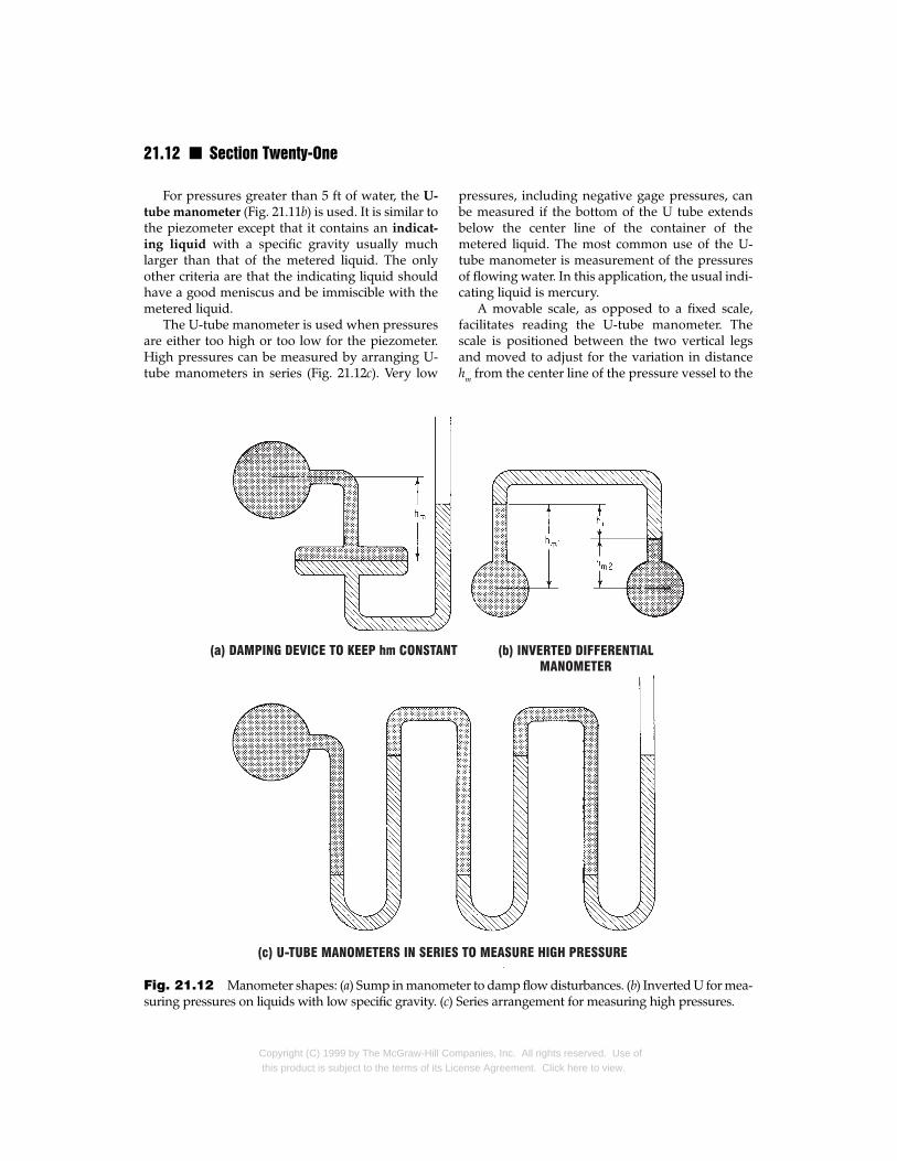
Fig. 21.12 Manometer shapes: (a) Sump in manomesuring pressures on liquids with low specific gravity. (c)
Copyright (C) 1999 by The McGraw-Hill Cothis product is subject to the terms of its Li
pressures, including negative gage pressures, canbe measured if the bottom of the U tube extendsbelow the center line of the container of themetered liquid. The most common use of the U-tube manometer is measurement of the pressuresof flowing water. In this application, the usual indi-cating liquid is mercury.
A movable scale, as opposed to a fixed scale,facilitates reading the U-tube manometer. Thescale is positioned between the two vertical legsand moved to adjust for the variation in distancehm from the center line of the pressure vessel to the
ter to damp flow disturbances. (b) Inverted U for mea- Series arrangement for measuring high pressures.
mpanies, Inc. All rights reserved. Use ofcense Agreement. Click here to view.
Water Resources Engineering n 21.13
indicating liquid. This zero adjustment enables adirect reading of the heights hi and hm of the liquidcolumns. The scale may be calibrated in any con-venient units, such as ft of water or psi.
The differential manometer (Fig. 21.11c) isidentical to the U-tube manometer but measuresthe difference in pressure between two points. (Itdoes not indicate the pressure at either point.) Thedifferential manometer may have either the stan-dard U-tube configuration or an inverted U-tubeconfiguration, depending on the comparative spe-cific gravities of the indicating and metered liq-uids. The inverted U-tube configuration (Fig.21.12b) is used when the indicating liquid has alower specific gravity than the metered liquid.
Example 21.4: A differential manometer (Fig.21.11c) is measuring the difference in pressurebetween two water pipes. The indicating liquid ismercury (specific gravity = 13.6), hi is 2.25 ft, hm1 is9 in, and z is 1.0 ft. What is the pressure differentialbetween the two pipes?
The pressure at B, psf, is
pB = pc2 + w2hm2 = pc2 + 62.4 × 2.0 = pc2 + 125
The pressure at A, psf, is
pA = pc1 + w1hm1 + wihi= pc1 + 62.4 × 0.75 + 13.6 × 62.4 × 2.25 = pc1 + 1957
Since the pressure at A must equal that at B,
pc2 + 125 = pc1 + 1957
Hence, the pressure differential between the pipes is
pc2 – pcl = 1832 psf = 12.7 psi
When small pressure differences in water aremeasured, if the specific gravity of the indicatingliquid is between 1.0 and 2.0 and the points atwhich the pressure is being measured are at thesame level, the actual pressure difference, whenexpressed in feet of water, is magnified by the dif-ferential manometer. For example, if the actual dif-ference is 0.50 ft of water and the indicating liquid
Copyright (C) 1999 by The McGraw-Hill Cothis product is subject to the terms of its Lic
has a specific gravity of 1.40, the magnification willbe 2.5; that is, the height of the liquid column hi willbe 1.25 ft of water. The closer the specific gravitiesof the metered and indicating liquids, the greaterthe magnification and sensitivity. This is true onlyup to a magnification of about 5. Above 5, theincreased sensitivity may be deceptive because themeniscus between the two liquids becomes poorlydefined and sluggish in movement.
Many factors affect the accuracy of manome-ters. Most of them, however, may be neglected inthe majority of hydraulics applications since theyare significant only in precise reading of manome-ters, such as might be required in laboratories. Onefactor, however, is significant: the existence ofsurges in the manometer caused by the pulsationsand disturbances in the flow of water resultingfrom turbulence. These surges make reading of themanometer difficult. They may be reduced or elim-inated by installing a large-diameter section, orsump, in the manometer, as shown in Fig. 21.12a.This sump will damp the pulsations and keep thedistance from the center line of the conduit to theindicating liquid essentially at a constant value.
21.6 Fundamentals of FluidFlow
For fluid energy, the law of conservation of energyis represented by the Bernoulli equation:
(21.11)
where Z1 = elevation, ft, at any point 1 of flow-ing fluid above an arbitrary datum
Z2 = elevation, ft, at downstream point influid above same datum
p1 = pressure at 1, psf
p2 = pressure at 2, psf
w = specific weight of fluid, lb/ft3
V1 = velocity of fluid at 1, ft/s
V2 = velocity of fluid at 2, ft/s
g = acceleration due to gravity, 32.2 ft/s2
The left side of the equation sums the total ener-gy per unit weight of fluid at 1, and the right side,the total energy per unit weight at 2. Equation
mpanies, Inc. All rights reserved. Use ofense Agreement. Click here to view.
21.14 n Section Twenty-One
(21.11) applies only to an ideal fluid. Its practical userequires a term to account for the decrease in totalhead, ft. through friction. This term hf, when addedto the downstream side of Eq. (21.11), yields theform of the Bernoulli equation most frequently used:
(21.12)
The energy contained in an elemental volumeof fluid thus is a function of its elevation, velocity,and pressure (Fig. 21.13). The energy due to eleva-tion is the potential energy and equals WZa, whereW is the weight, lb, of the fluid in the elementalvolume and Za is its elevation, ft, above some arbi-trary datum. The energy due to velocity is thekinetic energy. It equals WV 2
a / 2g, where Va is thevelocity, ft/s. The pressure energy equals Wpa /w,where pa is the pressure lb/ft2, and w is the specificweight of the fluid, lb/ft3. The total energy, in theelemental volume of fluid is
(21.13)
Dividing both sides of the equation by W yields theenergy per unit weight of flowing fluid, or the total
head ft:
(21.14)
pa/w is called pressure head; V2a/2g, velocity head.
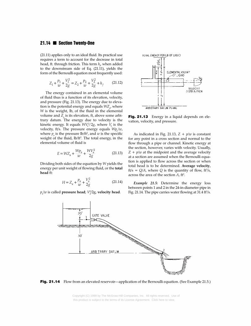
Fig. 21.14 Flow from an elevated reservoir—appli
Copyright (C) 1999 by The McGraw-Hill Cothis product is subject to the terms of its Li
As indicated in Fig. 21.13, Z + p/w is constantfor any point in a cross section and normal to theflow through a pipe or channel. Kinetic energy atthe section, however, varies with velocity. Usually,Z + p/w at the midpoint and the average velocityat a section are assumed when the Bernoulli equa-tion is applied to flow across the section or whentotal head is to be determined. Average velocity,ft/s = Q/A, where Q is the quantity of flow, ft3/s,across the area of the section A, ft2.
Example 21.5: Determine the energy lossbetween points 1 and 2 in the 24-in-diameter pipe inFig. 21.14. The pipe carries water flowing at 31.4 ft3/s.
Fig. 21.13 Energy in a liquid depends on ele-vation, velocity, and pressure.
cation of the Bernoulli equation. (See Example 21.5.)
mpanies, Inc. All rights reserved. Use ofcense Agreement. Click here to view.

Water Resources Engineering n 21.15
Fig. 21.15 Energy grade line and hydraulic grade line indicate variations in energy and pressurehead, respectively, in a liquid as it flows along a pipe or channel.
Average velocity in the pipe = Q/A = 31.4/ 3.14= 10 ft/s. Select point 1 far enough from the reser-voir outlet that V1 can be assumed to be 0. Since thedatum plane passes through point 2, Z2 = 0. Also,since the pipe has free discharge, p2 = 0. Thus sub-stitution in Eq. (21.12) yields
where hf is the friction loss, ft. Hence, hf = 50 – 1.55= 48.45 ft.
Note that in this example hf includes minor lossesdue to the pipe entrance, gate valve, and any bends.
The Bernoulli equation and the variation ofpressure may be represented graphically, respec-tively, by energy and hydraulic grade lines (Fig.21.15). The energy grade line, sometimes called thetotal head line, shows the decrease in total energyper unit weight H in the direction of flow. The slope
Copyright (C) 1999 by The McGraw-Hill Cothis product is subject to the terms of its L
of the energy grade line is called the energy gradi-
ent or friction slope. The hydraulic grade line lies adistance V2/2g below the energy grade line andshows the variation of velocity or pressure in thedirection of flow. The slope of the hydraulic gradeline is termed the hydraulic gradient. In open-channel flow, the hydraulic grade line coincideswith the water surface, while in pressure flow, itrepresents the height to which water would rise ina piezometer (see also Example 21.7, Art. 21.9).
Momentum is a fundamental concept that mustbe considered in the design of essentially all water-works facilities involving flow. A change in momen-tum, which may result from a change in eithervelocity, direction, or magnitude of flow, is equal tothe impulse, the force F acting on the fluid times theperiod of time dt over which it acts. Dividing thetotal change in momentum by the time intervalover which the change occurs gives the momentumequation, or impulse-momentum equation:
mpanies, Inc. All rights reserved. Use oficense Agreement. Click here to view.

21.16 n Section Twenty-One
(21.15)
where Fx = summation of all forces in X direc-tion per unit time causing change inmomentum in X direction, lb
ρ = density of flowing fluid, lb⋅s2/ft4
(specific weight divided by g)
Q = flow rate, ft3/s
∆Vx = change in velocity in X direction, ft/s
Similar equations may be written for the Y and Zdirections. The impulse-momentum equation oftenis used in conjunction with the Bernoulli equation[Eq. (21.11) or (21.12)] but may be used separately.
Example 21.6: Calculate the resultant force onthe reducer elbow in Fig. 21.16. The pipe centerline lies in a horizontal plane. The pipe reducesfrom 48 in in diameter to 16 in. The pressure at theupstream side of the reducer bend (point 1) is 100psi, and the water flow is 100 ft3/s. (Neglect frictionloss at the bend.)
Velocity at points 1 and 2 is found by dividingQ = 100 ft3/s by the respective areas: V1 = 100 ×4/42π = 7.96 ft/s and V2 = 100 × 4/1.332π = 71.5 ft/s.
With p1 known, the Bernoulli equation for theflow in the elbow is:
Fig. 21.16 Flow induces forces in a pipe at bendmomentum equation. (See Example 21.6.)
Copyright (C) 1999 by The McGraw-Hill Cothis product is subject to the terms of its L
Solution of the equation yields the pressure at 2:
p2 = 9500 psf
The total pressure force at 1 is P1 = p1A1 = 181,000lb, and at 2, P2 = ppA2 = 13,200 lb.
Let R be the force, lb, exerted by the pipe on thefluid (equal and opposite in direction to the forceagainst the pipe, which is to be determined). Then,the force F changing the momentum of the fluidequals the vector sum P1 – P2 + R. To find F, applyEq. (21.15) first in the X direction, then in the Ydirection, and determine the resultant of the forces:
In the X direction, since ∆Vx = –(7.96 sin 53.2° –71.5) = 65.1 and the density ρ = 62.4/ 32.2= 1.94,
Fx = 181,000 cos 53.2° – 13,200 + Rx= 1.94 × 100 × 65.1
Rx = –82,600 lb
In the Y direction, since ∆Vy = –(–7.96 cos 53.2° – 0)= 4.78,
Fy = –181,000 sin 53.2° + Ry = 1.94 × 100 × 4.78
Ry = 145,700 lb
The resultant R = √———Rx2+Ry
2— = 167,500 lb. It actsat an angle θ with the horizontal such that tan θ =145,700/82,600; so θ = 60.5°. The force against thepipe acts in the opposite direction.
s and at changes in size of section—application of
mpanies, Inc. All rights reserved. Use oficense Agreement. Click here to view.

Water Resources Engineering n 21.17
21.7 Water ResourcesModeling
A model is a tool that can be used to determine thelikely response of a system to a given set of stimuliwithout having to actually impose those stimuli onthe system. In water resources engineering, modelsare used to determine the likely response of a sys-tem, such as a river, aquifer, or drainage basin, to agiven set of stimuli, such as storm rainfall, droughts,alternative management schemes, or proposedworks. Models are cost-effective and convenient forsuch investigations. See also Art. 1.7.
Models can typically be categorized as one ofthree major types:
Physical Models n The system (prototype) ismodeled with physical components that representcomponents of the system. Usually, scale factorsare applied to set the model at only a fraction ofthe size and cost of the prototype. Physical modelsare expensive to build, operate, and maintain butare especially useful in analyzing complex phe-nomena that are not easy or presently possible toexpress mathematically.
Analog Models n The system (prototype) ismodeled with electronic circuits that representcomponents of the system. Some conveyance andresistance phenomena such as those found intransmission networks and groundwater analysesare easily modeled with analog techniques inas-much as electric current flow and water flowbehave similarly in certain instances. Analog mod-els are an abstraction of the prototype. Popularbefore the advent of digital computers, analogmodels are now infrequently used in view of theefficiency and portability of mathematical models.
Mathematical Models n The system (proto-type) is modeled with sets of mathematical expres-sions that represent components of the system.Mathematical models are normally programmed inan appropriate computer language, and throughexecution of the computer program, simulations ofprototype behavior are possible. Mathematicalmodels are limited only by the model creator’s abil-ity to describe the prototype mathematically, thecapability of the computing resources, or availabili-ty of data to support the modeling effort. They canbe as simple or as complex as a given analysis
Copyright (C) 1999 by The McGraw-Hill Cothis product is subject to the terms of its Lic
requires and are among the most cost-effectivemeans to perform certain analyses.
A fourth mode of modeling, hybrid modeling,employs both physical and mathematical models.It exploits the advantages of these types of modelswhile avoiding their limitations. For instance, com-plex three-dimensional flow patterns, erosionalscour, and sediment deposition occurring in theimmediate vicinity of a bridge pier or water controlstructure can be best modeled with a physicalmodel while the overall water surface, momen-tum, and velocity profile over the encompassingriver reach can be best modeled by an appropriatemathematical model.
With hybrid models, one model often providesinput to or verification of the other model. In thepreceding example, the mathematical modelwould provide depth and velocity profile input tothe physical model, and the physical model maybe able to provide a more accurate estimate of localhead loss at the pier or structure. In this way, thetwo models can be executed interactively until allcommon boundary conditions synchronize. Theresulting hybrid model will consist of a mathemat-ical model that properly accounts for overallhydraulic effects and local head loss at the pier orstructure and a physical model that properlyaccounts for localized forces affecting the stabilityor performance of the pier or structure.
21.7.1 Similitude for Physical Models
A physical model is a system whose operation canbe used to predict the characteristics of a similarsystem, or prototype, usually more complex orbuilt to a much larger scale. A knowledge of thelaws governing the phenomena under investiga-tion is necessary if the model study is to yield accu-rate quantitative results.
Forces acting on the model should be propor-tional to forces on the prototype. The four forcesusually considered in hydraulic models are inertia,gravity, viscosity, and surface tension. Because ofthe laws governing these forces and because themodel and prototype are normally not the samesize, it is usually not possible to have all four forcesin the model in the same proportions as they are inthe prototype. It is, however, a simple procedure tohave two predominant forces in the same propor-tion. In most models, the fact that two of the fourforces are not in the same proportion as they are in
mpanies, Inc. All rights reserved. Use ofense Agreement. Click here to view.

21.18 n Section Twenty-One
the prototype does not introduce serious error. Theinertial force, which is always a predominant force,and one other force are made proportional.
Ratios of the forces of gravity, viscosity, and sur-face tension to the force of inertia are designated,respectively, Froude number, Reynolds number,and Weber number. Equating the Froude numberof the model and the Froude number of the proto-type ensures that the gravitational and inertialforces are in the same proportion. Similarly, equat-ing the Reynolds numbers of the model and proto-type ensures that the viscous and inertial forceswill be in the same proportion. And equating theWeber numbers ensures proportionality of surfacetension and inertial forces.
The Froude number is
(21.16)
where F = Froude number (dimensionless)
V = velocity of fluid, ft/s
L = linear dimension (characteristic, suchas depth or diameter), ft
g = acceleration due to gravity, 32.2 ft/s2
For hydraulic structures, such as spillways andweirs, where there is a rapidly changing water-sur-face profile, the two predominant forces are inertiaand gravity. Therefore, the Froude numbers of themodel and prototype are equated:
(21.17a)
where subscript m applies to the model and p tothe prototype. Squaring both sides of Eq. (21.17a)and grouping like terms yields
(21.17b)
Let Vr = Vm/Vp and Lr = Lm/Lp. Then
(21.18)
The subscript r indicates ratio of quantity in modelto that in prototype.
If the ratios of all the physical dimensions of amodel to all the corresponding physical dimen-sions of the prototype are equal to the length ratio,
Copyright (C) 1999 by The McGraw-Hill Comthis product is subject to the terms of its Lic
the model is termed a true model. In a true modelwhere the Froude number is the governing designcriterion, the length ratio is the only variable. Oncethe length ratio has been set, all the physicaldimensions of the model are fixed. The dischargeratio is determined as follows:
(21.19a)
Since Vr = Lr1/2 and Ar = area ratio = L2
r ,
(21.19b)
By this method all the necessary characteristics of aspillway or weir model can be determined.
The Reynolds number is
(21.20)
R is dimensionless, and ν is the kinematic viscosityof fluid, ft2/s. The Reynolds numbers of model andprototype are equated when the viscous and inertialforces are predominant. Viscous forces are usuallypredominant when flow occurs in a closed system,such as pipe flow where there is no free surface. Thefollowing relations are obtained by equatingReynolds numbers of the model and prototype:
(21.21a)
(21.21b)
The variable factors that fix the design of a truemodel when the Reynolds number governs are thelength ratio and the viscosity ratio.
The Weber number is
(21.22)
where ρ = density of fluid, lb⋅s2/ft4 (specificweight divided by g)
σ = surface tension of fluid, psf
The Weber numbers of model and prototypeare equated in certain types of wave studies, theformation of drops and air bubbles, entrainment ofair in flowing water, and other phenomena wheresurface tension and inertial forces are predomi-nant. The velocity ratio is determined as follows:
panies, Inc. All rights reserved. Use ofense Agreement. Click here to view.

Water Resources Engineering n 21.19
(21.23a)
(21.23b)
The fluid properties and the length ratio fix thedesign of a model governed by the Weber number.
In some cases, such as a morning-glory spill-way, inertial, viscous, and gravity forces all have animportant effect on the flow. In these cases it isusually not possible to have both the Reynolds andFroude numbers of the model and prototypeequal. The solution to this type of problem is most-ly empirical and may consist of an attempt to eval-uate the effects of viscosity and gravity separately.
For the flow of water in open channels andrivers where the friction slope is relatively flat,model designs are often based on the Manningequation. The relations between the model andprototype are determined as follows:
(21.24)
where n = Manning roughness coefficient (T/L1/3,T representing time)
R = hydraulic radius (L)
S = loss of head due to friction per unitlength of conduit (dimensionless)
= slope of energy gradient
For true models, Sr = 1, Rr = Lr. Hence,
(21.25)
In models of rivers and channels, it is necessary forthe flow to be turbulent. The U.S. WaterwaysExperiment Station has determined that flow willbe turbulent if
(21.26)
where V = mean velocity, ft/s
R = hydraulic radius, ft
ν = kinematic viscosity, ft2/s
If the model is to be a true model, it may have to beuneconomically large for the flow to be turbulent.
Copyright (C) 1999 by The McGraw-Hill Cothis product is subject to the terms of its Lic
Another problem also encountered in true modelsis surface tension. In a true model of a wide riverwhere the depth may be only a fraction of an inch,the surface tension will distort the flow to such anextent that the model may be useless. To overcomethe effect of surface tension and to get turbulentflow, the depth scale is often made much largerthan the length scale. This type of model is called adistorted model.
The relations between a distorted model of achannel and a prototype are determined in thesame manner as was Eq. (21.24). The only differ-ence is that the slope ratio Sr equals the depth ratiodr and the hydraulic-radius ratio is a function of thewidth ratio and depth ratio.
One type of model, called a movable-bedmodel, is used to study erosion and transportationof silt in riverbeds. Because the laws governing thetransportation of material are not fully understood,movable-bed models are built largely on the basisof experience and give only qualitative results.
21.7.2 Types and Applications ofMathematical Models
Used in many applications of water resources engi-neering, mathematical models are, in particular,applied in hydrologic and hydraulic investigationsof man-made and natural systems for both surface-water and groundwater purposes. The system(prototype) is modeled with sets of mathematicalexpressions that represent components of the sys-tem. These expressions, in turn, are linked togeth-er to represent the system as a whole.
Mathematical models are used for both analysisand design. They are normally programmed in anappropriate computer language, and through exe-cution of the computer program, simulations ofprototype behavior are possible. They may be sin-gle-purpose (for a specific site) or general purpose(applicable to a variety of sites).
Single-purpose models typically represent thespecific temporal and spatial descriptions of theprototype directly in the computer code. Forinstance, the logical representation of prototypes,such as flow networks, catchment areas, and infil-tration parameters, may be part of the source codeand is said to be hardwired into the computer pro-gram. For such models, the software (the computerprogram code) and the application input codes(hydrologic and hydraulic parameters) are bound
mpanies, Inc. All rights reserved. Use ofense Agreement. Click here to view.

21.20 n Section Twenty-One
into one entity. This, however, usually has more dis-advantages than advantages, especially when mod-ifications of the model are required or when themodel has to be applied by engineers who were notinvolved in the original program coding. The pre-ferred approach in modeling is instead to developgeneral-purpose models by writing software that isessentially independent of application input code.
General-purpose models are used for specificanalytical tasks. These may be as simple as deter-mination of excess rainfall, given rainfall and rain-fall-loss parameters, or as complex as long-periodsimulation of flow and pollutant transport in com-bined groundwater and surface-water systems.
Advances are continually being made in com-puter resources and use of models is becomingmore widespread. As a result, the desirability ofmore uniformity of software packages and ofobject-oriented software has become apparent. Inobject-oriented software, every program compo-nent is generalized as much as feasible and theentire program is essentially a collection of modu-lar software components. This approach, whenfully implemented, will provide complete compat-ibility among all types of water resources software.Also, this approach will provide nearly completecompatibility of all databases, of all databases andsoftware, and among water resources modelers inthe government, academia, and private sectors.The result will be a reduction in duplication of theefforts of software developers and modelers andan increase in the efficiency of water-resourcesengineering investigations.
Typical applications of mathematical modelsinclude the following: stochastic processes; evapo-ration and irrigation; hydrodynamics; hydrologicforecasting; watershed hydrology; design ofhydraulic structures; reservoir regulation; flood ordrought impacts; flow routing; channel and riverhydraulics; sediment or pollutant transport; quan-tity and quality of water supply; ecosystemimpacts and restoration; impacts of dam breaks;wave or tidal analyses; landfill leachate analyses;and groundwater yield, seepage, or pollution.
Several different models varying in complexityor sophistication, or both, and in application typemay be required in many types of investigations.As a general rule, if comparisons of different plansare required, the fewer the number of modelsemployed in a given study, the greater the chancethat meaningful results will be produced. The
Copyright (C) 1999 by The McGraw-Hill Cothis product is subject to the terms of its L
availability and quality of data for calibration andverification, the model output required for designor evaluation, and the general acceptance by theengineering community should be considered inselection of a model or group of models for anyinvestigation.
Mathematical modeling is one of the fastestchanging fields in engineering. Applicationsshould be upgraded accordingly if their continueduse is expected.
(D. R. Maidment, “Handbook of Hydrology,” D.H. Hoggan, “Computer-Assisted FloodplainHydrology and Hydraulics,” N. S. Grigg, “WaterResources Planning,” V. J. Zipparo and H. Hasen,“Davis’ Handbook of Applied Hydraulics,”McGraw-Hill, New York.)
Pipe FlowThe term pipe flow as used in this section refers toflow in a circular closed conduit entirely filled withfluid. For closed conduits other than circular, rea-sonably good results are obtained in the turbulentrange with standard pipe-flow formulas if thediameter is replaced by four times the hydraulicradius. But when there is severe deviation from acircular cross section, as in annular passages, thismethod gives flows significantly underestimated.(J. F. Walker, G. A. Whan, and R. R. Rothfus, “FluidFriction in Noncircular Ducts,” Journal of the Ameri-can Institute of Chemical Engineers, vol. 3, 1957.)
21.8 Laminar FlowIn laminar flow, fluid particles move in parallel lay-ers in one direction. The parabolic velocity distrib-ution in laminar flow, shown in Fig. 21.17, creates ashearing stress τ = µ dV/dy, where dV/dy is the rateof change of velocity with depth and µ is the coef-ficient of viscosity (see Viscosity, Art. 21.2). As thisshearing stress increases, the viscous forcesbecome unable to damp out disturbances, and tur-bulent flow results. The region of change is depen-dent on the fluid’s velocity, density, and viscosityand the size of the conduit.
A dimensionless parameter called the Reynoldsnumber has been found to be a reliable criterionfor the determination of laminar or turbulent flow.It is the ratio of inertial forces to viscous forces, andis given by
mpanies, Inc. All rights reserved. Use oficense Agreement. Click here to view.

Water Resources Engineering n 21.21
(21.27)
where V = fluid velocity, ft/s
D = pipe diameter, ft
ρ = density of fluid, lb⋅s2/ft4 (specificweight divided by g, 32.2 ft/s2)
µ = viscosity of fluid lb⋅s/ft2
ν = µ/ρ = kinematic viscosity, ft2/s
For a Reynolds number less than 2000, flow is lam-inar in circular pipes. When the Reynolds numberis greater than 2000, laminar flow is unstable; a dis-turbance will probably be magnified, causing theflow to become turbulent.
In laminar flow, the following equation for headloss due to friction can be developed by consider-ing the forces acting on a cylinder of fluid in a pipe:
(21.28)
where hf = head loss due to friction, ft
L = length of pipe section considered, ft
g = acceleration due to gravity, 32.2 ft/s2
w = specific weight of fluid, lb/ft3
Substitution of the Reynolds number yields
(21.29)
For laminar flow, Eq. (21.29) is identical to theDarcy-Weisbach formula Eq. (21.30) since in lami-nar flow the friction f = 64 /R.
Fig. 21.17 Velocity distribution for lamellarflow in a circular pipe is parabolic. Maximum veloc-ity is twice the average velocity.
Copyright (C) 1999 by The McGraw-Hill Cothis product is subject to the terms of its Lic
(E. F. Brater, handbook of Hydraulics,” 6th ed.,McGraw-Hill Book Company, New York.)
21.9 Turbulent FlowIn turbulent flow, the inertial forces are so greatthat viscous forces cannot dampen out distur-bances caused primarily by the surface roughness.These disturbances create eddies, which have botha rotational and translational velocity. The transla-tion of these eddies is a mixing action that affectsan interchange of momentum across the cross sec-tion of the conduit. As a result, the velocity distrib-ution is more uniform, as shown in Fig. 21.18, thanfor laminar flow (Fig. 21.17).
For a Reynolds number greater than 2000 but tothe left of the dashed line in Fig. 21.l9, there is atransition from laminar to turbulent flow. In thisregion, there is a laminar film at the boundaries thatcovers some of the smaller roughness projections.This explains why the friction loss in this region hasboth laminar and turbulent characteristics. As theReynolds number increases, this laminar boundarylayer decreases in thickness until, at completely tur-bulent flow, it no longer covers any of the rough-ness projections. To the right of the dashed line inFig. 21.19, the flow is completely turbulent, and vis-cous forces do not affect the friction loss.
Because of the random nature of turbulentflow, it is not practical to treat it analytically. There-fore, formulas for head loss and flow in the turbu-lent regions have been developed through experi-mental and statistical means. Experimentation inturbulent flow has shown that:
The head loss varies directly as the length of the pipe.
The head loss varies almost as the square of thevelocity.
Fig. 21.18 Velocity distribution for turbulentflow in a circular pipe is more nearly uniform thanthat for lamellar flow.
mpanies, Inc. All rights reserved. Use ofense Agreement. Click here to view.

21.22 n Section Twenty-One
Fig. 21.19 Chart relates friction forces for flow in pipe to Reynolds numbers and condition of pipes.
The head loss varies almost inversely as the diameter.
The head loss depends on the surface roughness ofthe pipe wall.
The head loss depends on the fluid’s density andviscosity.
The head loss is independent of the pressure.
21.9.1 Darcy-Weisbach Formula
One of the most widely used equations for pipeflow, the Darcy-Weisbach formula satisfies theabove condition and is valid for laminar or turbu-lent flow in all fluids.
(21.30)
where hf = head loss due to friction, ft
f = friction factor (see Fig. 21.19)
L = length of pipe, ft
D = diameter of pipe, ft
V = velocity of fluid, ft/s
g = acceleration due to gravity, 32.2 ft/s2
Copyright (C) 1999 by The McGraw-Hill Cothis product is subject to the terms of its L
It employs the Moody diagram (Fig. 21.19) for eval-uating the friction factor f. (L. F. Moody, “FrictionFactors for Pipe Flow,” Transactions of the AmericanSociety of Mechanical Engineers, November 1944.)
Because Eq. (21.30) is dimensionally homoge-neous, it can be used with any consistent set of unitswithout changing the value of the friction factor.
ε, ft
Steel pipe:
Severe tuberculation and incrustation 0.03 – 0.008General tuberculation 0.008 – 0.003Heavy brush-coat asphalts, enamels,
and tars 0.003 – 0.001Light rust 0.001 – 0.0005New smooth pipe, centrifugally
applied enamels 0.0002 – 0.00003Hot-dipped asphalt; centrifugally
applied concrete linings 0.0005 – 0.0002Steel-formed concrete pipe, good
workmanship 0.0005 – 0.0002New cast-iron pipe 0.00085
Table 21.3 Typical Values of Roughness for Usein the Moody Diagram (Fig. 21.19) to Determine f
mpanies, Inc. All rights reserved. Use oficense Agreement. Click here to view.

Water Resources Engineering n 21.23
Roughness values ε (ft) for use with the Moodydiagram to determine the Darcy-Weisbach frictionfactor f are listed in Table 21.3.
The following formulas were derived for headloss in waterworks design and give good resultsfor water-transmission and -distribution calcula-tions. They contain a factor that depends on thesurface roughness of the pipe material. The accu-racy of these formulas is greatly affected by theselection of the roughness factor, which requiresexperience in its choice.
21.9.2 Chezy Formula
This equation holds for head loss in conduits andgives reasonably good results for high Reynoldsnumbers:
(21.31)
where V = velocity, ft/s
C = coefficient, dependent on surfaceroughness of conduit
S = slope of energy grade line or headloss due to friction, ft/ft of conduit
R = hydraulic radius, ft
Hydraulic radius of a conduit is the cross-sec-tional area of the fluid in it divided by the perime-ter of the wetted section.
21.9.3 Manning’s Formula
Through experimentation, Manning concludedthat the C in the Chezy equation [Eq. (21.31)]should vary as R1/6
(21.32)
where n = coefficient, dependent on surface rough-ness. (Although based on surface roughness, n inpractice is sometimes treated as a lumped parameterfor all head losses.) Substitution into Eq. (21.31) gives
(21.33a)
Upon substitution of D/4, where D is the pipediameter, for the hydraulic radius of the pipe, the fol-lowing equations are obtained for pipes flowing full:
Copyright (C) 1999 by The McGraw-Hill Cothis product is subject to the terms of its Lic
(21.33b)
(21.33c)
(21.33d)
(21.33e)
where Q = flow, ft3/s.Tables 21.4 and 21.11 (p. 21.47) give values of n
for the foot-pound-second system. See also Table22.3 for velocity and flow at various slopes.
21.9.4 Hazen-Williams Formula
This is one of the most widely used formulas forpipe-flow computations of water utilities, althoughit was developed for both open channels and pipeflow:
(21.34a)
For pipes flowing full:
(21.34b)
(21.34c)
(21.34d)
(21.34e)
where V = velocity, ft/s
C1 = coefficient, dependent on surfaceroughness
R = hydraulic radius, ft
S = head loss due to friction, ft/ft of pipe
D = diameter of pipe, ft
L = length of pipe, ft
mpanies, Inc. All rights reserved. Use ofense Agreement. Click here to view.
21.24 n Section Twenty-One
Variation Use in designingMaterial of pipe
From To From To
Clean cast iron 0.011 0.015 0.013 0.015Dirty or tuberculated cast iron 0.015 0.035Riveted steel or spiral steel 0.013 0.017 0.015 0.017Welded steel 0.010 0.013 0.012 0.013Galvanized iron 0.012 0.017 0.015 0.017Wood stave 0.010 0.014 0.012 0.013Concrete 0.010 0.017
Good workmanship 0.012 0.014Poor workmanship 0.016 0.017
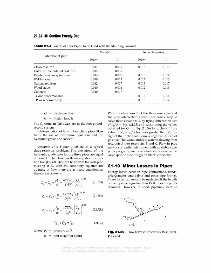
Table 21.4 Values of n for Pipes, to Be Used with the Manning Formula
Q = discharge, ft3/s
hf = friction loss, ft
The C1 terms in Table 21.5 are in the foot-pound-second system.
Determination of flow in branching pipes illus-trates the use of friction-loss equations and thehydraulic-grade-line concept.
Example 21.7: Figure 21.20 shows a typicalthree-reservoir problem. The elevations of thehydraulic grade lines for the three pipes are equalat point D. The Hazen-Williams equation for fric-tion loss [Eq. (21.34d)] can be written for each pipemeeting at D. With the continuity equation forquantity of flow, there are as many equations asthere are unknowns:
(21.35a)
(21.35b)
(21.35c)
(21.36)
where pD = pressure at D
w = unit weight of liquid
Copyright (C) 1999 by The McGraw-Hill Comthis product is subject to the terms of its Lic
With the elevations Z of the three reservoirs andthe pipe intersection known, the easiest way tosolve these equations is by trying different valuesof pD/w in Eqs. (21.35) and substituting the valuesobtained for Q into Eq. (21.36) for a check. If thevalue of Zd + pD/w becomes greater than Zb, thesign of the friction-loss term is negative instead ofpositive. This would indicate water is flowing fromreservoir A into reservoirs B and C. Flow in pipenetwork is easily determined with available com-puter programs, many of which are specialized tosolve specific pipe design problems efficiently.
21.10 Minor Losses in PipesEnergy losses occur in pipe contractions, bends,enlargements, and valves and other pipe fittings.These losses can usually be neglected if the lengthof the pipeline is greater than 1500 times the pipe’sdiameter. However, in short pipelines, because
Fig. 21.20 Flow between reservoirs. (See Exam-ple 21.7.)
panies, Inc. All rights reserved. Use ofense Agreement. Click here to view.

Water Resources Engineering n 21.25
these losses may exceed the friction losses, minorlosses must be considered.
21.10.1 Sudden Enlargements
The following equation for the head loss, ft, acrossa sudden enlargement of pipe diameter has beendetermined analytically and agrees well withexperimental results:
(21.37)
where V1 = velocity before enlargement, ft/s
V2 = velocity after enlargement, ft/s
g = 32.2 ft/s2
It was derived by applying the Bernoulli equationand the momentum equation across an enlargement.
Another equation for the head loss caused bysudden enlargements was determined experimental-ly by Archer. This equation gives slightly better agree-ment with experimental results than Eq. (21.37):
Type of pipe C1
Cast iron:New All sizes, 1305 years old All sizes up to 24 in, 120
24 in and over, 11510 years old 12 in, 110
4 in, 10530 in and over, 85
40 years old 16 in, 804 in, 65
Welded steel Values the same as for cast-ironpipe, 5 years older
Riveted steel Values the same as for cast-ironpipe, 10 years older
Wood stave Average value, regardless ofage, 120
Concrete or Large sizes, good workmanship,concrete-lined steel forms, 140
Large sizes, good workmanship,wood forms, 120
Centrifugally spun, 135
Vitrified In good condition, 110
Table 21.5 Values of C1 in Hazen and WilliamsFormula
Copyright (C) 1999 by The McGraw-Hill Cothis product is subject to the terms of its Lic
(21.38)
A special application of Eq. (21.37) or (21.38) is the dis-charge from a pipe into a reservoir. The water in thereservoir has no velocity, so a full velocity head is lost.
21.10.2 Gradual Enlargements
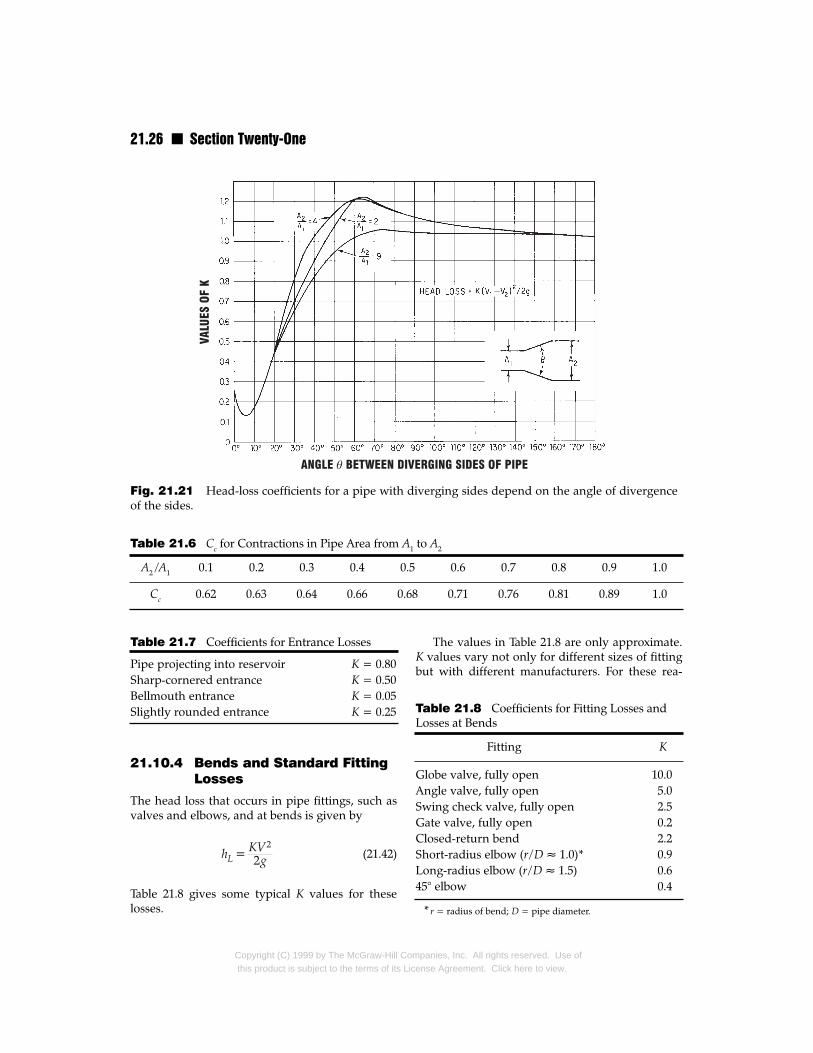
The equation for the head loss due to a gradual con-ical enlargement of a pipe takes the following form:
(21.39)
where K = loss coefficient (see Fig. 21.21).Since the experimental data available on grad-
ual enlargements are limited and inconclusive, thevalues of K in Fig. 21.21 are approximate. (A. H.Gibson, “Hydraulics and Its Applications,” Consta-ble & Co., Ltd., London.)
21.10.3 Sudden Contraction
The following equation for the head loss across asudden contraction of a pipe was determined bythe same type of analytical studies as Eq. (21.37):
(21.40)
where Cc = coefficient of contraction (see Table21.6)
V = velocity in smaller-diameter pipe, ft/s
This equation gives best results when the head lossis greater than 1 ft. Table 21.6 gives Cc values forsudden contractions, determined by Julius Weis-bach (“Die Experiments-Hydraulik”).
Another formula for determining the loss ofhead caused by a sudden contraction, determinedexperimentally by Brightmore, is
(21.41)
This equation gives best results if the head loss isless than 1 ft.
A special case of sudden contraction is theentrance loss for pipes. Some typical values ofthe loss coefficient K in hL = KV 2 / 2g, where V isthe velocity in the pipe, are presented in Table 21.7.
mpanies, Inc. All rights reserved. Use ofense Agreement. Click here to view.
21.26 n Section Twenty-One
Fig. 21.21 Head-loss coefficients for a pipe with diverging sides depend on the angle of divergenceof the sides.
A2 /A1 0.1 0.2 0.3 0.4 0.5 0.6 0.7 0.8 0.9 1.0
Cc 0.62 0.63 0.64 0.66 0.68 0.71 0.76 0.81 0.89 1.0
Table 21.6 Cc for Contractions in Pipe Area from A1 to A2
21.10.4 Bends and Standard FittingLosses
The head loss that occurs in pipe fittings, such asvalves and elbows, and at bends is given by
(21.42)
Table 21.8 gives some typical K values for theselosses.
Pipe projecting into reservoir K = 0.80Sharp-cornered entrance K = 0.50Bellmouth entrance K = 0.05Slightly rounded entrance K = 0.25
Table 21.7 Coefficients for Entrance Losses
Copyright (C) 1999 by The McGraw-Hill Cothis product is subject to the terms of its Lic
The values in Table 21.8 are only approximate.K values vary not only for different sizes of fittingbut with different manufacturers. For these rea-
Fitting K
Globe valve, fully open 10.0Angle valve, fully open 5.0Swing check valve, fully open 2.5Gate valve, fully open 0.2Closed-return bend 2.2Short-radius elbow (r /D ≈ 1.0)* 0.9Long-radius elbow (r /D ≈ 1.5) 0.645° elbow 0.4
*r = radius of bend; D = pipe diameter.
Table 21.8 Coefficients for Fitting Losses andLosses at Bends
mpanies, Inc. All rights reserved. Use ofense Agreement. Click here to view.

Water Resources Engineering n 21.27
sons, manufacturers’ data are the best source forloss coefficients.
Experimental data available on bend lossescover a rather narrow range of laboratory experi-ments utilizing small-diameter pipes and do notgive conclusive results. The data indicate the loss-es vary with surface roughness, Reynolds number,ratio of radius of bend r to pipe diameter D, andangle of bend. The data are in agreement that thehead loss, not including friction loss, decreasessharply as the r/D ratio increases from zero toaround 4 or 5. When r/D increases above 4 or 5,there is disagreement. Some experiments indicatethat the head loss, not including friction loss in thebend, increases significantly with an increasingr /D. Experiments on smooth pipes, indicate thatthis increase is very slight and that above an r/D of4, the bend loss essentially remains constant. (H.Ito, “Pressure Losses in Smooth Pipe Bends,” Trans-actions of the American Society of Civil Engineers,series D, vol. 82, no. 1, 1960.)
Because experiments have produced suchwidely varying data, bend-loss coefficients giveonly an approximation of losses to be expected.Figure 21.22 gives values of K for 90 ° bends for usewith Eq. (21.42). (K. H. Beij, “Pressure Losses forFluid Flow in 90° Pipe Bends,” Journal of Research,National Bureau of Standards, vol. 21, July 1938.)
To obtain losses in bends other than 90°, the fol-lowing formula may be used to adjust the K valuesgiven in Fig. 21.22:
(21.43)
where ∆ = deflection angle, degThe K′ value may be used in place of K in Eq.
(21.42).Minor losses are often given as the equivalent
length of pipe that has the same energy loss for thesame discharge. (V. J. Zipparo and H. Hasen,“Davis’ Handbook of Applied Hydraulics,” 4th ed.,McGraw-Hill, Inc., New York.)
21.11 OrificesAn orifice is an opening with a closed perimeterthrough which water flows. Orifices may have anyshape, although they are usually round, square, orrectangular.
Copyright (C) 1999 by The McGraw-Hill Comthis product is subject to the terms of its Lic
21.11.1 Orifice Discharge intoFree Air
Discharge through a sharp-edged orifice may becalculated from
(21.44)
where Q = discharge, ft3/s
C = coefficient of discharge
a = area of orifice, ft2
g = acceleration due to gravity, ft/s2
h = head on horizontal center line of ori-fice, ft
Coefficients of discharge C are given in Table21.9 for low velocity of approach. If this velocity issignificant, its effect should be taken into account.Equation (21.44) is applicable for any head forwhich the coefficient of discharge is known. Forlow heads, measuring the head from the centerline of the orifice is not theoretically correct; how-ever, this error is corrected by the C values.
The coefficient of discharge C is the product ofthe coefficient of velocity Cν and the coefficient ofcontraction Cc. The coefficient of velocity is theratio obtained by dividing the actual velocity at thevena contracta (contraction of the jet discharged)by the theoretical velocity. The theoretical velocitymay be calculated by writing Bernoulli’s equationfor points 1 and 2 in Fig. 21.23.
(21.45)
Fig. 21.22 Recommended values of head-losscoefficients K for 90° bends in closed conduits.
panies, Inc. All rights reserved. Use ofense Agreement. Click here to view.

21.28 n Section Twenty-One
Dia. of circular orifices, ft Side of square orifices, ft
0.02 0.04 0.1 1.0 0.02 0.04 0.1 1.0
0.637 0.618 0.4 0.643 0.6210.655 0.630 0.613 0.6 0.660 0.636 0.6170.648 0.626 0 610 0.590 0 8 0.652 0.631 0.615 0.5970.644 0.623 0.608 0.591 1 0.648 0.628 0.613 0.5990.637 0.618 0.605 0.593 1.5 0.641 0.622 0.610 0.601
0.632 0.614 0.604 0.595 2 0.637 0.619 0.608 0.6020.629 0.612 0.603 0.596 2.5 0.634 0.617 0.607 0.6020.627 0.611 0.603 0.597 3 0.632 0.616 0.607 0.6030.623 0.609 0.602 0.596 4 0.628 0.614 0.606 0.6020.618 0.607 0.600 0.596 6 0.623 0.612 0.605 0.602
0.614 0.605 0.600 0.596 8 0.619 0.610 0.605 0.6020.611 0.603 0.598 0.595 10 0.616 0.608 0.604 0.6010.601 0.599 0.596 0.594 20 0.606 0.604 0.602 0.6000.596 0.595 0.594 0.593 50 0.602 0.601 0.600 0.5990.593 0.592 0.592 0.592 100 0.599 0.598 0.598 0.598
*Hamilton Smith, Jr., “Hydraulics,” 1886.
Table 21.9 Smith’s Coefficients of Discharge for Circular and Square Orifices with Full Contraction*
Head,ft
With the reference plane through point 2, Z1 = h,V1 = 0, p1/w = p2/w = 0, and Z2 = 0, and Eq. (21.45)becomes
(21.46)
Fig. 21.23 Fluid jet
Copyright (C) 1999 by The McGraw-Hill Cothis product is subject to the terms of its L
The actual velocity, determined experimentally, isless than the theoretical velocity because of theenergy loss from point 1 to point 2. Typical valuesof Cν range from 0.94 to 0.99.
The coefficient of contraction Cc is the ratio ofthe smallest area of the jet, the vena contracta, to
takes a parabolic path.
mpanies, Inc. All rights reserved. Use oficense Agreement. Click here to view.
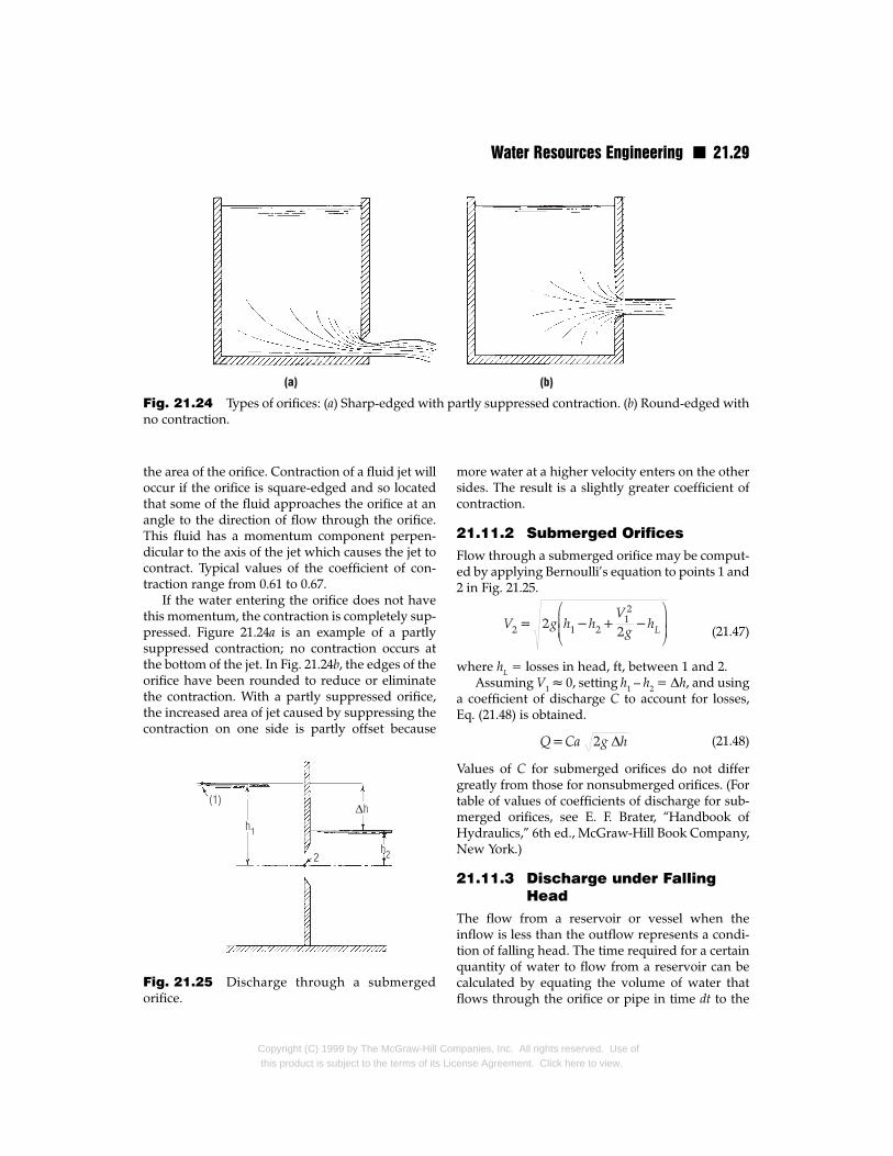
Water Resources Engineering n 21.29
Fig. 21.24 Types of orifices: (a) Sharp-edged with partly suppressed contraction. (b) Round-edged withno contraction.
the area of the orifice. Contraction of a fluid jet willoccur if the orifice is square-edged and so locatedthat some of the fluid approaches the orifice at anangle to the direction of flow through the orifice.This fluid has a momentum component perpen-dicular to the axis of the jet which causes the jet tocontract. Typical values of the coefficient of con-traction range from 0.61 to 0.67.
If the water entering the orifice does not havethis momentum, the contraction is completely sup-pressed. Figure 21.24a is an example of a partlysuppressed contraction; no contraction occurs atthe bottom of the jet. In Fig. 21.24b, the edges of theorifice have been rounded to reduce or eliminatethe contraction. With a partly suppressed orifice,the increased area of jet caused by suppressing thecontraction on one side is partly offset because
Fig. 21.25 Discharge through a submergedorifice.
Copyright (C) 1999 by The McGraw-Hill Cthis product is subject to the terms of its L
more water at a higher velocity enters on the othersides. The result is a slightly greater coefficient ofcontraction.
21.11.2 Submerged OrificesFlow through a submerged orifice may be comput-ed by applying Bernoulli’s equation to points 1 and2 in Fig. 21.25.
(21.47)
where hL = losses in head, ft, between 1 and 2.Assuming V1 ≈ 0, setting h1 – h2 = ∆h, and using
a coefficient of discharge C to account for losses,Eq. (21.48) is obtained.
(21.48)
Values of C for submerged orifices do not differgreatly from those for nonsubmerged orifices. (Fortable of values of coefficients of discharge for sub-merged orifices, see E. F. Brater, “Handbook ofHydraulics,” 6th ed., McGraw-Hill Book Company,New York.)
21.11.3 Discharge under FallingHead
The flow from a reservoir or vessel when theinflow is less than the outflow represents a condi-tion of falling head. The time required for a certainquantity of water to flow from a reservoir can becalculated by equating the volume of water thatflows through the orifice or pipe in time dt to the
ompanies, Inc. All rights reserved. Use oficense Agreement. Click here to view.

21.30 n Section Twenty-One
volume decrease in the reservoir (Fig. 21.26):
(21.49)
Solving for dt yields
(21.50)
where a = area of orifice, ft2
A = area of reservoir, ft2
y = head on orifice at time t, ft
C = coefficient of discharge
g = acceleration due to gravity, 32.2 ft/s2
Expressing the area as a function of y[A = F(y)] andsumming from time zero, when y = h1, to time t,when y = h2, Eq. (21.50) becomes
(21.51)
If the area of the reservoir is constant as y varies,Eq. (21.51) upon integration becomes
(21.52)
where h1 = head at the start, ft
h2 = head at the end, ft
t = time interval for head to fall from h1to h2, s
21.11.4 Fluid Jets
Where the effect of air resistance is small, a fluiddischarged through an orifice into the air will fol-low the path of a projectile. The initial velocity ofthe jet is
(21.53)
where h = head on center line of orifice, ft
Cν = coefficient of velocity
The direction of the initial velocity depends onthe orientation of the surface in which the orifice islocated. For simplicity, the following equationswere determined assuming the orifice is located ina vertical surface (Fig. 21.23). The velocity of the jetin the X direction (horizontal) remains constant.
Copyright (C) 1999 by The McGraw-Hill Comthis product is subject to the terms of its Lic
(21.54)
The velocity in the Y direction is initially zero andthereafter a function of time and the accelerationof gravity:
(21.55)
The X coordinate at time t is
(21.56)
The Y coordinate is
(21.57)
where Vavg = average velocity over period of timet. The equation for the path of the jet [Eq. (21.58)],obtained by solving Eq. (21.57) for t and substitut-ing in Eq. (21.56), is that for a parabola:
(21.58)
Equation (21.58) can be used to determine Cν
experimentally. Rearranging Eq. (21.58) gives
(21.59)
The X and Y coordinates can be measured in a lab-oratory and Cν calculated from Eq. (21.59).
Fig. 21.26 Discharge from a reservoir withdropping water level.
panies, Inc. All rights reserved. Use ofense Agreement. Click here to view.

Water Resources Engineering n 21.31
21.11.5 Orifice Discharge intoShort Tubes
When water flows from a reservoir into a pipe ortube with a sharp leading edge, the same type ofcontraction occurs as for a sharp-edged orifice. Inthe tube or pipe, however, the water contracts andthen expands to fill the tube. If the tube is dis-charging at atmospheric pressure, a partial vacu-um is created at the contraction, as can be seen byapplying the Bernoulli equation across points 1and 2 in Fig. 21.27. This reduced pressure causesthe flow through a short tube to be greater thanthat through a sharp-edged orifice of the samedimensions. If the head on the tube is greater than50 ft and the tube is short, the water will shootthrough the tube without filling it. When this hap-pens, the tube acts as a sharp-edged orifice.
For a short tube flowing full, the coefficient ofcontraction Cc = 1.00 and the coefficient of veloci-
Fig. 21.27 Flow from a reservoir through atube with a sharp-edged inlet.
Fig. 21.28 Flow from a reservoir through areentrant tube resembles that through a flush tube(Fig. 21.27) but the head loss is larger.
Copyright (C) 1999 by The McGraw-Hill Cothis product is subject to the terms of its Lic
ty Cν = 0.82. Therefore, the coefficient of dischargeC = 0.82. Solving for head loss as a proportion offinal velocity head, a K value for Eq. (21.42) of 0.5 isobtained as follows: The theoretical velocity headwith no loss is V2
T / 2g. Actual velocity head is V2a /2g
= (0.82 VT)2/2g = 0.67 V2T /2g. The head loss hL =
1.00 V 2T / 2g – 0.67 V 2
T / 2g = 0.33V 2T / 2g. From hL =
KV 2a / 2g, where V 2
a / 2g is the actual velocity head,
K = 2ghL/V2a = (0.33 V2
T × 2g)/(2g × 0.67 V2T) = 0.5
For a reentrant tube projecting into a reservoir(Fig. 21.28), the coefficients of velocity and dischargeequal 0.75, and the loss coefficient K equals 0.80.
21.11.6 Orifice Discharge intoDiverging Conical Tubes
This type of tube can greatly increase the flowthrough an orifice by reducing the pressure at theorifice below atmospheric. Equation (21.60) for thepressure at the entrance to the tube is obtained bywriting the Bernoulli equation for points 1 and 3and points 1 and 2 in Fig. 21.29.
(21.60)
where p2 = gage pressure at tube entrance, psf
w = unit weight of water, lb/ft3
h = head on center line of orifice, ft
a2 = area of smallest part of jet (vena con-tracta, if one exists), ft2
a3 = area of discharge end of tube, ft2
Fig. 21.29 Diverging conical tube increasesflow from a reservoir through an orifice by reduc-ing the pressure below atmospheric.
mpanies, Inc. All rights reserved. Use ofense Agreement. Click here to view.

21.32 n Section Twenty-One
Discharge is also calculated by writing theBernoulli equation for points 1 and 3 in Fig. 21.29.
For this analysis to be valid, the tube must flowfull, and the pressure in the throat of the tube mustnot fall to the vapor pressure of water. Experimentsby Venturi show the most efficient angle θ to bearound 5°.
21.12 SiphonsA siphon is a closed conduit that rises above thehydraulic grade line and in which the pressure atsome point is below atmospheric (Fig. 21.30). Themost common use of a siphon is the siphon spillway.
Flow through a siphon can be calculated bywriting the Bernoulli equation for the entranceand exit. But the pressure in the siphon must bechecked to be sure it does not fall to the vapor pres-sure of water. This is accomplished by writing theBernoulli equation across a point of known pres-sure and a point where the elevation head or thevelocity head is a maximum in the conduit. If thepressure were to fall to the vapor pressure, vapor-ization would decrease or totally stop the flow.
The pipe shown in Fig. 21.31 is also commonlycalled a siphon or inverted siphon. This is a mis-nomer since the pressure at all points in the pipe isabove atmospheric. The American Society of CivilEngineers recommends that the inverted siphonbe called a sag pipe to avoid the false impressionthat it acts as a siphon.
21.13 Water HammerWater hammer is a change in pressure, either aboveor below the normal pressure, caused by a variationof the flow rate in a pipe. Every time the flow rate is
Fig. 21.31 Sag pipe permits flow betwee
Copyright (C) 1999 by The McGraw-Hill Cothis product is subject to the terms of its Lic
changed, either increased or decreased, it causeswater hammer. However, the stresses are not criticalin small-diameter pipes with flows at low velocities.
The water flowing in a pipe has momentumequal to the mass of the water times its velocity.When a valve is closed, this momentum drops tozero. The change causes a pressure rise, whichbegins at the valve and is transmitted up the pipe.The pressure at the valve will rise until it is highenough to overcome the momentum of the waterand bring the water to a stop. This pressurebuildup travels the full length of the pipe to thereservoir (Fig. 21.32).
At the instant the pressure wave reaches thereservoir, the water in the pipe is motionless, but ata pressure much higher than normal. The differen-tial pressure between the pipe and the reservoirthen causes the water in the pipe to rush back intothe reservoir. As the water flows into the reservoir,the pressure in the pipe falls.
At the instant the pressure at the valve reachesnormal, the water has attained considerable momen-tum up the pipe. As the water flows away from theclosed valve, the pressure at the valve drops until dif-ferential pressure again brings the water to a stop.
Fig. 21.30 Siphon between reservoirs risesabove hydraulic grade line yet permits flow ofwater between them.
n two reservoirs despite a dip and a rise.
mpanies, Inc. All rights reserved. Use ofense Agreement. Click here to view.

Water Resources Engineering n 21.33
This pressure drop begins at the valve and continuesup the pipe until it reaches the reservoir.
The pressure in the pipe is now below normal,so water from the reservoir rushes into the pipe.This cycle repeats over and over until frictiondamps these oscillations. Because of the highvelocity of the pressure waves, each cycle may takeonly a fraction of a second.
The equation for the velocity of a wave in apipe is
(21.61)
where U = velocity of pressure wave along pipe,ft/s
E = modulus of elasticity of water, 43.2× 10⁶ psf
ρ = density of water, 1.94 lb⋅s/ft4 (specificweight divided by acceleration due togravity)
D = diameter of pipe, ft
Ep = modulus of elasticity of pipe material,psf
t = thickness of pipe wall, ft
21.13.1 Instantaneous Closure
The magnitude of the pressure change that resultswhen flow is varied depends on the rate of change
Fig. 21.32 Variation with time of pressure atthree points in a penstock, for water hammer frominstantaneous closure of a valve.
Copyright (C) 1999 by The McGraw-Hill Cothis product is subject to the terms of its Lic
of flow and the length of the pipeline. Any gradualmovement of a valve that is made in less time thanit takes for a pressure wave to travel from the valveto the reservoir and be reflected back to the valveproduces the same pressure change as an instanta-neous movement. For instantaneous closure:
(21.62)
where L = length of pipe from reservoir to valve,ft
T = time required to change setting ofvalve, s
A plot of pressure vs. time for various pointsalong a pipe is shown in Fig. 21.32 for the instanta-neous closure of a valve. Equation (21.63a) for thepressure rise or fall caused by adjusting a valvewas derived by equating the momentum of thewater in the pipe to the force impulse required tobring the water to a stop.
(21.63a)
In terms of pressure head, Eq. (21.63a) becomes
(21.63b)
where ∆p = pressure change from normal due toinstantaneous change of valve set-ting, psf
∆h = head change from normal due toinstantaneous change of valve set-ting, ft
∆V= change in the velocity of watercaused by adjusting valve, ft/s
If the closing or opening of a valve is instanta-neous, the pressure change can be calculated inone step from Eq. (21.63).
21.13.2 Gradual Closure
The following method of determining the pressurechange due to gradual closure of a valve gives aquick, approximate solution. The pressure rise orhead change is assumed to be in direct proportionto the closure time:
(21.64)
mpanies, Inc. All rights reserved. Use ofense Agreement. Click here to view.
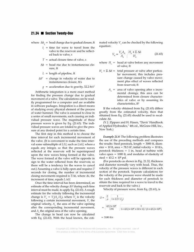
21.34 n Section Twenty-One
where ∆hg = head change due to gradual closure, ft
ti = time for wave to travel from thevalve to the reservoir and be reflect-ed back to valve, s
T = actual closure time of valve, s
∆h = head rise due to instantaneous clo-sure, ft
L = length of pipeline, ft
∆V = change in velocity of water due toinstantaneous closure, ft/s
g = acceleration due to gravity, 32.2 ft/s2
Arithmetic integration is a more exact methodfor finding the pressure change due to gradualmovement of a valve. The calculations can be read-ily programmed for a computer and are availablein software packages. Integration is a direct meansof studying every physical element of the processof water hammer. The valve is assumed to close ina series of small movements, each causing an indi-vidual pressure wave. The magnitude of thesepressure waves is given by Eq. (21.63). The indi-vidual pressure waves are totaled to give the pres-sure at any desired point for a certain time.
The first step in this method is to choose thetime interval for each incremental movement ofthe valve. (It is convenient to make the time inter-val some submultiple of L/U, such as L/aU, where aequals any integer, so that the pressure wavesreflected at the reservoir will be superimposedupon the new waves being formed at the valve.The wave formed at the valve will be opposite insign to the water reflected from the reservoir, sothere will be a tendency for the waves to cancelout.) Assuming a valve is fully open and requires Tseconds for closing, the number of incrementalclosing movements required is T/∆t, where ∆t, theincrement of time, equals L /aU.
Once the time interval has been determined, anestimate of the velocity change ∆V during each timeinterval must be made, to apply Eq. (21.63). A roughestimate for the velocity following the incrementalchange is Vn = Vo(An /Ao), where Vn is the velocityfollowing a certain incremental movement, Vo theoriginal velocity, An the area of the valve openingafter the corresponding incremental movement,and Ao the original area of the valve opening.
The change in head can now be calculatedwith Eq. (21.63). With the head known, the esti-
Copyright (C) 1999 by The McGraw-Hill Comthis product is subject to the terms of its Lic
mated velocity Vn can be checked by the followingequation:
(21.65)
where Ho = head at valve before any movementof valve, ft
Ho + Σ ∆h = total pressure at valve after particu-lar movement; this includes pres-sure change caused by valve move-ment plus effect of waves reflectedfrom reservoir, ft
An = area of valve opening after n incre-mental closings; this area can bedetermined from closure character-istics of valve or by assuming itscharacteristics, ft2
If the velocity obtained from Eq. (21.65) differsgreatly from the estimated velocity, then thatobtained from Eq. (21.65) should be used to recal-culate ∆h.
(V. J. Zipparo and H. Hasen, “Davis’ Handbookof Applied Hydraulics,” 4th ed., McGraw-Hill, Inc.,New York.)
Example 21.8: The following problem illustratesthe use of the preceding methods and comparesthe results: Steel penstock, length = 3000 ft, diam-eter = 10 ft, area = 78.5 ft2, initial velocity = 10 ft/s,penstock thickness = 1 in, head at turbine withvalve open = 1000 ft, and modulus of elasticity ofsteel = 43.2 × 10⁸ psf.
(For penstocks as shown in Fig. 21.32, thicknessand diameter normally vary with head. Thus, thevelocity of the pressure waves is different in eachsection of the penstock. Separate calculations forthe velocity of the pressure wave should be madefor each thickness and diameter of penstock toobtain the time required for a wave to travel to thereservoir and back to the valve.)
Velocity of pressure wave, from Eq. (21.61), is
= 3180 ft/s
panies, Inc. All rights reserved. Use ofense Agreement. Click here to view.

Water Resources Engineering n 21.35
The time required for the wave to travel to thereservoir and be reflected back to the valve = 2L/U= 6000/3180 = 1.90 s.
If closure time T of the valve is less than 1.90 s,the closure is instantaneous, and the pressure rise,from Eq. (21.63), is
Assuming T = 4.75 s, approximate equation(21.64) gives the following result:
21.13.3 Surge Tanks
It is uneconomical to design long pipelines forpressures created by water hammer or to operate avalve slowly enough to reduce these pressures.Usually, to prevent water hammer, a surge tank isinstalled close to valves at the end of long conduits.A surge tank is a tank containing water and con-nected to the conduit. The water column, in effect,floats on the line.
When a valve is suddenly closed, the water inthe line rushes into the surge tank. The water levelin the tank rises until the increased pressure in thesurge tank overcomes the momentum of the water.When a valve is suddenly opened, the surge tanksupplies water to the line when the pressuredrops. The section of pipe between the surge tankand the valve (Fig. 21.33) must still be designed forwater hammer; but the closure time to reduce thepressures for this section will be only a fraction ofthe time required without the surge tank.
Although a surge tank is one of the most com-monly used devices to prevent water hammer, it isby no means the only one. Various types of relief
Fig. 21.33 Surge tank is placed near a valve ona penstock to prevent water hammer.
Copyright (C) 1999 by The McGraw-Hill Cothis product is subject to the terms of its Lic
valves and air chambers are widely used on small-diameter lines, where the pressure of water ham-mer may be relieved by the release of a relativelysmall quantity of water.
Pipe Stresses
21.14 Pipe StressesPerpendicular to theLongitudinal Axis
The stresses acting perpendicular to the longitudi-nal axis of a pipe are caused by either internal orexternal pressures on the pipe walls.
Internal pressure creates a stress commonlycalled hoop tension. It may be calculated by taking afree-body diagram of a 1-in-long strip of pipe cut bya vertical plane through the longitudinal axis (Fig.21.34). The forces in the vertical direction cancel out.The sum of the forces in the horizontal direction is
(21.66)
where p = internal pressure, psi
D = outside diameter of pipe, in
F = force acting on each cut of edge ofpipe, lb
Hence, the stress, psi, on the pipe material is
(21.67)
where A = area of cut edge of pipe, ft2
t = thickness of pipe wall, in
Fig. 21.34 Internal pipe pressure produces hooptension.
mpanies, Inc. All rights reserved. Use ofense Agreement. Click here to view.

21.36 n Section Twenty-One
From the derivation of Eq. (21.67), it wouldappear that the diameter used for calculationsshould be the inside diameter. However, Eq. (21.67)is not theoretically exact and gives stresses slightlylower than those actually developed. For this reasonthe outside diameter often is used (see also Art. 6.10).
Equation (21.67) is exact for all practical purpos-es when D/t is equal to or greater than 50. If D/t isless than 10, this equation will usually be quite con-servative and therefore will yield an uneconomicaldesign. For steel pipes, Eq. (21.67) gives directly thethickness required to resist internal pressure.
For concrete pipes, this analysis is approximate,however, since concrete cannot resist large tensilestresses. The force F must be carried by steel rein-forcing. The internal diameter is used in Eq. (21.67)for concrete pipe.
When a pipe has external pressure acting on it,the analysis is much more complex because thepipe material no longer acts in direct tension. Theexternal pressure creates bending and compressivestresses that cause buckling.
(S. P. Timoshenko and J. M. Gere, “Theory ofelastic Stability,” 2nd ed., McGraw-Hill Book Com-pany, New York.)
21.15 Pipe Stresses Parallelto the Longitudinal Axis
If a pipe is supported on piers, it acts like a beam. Thestresses created can be calculated from the bendingmoment and shear equations for a continuous circu-lar hollow beam. This stress is usually not critical inhigh-head pipes. However, thin-walled pipes usual-ly require stiffening to prevent buckling and exces-sive deflection from the concentrated loads.
21.16 Temperature Expansionof Pipe
If a pipe is subject to a wide range of temperatures,the pipe should be the stress due to temperaturevariation designed for or expansion joints shouldbe provided. The stress, psi, due to a temperaturechange is
(21.68)
where E = modulus of elasticity of pipe material,psi
Copyright (C) 1999 by The McGraw-Hill Comthis product is subject to the terms of its Lic
∆T = temperature change from installationtemperature
c = coefficient of thermal expansion ofpipe material
The movement that should be allowed for, ifexpansion joints are to be used, is
(21.69)
where ∆L = movement in length L of pipe
L = length between expansion joints
21.17 Forces Due to PipeBends
It is common practice to use thrust blocks in pipebends to take the forces on the pipe caused by themomentum change and the unbalanced internalpressure of the water.
In all bends, there will be a slight loss of headdue to turbulence and friction. This loss will causea pressure change across the bend, but it is usuallysmall enough to be neglected. When there is achange in the cross-sectional area of the pipe, therewill be an additional pressure change that can becalculated with the Bernoulli equation (see Exam-ple 6, Art. 21.6). In this case, the pressure differen-tial may be large and must be considered.
The force diagram in Fig. 21.35 is a convenientmethod for finding the resultant force on a bend.The forces can be resolved into X and Y compo-nents to find the magnitude and direction of theresultant force on the pipe. In Fig. 21.35:
V1 = velocity before change in size ofpipe, ft/s
V2 = velocity after change in size of pipe,ft/s
p1 = pressure before bend or size changein pipe, psf
p2 = pressure after bend or size change inpipe, psf
A1 = area before size change in pipe, ft2
A2 = area after size change in pipe, ft2
F2m = force due to momentum of water insection 2 = V2Qw/g
F1m = force due to momentum of water insection 1 = V1Qw/g
panies, Inc. All rights reserved. Use ofense Agreement. Click here to view.

Water Resources Engineering n 21.37
Fig. 21.35 Forces produced by flow at a pipe bend and change in diameter.
P2 = pressure of water in section 2 timesarea of section 2 = p2A2
P1 = pressure of water in section 1 timesarea of section 1 = p1A1
w = unit weight of liquid, lb/ft3
Q = discharge, ft3/s
If the pressure loss in the bend is neglected and thereis no change in magnitude of velocity around thebend, Eqs. (21.70) and (21.71) give a quick solution.
(21.70)
(21.71)
where R = resultant force on bend, lb
α = angle R makes with F1m
p = pressure, psf
w = unit weight of water, 62.4 lb/ft3
V = velocity of flow, ft/s
g = acceleration due to gravity, 32.2 ft/s2
A = area of pipe, ft2
θ = angle between pipes (0° < θ < 180°)
Copyright (C) 1999 by The McGraw-Hill Cothis product is subject to the terms of its Lic
Although thrust blocks are normally used totake the force on bends, in many cases the pipematerial takes this force. The stress caused by thisforce is directly additive to other stresses alongthe longitudinal axis of the pipe. In small pipes,the force caused by bends can easily be carried bythe pipe material; however, the joints must alsobe able to take these forces.
CulvertsA culvert is a closed conduit for the passage of sur-face drainage under a highway, a railroad, canal, orother embankment. The slope of a culvert and itsinlet and outlet conditions are usually determinedby the topography of the site. Because of the manycombinations obtained by varying the entrance con-ditions, exit conditions, and slope, no single formulacan be given that will apply to all culvert problems.
The basic method for determining dischargethrough a culvert requires application of theBernoulli equation between a point just outsidethe entrance and a point somewhere downstream.An understanding of uniform and nonuniformflow is necessary to understand culvert flow fully.However, an exact theoretical analysis, involvingdetailed calculation of drawdown and backwatercurves, is usually unwarranted because of the rela-
mpanies, Inc. All rights reserved. Use ofense Agreement. Click here to view.
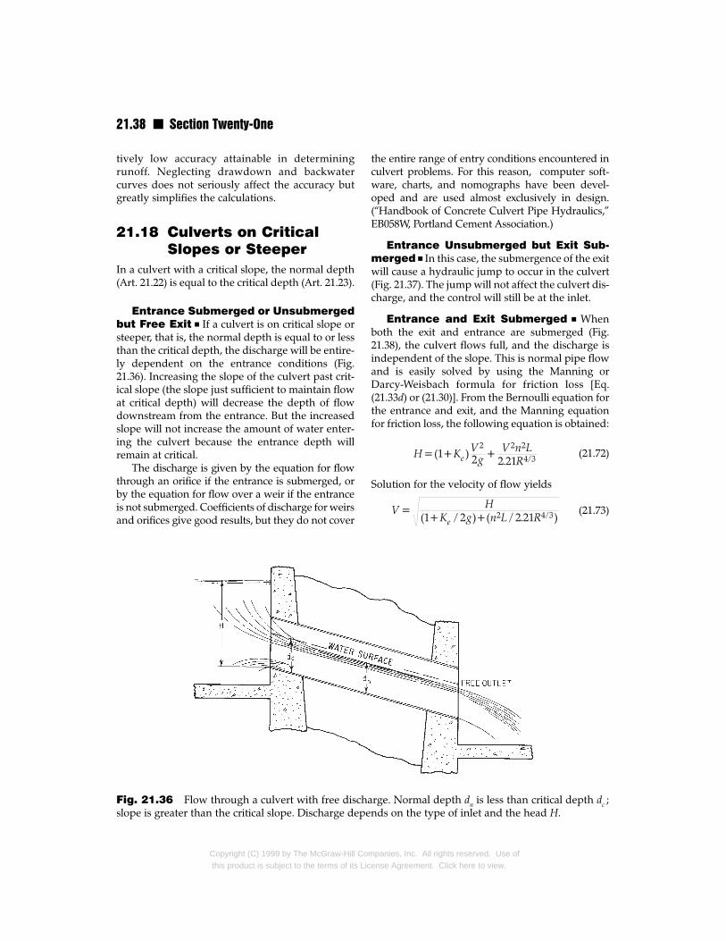
21.38 n Section Twenty-One
tively low accuracy attainable in determiningrunoff. Neglecting drawdown and backwatercurves does not seriously affect the accuracy butgreatly simplifies the calculations.
21.18 Culverts on CriticalSlopes or Steeper
In a culvert with a critical slope, the normal depth(Art. 21.22) is equal to the critical depth (Art. 21.23).
Entrance Submerged or Unsubmergedbut Free Exit n If a culvert is on critical slope orsteeper, that is, the normal depth is equal to or lessthan the critical depth, the discharge will be entire-ly dependent on the entrance conditions (Fig.21.36). Increasing the slope of the culvert past crit-ical slope (the slope just sufficient to maintain flowat critical depth) will decrease the depth of flowdownstream from the entrance. But the increasedslope will not increase the amount of water enter-ing the culvert because the entrance depth willremain at critical.
The discharge is given by the equation for flowthrough an orifice if the entrance is submerged, orby the equation for flow over a weir if the entranceis not submerged. Coefficients of discharge for weirsand orifices give good results, but they do not cover
Fig. 21.36 Flow through a culvert with free dischaslope is greater than the critical slope. Discharge depe
Copyright (C) 1999 by The McGraw-Hill Comthis product is subject to the terms of its Lic
the entire range of entry conditions encountered inculvert problems. For this reason, computer soft-ware, charts, and nomographs have been devel-oped and are used almost exclusively in design.(“Handbook of Concrete Culvert Pipe Hydraulics,”EB058W, Portland Cement Association.)
Entrance Unsubmerged but Exit Sub-merged n In this case, the submergence of the exitwill cause a hydraulic jump to occur in the culvert(Fig. 21.37). The jump will not affect the culvert dis-charge, and the control will still be at the inlet.
Entrance and Exit Submerged n Whenboth the exit and entrance are submerged (Fig.21.38), the culvert flows full, and the discharge isindependent of the slope. This is normal pipe flowand is easily solved by using the Manning orDarcy-Weisbach formula for friction loss [Eq.(21.33d) or (21.30)]. From the Bernoulli equation forthe entrance and exit, and the Manning equationfor friction loss, the following equation is obtained:
(21.72)
Solution for the velocity of flow yields
(21.73)
rge. Normal depth dn is less than critical depth dc ;nds on the type of inlet and the head H.
panies, Inc. All rights reserved. Use ofense Agreement. Click here to view.

Water Resources Engineering n 21.39
where H = elevation difference between head-water and tailwater, ft
V = velocity in culvert, ft/s
g = acceleration due to gravity, 32.2 ft/s2
Ke = entrance-loss coefficient (Art. 21.20)
n = Manning s roughness coefficient
L = length of culvert, ft
R = hydraulic radius of culvert, ft
Equation (21.72) can be solved directly since thevelocity is the only unknown.
21.19 Culverts on SubcriticalSlopes
Critical slope is the slope just sufficient to maintainflow at critical depth. When the slope is less thancritical, the flow is considered subcritical (Art. 21.23).
Entrance Submerged or Unsubmergedbut Free Exit n For these conditions, dependingon the head, the flow can be either pressure oropen-channel.
The discharge, for the open-channel condition(Fig. 21.39), is obtained by writing the Bernoulliequation for a point just outside the entrance anda point a short distance downstream from theentrance. Thus,
(21.74)
Fig. 21.37 Flow through a culvert with entranceunsubmerged but exit submerged. When slope isless than critical, open-channel flow takes place, anddn > dc . When slope exceeds critical, flow dependson inlet condition, and dn < dc .
Copyright (C) 1999 by The McGraw-Hill Cothis product is subject to the terms of its Lic
The velocity can be determined from the Man-ning equation:
(21.75)
Substituting this into Eq. (21.74) yields
(21.76)
where H = head on entrance measured from bot-tom of culvert, ft
Ke = entrance-loss coefficient (Art. 21.20)
Fig. 21.38 With entrance and exit of a culvertsubmerged, normal pipe flow occurs. Discharge isindependent of slope. The fluid flows under pres-sure. Discharge may be determined from Bernoulliand Manning equations.
Fig. 21.39 Open-channel flow occurs in a cul-vert with free discharge and normal depth dngreater than the critical depth dc when the entranceis unsubmerged or slightly submerged. Dischargedepends on head H, loss at entrance, and slope ofculvert.
mpanies, Inc. All rights reserved. Use ofense Agreement. Click here to view.
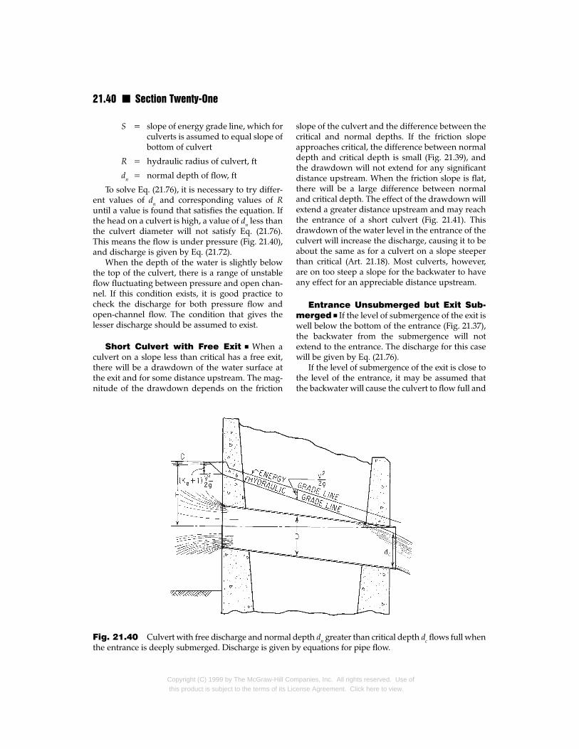
21.40 n Section Twenty-One
S = slope of energy grade line, which forculverts is assumed to equal slope ofbottom of culvert
R = hydraulic radius of culvert, ft
dn = normal depth of flow, ft
To solve Eq. (21.76), it is necessary to try differ-ent values of dn and corresponding values of Runtil a value is found that satisfies the equation. Ifthe head on a culvert is high, a value of dn less thanthe culvert diameter will not satisfy Eq. (21.76).This means the flow is under pressure (Fig. 21.40),and discharge is given by Eq. (21.72).
When the depth of the water is slightly belowthe top of the culvert, there is a range of unstableflow fluctuating between pressure and open chan-nel. If this condition exists, it is good practice tocheck the discharge for both pressure flow andopen-channel flow. The condition that gives thelesser discharge should be assumed to exist.
Short Culvert with Free Exit n When aculvert on a slope less than critical has a free exit,there will be a drawdown of the water surface atthe exit and for some distance upstream. The mag-nitude of the drawdown depends on the friction
Fig. 21.40 Culvert with free discharge and normal dthe entrance is deeply submerged. Discharge is given b
Copyright (C) 1999 by The McGraw-Hill Cothis product is subject to the terms of its Lic
slope of the culvert and the difference between thecritical and normal depths. If the friction slopeapproaches critical, the difference between normaldepth and critical depth is small (Fig. 21.39), andthe drawdown will not extend for any significantdistance upstream. When the friction slope is flat,there will be a large difference between normaland critical depth. The effect of the drawdown willextend a greater distance upstream and may reachthe entrance of a short culvert (Fig. 21.41). Thisdrawdown of the water level in the entrance of theculvert will increase the discharge, causing it to beabout the same as for a culvert on a slope steeperthan critical (Art. 21.18). Most culverts, however,are on too steep a slope for the backwater to haveany effect for an appreciable distance upstream.
Entrance Unsubmerged but Exit Sub-merged n If the level of submergence of the exit iswell below the bottom of the entrance (Fig. 21.37),the backwater from the submergence will notextend to the entrance. The discharge for this casewill be given by Eq. (21.76).
If the level of submergence of the exit is close tothe level of the entrance, it may be assumed thatthe backwater will cause the culvert to flow full and
epth dn greater than critical depth dc flows full wheny equations for pipe flow.
mpanies, Inc. All rights reserved. Use ofense Agreement. Click here to view.
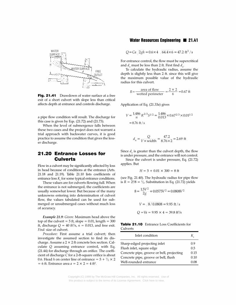
Water Resources Engineering n 21.41
a pipe flow condition will result. The discharge forthis case is given by Eqs. (21.72) and (21.73).
When the level of submergence falls betweenthese two cases and the project does not warrant atrial approach with backwater curves, it is goodpractice to assume the condition that gives the less-er discharge.
21.20 Entrance Losses forCulverts
Flow in a culvert may be significantly affected by lossin head because of conditions at the entrance (Arts.21.18 and 21.19). Table 21.10 lists coefficients ofentrance loss Ke for some typical entrance conditions.
These values are for culverts flowing full. Whenthe entrance is not submerged, the coefficients areusually somewhat lower. But because of the manyunknowns entering into determination of culvertflow, the values tabulated can be used for sub-merged or unsubmerged cases without much lossof accuracy.
Example 21.9: Given: Maximum head above thetop of the culvert = 5 ft, slope = 0.01, length = 300ft, discharge Q = 40 ft3/s, n = 0.013, and free exit.Find: size of culvert.
Procedure: First assume a trial culvert; theninvestigate the assumed section to find its dis-charge. Assume a 2 × 2 ft concrete box section. Cal-culate Q assuming entrance control, with Eq.(21.44) for discharge through an orifice. The coeffi-cient of discharge C for a 2-ft-square orifice is about0.6. Head h on center line of entrance = 5 + 1/2 × 2= 6 ft. Entrance area a = 2 × 2 = 4 ft2.
Fig. 21.41 Drawdown of water surface at a freeexit of a short culvert with slope less than criticalaffects depth at entrance and controls discharge.
Copyright (C) 1999 by The McGraw-Hill Cothis product is subject to the terms of its Lic
For entrance control, the flow must be supercriticaland dn must be less than 2 ft. First find dn.
To calculate the hydraulic radius, assume thedepth is slightly less than 2 ft. since this will givethe maximum possible value of the hydraulicradius for this culvert.
Application of Eq. (21.33a) gives
Since dn is greater than the culvert depth, the flowis under pressure, and the entrance will not control.
Since the culvert is under pressure, Eq. (21.72)applies. But
H = 5 + 0.01 × 300 = 8 ft
(see Fig. 21.40). The hydraulic radius for pipe flowis R = 22/8 = 1/2. Substitution in Eq. (21.72) yields
Q =Va = 9.95 × 4 = 39.8 ft3/s
Inlet condition Ke
Sharp-edged projecting inlet 0.9Flush inlet, square edge 0.5Concrete pipe, groove or bell, projecting 0.15Concrete pipe, groove or bell, flush 0.10Well-rounded entrance 0.08
Table 21.10 Entrance Loss Coefficients forCulverts
mpanies, Inc. All rights reserved. Use ofense Agreement. Click here to view.
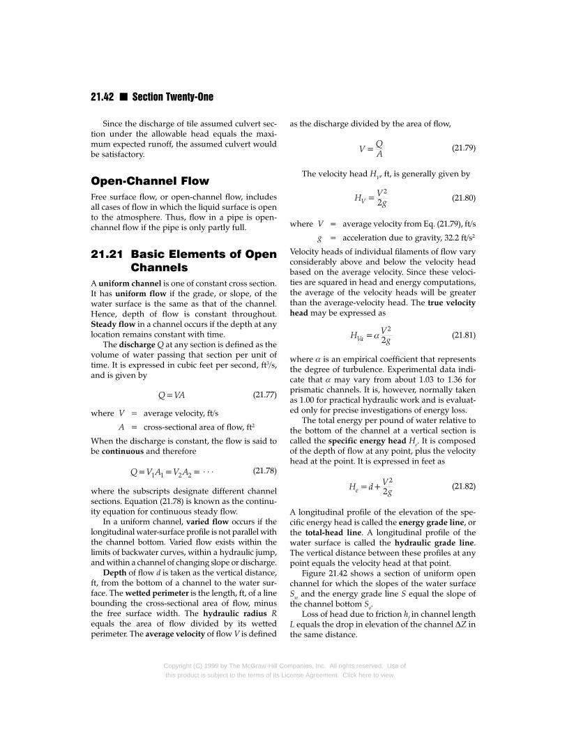
21.42 n Section Twenty-One
Since the discharge of tile assumed culvert sec-tion under the allowable head equals the maxi-mum expected runoff, the assumed culvert wouldbe satisfactory.
Open-Channel FlowFree surface flow, or open-channel flow, includesall cases of flow in which the liquid surface is opento the atmosphere. Thus, flow in a pipe is open-channel flow if the pipe is only partly full.
21.21 Basic Elements of OpenChannels
A uniform channel is one of constant cross section.It has uniform flow if the grade, or slope, of thewater surface is the same as that of the channel.Hence, depth of flow is constant throughout.Steady flow in a channel occurs if the depth at anylocation remains constant with time.
The discharge Q at any section is defined as thevolume of water passing that section per unit oftime. It is expressed in cubic feet per second, ft3/s,and is given by
(21.77)
where V = average velocity, ft/s
A = cross-sectional area of flow, ft2
When the discharge is constant, the flow is said tobe continuous and therefore
(21.78)
where the subscripts designate different channelsections. Equation (21.78) is known as the continu-ity equation for continuous steady flow.
In a uniform channel, varied flow occurs if thelongitudinal water-surface profile is not parallel withthe channel bottom. Varied flow exists within thelimits of backwater curves, within a hydraulic jump,and within a channel of changing slope or discharge.
Depth of flow d is taken as the vertical distance,ft, from the bottom of a channel to the water sur-face. The wetted perimeter is the length, ft, of a linebounding the cross-sectional area of flow, minusthe free surface width. The hydraulic radius Requals the area of flow divided by its wettedperimeter. The average velocity of flow V is defined
Copyright (C) 1999 by The McGraw-Hill Comthis product is subject to the terms of its Lic
as the discharge divided by the area of flow,
(21.79)
The velocity head HV, ft, is generally given by
(21.80)
where V = average velocity from Eq. (21.79), ft/s
g = acceleration due to gravity, 32.2 ft/s2
Velocity heads of individual filaments of flow varyconsiderably above and below the velocity headbased on the average velocity. Since these veloci-ties are squared in head and energy computations,the average of the velocity heads will be greaterthan the average-velocity head. The true velocity
head may be expressed as
(21.81)
where α is an empirical coefficient that representsthe degree of turbulence. Experimental data indi-cate that α may vary from about 1.03 to 1.36 forprismatic channels. It is, however, normally takenas 1.00 for practical hydraulic work and is evaluat-ed only for precise investigations of energy loss.
The total energy per pound of water relative tothe bottom of the channel at a vertical section iscalled the specific energy head He. It is composedof the depth of flow at any point, plus the velocityhead at the point. It is expressed in feet as
(21.82)
A longitudinal profile of the elevation of the spe-cific energy head is called the energy grade line, orthe total-head line. A longitudinal profile of thewater surface is called the hydraulic grade line.The vertical distance between these profiles at anypoint equals the velocity head at that point.
Figure 21.42 shows a section of uniform openchannel for which the slopes of the water surfaceSw and the energy grade line S equal the slope ofthe channel bottom So.
Loss of head due to friction hf in channel lengthL equals the drop in elevation of the channel ∆Z inthe same distance.
panies, Inc. All rights reserved. Use ofense Agreement. Click here to view.
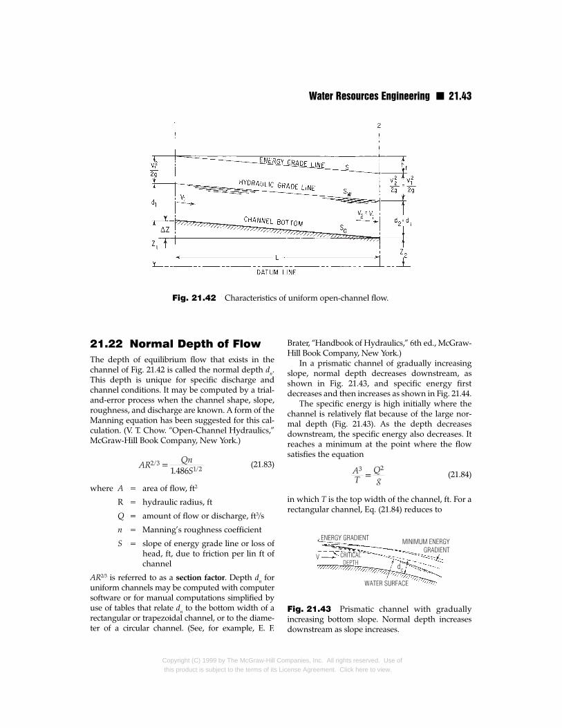
Water Resources Engineering n 21.43
Fig. 21.42 Characteristics of uniform open-channel flow.
21.22 Normal Depth of FlowThe depth of equilibrium flow that exists in thechannel of Fig. 21.42 is called the normal depth dn.This depth is unique for specific discharge andchannel conditions. It may be computed by a trial-and-error process when the channel shape, slope,roughness, and discharge are known. A form of theManning equation has been suggested for this cal-culation. (V. T. Chow. “Open-Channel Hydraulics,”McGraw-Hill Book Company, New York.)
(21.83)
where A = area of flow, ft2
R = hydraulic radius, ft
Q = amount of flow or discharge, ft3/s
n = Manning’s roughness coefficient
S = slope of energy grade line or loss ofhead, ft, due to friction per lin ft ofchannel
AR2/3 is referred to as a section factor. Depth dn foruniform channels may be computed with computersoftware or for manual computations simplified byuse of tables that relate dn to the bottom width of arectangular or trapezoidal channel, or to the diame-ter of a circular channel. (See, for example, E. F.
Copyright (C) 1999 by The McGraw-Hill Comthis product is subject to the terms of its Lic
Brater, “Handbook of Hydraulics,” 6th ed., McGraw-Hill Book Company, New York.)
In a prismatic channel of gradually increasingslope, normal depth decreases downstream, asshown in Fig. 21.43, and specific energy firstdecreases and then increases as shown in Fig. 21.44.
The specific energy is high initially where thechannel is relatively flat because of the large nor-mal depth (Fig. 21.43). As the depth decreasesdownstream, the specific energy also decreases. Itreaches a minimum at the point where the flowsatisfies the equation
(21.84)
in which T is the top width of the channel, ft. For arectangular channel, Eq. (21.84) reduces to
Fig. 21.43 Prismatic channel with graduallyincreasing bottom slope. Normal depth increasesdownstream as slope increases.
panies, Inc. All rights reserved. Use ofense Agreement. Click here to view.

21.44 n Section Twenty-One
Fig. 21.44 Specific energy head He changes with depth for constant discharge in a rectangular channelof changing slope. He is a minimum for flow with critical depth.
(21.85)
where V = Q/A = mean velocity of flow, ft3/s
d = depth of flow, ft
This indicates that the specific energy is a minimumwhere the normal depth equals twice the velocityhead. As the depth continues to decrease in thedownstream direction, the specific energy increasesagain because of the higher velocity head (Fig. 21.44).
21.23 Critical Depth of Open-Channel Flow
The depth of flow that satisfies Eq. (21.84) is calledthe critical depth dc. For a given value of specificenergy, the critical depth gives the greatest dis-charge, or conversely, for a given discharge, thespecific energy is a minimum for the critical depth(Fig. 21.44).
Copyright (C) 1999 by The McGraw-Hill Cothis product is subject to the terms of its Li
In the section of mild slope upstream from thecritical-depth point in Fig 21.43, the depth isgreater than critical. The flow there is called sub-
critical flow, indicating that the velocity is lessthan that at critical depth. In the section of steeperslope below the critical-depth point, the depth isbelow critical. The velocity there exceeds that atcritical depth, and flow is supercritical.
Critical depth may be computed for a uniformchannel once the discharge is known. Determina-tion of this depth is independent of the channelslope and roughness since critical depth simply rep-resents a depth for which the specific energy headis a minimum. Critical depth may be calculated bytrial and error with Eq. (21.84), or it may be founddirectly from tables (E. F. Brater, “Handbook ofHydraulics,” 6th ed., McGraw-Hill Book Company,New York). For rectangular channels, Eq. (21.84)may be reduced to
(21.86)
mpanies, Inc. All rights reserved. Use ofcense Agreement. Click here to view.
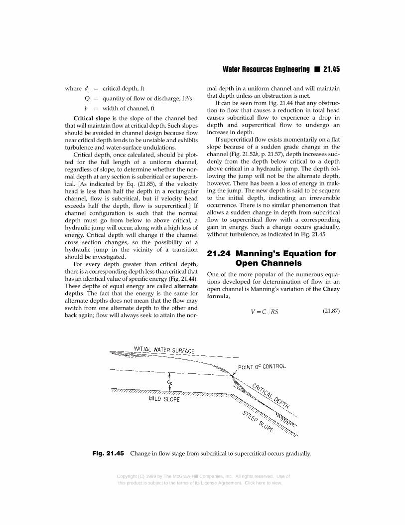
Water Resources Engineering n 21.45
where dc = critical depth, ft
Q = quantity of flow or discharge, ft3/s
b = width of channel, ft
Critical slope is the slope of the channel bedthat will maintain flow at critical depth. Such slopesshould be avoided in channel design because flownear critical depth tends to be unstable and exhibitsturbulence and water-surface undulations.
Critical depth, once calculated, should be plot-ted for the full length of a uniform channel,regardless of slope, to determine whether the nor-mal depth at any section is subcritical or supercrit-ical. [As indicated by Eq. (21.85), if the velocityhead is less than half the depth in a rectangularchannel, flow is subcritical, but if velocity headexceeds half the depth, flow is supercritical.] Ifchannel configuration is such that the normaldepth must go from below to above critical, ahydraulic jump will occur, along with a high loss ofenergy. Critical depth will change if the channelcross section changes, so the possibility of ahydraulic jump in the vicinity of a transitionshould be investigated.
For every depth greater than critical depth,there is a corresponding depth less than critical thathas an identical value of specific energy (Fig. 21.44).These depths of equal energy are called alternate
depths. The fact that the energy is the same foralternate depths does not mean that the flow mayswitch from one alternate depth to the other andback again; flow will always seek to attain the nor-
Fig. 21.45 Change in flow stage from su
Copyright (C) 1999 by The McGraw-Hill Cothis product is subject to the terms of its Lic
mal depth in a uniform channel and will maintainthat depth unless an obstruction is met.
It can be seen from Fig. 21.44 that any obstruc-tion to flow that causes a reduction in total headcauses subcritical flow to experience a drop indepth and supercritical flow to undergo anincrease in depth.
If supercritical flow exists momentarily on a flatslope because of a sudden grade change in thechannel (Fig. 21.52b, p. 21.57), depth increases sud-denly from the depth below critical to a depthabove critical in a hydraulic jump. The depth fol-lowing the jump will not be the alternate depth,however. There has been a loss of energy in mak-ing the jump. The new depth is said to be sequentto the initial depth, indicating an irreversibleoccurrence. There is no similar phenomenon thatallows a sudden change in depth from subcriticalflow to supercritical flow with a correspondinggain in energy. Such a change occurs gradually,without turbulence, as indicated in Fig. 21.45.
21.24 Manning’s Equation forOpen Channels
One of the more popular of the numerous equa-tions developed for determination of flow in anopen channel is Manning’s variation of the Chezy
formula,
(21.87)
bcritical to supercritical occurs gradually.
mpanies, Inc. All rights reserved. Use ofense Agreement. Click here to view.
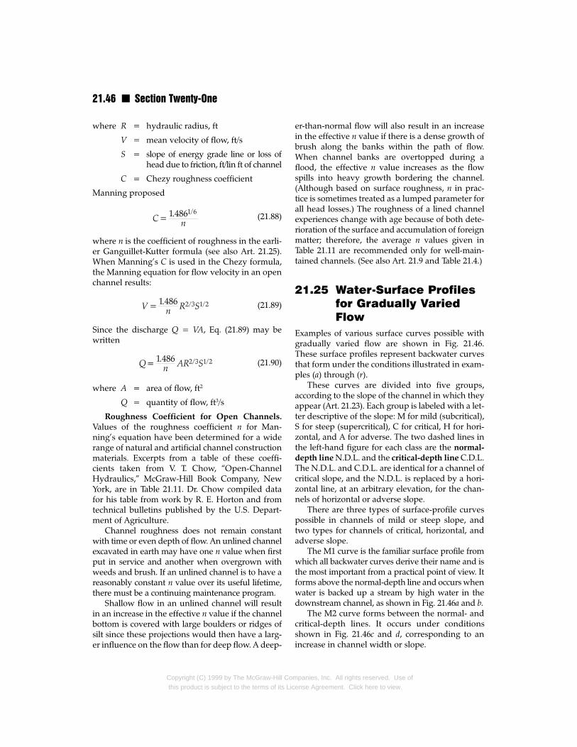
21.46 n Section Twenty-One
where R = hydraulic radius, ft
V = mean velocity of flow, ft/s
S = slope of energy grade line or loss ofhead due to friction, ft/lin ft of channel
C = Chezy roughness coefficient
Manning proposed
(21.88)
where n is the coefficient of roughness in the earli-er Ganguillet-Kutter formula (see also Art. 21.25).When Manning’s C is used in the Chezy formula,the Manning equation for flow velocity in an openchannel results:
(21.89)
Since the discharge Q = VA, Eq. (21.89) may bewritten
(21.90)
where A = area of flow, ft2
Q = quantity of flow, ft3/s
Roughness Coefficient for Open Channels.
Values of the roughness coefficient n for Man-ning’s equation have been determined for a widerange of natural and artificial channel constructionmaterials. Excerpts from a table of these coeffi-cients taken from V. T. Chow, “Open-ChannelHydraulics,” McGraw-Hill Book Company, NewYork, are in Table 21.11. Dr. Chow compiled datafor his table from work by R. E. Horton and fromtechnical bulletins published by the U.S. Depart-ment of Agriculture.
Channel roughness does not remain constantwith time or even depth of flow. An unlined channelexcavated in earth may have one n value when firstput in service and another when overgrown withweeds and brush. If an unlined channel is to have areasonably constant n value over its useful lifetime,there must be a continuing maintenance program.
Shallow flow in an unlined channel will resultin an increase in the effective n value if the channelbottom is covered with large boulders or ridges ofsilt since these projections would then have a larg-er influence on the flow than for deep flow. A deep-
Copyright (C) 1999 by The McGraw-Hill Comthis product is subject to the terms of its Lic
er-than-normal flow will also result in an increasein the effective n value if there is a dense growth ofbrush along the banks within the path of flow.When channel banks are overtopped during aflood, the effective n value increases as the flowspills into heavy growth bordering the channel.(Although based on surface roughness, n in prac-tice is sometimes treated as a lumped parameter forall head losses.) The roughness of a lined channelexperiences change with age because of both dete-rioration of the surface and accumulation of foreignmatter; therefore, the average n values given inTable 21.11 are recommended only for well-main-tained channels. (See also Art. 21.9 and Table 21.4.)
21.25 Water-Surface Profilesfor Gradually VariedFlow
Examples of various surface curves possible withgradually varied flow are shown in Fig. 21.46.These surface profiles represent backwater curvesthat form under the conditions illustrated in exam-ples (a) through (r).
These curves are divided into five groups,according to the slope of the channel in which theyappear (Art. 21.23). Each group is labeled with a let-ter descriptive of the slope: M for mild (subcritical),S for steep (supercritical), C for critical, H for hori-zontal, and A for adverse. The two dashed lines inthe left-hand figure for each class are the normal-
depth line N.D.L. and the critical-depth line C.D.L.The N.D.L. and C.D.L. are identical for a channel ofcritical slope, and the N.D.L. is replaced by a hori-zontal line, at an arbitrary elevation, for the chan-nels of horizontal or adverse slope.
There are three types of surface-profile curvespossible in channels of mild or steep slope, andtwo types for channels of critical, horizontal, andadverse slope.
The M1 curve is the familiar surface profile fromwhich all backwater curves derive their name and isthe most important from a practical point of view. Itforms above the normal-depth line and occurs whenwater is backed up a stream by high water in thedownstream channel, as shown in Fig. 21.46a and b.
The M2 curve forms between the normal- andcritical-depth lines. It occurs under conditionsshown in Fig. 21.46c and d, corresponding to anincrease in channel width or slope.
panies, Inc. All rights reserved. Use ofense Agreement. Click here to view.
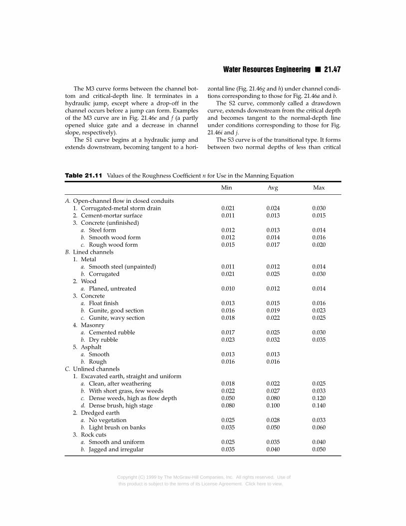
Water Resources Engineering n 21.47
The M3 curve forms between the channel bot-tom and critical-depth line. It terminates in ahydraulic jump, except where a drop-off in thechannel occurs before a jump can form. Examplesof the M3 curve are in Fig. 21.46e and f (a partlyopened sluice gate and a decrease in channelslope, respectively).
The S1 curve begins at a hydraulic jump andextends downstream, becoming tangent to a hori-
A. Open-channel flow in closed conduits1. Corrugated-metal storm drain2. Cement-mortar surface3. Concrete (unfinished)
a. Steel formb. Smooth wood formc. Rough wood form
B. Lined channels1. Metal
a. Smooth steel (unpainted)b. Corrugated
2. Wooda. Planed, untreated
3. Concretea. Float finishb. Gunite, good sectionc. Gunite, wavy section
4. Masonrya. Cemented rubbleb. Dry rubble
5. Asphalta. Smoothb. Rough
C. Unlined channels1. Excavated earth, straight and uniform
a. Clean, after weatheringb. With short grass, few weedsc. Dense weeds, high as flow depthd. Dense brush, high stage
2. Dredged eartha. No vegetationb. Light brush on banks
3. Rock cutsa. Smooth and uniformb. Jagged and irregular
Table 21.11 Values of the Roughness Coefficient n
Copyright (C) 1999 by The McGraw-Hill Cothis product is subject to the terms of its Lic
zontal line (Fig. 21.46g and h) under channel condi-tions corresponding to those for Fig. 21.46a and b.
The S2 curve, commonly called a drawdowncurve, extends downstream from the critical depthand becomes tangent to the normal-depth lineunder conditions corresponding to those for Fig.21.46i and j.
The S3 curve is of the transitional type. It formsbetween two normal depths of less than critical
Min Avg Max
0.021 0.024 0.0300.011 0.013 0.015
0.012 0.013 0.0140.012 0.014 0.0160.015 0.017 0.020
0.011 0.012 0.0140.021 0.025 0.030
0.010 0.012 0.014
0.013 0.015 0.0160.016 0.019 0.0230.018 0.022 0.025
0.017 0.025 0.0300.023 0.032 0.035
0.013 0.0130.016 0.016
0.018 0.022 0.0250.022 0.027 0.0330.050 0.080 0.1200.080 0.100 0.140
0.025 0.028 0.0330.035 0.050 0.060
0.025 0.035 0.0400.035 0.040 0.050
for Use in the Manning Equation
mpanies, Inc. All rights reserved. Use ofense Agreement. Click here to view.

21.48 n Section Twenty-One
depth under conditions corresponding to those forFig. 21.46k and l.
Examples in Fig. 21.46m through r show condi-tions for the formation of C, H, and A profiles.
Fig. 21.46 Typical flow profiles for channels withC.D.L., critical-depth line.
Copyright (C) 1999 by The McGraw-Hill Cothis product is subject to the terms of its L
The curves in Fig. 21.46 approach the normal-depth line asymptotically and terminate abruptlyin a vertical line as they approach the critical depth.The curves that approach the bottom intersect it at
various slopes. N.D.L. indicates normal-depth line;
mpanies, Inc. All rights reserved. Use oficense Agreement. Click here to view.
Water Resources Engineering n 21.49
a definite angle but are imaginary near the bottomsince velocity would have to be infinite to satisfyEq. (21.77) if the depth were zero. The curves areshown dotted near the critical-depth line as areminder that this portion of the curve does notpossess the same degree of accuracy as the rest ofthe curve because of neglect of vertical componentsof velocity in the calculations. These curves eitherstart or end at what is called a point of control.
A point of control is a physical location in aprismatic channel at which the depth of steadyflow may readily be determined. This depth is usu-ally different from the normal depth for the chan-nel because of a grade change, gate, weir, dam, freeoverfall, or other feature at that location that caus-es a backwater curve to form. Calculations for thelength and shape of the surface profile of a back-water curve start at this known depth and locationand proceed either up or downstream, dependingon the type of flow. For subcritical flow conditions,the curve proceeds upstream from the point ofcontrol in a true backwater curve. The surfacecurve that occurs under supercritical flow condi-tions proceeds downstream from the point of con-trol and might better be called a downwater curve.
The point of control is always at the down-stream end of a backwater curve in subcritical flowand at the upstream end for supercritical flow. Thisis explained as follows: A backwater curve may bethought of as being the result of some disruptionof uniform flow that causes a wave of disturbancein the channel. The wave travels at a speed, knownas its celerity, which always equals the criticalvelocity for the channel. If a disturbance waveattempts to move upstream against supercriticalflow (flow moving at a speed greater than critical),it will be swept downstream by the flow and haveno effect on conditions upstream. A disturbancewave is held steady by critical flow and movesupstream in subcritical flow.
When a hydraulic jump occurs on a mild slopeand is followed by a free overfall (Fig. 21.51), back-water curves form both before and after the jump.The point of control for the curve in the supercrit-ical region above the jump will be located at thevena contracta that forms just below the sluicegate. The point of control for the backwater curvein the subcritical region below the jump is at thefree overfall where critical depth occurs. Computa-tions for these backwater curves are carried towardthe jump from their respective points of control
Copyright (C) 1999 by The McGraw-Hill Cothis product is subject to the terms of its Lic
and are extended across the jump to help deter-mine its exact location. But a backwater curve can-not be calculated through a hydraulic jump fromeither direction. The surface profiles involved ter-minate abruptly in a vertical line as they approachthe critical depth, and a hydraulic jump alwaysoccurs across critical depth. See Art. 21.27.5.
(R. H. French, “Open-Channel Hydraulics,”McGraw-Hill, Inc., New York.)
21.26 Backwater-CurveComputations
The solution of a backwater curve involves compu-tation of a gradually varied flow profile. Solutionsavailable include the graphical-integration, direc-tion-integration, and step methods. Explanations ofboth the graphical- and direct-integration methodsare in V. T. Chow, “Open-Channel Hydraulics,”McGraw-Hill Book Company, New York.
Two variations of the step method include thedirect or uniform method and the standardmethod. They are simple and widely used and areavailable in many software packages.
For step-method computations, the channel isdivided into short lengths, or reaches, with rela-tively small variation. In a series of steps startingfrom a point of control, each reach is solved in suc-cession. Step methods have been developed forchannels with uniform or varying cross sections.
Direct step method of backwater computationinvolves solving for an unknown length of channelbetween two known depths. The procedure isapplicable only to uniform prismatic channels withgradually varying area of flow.
For the section of channel in Fig. 21.47, Bernoulli’sequation for the reach between sections 1 and 2 is
(21.91)
where V1 and V2 = mean velocities of flow atsections 1 and 2, ft/s
d1 and d2 = depths of flow at sections 1and 2, ft
g = acceleration due to gravity,32.2 ft/s2
S– = average head loss due tofriction, ft/ft of channel
mpanies, Inc. All rights reserved. Use ofense Agreement. Click here to view.

21.50 n Section Twenty-One
So = slope of channel bottom
L = length of channel betweensections 1 and 2, ft
Note that SoL = ∆z, the change in elevation, ft, ofthe channel bottom between sections 1 and 2, andS–L = hf, the head loss, ft, due to friction in the samereach. (For uniform, prismatic channels, hi, theeddy loss, is negligible and can be ignored.) S–
equals the slope calculated for the average depthin the reach but may be approximated by the aver-age of the values of friction slope S for the depthsat sections 1 and 2.
Solving Eq. (21.91) for L gives
(21.92)
where He1 and He2 are the specific energy heads forsections 1 and 2, respectively, as given by Eq.(21.82). The friction slope S at any point may becomputed by the Manning equation, rearranged asfollows:
Fig. 21.47 Channel with constant disch
Copyright (C) 1999 by The McGraw-Hill Comthis product is subject to the terms of its Lic
(21.93)
where R = hydraulic radius, ft
n = roughness coefficient (Art. 21.24)
Note that the slope S used in the Manningequation is the slope of the energy grade line, notthe channel bottom. Note also that the roughnesscoefficient n is squared in Eq. (21.93), and its valuemust therefore be chosen with special care to avoidan exaggerated error in the computed frictionslope. The smaller the value of n, the longer thebackwater curve profile, and vice versa. Therefore,the smallest n possible for the prevailing condi-tions should be selected for computation of a back-water curve if knowledge of the longest possibleflow profile is required.
The first step in the direct step method involveschoosing a series of depths for the end points ofeach reach. These depths will range from thedepth at the point of control to the ending depthfor the backwater curve. This ending depth is oftenthe normal depth for the channel (Art. 21.22) but
arge and gradually varying cross section.
panies, Inc. All rights reserved. Use ofense Agreement. Click here to view.
Water Resources Engineering n 21.51
may be some intermediate depth, such as for acurve preceding a hydraulic jump. Depths shouldbe chosen so that the velocity change across areach does not exceed 20% of the velocity at thebeginning of the reach. Also the change in depthbetween sections should never exceed 1 ft.
The specific energy head He should be comput-ed for the chosen depth at each of the various sec-tions and the change in specific energy betweensections determined. Next, the friction slope Sshould be computed at each section from Eq.(21.93). The average of two sections gives the fric-tion slope S– between sections. Finally, the differ-ence between S– and slope of channel bottom Soshould be computed and the length of reach deter-mined from Eq. (21.92).
Standard step method allows computation ofbackwater curves in both nonprismatic naturalchannels and nonuniform artificial channels aswell as in uniform channels. This method involvessolving for the depth of flow at various locationsalong a channel with Bernoulli’s energy equationand a known length of reach.
A surface profile is determined in the followingmanner: The channel is examined for changes incross section, grade, or roughness, and the loca-tions of these changes are given station numbers.Stations are also established between these loca-tions such that the velocity change between anytwo consecutive stations is not greater than 20% ofthe velocity at the former station. Data concerningthe hydraulic elements of the channel are collectedat each station. Computation of the surface curve isthen made in steps, starting from the point of con-trol and progressing from station to station—in anupstream direction for subcritical flow and down-stream for supercritical flow. The length of reach ineach step is given by the stationing, and the depthof flow is determined by trial and error.
Nonprismatic channels do not have well-defined points of control to aid in determining thestarting depth for a backwater curve. Therefore,the water-surface elevation at the beginning mustbe determined as follows:
The step computations are started at a point inthe channel some distance upstream or downstreamfrom the desired starting point, depending onwhether flow is supercritical or subcritical, respec-tively. Then, computations progress toward the ini-tial section. Since this step method is a convergingprocess, this procedure produces the true depth for
Copyright (C) 1999 by The McGraw-Hill Cothis product is subject to the terms of its Lic
the initial section within a relatively few steps. The energy balance used in the standard step
method is shown graphically in Fig. 21.47, in whichthe position of the water surface at section 1 is Z1and at section 2, Z2, referred to a horizontal datum.Writing Bernoulli’s equation [Eq. (21.11)] for sec-tions 1 and 2 Yields
(21.94)
where V1 and V2 are the mean velocities, ft/s, at sec-tions 1 and 2; the friction loss, ft, in the reach (S–L )is denoted by hf; and the term hi is added toaccount for eddy loss, ft.
Eddy loss, sometimes called impact loss, is ahead loss caused by flow running contrary to themain current because of irregularities in the chan-nel. No rational method is available for determina-tion of eddy loss, and it is therefore often accountedfor, in natural channels, by a slight increase in Man-ning’s n. Eddy loss depends mainly on a change invelocity head. For lined channels, it has beenexpressed as a coefficient k to be applied as follows:
(21.95)
The coefficient k is 0.2 for diverging reaches, from0 to 0.1 for converging reaches, and about 0.5 forabrupt expansions and contractions.
The total head at any section of the channel is
(21.96)
where Z equals the elevation of the channel bot-tom above the given datum plus the depth of flowd at that section. Friction slope S is computed fromEq. (21.93). Then, S–, the average friction slope forthe reach, is calculated as the mean of the slope forthe section and the preceding section. Friction losshf is the product of S–and the length of the reach L.Eddy loss hi is found from Eq. (21.95). Next, totalhead H, ft, is obtained from Eq. (21.94), which, aftersubstitution of H from Eq. (21.96), becomes
(21.97)
where H1 and H2 equal the total head of sections 1and 2, respectively. The value of total head com-puted from Eq. (21.97) must agree with the value of
mpanies, Inc. All rights reserved. Use ofense Agreement. Click here to view.
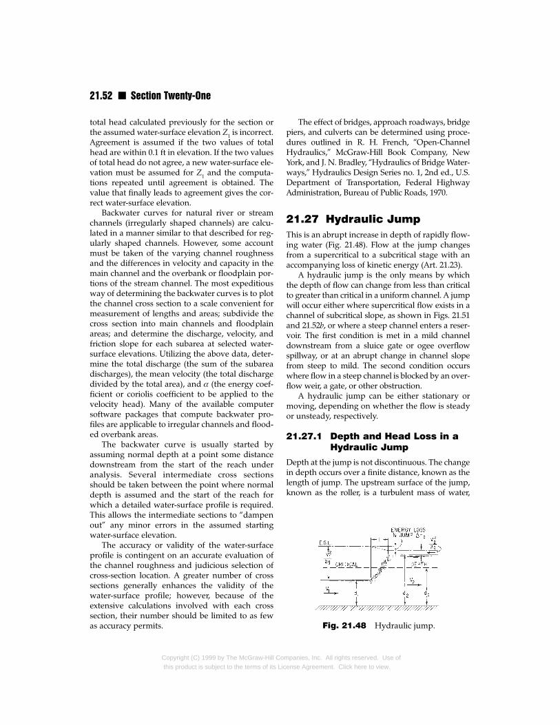
21.52 n Section Twenty-One
total head calculated previously for the section orthe assumed water-surface elevation Z1 is incorrect.Agreement is assumed if the two values of totalhead are within 0.1 ft in elevation. If the two valuesof total head do not agree, a new water-surface ele-vation must be assumed for Z1 and the computa-tions repeated until agreement is obtained. Thevalue that finally leads to agreement gives the cor-rect water-surface elevation.
Backwater curves for natural river or streamchannels (irregularly shaped channels) are calcu-lated in a manner similar to that described for reg-ularly shaped channels. However, some accountmust be taken of the varying channel roughnessand the differences in velocity and capacity in themain channel and the overbank or floodplain por-tions of the stream channel. The most expeditiousway of determining the backwater curves is to plotthe channel cross section to a scale convenient formeasurement of lengths and areas; subdivide thecross section into main channels and floodplainareas; and determine the discharge, velocity, andfriction slope for each subarea at selected water-surface elevations. Utilizing the above data, deter-mine the total discharge (the sum of the subareadischarges), the mean velocity (the total dischargedivided by the total area), and α (the energy coef-ficient or coriolis coefficient to be applied to thevelocity head). Many of the available computersoftware packages that compute backwater pro-files are applicable to irregular channels and flood-ed overbank areas.
The backwater curve is usually started byassuming normal depth at a point some distancedownstream from the start of the reach underanalysis. Several intermediate cross sectionsshould be taken between the point where normaldepth is assumed and the start of the reach forwhich a detailed water-surface profile is required.This allows the intermediate sections to “dampenout” any minor errors in the assumed startingwater-surface elevation.
The accuracy or validity of the water-surfaceprofile is contingent on an accurate evaluation ofthe channel roughness and judicious selection ofcross-section location. A greater number of crosssections generally enhances the validity of thewater-surface profile; however, because of theextensive calculations involved with each crosssection, their number should be limited to as fewas accuracy permits.
Copyright (C) 1999 by The McGraw-Hill Comthis product is subject to the terms of its Lic
The effect of bridges, approach roadways, bridgepiers, and culverts can be determined using proce-dures outlined in R. H. French, “Open-ChannelHydraulics,” McGraw-Hill Book Company, NewYork, and J. N. Bradley, “Hydraulics of Bridge Water-ways,” Hydraulics Design Series no. 1, 2nd ed., U.S.Department of Transportation, Federal HighwayAdministration, Bureau of Public Roads, 1970.
21.27 Hydraulic JumpThis is an abrupt increase in depth of rapidly flow-ing water (Fig. 21.48). Flow at the jump changesfrom a supercritical to a subcritical stage with anaccompanying loss of kinetic energy (Art. 21.23).
A hydraulic jump is the only means by whichthe depth of flow can change from less than criticalto greater than critical in a uniform channel. A jumpwill occur either where supercritical flow exists in achannel of subcritical slope, as shown in Figs. 21.51and 21.52b, or where a steep channel enters a reser-voir. The first condition is met in a mild channeldownstream from a sluice gate or ogee overflowspillway, or at an abrupt change in channel slopefrom steep to mild. The second condition occurswhere flow in a steep channel is blocked by an over-flow weir, a gate, or other obstruction.
A hydraulic jump can be either stationary ormoving, depending on whether the flow is steadyor unsteady, respectively.
21.27.1 Depth and Head Loss in aHydraulic Jump
Depth at the jump is not discontinuous. The changein depth occurs over a finite distance, known as thelength of jump. The upstream surface of the jump,known as the roller, is a turbulent mass of water,
Fig. 21.48 Hydraulic jump.
panies, Inc. All rights reserved. Use ofense Agreement. Click here to view.

Water Resources Engineering n 21.53
which is continually tumbling erratically against therapidly flowing sheet below.
The depth before a jump is the initial depth,and the depth after a jump is the sequent depth.The specific energy for the sequent depth is lessthan that for the initial depth because of the ener-gy dissipation within the jump. (Initial andsequent depths should not be confused with thedepths of equal energy, or alternate depths.)
According to Newton’s second law of motion,the rate of loss of momentum at the jump mustequal the unbalanced pressure force acting on themoving water and tending to retard its motion.This unbalanced force equals the differencebetween the hydrostatic forces corresponding tothe depths before and after the jump. For rectan-gular channels, this resultant pressure force is
(21.98)
where d1 = depth before jump, ft
d2 = depth after jump, ft
w = unit weight of water, lb/ft3
The rate of change of momentum at the jump perfoot width of channel equals
(21.99)
where M = mass of water, lb⋅s2/ft
V1 = velocity at depth d1, ft/s
V2 = velocity at depth d2, ft/s
q = discharge per foot width of rectan-gular channel, ft3/s
t = unit of time, s
g = acceleration due to gravity, 32.2 ft/s2
Equating the values of F in Eqs. (21.98) and (21.99),and substituting V1d1 for q and V1d1/d2 for V2, thereduced equation for rectangular channels becomes
(21.100)
Equation (21.100) may then be solved for thesequent depth:
(21.101)
Copyright (C) 1999 by The McGraw-Hill Cothis product is subject to the terms of its Lic
If V2d2/d1 is substituted for V1, in Eq. (21.100),
(21.102)
Equation (21.102) may be used in determining theposition of the jump where V2 and d2 are known.Relationships may be derived similarly for chan-nels of any cross section.
The head loss in a jump equals the difference inspecific-energy head before and after the jump.This difference (Fig. 21.49) is given by
(21.103)
where He1 = specific-energy head of stream beforejump, ft
He2 = specific-energy head of stream afterjump, ft
The specific energy for free-surface flow is givenby Eq. (21.82).
The depths before and after a hydraulic jumpmay be related to the critical depth by the equation
(21.104)
where q = discharge, ft3/s per ft of channelwidth
dc = critical depth for the channel, ft
It may be seen from this equation that if d1 = dc, d2must also equal dc.
21.27.2 Jump in HorizontalRectangular Channels
The form of a hydraulic jump in a horizontal rec-tangular channel may be of several distinct types,depending on the Froude number of the incomingflow F = V/(gL)1/2 [Eq. (21.16)], where L is a charac-teristic length, ft; V is the mean velocity, ft/s; and g= acceleration due to gravity, ft/s2. For open-chan-nel flow, the characteristic length for the Froudenumber is made equal to the hydraulic depth dh.
Hydraulic depth is defined as
(21.105)
where A = area of flow, ft2
T = width of free surface, ft
mpanies, Inc. All rights reserved. Use ofense Agreement. Click here to view.

21.54 n Section Twenty-One
For rectangular channels, hydraulic depth equalsdepth of flow.
Various forms of hydraulic jump, and their rela-tion to the Froude number of the approaching flowF1, were classified by the U.S. Bureau of Reclama-tion and are presented in Fig. 21.49.
For F1 = 1, the flow is critical and there is nojump.
For F1 = 1 to 1.7, there are undulations on thesurface. The jump is called an undular jump.
For F1 = 1.7 to 2.5, a series of small rollers devel-op on the surface of the jump, but the downstreamwater surface remains smooth. The velocitythroughout is fairly uniform and the energy loss islow. This jump may be called a weak jump.
For F1 = 2.5 to 4.5, an oscillating jet is enteringthe jump. The jet moves from the channel bottomto the surface and back again with no set period.Each oscillation produces a large wave of irregularperiod, which, very commonly in canals, can trav-
Fig. 21.49 Type of hydraulic jump depends onFroude number.
Copyright (C) 1999 by The McGraw-Hill Comthis product is subject to the terms of its Lic
el for miles, doing extensive damage to earth banksand riprap surfaces. This jump may be called anoscillating jump.
For F1 = 4.5 to 9.0, the downstream extremity ofthe surface roller and the point at which the high-velocity jet tends to leave the flow occur at practi-cally the same vertical section. The action and posi-tion of this jump are least sensitive to variation intailwater depth. The jump is well-balanced, andthe performance is at its best. The energy dissipa-tion ranges from 45 to 70%. This jump may becalled a steady jump.
For F1 = 9.0 and larger, the high-velocity jet grabsintermittent slugs of water rolling down the frontface of the jump, generating waves downstream andcausing a rough surface. The jump action is roughbut effective, and energy dissipation may reach 85%.This jump may be called a strong jump.
Note that the ranges of the Froude numbergiven for the various types of jump are not clear-cut but overlap to a certain extent, depending onlocal conditions.
21.27.3 Hydraulic Jump as anEnergy Dissipator
A hydraulic jump is a useful means for dissipatingexcess energy in supercritical flow (Art. 21.23). Ajump may be used to prevent erosion below anoverflow spillway, chute, or sluice gate by quicklyreducing the velocity of the flow over a pavedapron. A special section of channel built to containa hydraulic jump is known as a stilling basin.
If a hydraulic jump is to function ideally as anenergy dissipator, below a spillway, for example,the elevation of the water surface after the jumpmust coincide with the normal tailwater elevationfor every discharge. If the tailwater is too low, thehigh-velocity flow will continue downstream forsome distance before the jump can occur. If the tail-water is too high, the jump will be drowned out,and there will be a much smaller dissipation of totalhead. In either case, dangerous erosion is likely tooccur for a considerable distance downstream.
The ideal condition is to have the sequent-depthcurve, which gives discharge vs. depth after thejump, coincide exactly with the tailwater-ratingcurve. The tailwater-rating curve gives normaldepths in the discharge channel for the range offlows to be expected. Changes in the spillwaydesign that can be made to alter the tailwater-rating
panies, Inc. All rights reserved. Use ofense Agreement. Click here to view.

Water Resources Engineering n 21.55
curve involve changing the crest length, changingthe apron elevation, and sloping the apron.
Accessories, such as chute blocks and baffleblocks are usually installed in a stilling basin tocontrol the jump. The main purpose of these acces-sories is to shorten the range within which thejump will take place, not only to force the jump tooccur within the basin but to reduce the size andtherefore the cost of the basin. Controls within astilling basin have additional advantages in thatthey improve the dissipation function of the basinand stabilize the jump action.
21.27.4 Length of Hydraulic Jump
The length of a hydraulic jump L may be defined asthe horizontal distance from the upstream edge ofthe roller to a point on the raised surface immedi-ately downstream from cessation of the violent tur-bulence. This length (Fig. 21.48) defies accuratemathematical expression, partly because of thenonuniform velocity distribution within the jump.But it has been determined experimentally. Theexperimental results may be summarized conve-niently by plotting the Froude number of theupstream flow F1 against a dimensionless ratio ofjump length to downstream depth L/d2. The result-ing curve (Fig. 21.50) has a flat portion in the rangeof steady jumps. The curve thus minimizes theeffect of any errors made in calculation of the
Fig. 21.50 Length of hydraulic jump in a horizonFroude number of the approaching flow.
Copyright (C) 1999 by The McGraw-Hill Cothis product is subject to the terms of its Lic
Froude number in the range where this informationis most frequently needed. The curve, prepared byV. T. Chow from data gathered by the U.S. Bureau ofReclamation, was developed for jumps in rectangu-lar channels, but it will give approximate results forjumps formed in trapezoidal channels.
For other than rectangular channels the depthd1 used in the equation for Froude number is thehydraulic depth given by Eq. (21.105).
21.27.5 Location of a HydraulicJump
It is important to know where a hydraulic jumpwill form since the turbulent energy released in ajump can extensively scour an unlined channel ordestroy paving in a thinly lined channel. Specialreinforced sections of channel must be built towithstand the pounding and vibration of a jumpand to provide extra freeboard for the added depthat the jump. These features are expensive to build;therefore, a great savings can be realized if theiruse is restricted to a limited area through a knowl-edge of the jump location.
The precision with which the location is pre-dicted depends on the accuracy with which thefriction losses and length of jump are estimatedand on whether the discharge is as assumed. Themethod of prediction used for rectangular chan-nels is illustrated for a sluice gate in Fig. 21.51.
tal channel depends on sequent depth d2 and the
mpanies, Inc. All rights reserved. Use ofense Agreement. Click here to view.
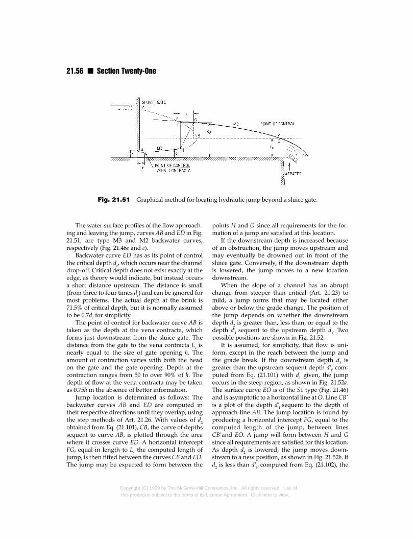
21.56 n Section Twenty-One
Fig. 21.51 Graphical method for locating hydraulic jump beyond a sluice gate.
The water-surface profiles of the flow approach-ing and leaving the jump, curves AB and ED in Fig.21.51, are type M3 and M2 backwater curves,respectively (Fig. 21.46e and c).
Backwater curve ED has as its point of controlthe critical depth dc, which occurs near the channeldrop-off. Critical depth does not exist exactly at theedge, as theory would indicate, but instead occursa short distance upstream. The distance is small(from three to four times dc) and can be ignored formost problems. The actual depth at the brink is71.5% of critical depth, but it is normally assumedto be 0.7dc for simplicity.
The point of control for backwater curve AB istaken as the depth at the vena contracta, whichforms just downstream from the sluice gate. Thedistance from the gate to the vena contracta Le isnearly equal to the size of gate opening h. Theamount of contraction varies with both the headon the gate and the gate opening. Depth at thecontraction ranges from 50 to over 90% of h. Thedepth of flow at the vena contracta may be takenas 0.75h in the absence of better information.
Jump location is determined as follows: Thebackwater curves AB and ED are computed intheir respective directions until they overlap, usingthe step methods of Art. 21.26. With values of d2obtained from Eq. (21.101), CB, the curve of depthssequent to curve AB, is plotted through the areawhere it crosses curve ED. A horizontal interceptFG, equal in length to L, the computed length ofjump, is then fitted between the curves CB and ED.The jump may be expected to form between the
Copyright (C) 1999 by The McGraw-Hill Comthis product is subject to the terms of its Lic
points H and G since all requirements for the for-mation of a jump are satisfied at this location.
If the downstream depth is increased becauseof an obstruction, the jump moves upstream andmay eventually be drowned out in front of thesluice gate. Conversely, if the downstream depthis lowered, the jump moves to a new locationdownstream.
When the slope of a channel has an abruptchange from steeper than critical (Art. 21.23) tomild, a jump forms that may be located eitherabove or below the grade change. The position ofthe jump depends on whether the downstreamdepth d2 is greater than, less than, or equal to thedepth d′1 sequent to the upstream depth d1. Twopossible positions are shown in Fig. 21.52.
It is assumed, for simplicity, that flow is uni-form, except in the reach between the jump andthe grade break. If the downstream depth d2 isgreater than the upstream sequent depth d′1, com-puted from Eq. (21.101) with d1 given, the jumpoccurs in the steep region, as shown in Fig. 21.52a.The surface curve EO is of the S1 type (Fig. 21.46)and is asymptotic to a horizontal line at O. Line CB′is a plot of the depth d′1 sequent to the depth ofapproach line AB. The jump location is found byproducing a horizontal intercept FG, equal to thecomputed length of the jump, between linesCB′and EO. A jump will form between H and Gsince all requirements are satisfied for this location.As depth d2 is lowered, the jump moves down-stream to a new position, as shown in Fig. 21.52b. Ifd2 is less than d′1 , computed from Eq. (21.102), the
panies, Inc. All rights reserved. Use ofense Agreement. Click here to view.
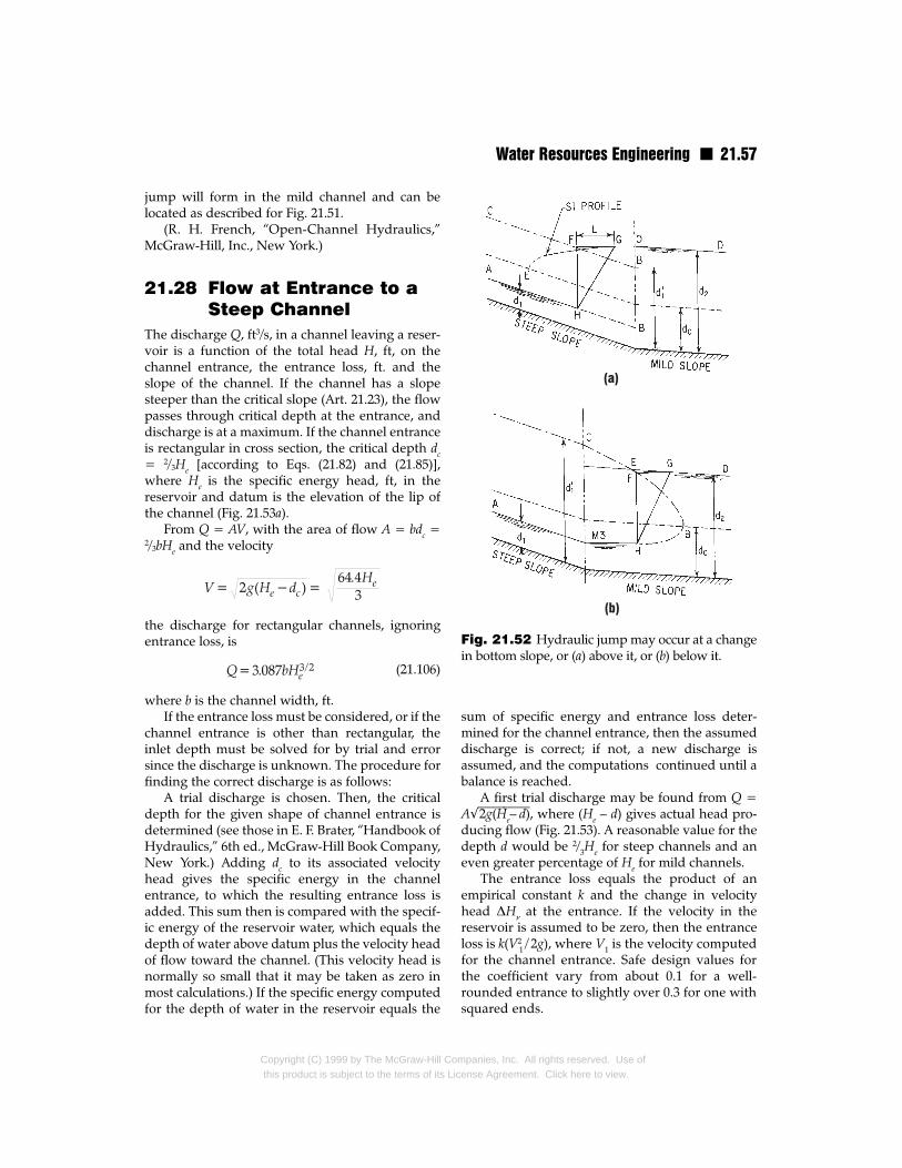
Water Resources Engineering n 21.57
jump will form in the mild channel and can belocated as described for Fig. 21.51.
(R. H. French, “Open-Channel Hydraulics,”McGraw-Hill, Inc., New York.)
21.28 Flow at Entrance to aSteep Channel
The discharge Q, ft3/s, in a channel leaving a reser-voir is a function of the total head H, ft, on thechannel entrance, the entrance loss, ft. and theslope of the channel. If the channel has a slopesteeper than the critical slope (Art. 21.23), the flowpasses through critical depth at the entrance, anddischarge is at a maximum. If the channel entranceis rectangular in cross section, the critical depth dc= 2/3He [according to Eqs. (21.82) and (21.85)],where He is the specific energy head, ft, in thereservoir and datum is the elevation of the lip ofthe channel (Fig. 21.53a).
From Q = AV, with the area of flow A = bdc =2/3bHe and the velocity
the discharge for rectangular channels, ignoringentrance loss, is
(21.106)
where b is the channel width, ft. If the entrance loss must be considered, or if the
channel entrance is other than rectangular, theinlet depth must be solved for by trial and errorsince the discharge is unknown. The procedure forfinding the correct discharge is as follows:
A trial discharge is chosen. Then, the criticaldepth for the given shape of channel entrance isdetermined (see those in E. F. Brater, “Handbook ofHydraulics,” 6th ed., McGraw-Hill Book Company,New York.) Adding dc to its associated velocityhead gives the specific energy in the channelentrance, to which the resulting entrance loss isadded. This sum then is compared with the specif-ic energy of the reservoir water, which equals thedepth of water above datum plus the velocity headof flow toward the channel. (This velocity head isnormally so small that it may be taken as zero inmost calculations.) If the specific energy computedfor the depth of water in the reservoir equals the
Copyright (C) 1999 by The McGraw-Hill Cothis product is subject to the terms of its Lic
sum of specific energy and entrance loss deter-mined for the channel entrance, then the assumeddischarge is correct; if not, a new discharge isassumed, and the computations continued until abalance is reached.
A first trial discharge may be found from Q =A√
——2g(He– d)——, where (He – d) gives actual head pro-ducing flow (Fig. 21.53). A reasonable value for thedepth d would be 2/3He for steep channels and aneven greater percentage of He for mild channels.
The entrance loss equals the product of anempirical constant k and the change in velocityhead ∆Hν at the entrance. If the velocity in thereservoir is assumed to be zero, then the entranceloss is k(V2
1 / 2g), where V1 is the velocity computedfor the channel entrance. Safe design values forthe coefficient vary from about 0.1 for a well-rounded entrance to slightly over 0.3 for one withsquared ends.
Fig. 21.52 Hydraulic jump may occur at a changein bottom slope, or (a) above it, or (b) below it.
mpanies, Inc. All rights reserved. Use ofense Agreement. Click here to view.

21.58 n Section Twenty-One
Fig. 21.53 Flow at entrance to (a) steep channel; (b) mild-slope channel.
21.29 Flow at Entrance to aChannel of Mild Slope
When water flows from a reservoir into a channelwith slope less than the critical slope (Art. 21.23),the depth of flow at the channel entrance equalsthe normal depth for the channel (Art. 21.22). Theentrance depth and discharge are dependent oneach other. The discharge that results from a givenhead is that for which flow enters the channelwithout forming either a backwater or drawdowncurve within the entrance. This requirement neces-sitates the formation of normal depth d since onlyat this equilibrium depth is there no tendency tochange the discharge or to form backwater curves.(In Fig. 21.53b, d is normal depth.)
A solution for discharge at entrance to a chan-nel of mild slope is found as follows: A trial dis-
Copyright (C) 1999 by The McGraw-Hill Cothis product is subject to the terms of its Li
charge, ft3/s, is estimated from Q = A√——2g(He– d)——,
where He – d is the actual head, ft, producing flow.He is the specific energy head, ft, of the reservoirwater relative to datum at lip of channel; A is thecross-sectional area of flow, ft2; and g is accelerationdue to gravity, 32.2 ft/s2. The normal depth of thechannel is determined for this discharge from Eq.(21.83). The velocity head is computed for thisdepth-discharge combination, and an entrance-losscalculation is made (see Art. 21.33). The sum of thespecific energy of flow in the channel entrance andthe entrance loss must equal the specific energy ofthe water in the reservoir for an energy balance toexist between those points (Fig. 21.53b). If the trialdischarge gives this balance of energy, then the dis-charge is correct; if not, a new discharge is chosen,and the calculations continued until a satisfactorybalance is obtained.
mpanies, Inc. All rights reserved. Use ofcense Agreement. Click here to view.

Water Resources Engineering n 21.59
21.30 Channel Section ofGreatest Efficiency
If a channel of any shape is to reach its greatesthydraulic efficiency, it must have the shortest possi-ble wetted perimeter for a given cross-sectional area.The resulting shape gives the greatest hydraulicradius and therefore the greatest capacity for thatarea. This can be seen from the Manning equationfor discharge [Eq. (21.83)], in which Q is a directfunction of hydraulic radius to the two-thirds power.
The most efficient of all possible open-channelcross sections is the semicircle. There are practicalobjections to the use of this shape because of thedifficulty of construction, but it finds some use inmetal flumes where sections can be preformed.The most efficient of all trapezoidal sections is thehalf hexagon, which is used extensively for largewater-supply channels. The rectangular sectionwith the greatest efficiency has a depth of flowequal to one-half the width. This shape is oftenused for box culverts and small drainage ditches.
21.31 Subcritical Flow aroundBends in Channels
Because of the inability of liquids to resist shearingstress, the free surface of steady uniform flow isalways normal to the resultant of the forces actingon the water. Water in a reservoir has a horizontalsurface since the only force acting on it is the forceof gravity.
Water reacts in accordance with Newton’s firstlaw of motion: It flows in a straight line unlessdeflected from its path by an outside force. Whenwater is forced to flow in a curved path, its surfaceassumes a position normal to the resultant of theforces of gravity and radial acceleration. The forcedue to radial acceleration equals the force requiredto turn the water from a straight-line path, ormV2 /rc for m, a unit mass of water, where V is itsaverage velocity, ft /s, and rc the radius of curva-ture, ft, of the center line of the channel.
The water surface makes an angle φ with thehorizontal such that
(21.107)
The theoretical difference y, ft. in water-surfacelevel between the inside and outside banks of a
Copyright (C) 1999 by The McGraw-Hill Cothis product is subject to the terms of its Lic
curve (Fig. 21.54) is found by multiplying tan φ bythe top width of the channel T, ft. Thus,
(21.108)
where the radius of curvature rc of the center of thechannel is assumed to represent the average cur-vature of flow. This equation gives values of ysmaller than those actually encountered because ofthe use of average values of velocity and radius,rather than empirically derived values more repre-sentative of actual conditions. The error will not begreat, however, if the depth of flow is well abovecritical (Art. 21.23). In this range, the true value ofy would be only a few inches.
The difference in surface elevation found fromEq. (21.108), although it involves some drop in sur-face elevation on the inside of the curve, does notallow a savings of freeboard height on the insidebank. The water surface there is wavy and thusneeds a freeboard height at least equal to that of astraight channel.
The top layer of flow in a channel has a highervelocity than flow near the bottom because of theretarding effect of friction along the floor of the chan-nel. A greater force is required to deflect the high-velocity flow. Therefore, when a stream enters acurve, the higher-velocity flow moves to the outsideof the bend. If the bend continues long enough, allthe high-velocity water will move against the outerbank and may cause extensive scour unless specialbank protection is provided.
Fig. 21.54 Water-surface profile at a bend in achannel with subcritical flow.
mpanies, Inc. All rights reserved. Use ofense Agreement. Click here to view.
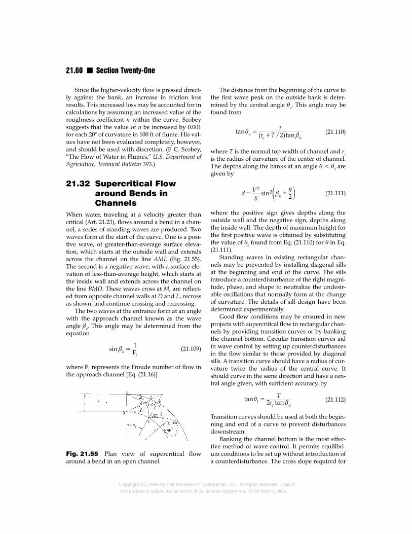
21.60 n Section Twenty-One
Since the higher-velocity flow is pressed direct-ly against the bank, an increase in friction lossresults. This increased loss may be accounted for incalculations by assuming an increased value of theroughness coefficient n within the curve. Scobeysuggests that the value of n be increased by 0.001for each 20° of curvature in 100 ft of flume. His val-ues have not been evaluated completely, however,and should be used with discretion. (F. C. Scobey,“The Flow of Water in Flumes,” U.S. Department ofAgriculture, Technical Bulletin 393.)
21.32 Supercritical Flowaround Bends inChannels
When water, traveling at a velocity greater thancritical (Art. 21.23), flows around a bend in a chan-nel, a series of standing waves are produced. Twowaves form at the start of the curve. One is a posi-tive wave, of greater-than-average surface eleva-tion, which starts at the outside wall and extendsacross the channel on the line AME (Fig. 21.55).The second is a negative wave, with a surface ele-vation of less-than-average height, which starts atthe inside wall and extends across the channel onthe line BMD. These waves cross at M, are reflect-ed from opposite channel walls at D and E, recrossas shown, and continue crossing and recrossing.
The two waves at the entrance form at an anglewith the approach channel known as the waveangle βo. This angle may be determined from theequation
(21.109)
where F1 represents the Froude number of flow inthe approach channel [Eq. (21.16)] .
Fig. 21.55 Plan view of supercritical flowaround a bend in an open channel.
Copyright (C) 1999 by The McGraw-Hill Comthis product is subject to the terms of its Lic
The distance from the beginning of the curve tothe first wave peak on the outside bank is deter-mined by the central angle θo. This angle may befound from
(21.110)
where T is the normal top width of channel and rcis the radius of curvature of the center of channel.The depths along the banks at an angle θ < θo aregiven by
(21.111)
where the positive sign gives depths along theoutside wall and the negative sign, depths alongthe inside wall. The depth of maximum height forthe first positive wave is obtained by substitutingthe value of θo found from Eq. (21.110) for θ in Eq.(21.111).
Standing waves in existing rectangular chan-nels may be prevented by installing diagonal sillsat the beginning and end of the curve. The sillsintroduce a counterdisturbance of the right magni-tude, phase, and shape to neutralize the undesir-able oscillations that normally form at the changeof curvature. The details of sill design have beendetermined experimentally.
Good flow conditions may be ensured in newprojects with supercritical flow in rectangular chan-nels by providing transition curves or by bankingthe channel bottom. Circular transition curves aidin wave control by setting up counterdisturbancesin the flow similar to those provided by diagonalsills. A transition curve should have a radius of cur-vature twice the radius of the central curve. Itshould curve in the same direction and have a cen-tral angle given, with sufficient accuracy, by
(21.112)
Transition curves should be used at both the begin-ning and end of a curve to prevent disturbancesdownstream.
Banking the channel bottom is the most effec-tive method of wave control. It permits equilibri-um conditions to be set up without introduction ofa counterdisturbance. The cross slope required for
panies, Inc. All rights reserved. Use ofense Agreement. Click here to view.

Water Resources Engineering n 21.61
equilibrium is the same as the surface slope foundfor subcritical flow around a bend (Fig. 21.54). Theangle φ the bottom makes with the horizontal isfound from the equation
(21.113)
21.33 Transitions in OpenChannels
A transition is a structure placed between twoopen channels of different shape or cross-sectionalarea to produce a smooth, low-head-loss transferof flow. The major problems associated withdesign of a transition lie in locating the invert anddetermining the various cross-sectional areas sothat the flow is in accord with the assumptionsmade in locating the invert. Many variables, suchas flow-rate changes, wall roughness, and channelshape and slope, must be taken into account indesign of a smooth-flow transition.
When proceeding downstream through a tran-sition, the flow may remain subcritical or super-critical (Art. 21.23), change from subcritical tosupercritical, or change from supercritical to sub-critical. The latter flow possibility may produce ahydraulic jump.
Special care must be exercised in the design ifthe depth in either of the two channels connectedis near the critical depth. In this range, a smallchange in energy head within the transition maycause the depth of flow to change to its alternatedepth. A flow that switches to its subcritical alter-nate depth may overflow the channel. A flow thatchanges to its supercritical alternate depth maycause excessive channel scour. The relationship offlow depth to energy head can be shown on a plotsuch as Fig. 21.44, p. 21.44.
To place a transition properly between twoopen channels, it is necessary to determine thedesign flow and calculate normal and criticaldepths for each channel section. Maximum flow isusually selected as the design flow. Normal depthfor each section is used for the design depth. Afterthe design has been completed for maximum flow,hydraulic calculations should be made to check thesuitability of the structure for lower flows.
The transition length that produces a smooth-flowing, low-head-loss structure is obtained for an
Copyright (C) 1999 by The McGraw-Hill Comthis product is subject to the terms of its Lic
angle of about 12.5° between the channel axis andthe lines of intersection of the water surface withthe channel sides, as shown in Fig. 21.56. Thelength of the transition Lt is then given by
(21.114)
where T2 and T1 are the top widths of sections 2and 1, respectively.
In design of an inlet-type transition structure,the water-surface level of the downstream channelmust be set below the water-surface level of theupstream channel by at least the sum of theincrease in velocity head, plus any transition andfriction losses. The transition loss, ft, is given byK(∆V2/2g), where K, the loss factor, equals about 0.1for an inlet-type structure; ∆V is the velocitychange, ft/s; and g = 32.2 ft/s2. The total drop inwater surface yd across the inlet-type transition isthen 1.1 [∆(V2/2g)], if friction is ignored.
For outlet-type structures, the average velocitydecreases, and part of the loss in velocity head isrecovered as added depth. The rise of the watersurface for an outlet structure equals the decreasein velocity head minus the outlet and friction loss-es. The outlet loss factor is normally 0.2 for well-designed transitions. If friction is ignored, the totalrise in water surface yr across the outlet structure is0.8[∆(V2/2g)].
Many well-designed transitions have a reverseparabolic water-surface curve tangent to the watersurfaces in each channel (Fig. 21.57). After such awater-surface profile is chosen, depth and cross-sectional areas are selected at points along thetransition to produce this smooth curve. Straight,angular walls usually will not produce a smoothparabolic water surface; therefore, a transitionwith a curved bottom or sides has to be designed.
Fig. 21.56 Plan view of a transition betweentwo open channels with different widths.
panies, Inc. All rights reserved. Use ofense Agreement. Click here to view.
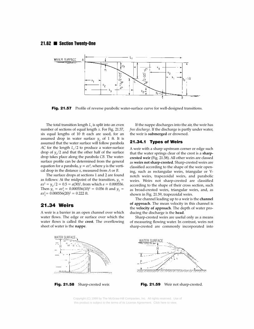
21.62 n Section Twenty-One
Fig. 21.57 Profile of reverse parabolic water-surface curve for well-designed transitions.
The total transition length Lt is split into an evennumber of sections of equal length x. For Fig. 21.57,six equal lengths of 10 ft each are used, for anassumed drop in water surface yd of 1 ft. It isassumed that the water surface will follow parabolaAC for the length Lt / 2 to produce a water-surfacedrop of yd /2 and that the other half of the surfacedrop takes place along the parabola CB. The water-surface profile can be determined from the generalequation for a parabola, y = ax2, where y is the verti-cal drop in the distance x, measured from A or B.
The surface drops at sections 1 and 2 are foundas follows: At the midpoint of the transition, y3 =ax2 = yd / 2 = 0.5 = a(30)2, from which a = 0.000556.Then y1 = ax2
1 = 0.000556(10)2 = 0.056 ft and y2 =ax2
2= 0.000556(20)2 = 0.222 ft.
21.34 WeirsA weir is a barrier in an open channel over whichwater flows. The edge or surface over which thewater flows is called the crest. The overflowingsheet of water is the nappe.
Fig. 21.58 Sharp-crested weir.
Copyright (C) 1999 by The McGraw-Hill Cothis product is subject to the terms of its Lic
If the nappe discharges into the air, the weir hasfree discharge. If the discharge is partly under water,the weir is submerged or drowned.
21.34.1 Types of Weirs
A weir with a sharp upstream corner or edge suchthat the water springs clear of the crest is a sharp-
crested weir (Fig. 21.58). All other weirs are classedas weirs not sharp-crested. Sharp-crested weirs areclassified according to the shape of the weir open-ing, such as rectangular weirs, triangular or V-notch weirs, trapezoidal weirs, and parabolicweirs. Weirs not sharp-crested are classifiedaccording to the shape of their cross section, suchas broad-crested weirs, triangular weirs, and, asshown in Fig. 21.59, trapezoidal weirs.
The channel leading up to a weir is the channel
of approach. The mean velocity in this channel isthe velocity of approach. The depth of water pro-ducing the discharge is the head.
Sharp-crested weirs are useful only as a meansof measuring flowing water. In contrast, weirs notsharp-crested are commonly incorporated into
Fig. 21.59 Weir not sharp-crested.
mpanies, Inc. All rights reserved. Use ofense Agreement. Click here to view.

Water Resources Engineering n 21.63
hydraulic structures as control or regulationdevices, with measurement of flow as their sec-ondary function.
21.34.2 Rectangular Sharp-CrestedWeirs
Discharge over a rectangular sharp-crested weir isgiven by
(21.115)
where Q = discharge, ft3/s
C = discharge coefficient
L = effective length of crest, ft
H = measured head = depth of flowabove elevation of crest, ft
The head should be measured at least 2.5H upstreamfrom the weir, to be beyond the drop in the watersurface (surface contraction) near the weir.
Numerous equations have been developed forfinding the discharge coefficient C. One such equa-tion, which applies only when the nappe is fullyventilated, was developed by Rehbock and simpli-fied by Chow:
(21.116)
where P is the height of the weir above the chan-nel bottom (Fig. 21.58) (V. T. Chow, “Open-Chan-nel Hydraulics,” McGraw-Hill Book Company,New York).
The height of weir P must be at least 2.5H for acomplete crest contraction to form. If P is less than
Fig. 21.60
Copyright (C) 1999 by The McGraw-Hill Cothis product is subject to the terms of its L
2.5H, the crest contraction is reduced and said to bepartly suppressed. Equation (21.116) corrects forthe effects of friction, contraction of the nappe,unequal velocities in the channel of approach, andpartial suppression of the crest contraction andincludes a correction for the velocity of approachand the associated velocity head.
To be fully ventilated, a nappe must have itslower surface subjected to full atmospheric pres-sure. A partial vacuum below the nappe can resultthrough removal of air by the overflowing jet ifthere is restricted ventilation at the sides of theweir. This lack of ventilation causes increased dis-charge and a fluctuation and shape change of thenappe. The resulting unsteady condition is veryobjectionable when the weir is used as a measur-ing device.
At very low heads, the nappe has a tendency toadhere to the downstream face of a rectangularweir even when means for ventilation are provid-ed. A weir operating under such conditions couldnot be expected to have the same relationshipbetween head and discharge as would a fully ven-tilated nappe.
A V-notch weir (Fig. 21.60) should be used formeasurement of flow at very low heads if accuracyof measurement is required.
End contractions occur when the weir open-ing does not extend the full width of theapproach channel. Water flowing near the wallsmust move toward the center of the channel topass over the weir, thus causing a contraction ofthe flow. The nappe continues to contract as itpasses over the crest. Hence, below the crest, thenappe has a minimum width less than the crestlength.
V-notch weir.
mpanies, Inc. All rights reserved. Use oficense Agreement. Click here to view.

21.64 n Section Twenty-One
The effective length L, ft, of a contracted-widthweir is given by
(21.117)
where L′ = measured length of crest, ft
N = number of end contractions
H = measured head, ft
If flow contraction occurs at both ends of a weir,there are two end contractions and N = 2. If theweir crest extends to one channel wall but not theother, there is one end contraction and N = 1. Theeffective crest length of a full-width weir is takenas its measured length. Such a weir is said to haveits contractions suppressed.
21.34.3 Triangular or V-NotchSharp-Crested Weirs
The triangular or V-notch weir (Fig. 21.60) has a dis-tinct advantage over a rectangular sharp-crestedweir (Art. 21.34.2) when low discharges are to bemeasured. Flow over a V-notch weir starts at apoint, and both discharge and width of flowincrease as a function of depth. This has the effect ofspreading out the low-discharge end of the depth-discharge curve and therefore allows more accuratedetermination of discharge in this region.
Discharge is given by
(21.118)
Fig. 21.61 Chart gives discharge coefficientsfor sharp-crested V-notch weirs. The coefficientsdepend on head and notch angle.
Copyright (C) 1999 by The McGraw-Hill Comthis product is subject to the terms of its Lic
where θ = notch angle
H = measured head, ft
C1 = discharge coefficient
The head H is measured from the notch elevationto the water-surface elevation at a distance 2.5Hupstream from the weir. Values of the dischargecoefficient were derived experimentally by Lenz,who developed a procedure for including theeffect of viscosity and surface tension as well as theeffect of contraction and velocity of approach (A. T.Lenz, “Viscosity and Surface Tension Effects on V-Notch Weir Coefficients,” Transactions of the Ameri-can Society of Civil Engineers, vol. 69, 1943). His val-ues were summarized by Brater, who presentedthe data in the form of curves (Fig. 21.61) (E. F.Brater “Handbook of Hydraulics,” 6th ed.,McGraw-Hill Book Company, New York).
A V-notch weir tends to concentrate or focusthe overflowing nappe, causing it to spring clear ofthe downstream face for even the smallest flows.This characteristic prevents a change in the head-discharge relationship at low flows and adds mate-rially to the reliability of the weir.
21.34.4 Trapezoidal Sharp-Crested Weirs
The discharge from a trapezoidal weir (Fig. 21.62)is assumed the same as that from a rectangularweir and a triangular weir in combination.
(21.119)
where Q = discharge, ft3/s
L = length of notch at bottom, ft
H = head, measured from notch bottom, ft
Z = b/H [substituted for tan (θ/2) in Eq.(21.118)]
Fig. 21.62 Trapezoidal sharp-crested weir.
panies, Inc. All rights reserved. Use ofense Agreement. Click here to view.
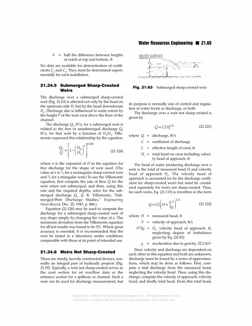
Water Resources Engineering n 21.65
b = half the difference between lengthsof notch at top and bottom, ft
No data are available for determination of coeffi-cients C2 and C3. They must be determined experi-mentally for each installation.
21.34.5 Submerged Sharp-CrestedWeirs
The discharge over a submerged sharp-crestedweir (Fig. 21.63) is affected not only by the head onthe upstream side H1 but by the head downstreamH2. Discharge also is influenced to some extent bythe height P of the weir crest above the floor of thechannel.
The discharge Qs, ft3/s, for a submerged weir is
related to the free or unsubmerged discharge Q,ft3/s, for that weir by a function of H2/H1. Ville-monte expressed this relationship by the equation
(21.120)
where n is the exponent of H in the equation forfree discharge for the shape of weir used. (Thevalue of n is 3/2 for a rectangular sharp-crested weirand 5/2 for a triangular weir.) To use the Villemonteequation, first compute the rate of flow Q for theweir when not submerged, and then, using thisrate and the required depths, solve for the sub-merged discharge Qs. (J. R. Villemonte, “Sub-merged-Weir Discharge Studies,” EngineeringNews-Record, Dec. 25, 1947, p. 866.)
Equation (21.120) may be used to compute thedischarge for a submerged sharp-crested weir ofany shape simply by changing the value of n. Themaximum deviation from the Villemonte equationfor all test results was found to be 5%. Where greataccuracy is essential, it is recommended that theweir be tested in a laboratory under conditionscomparable with those at its point of intended use.
21.34.6 Weirs Not Sharp-Crested
These are sturdy, heavily constructed devices, nor-mally an integral part of hydraulic projects (Fig.21.59). Typically, a weir not sharp-crested serves asthe crest section for an overflow dam or theentrance section for a spillway or channel. Such aweir can be used for discharge measurement, but
Copyright (C) 1999 by The McGraw-Hill Cothis product is subject to the terms of its Lic
its purpose is normally one of control and regula-tion of water levels or discharge, or both.
The discharge over a weir not sharp-crested isgiven by
(21.121)
where Q = discharge, ft3/s
C = coefficient of discharge
L = effective length of crest, ft
Ht = total head on crest including veloci-ty head of approach, ft
The head of water producing discharge over aweir is the total of measured head H and velocityhead of approach Hν. The velocity head ofapproach is accounted for by the discharge coeffi-cient for sharp-crested weirs but must be consid-ered separately for weirs not sharp-crested. Thus,for such weirs, Eq. (21.115) is rewritten in the form
(21.122)
where H = measured head, ft
V = velocity of approach, ft/s
V2/2g = Hν, velocity head of approach, ft,neglecting degree of turbulencegiven by Eq. (21.81)
g = acceleration due to gravity, 32.2 ft/s2
Since velocity and discharge are dependent oneach other in this equation and both are unknown,discharge must be found by a series of approxima-tions, which may be done as follows: First, com-pute a trial discharge from the measured head,neglecting the velocity head. Then, using this dis-charge, compute the velocity of approach, velocityhead, and finally total head. From this total head,
Fig. 21.63 Submerged sharp-crested weir.
mpanies, Inc. All rights reserved. Use ofense Agreement. Click here to view.
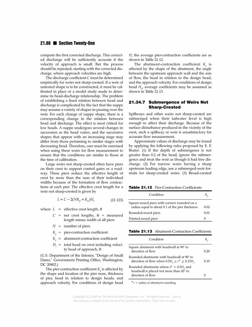
21.66 n Section Twenty-One
compute the first corrected discharge. This correct-ed discharge will be sufficiently accurate if thevelocity of approach is small. But the processshould be repeated, starting with the corrected dis-charge, where approach velocities are high.
The discharge coefficient C must be determinedempirically for weirs not sharp-crested. If a weir ofuntested shape is to be constructed, it must be cal-ibrated in place or a model study made to deter-mine its head-discharge relationship. The problemof establishing a fixed relation between head anddischarge is complicated by the fact that the nappemay assume a variety of shapes in passing over theweir. For each change of nappe shape, there is acorresponding change in the relation betweenhead and discharge. The effect is most critical forlow heads. A nappe undergoes several changes insuccession as the head varies, and the successiveshapes that appear with an increasing stage maydiffer from those pertaining to similar stages withdecreasing head. Therefore, care must be exercisedwhen using these weirs for flow measurement toensure that the conditions are similar to those atthe time of calibration.
Large weirs not sharp-crested often have pierson their crest to support control gates or a road-way. These piers reduce the effective length ofcrest by more than the sum of their individualwidths because of the formation of flow contrac-tions at each pier. The effective crest length for aweir not sharp-crested is given by
(21.123)
where L = effective crest length, ft
L′ = net crest lengths, ft = measuredlength minus width of all piers
N = number of piers
Kp = pier-contraction coefficient
Ka = abutment-contraction coefficient
Ht = total head on crest including veloci-ty head of approach, ft
(U.S. Department of the Interior, “Design of SmallDams,” Government Printing Office, Washington,DC 20402.)
The pier-contraction coefficient Kp is affected bythe shape and location of the pier nose, thicknessof pier, head in relation to design heads, andapproach velocity. For conditions of design head
Copyright (C) 1999 by The McGraw-Hill Comthis product is subject to the terms of its Lic
H, the average pier-contraction coefficients are asshown in Table 21.12.
The abutment-contraction coefficient Ka isaffected by the shape of the abutment, the anglebetween the upstream approach wall and the axisof flow, the head in relation to the design head,and the approach velocity. For conditions of designhead Hd, average coefficients may be assumed asshown in Table 21.13.
21.34.7 Submergence of Weirs NotSharp-Crested
Spillways and other weirs not sharp-crested aresubmerged when their tailwater level is highenough to affect their discharge. Because of thesurface disturbance produced in the vicinity of thecrest, such a spillway or weir is unsatisfactory foraccurate flow measurement.
Approximate values of discharge may be foundby applying the following rules proposed by E. F.Brater: (1) If the depth of submergence is notgreater than 0.2 of the head, ignore the submer-gence and treat the weir as though it had free dis-charge. (2) For narrow weirs having a sharpupstream leading edge, use a submerged-weir for-mula for sharp-crested weirs. (3) Broad-crested
Condition Kp
Square-nosed piers with corners rounded on aradius equal to about 0.1 of the pier thickness 0.02
Rounded-nosed piers 0.01
Pointed-nosed piers 0
Table 21.12 Pier-Contraction Coefficients
Condition Ka
Square abutment with headwall at 90° todirection of flow 0.20
Rounded abutments with headwall at 90° todirection of flow when 0.5Hd > r* > 0.15Hd 0.10
Rounded abutments where r* > 0.5Hd andheadwall is placed not more than 45° todirection of flow 0
*r = radius of abutment rounding.
Table 21.13 Abutment-Contraction Coefficients
panies, Inc. All rights reserved. Use ofense Agreement. Click here to view.
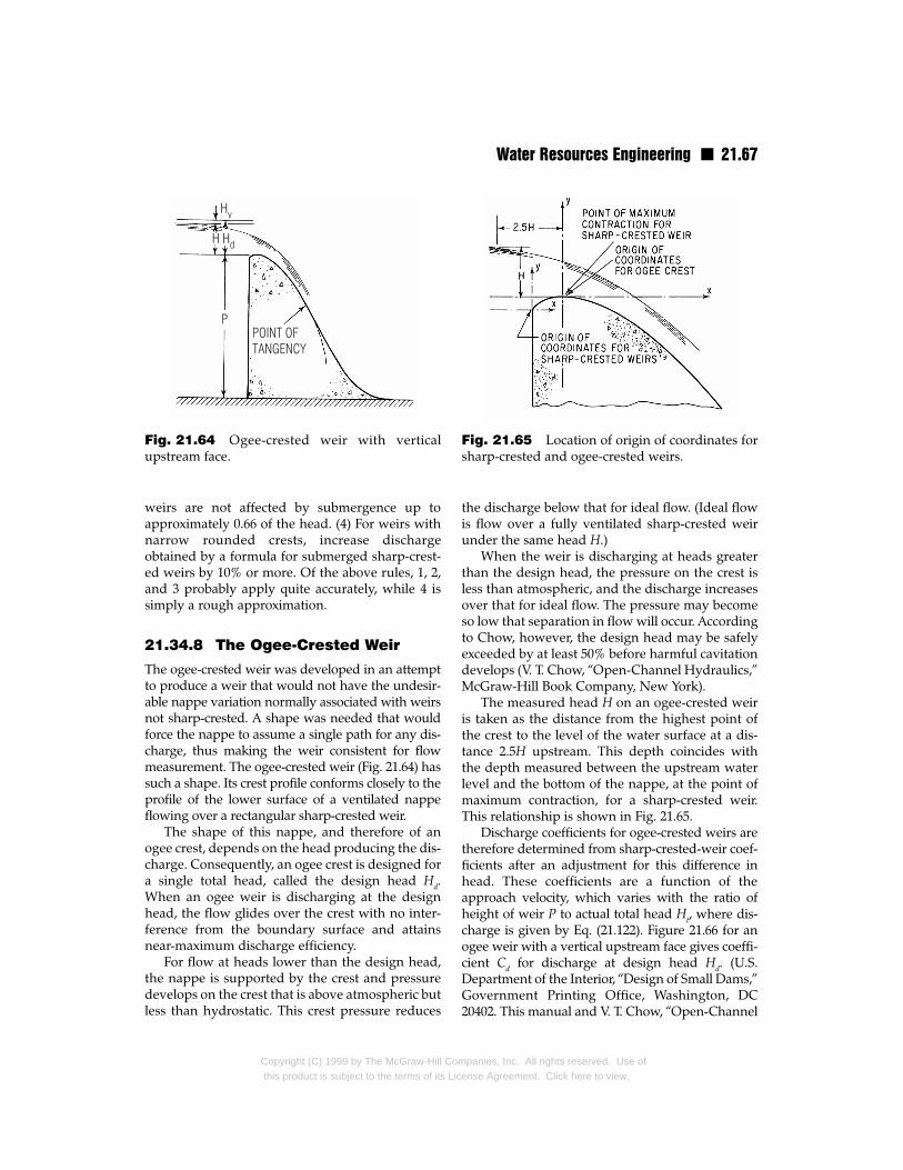
Water Resources Engineering n 21.67
weirs are not affected by submergence up toapproximately 0.66 of the head. (4) For weirs withnarrow rounded crests, increase dischargeobtained by a formula for submerged sharp-crest-ed weirs by 10% or more. Of the above rules, 1, 2,and 3 probably apply quite accurately, while 4 issimply a rough approximation.
21.34.8 The Ogee-Crested Weir
The ogee-crested weir was developed in an attemptto produce a weir that would not have the undesir-able nappe variation normally associated with weirsnot sharp-crested. A shape was needed that wouldforce the nappe to assume a single path for any dis-charge, thus making the weir consistent for flowmeasurement. The ogee-crested weir (Fig. 21.64) hassuch a shape. Its crest profile conforms closely to theprofile of the lower surface of a ventilated nappeflowing over a rectangular sharp-crested weir.
The shape of this nappe, and therefore of anogee crest, depends on the head producing the dis-charge. Consequently, an ogee crest is designed fora single total head, called the design head Hd.When an ogee weir is discharging at the designhead, the flow glides over the crest with no inter-ference from the boundary surface and attainsnear-maximum discharge efficiency.
For flow at heads lower than the design head,the nappe is supported by the crest and pressuredevelops on the crest that is above atmospheric butless than hydrostatic. This crest pressure reduces
Fig. 21.64 Ogee-crested weir with verticalupstream face.
Copyright (C) 1999 by The McGraw-Hill Cothis product is subject to the terms of its Lic
the discharge below that for ideal flow. (Ideal flowis flow over a fully ventilated sharp-crested weirunder the same head H.)
When the weir is discharging at heads greaterthan the design head, the pressure on the crest isless than atmospheric, and the discharge increasesover that for ideal flow. The pressure may becomeso low that separation in flow will occur. Accordingto Chow, however, the design head may be safelyexceeded by at least 50% before harmful cavitationdevelops (V. T. Chow, “Open-Channel Hydraulics,”McGraw-Hill Book Company, New York).
The measured head H on an ogee-crested weiris taken as the distance from the highest point ofthe crest to the level of the water surface at a dis-tance 2.5H upstream. This depth coincides withthe depth measured between the upstream waterlevel and the bottom of the nappe, at the point ofmaximum contraction, for a sharp-crested weir.This relationship is shown in Fig. 21.65.
Discharge coefficients for ogee-crested weirs aretherefore determined from sharp-crested-weir coef-ficients after an adjustment for this difference inhead. These coefficients are a function of theapproach velocity, which varies with the ratio ofheight of weir P to actual total head Ht, where dis-charge is given by Eq. (21.122). Figure 21.66 for anogee weir with a vertical upstream face gives coeffi-cient Cd for discharge at design head Hd. (U.S.Department of the Interior, “Design of Small Dams,”Government Printing Office, Washington, DC20402. This manual and V. T. Chow, “Open-Channel
Fig. 21.65 Location of origin of coordinates forsharp-crested and ogee-crested weirs.
mpanies, Inc. All rights reserved. Use ofense Agreement. Click here to view.
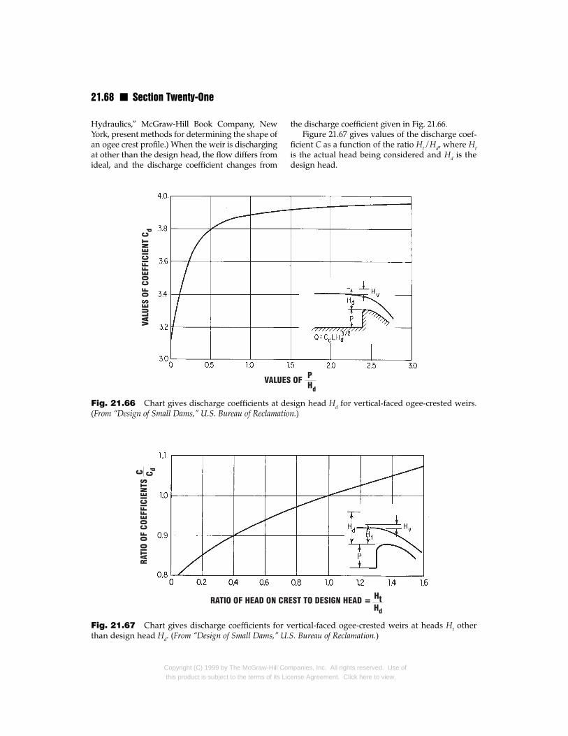
21.68 n Section Twenty-One
Hydraulics,” McGraw-Hill Book Company, NewYork, present methods for determining the shape ofan ogee crest profile.) When the weir is dischargingat other than the design head, the flow differs fromideal, and the discharge coefficient changes from
Fig. 21.66 Chart gives discharge coefficients at de(From “Design of Small Dams,” U.S. Bureau of Reclamatio
Fig. 21.67 Chart gives discharge coefficients for than design head Hd. (From “Design of Small Dams,” U
Copyright (C) 1999 by The McGraw-Hill Cothis product is subject to the terms of its Li
the discharge coefficient given in Fig. 21.66. Figure 21.67 gives values of the discharge coef-
ficient C as a function of the ratio Ht / Hd, where Htis the actual head being considered and Hd is thedesign head.
sign head Hd for vertical-faced ogee-crested weirs.n.)
vertical-faced ogee-crested weirs at heads Ht other.S. Bureau of Reclamation.)
mpanies, Inc. All rights reserved. Use ofcense Agreement. Click here to view.
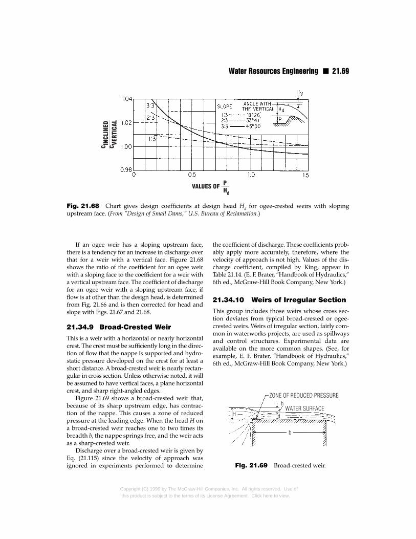
Water Resources Engineering n 21.69
Fig. 21.68 Chart gives design coefficients at design head Hd for ogee-crested weirs with slopingupstream face. (From “Design of Small Dams,” U.S. Bureau of Reclamation.)
If an ogee weir has a sloping upstream face,there is a tendency for an increase in discharge overthat for a weir with a vertical face. Figure 21.68shows the ratio of the coefficient for an ogee weirwith a sloping face to the coefficient for a weir witha vertical upstream face. The coefficient of dischargefor an ogee weir with a sloping upstream face, ifflow is at other than the design head, is determinedfrom Fig. 21.66 and is then corrected for head andslope with Figs. 21.67 and 21.68.
21.34.9 Broad-Crested Weir
This is a weir with a horizontal or nearly horizontalcrest. The crest must be sufficiently long in the direc-tion of flow that the nappe is supported and hydro-static pressure developed on the crest for at least ashort distance. A broad-crested weir is nearly rectan-gular in cross section. Unless otherwise noted, it willbe assumed to have vertical faces, a plane horizontalcrest, and sharp right-angled edges.
Figure 21.69 shows a broad-crested weir that,because of its sharp upstream edge, has contrac-tion of the nappe. This causes a zone of reducedpressure at the leading edge. When the head H ona broad-crested weir reaches one to two times itsbreadth b, the nappe springs free, and the weir actsas a sharp-crested weir.
Discharge over a broad-crested weir is given byEq. (21.115) since the velocity of approach wasignored in experiments performed to determine
Copyright (C) 1999 by The McGraw-Hill Cothis product is subject to the terms of its Li
the coefficient of discharge. These coefficients prob-ably apply more accurately, therefore, where thevelocity of approach is not high. Values of the dis-charge coefficient, compiled by King, appear inTable 21.14. (E. F. Brater, “Handbook of Hydraulics,”6th ed., McGraw-Hill Book Company, New York.)
21.34.10 Weirs of Irregular Section
This group includes those weirs whose cross sec-tion deviates from typical broad-crested or ogee-crested weirs. Weirs of irregular section, fairly com-mon in waterworks projects, are used as spillwaysand control structures. Experimental data areavailable on the more common shapes. (See, forexample, E. F. Brater, “Handbook of Hydraulics,”6th ed., McGraw-Hill Book Company, New York.)
Fig. 21.69 Broad-crested weir.
mpanies, Inc. All rights reserved. Use ofcense Agreement. Click here to view.

21.70 n Section Twenty-One
Breadth of crest of weir, ft
0.50 0.75 1.00 1.50 2.00 2.50 3.00 4.00 5.00 10.00 15.00
0.2 2.80 2.75 2.69 2.62 2.54 2.48 2.44 2.38 2.34 2.49 2.680.4 2.92 2.80 2.72 2.64 2.61 2.60 2.58 2.54 2.50 2.56 2.700.6 3.08 2.89 2.75 2.64 2.61 2.60 2.68 2.69 2.70 2.70 2.700.8 3.30 3.04 2.85 2.68 2.60 2.60 2.67 2.68 2.68 2.69 2.641.0 3.32 3.14 2.98 2.75 2.66 2.64 2.65 2.67 2.68 2.68 2.63
1.2 3.32 3.20 3.08 2.86 2.70 2.65 2.64 2.67 2.66 2.69 2.641.4 3.32 3.26 3.20 2.92 2.77 2.68 2.64 2.65 2.65 2.67 2.641.6 3.32 3.29 3.28 3.07 2.89 2.75 2.68 2.66 2.65 2.64 2.631.8 3.32 3.32 3.31 3.07 2.88 2.74 2.68 2.66 2.65 2.64 2.632.0 3.32 3.31 3.30 3.03 2.85 2.76 2.72 2.68 2.65 2.64 2.63
2.5 3.32 3.32 3.31 3.28 3.07 2.89 2.81 2.72 2.67 2.64 2.633.0 3.32 3.32 3.32 3.32 3.20 3.05 2.92 2.73 2.66 2.64 2.633.5 3.32 3.32 3.32 3.32 3.32 3.19 2.97 2.76 2.68 2.64 2.634.0 3.32 3.32 3.32 3.32 3.32 3.32 3.07 2.79 2.70 2.64 2.634.5 3.32 3.32 3.32 3.32 3.32 3.32 3.32 1.88 2.74 2.64 2.635.0 3.32 3.32 3.32 3.32 3.32 3.32 3.32 3.07 2.79 2.64 2.635.5 3.32 3.32 3.32 3.32 3.32 3.32 3.32 3.32 2.88 2.64 2.63
Table 21.14 Values of C in Q = CLH3/2 for Broad-Crested Weirs
MeasuredheadH, ft
21.35 Sediment Transfer andDeposition in OpenChannels
Sediment from open channels has many undesir-able effects: Reservoirs have a reduced useful lifebecause of loss of storage through the accumula-tion of silt. Sediment causes a hazard in navigablechannels and harbors and an increase in frequencyof flooding due to aggravation of rivers and floodchannels. Silting of arable land by flooding riversdestroys fertility when the silt originates frombank or gully erosion rather than from surface, orsoil, erosion. The cost of operating irrigation sys-tems is increased by the need for frequent dredg-ing. Water-supply facilities have increased costsbecause of the necessity of providing desiltingworks and because of the wear on mechanicalequipment, such as gates, valves, and turbines.
21.35.1 Sediment Deposition inReservoirs
Deposition of silt results when the transportingforces of a river are dissipated as the river enters a
Copyright (C) 1999 by The McGraw-Hill Cothis product is subject to the terms of its Li
body of still water, such as a reservoir. Heavier siltsizes, those forming the bed load, are deposited ina delta as the river enters calm water. The smallersilt sizes, those carried in suspension, travel fartherinto the reservoir before deposition.
This incoming water, with its load of suspendedsilt, has a specific gravity greater than that of theclear water in the reservoir and may form a density
current, rather than mixing immediately with theclear water. A density current, once formed, quicklymoves to the bottom and flows in a dense clouddown the slopes of the reservoir until it is blockedby a dam. The dense flow then spreads out in thisdeeper area, where the stilling effect of the basineventually causes deposition of the sediment.Deposits of fine sediment form about one-third ofthe volume of silt deposits in a reservoir. Much of allof this fine sediment is transported to its final loca-tion by density currents. The visible delta formed bythe coarse sediments frequently distracts attentionfrom the unseen bottom deposits of fine sediment,which are often of equal consequence.
Most reservoirs trap from 70 to almost 100% ofthe incoming sediment, depending on whetherthe reservoir is used for flood control or storage.
mpanies, Inc. All rights reserved. Use ofcense Agreement. Click here to view.

Water Resources Engineering n 21.71
Flood-control reservoirs are normally emptiedshortly after a storm, so the suspended materialsare carried out with the water before settling canoccur. This procedure reduces new deposits byalmost 30% after each storm. Storage reservoirsused for water supply or power generation pur-poses, on the other hand, normally retain anyinflow long enough for settlement of all suspend-ed matter to occur. Their discharges are regulatedto allow generation of power or to produce a uni-form flow downstream with no thought to theventing of silt-laden storm flows.
The greater part of the annual suspended siltload in a stream may be carried in a relatively shorttime. The stream runs comparatively clear duringthe remainder of the year.
Venting of much of the annual suspended siltload is feasible through the use of density currents.These currents are stable, once formed, and oftenextend to the reservoir outlet. If density currentsare observed and their time of arrival at the outletdetermined, appropriate gates can be opened andmuch of the fine sediment entering a storage reser-voir can be vented before it has time to form per-manent deposits. This venting operation canextend the life of a reservoir by many years.
Numerous phenomena can destroy a reservoir,such as loss of storage capacity by landslide andloss of the dam by earthquake, landslide, overtop-ping, or failure of materials. The most commonmanner of destruction, however, is through loss ofstorage by deposition of silt. Redemption of reser-voir capacity lost through silting is almost alwayseconomically unfeasible because of the wide distri-bution of deposits in a reservoir and the largequantity present. The most practicable means ofavoiding a loss in reservoir capacity are to preventformation of permanent deposits by taking advan-tage of density currents and to control rate of sed-iment production from eroding areas. When nei-ther can be done, sufficient storage space must beprovided in the design of the reservoir to compen-sate for depletion by silting during a reasonableeconomic lifetime.
Sediment production and its transportation toreservoirs or navigable waters cannot be prevent-ed at costs proportionate to the resulting benefits.However, nature may be economically improvedat times through a program of erosion control,reducing sediment production to less than thatnormally found under virgin conditions.
Copyright (C) 1999 by The McGraw-Hill Cothis product is subject to the terms of its Lic
The deposits of silt that form in a storage reser-voir are categorized into two distinct types: Delta
deposits, formed from the bed load, are coarse-grained, with an in-place weight of about 80 lb/ft3.Deposits produced from the suspended load arefine-grained, with an average weight of about 30lb/ft3. They constitute about one-sixth of the totalweight of sediment delivered but account forabout one-third of the volume of all deposits in astorage reservoir because of their low density. Ifsediment deposits are periodically above water,because of fluctuations in the reservoir water level,their density increases and the volume ratios givenabove for continued submergence no longer apply.
21.35.2 Prediction of Sediment-Delivery Rate
Two methods of approach are available for pre-dicting the rate of sediment accumulation in areservoir; both involve predicting the rate of sedi-ment delivery.
One approach depends on historical records ofthe silting rate for existing reservoirs and is purelyempirical. By this method, the silting records of areservoir may be used to predict either the siltingrate for that reservoir or the probable pattern ofsilt accumulation for a proposed reservoir in asimilar area. This method allows transposition ofdata from one watershed to another because themeasured annual sediment accumulation of areservoir is expressed as a rate of sediment deliv-
ery per unit area of its watershed. Of course, therate is not uniform during the year, or from year toyear, because of variations in rainfall, but it shouldaverage the computed annual amount over thelife of the project. The annual silt accumulation ina reservoir is determined by surveying exposeddeltas and taking depth soundings. The resultingvolume is adjusted to account for any silt lossthrough sluice gates or over the spillway and isthen expressed as silt delivery per square mile ofdrainage area. This silt-delivery figure is furtheradjusted for rainfall and runoff conditions, to givea figure that could reasonably be expected duringa year of average rainfall. If this adjusted figure isto be transposed to a neighboring drainage basin,adjustments should be made to account for bothsoil cover and rainfall differences between thebasins. (For a discussion of the factors upon whichthis adjustment is based, see Art. 21.39.)
mpanies, Inc. All rights reserved. Use ofense Agreement. Click here to view.
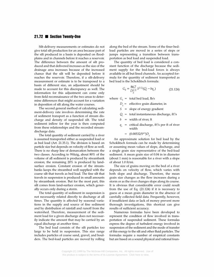
21.72 n Section Twenty-One
Silt-delivery measurements or estimates do notgive total silt production for an area because part ofthe silt produced in a basin is deposited on flood-plains and in channels before it reaches a reservoir.The difference between the amount of silt pro-duced and that delivered increases as the size of thedrainage area increases because of the increasedchance that the silt will be deposited before itreaches the reservoir. Therefore, if a silt-deliverymeasurement or estimate is to be transposed to abasin of different size, an adjustment should bemade to account for this discrepancy as well. Theinformation for this adjustment can come onlyfrom field reconnaissance of the two areas to deter-mine differences that might account for a variationin deposition of silt along the water courses.
The second general method of calculating sedi-ment-delivery rate involves determining the rateof sediment transport as a function of stream dis-charge and density of suspended silt. The totalsediment inflow for the year is then computedfrom these relationships and the recorded stream-discharge data.
The total quantity of sediment carried by a riveris assumed transported either as suspended load oras bed load (Art. 21.35.1). The division is based onparticle size but depends on velocity of flow as well.There is no sharp line of demarcation between thetwo classes. According to Witzig, about 80% of thevolume of all sediment is produced by streambankerosion; the remaining 20% is produced by land-surface erosion. Constant erosion of the stream-banks keeps the streambed well supplied with thecoarse silt that travels as bed load. The fine silt thattravels in suspension is produced in small amountsby streambank erosion. But for the most part, thissilt comes from land-surface erosion, which gener-ally occurs only during a storm.
The total quantity of sediment in suspension isnot necessarily related directly to discharge at alltimes. The quantity is affected by seasonal varia-tions in the supply and source of fine sedimentand by distribution of rainfall and runoff from thewatershed. Therefore, measurement of the sedi-ment load for a given discharge does not necessar-ily indicate the amount that may be carried by anequal discharge at another time.
The bed load consists of the silt particles toolarge to be held in suspension. This size rangeincludes particles of coarse sand, gravel, and boul-ders. The bed-load particles are moved by rolling
Copyright (C) 1999 by The McGraw-Hill Comthis product is subject to the terms of its Lic
along the bed of the stream. Some of the finer bed-load particles are moved in a series of steps orjumps representing a transition between trans-portation as bed load and suspended load.
The quantity of bed load is considered a con-stant function of the discharge because the sedi-ment supply for the bed-load forces is alwaysavailable in all but lined channels. An accepted for-mula for the quantity of sediment transported asbed load is the Schoklitsch formula:
(21.124)
where Gb = total bed load, lb/s
Dg = effective grain diameter, in
S = slope of energy gradient
Qi = total instantaneous discharge, ft3/s
b = width of river, ft
qo = critical discharge, ft3/s per ft of riverwidth
= (0.00532/S4/3)Dg
An approximate solution for bed load by theSchoklitsch formula can be made by determiningor assuming mean values of slope, discharge, anda single grain size representative of the bed-loadsediment. A mean grain size of 0.04 in in diameter(about 1 mm) is reasonable for a river with a slopeof about 1.0 ft/mi.
The size of grains moving on the bed of a riverdepends on velocity of flow, which varies withboth slope and discharge. Therefore, the meangrain size changes as the flow increases during astorm or as the river changes slope along its course.It is obvious that considerable error could resultfrom the use of Eq. (21.124) if it is necessary toguess at a mean grain diameter in the absence ofcarefully collected field data. Frequently, however,if insufficient data or lack of money prevent morethorough investigations, this shortcut can giveresults of sufficient accuracy.
Numerous formulas have been developed torepresent the condition of flow involved in trans-portation of suspended sediment. These formulasexpress the degree of turbulent energy involved insuspension of the sediment and the mode of transferof this energy to the silt and other fluid particles. Theformulas require a number of empirical constantsbut are based on a sound physical and rational foun-
panies, Inc. All rights reserved. Use ofense Agreement. Click here to view.
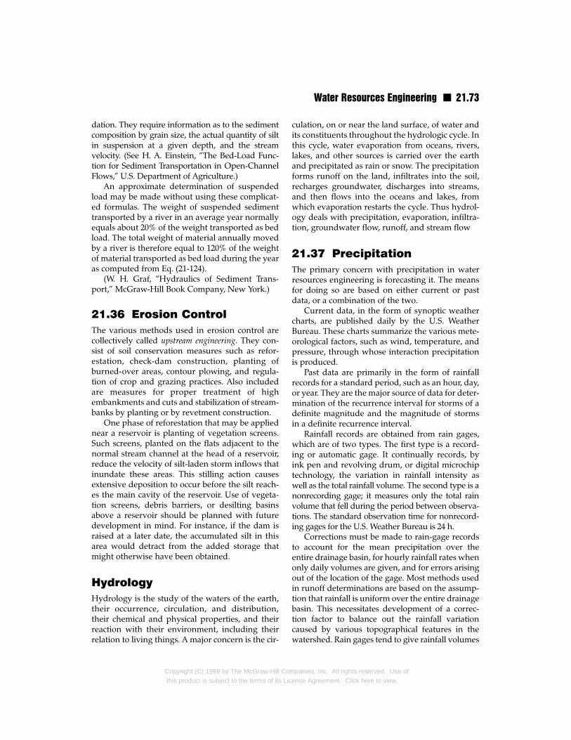
Water Resources Engineering n 21.73
dation. They require information as to the sedimentcomposition by grain size, the actual quantity of siltin suspension at a given depth, and the streamvelocity. (See H. A. Einstein, “The Bed-Load Func-tion for Sediment Transportation in Open-ChannelFlows,” U.S. Department of Agriculture.)
An approximate determination of suspendedload may be made without using these complicat-ed formulas. The weight of suspended sedimenttransported by a river in an average year normallyequals about 20% of the weight transported as bedload. The total weight of material annually movedby a river is therefore equal to 120% of the weightof material transported as bed load during the yearas computed from Eq. (21-124).
(W. H. Graf, “Hydraulics of Sediment Trans-port,” McGraw-Hill Book Company, New York.)
21.36 Erosion ControlThe various methods used in erosion control arecollectively called upstream engineering. They con-sist of soil conservation measures such as refor-estation, check-dam construction, planting ofburned-over areas, contour plowing, and regula-tion of crop and grazing practices. Also includedare measures for proper treatment of highembankments and cuts and stabilization of stream-banks by planting or by revetment construction.
One phase of reforestation that may be appliednear a reservoir is planting of vegetation screens.Such screens, planted on the flats adjacent to thenormal stream channel at the head of a reservoir,reduce the velocity of silt-laden storm inflows thatinundate these areas. This stilling action causesextensive deposition to occur before the silt reach-es the main cavity of the reservoir. Use of vegeta-tion screens, debris barriers, or desilting basinsabove a reservoir should be planned with futuredevelopment in mind. For instance, if the dam israised at a later date, the accumulated silt in thisarea would detract from the added storage thatmight otherwise have been obtained.
HydrologyHydrology is the study of the waters of the earth,their occurrence, circulation, and distribution,their chemical and physical properties, and theirreaction with their environment, including theirrelation to living things. A major concern is the cir-
Copyright (C) 1999 by The McGraw-Hill Cothis product is subject to the terms of its Lic
culation, on or near the land surface, of water andits constituents throughout the hydrologic cycle. Inthis cycle, water evaporation from oceans, rivers,lakes, and other sources is carried over the earthand precipitated as rain or snow. The precipitationforms runoff on the land, infiltrates into the soil,recharges groundwater, discharges into streams,and then flows into the oceans and lakes, fromwhich evaporation restarts the cycle. Thus hydrol-ogy deals with precipitation, evaporation, infiltra-tion, groundwater flow, runoff, and stream flow
21.37 PrecipitationThe primary concern with precipitation in waterresources engineering is forecasting it. The meansfor doing so are based on either current or pastdata, or a combination of the two.
Current data, in the form of synoptic weathercharts, are published daily by the U.S. WeatherBureau. These charts summarize the various mete-orological factors, such as wind, temperature, andpressure, through whose interaction precipitationis produced.
Past data are primarily in the form of rainfallrecords for a standard period, such as an hour, day,or year. They are the major source of data for deter-mination of the recurrence interval for storms of adefinite magnitude and the magnitude of stormsin a definite recurrence interval.
Rainfall records are obtained from rain gages,which are of two types. The first type is a record-ing or automatic gage. It continually records, byink pen and revolving drum, or digital microchiptechnology, the variation in rainfall intensity aswell as the total rainfall volume. The second type is anonrecording gage; it measures only the total rainvolume that fell during the period between observa-tions. The standard observation time for nonrecord-ing gages for the U.S. Weather Bureau is 24 h.
Corrections must be made to rain-gage recordsto account for the mean precipitation over theentire drainage basin, for hourly rainfall rates whenonly daily volumes are given, and for errors arisingout of the location of the gage. Most methods usedin runoff determinations are based on the assump-tion that rainfall is uniform over the entire drainagebasin. This necessitates development of a correc-tion factor to balance out the rainfall variationcaused by various topographical features in thewatershed. Rain gages tend to give rainfall volumes
mpanies, Inc. All rights reserved. Use ofense Agreement. Click here to view.

21.74 n Section Twenty-One
that are too small. This error is caused by the move-ment of wind around the gage, and it increases aswind velocity increases. This “windage” error ismuch more pronounced when the rain gage is nearthe top or bottom of a cliff or near other big obstruc-tions. Care must be exercised in placement of raingages to ensure accuracy.
The probable maximum precipitation is thegreatest rainfall intensity or volume that couldever be expected to occur in a specific drainagebasin. This rainfall magnitude is frequently used asthe design storm for major hydraulic structures toserve the basin when the rainfall records are shortand extrapolation to the desired design-storm fre-quency could be grossly inaccurate. The magni-tude of probable maximum precipitation is basedon simultaneous occurrence of the maximum val-ues of the meteorological factors that combine toform precipitation. The two most important factorsare wind and air-mass moisture content. An idea ofthe magnitude of the probable maximum precipi-tation can also be obtained by transposing thegreatest rainfall that has occurred in a meteorolog-ically homogeneous region. For methods for deter-mining the probable maximum precipitation, seeD. R. Maidment, “Handbook of Hydrology,”McGraw-Hill, Inc., New York.
Not all rain reaches the ground. A portion mayevaporate as it falls, while another portion may becaught on leaves, branches, and other vegetationsurfaces. This phenomenon, called interception, isa loss from a runoff standpoint since the rainevaporates and never reaches the ground. Inter-ception may be significant for small-intensitystorms occurring with little or no wind over anarea with heavy vegetation growth.
21.38 Evaporation andTranspiration
These are processes by which moisture is returnedto the atmosphere. In evaporation, water changesfrom liquid to gaseous form. In transpiration,plants give off water vapor during synthesis ofplant tissue.
Evapotranspiration, commonly termed con-
sumptive use, refers to the total evaporation fromall sources such as free water, ground, and plant-leaf surfaces. On an annual basis, the consumptiveuse may vary from 15 in/year for barren land to 35in/year for heavily forested areas and 40 in/year in
Copyright (C) 1999 by The McGraw-Hill Comthis product is subject to the terms of its Lic
tropical and subtropical regions. Evapotranspira-tion is important because, on a long-term basis, pre-cipitation minus evapotranspiration equals runoff.
Evaporation may occur from free-water, plant,or ground surfaces. Of the three, free-water sur-face evaporation is usually the most important. Itmust be considered in the design of a reservoir,especially if the reservoir is shallow, has a relative-ly large surface area, and is located in a semiarid orarid region. Evaporation is a direct function of thewind and temperature and an inverse function ofatmospheric pressure and amount of soluble solidsin the water.
The rate of evaporation is dependent on thevapor-pressure gradient between the water sur-face and the air above it. This relation is known asDalton’s law. The Meyer equation [Eq. (21.125)],developed from Dalton’s law, is one of many evap-oration formulas and is popular for making evapo-ration-rate calculations.
(21.125)
(21.126)
where E = evaporation rate, in 30-day month
C = empirical coefficient, equal to 15 forsmall, shallow pools and 11 forlarge, deep reservoirs
ew = saturation vapor pressure, in of mer-cury, corresponding to monthlymean air temperature observed atnearby stations for small bodies ofshallow water or corresponding towater temperature instead of airtemperature for large bodies of deepwater
ea = actual vapor pressure, in of mercury,in air based on monthly mean airtemperature and relative humidityat nearby stations for small bodies ofshallow water or based on informa-tion obtained about 30 ft above thewater surface for large bodies ofdeep water
w = monthly mean wind velocity, mi/hat about 30 ft above ground
ψ = wind factor
panies, Inc. All rights reserved. Use ofense Agreement. Click here to view.

Water Resources Engineering n 21.75
As an example of the evaporation that may occurfrom a large reservoir, the mean annual evapora-tion from Lake Mead is 6 ft.
Evaporation from free-water surfaces is usuallymeasured with an evaporation pan. This pan is astandard size and is located on the ground nearthe body of water whose evaporation is to bedetermined. The depth of water in this pan ischecked periodically and corrections made for fac-tors other than evaporation that may have raisedor lowered the water surface. A pan coefficient isthen applied to the measured pan evaporation toget the reservoir evaporation.
The standard evaporation pan of the NationalWeather Service, called a Class A Level Pan, is inwidespread use. It is 4 ft in diameter and 10 indeep. It is positioned 6 in above the ground. Its pancoefficient is commonly taken as 0.70, although itmay vary between 0.60 and 0.80, depending on thegeographical region. Annual evaporation from thepan ranges from 25 in in Maine and Washington to120 in along the Texas-Mexico and California-Ari-zona borders.
Evaporation rates from reservoirs may bereduced by spreading thin molecular films on thewater surface. Hexadeconal, or cetyl alcohol, is onesuch film that has been effective on small reser-voirs where there is little wind. On large reser-voirs, wind tends to push the film to the shore.Since hexadeconal is removed by wind, birds,insects, aquatic life, and biologic attrition, it mustbe applied periodically for maximum effectiveness.Hexadeconal appears to have no adverse effects oneither humans or wildlife.
Evaporation from ground surfaces is usually ofminor importance, except in arid, tropical, andsubtropical regions having high water tables andwhere it pertains to the determination of initialsoil-moisture conditions in a runoff analysis.
(D. R. Maidment, “Handbook of Hydrology,”McGraw-Hill, Inc., New York.)
21.39 RunoffThis is the residual precipitation remaining afterinterception and evapotranspiration losses havebeen deducted. It appears in surface channels,natural or manmade, whose flow is perennial orintermittent. Classified by the path taken to achannel, runoff may be surface, subsurface, orgroundwater flow.
Copyright (C) 1999 by The McGraw-Hill Cothis product is subject to the terms of its Lic
Surface flow moves across the land as overlandflow until it reaches a channel, where it continuesas channel or stream flow. After joining stream flow,it combines with the other runoff components inthe channel to form total runoff.
Subsurface flow, also known as interflow, subsur-face runoff, subsurface storm flow, and storm seepage,infiltrates only the upper soil layers without joiningthe main groundwater body. Moving laterally, itmay continue underground until it reaches a chan-nel or returns to the surface and continues as over-land flow. The time for subsurface flow to reach achannel depends on the geology of the area. Com-monly, it is assumed that subsurface flow reaches achannel during or shortly after a storm. Subsurfaceflow may be the major portion of total runoff formoderate or light rains in arid regions since surfaceflow under those conditions is reduced by unusual-ly high evaporation and infiltration.
Groundwater flow, or groundwater runoff, isthat flow supplied by deep percolation. It is theflow of the main groundwater body and requireslong periods, perhaps several years, to reach achannel. Groundwater flow is responsible for thedry-weather flow of streams and remains practi-cally constant during a storm. Groundwater flow isprimarily the concern of water-supply engineers.Surface and subsurface flow are of interest toflood-control engineers.
In practice, direct runoff and base flow are theonly two divisions of runoff used. The basis for thisclassification is travel time rather than path. Directrunoff leaves the basin during or shortly after astorm, whereas base flow from the storm may notleave the basin for months or even years.
Runoff is supplied by precipitation. The portionof precipitation that contributes entirely to directrunoff is called effective precipitation, or effective rainif the precipitation is rain. That portion of the pre-cipitation which contributes entirely to surfacerunoff is called excess precipitation, or excess rain.Thus, effective rain includes subsurface flow,whereas excess rain is only surface flow.
The two major characteristics that affect runoffare climatic and drainage-basin factors. The num-ber of factors is an indication of the complexity ofaccurately determining runoff:
1. Climatic characteristics
a. Precipitation—form (rain, hail, snow, frost,dew), intensity, duration, time distribution,
mpanies, Inc. All rights reserved. Use ofense Agreement. Click here to view.

21.76 n Section Twenty-One
seasonal distribution, areal distribution,recurrence interval, antecedent precipitation,soil moisture, direction of storm movement
b. Temperature—variation, snow storage,frozen ground during storms, extremes dur-ing precipitation
c. Wind—velocity, direction, duration
d. Humidity
e. Atmospheric pressure
f. Solar radiation
2. Drainage-basin characteristics
a. Topographic—size, shape, slope, elevation,drainage net, general location, land use andcover, lakes and other bodies of water, artifi-cial drainage, orientation, channels (size,shape of cross section, slope, roughness,length)
b. Geologic—soil type, permeability, ground-water formations, stratification
21.40 Sources of HydrologicData
The importance of exhausting all possible sourcesof hydrologic data, both published and unpub-lished, as the first step in design of a hydraulicproject cannot be overemphasized. The majorityof hydrologic data is collected and published bygovernment agencies, those of the Federal gov-ernment being the largest and most important.The principal source of precipitation data is theU.S. Weather Bureau. Its extensive system of gagessupplies complete precipitation data as well as allother types of hydrologic data. These data arecompiled and presented in monthly and yearlysummaries in the Bureau’s “Climatological Data.”In addition to the monthly and yearly summaries,special-interest items, such as rainfall intensity forvarious durations and recurrence intervals, arepublished in Weather Bureau technical papers.
Other sources are Water Bulletins of the Interna-tional Boundary Commission, the U.S. Agricultur-al Research Service, and various state and localagencies.
The principal source of runoff data is the WaterSupply Papers of the U.S. Geological Survey. Thesepapers contain records of daily flow, mean flow,yearly flow volume, extremes of flow, and statisti-
Copyright (C) 1999 by The McGraw-Hill Comthis product is subject to the terms of its Lic
cal data pertaining to the entire record. Alsoincluded in the Papers are lists of reports coveringunusually large floods and records of dischargecollected by agencies other than the U.S. Geologi-cal Survey. The Water Supply Papers are publishedyearly in 14 parts; each part is for an area whoseboundaries coincide with natural-drainage fea-tures, as shown in Fig. 21.70.
Other agencies that collect and publish stream-flow and flood records are the Corps of Engineers,TVA, International Boundary Commission, andWeather Bureau. The Corps of Engineers publishesdata on floods in which loss of life and extensiveproperty damage occurred. Less obvious sourcesof stream-flow data are water-right decrees by dis-trict courts, county records of water-right filingsand State Engineer permits, and annual reports ofvarious interstate-compact commissions.
21.41 Methods for RunoffDeterminations
The method selected to determine runoff dependson its applicability to the area of concern, the quan-tity and type of data available, the detail requiredin the final answer, and the accuracy desired.Applicability depends on the characteristics of theparticular area and the assumptions from whichthe method was developed. Quantity and type ofdata available refer to the length, detail, and com-pleteness of the hydrologic records, which may beeither precipitation or stream flow. An example ofthe variation of detail in the final result may be
Fig. 21.70 Drainage subdivisions of the UnitedStates for stream-flow records published in “WaterSupply Papers,” U.S. Geological Survey.
panies, Inc. All rights reserved. Use ofense Agreement. Click here to view.

Water Resources Engineering n 21.77
found in the determination of flood runoff. Sever-al methods yield only peak discharge; others givethe complete hydrograph. Accuracy is limited bythe cost of performing analyses and assumptionsmade in the development of a method.
The methods that follow are a convenientmeans for solving typical runoff problems encoun-tered in water resources engineering. One methodpertains to minor hydraulic structures, the secondto major hydraulic structures. A minor structure isone of low cost and of relatively minor importanceand presents small downstream damage potential.Typical examples are small highway and railroadculverts and low-capacity storm drains. Majorhydraulic structures are characterized by theirhigh cost, great importance, and large downstreamdamage potential. Typical examples of majorhydraulic structures are large reservoirs, deep cul-verts under vital highways and railways, and high-capacity storm drains and flood-control channels.
21.41.1 Method for DeterminingRunoff for Minor HydraulicStructures
The most common means for determining runoff forminor hydraulic structures is the rational formula
(21.127)
where Q = peak discharge, ft3/s
C = runoff coefficient = percentage ofrain that appears as direct runoff
I = rainfall intensity, in/h
A = drainage area, acres
The assumptions inherent in the rational formulaare:
1. The maximum rate of runoff for a particularrainfall intensity occurs if the duration of rain-fall is equal to or greater than the time of con-centration. The time of concentration is com-monly defined as the time required for water toflow from the most distant point of a drainagebasin to the point of flow measurement.
2. The maximum rate of runoff from a specificrainfall intensity whose duration is equal to orgreater than the time of concentration is direct-ly proportional to the rainfall intensity.
Copyright (C) 1999 by The McGraw-Hill Cothis product is subject to the terms of its Lic
3. The frequency of occurrence of the peak dis-charge is the same as that of the rainfall intensi-ty from which it was calculated.
4. The peak discharge per unit area decreases asthe drainage area increases, and the intensity ofrainfall decreases as its duration increases.
5. The coefficient of runoff remains constant forall storms on a given watershed.
Since these assumptions apply reasonably wellfor urbanized areas with simple drainage facilitiesof fixed dimensions and hydraulic characteristics,the rational formula has gained widespread use inthe design of drainage systems for these areas. Itssimplicity and ease of application have resulted inits being used for more complex urban systemsand rural areas where the assumptions are not soapplicable.
The rational formula is criticized for expressingrunoff as a fraction of rainfall rather than as rainfallminus losses and for combining all the complexfactors that affect runoff into a single coefficient.Although these and similar criticisms are valid, useof a more complicated formula is not justifiedbecause the time and money spent to obtain thenecessary data would not be warranted for minorhydraulic structures.
Numerous refinements have been developedfor the runoff coefficient. As an example, the LosAngeles County Flood Control District givesrunoff coefficients as a function of the soil and areatype and of the rainfall intensity for the time ofconcentration. Other similar refinements are possi-ble if the resources are available. Careful selectionof the runoff coefficient C will give values of peakrunoff consistent with project significance. Thevalues of C in Table 21.15 for urban areas are com-monly recommended design values (V. T. Chow,“Hydrologic Determination of Waterway Areas forthe Design of Drainage Structures in SmallDrainage Basins,” University of Illinois EngineeringExperimental Station Bulletin 426, 1962).
After selection of the design-storm frequency ofoccurrence, for example, a 50- or 100-year-frequencystorm, the rainfall intensity I may be determinedfrom any of a number of formulas or from a statisti-cal analysis of rainfall data if enough are available.Chow lists 24 rainfall-intensity formulas of the form
(21.128)
mpanies, Inc. All rights reserved. Use ofense Agreement. Click here to view.

21.78 n Section Twenty-One
where I = rainfall intensity, in/h
K, b, n, and n1 = respectively, coefficient, fac-tor, and exponents depend-ing on conditions that affectrainfall intensity
F = frequency of occurrence ofrainfall, years
t = duration of storm, min= time of concentration
Perhaps the most useful of these formulas is theSteel formula:
(21.129)
Type of RunoffDrainage Area Coefficient C
Business:Downtown areas 0.70 – 0.95Neighborhood areas 0.50 – 0.70
Residential:Single-family areas 0.30 – 0.50Multiunits, detached 0.40 – 0.60Multiunits, attached 0.60 – 0.75Suburban 0.25 – 0.40Apartment dwelling areas 0.50 – 0.70
Industrial:Light areas 0.50 – 0.80Heavy areas 0.60 – 0.90
Parks, cemeteries 0.10 – 0.25Playgrounds 0.20 – 0.35Railroad-yard areas 0.20 – 0.40Unimproved areas 0.10 – 0.30Streets:
Asphaltic 0.70 – 0.95Concrete 0.80 – 0.95Brick 0.70 – 0.85
Drives and walks 0.75 – 0.85Roofs 0.75 – 0.95Lawns:
Sandy soil, flat, 2% 0.05 – 0.10Sandy soil, avg, 2–7% 0.10 – 0.15Sandy soil, steep, 7% 0.15 – 0.20Heavy soil, flat, 2% 0.13 – 0.17Heavy soil, avg, 2–7% 0.18 – 0.22Heavy soil, steep, 7% 0.25 – 0.35
Table 21.15 Common Runoff Coefficients
Copyright (C) 1999 by The McGraw-Hill Comthis product is subject to the terms of its Lic
where K and b are dependent on the storm fre-quency and region of the United States (Fig. 21.71and Table 21.16).
Equation (21.129) gives the average maximumprecipitation rates for durations up to 2 h.
The time of concentration Tc at any point in adrainage system is the sum of the overland flowtime; the flow time in streets, gutters, or ditches;and the flow time in conduits. Overland flow timemay be determined from any number of formulasdeveloped for the purpose. (See D. R. Maidment,“Handbook of Hydrology,” McGraw-Hill, Inc.,New York.) The flow time in gutters, streets, ditch-es, and conduits can be determined from a calcula-tion of the average velocity using the Manningequation [Eq. (21.89)] . The time of concentration isusually expressed in minutes.
After determining the time of concentration,calculate the corresponding rainfall intensity fromeither Eq. (21.128) or Eq. (21.129), or any equivalentmethod. Then select the runoff coefficient fromTable 21.15 and determine the peak discharge fromEq. (21.127).
Since the rational formula assumes a constantuniform rainfall for the time of concentration overthe entire area, the area A must be selected so thatthis assumption applies with reasonable accuracy.Adhering to this assumption may necessitate sub-dividing the drainage area.
21.41.2 Method for DeterminingRunoff for Major HydraulicStructures
The unit-hydrograph method, pioneered in 1932 byLeRoy K. Sherman, is a convenient, widely accept-
Fig. 21.71 Regions of the United States for usewith the Steel formula.
panies, Inc. All rights reserved. Use ofense Agreement. Click here to view.
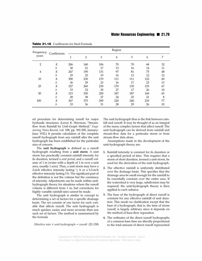
Water Resources Engineering n 21.79
RegionCoefficients
1 2 3 4 5 6 7
2 K 206 140 106 70 70 68 32b 30 21 17 13 16 14 11
4 K 247 190 131 97 81 75 48b 29 25 19 16 13 12 12
10 K 300 230 170 111 111 122 60b 36 29 23 16 17 23 13
25 K 327 260 230 170 130 155 67b 33 32 30 27 17 26 10
50 K 315 350 250 187 187 160 65b 28 38 27 24 25 21 8
100 K 367 375 290 220 240 210 77b 33 36 31 28 29 26 10
Table 21.16 Coefficients for Steel Formula
Frequency,years
ed procedure for determining runoff for majorhydraulic structures. (Leroy K. Sherman, “Stream-flow from Rainfall by Unit-Graph Method,” Engi-neering News-Record, vol. 108, pp. 501-505, January-June 1932.) It permits calculation of the completerunoff hydrograph from any rainfall after the unithydrograph has been established for the particulararea of concern.
The unit hydrograph is defined as a runoffhydrograph resulting from a unit storm. A unitstorm has practically constant rainfall intensity forits duration, termed a unit period, and a runoff vol-ume of 1 in (water with a depth of 1 in over a unitarea, usually 1 acre). Thus, a unit storm may have a2-in/h effective intensity lasting 1/2 h or a 0.2-in/heffective intensity lasting 5 h. The significant part ofthe definition is not the volume but the constancyof intensity. Adjustments can be made within unit-hydrograph theory for situations where the runoffvolume is different from 1 in, but corrections forhighly variable rainfall rates cannot be made.
The unit hydrograph is similar in concept todetermining a set of factors for a specific drainagebasin. The set consists of one factor for each vari-able that affects runoff. The unit hydrograph ismuch quicker, easier, and more accurate than anysuch set of factors. The method is summarized bythe formula
(21.130)
Copyright (C) 1999 by The McGraw-Hill Cothis product is subject to the terms of its Lic
The unit hydrograph thus is the link between rain-fall and runoff. It may be thought of as an integralof the many complex factors that affect runoff. Theunit hydrograph can be derived from rainfall andstream-flow data for a particular storm or fromstream-flow data alone.
Assumptions made in the development of theunit-hydrograph theory are:
1. Rainfall intensity is constant for its duration ora specified period of time. This requires that astorm of short duration, termed a unit storm, beused for the derivation of the unit hydrograph.
2. The effective rainfall is uniformly distributedover the drainage basin. This specifies that thedrainage area be small enough for the rainfall tobe essentially constant over the entire area. Ifthe watershed is very large, subdivision may berequired; the unit-hydrograph theory is thenapplied to each subarea.
3. The base of the hydrograph of direct runoff isconstant for any effective rainfall of unit dura-tion. This needs no clarification except that thebase of a hydrograph, that is, the time of stormrunoff, is largely arbitrary since it depends onthe method of base-flow separation.
4. The ordinates of the direct runoff hydrographsof a common base time are directly proportionalto the total amount of direct runoff represented
mpanies, Inc. All rights reserved. Use ofense Agreement. Click here to view.

21.80 n Section Twenty-One
by each hydrograph. Illustrated in Fig. 21.72,this is basically the principle of superposition orproportionality. It enables calculation of therunoff for a storm of any intensity or durationfrom a unit storm, which is of fixed intensity andduration. A given storm may be resolved into anumber of unit storms. Then, the runoff may becalculated by superimposing that number ofunit hydrographs.
5. The hydrograph of direct runoff for a givenperiod of rainfall reflects all the combined phys-ical characteristics of the basin (commonlyreferred to as the principle of time invariance).This assumption implies that the characteristicsof the drainage basin have not changed sincethe unit hydrograph was derived. Because thisapplies with varying degrees of accuracy towatersheds, the characteristics of the drainagebasin must be fixed or specified. Daily and
Fig. 21.72 Unit hydrograph (a) prepared for a uni(b) for any storm.
Copyright (C) 1999 by The McGraw-Hill Cothis product is subject to the terms of its Li
weekly variations in initial soil moisture areprobably the greatest source of error in thismethod since they are largely unknown. Man-made alterations and stream-flow conditionscan be accounted for much more easily.
For ease of manipulation, the unit hydrographis frequently expressed in histogram form as a dis-
tribution graph (Fig. 21.73), which illustrates thepercentages of total runoff that occur during suc-cessive unit periods. The ordinate for each unitperiod is the mean value of runoff for that period.
Since the unit hydrograph is derived for a unitstorm of specific duration, it may be used only forstorms divided into unit periods of that length.Usually, because of storm variations, the unit peri-od must be different from that for which the unithydrograph was derived. This requires the recal-culation of the unit hydrograph for the new unit
t storm is used to develop a composite hydrograph
mpanies, Inc. All rights reserved. Use ofcense Agreement. Click here to view.
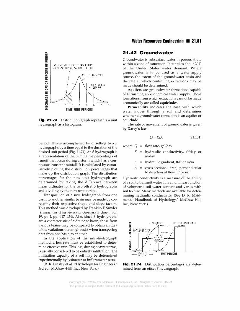
Water Resources Engineering n 21.81
period. This is accomplished by offsetting two Shydrographs by a time equal to the duration of thedesired unit period (Fig. 21.74). An S hydrograph isa representation of the cumulative percentages ofrunoff that occur during a storm which has a con-tinuous constant rainfall. It is calculated by cumu-latively plotting the distribution percentages thatmake up the distribution graph. The distributionpercentages for the new unit hydrograph aredetermined by taking the difference betweenmean ordinates for the two offset S hydrographsand dividing by the new unit period.
Transposition of a unit hydrograph from onebasin to another similar basin may be made by cor-relating their respective shape and slope factors.This method was developed by Franklin F. Snyder(Transactions of the American Geophysical Union, vol.19, pt. I, pp. 447–454). Also, since S hydrographsare a characteristic of a drainage basin, those fromvarious basins may be compared to obtain an ideaof the variations that might exist when transposingdata from one basin to another.
In the application of the unit-hydrographmethod, a loss rate must be established to deter-mine effective rain. This loss, during heavy storms,is usually considered to be entirely infiltration. Theinfiltration capacity of a soil may be determinedexperimentally by lysimeter or infiltrometer tests.
(R. K. Linsley et al., “Hydrology for Engineers,”3rd ed., McGraw-Hill, Inc., New York.)
Fig. 21.73 Distribution graph represents a unithydrograph as a histogram.
Copyright (C) 1999 by The McGraw-Hill Cothis product is subject to the terms of its Lic
21.42 GroundwaterGroundwater is subsurface water in porous stratawithin a zone of saturation. It supplies about 20%of the United States water demand. Wheregroundwater is to be used as a water-supplysource, the extent of the groundwater basin andthe rate at which continuing extractions may bemade should be determined.
Aquifers are groundwater formations capableof furnishing an economical water supply. Thoseformations from which extractions cannot be madeeconomically are called aquicludes.
Permeability indicates the ease with whichwater moves through a soil and determineswhether a groundwater formation is an aquifer oraquiclude.
The rate of movement of groundwater is givenby Darcy’s law:
(21.131)
where Q = flow rate, gal/day
K = hydraulic conductivity, ft/day orm/day
I = hydraulic gradient, ft/ft or m/m
A = cross-sectional area, perpendicularto direction of flow, ft2 or m2
Hydraulic conductivity is a measure of the abilityof a soil to transmit water. It is a nonlinear functionof volumetric soil water content and varies withsoil texture. Many methods are available for deter-mining hydraulic conductivity. (See D. R. Maid-ment, “Handbook of Hydrology,” McGraw-Hill,Inc., New York.)
Fig. 21.74 Distribution percentages are deter-mined from an offset S hydrograph.
mpanies, Inc. All rights reserved. Use ofense Agreement. Click here to view.
21.82 n Section Twenty-One
Transmissibility is another index for the rate ofgroundwater movement and equals the product ofhydraulic conductivity and the thickness of theaquifer. Transmissibility indicates for the aquifer asa whole what hydraulic conductivity indicates forthe soil.
An aquifer whose water surface is subjected toatmospheric pressure and may rise and fall withchanges in volume is a free or unconfined aquifer. Anaquifer that contains water under hydrostatic pres-sure, because of impermeable layers above andbelow it, is a confined or artesian aquifer. If a well isdrilled into an artesian aquifer, the water in thiswell will rise to a height corresponding to thehydrostatic pressure within the aquifer. Frequent-ly, this hydrostatic pressure is sufficient to causethe water to jet beyond the ground surface into theatmosphere. An artesian aquifer is analogous to alarge-capacity conduit with full flow in that extrac-tions from it cause a decrease in pressure, ratherthan a change in volume. This is in contrast to afree aquifer, where extractions cause a decrease inthe elevation of the groundwater table.
Groundwater Management n With increas-ing use being made of groundwater resources,effective groundwater management is an absolutenecessity. Adequate management should includenot only quantity but quality. Quantity manage-ment consists of effective control over extractionsand replenishment. Quality management consistsof effective control over groundwater pollutionresulting from waste disposal, recycling, poor-qual-ity replenishment waters, or other causes.
Several steps or investigations are necessary fordeveloping an effective management program. Firstis a comprehensive geologic investigation of thegroundwater basin to determine the characteristics ofthe aquifers. Second is a qualitative and quantitativehydrologic study of both surface water and ground-waters to determine historical surpluses and defi-ciencies, safe yield, and overdraft. (Safe yield is themagnitude of the annual extractions from an aquiferthat can continue indefinitely without bringing someundesirable result. Deteriorating water quality, needfor excessive pumping lifts, or infringement on thewater rights of others are examples of undesirableresults that could define safe yield. Regardless ofhow it is defined, safe yield applies only to a specificset of conditions based largely on judgment as towhat is desirable. Extractions in excess of the safe
Copyright (C) 1999 by The McGraw-Hill Comthis product is subject to the terms of its Lic
yield are termed overdrafts.) In conjunction with thehydrologic study, present and future water demandsshould be determined. A detailed water-qualitystudy should be made not only of the groundwaterwithin the basin but also of all surface waters, waste-waters, and other waters that replenish the ground-water basin. Undesirable water-quality and -quantityconditions should be identified.
Following the preceding preliminary work,alternative management plans should be formulat-ed. These management plans should consider vari-ations in the quantity of extractions; groundwaterlevels; quality, quantity, and location of artificialreplenishment; source, quantity, and quality ofwater supply; and methods of wastewater dispos-al. All alternative plans must recognize all legaland jurisdictional constraints.
The final step is the operational-economic evalu-ation of the alternatives and the selection of a rec-ommended groundwater management plan. Oper-ations and economic studies are normallyconducted by superimposing present and futureconditions in each alternative plan on historicalhydrologic conditions that occurred during a baseperiod. (A base period is a period of time, usually anumber of years, specifically chosen for detailedhydrologic analysis because conditions of watersupply and climate during the period are equivalentto a mean of long-term conditions and adequatedata for such hydrologic analysis are available.)
Economic evaluation of alternative plans shouldconsider cost of water-supply facilities, cost ofreplenishment water, cost of wastewater-disposalfacilities, cost of pumping groundwater at the vari-ous operational levels considered, and indirectwater-quality use costs, among others. (Indirectwater-quality use costs are those indirect costsincurred by water distributors and consumers as aresult of using water of different qualities. Thesecosts include increased soap costs, water softeningcosts, and costs associated with the more rapid dete-rioration of plumbing and waterworks equip-ment—all of which increase as the hardness andsalinity of the water increase.)
Operational studies should determine the mostefficient manner of joint operation of surface andgroundwater systems (conjunctive use).
Use of computers and the development of amathematical model for the groundwater basin arealmost essential because of the number of repeti-tive calculations involved.
panies, Inc. All rights reserved. Use ofense Agreement. Click here to view.
Water Resources Engineering n 21.83
Upon completion of the operational and eco-nomic studies, the most favorable managementscheme should be selected as the recommendedplan. This selection should be based not only oneconomic and operational considerations but onsocial, institutional, legal, and environmental fac-tors. The plan should be capable of being readilyimplemented, flexible enough to accommodatedifferent growth rates, financially feasible, andgenerally acceptable to the water and wastewateragencies operating in the basin.
An operating agency should be designated orformed to implement the recommended plan. Theagency should have adequate powers to control orcooperate in the control of surface-water suppliesgroundwater recharge sites, surface-water deliv-ery facilities, amount and location of groundwaterextractions, and wastewater treatment and dispos-al facilities. The operating agency should develop acomprehensive monitoring network and a datacollection and evaluation program to determinethe effectiveness of the management plan and toimplement any changes in the plan deemed neces-sary. This monitoring network may consist ofselected wells where groundwater levels andchemical characteristics are measured and certainsurface-water sampling locations where bothquantitative and qualitative factors are measured.The program should also include quantitativeevaluation of extractions, water used, wastewaterdisposed, and natural and artificial replenishment.Integration of the above data with the computermodel of the groundwater basin is an efficientmethod of evaluating the groundwater manage-ment scheme.
(“Ground Water Management,” Manual andReport on Engineering Practice, no. 40, AmericanSociety of Civil Engineers, 1987; J. Bear, “Hydraulicsof Ground Water,” N. S. Grigg, “Water ResourcesPlanning,” A. I. Kashef, “Groundwater Engineering,”R. K. Linsley et al., Hydrology for Engineers,” 3rded., McGraw-Hill Book Company, New York.)
Water SupplyA waterworks system is created or expanded tosupply a sufficient volume of water at adequatepressure from the supply source to consumers fordomestic, irrigation, industrial, fire-fighting, andsanitary purposes. A primary concern of the engi-neer is estimation of the quantity of potable water
Copyright (C) 1999 by The McGraw-Hill Cothis product is subject to the terms of its Lic
to be consumed by the community since the engi-neer must design adequately sized components ofthe water-supply system. Water-supply facilitiesconsist of collection, storage, transmission, pump-ing, distribution, and treatment works.
To assure continuous service to the consumer forfire-fighting and sanitary purposes in the event of anearthquake, fire, flood, or other unforeseen emer-gency, careful consideration must be given to theselection of standby equipment and alternative sup-plies of water. Maximum protection must be given topower sources and pumps that must be available tooperate continuously during emergency conditions.A dependable supply with sufficient pressure forfighting fires considerably increases capital expendi-tures for system construction. The smaller the sys-tem, the larger the percentage of the total costchargeable to dependable fire flow.
21.43 Water ConsumptionThe size of a proposed water-supply project is usu-ally based on an average annual per capita con-sumption rate. Therefore, forecasts of populationfor the design period are of the greatest impor-tance and must be made with care to ensure thatcomponents for the project are of adequate size.Estimation of future population, however, is a verydifficult task.
Several mathematical methods are available foruse in predicting populations of cities. Some meth-ods commonly used are arithmetical increase, per-centage increase, decreasing percentage increase,graphical comparison with other cities, and theratio method of comparing a community with astate or country of which the community is a part.Great care and judgment must be exercised in pop-ulation prediction since many factors, such asindustrial development, land speculation, geo-graphical boundaries, and age of the city, maydrastically alter mathematical estimates.
The total water supply of a city is usually dis-tributed among the following four major classes ofconsumers: domestic, industrial, commercial, andpublic.
Domestic use consists of water furnished tohouses, apartments, motels, and hotels for drink-ing, bathing, washing, sanitary, culinary, andlawn-sprinkling purposes. Domestic use accountsfor between 30 and 60% (50 to 60 gal per capita perday) of total water consumption in an average city.
mpanies, Inc. All rights reserved. Use ofense Agreement. Click here to view.
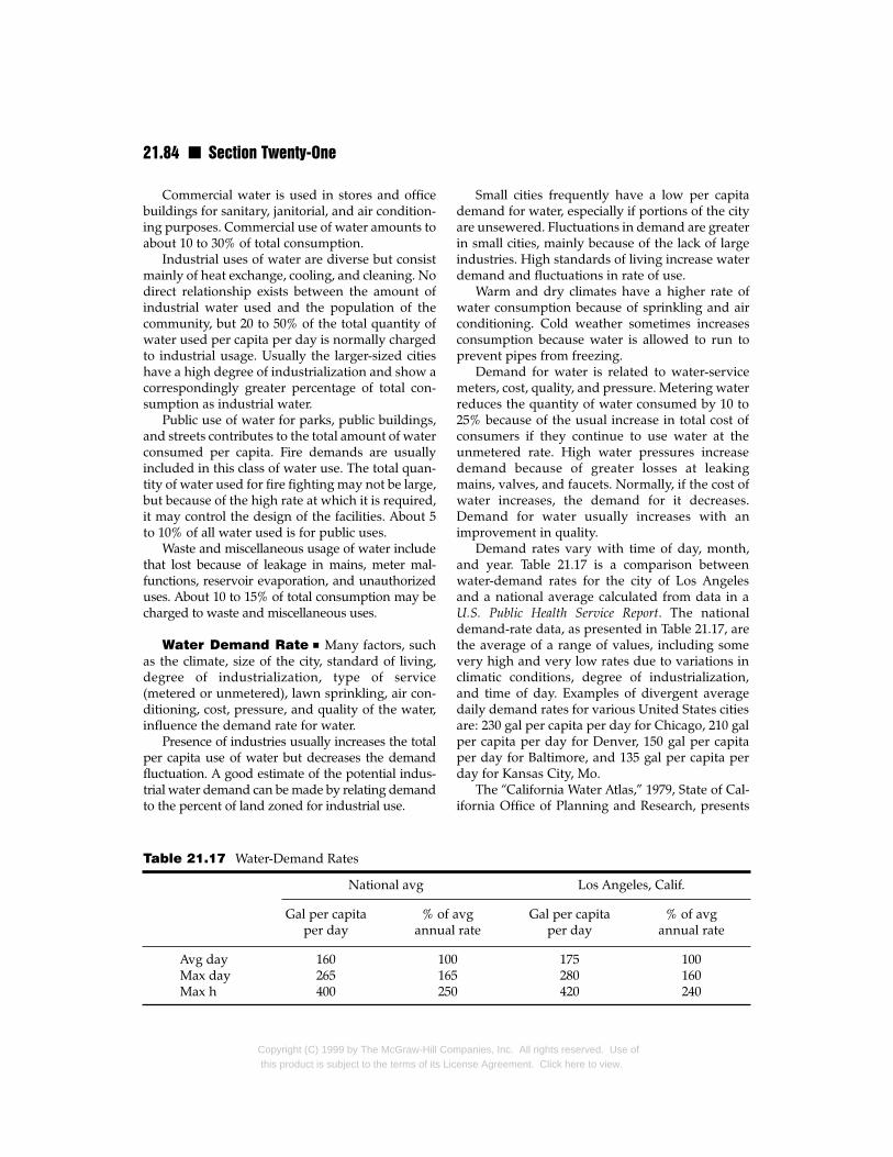
21.84 n Section Twenty-One
Commercial water is used in stores and officebuildings for sanitary, janitorial, and air condition-ing purposes. Commercial use of water amounts toabout 10 to 30% of total consumption.
Industrial uses of water are diverse but consistmainly of heat exchange, cooling, and cleaning. Nodirect relationship exists between the amount ofindustrial water used and the population of thecommunity, but 20 to 50% of the total quantity ofwater used per capita per day is normally chargedto industrial usage. Usually the larger-sized citieshave a high degree of industrialization and show acorrespondingly greater percentage of total con-sumption as industrial water.
Public use of water for parks, public buildings,and streets contributes to the total amount of waterconsumed per capita. Fire demands are usuallyincluded in this class of water use. The total quan-tity of water used for fire fighting may not be large,but because of the high rate at which it is required,it may control the design of the facilities. About 5to 10% of all water used is for public uses.
Waste and miscellaneous usage of water includethat lost because of leakage in mains, meter mal-functions, reservoir evaporation, and unauthorizeduses. About 10 to 15% of total consumption may becharged to waste and miscellaneous uses.
Water Demand Rate n Many factors, suchas the climate, size of the city, standard of living,degree of industrialization, type of service(metered or unmetered), lawn sprinkling, air con-ditioning, cost, pressure, and quality of the water,influence the demand rate for water.
Presence of industries usually increases the totalper capita use of water but decreases the demandfluctuation. A good estimate of the potential indus-trial water demand can be made by relating demandto the percent of land zoned for industrial use.
National avg
Gal per capita % of per day annua
Avg day 160 10Max day 265 16Max h 400 25
Table 21.17 Water-Demand Rates
Copyright (C) 1999 by The McGraw-Hill Cothis product is subject to the terms of its Li
Small cities frequently have a low per capitademand for water, especially if portions of the cityare unsewered. Fluctuations in demand are greaterin small cities, mainly because of the lack of largeindustries. High standards of living increase waterdemand and fluctuations in rate of use.
Warm and dry climates have a higher rate ofwater consumption because of sprinkling and airconditioning. Cold weather sometimes increasesconsumption because water is allowed to run toprevent pipes from freezing.
Demand for water is related to water-servicemeters, cost, quality, and pressure. Metering waterreduces the quantity of water consumed by 10 to25% because of the usual increase in total cost ofconsumers if they continue to use water at theunmetered rate. High water pressures increasedemand because of greater losses at leakingmains, valves, and faucets. Normally, if the cost ofwater increases, the demand for it decreases.Demand for water usually increases with animprovement in quality.
Demand rates vary with time of day, month,and year. Table 21.17 is a comparison betweenwater-demand rates for the city of Los Angelesand a national average calculated from data in aU.S. Public Health Service Report. The nationaldemand-rate data, as presented in Table 21.17, arethe average of a range of values, including somevery high and very low rates due to variations inclimatic conditions, degree of industrialization,and time of day. Examples of divergent averagedaily demand rates for various United States citiesare: 230 gal per capita per day for Chicago, 210 galper capita per day for Denver, 150 gal per capitaper day for Baltimore, and 135 gal per capita perday for Kansas City, Mo.
The “California Water Atlas,” 1979, State of Cal-ifornia Office of Planning and Research, presents
Los Angeles, Calif.
avg Gal per capita % of avgl rate per day annual rate
0 175 1005 280 1600 420 240
mpanies, Inc. All rights reserved. Use ofcense Agreement. Click here to view.

Water Resources Engineering n 21.85
average monthly demand rates for water use infour coastal and four inland cities for the period1966 to 1970. In the atlas, the effect of warm, dryclimatic conditions is indicated for each location bythe ratio of average monthly use to the annualaverage gallon per capita per day. The maximummonthly water-demand rates ranged from 119 to141% of the annual rate for the coastal cities andfrom 144 to 187% of the annual rate for the dry,inland, valley cities. Moreover, the annual demandrates for the inland areas averaged 78% higherthan those for the coastal cities. The difference isdue primarily to the great amount of lawn sprin-kling in Los Angeles. Past water-demand recordsof both the city being considered and other cities ofsimilar size, industrialization, climate, and so onshould be considered and incorporated indemand-rate projections for water systems.
The total quantity of water used for fightingfires is normally quite small, but the demand rate ishigh. The fire demand as established by the Amer-ican Insurance Association is
(21.132)
where G = fire-demand rate, gal/min
P = population, thousands
The required fire flows computed from this formulaare listed in Table 21.18. When calculating the total
gal/min MGD†
1,000 1,000 1.4 42,000 1,500 2.2 64,000 2,000 2.9 8
10,000 3,000 4.3 1017,000 4,000 5.8 1028,000 5,000 7.2 1040,000 6,000 8.6 1080,000 8,000 11.5 10
125,000 10,000 14.4 10200,000 12,000 17.3 10
* American Insurance Association.† MGD = million gallons per day; MG = million gallons.
Table 21.18 Required Fire Flow, Hydrant Spacing
Population Durath
Fire Flow
Copyright (C) 1999 by The McGraw-Hill Cothis product is subject to the terms of its Lic
flow to be used in design, fire flow should be addedto the average consumption for the maximum day.
21.44 Water-Supply SourcesThe major sources of a water supply are surfacewater and groundwater. In the past, surface sourceshave included only the commonly occurring natur-al fresh waters, such as lakes, rivers, and streams,but with rapid population expansion and increasedper capita water use associated with a higher stan-dard of living, consideration must be given todesalination and waste-water reclamation as well.
In selection of a source of supply, the variousfactors to be considered are adequacy and reliabil-ity, quality, cost, legality, and politics. The criteriaare not listed in any special order since they are, toa large extent, interdependent. Cost, however, isprobably the most important because almost anysource could be used if consumers are willing topay a high enough price. In some local areas, asincreasing demands exceed the capacity of existingsources, the increasing cost of each new supplyfocuses attention on reclamation of local suppliesof wastewater and desalination.
Adequacy of supply requires that the source belarge enough to meet the entire water demand.Total dependence on a single source, however, isfrequently undesirable, and in some cases, diversi-fication is essential for reliability. The source must
Avg area served per hydrantin high-value districts, ft*
Direct streams Engine streams
0.3 100,000 120,0000.6 90,0001.0 85,000 110,0001.8 70,000 100,0002.4 55,000 90,0003.0 40,000 85,0003.6 40,000 80,0004.8 40,000 60,0006.0 40,000 48,0007.2 40,000 40,000
, and Fire Reserve Storage*
ion, Reservestorage,
MG†
mpanies, Inc. All rights reserved. Use ofense Agreement. Click here to view.

21.86 n Section Twenty-One
also be capable of meeting demands during poweroutages and natural or created disasters. The mostdesirable supplies from a reliability standpoint, inorder, are (1) an inexhaustible supply, whetherfrom surface or groundwater, which flows by grav-ity through the distribution system; (2) a gravitysource supplemented by storage reservoirs; (3) aninexhaustible source that requires pumping; and(4) sources that require both storage and pumping.As demand increases and supplies become over-taxed, conservation practices in everyday usebecome a valuable management tool.
Quality of the source determines both accept-ability and cost; it varies considerably betweenregions. Preliminary estimates of quality can bemade by examining the source, geology, and cul-ture of the area.
Legality of supply is determined by doctrinesand principles of water rights, such as appropria-tion, riparian, and ownership rights. Appropria-tion right gives the first right priority over laterrights: “first in time means first in right.” Riparianright permits owners of land adjacent to a streamor lake to take water from that stream or lake foruse on their land. Ownership right gives alandowner possession of everything below andabove the land. Legality is especially important forgroundwater supplies or where there is transfer ofwater from one watershed to another.
A political problem with water supply existsbecause political boundaries seldom conform tonatural-drainage boundaries. This problem is espe-cially acute in extensive water-importation plans,but it even exists in varying forms for wastewaterreclamation and desalination projects.
Desalination processes are of two fundamentaltypes: those that extract salt from the water, such aselectrodialysis and ion exchange, and those thatextract water from the salt, such as distillation,freezing, and reverse osmosis. The energy cost ofthe former processes is dependent on the salt con-centration. Hence, they are used mainly for brack-ish water. The energy costs for the water-extractionprocesses are essentially independent of salinity.These processes are used for seawater conversion.Very large dual-purpose nuclear power and desali-nation plants, which take advantage of theeconomies realized by enormous facilities, havebeen proposed, but such plants are feasible onlyfor those large urban areas located on coasts. Trans-mission and pumping costs make inland use
Copyright (C) 1999 by The McGraw-Hill Comthis product is subject to the terms of its Lic
uneconomical. Although desalination may haveadvantages as a local source, it is not at present apanacea that will irrigate the deserts.
Acceptance of wastewater reclamation as awater source for direct domestic use is hindered bypublic opinion and uncertainty regarding viruses.Much effort has been expended to solve theseproblems. But until such time as they are solved,wastewater reclamation will have only limited usefor water supply. In the meantime, reclaimedwater is being used for irrigation in agriculturaland landscaping applications.
(D. W. Prasifka, “Current Trends in Water-Sup-ply Planning,” Van Nostrand Reinhold, New York.)
21.45 Quality Standards forWater
The Safe Drinking Water Act of 1974 mandatedthat nationwide standards be established to helpensure that the public receives safe water through-out the United States. National Interim PrimaryDrinking Water Standards were adopted in 1975,based largely on the 1962 U.S. Public Health Ser-vice Standards (Publication no. 956), which wereused for control of water quality for interstate car-riers. These earlier standards had been widelyadopted voluntarily by both public and privateutilities and received the immediate endorsementof the American Water Works Association as a min-imum standard for all public water supplies in theUnited States. Similar standards were developedby the World Health Organization as standards fordrinking-water quality at international ports(“International Standards for Drinking Water,”World Health Organization, Geneva, Switzerland).Heightened concern over our changing environ-ment and its health effect on water supplies was amajor cause of the change from voluntary tomandatory water-quality standards.
The Safe Drinking Water Act defines contami-
nant as any physical, chemical, biological, or radio-logical substance or matter in water. Maximum
contaminant level (MCL) indicates the maximumpermissible level of a contaminant in water that isdelivered to any user of a public water system. Theact clearly delineates between health-related qual-ity contaminants and aesthetic-related contami-nants by classifying the former as primary and thelatter as secondary contaminants.
panies, Inc. All rights reserved. Use ofense Agreement. Click here to view.

Water Resources Engineering n 21.87
Primary Standards n Tables 21.19 to 21.21 listtests and maximum contaminant levels required bythe National Interim Primary Drinking Water Regu-lations (Federal Register 40, no. 248, 5956659588,Dec. 24, 1975). Following are explanatory materialand testing frequency for compliance with the reg-ulations. Enforcement responsibility rests with theU.S. Environmental Protection Agency or withthose states electing to take primary responsibilityfor ensuring compliance with the regulations. TheEPA updates standards periodically.
Microbiological Quality n The major dan-ger associated with drinking water is the possibili-ty of its recent contamination by wastewater con-taining human excrement. Such wastewater maycontain pathogenic bacteria capable of producingtyphoid fever, cholera, or other enteric diseases.The organisms that have been most commonlyemployed as indicators of fecal pollution areEscherichia coli and the coliform group as a whole.
Table 21.19 outlines the coliform test resultsrequired to meet the MCL for bacteriological qual-ity. When organisms of the coliform group occur in
Type of contaminant
Microbiological contaminants in When using theall water systems‡
1 colony/100 mOr 4 colonies/1
samples are Or 4 colonies/1
more sampleWhen using the
Coliform shallper month
Not more thanwhen less th
Or not more tpositive whe
Turbidity in surface water 1 TU monthly asystems only
Or 5 TU average
* From “Safe Water: A Fact Book on the Safe Drinking Water Act fociation, 1979.
† TU = turbidity unit.‡ Systems using surface water or groundwater.
Table 21.19 Primary Drinking Water Standards—M
Copyright (C) 1999 by The McGraw-Hill Cothis product is subject to the terms of its Lic
three or more of the 10-mL portions of a singlestandard sample, in all five of the 100-mL portionsof a single standard sample, or exceed the givenvalues for a standard sample with the membrane-filter test, remedial measures should be undertak-en until daily samples from the same samplingpoint show at least two consecutive samples to beof satisfactory quality.
The minimum number of samples to be takenfrom the distribution system and examined eachmonth should be in accordance with the populationserved. A minimum of 1 sample should be taken inany case, with 11 samples taken for 10,000 popula-tion, 100 for 100,000 population, 300 for 1,000,000population, and 500 for 5,000,000 and over. Fordetails of methods, see “Standard Methods for theExamination of Water and Wastewater,” AmericanPublic Health Association, American Water WorksAssociation, Water Pollution Control Federation.
Turbidity n A limit on turbidity has been set asa primary contaminant because high turbidity mayinterfere with disinfection efficiency, especially invirus inactivation, and excessive particulates may
Maximum contaminant levels (MCL)†
membrane filter test:
L for the average of all monthly samples00 mL in more than one sample if less than 20
collected per month00 mL in more than 5% of the samples if 20 ors are examined per month multiple-tube fermentation test: (10-mL portions) not be present in more than 10% of the portions
one sample may have three or more portions positive an 20 samples are examined per monthhan 5% of the samples may have three or more portionsn 20 or more samples are examined per monthverage (5 TU monthly average may apply at state option)
of two consecutive days
r Non-Community Water Systems,” American Water Works Asso-
icrobiological and Turbidity*
mpanies, Inc. All rights reserved. Use ofense Agreement. Click here to view.

21.88 n Section Twenty-One
stimulate growth of microorganisms in a distribu-tion system. Daily turbidity sampling of surfacewater as it enters the distribution system isrequired, with certain exceptions in systems thatpractice disinfection and maintain an active resid-ual disinfectant in the system.
Chemical Substances n The MCL for inor-ganic and organic chemicals are listed in Table21.20. Testing for these substances to determinecompliance must be performed yearly for commu-nity water systems utilizing surface-water sourcesand every 3 years for systems using groundwater.Noncommunity water systems supplied by surfaceor groundwater must repeat the tests every 5 years.
Table 21.20 Primary Drinking Water Standards—
Type of contaminant
Inorganic chemicals in all water systems‡
ArsenicBariumCadmiumChromiumLeadMercurySeleniumSilverNitrate (as N)
Organic chemicals in surface water systems onlEndrinLindaneMethoxychlorToxaphene2, 4-D2, 4, 5-TP (Silvex)
Radiological contaminants (natural) in all waterGross alphaCombined Ra-226 and Ra-228
Radiological contaminants (synthetic) in surfacpopulations of 100,000 or more
Gross BetaTritiumStrontium-90
* From “Safe Water: A Fact Book on the Safe Drinking Water Act fociation, 1979.
† mg / L = milligrams per liter; pCi / L = picocuries per liter.‡ Systems using surface or groundwater.
Copyright (C) 1999 by The McGraw-Hill Cothis product is subject to the terms of its Li
If the routine test results indicate that the levelof any substance listed exceeds the MCL, addition-al check samples are required. For the inorganicand organic chemicals, except nitrates, if one ormore MCL are exceeded, the data are reported tothe state within 7 days and three additional sam-ples are taken at the same sampling point within 1month. If the average value of the original andthree check samples exceeds the MCL, this isreported to the state within 48 h, the public is noti-fied, and then a monitoring frequency designatedby the state should continue until the MCL has notbeen exceeded in two successive samples or until amonitoring schedule is set up as a condition to avariance, exemption, or enforcement action.
Chemicals and Radioactivity*
Maximum contaminantlevels (MCL)†
0.05 mg / L1 mg / L0.010 mg / L0.05 mg / L0.05 mg / L0.002 mg / L0.01 mg / L0.05 mg / L
10 mg / Ly
0.0002mg / L0.004 mg / L0.1 mg / L0.005 mg / L0.1 mg / L0.01 mg / L
systems‡
15 pCi / L5 pCi / L
e-water systems for
50 pCi / L20,000 pCi / L
8 pCi / L
r Non-Community Water Systems,” American Water Works Asso-
mpanies, Inc. All rights reserved. Use ofcense Agreement. Click here to view.
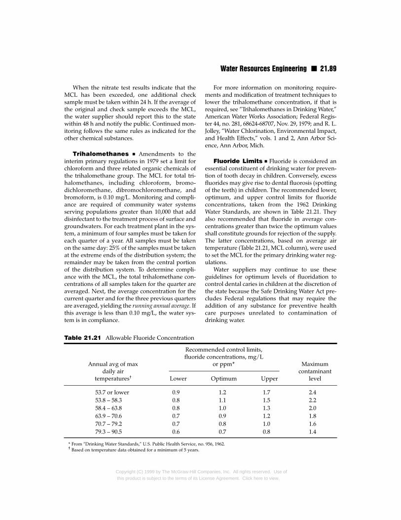
Water Resources Engineering n 21.89
When the nitrate test results indicate that theMCL has been exceeded, one additional checksample must be taken within 24 h. If the average ofthe original and check sample exceeds the MCL,the water supplier should report this to the statewithin 48 h and notify the public. Continued mon-itoring follows the same rules as indicated for theother chemical substances.
Trihalomethanes n Amendments to theinterim primary regulations in 1979 set a limit forchloroform and three related organic chemicals ofthe trihalomethane group. The MCL for total tri-halomethanes, including chloroform, bromo-dichloromethane, dibromochloromethane, andbromoform, is 0.10 mg/L. Monitoring and compli-ance are required of community water systemsserving populations greater than 10,000 that adddisinfectant to the treatment process of surface andgroundwaters. For each treatment plant in the sys-tem, a minimum of four samples must be taken foreach quarter of a year. All samples must be takenon the same day: 25% of the samples must be takenat the extreme ends of the distribution system; theremainder may be taken from the central portionof the distribution system. To determine compli-ance with the MCL, the total trihalomethane con-centrations of all samples taken for the quarter areaveraged. Next, the average concentration for thecurrent quarter and for the three previous quartersare averaged, yielding the running annual average. Ifthis average is less than 0.10 mg/L, the water sys-tem is in compliance.
Recomfluoride
Annual avg of maxdaily air
temperatures† Lower
53.7 or lower 0.953.8 – 58.3 0.858.4 – 63.8 0.863.9 – 70.6 0.770.7 – 79.2 0.779.3 – 90.5 0.6
* From “Drinking Water Standards,” U.S. Public Health Service, no† Based on temperature data obtained for a minimum of 5 years.
Table 21.21 Allowable Fluoride Concentration
Copyright (C) 1999 by The McGraw-Hill Cothis product is subject to the terms of its Lic
For more information on monitoring require-ments and modification of treatment techniques tolower the trihalomethane concentration, if that isrequired, see “Trihalomethanes in Drinking Water,”American Water Works Association; Federal Regis-ter 44, no. 281, 68624-68707, Nov. 29, 1979; and R. L.Jolley, “Water Chlorination, Environmental Impact,and Health Effects,” vols. 1 and 2, Ann Arbor Sci-ence, Ann Arbor, Mich.
Fluoride Limits n Fluoride is considered anessential constituent of drinking water for preven-tion of tooth decay in children. Conversely, excessfluorides may give rise to dental fluorosis (spottingof the teeth) in children. The recommended lower,optimum, and upper control limits for fluorideconcentrations, taken from the 1962 DrinkingWater Standards, are shown in Table 21.21. Theyalso recommended that fluoride in average con-centrations greater than twice the optimum valuesshall constitute grounds for rejection of the supply.The latter concentrations, based on average airtemperature (Table 21.21, MCL column), were usedto set the MCL for the primary drinking water reg-ulations.
Water suppliers may continue to use theseguidelines for optimum levels of fluoridation tocontrol dental caries in children at the discretion ofthe state because the Safe Drinking Water Act pre-cludes Federal regulations that may require theaddition of any substance for preventive healthcare purposes unrelated to contamination ofdrinking water.
mended control limits, concentrations, mg / L
or ppm* Maximumcontaminant
Optimum Upper level
1.2 1.7 2.41.1 1.5 2.21.0 1.3 2.00.9 1.2 1.80.8 1.0 1.60.7 0.8 1.4
. 956, 1962.
mpanies, Inc. All rights reserved. Use ofense Agreement. Click here to view.
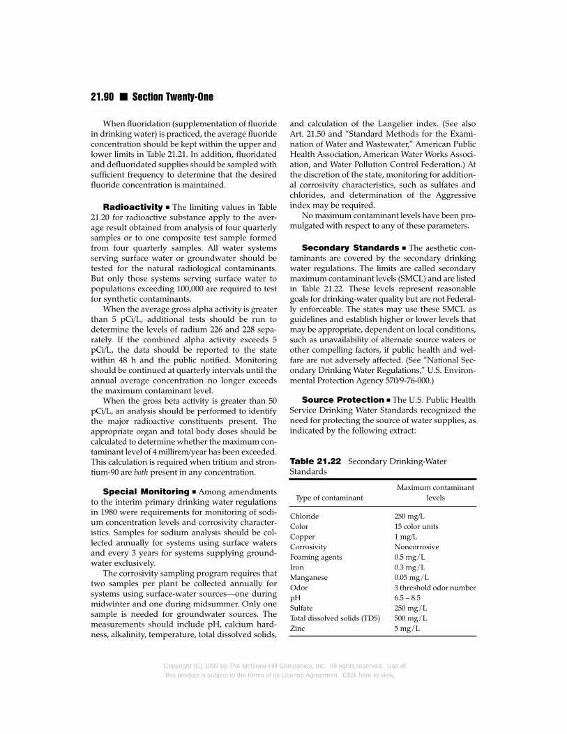
21.90 n Section Twenty-One
When fluoridation (supplementation of fluoridein drinking water) is practiced, the average fluorideconcentration should be kept within the upper andlower limits in Table 21.21. In addition, fluoridatedand defluoridated supplies should be sampled withsufficient frequency to determine that the desiredfluoride concentration is maintained.
Radioactivity n The limiting values in Table21.20 for radioactive substance apply to the aver-age result obtained from analysis of four quarterlysamples or to one composite test sample formedfrom four quarterly samples. All water systemsserving surface water or groundwater should betested for the natural radiological contaminants.But only those systems serving surface water topopulations exceeding 100,000 are required to testfor synthetic contaminants.
When the average gross alpha activity is greaterthan 5 pCi/L, additional tests should be run todetermine the levels of radium 226 and 228 sepa-rately. If the combined alpha activity exceeds 5pCi/L, the data should be reported to the statewithin 48 h and the public notified. Monitoringshould be continued at quarterly intervals until theannual average concentration no longer exceedsthe maximum contaminant level.
When the gross beta activity is greater than 50pCi/L, an analysis should be performed to identifythe major radioactive constituents present. Theappropriate organ and total body doses should becalculated to determine whether the maximum con-taminant level of 4 millirem/year has been exceeded.This calculation is required when tritium and stron-tium-90 are both present in any concentration.
Special Monitoring n Among amendmentsto the interim primary drinking water regulationsin 1980 were requirements for monitoring of sodi-um concentration levels and corrosivity character-istics. Samples for sodium analysis should be col-lected annually for systems using surface watersand every 3 years for systems supplying ground-water exclusively.
The corrosivity sampling program requires thattwo samples per plant be collected annually forsystems using surface-water sources—one duringmidwinter and one during midsummer. Only onesample is needed for groundwater sources. Themeasurements should include pH, calcium hard-ness, alkalinity, temperature, total dissolved solids,
Copyright (C) 1999 by The McGraw-Hill Comthis product is subject to the terms of its Lic
and calculation of the Langelier index. (See alsoArt. 21.50 and “Standard Methods for the Exami-nation of Water and Wastewater,” American PublicHealth Association, American Water Works Associ-ation, and Water Pollution Control Federation.) Atthe discretion of the state, monitoring for addition-al corrosivity characteristics, such as sulfates andchlorides, and determination of the Aggressiveindex may be required.
No maximum contaminant levels have been pro-mulgated with respect to any of these parameters.
Secondary Standards n The aesthetic con-taminants are covered by the secondary drinkingwater regulations. The limits are called secondarymaximum contaminant levels (SMCL) and are listedin Table 21.22. These levels represent reasonablegoals for drinking-water quality but are not Federal-ly enforceable. The states may use these SMCL asguidelines and establish higher or lower levels thatmay be appropriate, dependent on local conditions,such as unavailability of alternate source waters orother compelling factors, if public health and wel-fare are not adversely affected. (See “National Sec-ondary Drinking Water Regulations,” U.S. Environ-mental Protection Agency 570/9-76-000.)
Source Protection n The U.S. Public HealthService Drinking Water Standards recognized theneed for protecting the source of water supplies, asindicated by the following extract:
Maximum contaminantType of contaminant levels
Chloride 250 mg/LColor 15 color unitsCopper 1 mg/LCorrosivity NoncorrosiveFoaming agents 0.5 mg / LIron 0.3 mg / LManganese 0.05 mg / LOdor 3 threshold odor numberpH 6.5 – 8.5Sulfate 250 mg / LTotal dissolved solids (TDS) 500 mg / LZinc 5 mg / L
Table 21.22 Secondary Drinking-WaterStandards
panies, Inc. All rights reserved. Use ofense Agreement. Click here to view.

Water Resources Engineering n 21.91
The water supply should be obtained from the mostdesirable source feasible, and effort should be made toprevent or control pollution of the source. If thesource is not adequately protected against pollutionby natural means, the supply shall be adequately pro-tected by treatment.
Sanitary surveys shall be made of the water-supplysystem, from the source of supply to the connection ofthe customer’s service piping, to locate and correctany health hazards that might exist. The frequency ofthese surveys shall depend upon the historical need.
Adequate capacity shall be provided to meet peakdemands without development of low pressures andthe possibility of backflow of polluted water from cus-tomer piping.
Case histories and monitoring programs havebeen reported indicating that active source protec-tion can enhance water quality with minimal extraexpense. (See R. B. Pojasek, “Drinking-Water Qual-ity Enhancement through Source Protection,” AnnArbor Science Publishers, Inc., Ann Arbor, Mich.)
Water TreatmentWater is treated to remove disease-producing bac-teria, unpleasant tastes and odors, particulate andcolored matter, and hardness and to lower the lev-els of any contaminants when necessary to meetwater-quality standards. Some of the more com-mon methods of treatment are plain sedimentationand storage, coagulation-sedimentation, slow andrapid sand filtration, disinfection, and softening(see also Art. 21.51).
Long-term storage of water reduces theamount of disease-producing bacteria and particu-late matter. But economic conditions usually com-pel water purveyors to use more efficient methodsof treatment, such as those mentioned above.
21.46 SedimentationProcesses
Sedimentation or clarification is a process ofremoving particulate matter from water throughgravity settlement in a basin by reducing the flow-through velocity. Factors that affect the settlingrate of particulate matter suspended in water aresize, shape, and specific gravity of the suspendedparticles; temperature and viscosity of the water;and size and shape of the settling basin.
Copyright (C) 1999 by The McGraw-Hill Cothis product is subject to the terms of its Lic
The settling velocity νs of spherically shapedparticles in a viscous liquid can be found by use ofStokes’ law if the Reynolds number R = νρd/µ, cal-culated with ν = νs, is equal to or less than 1.
(21.133)
where νs = settling velocity of particle, m/s
g = acceleration due to gravity, m/s2
µ = absolute viscosity of the fluid, Pa⋅s
ρ1 = density of particle, g/mm3
ρ = density of fluid, g/mm3
d = particle diameter, mm
If R > 2000, Newton’s law applies:
(21.134)
where CD is the drag coefficient. Figure 21.75shows a plot of CD values vs. Reynolds numbers, tobe used in Eq. (21.134).
In the region where 1.0 < R < 2000, there is atransition from Stokes’ law to Newton’s. The set-tling velocity in this region is somewhere betweenthe values given by Newton’s law and those givenby Stokes’ law; however, no exact expression hasbeen developed to give the velocity.
Figure 21.76 shows the relationship of settlingvelocity to diameter of spherical particles with spe-cific gravity S between 1.001 and 5.0.
21.46.1 Plain Sedimentation
The ideal settling basin (Fig. 21.77) is a sedimentationtank in which flow is horizontal, velocity is constant,and concentration of particles of each size is thesame at all points of the vertical cross section at theinlet end. The basin has a volumetric capacity C,depth ho , and width B. The surface loading rate oroverflow velocity νo , equal to the settling velocity ofthe smallest particle to be completely removed, canbe determined by dividing the flow rate Q by the set-tling surface area A. For this ideal basin, the overflowvelocity therefore is νo = Q /A = Q /BLo, where Q =BhoV and Lo is the length of settling zone, V the flow-through velocity. (Usually, νo is expressed in gallonsper day per square foot of surface area.) The deten-tion time t = ho /νo = Lo /V also equals the volumetriccapacity C divided by the rate of flow Q.
mpanies, Inc. All rights reserved. Use ofense Agreement. Click here to view.
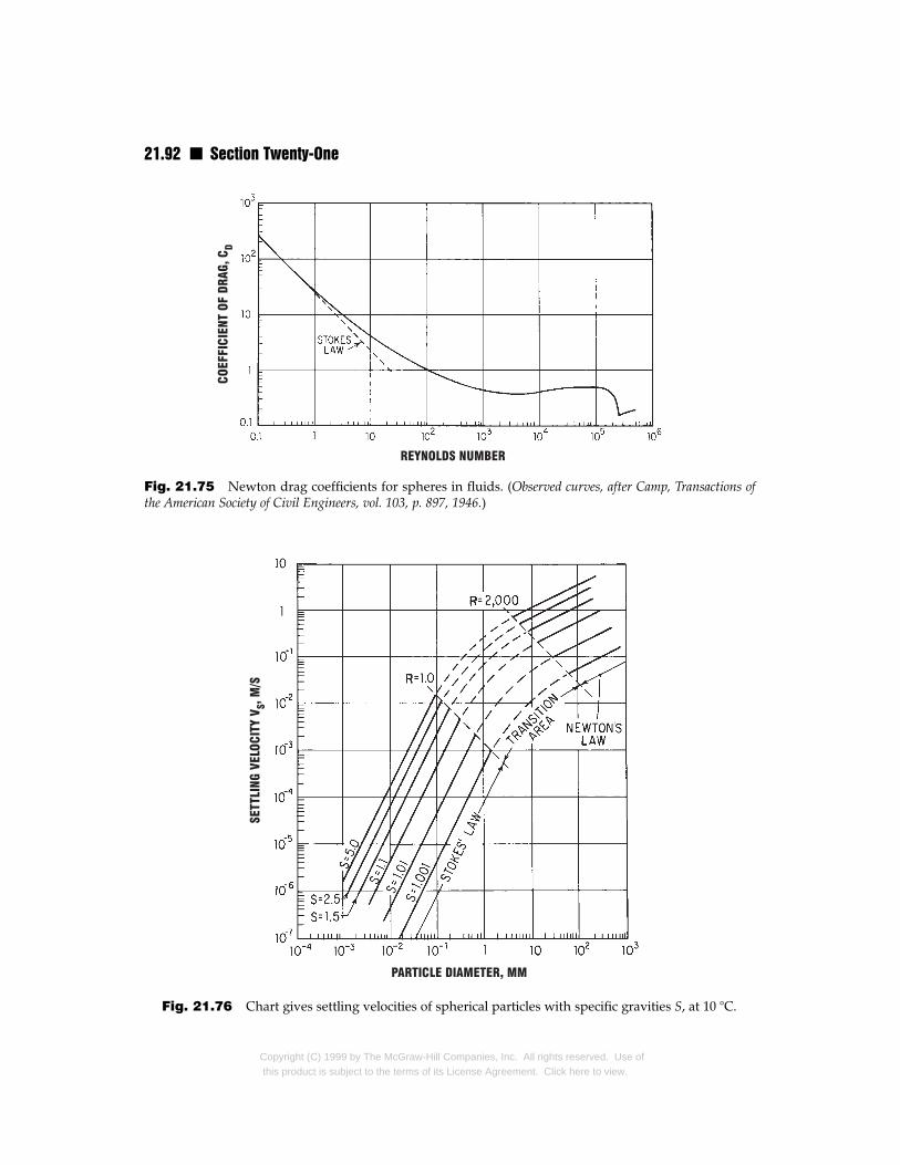
21.92 n Section Twenty-One
Fig. 21.75 Newton drag coefficients for spheres in fluids. (Observed curves, after Camp, Transactions ofthe American Society of Civil Engineers, vol. 103, p. 897, 1946.)
Fig. 21.76 Chart gives settling velocities of spherical particles with specific gravities S, at 10 °C.
Copyright (C) 1999 by The McGraw-Hill Companies, Inc. All rights reserved. Use ofthis product is subject to the terms of its License Agreement. Click here to view.

Water Resources Engineering n 21.93
Particles with a settling velocity νs > νo , andthose that enter the settling zone between f and j(at left in Fig. 21.77) with a settling velocity νs larg-er than (ν1 = h1 V/Lo) but less than νo , are removedin this basin. The particles with a settling velocityνs < ν1 that enter the settling zone between f and eare not removed in this basin.
The efficiency of a sedimentation basin is theratio of the flow-through period to the detentiontime. The flow-through period is the time requiredfor a dye, salt, or other indicator to pass throughthe basin. Settling-basin efficiencies are reduced bymany factors such as cross currents, short circuit-ing, and eddy currents. A well-designed tankshould have an efficiency of 30 to 50%.
Some design criteria for sedimentation tanks are:
Period of detention—2 to 8 h
Length-to-width ratio of flow-through channel—3:1 to 5:1
Depth of basin—10 to 25 ft (15 ft average)
Width of flow-through channel—not over 40 ft (30ft most common)
Diameter of circular tank—35 to 200 ft (most com-mon, 100 ft)
Fig. 21.77 Longitudinal section
Copyright (C) 1999 by The McGraw-Hill Cothis product is subject to the terms of its Li
Flow-through velocity—not to exceed 1.5 ft/min(most common velocity, 1.0 ft/min)
Surface loading or overflow velocity, gal per dayper ft2 of surface area—between 500 and 2000 formost settling basins
Sedimentation tanks may be built in any of avariety of shapes, for example, rectangular (Fig.21.78a) or circular (Fig. 21.78b). Multistory tanks,such as the two-story basin with a single tray in Fig.27.8c, occupy less site area than the single-storybasin. The tubular settler (Fig. 21.78d) with parallelflow upward provides very high surface areas.
(American Water Works Association and Amer-ican Society of Civil Engineers, “Water TreatmentPlant Design,” McGraw-Hill, Inc., New York; G. M.Fair, J. C. Geyer, and D. A. Okun, “Water andWastewater Engineering,” John Wiley & Sons, Inc.,New York.)
21.46.2 Coagulation-Sedimentation
To increase the settling rate and remove finelydivided particles in suspension, coagulants areadded to the water. Without coagulants, finely
through an ideal settling basin.
mpanies, Inc. All rights reserved. Use ofcense Agreement. Click here to view.

21.94 n Section Twenty-One
Fig. 21.78 Types of sedimentation tanks: (a) Rectangular settling basin. (b) Circular clarifier. (c) Two-story sedimentation basin. (d) Tubular settler.
Copyright (C) 1999 by The McGraw-Hill Companies, Inc. All rights reserved. Use ofthis product is subject to the terms of its License Agreement. Click here to view.

Water Resources Engineering n 21.95
divided particles do not settle out because of theirhigh ratio of surface area to mass and the presenceof negative charges on them. The velocity at whichdrag and gravitational forces are equal is very low,and the negative charges on the particles produceelectrostatic forces of repulsion that tend to keepthe particles separated and prevent agglomeration.When coagulating chemicals are mixed with water,however, they introduce highly charged positivenuclei that attract and neutralize the negativelycharged suspended matter.
Iron and aluminum compounds are commonlyused as coagulants because of their high positiveionic charge. The alkalinity of the water being treat-ed must be high enough for an insoluble hydroxideor hydrate of these metals to form. These insolubleflocs of iron and aluminum, which combine withthemselves and other suspended particles, precipi-tate out when a floc of sufficient size is formed.
The more common coagulants are aluminumsulfate, commonly known as alum [Al2(SO4)3.18H2O]; ferrous sulfate (FeSO4⋅7H2O); ferric chlo-ride (FeCl3); and chlorinated copperas (a mixture offerric chloride and ferrous sulfate). The type andamount of coagulant necessary to clarify a specifiedwater depend on the qualities of water to be treat-ed, such as pH, temperature, turbidity, color, andhardness. Jar tests are usually made in a laboratoryto determine the optimum amount of coagulant.
Some organic polymers are alternatives to themetallic coagulants. Polymers are long-chain, high-molecular-weight, organic polyelectrolytes. Theyare available in three types: cationic, or positivelycharged; anionic, or negatively charged; and non-ionic, or neutral in charge. Cationic polymers aregenerally the most suitable for use as primarycoagulants. Anionic polymers, however, are oftenused as flocculant aids in conjunction with an ironor aluminum salt to cause the formation of largerfloc particles. Thereby, lesser amounts of metallicsalt are needed to effect good coagulation.
Because of differences in the characteristics ofthe suspended matter found in natural waters, notall waters can be treated with equal success withthe same polymer or the same dosages. Jar testsshould be run with several dosages of the variouspolymers available to aid in selecting the materialbest suited for each water supply, considering bothcost and performance.
There are several reasons for considering theuse of polymers: increased settling rate and
Copyright (C) 1999 by The McGraw-Hill Cothis product is subject to the terms of its Li
improved filtrability of the floc, production of asmaller volume of sludge, and easier dewatering.Also, polymers have a minor effect on pH; conse-quently, the need for final pH adjustment in thefinished water may be reduced.
Process Steps n The complete clarificationprocess is usually divided into three stages: (1)rapid chemical mixing; (2) flocculation or slow stir-ring, to get the small floc to agglomerate; and (3)coagulation-sedimentation in low-flow-velocitysettling basins. Rapid chemical mixing may beaccomplished with many devices, such as mechan-ical stirrers, centrifugal pumps, and air jets. Thetime necessary for mixing ranges from a few sec-onds to 20 min. Flocculation or slow stirringincreases floc size and speeds up settling. Thespeed of the agitators must be great enough, how-ever, to cause contact between the small floc butnot so great that the larger floc is broken up. Floc-culator detention time should be in the 20- to 60-min range. The coagulation-sedimentation processtakes place in a clarifier basin nearly identical to aplain sedimentation basin. The detention periodfor a clarifier should be between 2 and 8 h.
(G. L. Culp and R. L. Culp, “New Concepts inWater Purification,” Van Nostrand Reinhold Com-pany, New York; American Water Works Associa-tion, “Water Quality and Treatment,” 4th ed., T. J.McGhee, “Water Supply and Sewerage,” R. A. Cor-bitt, “Standard Handbook of Environmental Engi-neering,” McGraw-Hill, Inc., New York.)
21.47 Filtration ProcessesPassing water through a layer of sand removesmuch of the finely divided particulate matter andsome of the larger bacteria. The filtering process hasmany components, such as physical straining,chemical and biological reactions, settling, and neu-tralization of electrostatic charges.
Direct Filtration n It is possible by use ofdirect filtration to eliminate the sedimentationstep, in some instances, for treatment of rawwaters that are low in turbidity, color, coliformorganisms, plankton, and suspended solids, suchas paper fiber. Direct filtration is a water-treatmentprocess in which raw water is not settled prior tothe filtration step. It usually includes addition of acoagulant to destabilize the colloidal particles and
mpanies, Inc. All rights reserved. Use ofcense Agreement. Click here to view.
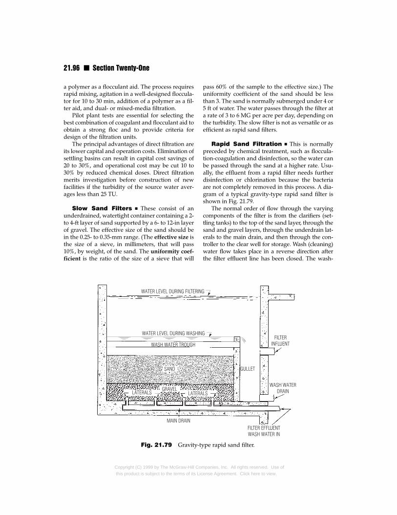
21.96 n Section Twenty-One
a polymer as a flocculant aid. The process requiresrapid mixing, agitation in a well-designed floccula-tor for 10 to 30 min, addition of a polymer as a fil-ter aid, and dual- or mixed-media filtration.
Pilot plant tests are essential for selecting thebest combination of coagulant and flocculant aid toobtain a strong floc and to provide criteria fordesign of the filtration units.
The principal advantages of direct filtration areits lower capital and operation costs. Elimination ofsettling basins can result in capital cost savings of20 to 30%, and operational cost may be cut 10 to30% by reduced chemical doses. Direct filtrationmerits investigation before construction of newfacilities if the turbidity of the source water aver-ages less than 25 TU.
Slow Sand Filters n These consist of anunderdrained, watertight container containing a 2-to 4-ft layer of sand supported by a 6- to 12-in layerof gravel. The effective size of the sand should bein the 0.25- to 0.35-mm range. (The effective size isthe size of a sieve, in millimeters, that will pass10%, by weight, of the sand. The uniformity coef-
ficient is the ratio of the size of a sieve that will
Fig. 21.79 Gravity-t
Copyright (C) 1999 by The McGraw-Hill Cothis product is subject to the terms of its Li
pass 60% of the sample to the effective size.) Theuniformity coefficient of the sand should be lessthan 3. The sand is normally submerged under 4 or5 ft of water. The water passes through the filter ata rate of 3 to 6 MG per acre per day, depending onthe turbidity. The slow filter is not as versatile or asefficient as rapid sand filters.
Rapid Sand Filtration n This is normallypreceded by chemical treatment, such as floccula-tion-coagulation and disinfection, so the water canbe passed through the sand at a higher rate. Usu-ally, the effluent from a rapid filter needs furtherdisinfection or chlorination because the bacteriaare not completely removed in this process. A dia-gram of a typical gravity-type rapid sand filter isshown in Fig. 21.79.
The normal order of flow through the varyingcomponents of the filter is from the clarifiers (set-tling tanks) to the top of the sand layer, through thesand and gravel layers, through the underdrain lat-erals to the main drain, and then through the con-troller to the clear well for storage. Wash (cleaning)water flow takes place in a reverse direction afterthe filter effluent line has been closed. The wash-
ype rapid sand filter.
mpanies, Inc. All rights reserved. Use ofcense Agreement. Click here to view.

Water Resources Engineering n 21.97
water flow is through the main drain to the laterals,from the laterals upward through the gravel andsand to the wash-water troughs. The troughs carrythe water to the gullet, which is drained to waste.
Some common design factors for rapid sand fil-ters are:
Effective grain size—0.35 to 0.55 mm
Uniformity coefficient—1.20 to 1.75
Thickness of sand layer—24 to 30 in depending ongrain size
Thickness of gravel layer—15 to 24 in
Gravel size—from 1/8 to 11/2 in
Filtration rate—2 to 4 gal/min⋅ft2 (125 to 250 MGper acre per day)
Total depth of each basin—8 to 10 ft
Maximum head loss allowed before washingsand—8 to 10 ft
Sand expansion during washing—25 to 50%
Wash-water rate—15 to 20 gal/min⋅ft2
Distance from top edge of wash-water trough totop of unexpanded sand—24 to 30 in
Length of filter runs between washings—12 to 72 h
Spacing between wash-water troughs—4 to 6 ft
Ratio of length to width of each basin—1.25 to 1.35
Rapid sand filters are operated until the partic-ulate matter and unsettled floc cover the openingsbetween the sand grains, creating a high head lossacross the filter. This high head loss slows down theflow rate and may force some of the particulatematter through the sand and gravel layers. Filtersare usually backwashed when the particulate-mat-ter concentration increases in the filter effluent orwhen the head loss reaches 8 to 10 ft. Backwashinga filter consists of forcing filtered water through thefilter from the drains upward to the wash-watertroughs. The lightweight sediment is washed fromthe sand grains by the moving water and some-times by other agitating devices, such as rakes,water sprays, and air jets. Filters must be washedthoroughly or difficulties with mud balls, bedcracking, or sand incrustation will be encountered.
Immediately after washing, filters pass water ata high rate, which produces an undertreated efflu-ent. Either manual or automatic rate control mustbe used to prevent such an occurrence. Many
Copyright (C) 1999 by The McGraw-Hill Cothis product is subject to the terms of its Lic
treatment plants control the rate of filtration byusing venturi tube devices, which throttle the filtereffluent line when there is high-velocity flow. Asclogging begins to occur in the filter, the velocity offlow in the effluent line decreases, and the ratecontroller then opens to increase the velocity.
A negative head is produced on the filter whenthe head loss across the filter is greater than thedepth of water on the sand. Negative heads canproduce a condition known as air binding, whichis caused by removal of dissolved gases from thewater and formation between sand grains of bub-bles that decrease filter capacity.
The underdrains of a filter are commonly madeof perforated pipe or porous plates. The under-drains should be arranged so that each area filtersand distributes its proportionate share of water.The ratio of total area of perforations to the total fil-ter-bed area is normally in the 0.002:1 to 0.005:1range. The diameter of the perforations variesbetween 1/4 and 3/4 in.
Wash-water troughs should be evenly spaced,and water should not have to travel more than 3 fthorizontally to get to a wash-water gutter. Thedepth of water flow in a horizontal gutter may becalculated from
(21.135)
where Q = total flow received by trough,gal/min
b = width of trough, in
y = water depth at upstream end oftrough, in
The total gutter depth can be found by adding 2 or3 in of freeboard to the calculated depth y.
Other Processes n Anthracite coal may beused in place of sand in gravity-type filters. The effec-tive grain size is greater than that of sand, thus per-mitting higher filtration rates and longer filter runs.
Dual-media, mixed-media, or deep coarse-media filters,however, may be more advantageous. They operateat the higher filtration rates of 4 to 8 gal/min⋅ft2.
A pressure filter is composed of a gravity-filtermedium enclosed in a watertight vessel. The filter-ing medium may be sand, diatomaceous earth, oranthracite coal. Pressure filters are primarily sup-plemental and are used for specialized industrialuses and for clarifying swimming pool water.
mpanies, Inc. All rights reserved. Use ofense Agreement. Click here to view.

21.98 n Section Twenty-One
Filter galleries are made up of horizontal, perfo-rated, or open-joint pipes, placed in shallow sand orgravel aquifers. Galleries typically are fed by diver-sion or pumping from streams into spreading basinswith gravel or sand bottoms. Some, however, may belocated in aquifers with high groundwater table. Thefiltered water may be pumped from the gallery orallowed to flow out one end by gravity.
(G. L. Culp and R. L. Culp, “New Concepts inWater Purification,” Van Nostrand Reinhold Com-pany, New York; American Water Works Associa-tion, “Water Quality and Treatment,” 4th ed., andAmerican Society of Civil Engineers, “Water Treat-ment Plant Design,” and T. J. McGhee, “Water Sup-ply and Sewerage,” 6th ed., McGraw-Hill BookCompany, New York; G. M. Fair, J. C. Geyer, and D.A. Okun, “Water and Wastewater Engineering,”John Wiley & Sons, Inc., New York.)
21.48 Water SofteningPresence of the bicarbonates, carbonates, sulfates,and chlorides of calcium and magnesium in watercauses hardness. Three major classifications of hard-ness are: (1) carbonate (temporary) hardness causedby bicarbonates, (2) noncarbonate (permanent)hardness, and (3) total hardness. Municipal treat-ment plants generally use either the lime-soda (pre-cipitation) process or the base-exchange (zeolite)process to reduce the hardness of the water to below100 mg/L (about 100 ppm) of CaCO3 equivalence.
In the lime-soda process, lime (CaO), hydratedlime [Ca(OH)2], and soda ash (Na2CO3) are addedto the water in sufficient quantities to reduce thehardness to an acceptable level. The amounts oflime and soda ash required for softening to a resid-ual hardness can be determined by use of chemical-equivalent weights, taking into account that com-mercial grades of lime and hydrated lime are about90 and 68% CaO, respectively. Residual hardness of50 to 100 mg/L as CaCO3 remains in the treatedwater because of the very slight solubility of bothCaCO3 and Mg(OH)2. Hardness of water is normal-ly expressed in grains per gallon (gpg) or mg/L ofCaCO3, where 1 gpg = 17.1 mg/L.
Chemical equations for the common lime-sodasoftening processes are
(21.136)
(21.137)
Copyright (C) 1999 by The McGraw-Hill Cothis product is subject to the terms of its Lic
(21.138)
(21.139)
Since the carbonate and magnesium hydroxideparticles settle out in sedimentation basins, facili-ties must be provided for particle removal and dis-posal. Deposition of CaCO3 and Mg(OH)2 on sandgrains, in clear wells, and in distribution pipes canbe prevented by recarbonation with CO2 beforesand-filter treatment.
Hardness in water can be reduced to zero bypassing the water through a base-exchange or zeo-lite material. These materials remove cations, suchas calcium and magnesium, from water andreplace them with soluble sodium and hydrogencations. Calcium can be removed from water asshown by the following reaction:
(21.140)
where Ca2+ is the calcium hardness ion removed,Na+ is the sodium ion replacing the Ca2+ in water,and R is the zeolite material. The reaction can bereversed (from right to left) by increasing the Na+
concentration to a high value, as generally is donein regeneration of the softening unit.
Sodium chloride (table salt) is commonly usedto regenerate the unit. Regeneration requiresbetween 0.3 and 0.5 lb of salt per 1000 grains ofhardness removed.
Some hardness-removal capacities per cubicfoot of base-exchange material are: natural zeo-lite—2500 to 3000 grains, synthetic zeolite—5000 to30,000 grains (1 lb = 7000 grains).
(American Water Works Association, “WaterQuality and Treatment,” 4th ed., and AmericanSociety of Civil Engineers, “Water Treatment PlantDesign,” McGraw-Hill Book Company, New York.)
21.49 Disinfection withChlorine
Chlorine in either the liquid, gas, or hypochloriteform is frequently used for destroying bacteria in
mpanies, Inc. All rights reserved. Use ofense Agreement. Click here to view.
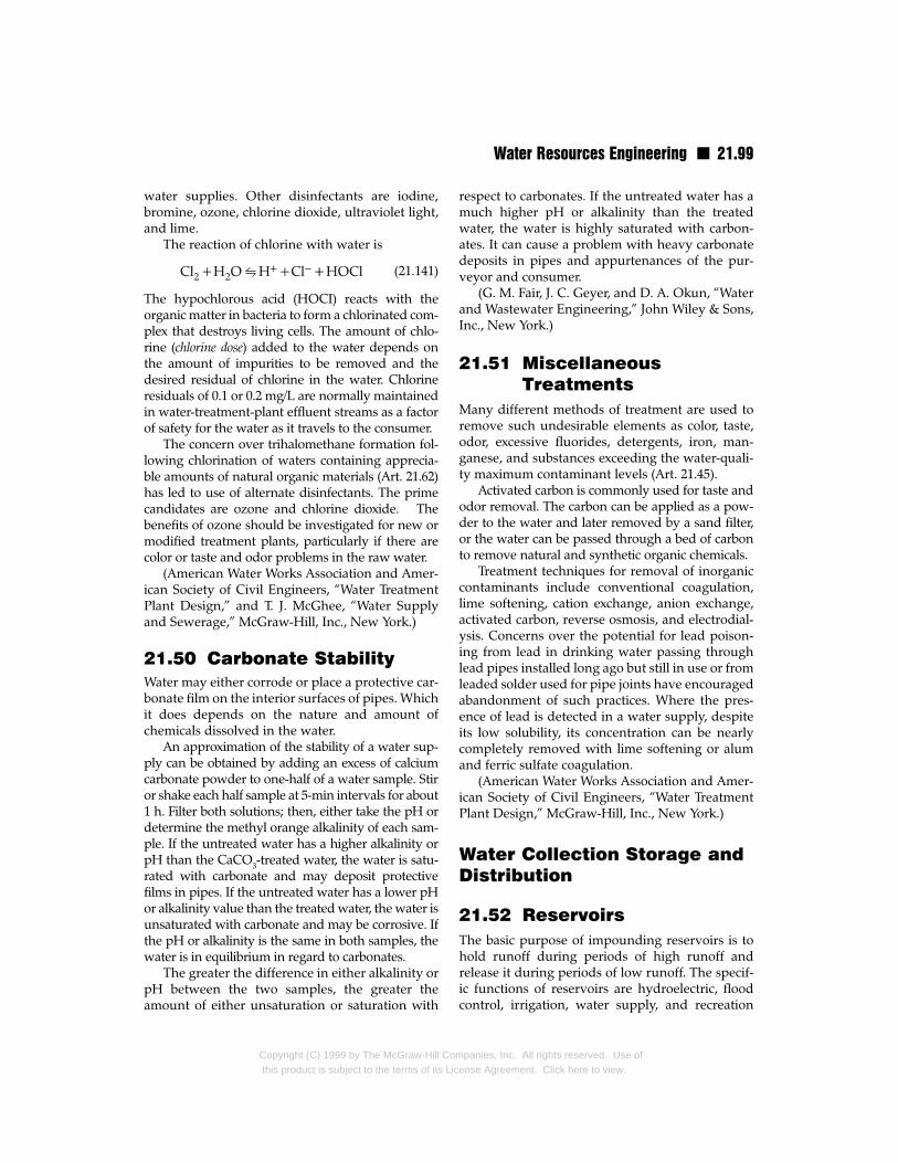
Water Resources Engineering n 21.99
water supplies. Other disinfectants are iodine,bromine, ozone, chlorine dioxide, ultraviolet light,and lime.
The reaction of chlorine with water is
(21.141)
The hypochlorous acid (HOCI) reacts with theorganic matter in bacteria to form a chlorinated com-plex that destroys living cells. The amount of chlo-rine (chlorine dose) added to the water depends onthe amount of impurities to be removed and thedesired residual of chlorine in the water. Chlorineresiduals of 0.1 or 0.2 mg/L are normally maintainedin water-treatment-plant effluent streams as a factorof safety for the water as it travels to the consumer.
The concern over trihalomethane formation fol-lowing chlorination of waters containing apprecia-ble amounts of natural organic materials (Art. 21.62)has led to use of alternate disinfectants. The primecandidates are ozone and chlorine dioxide. Thebenefits of ozone should be investigated for new ormodified treatment plants, particularly if there arecolor or taste and odor problems in the raw water.
(American Water Works Association and Amer-ican Society of Civil Engineers, “Water TreatmentPlant Design,” and T. J. McGhee, “Water Supplyand Sewerage,” McGraw-Hill, Inc., New York.)
21.50 Carbonate StabilityWater may either corrode or place a protective car-bonate film on the interior surfaces of pipes. Whichit does depends on the nature and amount ofchemicals dissolved in the water.
An approximation of the stability of a water sup-ply can be obtained by adding an excess of calciumcarbonate powder to one-half of a water sample. Stiror shake each half sample at 5-min intervals for about1 h. Filter both solutions; then, either take the pH ordetermine the methyl orange alkalinity of each sam-ple. If the untreated water has a higher alkalinity orpH than the CaCO3-treated water, the water is satu-rated with carbonate and may deposit protectivefilms in pipes. If the untreated water has a lower pHor alkalinity value than the treated water, the water isunsaturated with carbonate and may be corrosive. Ifthe pH or alkalinity is the same in both samples, thewater is in equilibrium in regard to carbonates.
The greater the difference in either alkalinity orpH between the two samples, the greater theamount of either unsaturation or saturation with
Copyright (C) 1999 by The McGraw-Hill Cothis product is subject to the terms of its Lic
respect to carbonates. If the untreated water has amuch higher pH or alkalinity than the treatedwater, the water is highly saturated with carbon-ates. It can cause a problem with heavy carbonatedeposits in pipes and appurtenances of the pur-veyor and consumer.
(G. M. Fair, J. C. Geyer, and D. A. Okun, “Waterand Wastewater Engineering,” John Wiley & Sons,Inc., New York.)
21.51 MiscellaneousTreatments
Many different methods of treatment are used toremove such undesirable elements as color, taste,odor, excessive fluorides, detergents, iron, man-ganese, and substances exceeding the water-quali-ty maximum contaminant levels (Art. 21.45).
Activated carbon is commonly used for taste andodor removal. The carbon can be applied as a pow-der to the water and later removed by a sand filter,or the water can be passed through a bed of carbonto remove natural and synthetic organic chemicals.
Treatment techniques for removal of inorganiccontaminants include conventional coagulation,lime softening, cation exchange, anion exchange,activated carbon, reverse osmosis, and electrodial-ysis. Concerns over the potential for lead poison-ing from lead in drinking water passing throughlead pipes installed long ago but still in use or fromleaded solder used for pipe joints have encouragedabandonment of such practices. Where the pres-ence of lead is detected in a water supply, despiteits low solubility, its concentration can be nearlycompletely removed with lime softening or alumand ferric sulfate coagulation.
(American Water Works Association and Amer-ican Society of Civil Engineers, “Water TreatmentPlant Design,” McGraw-Hill, Inc., New York.)
Water Collection Storage andDistribution
21.52 ReservoirsThe basic purpose of impounding reservoirs is tohold runoff during periods of high runoff andrelease it during periods of low runoff. The specif-ic functions of reservoirs are hydroelectric, floodcontrol, irrigation, water supply, and recreation
mpanies, Inc. All rights reserved. Use ofense Agreement. Click here to view.

21.100 n Section Twenty-One
(see also Art. 21.52.1). Many large reservoirs aremultipurpose, as a consequence of which the spe-cific functions may dictate conflicting design andoperating criteria. Also, equitable cost allocation ismore difficult.
Sizing of a reservoir for a project where thedemand for water is much greater than the meanstream flow is an economic balance between bene-fits and costs. A preliminary study of availablereservoir sites should be made to obtain the relativecosts for various size reservoirs. The dependableflow that can be obtained from various-size reser-voirs can be determined from the mass diagram forstream flow. An economic comparison should thenbe made of the benefits of various flows and thecosts of various reservoirs. The reservoir size thatwill give the maximum benefit should be selected.
When the demand rate is known, as is the casefor many water-supply projects, the required sizeof the reservoir can be determined directly from amass diagram of stream flow.
Fig. 21.80 Mass dia
Copyright (C) 1999 by The McGraw-Hill Cothis product is subject to the terms of its Li
The mass diagram (Fig. 21.80) is a graphical plotof total stream-flow volume against time. Theslope of the curve is the rate of flow.
Selection of the critical period of years for a masscurve depends on the function of the reservoir. Fora water-supply or hydroelectric development, min-imum flows will be critical, whereas for flood-con-trol reservoirs, maximum flows will govern.
Reservoir capacity for a certain demand can beobtained by drawing a line with a slope equal tothe demand tangent to the mass curve at thebeginning of a selected dry period, as shown bylines AB and AC in Fig. 21.80. The ordinates d ande represent the storage required to maintaindemands AB and AC.
Once a reservoir site has been selected, area-
volume curves (Fig. 21.81) are drawn to give thecharacteristics of the site. The plot of volume vs.water elevation is determined by planimeteringthe area of selected contours within the reservoirsite and multiplying by the contour interval. Aeri-
gram of stream flow.
mpanies, Inc. All rights reserved. Use ofcense Agreement. Click here to view.

Water Resources Engineering n 21.101
Fig. 21.81 Area-capacity curves for a reservoir.
al mapping has made it possible to obtain accuratecontour maps at only a fraction of the costs of oldermethods.
Another important consideration in the designof reservoirs is deposition of sediment (see Arts.21.35 and 21.52.2).
In selection of a site for a water-supply reser-voir, give special attention to water quality. If pos-sible, the watershed should be relatively uninhab-ited to reduce the amount of treatment required.(Water from practically all sources should be disin-fected in the distribution system to ensure againstpollution and contamination.) Shallow reservoirsusually give more problems with color, odor, andturbidity than deep reservoirs, particularly inwarm climates or during warm seasons of the year.Runoff heavily laden with silt and debris should bediverted from the reservoir or treated before it ismixed with the water supply. Alum is mixed intoreservoirs to reduce turbidity, and copper sulfate isused to kill vegetation.
In deep reservoirs, during the summer monthsthe upper part of the reservoir will be warmed,while below a certain level the temperature may bemany degrees cooler. The zone where the abrupttemperature change takes place, which may be onlya few feet thick, is called the thermocline. Thewaters above and below the thermocline circulate,but there is no circulation across this zone. The waterin the lower level becomes low in dissolved oxygenand develops bad tastes and odors. When the tem-
Copyright (C) 1999 by The McGraw-Hill Cothis product is subject to the terms of its Lic
perature drops in the fall, the water at the upperlevel becomes heavier than the water at the lowerlevel and the two levels become intermixed, causingbad tastes and odors in the entire reservoir. To oxi-dize organic matter and prevent poor water qualityin lower levels of reservoirs during summer months,chlorine or compressed air should be released at var-ious points on the bottom of the reservoirs.
21.52.1 Distribution Reservoirs
The two main functions of distribution reservoirsare to equalize supply and demand over periods ofvarying consumption and to supply water duringequipment failure or for fire demand. Majorsources of supply for some cities, such as NewYork, San Francisco, and Los Angeles, are large dis-tances from the city. Because of the large cost ofaqueducts, it is usually economical to size them forthe mean annual flow and provide terminal stor-age for daily and seasonal fluctuations of demand.Terminal storage is also necessary because of thepossibility of a failure along an aqueduct.
It is usually economical to have equalizingreservoirs at various points in the distribution sys-tem so that main supply lines, pumping plants, andtreatment plants can be sized for maximum dailyinstead of maximum hourly demand. During hoursof maximum demand, water flows from thesereservoirs to the consumers. When the demanddrops off, the flow refills the reservoir. A mass dia-
mpanies, Inc. All rights reserved. Use ofense Agreement. Click here to view.
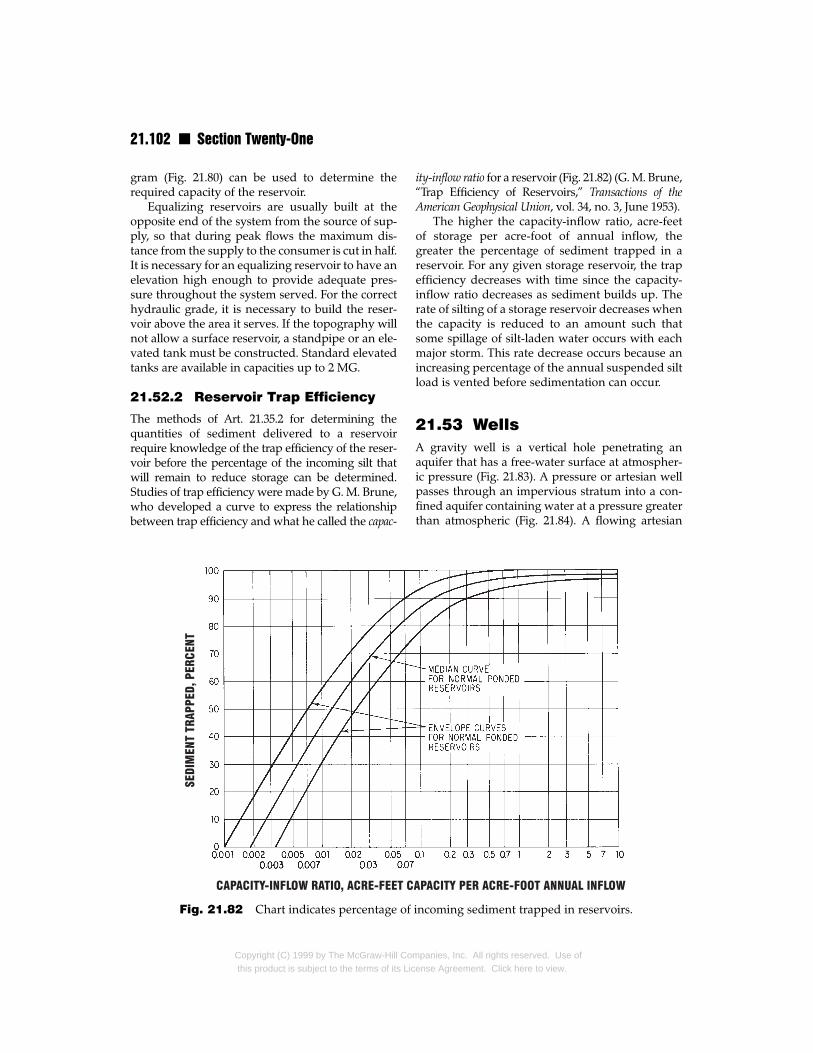
21.102 n Section Twenty-One
gram (Fig. 21.80) can be used to determine therequired capacity of the reservoir.
Equalizing reservoirs are usually built at theopposite end of the system from the source of sup-ply, so that during peak flows the maximum dis-tance from the supply to the consumer is cut in half.It is necessary for an equalizing reservoir to have anelevation high enough to provide adequate pres-sure throughout the system served. For the correcthydraulic grade, it is necessary to build the reser-voir above the area it serves. If the topography willnot allow a surface reservoir, a standpipe or an ele-vated tank must be constructed. Standard elevatedtanks are available in capacities up to 2 MG.
21.52.2 Reservoir Trap Efficiency
The methods of Art. 21.35.2 for determining thequantities of sediment delivered to a reservoirrequire knowledge of the trap efficiency of the reser-voir before the percentage of the incoming silt thatwill remain to reduce storage can be determined.Studies of trap efficiency were made by G. M. Brune,who developed a curve to express the relationshipbetween trap efficiency and what he called the capac-
Fig. 21.82 Chart indicates percentage of
Copyright (C) 1999 by The McGraw-Hill Cothis product is subject to the terms of its Li
ity-inflow ratio for a reservoir (Fig. 21.82) (G. M. Brune,“Trap Efficiency of Reservoirs,” Transactions of theAmerican Geophysical Union, vol. 34, no. 3, June 1953).
The higher the capacity-inflow ratio, acre-feetof storage per acre-foot of annual inflow, thegreater the percentage of sediment trapped in areservoir. For any given storage reservoir, the trapefficiency decreases with time since the capacity-inflow ratio decreases as sediment builds up. Therate of silting of a storage reservoir decreases whenthe capacity is reduced to an amount such thatsome spillage of silt-laden water occurs with eachmajor storm. This rate decrease occurs because anincreasing percentage of the annual suspended siltload is vented before sedimentation can occur.
21.53 WellsA gravity well is a vertical hole penetrating anaquifer that has a free-water surface at atmospher-ic pressure (Fig. 21.83). A pressure or artesian wellpasses through an impervious stratum into a con-fined aquifer containing water at a pressure greaterthan atmospheric (Fig. 21.84). A flowing artesian
incoming sediment trapped in reservoirs.
mpanies, Inc. All rights reserved. Use ofcense Agreement. Click here to view.

Water Resources Engineering n 21.103
Fig. 21.83 Gravity well in a free aquifer.
Fig. 21.84 Artesian well in a pressure aquifer.
Copyright (C) 1999 by The McGraw-Hill Companies, Inc. All rights reserved. Use ofthis product is subject to the terms of its License Agreement. Click here to view.
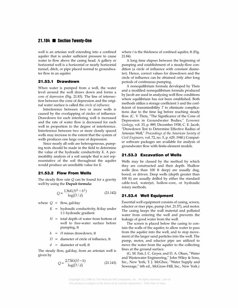
21.104 n Section Twenty-One
well is an artesian well extending into a confinedaquifer that is under sufficient pressure to causewater to flow above the casing head. A gallery orhorizontal well is a horizontal or nearly horizontaltunnel, ditch, or pipe placed normal to groundwa-ter flow in an aquifer.
21.53.1 Drawdown
When water is pumped from a well, the waterlevel around the well draws down and forms acone of depression (Fig. 21.83). The line of intersec-tion between the cone of depression and the origi-nal water surface is called the circle of influence.
Interference between two or more wells iscaused by the overlapping of circles of influence.Drawdown for each interfering well is increasedand the rate of water flow is decreased for eachwell in proportion to the degree of interference.Interference between two or more closely spacedwells may increase to the extent that the system ofwells produces one large cone of depression.
Since nearly all soils are heterogeneous, pump-ing tests should be made in the field to determinethe value of the hydraulic conductivity K. A per-meability analysis of a soil sample that is not rep-resentative of the soil throughout the aquiferwould produce an unreliable value for K.
21.53.2 Flow From Wells
The steady flow rate Q can be found for a gravitywell by using the Dupuit formula:
(21.142)
where Q = flow, gal/day
K = hydraulic conductivity, ft/day under1:1 hydraulic gradient
H = total depth of water from bottom ofwell to free-water surface beforepumping, ft
h = H minus drawdown, ft
D = diameter of circle of influence, ft
d = diameter of well, ft
The steady flow, gal/day, from an artesian well isgiven by
(21.143)
Copyright (C) 1999 by The McGraw-Hill Comthis product is subject to the terms of its Lic
where t is the thickness of confined aquifer, ft (Fig.21.84).
A long time elapses between the beginning ofpumping and establishment of a steady-flow con-dition (a circle of influence with constant diame-ter). Hence, correct values for drawdown and thecircle of influence can be obtained only after longperiods of continuous pumping.
A nonequilibrium formula developed by Theisand a modified nonequilibrium formula producedby Jacob are used in analyzing well flow conditionswhere equilibrium has not been established. Bothmethods utilize a storage coefficient S and the coef-ficient of transmissibility T to eliminate complica-tions due to the time lag before reaching steadyflow. (C. V. Theis, “The Significance of the Cone ofDepression in Groundwater Bodies,” EconomicGeology, vol. 33, p. 889, December 1938; C. E. Jacob,“Drawdown Test to Determine Effective Radius ofArtesian Well,” Proceedings of the American Society ofCivil Engineers, vol. 72, no. 5, p. 629, 1940.) Comput-er software packages are available for analysis ofgroundwater flow with finite-element models.
21.53.3 Excavation of Wells
Wells may be classed by the method by whichthey are constructed and their depth. Shallowwells (less than 100 ft deep) are usually dug,bored, or driven. Deep wells (depth greater than100 ft) are usually drilled by either the standardcable-tool, waterjet, hollow-core, or hydraulicrotary methods.
21.53.4 Well Equipment
Essential well equipment consists of casing, screen,eductor or riser pipe, pump (Art. 21.57), and motor.The casing keeps the wall material and pollutedwater from entering the well and prevents theleakage of good water from the well.
The screen is placed below the casing to con-tain the walls of the aquifer, to allow water to passfrom the aquifer into the well, and to stop move-ment of the larger sand particles into the well. Thepump, motor, and eductor pipe are utilized tomove the water from the aquifer to the collectinglines at the ground surface.
(G. M. Fair, J. C. Geyer, and D. A. Okun, “Waterand Wastewater Engineering,” John Wiley & Sons,Inc., New York; T. J. McGhee, “Water Supply andSewerage,” 6th ed., McGraw-Hill, Inc., New York.)
panies, Inc. All rights reserved. Use ofense Agreement. Click here to view.

Water Resources Engineering n 21.105
21.54 Water DistributionPiping
A water-distribution system should reliably providepotable water in sufficient quantity and at adequatepressure for domestic and fire-protection purposes.To provide adequate domestic service, the pressurein the main at house service connections usuallyshould not be below 45 psi. But if oversized plumb-ing is provided, 35 psi is adequate. In steep hillsideareas, the system is usually divided into several dif-ferent pressure zones, interconnected with pumpsand pressure regulators. Since each additional zonecauses increased expenses and decreased reliability,it is desirable to keep their number to a minimum.The American Water Works Association has recom-mended 60 to 75 psi as a desirable range for pres-sures; however, in areas of steep topography wherelocal elevation differences may be over 1000 ft, sucha narrow range is not practical.
House plumbing is designed to withstand amaximum pressure of between 100 and 125 psi.When the pressure in distribution lines is above125 psi, it is necessary to install pressure regulatorsat each house to prevent damage to appliances,such as water heaters and dishwashers.
21.54.1 Water for Fire Fighting
Pressure requirements for fire fighting depend onthe technique and equipment used. Four methodsof supplying fire protection are:
1. Use of mobile pumpers which take water froma hydrant. This method is used in most largecommunities that have full-time, well-trainedfire departments. The required pressure in theimmediate area of the fire is 20 psi.
2. Maintenance of adequate pressure at all timesin the distribution system to allow direct con-nection of fire hoses to hydrants. This techniqueis commonly used in small communities that donot have a full-time fire department and mobilepumpers. The pressure in the distribution sys-tem in the vicinity of a fire should be between50 and 75 psi.
3. Use of stationary fire pumps located at variouspoints in the distribution system, to boost thepressure during a fire and allow direct connec-tion of hoses to hydrants. This method is not soreliable or so widely used as the first two.
Copyright (C) 1999 by The McGraw-Hill Cothis product is subject to the terms of its Lic
4. Use of a separate high-pressure distribution sys-tem for fire protection only. There are only rareinstances in high-value districts of large citieswhere this method is used because the cost of adual distribution system is usually prohibitive.
21.54.2 Hydraulic Analysis ofDistribution Piping
Distribution systems are usually laid out on a grid-iron system with cross connections at variousintervals. Dead-end pipes should be avoidedbecause they cause water-quality problems.
Economic velocities are usually around 3 to 4 ft/s,although during fires they can be much higher. Two-and four-inch-diameter pipe can be used for shortlengths in residential areas; however, the AmericanInsurance Association (AIA) requires 6-in pipe forfire service in residential areas. Also, maximumlength between cross connections is limited to 600 ft.In high value districts, the AIA requires an 8-in pipe,with cross connection at all intersecting streets. TheAIA standards also require that gate valves be locat-ed so that no single case of pipe breakage, outsidemain arteries, requires shutting off from service anartery or more than 500 ft of pipe in high valued dis-tricts, or more than 800 ft in any area. All small dis-tribution lines branching from main arteries shouldbe equipped with valves. (“Standard Schedule forGrading Cities and Towns of the United States withReference to Their Fire Defenses and Physical Con-ditions,” American Insurance Association.)
Adequate service requires a knowledge of thehydraulic grade at many points in a distributionsystem for various flows. Several methods, basedon the following rules, have been developed foranalysis of complex networks:
1. The head loss in a conduit varies as a power ofthe flow rate.
2. The algebraic sum of all flows into and out ofany pipe junction equals zero.
3. The algebraic sum of all head losses betweenany two points is the same by any route, andthe algebraic sum of all head losses around aloop equals zero.
A convenient device for simplifying complexnetworks of various size pipes is the equivalent pipe.For a series of different size pipes or several parallelpipes, one pipe of any desired diameter and one
mpanies, Inc. All rights reserved. Use ofense Agreement. Click here to view.

21.106 n Section Twenty-One
specific length or any desired length and one spe-cific diameter can be substituted; this will give thesame head loss as the original for all flow rates ifthere are no take-outs or inputs between the twoend points. In complex networks, the equivalentpipe is used mainly to simplify calculation.
Example 21.10: Determine the equivalent 8-in-diameter pipe that will have the same loss of headas the sections of pipe from A to D in Fig. 21.85a.
First, transform pipes CD, AB, and BD intoequivalent lengths of 8-in pipe; then, transform theresulting sections into a single 8-in pipe with thesame head loss. The head loss may be calculatedfrom Eqs. (21.34d).
Assume any convenient flow through CD, say500 gal/min. Equation (21.34d) indicates that loss ofhead in 1000 ft of 6-in pipe is 32 ft and in 1000 ft of8-in pipe, 7.8 ft. Then, the equivalent length of 8-inpipe for CD is 500 × 32/7.8 = 2050 ft. Similarly, theequivalent pipe for AB should be 165 ft long, andfor BD, 420 ft long. The network of 8-in pipe isshown in Fig. 21.85b. It consists of pipe 1, 3000 +2050 = 5050 ft long, connected in parallel to pipe 2,165 + 420 = 585 ft long.
Fig. 21.85 Distribution loop (a) may bereplaced by equivalent loop (b).
Copyright (C) 1999 by The McGraw-Hill Comthis product is subject to the terms of its Lic
To reduce the parallel pipes to an equivalent 8-inpipe, assume a flow of 1000 gal/min through pipe 2.For this flow, the head loss in an 8-in pipe per 1000 ftis 29 ft. Hence the head loss in pipe 2 would be 29 ×585/1000 = 17 ft. Since the pipes are connected inparallel, the head loss in pipe 1 also must be 17 ft, or3.37 ft /1000 ft. The flow that will produce this headloss in an 8-in pipe is 310 gal/min [Eq. (21.34c)]. Theequivalent pipe, therefore, must carry 1000 + 310 =1310 gal/min with a head loss of 17 ft. For a flow of1310 gal/min, an 8-in pipe would have a head loss of48 ft in 1000 ft, according to Eq. 21.34d. For a loss of17 ft, an 8-in pipe would have to be 1000 × 17/48 =350 ft long. So the pipes between A and D in Fig.21.85a are equivalent to a single 8-in pipe 350 ft long.
Pipe Network Equations n For hydraulicanalysis of a water distribution system, it is conve-nient to represent the network by a mathematicalmodel. Generally, it is useful to include in themodel only the major elements needed for a math-ematical description of the basic network. (Formodels that are to be used for such conditions aslow pressures in a small service region, however, itmay be necessary to include all the distributionmains in the system.) The three analysis rules on p.21.105 can then be used to develop a system ofsimultaneous equations that can be solved for flowand pressure in the network.
Typically, either the Darcy-Weisbach or theHazen-Williams formula is used to relate the char-acteristics of each pipe in the system. Consequent-ly, the equations for each pipe are nonlinear. As aresult, a direct solution generally is not available.In practice, the equations are solved by an iterationprocess, in which the values of some variables areassumed to make the equations linear and then theequations are solved for the other variables. Theinitial assumptions are corrected and used todevelop new linear equations, which are solved toobtain more accurate values of the variables.
One example of this technique is the Hardy
Cross method, a controlled trial-and-error method,which was widely used before the advent of com-puters. Flows are first assumed; then consecutiveadjustments are computed to correct these assumedvalues. In most cases, sufficient accuracy can beobtained with three adjustments; however, thereare rare cases where the computed adjustments donot approach zero. In these cases, an approximatemethod must be used.
panies, Inc. All rights reserved. Use ofense Agreement. Click here to view.

Water Resources Engineering n 21.107
Assumed flows in a loop are adjusted in accor-dance with the following equation:
(21.144)
where KQn = hf = loss of head due to friction.When the Hazen-Williams equation, used in Exam-ple 21.10, is put in the form hf = KQn then K =4.727L/D4.87C1
1.85 and n = 1.85. The expressionΣnKQn-1 equals Σ(nKQn/Q). In the Hazen-Williamsformula n = 1.85 for all pipes and can therefore betaken outside the summation sign. Hence, theadjustment equation becomes
(21.145)
It is important that a consistent set of signs beused. The sign convention chosen for the follow-ing example makes clockwise flows and the lossesfrom these flows positive; counterclockwise flowsand their losses are negative.
Approaches generally used for formulating theequations for analysis of a water distribution net-work include the following:
Flow method, in which pipe flows are theunknowns.
Node method, in which pressure heads at thepipe end points are the unknowns.
Loop method, in which the energy in eachindependent loop is expressed in terms of theflows in each pipe in the loop. In turn, the actualflow in each pipe is expressed in terms of anassumed flow and a flow correction factor foreach loop.
Computer software packages are available foranalysis of networks by such methods. They canperform not only steady-state analyses of pres-sures and flows in pipe networks but also time-dependent analyses of pressure and flow underchanging system demands and of flow patternsand basic water quality.
(V. J. Zipparo and H. Hasen, “Davis’ Handbookof Applied Hydraulics,” McGraw-Hill, Inc., NewYork; AWWA, “Distribution Network Analysis forWater Utilities,” Manual of Water Supply PracticesM32, American Water Works Association, Denver,Colo.; T. M. Walski, “Analysis of Water DistributionSystems,” Van Nostrand Reinhold, New York.)
Copyright (C) 1999 by The McGraw-Hill Cothis product is subject to the terms of its Lic
21.54.3 Cover over Buried Pipes
The cover required over distribution pipesdepends on the climate, size of main, and traffic. Innorthern areas, frost penetration, which may be asdeep as 7 ft. is usually the governing factor. Infrost-free areas, a minimum of 24 in is required bythe AIA. If large mains are placed under heavytraffic, the stress produced by wheel loads shouldbe investigated.
21.54.4 Maintenance of WaterPipes
Maintenance of distribution systems involves keep-ing records, cleaning and lining pipe, finding andrepairing leaks, inspecting hydrants and valves,and many other functions necessary to eliminateproblems in operation. Valves should be inspectedannually and fire hydrants semiannually. Recordsof all inspections and repairs should be kept.
Unlined distribution pipes, after years of usage,lose much of their capacity because of corrosionand incrustations. Cleaning and lining withcement mortar restores the original capacity. Dead-end pipes should be flushed periodically to reducethe accumulation of rust and organic matter.
21.54.5 Economic Sizing ofDistribution Piping
When designing any major project, the designershould choose the most economical of numerousalternatives. Most of these alternatives can be sep-arated and studied individually. An example oftwo alternatives for a distribution system is oneserving peak hourly demands totally by pumpsand one doing it by pumps and equalizing reser-voirs. The total costs of each plan should be com-pared by an annual or present-worth cost analysis.
A method of determining minimum cost thatcan readily be adapted to many conditions is set-ting the first derivative of the total cost, taken withrespect to the variable in question, equal to zero. Inthe sizing of pipes in a distribution system suppliedby pumps, the total costs of the pipes, pumpingplant, and energy may be expressed as an equation.To find the most economical diameter of pipe, thefirst derivative of the total cost, taken with respectto the pipe diameter, should be set equal to zero.The following equation for the most economicalpipe diameter was derived in that manner:
mpanies, Inc. All rights reserved. Use ofense Agreement. Click here to view.

21.108 n Section Twenty-One
(21.146)
where D = pipe diameter, ft
f = Darcy-Weisbach friction factor
b = value of power, dollars/hp per year
Qa = average discharge, ft3/s
S = allowable unit stress in pipe, psi
a = in-place cost of pipe, dollars/pound
i = yearly fixed charges for pipeline(expressed as a fraction of total capi-tal cost)
Ha = average head on pipe, ft
21.54.6 Pipe Materials
Cast iron, steel, concrete, and plastics, such aspolyvinyl chloride, polyethylene, polybutylene, andglass-fiber-reinforced thermosetting resins, are themost common materials used in distribution pipes.Wood pipelines are still in existence, but wood israrely used in new installations. Copper, lead, zinc,brass, bronze, and plastic are materials used in smallpipes, valves, pumps, and other appurtenances.Common pipe-joint materials are: cement, sand;rubber, plastic, and sulfur compounds.
Cast iron is the most common material for citywater mains. Standard sizes range from 2 to 24 inin diameter. Cast iron is resistant to corrosion andusually has good hydraulic characteristics. If it iscement-lined, the Hazen-Williams C value may beas high as 145. In unlined pipes, however, irontubercles may form and seriously affect flowcapacity. Tuberculation can be prevented by liningwith cement or tar materials. The relatively highcost of cast-iron pipe is only a slight disadvantage,largely offset by the long average life of trouble-free service. Bell-and-spigot and flange are themost common joints in cast-iron pipe.
Steel is commonly used for large pipelines andtrunk mains but rarely for distribution mains. Steelpipes with either longitudinal or spiral joints areformed at steel mills from flat sheets. The tranversejoints between pipe sections are usually made bywelding, riveting, bell-and-spigot with rubber gas-ket, sealed flanges, or Dresser-type couplings.Since steel is stronger than iron, thinner andlighter pipes can be used for the same pressures.
Copyright (C) 1999 by The McGraw-Hill Comthis product is subject to the terms of its Lic
Some disadvantages of thin steel pipe are inabilityto carry high external loads, possibility of collapsedue to negative gage pressures, and high mainte-nance costs due to higher corrosion rates and thin-ner pipe walls. Steel pipes are usually corrosion-protected on both the outside and inside with coaltar or cement mortar. Under favorable conditions,the life of steel pipe is between 50 and 75 years.
Concrete pipe may be precast in sections andassembled on the job or cast in place. A machinethat produces a monolithic, jointless concrete pipewithout formwork has been developed for gravity-flow and low-pressure applications. Most of theprecast-concrete pipe is reinforced or prestressedwith steel. Concrete pipe may be made watertightby insertion of a thin steel cylinder in the pipewalls. High-strength wire is frequently woundaround the thin steel cylinder for reinforcement.Concrete is placed inside and outside the steelcylinder to prevent corrosion and strengthen thepipe. Some advantages of concrete pipe are lowmaintenance cost, resistance to corrosion undernormal conditions, low transportation costs formaterials if water and aggregate are available local-ly, and ability to withstand external loads. Somedisadvantages to be considered are leaching of freelime from the concrete, the tendency to leak underpressure due to the cracking and permeability ofconcrete, and corrosion in strong acids or alkalies.
21.55 Corrosion in WaterDistribution Systems
Many millions of dollars are expended every yearto replace pipes, valves, hydrants, tanks, andmeters destroyed by corrosion. Some causes of cor-rosion are the contact of two dissimilar metals withwater or soil, stray electric currents, impurities andstrains in metals, contact between acids and met-als, bacteria in water, or soil-producing compoundsthat react with metals.
Electrochemical corrosion of a metal occurswhen an electrolyte and two electrodes, an anodeand a cathode, are present. (Water may serve as anelectrolyte.) At the anode, the metal in contact withthe electrolyte changes into a positively charged par-ticle, which goes into solution or forms an oxide film.(The ease with which a metal changes to a metallicion when it is in contact with water depends on itsoxidation potential or solution pressure. Metals can
panies, Inc. All rights reserved. Use ofense Agreement. Click here to view.
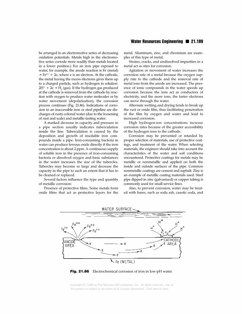
Water Resources Engineering n 21.109
be arranged in an electromotive series of decreasingoxidation potentials. Metals high in the electromo-tive series corrode more readily than metals locatedin a lower position.) For an iron pipe exposed towater, for example, the anode reaction is Fe (metal)→ Fe2+ + 2e, where e is an electron. At the cathode,the metal having the excess electrons gives them upto a charged particle, such as hydrogen in solution:2H+ + 2e → H2 (gas). If the hydrogen gas producedat the cathode is removed from the cathode by reac-tion with oxygen to produce water molecules or bywater movement (depolarization), the corrosionprocess continues (Fig. 21.86). Indications of corro-sion in an inaccessible iron or steel pipeline are dis-charges of rusty-colored water (due to the looseningof rust and scale) and metallic-tasting water.
A marked decrease in capacity and pressure ina pipe section usually indicates tuberculationinside the line. Tuberculation is caused by thedeposition and growth of insoluble iron com-pounds inside a pipe. Iron-consuming bacteria inwater can produce ferrous oxide directly if the ironconcentration is about 2 ppm. A continuous supplyof soluble iron in the presence of iron-consumingbacteria or dissolved oxygen and basic substancesin the water increases the size of the tubercles.Tubercles may become so large and decrease thecapacity in the pipe to such an extent that it has tobe cleaned or replaced.
Several factors influence the type and quantityof metallic corrosion:
Presence of protective films. Some metals formoxide films that act as protective layers for the
Fig. 21.86 Electrochemical cor
Copyright (C) 1999 by The McGraw-Hill Cothis product is subject to the terms of its Lic
metal. Aluminum, zinc, and chromium are exam-ples of this type of metal.
Strains, cracks, and undissolved impurities in ametal act as sites for corrosion.
Agitation or movement of water increases thecorrosion rate of a metal because the oxygen sup-ply rate to the cathode and the removal rate ofmetal ions from the anode are increased. The pres-ence of ionic compounds in the water speeds upcorrosion because the ions act as conductors ofelectricity, and the more ions, the faster electronscan move through the water.
Alternate wetting and drying tends to break upthe rust or oxide film, thus facilitating penetrationof the film by oxygen and water and lead toincreased corrosion.
High hydrogen-ion concentrations increasecorrosion rates because of the greater accessibilityof the hydrogen ions to the cathode.
Corrosion may be prevented or retarded byproper selection of materials, use of protective coat-ings, and treatment of the water. When selectingmaterials, the engineer should take into account thecharacteristics of the water and soil conditionsencountered. Protective coatings for metals may bemetallic or nonmetallic and applied on both theinside and outside surfaces of the pipe. Commonnonmetallic coatings are cement and asphalt. Zinc isan example of metallic coating materials used. Steelpipe dipped in zinc (galvanized) or copper tubing iscommonly used for small service lines.
Also, to prevent corrosion, water may be treat-ed with bases, such as soda ash, caustic soda, and
rosion of iron in low-pH water.
mpanies, Inc. All rights reserved. Use ofense Agreement. Click here to view.

21.110 n Section Twenty-One
lime, to reduce hydrogen-ion concentration and toinduce precipitation of thin films of carbonates,hydroxides, oxides, and so on on the walls of thepipes. These thin films reduce the ability of waterto corrode otherwise unprotected metal surfaces.Corrosion, however, normally precedes depositionof scale because iron must be in solution to reactwith the basic substances and dissolved oxygen inthe water to form scale.
Electrochemical corrosion of external surfaces ofpipelines and water tanks can be retarded by appli-cation of a direct current to the metal to be protectedand to another metal that acts as a sacrificial anode(Fig. 21.87). The potential applied to or produced bythe two metal surfaces must be large enough tomake the protected metal act as a cathode. The sacri-ficial anode corrodes and must be replaced periodi-cally. Zinc, magnesium, graphite, and aluminumalloys are commonly used for anode materials.
(American Water Works Association, “WaterQuality and Treatment,” 4th ed., McGraw-Hill,Inc., New York.)
21.56 Centrifugal PumpsThe purpose of any pump is to transform mechan-ical or electrical energy into pressure energy. Thecentrifugal pump, the most common waterworkspump, accomplishes that in two steps. The firsttransforms the mechanical or electrical energy intokinetic energy with a spinning element, or impeller.The kinetic energy is then converted to pressureenergy by diffuser vanes or a gradually divergingdischarge tube, called a volute (Fig. 21.88).
Water enters at the center, or eye, of theimpeller and is forced outward toward the casing
Fig. 21.87 Cathodic protection of a metal.
Copyright (C) 1999 by The McGraw-Hill Comthis product is subject to the terms of its Lic
by centrifugal force. The discharge head of a cen-trifugal pump is a function of the impeller diame-ter and speed of rotation.
Design factors requiring consideration in theselection of a centrifugal pump are net positivesuction head required, efficiency, horsepower, andthe head-discharge relationship.
Net positive suction head (NPSH) is the ener-gy in the liquid at the center line of the pump. Tohave practical meaning, it must be referred to aseither the required or available NPSH. RequiredNPSH is a characteristic of the pump and is givenby the manufacturer. Available NPSH is a charac-teristic of the system and is determined by theengineer. It is the pressure in the liquid over andabove its vapor pressure at the suction flange ofthe pump and is given, in feet, by
(21.147)
where pa = pressure, psia, on free-water surfaceor at center line of closed conduit
pν = vapor pressure, psia, of water at itspumping temperature
hf = friction loss in suction line, ft ofwater
z = elevation difference, ft, betweenpump center line and water surface
w = unit weight of liquid, lb/ft3
If the suction water surface is below the pump cen-ter line, z is negative. To prevent cavitation, it is nec-essary to have the available NPSH always greater
Fig. 21.88 Volute-type centrifugal pump.
panies, Inc. All rights reserved. Use ofense Agreement. Click here to view.
Water Resources Engineering n 21.111
than the required NPSH. For that reason, it is cus-tomary to analyze a required NPSH vs. dischargecurve with the brake horsepower, head, and effi-ciency curves when selecting a pump.
The operating point of a centrifugal pump isdetermined by the intersection of the pump’s head-capacity curve and the system head curve, as shownin Fig. 21.89. (Also included in Fig. 21.89 are theother curves used in pump selection.) A systemhead curve is a plot of the head losses in the systemvs. pump discharge. This curve shows the head dif-ferential that must be supplied by the pump. In atypical water-system analysis, there may be three orfour pertinent system head curves correspondingto various consumption rates. The intersection ofthese curves with the head vs. Q curve define arange of operation rather than a single point.
Selection of a centrifugal pump is largely a mat-ter of matching one of the many pumps availableto the system characteristics. An important consid-eration is that the point of maximum efficiency
Fig. 21.89 Curves used in se
Copyright (C) 1999 by The McGraw-Hill Cothis product is subject to the terms of its Lic
should be at or near the operating point. Centrifu-gal pumps are available in almost any capacitydesired, with lifts of up to 700 ft per stage. Efficien-cies may be as high as 93% for large pumps.
See also Art. 21.57 and check valves in Art. 21.58.(I. J. Karassik et al., “Pump Handbook,” 2nd ed.,
McGraw-Hill Book Company, New York.)
21.57 Well PumpsThese are classified as centrifugal, propeller, jet,helical, rotary, reciprocating, and air lift. Althoughcentrifugal pumps (Art. 21.56) are the most com-mon for both shallow-well and deep-well pumps,circumstances may dictate one of the other types.
Centrifugal pumps are used in wells over 6 in indiameter. They have capacities up to 4000 or 5000gal/min and heads up to 1200 ft, depending on thenumber of stages. Efficiencies may be as high as90% for the larger capacities; however, below 200gal/min, the maximum efficiency is 75 to 80%.
lection of a centrifugal pump.
mpanies, Inc. All rights reserved. Use ofense Agreement. Click here to view.

21.112 n Section Twenty-One
Propeller pumps are an axial-flow type. Theyare used in high-capacity low-head applications.
Jet pumps (Fig. 21.90) operate by dischargingwater through a nozzle and diverging conical tube,which are located at the well bottom. The diverg-ing conical tube creates lift by converting the high-velocity head to pressure head. The suction con-nection is made between the nozzle and entranceto the diverging tube. Jet pumps have low efficien-cies. They are used in small-capacity low-lift appli-cations, especially where the water contains sandor other impurities.
Helical pumps are a positive-displacementtype with a metal helical rotor rotating inside a
Fig. 21.90 Section through a jet pump (simpli-fied).
Copyright (C) 1999 by The McGraw-Hill Comthis product is subject to the terms of its Lic
rubber helical stator. The screw action of the rotorforces water through the pump and up the dis-charge pipe. Helical pumps are small-capacityhigh-lift pumps. They may be used in wells over 4in in inside diameter.
Rotary pumps are also of the displacementtype. They have a fixed chamber in which gears,vanes, cams, or pistons rotate with very close tol-erances. These pumps have relatively constantpartial-load efficiencies. Full-load efficiencies rangefrom 50 to 85%. Because of the close tolerances,they can be used only for sediment-free water.
Reciprocating pumps, either hand- or motor-driven, utilize piston action to move water. Theirpresent-day use is primarily for small-capacitylow-lift private applications.
Air-lift pumps generate lift by using air bubblesto decrease the specific weight of the column ofwater in the discharge pipe below that of the sur-rounding water in the well and create a pressure dif-ferential that forces the water out of the well. Air-liftpumps are the simplest and most foolproof of wellpumps since they have no submerged moving parts.They can be used in any well but have the disad-vantage of efficiencies below 50%.
Specific speed Ns is a widely used criterion forpump selection. It is the impeller speed corre-sponding to a discharge of 1 gal/min at 1 ft of headfor the most efficient design.
(21.148)
where n = impeller speed, r/min
Q = discharge, gal/min
H = head, ft
The favorable design range of Ns for radial-flow(centrifugal) pumps is from 1500 to 4100. For Nsbetween 4100 and 7500, mixed-flow pumps havingboth radial and axial characteristics should beused, and for Ns above 7500, axial-flow (propeller)pumps should be used.
Shallow-well pumps have their motors andimpellers at ground level, so that the entire lift issuction. Since excessive suction lifts cause cavita-tion, the lift is limited by atmospheric pressure andthe velocity head at the impeller, which is a func-tion of specific speed. At sea level, the maximumpractical lift for a shallow-well pump is about 25 ft.
Deep-well pumps have their impellers closeenough to the water surface to eliminate cavita-
panies, Inc. All rights reserved. Use ofense Agreement. Click here to view.
Water Resources Engineering n 21.113
tion. The motor may be at ground level with a longshaft connecting it to the impellers, or it may be atthe bottom of the well, below and directly adjacentto the impellers. The former type is called a deep-well turbine pump and the latter a submersible pump.Deep-well turbine pumps can be used only forstraight wells. The pump shaft is supported atintervals of about 10 ft by rubber or metal bearings,which are water- or oil-lubricated, respectively. Ifsand is carried out with the water, an enclosed-shaft or submersible pump must be used to pre-vent bearing damage. Submersible pumps may beused in crooked wells. Other advantages includeease of increasing the well depth or lift and silentoperation. One disadvantage is that the motors aredifficult to reach for repairs.
(I. J. Karassik et al., “Pump Handbook,” 2nd ed.,McGraw-Hill Book Company, New York.)
21.58 ValvesWater facilities use many different types of valves.These are generally classified according to thefunction they perform. The two major water-valveclassifications are isolating and controlling.
Isolating valves are used for separating or shut-ting off sections of pipe, pumps, and controldevices from the rest of the system for inspectionand repair purposes. The major types of isolatingvalves are gate, plug, sluice gate, and butterfly.
A control valve is normally used for continu-ously controlling pressures and flow rates. Check,needle, globe, air-relief, pressure-regulating, pres-sure-relief, and altitude valves are usually consid-ered as control valves.
Gate valves are the isolating valves used mostoften in distribution systems, primarily because oftheir low cost, availability, and low head loss whenfully open. They have limited value as control orthrottling devices because of seat wear and thedownstream deflection and chatter of the gate disk.Also, the open area and rate of flow through thevalve are not proportional to the percentage open-ing of the valve when partly open. Corrosion, solidsdeposition, tubercle formation, large pressure dif-ferences, and thermal expansion produce difficul-ties in opening normally closed gate valves or inclosing normally open gate valves. Periodic inspec-tion and operation of valves that are infrequentlyoperated will prevent many operational difficulties.Some of the larger gate valves have gear-reduction
Copyright (C) 1999 by The McGraw-Hill Cothis product is subject to the terms of its Lic
drives to permit manual operation. Very largevalves are operated by hydraulic and electric power.
A plug valve may be used for both control andisolation purposes. It consists of a cylindricallyshaped plug (with a rectangular slot or circular ori-fice) placed in a close-fitting cylindrical seat perpen-dicular to the direction of flow. Cone and sphericalvalves are special types of plug valves. Plug, cone,and spherical valves can all be fully closed oropened by a 90° rotation of the plug. The valvesmay or may not be lubricated (large iron valves usu-ally are). Hydraulic or electric power is commonlyutilized for operating the larger valves. Small plugvalves are commonly used for isolation purposes ondomestic and commercial service connections andare known as service, curb, or corporation cocks.Usually, because the meter is not directly adjacent tothe distribution pipe, three valves must be used, oneat the service connection, one just upstream of themeter, and one between the meter and the cus-tomer’s service line. Plug and cone valves are alsoused for throttling and remote-control shutoff. Lowhead loss, in-service lubrication features, and easy,fast operation, even in the presence of unequalpressures across the valve, are the major advantagesof plug-type valves. But these valves cost more thangate, globe, and butterfly valves.
Butterfly valves can be used for throttling andisolation purposes. The butterfly-valve mechanismconsists of a relatively thin circular disk pivoted ona horizontal shaft. Hand or motor power, appliedthrough a gear-reduction device, rotates the disk.Simplicity of construction and quick, easy opera-tion are reasons why these valves are replacingsluice gates and gate valves in many locations. LosAngeles has replaced many sluice gates in reser-voir towers with butterfly valves having seats ofcorrosion-resistant metal, rubber, or Neoprene. Adisadvantage of butterfly valves is the higher costrelative to sluice gates or gate valves.
Sluice gates are mainly used on the sides ofreservoir control towers and in open-channelstructures where pressure on one side of the gatehelps to seat it and prevent water leakage. Diffi-culties with leakage and corrosion of gate framesand stems are the main disadvantages of sluicegates. Low cost and ease of operation in open-channel flow conditions are the major advantages.
A needle valve is made of a streamlined plug orneedle that fits into a small orifice with a carefullymachined seat. Needle valves are used for accurate
mpanies, Inc. All rights reserved. Use ofense Agreement. Click here to view.
21.114 n Section Twenty-One
control of water flow because a large movement ofthe needle is necessary before any measurablechange of flow rate takes place. Needle valves arenot normally used for isolating purposes becauseof the high head losses produced by water flowthrough the small orifices. Large-sized needlevalves are used for flow regulation under highheads, such as for free discharge from reservoirs.Interior-differential, tube, and hollow-jet are threeof the most common types of large needle valves.
Globe valves are commonly used in smaller sizesfor domestic purposes. The valve mechanism con-sists of a screw-operated disk that is forced down ona circular seat. Because of high head losses, globevalves are rarely used for isolation purposes, butthey are commonly used for pressure regulation inwater-distribution systems. Many automatic controlvalves, such as pressure regulators and altitude,check, and relief valves, have globe-valve bodieswith various types of control mechanisms.
Pressure-regulating valves are used to reducepressures automatically. An air-relief and inlet valveserves the dual purpose of allowing air to eitherescape or enter a pipeline. Air that accumulates athigh points in a pipe impedes water flow and shouldbe allowed to escape through an air-relief valveplaced at this location. Furthermore, draining waterfrom low elevations in a pipeline may cause negativepressures at higher elevations and collapse a pipe.Air should be allowed to enter through air-relief andinlet valves at the high points to prevent this.
Pressure-relief valves are used to release excesspressure in an enclosure. Often, these excess pres-sures are caused by sudden closure of a valve.
Altitude valves are used to control the waterlevel of elevated reservoirs. A pressure-activatedcontrol closes the altitude valve when the tank is fulland opens the valve to allow water to flow from thetank when pressure below the valve decreases.
Check valves are used in pipelines to allow forone-directional flow only. Check valves placed incentrifugal-pump suction lines are called footvalves. These valves hold water in the suction lineand pump case so that the pump will not needmanual priming when started. The most commoncheck valve is the swing type.
21.59 Fire HydrantsA fire hydrant normally consists of a cast-iron bar-rel and a gate or compression-type shutoff valve,
Copyright (C) 1999 by The McGraw-Hill Comthis product is subject to the terms of its Lic
which connects the barrel to the main. Two or morehose outlets are normally located in the barrelabove the ground surface. Usually, an additionalgate valve is required between the hydrant and themain to allow for shutoff and repair of the hydrant.
The number of 21/2-in-diameter hose outlets on ahydrant determines its class. For example, a hydrantwith two hose outlets is called a two-way hydrant.
Fire-hydrant construction standards have beenestablished by the American Water Works Associa-tion and the American Insurance Association.These standards relate the diameter of the barrel tothe size of the main-valve opening. A barrel diame-ter of at least 4 in is required for a two-way hydrant,5 in for a three-way hydrant, and 6 in for a four-way hydrant. A minimum of two hose outlets isrequired on a fire hydrant. Where pumper serviceis necessary for adequate water pressure, a largepumper outlet must be furnished. This may takethe place of one of the smaller 21/2-in hose outlets.The minimum allowable diameter for the pipe con-nection between the main and the hydrant is 6 in.
Fire hydrants usually are either dry or wet bar-rel, depending on the location of the main valve inthe hydrant. The main valve in the dry-barrel typeshould be located below the frost line. When thevalve is in a closed position, a drain should be opento prevent freezing of water in the barrel. The wet-barrel, or California type, hydrants have the mainvalve located near the hose outlets. Many firehydrants have a safety joint above the ground sur-face to permit removal of the upper part of the bar-rel with a minimum loss of water.
Hose connections 31/16 in in diameter with 71/2
threads per inch have been selected by the AmericanInsurance Association as standard to allow for inter-change of fire-fighting equipment between cities.
Friction losses should not exceed 21/2 psi in ahydrant and 5 psi between the main and outletwhen flow is 600 gal/min.
21.60 Metering DevicesMetering devices are classified as either velocity ordisplacement types. Velocity types measure thevelocity of flow either directly by current-measur-ing devices or indirectly by venturi-principledevices and are usually calibrated to indicate theflow rate directly. The velocity-type meteringdevices are applied to measurement of flows instreams, rivers, and large pipes, such as trunk lines
panies, Inc. All rights reserved. Use ofense Agreement. Click here to view.
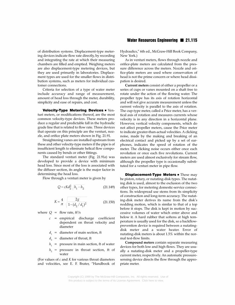
Water Resources Engineering n 21.115
of distribution systems. Displacement-type meter-ing devices indicate flow rate directly, by recordingand integrating the rate at which their measuringchambers are filled and emptied. Weighing metersare also displacement-type metering devices, butthey are used primarily in laboratories. Displace-ment types are used for the smaller flows in distri-bution systems, such as meters for individual cus-tomer connections.
Criteria for selection of a type of water meterinclude accuracy and range of measurement,amount of head loss through the meter, durability,simplicity and ease of repairs, and cost.
Velocity-Type Metering Devices n Ven-turi meters, or modifications thereof, are the mostcommon velocity-type devices. These meters pro-duce a regular and predictable fall in the hydraulicgrade line that is related to flow rate. Three devicesthat operate on this principle are the venturi, noz-zle, and orifice plate meters shown in Fig. 21.91.
Straightening vanes are installed upstream fromthese and other velocity-type meters if the pipe is ofinsufficient length to eliminate helical flow compo-nents caused by bends or other fittings.
The standard venturi meter (Fig. 21.91a) wasdeveloped to provide a device with minimumhead loss. Since most of the loss is associated withthe diffuser section, its angle is the major factor indetermining the head loss.
Flow through a venturi meter is given by
(21.149)
(21.150)
where Q = flow rate, ft3/s
c = empirical discharge coefficientdependent on throat velocity anddiameter
d1 = diameter of main section, ft
d2 = diameter of throat, ft
h1 = pressure in main section, ft of water
h2 = pressure in throat section, ft ofwater
(For values of c and K for various throat diametersand velocities, see E. F. Brater, “Handbook of
Copyright (C) 1999 by The McGraw-Hill Cothis product is subject to the terms of its Lic
Hydraulics,” 6th ed., McGraw-Hill Book Company,New York.)
As in venturi meters, flows through nozzle andorifice-plate meters are calculated from the pres-sure difference across the meters. Nozzle and ori-fice-plate meters are used where conservation ofhead is not the prime concern or where head dissi-pation is desired.
Current meters consist of either a propeller or aseries of cups or vanes mounted on a shaft free torotate under the action of the flowing water. Thepropeller type has its axis of rotation horizontaland will not give accurate measurement unless thecurrent velocity is parallel to the axis of rotation.The cup-type meter, called a Price meter, has a ver-tical axis of rotation and measures currents whosevelocity is in any direction in a horizontal plane.However, vertical velocity components, which donot affect propeller meters, cause the Price meterto indicate greater-than-actual velocities. A clickingnoise, made by the making and breaking of anelectrical contact and picked up by a set of ear-phones, indicates the speed of rotation of themeter. The clicking noise occurs either once eachrevolution or once each five revolutions. Currentmeters are used almost exclusively for stream flow,although the propeller type is occasionally substi-tuted for a venturi meter in pipe flow.
Displacement-Type Meters n These maybe piston, rotary, or nutating-disk types. The nutat-ing disk is used, almost to the exclusion of the twoother types, for metering domestic-service connec-tions. Its widespread use stems from its simplicityof construction and long-term accuracy. The nutat-ing-disk meter derives its name from the disk’snodding motion, which is similar to that of a topbefore it stops. The disk is kept in motion by suc-cessive volumes of water which enter above andbelow it. A hard rubber that softens at high tem-perature is usually used for the disk, so a backflow-prevention device is required between a nutating-disk meter and a water heater. Error ofnutating-disk meters is about 1.5% within the nor-mal test-flow limits.
Compound meters contain separate measuringdevices for both low and high flows. They are usu-ally a nutating-disk meter and a propeller-typecurrent meter, respectively. An automatic pressure-sensing device directs the flow through the appro-priate meter.
mpanies, Inc. All rights reserved. Use ofense Agreement. Click here to view.

21.116 n Section Twenty-One
Fig. 21.91 Venturi-type metering devices: (a) Standard venturi meter. (b) Nozzle meter. (c) Orifice-plate meter.
21.61 Water RatesThe interests of the public and individual customersof water-supply systems can best be served by self-sustained, utility-type enterprises. Rates charged tofinance these systems should be based on soundengineering and economic principles and designedto avoid discrimination between classes of cus-tomers. Gross revenue should cover operating andmaintenance expenses, fixed charges on capitalinvestment, and development of the system. Billingsfor water should be based on metered use and suchfixed charges as are required. Rate structures are typ-
Copyright (C) 1999 by The McGraw-Hill Comthis product is subject to the terms of its Lic
ically based on demand, load factors, fire use, peakrates of use, seasonal use, and similar items. The sys-tem of accounting should conform to the legallyestablished system of accounting prescribed for theutility, if any, or to some other recognized system.
Rates most commonly used today are flat rate,step rate, and block rate.
Flat rate is a monthly or quarterly charge thatdoes not vary with the amount of water used. Thistype of charge tends to encourage waste. Althoughit has been commonly employed in small commu-nities where water is not metered, flat rate is fallinginto disuse.
panies, Inc. All rights reserved. Use ofense Agreement. Click here to view.

Water Resources Engineering n 21.117
With step rate, customers are charged at one rateper 1000 gal for all water used. The rate a customerpays decreases as the total quantity used increases.The major objection to this method is that a cus-tomer who uses a quantity slightly less than thepoint of rate change will pay more than the cus-tomer who uses a little more.
The block rate schedule consists of one price per1000 gal for the first volume or block of water usedper billing period and lesser rates for additionalblocks. This type of pricing tends to discouragewaste but does not restrict usage unnecessarily.Both the step and block rates can have a monthlyservice charge.
When fixing a system of rates, the suppliershould consider the following factors: (1) cost ofcollection facilities, treatment chemicals, pumpingenergy, and, where applicable, buying water from awholesale supplier; (2) cost of distribution andtreatment facilities; and (3) cost, including meteringand billing, of serving an individual customer. Costcomponent 1, called the commodity component, isdirectly dependent on total usage and thereforeshould be distributed equally to all water sold. Costcomponent 2, called the demand component,depends on the peak usage of a customer. If a cus-tomer’s usage is zero during peak hour, it will notappreciably affect the cost or design of distributionfacilities. Since peak-hour demands usually governthe design of a distribution system, this is a goodcriterion for allocating distribution costs. It is gener-ally recognized that residential areas, where themajority of small users are, have very high ratios ofpeak demand to total usage and should thereforepay a major share of the demand component. Boththe step and block rates attempt to allocate this costto the small user by charging a higher rate for thefirst water sold to a customer and charging decreas-ing rates with increased usage. For most distribu-tion systems, a large share of the demand compo-nent also should be allocated to fire service. Theportion attributed to fire service is usually paid bytaxes. Cost component 3, called the customer com-ponent, is usually distributed to the customer by amonthly service charge that depends only on thesize of service. This charge is usually small.
Hydroelectric Power and DamsHydroelectric plants, which generate electricpower from water dropping a sufficient vertical
Copyright (C) 1999 by The McGraw-Hill Cothis product is subject to the terms of its Lic
distance to drive large hydraulic turbines, supplyan appreciable portion of the electric power con-sumed in the U. S. Hydroelectric generation is anattractive power source because it is a renewableresource and a nonconsumptive use of water. Atypical hydroelectric plant consists of a dam todivert or store water from a river or stream; canals,tunnels, penstocks, and a forebay to convey waterto turbines; draft tube, tunnel, or tailrace to returnwater downstream to the river or stream; turbinesand governors; generators and exciters; equipmentsuch as protective devices and regulators; a build-ing to house the machinery and equipment; andtransformers, switching equipment, and powertransmission lines to deliver the power producedto a load center for distribution to consumers.
21.62 Hydroelectric-PowerGeneration
Hydroelectric power is electrical power obtainedfrom conversion of potential and kinetic energy ofwater. The potential energy of a volume of water isthe product of its weight and the vertical distanceit can fall:
(21.151)
where PE = potential energy
W = total weight of the water
Z = vertical distance water can fall
Because the kinetic energy of the supply source isvery small or zero in most hydropower (hydroelec-tric power) developments, the kinetic-energy termdoes not appear in power formulas.
Power is the rate at which energy is producedor utilized.
1 horsepower (hp) = 550 ft⋅lb/s
1 kilowatt (kW) = 738 ft⋅lb/s
1 hp = 0.746 kW
1 kW = 1.341 hp
Power obtained from water flow may be computedfrom
(21.152a)
mpanies, Inc. All rights reserved. Use ofense Agreement. Click here to view.

21.118 n Section Twenty-One
(21.152b)
where kW = kilowatts
hp = horsepower
Q = flow rate, ft3/s
w = unit weight of water = 62.4 lb/ft3
h = effective head = total elevation dif-ference minus line losses due to fric-tion and turbulence, ft
η = efficiency of turbine and generator
Hydroplants can be classified on a basis ofreservoir capacity and use as run-of-river hydrowithout storage, base-load plants, run-of-riverplants with storage, and peak-load plants.
Run-of-River Hydro without Storage n
This type of plant has no storage facilities. Powergeneration is totally dependent on the flow of theriver. A development of this type is usually built forsome other purpose, such as navigation, powerproduction being only incidental.
The economics of a run-of-river hydroplantdepend on the minimum flow of the river. If theminimum flow is very low, it will be necessary toinvest money in steam-generation facilities to pro-vide supplemental power during low-flow peri-ods. Therefore, the value of the plant will be onlythe fuel saved that would otherwise be requiredfor steam generation.
Base-Load Hydro Plants n This type is alsoa run-of-river hydroplant without storage, but it islocated on a river that provides a minimum flowcapable of serving the power demand withoutsupplementary steam-generating facilities. Thereliable plant capacity is set below the expectedminimum flow in the river. This type of run-of-river hydroplant utilizes only a small proportion ofthe flow of a river. It must pass not only high sea-sonal flows but also the water it cannot utilize dur-ing hours of low power demand.
Cost of a base-load plant can be compared withthe cost of the steam capacity that would be neces-sary to serve power demands if hydrogenerationwere not developed.
Run-of-River Plants with Storage n Asmall amount of storage can greatly increase the
Copyright (C) 1999 by The McGraw-Hill Comthis product is subject to the terms of its Lic
reliable capacity of a hydroplant. The water notrequired for generation during hours of low powerdemand can be stored and used for generationduring periods of peak demand.
Storage can be provided for a daily, weekly, orseasonal cycle. On a daily cycle, the required reser-voir capacity is less than the river’s daily flow vol-ume. On a weekly cycle, the flow during the periodsof low power demand on weekends is also stored togive additional capacity for peak periods during theweek. On a seasonal cycle, the high flood flows arestored to be used during periods of low flow. Theseasonal operation requires many times the storagenecessary for weekly or daily operation and there-fore may be uneconomical unless the reservoir ismultipurpose. Then, part of its cost can be under-written by flood-control or irrigation projects.
Peak-Load Plants n The power demand onan electrical system fluctuates from a daily high toa nightly low. Depending on the size of the utilityand type of customers served, peak demands maybe several times the magnitude of the lowdemands encountered at night. These fluctuationsin demand necessitate generation facilities whosefull capacity is used only a few hours a day, duringperiods of peak power demand (Fig. 21.92).
Capacity factor is the percentage of the timethe full capacity of a plant is used or the ratio of theaverage power the plant produces to the plant’scapacity. It can be computed on a daily, weekly, oryearly basis.
Hydroplants that are used mainly to supplypower for the periods of peak demand are gener-ally called peak-load plants. The main classes ofpeak-load plants are pumped-storage plants andrun-of-river plants with storage.
If sufficient generating capacity and reservoirstorage are planned for a run-of-river hydroplant,only a relatively small supply of water is needed toproduce a high generation capacity for a few hoursduration. This enables a large utility to use steamgeneration at a high capacity factor where it ismost efficient and to supply peak demands fromhydroplants.
Pumped Storage n This is a means of storinglarge quantities of energy, generated during peri-ods when excess generating capacity is available, tobe used at some future time. Water is pumped froma low reservoir to a higher one by energy from
panies, Inc. All rights reserved. Use ofense Agreement. Click here to view.

Water Resources Engineering n 21.119
Fig. 21.92 Daily load curves for generating plants. (Department of Water and Power, Los Angeles, Calif.)
steam or base-load hydro when power demand islow. When needed, the water generates power byflowing through a turbine back into the low reser-voir. Because of friction loss in the penstock andlosses due to the imperfect efficiencies of pumpsand turbines, only two-thirds of the energyrequired to pump the water is recovered.
The balance of energy between pumping andgenerating can be on a daily or weekly basis. Butbecause the weekly cycle requires several timesmore reservoir storage than the daily cycle, it usu-ally is not as economical.
When pumped storage is operated at a highcapacity factor to transfer large quantities of elec-tric energy from off-peak to peak, the energy lossmay make it uneconomical. This undesirable ener-gy-loss feature of pumped storage is overcomewhen it is used as reserve capacity.
Electrical systems require what is called spin-ning reserve, which is capacity above that necessaryto serve the expected maximum load, readyinstantly to generate power in case of failure ofgenerating equipment or an unanticipated high
Copyright (C) 1999 by The McGraw-Hill Cothis product is subject to the terms of its Lic
power demand. Many utilities keep a spinningreserve capacity equal to the size of their largestsingle generating unit, or 15% of their maximumdemand (Fig. 21.92).
(V. J. Zipparo and H. Hasen, “Davis’ Handbookof Applied Hydraulics,” 4th ed., McGraw-Hill BookCompany, New York.)
21.63 DamsDams are usually classified on the basis of the typeof construction material or the method used toresist water pressure. The main classifications aregravity, arch, buttress, earth, and rock-fill.
Gravity dams are concrete or masonry damsthat resist the forces acting on them entirely bytheir weight. Figure 21.93 shows the forces that acton a typical gravity dam. The largest force is usual-ly the hydrostatic force of the water F1. Its distribu-tion is triangular, varying from zero at the top tofull hydrostatic at the bottom. Force F2 representssilt pressure, which results from deposition of siltat the base of the dam. This silt pressure can be cal-
mpanies, Inc. All rights reserved. Use ofense Agreement. Click here to view.

21.120 n Section Twenty-One
Fig. 21.93 Forces acting on a concrete gravity dam.
culated by Rankine’s theory for earth pressureusing the submerged weight of the silt.
Force F3 represents ice pressure against the faceof the dam. In cold climates, ice, which forms onthe reservoir surface, expands when the tempera-ture rises and exerts a force on the top of a dam. Inthe past, ice pressures as high as 50,000 psf havebeen used for the design of dams in the north;however, today it is realized these values are muchtoo high. A method of calculating these forces, pre-sented by Edwin Rose, gives values ranging from2000 to 10,000 psf, depending on the rate of tem-perature rise and restraining conditions at theedges of the reservoir. (E. Rose, “Thrust Exerted byExpanding Ice,” Proceedings of the American Societyof Civil Engineers, May 1946.)
Practically all regions in the United States aresubject to earthquakes of varying intensity. Earth-quakes cause vertical and horizontal accelerations ofthe earth, which create forces on any object restingon it. The magnitude of these forces equals the massof the object times the acceleration from the earth-quake. These accelerations occur in every direction,so the effect of the forces must be analyzed for alldirections. Most dams in seismically active regions in
Copyright (C) 1999 by The McGraw-Hill Comthis product is subject to the terms of its Lic
the United States have been designed for an acceler-ation equal to 0.1 g, where g is the acceleration dueto gravity. The effect of accelerations on the dam isrepresented in Fig. 21.93 by forces F4 and F5. Force F6represents the inertial force of the water on the faceof the dam. A close approximation of the force, givenby Eq. (21.153), was developed by von Karman.(“Pressure on Dams During Earthquakes,” discus-sion by von Karman, Transactions of the American Soci-ety of Civil Engineers, vol. 98, p. 434, 1933.)
(21.153)
where w = unit weight of water, lb/ft3
a = acceleration due to earthquake, ft/s2
h = depth of water behind dam, ft
The force F6 acts at a point 0.425h above the base.Force F7 is due to the weight of water on an
inclined face. Gravity dams usually have aninclined upstream face to facilitate construction.
Force F8 represents an uplift force that acts onthe undersurface of any section taken through thedam or under the base of the dam. This uplift iscaused by the seepage of water through pores or
panies, Inc. All rights reserved. Use ofense Agreement. Click here to view.

Water Resources Engineering n 21.121
imperfections in the foundations or through imper-fectly bonded construction joints in the masonry. Inthe past, engineers assumed that, because of bear-ing contact, this pressure acted only on some per-centage of the total area. Recent belief, however, isthat uplift acts on 100% of the area of the base.
A process used to reduce uplift pressures callsfor grouting along the heel and use of drainsbehind the grout. When the base is not drained,the uplift pressure is assumed to vary linearly frombetween full and one-half hydrostatic pressure atthe heel to the full tailwater pressure at the toe.
Force F9 represents the weight of the dam. Itacts at the centroid of the cross-sectional area ofthe dam.
Summation of the vertical forces and ofmoments about any point yields the foundationpressure. The foundation pressure at the heel ofthe dam should be compressive. Hence, the resul-tant of all forces acting on the dam should fallwithin the middle third of the base of the dam.
The basic modes of failure possible for a gravitydam are by sliding along a horizontal plane, over-turning by rotating about the toe, or failure of thefoundation material. The first two modes dependmainly on the cross-sectional shape of the dam,whereas the third depends on both the cross-sec-tional shape and the foundation material.
Gravity dams can be built on earth foundations,but their height in these cases has been limited toaround 65 ft. The main reason gravity dams are usedis that they can pass large flood flows over their crestwithout damage. Their first cost and maintenancecost are usually greater than those of earth or rock-fill dams of comparable height and crest length.
Arch dams are concrete dams that carry theforce of the water through arch action. Stresses inan arch dam may be determined with computersby the finite-element method or by an approxi-mate method in which the water force is dividedbetween elements: a series of horizontal archesthat span between the abutments and a series ofvertical cantilevers fixed at the foundation. Thedistribution of load between the arches and can-tilevers is determined by the trial-load method.First, a division of the load is assumed and thedeflections in the arches and cantilevers are com-puted. The deflection of an arch at any point mustequal the deflection of the cantilever at the samepoint. If the deflections are not equal, a new divi-sion of the load is assumed and the deflections
Copyright (C) 1999 by The McGraw-Hill Cothis product is subject to the terms of its Lic
recalculated. This process is continued until equaldeflections are obtained.
The external forces an arch dam must resist arebasically the same as those on a gravity dam; how-ever, their relative importance is much different.On arch dams, uplift is not so important, but iceloads and temperature stress are much more criti-cal. Arch dams require much less concrete thangravity dams and usually have a much lower firstcost. They are not suited to most sites, however,since they must be located in a relatively narrowcanyon supported by good rock abutments.
Buttress dams consist of a watertight membranesupported by a series of buttresses at right angles tothe axis of the dam. Although there are many typesof buttress dams, those widely used are the flat-slaband the multiple-arch. These differ in that the water-supporting membrane for the flat-slab type is a con-tinuous concrete slab spanning the buttresses. In themultiple-arch, the membrane is a series of concretearches. The multiple-arch requires less reinforcingsteel and can span longer distances between but-tresses, but its formwork is more expensive.
The upstream face of a buttress dam is usuallyinclined at about 45°. The weight of the water onthe face is necessary to increase the dam’s resis-tance to sliding and overturning.
The forces acting on a buttress dam are exactlythe same as those that act on a gravity dam. How-ever, the vertical load of the water is much greateron a buttress dam, and uplift forces are smaller.The modes of failure are also the same, but thestructural design is much more critical.
Although buttress dams usually require lessthan half the volume of concrete required by grav-ity dams, they are not necessarily less expensivebecause of the large amount of formwork and rein-forcing steel required. With the rapidly increasingcost of labor over the past several decades, the but-tress dam has lost much of its earlier popularity.
Earth dams are designed to utilize materialsavailable at the dam site. They can be constructedof almost any material with very primitive con-struction equipment. Successful earth dams havebeen built of gravel, sand, silt, rock flour, and clay.If a large quantity of pervious material, such assand and gravel, is available and clayey materialsmust be imported, the dam would have a smallimpervious clay core, the material available locallymaking up the bulk of the dam. Concrete has beenused for an impervious core, but it does not pro-
mpanies, Inc. All rights reserved. Use ofense Agreement. Click here to view.
21.122 n Section Twenty-One
vide the flexibility of clay materials. If perviousmaterial is not available, the dam can be construct-ed of clayey materials with underdrains of import-ed sand or gravel under the downstream toe to col-lect seepage and relieve pore pressures.
Slopes of an earth dam are rarely greater than 2horizontal to 1 vertical and are usually about 3 to 1.The governing criterion is usually the stability ofthe slopes against slide-out failure. Stability underthe action of seismic forces is especially critical. Forsoils in which pore pressure changes develop as aresult of shear strain induced by an earthquake,determination of appropriate values for yieldacceleration is very difficult. For some types of soil,no well-defined yield acceleration exists; displace-ments occur over a wide range of accelerations.
Another factor that sometimes determines thesteepness of the slopes is the amount of seepagethat can be tolerated. If the dam is on a perviousfoundation, it may be necessary to increase thebase width to reduce seepage. The seepage mayalso be reduced by placing an impervious blanketon the upstream side of the dam to increase theseepage path or by using a cutoff wall in the foun-dation, such as sheetpiling or a clay-filled trench.
Earth dams can be built to almost any heightand on foundations not strong enough for con-crete dams. Improvements in earth-moving equip-ment have resulted in a decreased cost for earthdams, and rising labor costs have increased thecost for concrete dams.
Rock-fill dams usually consist of a dumped rockfill, a rubble cushion of laid-up stone on the upstreamface, bonding into the dumped rock, and anupstream impervious facing, bearing on the rubblecushion, with a cutoff wall extending into the foun-dation. The dumped rock fill may consist of rocksvarying in size from small fragments to bouldersweighing as much as 25 tons. The fill is usually com-pacted by dropping the rock, sometimes from as highas 175 ft. onto the fill. Sluicing of the fill with high-pressure hoses is also used to wash fines frombetween contact points of the rock and reduce settle-ment. The rubble cushion consists of rocks individu-ally placed to reduce the voids and provide supportfor the impervious facing. The facing is usually con-crete, or wood over concrete, although steel has beenused occasionally. The cutoff wall is usually concrete.
Rock-fill dams are generally designed empiri-cally. Low rock-fill dams may have an upstreamface as steep as 1/2 horizontal on 1 vertical. The
Copyright (C) 1999 by The McGraw-Hill Comthis product is subject to the terms of its Lic
downstream face is usually 1.3 on 1, the naturalangle of repose of rock. For dams over 200 ft high,both the upstream and downstream faces are usu-ally on a slope of 1.3 on 1.
The major problem encountered in rock-fill damsis large settlements that occur after construction whenthe reservoir is first filled. Vertical settlements andhorizontal displacements in excess of 5% of the heightof the dam have occurred; therefore, the imperviousfacing must be very flexible or damage will occur dur-ing settlement. One solution to this problem has beento put a temporary facing on the dam and to replaceit with a permanent facing after settlement has takenplace. Temporary facings are usually of wood.
Rock-fill dams are used extensively in remotelocations where cement is expensive and the mate-rials for an earth dam are not available. Their costcompares favorably with that of concrete dams.Leakage should be expected, but rock-fill dams arevery stable and have been overtopped withoutsuffering major damage.
(V. J. Zipparo and H. Hasen, “Davis’ Handbookof Applied Hydraulics,” 4th ed., McGraw-Hill BookCompany, New York; “Design of Small Dams” and“Embankment Dams,” U. S. Bureau of Relamation;“Earth and Rockfill Dams: General Design andConstruction Considerations,” EM 1110-2-2300, U.S. Army Corps of Engineers.)
21.64 Hydraulic TurbinesIn the past, hydraulic power-generating machinesmeant a large number of different types of equip-ment. Today, however, the turbine is the only typeof importance in hydraulic power generation. Itsfunction is transformation of the kinetic andpotential energy of water into useful work.
Turbines are classified as impulse turbines andreaction turbines.
Impulse turbines utilize the energy of waterby first transforming it into kinetic energy, by freedischarge of the water through a nozzle. The noz-zle is directed at buckets positioned along theperimeter of a water wheel. The force of the waterstriking these buckets causes the wheel to rotate,providing power.
The only type of water wheel used today inimpulse turbines was developed in 1880 by Pelton—the Pelton wheel (Fig. 21.94). The wheel is coveredby a housing to prevent splashing and to guide thedischarge after the water strikes the wheel.
panies, Inc. All rights reserved. Use ofense Agreement. Click here to view.

Water Resources Engineering n 21.123
In most impulse turbines, the water wheelrotates on a horizontal shaft and is acted on by thedischarge from one or two nozzles. But verticalshafts may be used with as many as six nozzles, toobtain a high efficiency for very low loads. In suchinstallations, efficiencies of 92% for full load andslightly below 90% for loads as low as one-quarterof full load have been obtained.
Impulse turbines are commonly used for headsgreater than 1000 ft. (An impulse turbine at the Reis-seck Power Plant in Austria operates under a neteffective head of 5800 ft.) There is no lower limit ofhead for impulse turbines. They have been used forheads as low as 50 ft; however, the reaction turbineis usually better suited to low heads at large flows.
Reaction Turbines n Types of reaction tur-bines include the Francis (Fig. 21.95a), the pro-peller-type (Fig. 21.95b) and the axial flow (Fig.21.95c). In these, the flow from the headwater tothe tailwater is in a closed conduit system.
The Francis turbine usually consists of fouressential parts: scroll case, wicket gates, runner,and draft tube.
The scroll case transfers the water from the pen-stock (supply pipe) to the wicket gates and runner. Itdistributes the water so that all points on the perime-ter of the runner receive the same quantity of water.
The wicket gates, located just outside theperimeter of the runner, control the amount ofwater that enters the turbine. When the powerdemand on the turbine changes, a governor actu-ates a mechanism that opens or closes the gates.
The runner is the part of the turbine that trans-forms the pressure and kinetic energy of the waterinto useful work. As the water flows through the tur-
Fig. 21.94 Impulse (Pelton) type of hydraulicturbine.
Copyright (C) 1999 by The McGraw-Hill Cothis product is subject to the terms of its Lic
bine, it changes direction. This creates a force on therunner, causing it to rotate and turn the generator.
The draft tube is a conical tube with divergingsides. It decelerates the flow discharged from therunner, so that the remaining kinetic energy maybe regained by conversion into suction head.
Francis turbines have a maximum efficiency ofabout 94% when operated at or close to full load.However, if the load drops below 50%, their effi-ciency decreases rapidly. Francis turbines are com-monly used for heads between 100 and 1000 ft. Atheads above 1000 ft. problems are encountered incontrolling cavitation and in building a scroll caseto take the high pressures. At heads below 100 ft.the propeller-type turbine is usually more efficient.
Propeller Turbines n There are two types ofpropeller turbines: the movable-blade type, such asthe Kaplan turbine, and the fixed-blade type. Theonly difference between the two is that the pitch ofthe propeller blades is adjustable in a Kaplan turbine.
The propeller turbine (Fig. 21.95) has the samebasic parts as the Francis turbine: scroll case, wick-et gates, runner, and draft tube. The basic differ-ence between the Francis turbine and the propellerturbine is in the shape of the runner. The runner ofa propeller-type turbine operates in the same man-ner as a fan or a ship’s propeller: The water mov-ing past the blades creates a force that causes therunner to rotate.
Propeller-type turbines are used for headsranging from a few feet to about 100 ft. The Kaplanturbine has an efficiency of about 94% for full loadand drops only to 92% for 40% load. The fixed-blade-type turbine also has an efficiency of about94% for full load; however, its efficiency drops offrapidly below full load.
Axial-Flow Turbines n These provideenhanced performance for operation under low-head and large capacity.
(V. J. Zipparo and H. Hasen, “Davis’ Handbookof Applied Hydraulics,” 4th ed., McGraw-Hill BookCompany, New York.)
21.65 Methods for Control ofFlows from Reservoirs
Any reservoir with an appreciable drainage areamust have a spillway to discharge flood flows with-
mpanies, Inc. All rights reserved. Use ofense Agreement. Click here to view.
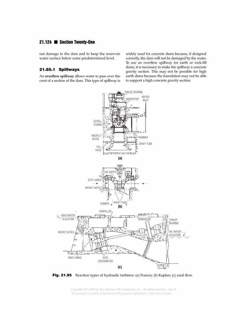
21.124 n Section Twenty-One
out damage to the dam and to keep the reservoirwater surface below some predetermined level.
21.65.1 Spillways
An overflow spillway allows water to pass over thecrest of a section of the dam. This type of spillway is
Fig. 21.95 Reaction types of hydraulic tu
Copyright (C) 1999 by The McGraw-Hill Cothis product is subject to the terms of its L
widely used for concrete dams because, if designedcorrectly, the dam will not be damaged by the water.To use an overflow spillway for earth or rock-filldams, it is necessary to make the spillway a concretegravity section. This may not be possible for highearth dams because the foundation may not be ableto support a high concrete gravity section.
rbines: (a) Francis; (b) Kaplan; (c) axial flow.
mpanies, Inc. All rights reserved. Use oficense Agreement. Click here to view.

Water Resources Engineering n 21.125
The discharge over an overflow spillway isgiven by the equation for discharge over a weir(Art. 21.34). Since the discharge varies as the headto the 3/2 power, overflow spillways keep the waterlevel within close limits even when there is a largevariation in flows.
It is desirable for an overflow spillway to havethe form of the underside of the nappe of a sharp-crested weir. This type of spillway, called an ogee
spillway, should be designed—as should all spill-ways—so that separation of the water from theface of the spillway will not occur. Thus, the dan-ger of cavitation will be eliminated.
In a chute spillway, water flows over a crestinto a steeply sloping, lined, open channel. Theflow is made supercritical to keep the size andlength of the chute to a minimum. Gradual verticalcurves should be used in the chute to avoid sepa-ration of the flow from the channel bottom.
Chute spillways are commonly used for earthand rock-fill dams where the topography allows achute to carry the water away from the toe to elim-inate the danger of undermining. The dischargeover the crest is given by the equations for dischargeover a weir or the entrance to an open channel.
In a side-channel spillway, the flow passesover a crest into a channel parallel to this crest. Thecrest is usually a concrete gravity section, althoughit can be concrete laid on the natural embankment.Side-channel spillways are often used in narrowcanyons where it is not possible to obtain sufficientcrest length for overflow or chute spillways. Theflow in the channel parallel to the crest is deter-mined by applying the momentum principle in thedirection of flow and assuming the energy of thewater flowing over the crest is completely dissipat-ed (U.S. Bureau of Reclamation, “Design of SmallDams,” Government Printing Office, Washington,DC 20402).
In a shaft spillway, sometimes called a morn-
ing-glory spillway, the water flows over a circularweir into a vertical shaft. The shaft terminates in ahorizontal conduit that carries the water past thedam. The weir can be sharp-crested, flared, orogee in cross section. (This type of spillway shouldnot be constructed over or through earth dams.) Ifthe topography is not suitable for a chute or side-channel spillway, a shaft spillway may be the bestalternative.
There are two conditions of discharge for ashaft spillway, both depending on the head on the
Copyright (C) 1999 by The McGraw-Hill Cothis product is subject to the terms of its Lic
weir. When the head is relatively low, the dis-charge is governed by the flow over the weir,which is directly proportional to the 3/2 power ofthe head on the weir. As the head increases, atsome point the discharge will no longer be con-trolled by the amount of water that can flow overthe weir but by the amount of water that can flowthrough the conduit. The discharge for this condi-tion is directly proportional to the 1/2 power of theelevation difference between the reservoir waterlevel and the level of discharge of the spillway con-duit. Once this second condition is reached, a largeincrease in head will cause only a small increase inflow. Since analytical analysis of discharge doesnot give good results on this type of spillway,model tests are usually employed.
A siphon spillway (Fig. 21.96) is a closed conduitfor discharging water over or through a dam. Theentrance to a siphon spillway is usually submergedbelow the normal water level so that it will not clogwith debris or ice. The discharge end of the siphonis usually sealed by deflecting the flow across thebarrel or by submerging it so that air cannot enter.
The air vent shown in Fig. 21.96 determines thereservoir level at which the siphon flow begins.When the reservoir water level rises above the vent,the siphon’s intake is sealed. Water flowing over thecrest of the siphon removes the air in the siphon andfull flow begins. Because the flow depends on thesiphoning action, siphon spillways hold the water
Fig. 21.96 Siphon spillway.
mpanies, Inc. All rights reserved. Use ofense Agreement. Click here to view.
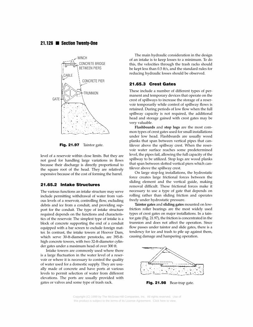
21.126 n Section Twenty-One
level of a reservoir within close limits. But they arenot good for handling large variations in flowsbecause their discharge is directly proportional tothe square root of the head. They are relativelyexpensive because of the cost of forming the barrel.
21.65.2 Intake Structures
The various functions an intake structure may serveinclude permitting withdrawal of water from vari-ous levels of a reservoir, controlling flow, excludingdebris and ice from a conduit, and providing sup-port for the conduit. The type of intake structurerequired depends on the functions and characteris-tics of the reservoir. The simplest type of intake is ablock of concrete supporting the end of a conduitequipped with a bar screen to exclude foreign mat-ter. In contrast, the intake towers at Hoover Dam,which serve 30-ft-diameter penstocks, are 395-ft-high concrete towers, with two 32-ft-diameter cylin-der gates under a maximum head of over 300 ft.
Intake towers are commonly used where thereis a large fluctuation in the water level of a reser-voir or where it is necessary to control the qualityof water used for a domestic supply. They are usu-ally made of concrete and have ports at variouslevels to permit selection of water from differentelevations. The ports are usually provided withgates or valves and some type of trash rack.
Fig. 21.97 Taintor gate.
Copyright (C) 1999 by The McGraw-Hill Comthis product is subject to the terms of its Lic
The main hydraulic consideration in the designof an intake is to keep losses to a minimum. To dothis, the velocities through the trash racks shouldbe kept less than 0.5 ft/s, and the standard rules forreducing hydraulic losses should be observed.
21.65.3 Crest Gates
These include a number of different types of per-manent and temporary devices that operate on thecrest of spillways to increase the storage of a reser-voir temporarily while control of spillway flows isretained. During periods of low flow when the fullspillway capacity is not required, the additionalhead and storage gained with crest gates may bevery valuable.
Flashboards and stop logs are the most com-mon types of crest gates used for small installationsunder low head. Flashboards are usually woodplanks that span between vertical pipes that can-tilever above the spillway crest. When the reser-voir water surface reaches some predeterminedlevel, the pipes fail, allowing the full capacity of thespillway to be utilized. Stop logs are wood planksthat span between slotted vertical piers which can-tilever above the spillway crest.
On large stop-log installations, the hydrostaticforce creates large frictional forces between thesliding element and the vertical guide, makingremoval difficult. These frictional forces make itnecessary to use a type of gate that depends onrolling rather than sliding friction and operatesfreely under hydrostatic pressure.
Taintor gates and sliding gates mounted on low-friction roller bearings are the most widely usedtypes of crest gates on major installations. In a tain-tor gate (Fig. 21.97), the friction is concentrated in thetrunnion and does not affect the operation. Sinceflow passes under taintor and slide gates, there is atendency for ice and trash to pile up against them,causing damage and hampering operation.
Fig. 21.98 Bear-trap gate.
panies, Inc. All rights reserved. Use ofense Agreement. Click here to view.

Water Resources Engineering n 21.127
Fig. 21.99 Drum gate.
Copyright (C) 1999 by The McGraw-Hill Cothis product is subject to the terms of its Lic
Bear-trap and drum gates allow the flow topass over the top. The bear-trap gate consists oftwo leaves hinged, as shown in Fig. 21.98. To raisea bear-trap gate, water is admitted to the spaceunder the leaves to force the leaves up. The drumgate (Fig. 21.99) consists of a segment of a cylinderthat is lowered into a recess in the crest when notin use. Because of the large recess required in thedam, drum gates are not suited to small dams.
(V. J. Zipparo and H. Hasen, “Davis’ Handbook ofApplied Hydraulics,” 4th ed., and H. E. Babbitt, J. J.Doland, and J. L. Cleasby, “Water Supply Engineer-ing,” McGraw-Hill Book Company, New York.)
mpanies, Inc. All rights reserved. Use ofense Agreement. Click here to view.

Copyright (C) 1999 by The McGraw-Hill Companies, Inc. All rights reserved. Use ofthis product is subject to the terms of its License Agreement. Click here to view.
blank page 21.128


![[ CIVIL ENGINEERING ] WATER RESOURCES ENGINEERING€¦ · 5th Semester B.TECH. [ CIVIL ENGINEERING ] WATER RESOURCES ENGINEERING The Need… water is curative in indigestion, water](https://static.fdocuments.in/doc/165x107/5e95b6ba269fea172b4b7b4e/-civil-engineering-water-resources-engineering-5th-semester-btech-civil-engineering.jpg)