21

A nonlinear difference equation

In general a nonlinear difference equation

xn+1 = f(xn) (21.1)

can have very complicated behaviour. In this chapter we will look at a

particular example,

xn+1 = rxn(1 − xn),

where r is a parameter that we will vary between 0 and 4.

In order to describe the solution we will use qualitative ideas similar those

we used to study autonomous equations (x = f(x)) in chapter 7, and con-

centrate on what happens to solutions ‘eventually’.

When we have a difference equation the solution is given by a sequence

of iterates of f ,

x0, x1 = f(x0), x2 = f(f(x0)), x3 = f(f(f(x0))), . . .

Since these nested fs rapidly become unmanageable we adopt the notation

fn(x) to mean f applied n times to x,

fn(x) = f(f(f(· · · f︸ ︷︷ ︸

n times

(x) · · ·)).

We can write the ‘solution’ of (21.1) that has x0 = y0 as xn = fn(y0), but

this is clearly no more descriptive of the solution than (21.1) itself.

21.1 Fixed points and stability

In order to describe the dynamics of solutions we make use of similar con-

cepts as we used for the 1d dynamical systems that arise from autonomous

130

21.1 Fixed points and stability 131

differential equations. For an iterated map like (21.1) a stationary point is

a point x∗ such that

f(x∗) = x∗,

so that if xn = x∗ then xn+1 = x∗. [This corresponds to the ‘stationary

points’ of x = f(x).]

We describe a stationary point as stable if you stay close to it provided

that you start sufficiently near: x∗ is stable if for any ε > 0 there exists a

δ > 0 such that

|x0 − x∗| < δ︸ ︷︷ ︸

start near

⇒ |fn(x0) − x∗| < ε for all n ∈ Z+

︸ ︷︷ ︸

stay near

.

Again, we can also introduce the related but distinct concept of being at-

tracting (‘start near tend to’): x∗ is attracting if there is a δ > 0 such

that

|x0 − x∗| < δ︸ ︷︷ ︸

start close enough

⇒ fn(x0) → x∗ as n → ∞︸ ︷︷ ︸

tend to

.

Negating ‘stable’ we get unstable: x∗ is unstable if there exists an ε such

that no matter how small we make δ, we can find an x0 with

|x0 − x∗| < δ but |fn(x0) − x∗| > ε for some n ∈ Z+.

In order to discover analytically whether or not a stationary point is stable,

suppose that xn = x∗ + δn where δn is small; then

xn+1 = f(x∗ + δn)

≈ f(x∗) + f ′(x∗)δn

= x∗ + f ′(x∗)δn.

So if we write xn+1 = x∗ + δn+1 we have

δn+1 ≈ f ′(x∗)δn; (21.2)

clearly as we iterate (21.2) successive values of δj will decrease if |f ′(x∗)| < 1,

and increase if |f ′(x∗)| > 1. So x∗ is stable if |f ′(x∗)| < 1 and unstable if

|f ′(x∗)| > 1.

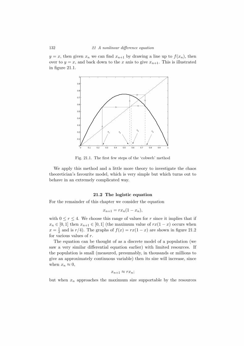
21.1.1 ‘Cobweb’ diagrams

In order to work out what happens when we iterate f , i.e. apply it again and

again, we can use a graphical method. If we draw the graph of f(x) and of

132 21 A nonlinear difference equation

y = x, then given xn we can find xn+1 by drawing a line up to f(xn), then

over to y = x, and back down to the x axis to give xn+1. This is illustrated

in figure 21.1.

0 0.1 0.2 0.3 0.4 0.5 0.6 0.7 0.8 0.9 10

0.1

0.2

0.3

0.4

0.5

0.6

0.7

0.8

0.9

1

x1 x

2x

3x

4

Fig. 21.1. The first few steps of the ‘cobweb’ method

We apply this method and a little more theory to investigate the chaos

theoretician’s favourite model, which is very simple but which turns out to

behave in an extremely complicated way.

21.2 The logistic equation

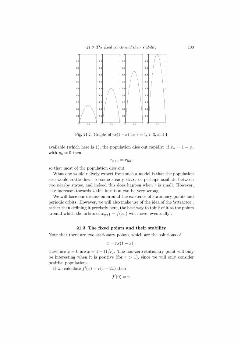
For the remainder of this chapter we consider the equation

xn+1 = rxn(1 − xn),

with 0 ≤ r ≤ 4. We choose this range of values for r since it implies that if

xn ∈ [0, 1] then xn+1 ∈ [0, 1] (the maximum value of rx(1 − x) occurs when

x = 1

2and is r/4). The graphs of f(x) = rx(1 − x) are shown in figure 21.2

for various values of r.

The equation can be thought of as a discrete model of a population (we

saw a very similar differential equation earlier) with limited resources. If

the population is small (measured, presumably, in thousands or millions to

give an approximately continuous variable) then its size will increase, since

when xn ≈ 0,

xn+1 ≈ rxn;

but when xn approaches the maximum size supportable by the resources

21.3 The fixed points and their stability 133

0 0.5 10

0.1

0.2

0.3

0.4

0.5

0.6

0.7

0.8

0.9

1

0 0.5 10

0.1

0.2

0.3

0.4

0.5

0.6

0.7

0.8

0.9

1

0 0.5 10

0.1

0.2

0.3

0.4

0.5

0.6

0.7

0.8

0.9

1

0 0.5 10

0.1

0.2

0.3

0.4

0.5

0.6

0.7

0.8

0.9

1

Fig. 21.2. Graphs of rx(1 − x) for r = 1, 2, 3, and 4

available (which here is 1), the population dies out rapidly: if xn = 1 − yn

with yn ≈ 0 then

xn+1 ≈ ryn,

so that most of the population dies out.

What one would naıvely expect from such a model is that the population

size would settle down to some steady state, or perhaps oscillate between

two nearby states, and indeed this does happen when r is small. However,

as r increases towards 4 this intuition can be very wrong.

We will base our discussion around the existence of stationary points and

periodic orbits. However, we will also make use of the idea of the ‘attractor’;

rather than defining it precisely here, the best way to think of it as the points

around which the orbits of xn+1 = f(xn) will move ‘eventually’.

21.3 The fixed points and their stability

Note that there are two stationary points, which are the solutions of

x = rx(1 − x) :

these are x = 0 are x = 1 − (1/r). The non-zero stationary point will only

be interesting when it is positive (for r > 1), since we will only consider

positive populations.

If we calculate f ′(x) = r(1 − 2x) then

f ′(0) = r,

134 21 A nonlinear difference equation

so the stationary point at x = 0 will be stable while r < 1, and unstable

once r > 1.

If 0 < r < 1 then there is no positive stationary point, and over time the

population decreases to zero, since the reproductive rate is not high enough

to sustain the population. So in this case the dynamics is very simple, and

the attractor is just zero. As remarked above, x = 0 is stable. (See figure

21.3.)

0 0.1 0.2 0.3 0.4 0.5 0.6 0.7 0.8 0.9 10

0.1

0.2

0.3

0.4

0.5

0.6

0.7

0.8

0.9

1logistic map with r=0.8

Fig. 21.3. For 0 < r < 1 the origin is a stable stationary point, and the populationdies out

When r > 1 the origin is no longer stable, and there is another positive

stationary point. Since

f ′(1 − (1/r)) = r(1 − 2 + (2/r)) = 2 − r,

this stationary point is stable while r < 3. So for 1 < r < 3 all orbits are

attracted to 1 − (1/r), as shown in figure 21.4.

When r increases beyond 3 things become more complicated. The sta-

tionary point at 1 − (1/r) is now unstable, since the derivative of f there

has modulus larger than 1.

21.4 Periodic orbits

When r > 3 the solution no longer tends towards a stationary point: there

are only two of them, and both are unstable. Instead, if r is just a little

larger than three, almost every choice of initial condition (apart from either

stationary point) ends up cycling between two different values of x, as shown

in figure 21.5.

Here there are values x1 and x2 such that

f(x1) = x2 and f(x2) = x1,

21.4 Periodic orbits 135

0 0.1 0.2 0.3 0.4 0.5 0.6 0.7 0.8 0.9 10

0.1

0.2

0.3

0.4

0.5

0.6

0.7

0.8

0.9

1

Fig. 21.4. For 1 < r < 3 the origin is unstable, and there is an attracting non-zerostationary point

0 0.1 0.2 0.3 0.4 0.5 0.6 0.7 0.8 0.9 10

0.1

0.2

0.3

0.4

0.5

0.6

0.7

0.8

0.9

1Period 2 orbit

Fig. 21.5. For r > 3 there are periodic orbits of period 2. This picture has r =1 +

√5 ≈ 3.2361.

so that f2(x1) = x1. Such a pair of points is called a periodic orbit of period

2 or a period 2 orbit.

In general a periodic orbit of period k (or a period k orbit) is a sequence

of k values x1, . . . , xk such that

f(xj) = xj+1 = f(xj) for j = 1, . . . , n − 1 and f(xn) = x1,

so that iterates of x1 cycle around these k values for ever. [Strictly we also

need to make sure that f(xj) 6= x1 for j = 1, . . . , n − 1, so that k is the

‘minimal period’ of the orbit.]

If we try to find a period 2 orbit analytically then we want to find a value

of y such that if xn = y then xn+2 = y. So we want

y = f2(y)

136 21 A nonlinear difference equation

which is

y = r[ry(1 − y)][1 − ry(1 − y)]. (21.3)

This is a quartic (fourth order) equation for y; but since we know that

y = 0 and y = 1 − (1/r) must be solutions (they are stationary points

with f(y) = y, so certainly f(f(y)) = f(y) = y) we can remove a factor

r(r − [1 − (1/r)]): if y is a period 2 point it must solve the equation

ry2 − (1 + r)y +

(

1 +1

r

)

= 0.

This equation only has real roots if the discriminant is positive (“b2 −4ac >

0”), i.e. if

(1 + r)2 − 4r

(

1 +1

r

)

= (1 + r)(r − 3) > 0.

Since we have restricted to the parameter range to 0 ≤ r ≤ 4 the first factor

is positive; for a period 2 orbit we must have r > 3.

21.5 Orbits beyond period 2

Insert picture here: r values: 0.5, 2, 3, 3.01, 3.5, 3.55, 3.565, 3.5701, 3.9, 4

As r is increased a little further, this attracting periodic orbit of period 2

becomes unstable - two points break off from each point on the orbit, and

we end up with an orbit of period 4, as shown in figure 21.6.

In order to see why this might happen, we consider what happens when

we apply f twice, i.e. we look at the graph of f 2. When r < 3 we have

a picture like that shown in figure 21.7 (the graph shows the diagonal, f ,

and f2). Both of the boxes are mapped into themselves when we apply f 2.

Magnifying the right-hand box we get figure 21.8, which looks very similar

to our logistic map when r < 1 (no stationary point except the origin).

However, when r > 3 the graph of f 2 has changed considerably, as shown

in figure 21.9. Blowing up the right-hand box again gives figure 21.10, which

now looks the logistic map with a stationary point.

By the time we reach r = 4 the graph of f 2 is shown in figure 21.11, and

the right-hand box magnified in figure 21.12: the top of the curve has gone

right out of the box.

So as we increase r we also increase the height of the bit of f 2 in the

right-hand box. So we expect that the dynamics of f 2 restricted to this box

will undergo the same changes of behaviour that happen to the dynamics

21.5 Orbits beyond period 2 137

0 0.1 0.2 0.3 0.4 0.5 0.6 0.7 0.8 0.9 10

0.1

0.2

0.3

0.4

0.5

0.6

0.7

0.8

0.9

1

Fig. 21.6. A period 4 orbit when r = 3.45

0 0.1 0.2 0.3 0.4 0.5 0.6 0.7 0.8 0.9 10

0.1

0.2

0.3

0.4

0.5

0.6

0.7

0.8

0.9

1graph of f2 when r=2.5

Fig. 21.7. Graph of f2 when r = 2.5

of f as we increase r. This idea, known as ‘renormalisation’, enables us to

understand what happens in great detail, and is also an important idea in

theoretical physics when studying phase transitions (liquid/solid, liquid/gas,

etc.)

The sketchy version given here goes at least some wasy to explain why

we would expect the period 2 orbit to become unstable and turn into an

attracting period 4 orbit. But we could then do the same with f 4 and find

a period 8 orbit... This period doubling cascade continues, creating, faster

and faster as we increase parameters, periods of order 2n, until at a critical

138 21 A nonlinear difference equation

0.6 0.62 0.64 0.66 0.68 0.7 0.72 0.74 0.76 0.78 0.80.6

0.62

0.64

0.66

0.68

0.7

0.72

0.74

0.76

0.78

0.8graph of f2 when r=2.5

Fig. 21.8. The right-hand box of figure 21.7 magnified

0 0.1 0.2 0.3 0.4 0.5 0.6 0.7 0.8 0.9 10

0.1

0.2

0.3

0.4

0.5

0.6

0.7

0.8

0.9

1graph of f2 when r=3.5

Fig. 21.9. Graph of f2 when r = 3.5

parameter value, r ≈ 3.5701, there are periodic orbits of orders 2n for every

n.

The universal property that can be obtained from the renormalisation

theory relates the convergence of the parameter values rn at which the orbit

of period 2n becomes unstable,

limn→∞

rn − rn−1

rn+1 − rn

= 4.667 . . . ,

and this number, ‘Feigenbaum’s constant’, is independent of the map, pro-

vided that (in a well-defined way) it ‘looks like’ our map f(x) = rx(1 − x).

[In fact it has to be a ‘one-hump map with a quadratic maximum’.]

21.6 The bifurcation diagram and more periodic orbits 139

0.72 0.74 0.76 0.78 0.8 0.82 0.84 0.86 0.88 0.9

0.72

0.74

0.76

0.78

0.8

0.82

0.84

0.86

0.88

0.9

graph of f2 when r=3.5

Fig. 21.10. The right-hand box of figure 21.9 magnified

0 0.1 0.2 0.3 0.4 0.5 0.6 0.7 0.8 0.9 10

0.1

0.2

0.3

0.4

0.5

0.6

0.7

0.8

0.9

1graph of f2 when r=4

Fig. 21.11. Graph of f2 when r = 4

21.6 The bifurcation diagram and more periodic orbits

Figure 21.13 is the bifurcation diagram that plots the attractor (vertically)

against the parameter r.

You can see the first few bits of the period doubling cascade before the

parameters become too close to distinguish. After r ≈ 3.5701 everything

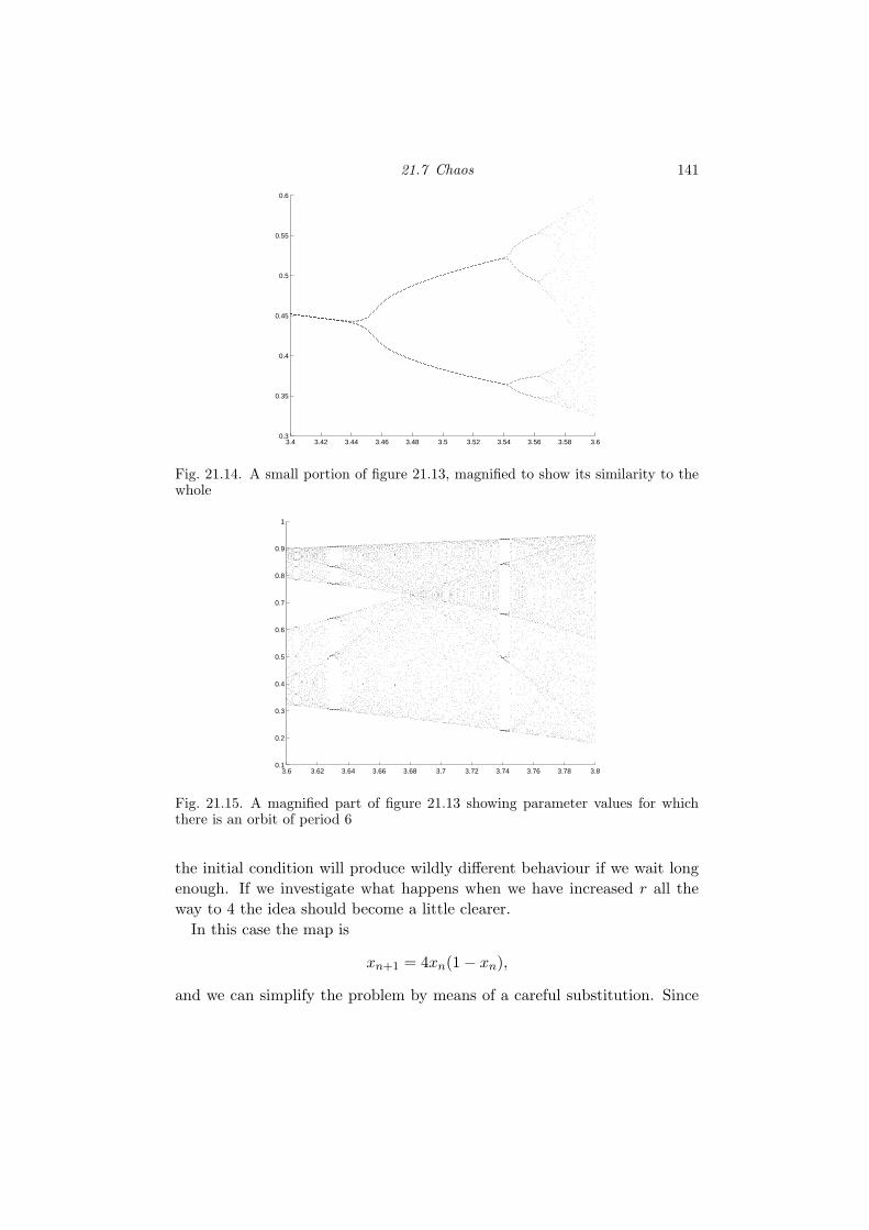
just starts to look a mess. However, there is still order. For example, you

can see that this diagram is ‘self-similar’ by magnifying a small portion and

observing that it looks very similar to the original diagram, as shown in

figure 21.14.

Notice also that there are ‘windows’ in which the solution is more regular

again - you can see one in figure 21.15 here where there is a period 6 orbit.

By the same mechanism that produces the orbits of period 4, 8, etc. from

140 21 A nonlinear difference equation

0.76 0.78 0.8 0.82 0.84 0.86 0.88 0.9 0.92

0.76

0.78

0.8

0.82

0.84

0.86

0.88

0.9

0.92

graph of f2 when r=4

Fig. 21.12. The right-hand box of figure 21.11 magnified

2.8 3 3.2 3.4 3.6 3.8 40

0.1

0.2

0.3

0.4

0.5

0.6

0.7

0.8

0.9

1

Value of r

Non

−w

ande

ring

poin

ts

Bifurcation diagram for logistic map

Fig. 21.13. The bifurcation diagram for 0 ≤ r ≤ 4

the initial period 2 orbit, this period 6 orbit will period double to 12, 24, 48,

and lead to another chaotic region, as you can see from the enlarged picture.

Insert picture here: bifurcations: 0:4, 2.9:3.6, 3.55:3.58 ylim([0.3 0.4]), 3.6:4, 3.83:3.86 ylim([0.4 0.6])

21.7 Chaos

Exactly what ‘chaos’ is is not entirely clear, since the literature contains

many definitions. Essentially it is deterministic motion in which the motion

appears to be random - and one auxiliary of this is that small changes to

21.7 Chaos 141

3.4 3.42 3.44 3.46 3.48 3.5 3.52 3.54 3.56 3.58 3.60.3

0.35

0.4

0.45

0.5

0.55

0.6

Fig. 21.14. A small portion of figure 21.13, magnified to show its similarity to thewhole

3.6 3.62 3.64 3.66 3.68 3.7 3.72 3.74 3.76 3.78 3.80.1

0.2

0.3

0.4

0.5

0.6

0.7

0.8

0.9

1

Fig. 21.15. A magnified part of figure 21.13 showing parameter values for whichthere is an orbit of period 6

the initial condition will produce wildly different behaviour if we wait long

enough. If we investigate what happens when we have increased r all the

way to 4 the idea should become a little clearer.

In this case the map is

xn+1 = 4xn(1 − xn),

and we can simplify the problem by means of a careful substitution. Since

142 21 A nonlinear difference equation

0 0.1 0.2 0.3 0.4 0.5 0.6 0.7 0.8 0.9 10

0.1

0.2

0.3

0.4

0.5

0.6

0.7

0.8

0.9

1Chaos in the logistic map when r=4

Fig. 21.16. Chaotic trajectories of xn+1 = 4xn(1 − xn)

xn ∈ [0, 1], we can set xn = sin2 θn, with θn ∈ [0, π/2]. The equation for θn

is then

sin2 θn+1 = 4 sin2 θn cos2 θn

= sin2(2θn).

Since we want θ ∈ [0, π/2], we can take

θn+1 =

{2θn 0 ≤ θn ≤ π/4

π − 2θn π/4 < θn ≤ π/2.

If we rescale, setting yn = 2θn/π, we obtain

yn+1 =

{2yn 0 ≤ 1

2

2(1 − yn) 1

2< yn ≤ 1.

and the new map is shown in figure 21.17.

The easiest way to consider the dynamics of this new map is by writing

down the binary decimal expansion of yn,

yn = [a1a2a3a4 . . .],

with

yn =∑

an2−n.

Then doubling yn corresponds to removing the first term,

yn+1 = [a2a3a4a5 . . .],

and subtracting 2yn from 2 is the same except we then have to switch all the

1s and 0s. If we denote this operation by a, then if yn > 1/2, i.e. if a1 = 1,

yn+1 = [a2a3a4a5 . . .].

21.7 Chaos 143

0 0.1 0.2 0.3 0.4 0.5 0.6 0.7 0.8 0.9 10

0.1

0.2

0.3

0.4

0.5

0.6

0.7

0.8

0.9

1Tent map for θ

Fig. 21.17. The ‘tent map’ obtained from our original map by a substitution

So we can write

if yn = [a1a2a3a4 . . .] then yn+1 =

{[a2a3a4a5 . . .] for a1 = 0

[a2a3a4a5 . . .] for a1 = 1.

First observe that there can be no stable periodic motions, since if y0 = y∗

implies that yn = y∗, then if y0 = y∗ + ε, assuming y∗ < 1/2 gives yn =

y∗ + 2nε, so that the trajectory moves away from the orbit. However, we

can show that all rational points are eventually periodic.

Just as in a decimal expansion, a rational number will have a repeating

or finite binary expansion. Thus any rational is eventually periodic, since

y0 = [b1b2b3b4b5 . . . bn(a1a2 . . . am)∞],

and so, changing a’s to a’s if necessary,

yn+1 = [(a1a2 . . . am)∞],

and then either fm(yn+1) = yn+1 or f2m(yn+1) = yn+1.

We have a strange situation, then. There are no stable orbits, but all

rational numbers are eventually periodic. Any number that starts irrational

will have a binary expansion, and hence an orbit, that never repeats itself.

One can also show that the distribution of points along an orbit is effectively

random, even though the evolution is deterministic. This model is now very

well understood, and is one of the standard examples used in dynamical

systems.

There are two deductions to be made from this investigation, one straight-

forward, but the other much more enlightening. The straightforward deduc-

tion is that very simple models can have extremely complicated behaviour.

144 21 A nonlinear difference equation

This is not, however, cause to despair at mathematical modelling, but indi-

cates the far more important principle that observed behaviour that is ex-

tremely complicated may in fact arise from extremely simple causes. Since

the advent of chaos theory, experimental data that was once discarded as

spurious and useless has been re-analysed and found, nevertheless, to contain

a high degree of order.