21-268: Multi-dimensional CalculusSpring 2012

Department of Mathematical-Sciences,Carnegie Mellon University.

Copyright 2012–2015, Department of Mathematical Sciences, Carnegie Mellon University.

This work is licensed under the Creative Commons Attribution-Non Commercial-Share Alike4.0 International License. This means you may adapt and or redistribute this documentfor non commercial purposes, provided you give appropriate credit and re-distributeyour work under the same licence. To view the full terms of this license, visit http://creativecommons.org/licenses/by-nc-sa/4.0/ or send a letter to Creative Com-mons, PO Box 1866, Mountain View, CA 94042, USA.

Preface ii

Preface

These notes were typed in 2012 when 21-268: Multi-dimensional Calculus wastaught by Russell Schwab in the Department of Mathematical-Sciences at Carnegie-Mellon university. The notes were typed by Christopher Almost.

These notes are being distributed by the Department of Mathematical-Sciencesas a service to the community, under the Creative Commons Attribution-Non Commercial-Share Alike 4.0 International License. This means you may adapt and or redis-tribute this document for non commercial purposes, provided you give appro-priate credit and re-distribute your work under the same licence. This means:

1. You may use these as lecture notes for a similar course you are teaching,provided you follow the licence terms.

2. You may give these notes to your students as a references, provided youfollow the licence terms.

3. You may edit these notes, and redistribute your modifications, provided youdo so under the same licence.

4. If however, you would like to use material in these notes for a commercialbook, you must obtain written prior approval.

To view the full terms of this license, visit http://creativecommons.org/licenses/by-nc-sa/4.0/ or send a letter to Creative Commons, PO Box 1866,Mountain View, CA 94042, USA.

The LATEX source for these notes is currently publicly hosted at GitLab: https://gitlab.com/gi1242/cmu-math-268. If you are interested in modifyingthese notes, please contact the current maintainer to discuss the best method.

These notes are provided as is, without any warranty and Carnegie MellonUniversity, the Department of Mathematical-Sciences, nor any of the authors areliable for any errors.

Contents

Preface ii

Contents iii

0 Linear algebra review 1

1 Functions of several real variables 11.1 Examples of multi-dimensional functions . . . . . . . . . . . . . . . . 11.2 Notation and basic definitions . . . . . . . . . . . . . . . . . . . . . . . 21.3 Limits and continuity . . . . . . . . . . . . . . . . . . . . . . . . . . . . . 3

2 Differentiation of multi-dimensional functions 52.1 Best affine approximation and partial derivatives . . . . . . . . . . . 52.2 Linearization and the Jacobian matrix . . . . . . . . . . . . . . . . . . 72.3 Rules of Differentiation . . . . . . . . . . . . . . . . . . . . . . . . . . . 9

3 Geometric applications 103.1 Curves and paths . . . . . . . . . . . . . . . . . . . . . . . . . . . . . . . 103.2 Paths on surfaces . . . . . . . . . . . . . . . . . . . . . . . . . . . . . . . 11

4 Higher derivatives and Taylor’s theorem 134.1 Higher derivatives . . . . . . . . . . . . . . . . . . . . . . . . . . . . . . 134.2 Extrema and the second derivative test . . . . . . . . . . . . . . . . . 194.3 Constrained extrema and Lagrange multipliers . . . . . . . . . . . . . 21

5 Multi-dimensional integrals 235.1 Double integrals . . . . . . . . . . . . . . . . . . . . . . . . . . . . . . . . 235.2 Triple integrals . . . . . . . . . . . . . . . . . . . . . . . . . . . . . . . . 265.3 Riemann sums . . . . . . . . . . . . . . . . . . . . . . . . . . . . . . . . . 295.4 Changes of coordinates . . . . . . . . . . . . . . . . . . . . . . . . . . . 305.5 Polar coordinates . . . . . . . . . . . . . . . . . . . . . . . . . . . . . . . 305.6 Spherical Coordinates . . . . . . . . . . . . . . . . . . . . . . . . . . . . 31

6 Integrals over paths and surfaces 326.1 Line and path integrals . . . . . . . . . . . . . . . . . . . . . . . . . . . 326.2 Parameterized surfaces . . . . . . . . . . . . . . . . . . . . . . . . . . . 346.3 Surface integral . . . . . . . . . . . . . . . . . . . . . . . . . . . . . . . . 36

7 Vector Calculus 367.1 Divergence and curl . . . . . . . . . . . . . . . . . . . . . . . . . . . . . 377.2 Orientation of boundaries . . . . . . . . . . . . . . . . . . . . . . . . . . 387.3 Flux and Gauss’ theorem . . . . . . . . . . . . . . . . . . . . . . . . . . 417.4 Stoke’s theorem . . . . . . . . . . . . . . . . . . . . . . . . . . . . . . . . 427.5 Proof of Stoke’s theorem for a graph . . . . . . . . . . . . . . . . . . . 43

iii

Contents iv

7.6 Gauss’ theorem . . . . . . . . . . . . . . . . . . . . . . . . . . . . . . . . 45

Index 48

Linear algebra review 1

0 Linear algebra review

1. (a) Recall that λ and v are respectively an eigenvalue and associated eigen-vector of the linear map T if. . . If v 6= 0 and T v = λv.

(b) Implicitly, assumptions were made in (a) about the domain and rangeof T . What were they? They must be the same vector space.

2. Find the eigenvalues of A =

−2 50 4

. They are −2 and 4 because A is uppertriangular and those are the diagonal elements.

3. Let p ∈ Rn be a fixed, non-zero, vector.(a) What space should v be in for p · v to make sense? The dual space ofRn, which is canonically isomorphic to Rn.

(b) What is the solution space of all v with p · v = 0? Is it a vector space?Why? What is the dimension, and why? It is the hyperplane of all vectorsperpendicular to p, a vector space of dimension n− 1.

4. (a) To which diagonal matrix, say B, is A in question 2 similar (conjugate)?It is similar to B =

−2 00 4

because its eigenvalues are distinct and henceA is diagonalizable.

(b) What does it mean for two matrices to be similar (conjugate)? A issimilar to B if there is an invertible matrix M (a change of basis) suchthat A= M−1BM.

5. Suppose D is similar (conjugate) to

C =

−1 0 00 2 00 0 1

.

Evaluate det(D) and tr(D). They are −2 and 2, respectively, because those arethe answers for C, and both det and tr are invariant for conjugation.

6. Does it make sense to talk about eigenvectors of

E =

2 1 0 10 1 0 01 −1 0 1

.

Why or why not? No, because the domain of E is R4 but its range is R3, whichare not the same space.

1 Functions of several real variables

1.1 Examples of multi-dimensional functions

We know how to do calculus for functions f : R→ R or f : [a, b]→ R of a singlereal variable. Here are some examples of functions with more inputs and outputsthan just one.

1.2. Notation and basic definitions 2

1.1.1 Examples.1. Temperature in a physical space (e.g. this room). The input is the Cartesian

coordinate of the point in the room, x = (x1, x2, x3), and the output is T (x),the temperature. Here T : R3→ R or T : Ω ⊆ R3→ R.

2. Topographical height on a map or on the Earth’s surface. The input is thecoordinates x = (x1, x2), or longitude and latitude, and the output is theheight, h(x). Here h : R2→ R or h : S2→ R, where S2 is the 2-dimensionalsphere.

3. Electrostatic potential Φ and electric field E. The input is the coordinates,x , of a point in a physical space and the outputs are Φ : R3 → R, the scalarelectric potential (voltage) at x , and E : R3→ R3, the vector indicating forceon a particle due to electric field. We will see that, typically, E = DΦ, thegradient of Φ, a topic of this course.

4. From economics, the utility function U . The inputs are the amounts of eachgood you could consume (e.g. hours at a pinball machine, number of ap-ples, number of oranges, amount of fizzy beverage, etc.) The ouput is thescalar quantity that is the amount of “satisfaction” derived from that particu-lar choice of consumption bundle. Here U : Rn

+→ R, where n is the numberof goods under consideration. R+ = [0,∞) is the collection of non-negativereal numbers.

1.2 Notation and basic definitions

We need to define some notation that makes analogy with the idea of a function ofa single variable f : [a, b]→ R in 1-dimensional calculus. The underlying space forthis course is Rn, n-tuples of real numbers, with canonical basis e1, . . . , en, whereei is the n-vector with a 1 in the ith position and zeros everywhere else.

The inner product on Rn is defined by

⟨x , y⟩ := x · y = x1 y1 + · · ·+ xn yn.

This defines a distance on Rn defined by d(x , y)2 := ⟨x − y, x − y⟩, the squaredlength of x − y . We will also write |x − y| := d(x , y) (absolute value bars). So thenorm on Rn is defined by |x |2 = ⟨x , x⟩. Yet otherwise said,

|x − y|= d(x , y) =

√

√

√

n∑

i=1

(x i − yi)2.

An ε-neighbourhood of x ∈ Rn is Bε(x) := y ∈ Rn : d(x , y) < ε, the ball centredat x with radius ε, not including the boundary (i.e. the open ball).

A subset Ω ⊆ Rn is an open set if for all x ∈ Ω, there is some neighbourhood ofx also contained in Ω (i.e. there is ε > 0 such that Bε(x) ⊆ Ω). This generalizes theidea that if x ∈ (a, b) then there is always “room” between a and x and betweenx and b. A subset Ω ⊆ Rn is closed set if its complement Ωc := Rn \Ω is an openset. In symbols, for all y /∈ Ω there is some ε > 0 such that Bε(y)∩Ω=∅.

1.3. Limits and continuity 3

1.2.1 Example. Ω := x ∈ R2 : |x1| ≤ 1 and |x2| ≤ 1 is closed. It is the closedbox/square [−1,1]×[−1, 1]. For any y outside of Ω (so |y1|> 1 or |y2|> 1) thereis ε > 0 such that Bε(y) does not intersect the square.

A subset Ω ⊆ Rn is bounded if there is some R > 0 such that Ω ⊆ BR(0). (Notethat you should be able to tell that R is a scalar from the context: the only collectionin this course for which we will define a total ordering “<” is R.)

1.2.2 Examples.1. Ω := x ∈ Rn : |x i | ≤ 1 for all i = 1, . . . , n is bounded. Taking R :=

p8

shows this.2. Ω := x ∈ R2 : x1 x2 < 1 is the region “between” two hyperbolas in R2. Ω

is not bounded. Indeed, it contains the line x2 = −x1.3. Vector subspaces of Rn are not bounded sets. In general they are not open

sets either.

A subset Ω ⊆ Rn is connected (actually path-connected) if, for all x , y ∈ Ω, thereis a path γ from x to y . (A path γ is a continuous function γ : [a, b] → Rn, andγ is said to go from x to y if γ(a) = x and γ(b) = y .) For open sets, it sufficesto replace “path γ” in the definition of connected with “an ordered collection ofunbroken straight line segments starting at x and ending with y .”

We will say that Ω is a domain if it is open and (path-)connected. Domains arethe sets over which we will do multi-variable calculus.

1.2.3 Example. Consider the following function f : R2 \ 0 → R defined by

f (x1, x2) :=x2

1 − x22

x21 + x2

2

.

What does the graph of f look like? Is f “well-behaved” near x = 0?We have several tools at our disposal. The level curves of f are the sets x ∈

R2 \ 0 : f (x) = c for various choices of c. The level set for c = 0 is the pair oflines x1 = x2 and x1 = −x2 (not including zero). The level sets for c = 1 and −1are the lines x2 = 0 and x1 = 0, respectively. In polar coordinates,

f (r,θ ) =(r cosθ )2 − (r sinθ )2

r2= cos(2θ ).

Interestingly, this formula does not depend on the radius.

1.3 Limits and continuity

This section follows K§2.4. We saw that the function from Example 1.2.3 wasnot so well-behaved for its argument near zero, in the sense that the values thefunction takes on a circle centred at the origin are cos(2θ ), irrespective of theradius. Continuity is the property of a function, say f , that the values f (x) can bemade as close to f (x0) as we like by taking x close to x0. The precise definition isas follows. Let f : Ω ⊆ Rn→ Rm be a function.

1.3. Limits and continuity 4

1.3.1 Definition. We say that limx→x0f (x) = c, that f has a limit of c at x0 ∈ Ω

or x0 on the boundary of Ω, if for all ε > 0 there is δ > 0 such that | f (x)− c| < εfor every x ∈ Ω such that 0 < |x − x0| < δ. Note that we do not require that thishold at x = x0. This is the δ-ε definition of limit. We say that f is continuous atx0 ∈ Ω if limx→x0

f (x) = f (x0).

If the domain of f is R then there are only two directions from which to ap-proach a point x0 – from the left or from the right. In Rn there are many ways toapproach a point, and more than just the 2n ways along the coordinate directions.

1.3.2 Example. Let f be as in Example 1.2.3 and define

g(x) =

¨

f (x), x 6= 0

0, x = 0.

Let’s try x → x0 for a few different 1-dimensional approaches. Let

γ(s) = (x1(s), x2(s))

for the following choices of γ.1. If γ(s) = (s, 0) then

lims→0

g(γ(s)) = lims→0

s2

s2= 1.

2. If γ(s) = (0, s) then

lims→0

g(γ(s)) = lims→0

−s2

s2= −1.

3. If γ(s) = (s, s) then

lims→0

g(γ(s)) = lims→0

02s2= 0.

4. If γ(s) = (s cos s, s sin s) then lims→0 g(γ(s)) = lims→0 cos(2s) = 1.5. Think of a function γ for which lims→0 g(γ(s)) does not exist.

1.3.3 Exercises.1. Let γ(s) = (s cos( 1

s ), s sin( 1s )) and s(0) = 0. Describe the path γ. Is is contin-

uous at s = 0? Yes, it is continuous at s = 0 because

lims→0|γ(s)|= lim

s→0

Ç

s2 cos2( 1s ), s2 sin2( 1

s ) = lims→0

s = 0= γ(0).

The path γ spirals around (0, 0), making infinitely many complete turns aroundit before reaching zero.

2. What happens with f (x) = (x21 − x2

2)/(x21 + x2

2) under s 7→ f (γ(s))? Doeslims→0 f (γ(s)) exist? The limit does not exist because f (γ(s)) = cos( 2

s ), whichis very badly behaved near s = 0.

Differentiation of multi-dimensional functions 5

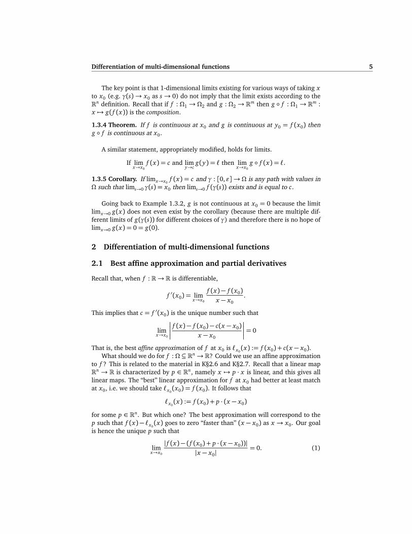
The key point is that 1-dimensional limits existing for various ways of taking xto x0 (e.g. γ(s)→ x0 as s→ 0) do not imply that the limit exists according to theRn definition. Recall that if f : Ω1 → Ω2 and g : Ω2 → Rm then g f : Ω1 → Rm :x 7→ g( f (x)) is the composition.

1.3.4 Theorem. If f is continuous at x0 and g is continuous at y0 = f (x0) theng f is continuous at x0.

A similar statement, appropriately modified, holds for limits.

If limx→x0

f (x) = c and limy→c

g(y) = ` then limx→x0

g f (x) = `.

1.3.5 Corollary. If limx→x0f (x) = c and γ : [0,ε]→ Ω is any path with values in

Ω such that lims→0 γ(s) = x0 then lims→0 f (γ(s)) exists and is equal to c.

Going back to Example 1.3.2, g is not continuous at x0 = 0 because the limitlimx→0 g(x) does not even exist by the corollary (because there are multiple dif-ferent limits of g(γ(s)) for different choices of γ) and therefore there is no hope oflimx→0 g(x) = 0= g(0).

2 Differentiation of multi-dimensional functions

2.1 Best affine approximation and partial derivatives

Recall that, when f : R→ R is differentiable,

f ′(x0) = limx→x0

f (x)− f (x0)x − x0

.

This implies that c = f ′(x0) is the unique number such that

limx→x0

f (x)− f (x0)− c(x − x0)x − x0

= 0

That is, the best affine approximation of f at x0 is `x0(x) := f (x0) + c(x − x0).

What should we do for f : Ω ⊆ Rn→ R? Could we use an affine approximationto f ? This is related to the material in K§2.6 and K§2.7. Recall that a linear mapRn → R is characterized by p ∈ Rn, namely x 7→ p · x is linear, and this gives alllinear maps. The “best” linear approximation for f at x0 had better at least matchat x0, i.e. we should take `x0

(x0) = f (x0). It follows that

`x0(x) := f (x0) + p · (x − x0)

for some p ∈ Rn. But which one? The best approximation will correspond to thep such that f (x)− `x0

(x) goes to zero “faster than” (x − x0) as x → x0. Our goalis hence the unique p such that

limx→x0

| f (x)− ( f (x0) + p · (x − x0))||x − x0|

= 0. (1)

2.1. Best affine approximation and partial derivatives 6

But how do we do this? Note that x 7→ p · x is a linear map Rn→ R. To knowp, we need to know pi for i = 1, . . . , n. But p · ei = pi , so we need only look in thedirections of the canonical basis. Whence, for small h ∈ R,

`x0(x0 + hei) = f (x0) + p · (x0 + hei − x0) = f (x0) + hpi ,

From the definition of the derivative, with x = x0 + hei ,

0= limx→x0

| f (x)− ( f (x0) + p · (x − x0))||x − x0|

= limh→0

| f (x0 + hei)− ( f (x0) + hp · ei)|h

= limh→0

f (x0 + hei)− f (x0)h

− pi

It follows that

pi = limh→0

f (x0 + hei)− f (x0)h

This is the 1-dimensional derivative of the function g(h) := f (x0 + hei). Think ofg as the restriction of f to the 1-dimensional space x0 + span(ei).

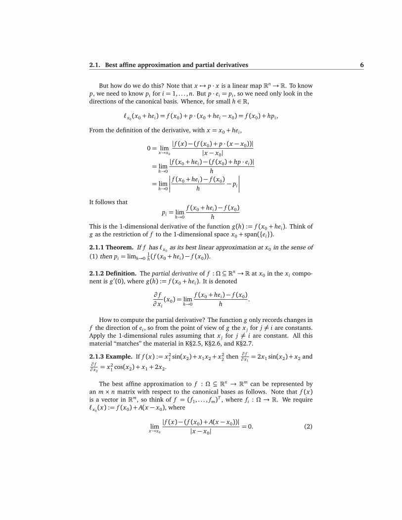
2.1.1 Theorem. If f has `x0as its best linear approximation at x0 in the sense of

(1) then pi = limh→01h ( f (x0 + hei)− f (x0)).

2.1.2 Definition. The partial derivative of f : Ω ⊆ Rn→ R at x0 in the x i compo-nent is g ′(0), where g(h) := f (x0 + hei). It is denoted

∂ f∂ x i(x0) = lim

h→0

f (x0 + hei)− f (x0)h

.

How to compute the partial derivative? The function g only records changes inf the direction of ei , so from the point of view of g the x j for j 6= i are constants.Apply the 1-dimensional rules assuming that x j for j 6= i are constant. All thismaterial “matches” the material in K§2.5, K§2.6, and K§2.7.

2.1.3 Example. If f (x) := x21 sin(x2)+ x1 x2+ x2

2 then ∂ f∂ x1= 2x1 sin(x2)+ x2 and

∂ f∂ x2= x2

1 cos(x2) + x1 + 2x2.

The best affine approximation to f : Ω ⊆ Rn → Rm can be represented byan m × n matrix with respect to the canonical bases as follows. Note that f (x)is a vector in Rm, so think of f = ( f1, . . . , fm)T , where fi : Ω → R. We require`x0(x) := f (x0) + A(x − x0), where

limx→x0

| f (x)− ( f (x0) + A(x − x0))||x − x0|

= 0. (2)

2.2. Linearization and the Jacobian matrix 7

If this holds then A is unique and A= (ai j)i=1,...,m, j=1,...,n, where ai j = [Aei] j is theith component of the vector Ae j ∈ Rm. To isolate ai j we perform the same basicprocedure as in the Rn→ R case, but applied to the ith entries of `x0

and f .

[ f (x0 + he j)− f (x0)− A(x0 + he j − x0)]i = [ f (x0 + he j)− f (x0)− hAe j]i= fi(x0 + he j)− fi(x0)− [hAe j]i

But this gives exactly the partial derivative of fi in the x j direction, i.e.

ai j =∂ fi

∂ x j= lim

h→0

fi(x0 + he j)− fi(x0)

h

for i = 1, . . . , m and j = 1, . . . , n.

2.2 Linearization and the Jacobian matrix

We say that f : Ω ⊆ Rn → Rm is total differentiable or full differentiable at x0 ifthere is an m× n matrix A such that (2) holds. We write D f (x0) = A. This matrixis also known as the Jacobian of f at x0.

2.2.1 Theorem. If f is full differentiable at x0 then ∂ fi∂ x j(x0) exists and is equal to

[D f (x0)]i j , the (i j)th entry of A.

But when is A given by the partials?

2.2.2 Theorem. Let f : Ω ⊆ Rn→ Rm, x0 ∈ Ω, and ε > 0 be such that Bε(x0) ⊆ Ω.If ∂ fi∂ x j

all exist and are continuous on Bε(x0) then f is full differentiable at x0 and

[D f (x0)]i j =∂ fi∂ x j(x0).

Note that | · |Rm controls the norms | · |R of each of the components of f ∈ Rm

and also of x ∈ Rn. So (2) is very strong. The information about fi(x0 + he j) asfunctions R→ R is not enough to get the full derivative. But the extra requirementthat ∂ fi

∂ x jexist and are continuous on a whole neighbourhood is enough.

2.2.3 Example. limx→0 cos( 1x ) does not exist. If the limit did exists, say was c,

then c ∈ [−1,1] because that is the range of the function cosine. Suppose thatc 6= 1. Let ε := 1

2 |1− c| > 0. Then ε > 0 and we will show that there is no δ > 0such that | cos( 1

x )− c| < ε for all |x | < δ. Let xn := 12πn . Then xn → 0 as n→∞

and

| cos( 1xn)− c|= | cos(2πn)− c|= |1− c|>

12|1− c|= ε.

Therefore, no matter which δ > 0 we try, there is n large enough that |xn| < δ,and | cos( 1

xn) − c| > ε. Therefore c is not the limit, so either 1 is the limit or the

limit does not exist. But repeating the same argument with the assumption thatc 6= −1 and xn := 1

π(2n+1) shows that the limit cannot be 1, so the limit does notexist.

2.2. Linearization and the Jacobian matrix 8

We have seen that the existence of a “best affine approximation” implies thatthe partial derivatives exist. That is to say, given f : Ω ⊆ Rn → R and x0 ∈ Ω, ifthere is a unique p ∈ Rn such that

limx→x0

| f (x)− f (x0)− p · (x − x0)||x − x0|

= 0.

(this is (1) again), then f has partial derivatives in all directions at x0. We haveseen that `x0

(x) := f (x0)+ p · (x − x0) is the best affine approximation to f at x0.Functions f for which a best affine approximation exist are said to be differentiable.Not all functions are differentiable.

Taking x = x0 + he j and plugging it into (1),

0= limx→x0

| f (x)− `x0(x)|

|x − x0|

= limh→0

| f (x0 + he j)− f (x0)− p · (he j)||he j |

x − x0 = he j

= limh→0

| f (x0 + he j)− f (x0)− hp · e j ||h|

|e j |= 1

= limh→0

f (x0 + he j)− f (x0)− hp · e j

h

ratio of real numbers

0= limh→0

f (x0 + he j)− f (x0)

h− p · e j

p · e j = limh→0

f (x0 + he j)− f (x0)

h

This tells us both that the limit on the right exists and that it is equal to p · e j = p j .

We write D f (x0) = p and ∂ f∂ x j(x0) = p j . We call D f the gradient of f at x0 (but only

when f maps toR, in which case D f is an n-vector). The best affine approximationto f at x0 can hence be rewritten as

`x0(x) = f (x0) + D f (x0) · (x − x0)

= f (x0) +∂ f∂ x1(x0)(x1 − x01) + · · ·+

∂ f∂ xn(x0)(xn − x0n).

2.2.4 Example. Is f (x) := |x |=q

x21 + · · ·+ x2

n differentiable at x = 0? It is not,

because if it were then ∂ f∂ x1(0) would exist, but

f (0+ he1)− f (0)h

=p

h2

h= ±1

where the ± depends on the sign of h. Therefore the limit as h→ 0 does not exist,so the limit defining ∂ f

∂ x1(0) does not exist. This implies that f is not differentiable.

Similarly, g(x) = x21 + |x2| is not differentiable at x = 0 because ∂ f

∂ x2(0) does not

exist (though in this case ∂ f∂ x1(0) does exist).

2.3. Rules of Differentiation 9

In which direction does f increase the fastest from f (x0)? Hint: first thinkof which direction `x0

increases the fastest. Since f and `x0are “very close” in a

neighbourhood of x0, the answers should be the same.The tangent plane to the graph of f : Rn → R at x0 is the graph of the best

affine approximation `x0. It is the unique hyperplane that touches the graph of f

at x0 and which satisfies error(x − x0)/|x − x0| → 0 as x → x0.

2.3 Rules of Differentiation

As with 1-dimensional derivatives, there are a few rules that the derivative satisfies.1. If f : Ω ⊆ Rn→ Rm and c ∈ R then

D(c f )(x0) = cD f (x0).

2. If f , g : Ω→ R then

D(g f )(x0) = g(x0)D f (x0) + f (x0)Dg(x0).

3. If f , g : Ω→ Rm then

D( f + g)(x0) = D f (x0) + Dg(x0).

4. If g : Ω1 ⊆ R`→ Ω2 ⊆ Rm and f : Ω2→ Rn then

D( f g)(x0) = D f (g(x0))Dg(x0).

The last rule is the chain rule. It is one of the best reasons for using the “best affineapproximation” definition of the derivative.

g(x) = g(x0) + Dg(x0)(x − x0) + errg(x − x0)

f (g(x)) = f (g(x0)) + D f (g(x0))(g(x)− g(x0)) + err f (g(x)− g(x0))

= f (g(x0)) + D f (g(x0))[Dg(x0)(x − x0)+ errg(x − x0)] + err f (g(x)− g(x0))

= f (g(x0)) + D f (g(x0))Dg(x0)(x − x0)+ [D f (g(x0))errg(x − x0) + err f (g(x)− g(x0))]

Furthermore, because the errors in the best affine approximation go to zero fasterthan |x − x0| as x → x0,

limx→x0

|D f (g(x0))errg(x − x0) + err f (g(x)− g(x0))||x − x0|

= limx→x0

|D f (g(x0))|errg(x − x0)

|x − x0|+ lim

x→x0

err f (g(x)− g(x0))

|g(x)− g(x0)||g(x)− g(x0)||x − x0|

= 0

Make the previous computation precise as an exercise. Note that we have usedthe fact that g is continuous at x0 (to know that g(x)→ g(x0)) and also that g is

Geometric applications 10

differentiable at x0 (to know that the ratio |g(x)−g(x0)|/|x−x0| is bounded). Thisshows that D f (g(x0))Dg(x0) is the correct matrix for the best affine approximationof f g at x0. Check that the shapes are in fact correct for multiplying thesematrices together.

2.3.1 Exercise. Suppose f : Rn → R : x 7→ x + q · x . What is D f (x0) for any x0?It is always q because f is affine, so it is its own best affine approximation. Think off (x) = (c + q · x0) + q · (x − x0).

3 Geometric applications

Given a direction v (so |v| = 1), how does f change at x0 in the straight linethrough x0 in the direction v, i.e. in the affine space x0 + span(v)? This is a 1-dimensional problem. Let g(s) = x0+sv and use the chain rule on the compositionf (g(s)). Since Dg(0) = v and f (g(0)) = f (x0), the derivative is D f (x0) · v. Thisis the directional derivative of f at x0 in the direction v.

3.1 Curves and paths

Notation. C1(Ω) is the collection of functions f : Ω→ Rm such that D f (x) existsand is continuous for all x ∈ Ω. Typically Ω is an open connected set, i.e. a domain.Such functions are said to be continuously differentiable.

A path is a map γ : [a, b] → Rn. The terminology of continuity and differen-tiability carry over from what we have been discussing for the past few weeks. Wewill write γ′ := γ := Dγ for paths, when appropriate, and we refer to this n-vectoras the velocity vector. curve is the image left behind after tracing a path. Moreprecisely, it is the image of a path, Γ = γ([a, b]) = γ(t) : t ∈ [a, b]. Note thedifference between γ and Γ .

We say that Γ is differentiable at x0 ∈ Γ if there exists a continuously differen-tiable path γ : [a, b]→ Γ and t0 ∈ [a, b] such that both γ(t0) = x0 and γ′(t0) 6= 0.The tangent line is the unique line with direction γ′(t0) and which touches (i.e. istangent to) Γ at x0.

3.1.1 Examples.1. Let γ : [0,4π]→ R2 : t 7→ (t cos t, t sin t). The partial derivatives are

γ′1(t) = cos t − t sin t and γ′2(t) = sin t + t cos t,

which are both differentiable and never both zero. Indeed, the sum of theirsquares is 1+ t2. Hence the image of this path is a differentiable curve.[Insert sketch of the spiral.]

2. Consider now the path [−1,1]→ R2 : t 7→ (t4, t2). It is differentiable at allt ∈ (−1,1), but the image curve Γ is not differentiable at zero. It has a cuspat the origin.

3.2. Paths on surfaces 11

[Insert image. Note that γ2 =p

|γ1|.]To prove that the curve Γ is not differentiable at (0, 0), we must show

that any possible candidate γ : [a, b]→ Γ that is continuously differentiablefails the requirement that γ′(t0) 6= 0. By “shifting”, we may always assumewithout loss of generality that t0 = 0. Observe that all points x ∈ Γ satisfyx2 =

p

|x1|. Therefore γ(t) = (c(t),p

|c(t)|) for some c : [a, b] → R. Weare requiring that γ is continuously differentiable, so there is a best affineapproximation at zero, call it v = γ′(0), such that

0= limt→0

|γ(t)− γ(0)− v(t − 0)||t|

= limt→0

q

(c(t)− t v1)2 + (p

|c(t)| − t v2)2

|t|

≥ limt→0

q

(p

|c(t)| − t v2)2

|t|

= limt→0

|t|

p|c(t)|t − v2

|t|

= limt→0

p

|c(t)|t

− v2

Therefore we may conclude

v2 = limt→0

p

|c(t)|t

v22 = lim

t→0

|c(t)|t2

x 7→ x2 is continuous

limt→0

t v22 = lim

t→0

|c(t)|t

0= limt→0

|c(t)|t

0= limt→0

|c(t)− 0|t

Since γ is continuously differentiable, c′(0) exists, and by the limit above, itmust be zero. Can it be the case that c′(0) = 0 but (

p

|c(t)|)′(0) 6= 0? Again,since γ is continuously differentiable,

p

|c(t)| is differentiable at t = 0. Therest of the proof is an exercise.

3.2 Paths on surfaces

What is a surface? Intuitively, a surface is a 2-dimensional object inside of a 3-dimensional space, e.g. a piece of paper in this room, the surface of a ball (asphere), etc. More precisely, S ⊆ Rn+1 is a level surface if it can be written as

3.2. Paths on surfaces 12

S = x ∈ Rn+1 : F(x) = c, where F : Rn+1 → R is continuously differentiableand c is a fixed constant, and DF(x) 6= 0 for all x near S. In this case we say thedimension of S is n. Note that F : Rn+1→ R actually describing an n-dimensionalsurface is special. We must be careful with F , because not every such functiongives rise to an n-dimensional surface.

3.2.1 Examples.1. Justification for DF 6= 0. Let

F(x) =

¨

0, |x | ≤ 1

(|x | − 1)2, |x |> 1.

Then F is continuously differentiable. (Check this carefully for |x |= 1.)[Insert diagram of the 3-d picture of F .]Note x : F(x) = 0 = x : |x | ≤ 1 is not “1-dimensional” in the usual

sense of the term. DF(x) = 0 for all x in this level set, which is why weexclude this case.

2. Now let F(x) = |x |. Then DF(x) = x/|x | for all n 6= 0 and F is not differ-entiable at zero. For c > 0, the level surface associated with F and c is thecircle of radius c when n= 2 and the sphere of radius c when n= 3.

3. If f : R2 → R then the graph of f is x ∈ R3 : x3 = f (x1, x2). It canbe realized as a 2-dimensional surface by taking F : R3 → R with F(x) =f (x1, x2)− x3 and c = 0. Note that DF = ( ∂ f

∂ x1, ∂ f∂ x2

,−1) is never zero. Forexample, if f (x) = x2

1 − x22 then F(x) = x2

1 − x22 − x3.

4. Another way to find curves in R2 other than images of paths is level surfacesof F : R2 → R, i.e. a 1-dimensional level surface is basically a curve. Forexample, if F(x) = x2

1−s22 then the level surfaces are a tool for understanding

the graph of F . At c = 0 we have x21 − x2

2 = 0, so x1 = ±x2. For c = 1 weget x2

1 − x22 = 1, a hyperbola, and for c = −1, we get x2

1 − x22 = −1, another

hyperbola.[Insert diagram of level sets and of the 3-d picture.]

3.2.2 Example. Let γ : [0,1] → R3 : t 7→ (t cos(4πt), t sin(4πt),p

1− t2), andnote that |γ(t)| = 1 for all t. This means that γ happens to always take valueson the sphere S = x ∈ R3 : |x | = 1. The path of γ starts at the north pole att = 0 and spirals down in an anti-clockwise direction until it reaches the equatorat t = 1 after making two full revolutions.

In general, if γ is a path on a level surface S = x : F(x) = c then, necessarily,F(γ(t)) = c for every t in the domain of γ. A special case is a path on a graphof a function f : Rn → R. Recall that the graph of f is an n-dimensional surfacein Rn+1. If γ : [a, b] → Rn+1 is on the graph of f then it must be the case thatγ(t) = (γ1(t), . . . ,γn(t), f (γ(t))), i.e. the (n+1)st component of γ is related to thefirst n components by f .

What is the analog of the best affine approximation for surfaces? If the levelsurface is the graph of a function f , then we have seen that the tangent plane at a

Higher derivatives and Taylor’s theorem 13

point x0 is exactly the graph of the best affine approximation of f at x0. Basicallyall directional derivatives are encoded in the “slope” of the tangent plane.

We determined the partial derivatives by reducing to the 1-dimensional case.For each direction ei , we consider the function gi(h) = f (x0 + hei), so that thepartial derivatives are given by ∂ f

∂ x i(x0) = g ′(0). Note that gi is a path on the

graph of f that passes through x0! Furthermore, g ′(0) = D f (x0) · ei . This is goodmaterial with which to formulate a definition. We say that the tangent plane to thegraph of f is the unique plane which touches the graph at (x0, f (x0)) and containsthe velocity vectors, γi(0), of each of the paths γi(s) := (x0 + sei , f (x0 + sei)).

Now let S = x ∈ Rn+1 : F(x) = c be a level surface. We say that the tangentplane (or tangent hyperplane) to S at x0 ∈ S is the unique n-dimensional plane thatcontains x0 and x0+ γ(0) for every continuously differentiable path γ contained inS with γ(0) = x0. Recall that γ is a path in S if γ : [a, b]→ Rn+1 and γ(t) ∈ S for allt ∈ [a, b]. Equivalently, if F(γ(t)) = c for all t ∈ [a, b]. From this latter equation(and the chain rule) we will be able to calculate the equation of the tangent plane.Differentiating at t = 0,

0= DF(γ(0)) · γ(0) = DF(x0) · γ(0)

But how many choices are there for γ(0) as γ ranges over the collection of appro-priate paths? The tangent plane should contain all the directions solving DF(x0) ·p = 0, or equivalently and more precisely, the tangent plane is the affine spacex0 + (span(DF(x0)))⊥. Yet otherwise said, x is in the tangent plane to S atx0 ∈ S if and only if DF(x0) · (x − x0) = 0.

3.2.3 Example. Let S be the unit sphere inR3, S = x ∈ R3 : |x |= 1. The tangentplane at (1,0, 0) is computed as follows. In this case F(x) = |x |, so (compute asan exercise) DF(x) = x/|x |, and since x0 = (1,0, 0), DF(x0) = (1,0, 0).[Insert diagram?]The tangent plane is the unique plane perpendicular to (1, 0,0) containing

(1,0, 0). (It is a coincidence of the sphere that x0 = DF(x0).) More explicitly,the tangent plane is (1, s, t) : s, t ∈ R.

4 Higher derivatives and Taylor’s theorem

4.1 Higher derivatives

In the 1-dimensional case, if f : R → R is smooth enough then f ′ : R → R andthe derivative operation can be repeated over and over. When f : Ω ⊆ Rn → R,we compute D f via partial derivatives, which are each 1-dimensional derivatives.If f is smooth enough, then ∂ f

∂ x iis differentiable, so we can take further partial

derivatives. Unlike the 1-dimensional case, there is not a unique “second deriva-tive”; there are n2 combinations of second partial derivatives of f . We write ∂ 2 f

∂ x j∂ x i

for the second partial derivative of f with respect to x i first and then with respect

4.1. Higher derivatives 14

to x j . This notation can be extended in the obvious way to k partial derivativeswith respect to a list of k indices i1, . . . , ik (in that specific order):

∂ k f∂ x ik · · ·∂ x i1

.

An obvious question is, “Does the order really matter?”

4.1.1 Example (Important warning). Let

f (x) =

(

x1 x2

x21−x2

2

x21+x2

2

, x 6= 0

0, x = 0.

Away from x = 0, f is nice and we can figure out the derivatives using the usualrules.

∂ f∂ x1

= · · · etc.

We will see when we fill in this example that, at some x0,

∂ 2 f∂ x1∂ x2

6=∂ 2 f

∂ x2∂ x1.

“Mind blown.” —Avia

4.1.2 Theorem. If f : Ω ⊆ Rn→ R and both ∂ f∂ x i

and ∂ f∂ x j

are differentiable and if∂ 2 f∂ x i∂ x j

and ∂ 2 f∂ x j∂ x i

both exist and are continuous then they are equal.

PROOF: The case Ω ⊆ R2 is the only important one for the main idea. Let x ∈ Ωbe fixed. We will show that ∂ 2 f

∂ x1∂ x2(x) and ∂ 2 f

∂ x2∂ x1(x) are equal to the limit of the

same quantity limy→0S(y)y1 y2

.Assume that y is small enough that x + y ∈ Ω. Let

S(y) := f (x + y)− f (x1 + y1, x2)− f (x1, x2 + y2) + f (x).

We want to isolate two separate 1-dimensional function and apply the mean valuetheorem for derivatives. Towards this goal, let

g(s) := f (s, x2 + y2)− f (s, x2) and h(s) := f (x1 + y1, s)− f (x1, s).

Theng(x1 + y1)− g(x1) = S(y) = h(x2 + y2)− h(x2).

The mean value theorem applies, so there is x1 between x1 and x1 + y1 such that

S(y) = g(x1 + y1)− g(x1) = g ′( x1)y1 = y1

∂ f∂ x1( x1, x2 + y2)−

∂ f∂ x1( x1, x2)

.

4.1. Higher derivatives 15

Apply it again, this time to the function s 7→ ∂ f∂ x1( x1, s), to obtain x2 between x2

and x2 + y2 such that

∂ f∂ x1( x1, x2 + y2)−

∂ f∂ x1( x1, x2) = y2

∂ 2 f∂ x2∂ x1

( x1, x2).

Unravelling this, S(y) = y1 y2∂ 2 f

∂ x2∂ x1( x1, x2). Applying the same reasoning to h, it

can be shown that S(y) = y1 y2∂ 2 f

∂ x1∂ x2( x1, x2) for some x i between x i and x i + yi

for i = 1,2. Now we appeal to the continuity of the second partial derivatives toconclude

∂ 2 f∂ x2∂ x1

(x1, x2) = limy→0

S(y)y1 y2

=∂ 2 f

∂ x1∂ x2(x1, x2).

Note of course that x i → x i and x i → x i as yi → 0 for i = 1, 2.

Notation. C k(Ω) := f : Ω → R |all partials of f of order up to and includingk exist and are continuous. Such functions are said to be k-times continuouslydifferentiable.

Recall from 1-dimensional calculus that if f is better than C1 then we can makebetter than affine approximations to f . This holds for arbitrarily high orders if fhas that many derivatives. In particular, if f ∈ C k then there is a function Rk(x)such that Rk(x)→ 0 as x → x0 and

f (x) = f (x0) + f ′(x0)(x − x0) +12

f ′′(x0)(x − x0)2 + . . .

+1k!

f (k)(x0)(x − x0)k + Rk(x)(x − x0)

k.

How can we do this for f : Ω ⊆ Rn → R? For simplicity, let’s consider n = 2.We should try to apply what we already know to the single variable functionsg1(s) := f (x0 + se1) and g2(s) := f (x0 + se2). Naively, we take the partials of giand add them up. Is is true that

f (x)≈ f (x0) +∂ f∂ x1(x0)(x1 − x01) +

12∂ 2 f∂ x2

1

(x0)(x1 − x01)2

+∂ f∂ x2(x0)(x2 − x02) +

12∂ 2 f∂ x2

2

(x0)(x2 − x02)2?

We are missing the cross terms! Obviously terms of the form x1 x2 will feature inthis approximation, in general. The proof of Theorem 4.1.2 tells us which extraterms to include, namely ∂ 2 f

∂ x1∂ x2(x0)x1 x2. We assume that f is nice enough that

the mixed partials are equal.

4.1. Higher derivatives 16

In fact, for f ∈ C2, the second order approximation is

f (x)≈ f (x0) + D f (x0) · (x − x0) +12(x − x0)

T D2 f (x0) · (x − x0)

where D2 f (x0) =

∂ 2 f∂ x2

1(x0)

∂ 2 f∂ x2∂ x1

(x0)∂ 2 f

∂ x1∂ x2(x0)

∂ 2 f∂ x2

2(x0)

Note that D2 f (x0) is a symmetric matrix.

4.1.3 Theorem (Taylor’s theorem for order 3). Let f ∈ C3(Ω) and x0 ∈ Ω begiven. There are functions Ri, j,k : Ω→ R, i, j, k = 1, . . . , n, such that Ri, j,k(x)→ 0as x → x0 and

f (x) = f (x0) + D f (x0) · (x − x0) +12(x − x0) · D2 f (x0)(x − x0)

+16

n∑

i, j,k=1

∂ 3 f∂ x i∂ x j∂ xk

(x0)(x i − x0i)(x j − x0 j)(xk − x0k)

+16

n∑

i, j,k=1

Ri, j,k(x)(x i − x0i)(x j − x0 j)(xk − x0k)

Aside on tangent spaces and tangent planes:There is a key distinction between tangent spaces and tangent planes. Let

S = x ∈ Rn+1 : F(x) = 0 be an n-dimensional surface in Rn+1. Recall that thetangent space at x0 is T = ker(DF(x0)) = p ∈ Rn+1 : DF(x0) · p = 0. It is a linearsubspace of Rn+1 of codimension 1. By definition, DF(x0)/|DF(x0)| is a vectorof length 1 that is perpendicular to T . Note that T contains the velocity vectorsγ(0) for all paths γ with γ(0) = x0. But T most likely does not touch T at x0! Thetangent plane is the translation of the tangent space, x0+T = v = x0+p : p ∈ T.[Insert diagram of generic S in R3 with the various planes.]Why is DF(x0) perpendicular to the surface at x0? If γ is a path on S then

F(γ(s)) = 0 for all s (by definition), so D(F(γ(s))) = 0, and the chain rule impliesthat, at s = 0, DF(γ(0)) · γ(0) = 0. Hence DF(x0) · γ(0) = 0, so every vector in thetangent plane is perpendicular to DF(x0).

Consider the difference between the graph of f : Rn+1 → R and the levelsurface associated with F . The tangent plane to the graph of f at x0 ∈ Rn is thegraph of x 7→ f (x0) + D f (x0) · (x − x0). The function that defines a level surfacethat is the same as the graph of f is F(x) = f (x1, . . . , xn)− xn+1. For x0 ∈ Rn, thecorresponding point on S = x ∈ Rn+1 : F(x) = 0 is (x0, f (x0)) ∈ Rn+1. ThenDF(x0, f (x0)) = (D f (x0),−1), so the equation defining the tangent plane T is

∂ f∂ x1(x0)p1 + · · ·+

∂ f∂ xn(x0)pn − pn+1 = 0.

This gives the same tangent plane.

4.1. Higher derivatives 17

4.1.4 Examples.1. Give a second order polynomial approximation to f (x) = sin(x1 x2) at x0 =(1,π/2). Note that f is nice as it is the composition of smooth functions, sowe must calculate D f and D2 f .

D f (x) = (x2 cos(x1 x2), x1 cos(x1 x2))

D2 f (x) =

−x22 sin(x1 x2) cos(x1 x2)− x1 x2 sin(x1 x2)

cos(x1 x2)− x1 x2 sin(x1 x2) −x21 sin(x1 x2)

so D f (x0) = (0, 0) and

D2 f (x0) =

−π2/4 −π/2−π/2 −1

.

Therefore

sin(x1 x2)≈ 1+12

x1 − 1x2 −π/2

T −π2/4 −π/2−π/2 −1

x1 − 1x2 −π/2

= 1−π2

8(x1 − 1)2 −

π

2(x1 − 1)(x2 −π/2)−

12(x2 −π/2)2

As long as we are will to admit a local error of order |x − x0|2 (small), f isapproximately equal to this quadratic in the neighbourhood of (1,π/2).

4.1.5 Example (Comments on Homework 3, Question 0.7).Given f (x) = x ·Ax , find a path γ : [−1, 1]→ R3 such that g = f γ attains a localminimum at t0 = 1/2. To do this, compute the eigenvalues and eigenvectors ofA. As A is symmetric, there is a basis of R3 consisting of eigenvectors, v1, v2, v3.Without loss of generality, assume that λ1 > 0. The easiest path will be γ(t) =(t − t0)v1. In this case,

f (γ(t)) = (t − t0)v1 · A((t − t0)v1) = (t − t0)2λ1|v1|2 > 0

for all t 6= t0, and it is zero at t = t0.

4.1.6 Example. Use the second order Taylor expansion to approximate

(3.98− 1)2

(5.97− 3)2.

4.1. Higher derivatives 18

To do this, we use f (x) = (x1 − 1)2/(x2 − 3)2, x0 = (4, 6), and x = (3.98, 5.97).For the second order expansion, we need all partials up to second order.

∂ f∂ x1

= 2(x1 − 1)(x2 − 3)−2

∂ f∂ x2

= −2(x1 − 1)2(x2 − 3)−3

∂ 2 f∂ x1∂ x2

=∂ 2 f

∂ x2∂ x1= −4(x1 − 1)(x2 − 3)−3

∂ 2 f∂ x2

1

= 6(x1 − 1)(x2 − 3)−4

∂ 2 f∂ x2

2

= 2(x2 − 3)−2

From these and the Taylor expansion,

f (x)≈ f (x0) + D f (x0) · (x − x0) +12(x − x0) · D2 f (x0)(x − x0)

= 1+23(−0.02)−

23(−0.03) +

12

29(−0.02)2 +

12

23(−0.03)2

−49(−0.02)(−0.03)

= 1.00674

The exact value is 1.00675. Note that f (x) = polynomial+R(x), by Taylor’s theo-rem, where R(x)/|x − x0|2→ 0 as x → x0. Therefore, for this example, we expectthe difference between f (x) and the approximation to be within C · 10−4.

4.1.7 Examples.1. Evaluate limx→0

(1 + x1)x2 − 1

/q

x21 + x2

2 . Plugging in gives the indeter-minate form 0/0, so we must be more clever. Let f (x) = (1 + x1)x2 =exp(x2 log(1+ x1)) and apply Taylor’s theorem at x0 = 0.

∂ f∂ x1

=x2

1+ x1f (x)

∂ f∂ x2

= log(1+ x1) f (x)

∂ 2 f∂ x1∂ x2

=∂ 2 f

∂ x2∂ x1=

11+ x1

f (x) +x2 log(1+ x1)

1+ x1f (x)

∂ 2 f∂ x2

1

=−x2

(1+ x1)2f (x) +

x22

1+ x1f (x)

∂ 2 f∂ x2

2

=

log(1+ x1)2

f (x)

4.2. Extrema and the second derivative test 19

We obtain f (x) ≈ 1 + 0 + 12 x

0 11 0

x + R(x) = 1 + 12 x1 x2 + R(x), where

R(x)/|x |2→ 0 as x → 0. This implies that the limit is zero.2. Evaluate limx→0

(1+ x1)x2 − (1+ x1 x2)

/(x21 + x2

2). For this example, thedenominator is |x |2, so the limit is still zero.

4.2 Extrema and the second derivative test

We say that f : Ω ⊆ Rn → R has a local minimum at x0 if f (x) ≥ x0 for allx ∈ Bε(x0)∩Ω for some ε > 0. If f (x)> x0 (strict inequality) for x 6= x0 then wesay f has a strict local minimum at x0. We say that f has a (strict) local maximumif − f has a (strict) local minimum. Let’s figure out what local minima of f sayabout D f and D2 f . Note that we may always focus on minima without loss ofgenerality because differentiation is linear.

Assume first that f ∈ C1(Ω) and x0 ∈ Ω (so that it is an interior point).Along the directions of the canonical basis, the 1-dimensional functions gi(s) :=f (x0 + sei) all attain local minima at s = 0. This observation allows us to provethe following theorem.

4.2.1 Theorem. If f ∈ C1(Ω) and x0 ∈ Ω is a local minimum of f then D f (x0) =0.

PROOF: ∂ f∂ x i(x0) =

dds g(s)|s=0 = g ′i(0) = 0 for i = 1, . . . , n.

If f ∈ C2 then the previous theorem applies, of course, and if f (x0) = 0 thenTaylor’s theorem tells us that

f (x) = f (x0) + D f (x0) +12(x − x0) · D2 f (x0)(x − x0) + R(x)

=12(x − x0) · D2 f (x0)(x − x0) + R(x)

The pure quadratic (x − x0) · D2 f (x0)(x − x0) has a local minimum at x0 if andonly if all of the eigenvalues of D2 f (x0) are all non-negative.

4.2.2 Theorem. If f ∈ C2(Ω) and x0 ∈ Ω is a local minimum of f then for allw ∈ Rn, w · D2 f (x0)w ≥ 0. Yet otherwise said, D2 f (x0) is a non-negative definitematrix.

We note that the condition, w · D2 f (x0)w ≥ 0 for all w ∈ Rn, is equivalent toall of the eigenvalues of D2 f (x0) being non-negative.

PROOF: We wish to show the inequality w · D2 f (x0)w≥ 0 for each w. To this end,let w ∈ Rn be a generic fixed element with w 6= 0. Because x0 was assumed tobe interior to Ω, there is some ε > 0 such that Bε(x0) ⊂ Ω. Thus for t ∈ R small

4.2. Extrema and the second derivative test 20

enough (smaller than ε/|w|), x0 + tw ∈ Ω and we can use Taylor’s Theorem withx = x0 + tw

f (x0 + tw) = f (x0) + D f (x0) +12(tw) · D2 f (x0)(tw) + R(x0 + tw),

and recall the very useful fact that R(x0 + tw)/|tw|2→ 0 as |tw| → 0.The inequality is nearly staring us in the face once we rearrange terms and use

the local minimum property. Indeed, for t small enough we have

0≤ f (x0 + tw)− f (x0)

and hence (recall D f (x0) = 0)

0≤ f (x0 + tw)− f (x0) =12

t2w · D2 f (x0)w+ R(x0 + tw).

Again rearranging, we see that we have obtained the inequality we want but withthe remainder as a error:

−R(x0 + tw)/t2 ≤ w · D2 f (x0)w.

Taking the limit as t → 0 and using the property of the remainder function, weconclude

0≤ w · D2 f (x0)w.

Since w was generic we conclude the theorem.

Now we ask a slightly different question. We know that a local minimum forcesa sign on the matrix D2 f . However, can we use information about D2 f to deter-mine if a given point is a local minimum? The answer is yes.

4.2.3 Theorem. If x0 ∈ Ω (i.e. x0 is an interior point of Ω), D f (x0) = 0, and forall w ∈ Rn, w · D2 f (x0)w> 0, then f has a strict local minimum at x0.

4.2.4 Definition. We say that f ∈ C2(Ω) has a saddle point at x0 ∈ Ω if D f (x0) = 0and D2 f (x0) has at least one positive and one negative eigenvalue.

Saddle points are named for the simplest saddle point, the one at the origin ofthe graph of f (x) = x2

1 − x22 , which looks like a saddle.

4.2.5 Theorem. If x0 ∈ Ω (i.e. x0 is an interior point of Ω), D f (x0) = 0, andD2 f (x0) has at least one positive and one negative eigenvalue, then f has neithera local minimum nor a local maximum at x0.

PROOF (SKETCH): Let v− and v+ be eigenvectors associated with eigenvalues λ− <0 and λ+ > 0, respectively. Use Taylor’s theorem to investigate f (x0 + t v−) andf (x0+ t v+). The argument from last time gives a strict local minimum/maximumfor these two functions, implying that f has neither a minimum nor a maximumat x0.

4.3. Constrained extrema and Lagrange multipliers 21

Remark.1. If f has a local minimum at x0 then D f (x0) = 0 and D2 f (x0)≥ 0.2. If D f (x0) = 0 and D2 f (x0)> 0 then x0 is a strict local minimum.3. If f has a strict local minimum at x0 then it is not necessarily the case that

D f 2(x0)> 0, i.e. there may be w 6= 0 such that w · D2 f (x0)w= 0.4. If D2 f (x0) has eigenvalues of differing signs then x0 is neither a local mini-

mum nor a local maximum.

4.2.6 Examples.1. Let f (x) = ex2

1 e−x22 . Where can f has a local minimum? Can f ever have a

strict local minimum? Does f have a global minimum?We calculate D f (x) = (2x1,−2x2) f (x) and

D2 f (x) =

2+ 4x21 −4x1 x2

−4x1 x2 −2+ 4x22

f (x).

D f (x) = 0 if and only if x = 0, so the only possible point at which therecan be a minimum is x = 0. At this point, D f 2(0) =

2 00 −2

, which haseigenvalues ±2. Therefore f does not have a local minimum (or maximum)at x = 0. It is not hard to see that f does not attain a global minimum.

2. Let f (x) = ex21 (1 − e−x2

2 ). Where can f has a local minimum? Can f everhave a strict local minimum? Does f have a global minimum?

Again, D f (x) = (2x1ex21 (1− e−x2

2 ),−2x2ex21 e−x2

2 ) and

D2 f (x) =

(2+ 4x21)e

x21 (1− e−x2

2 ) 4x1 x2ex21 e−x2

2

4x1 x2ex21 e−x2

2 (2− 4x22)e

x21 e−x2

2

.

Now D f (x) = 0 implies x2 = 0, but x1 can be anything.

D2 f (x1, 0) =

0 00 2ex2

1

≥ 0

for any x1, so all points on the line x2 = 0 are local minima. None of theselocal minima are strict. Finally, f has a global minimum value of 0, which isattained at all points on the line x2 = 0.

3. For f (x) = x41 + x4

2 , D2 f (0) = 0, but f has a strict local minimum at x = 0.

4.3 Constrained extrema and Lagrange multipliers

Going back to 1-dimensional calculus, to solve the problem of finding the mini-mizer x ∈ [a, b] of f : [a, b]→ R, we usually go through the following process:

1. Find all solutions to f ′(x) = 0 in (a, b) (the critical points).2. Check which solutions of f ′(x) = 0 have f ′′(x)≥ 0. (This step is optional.)3. Compare the values of f (x) for all x obtained and also x = a, b. The smallest

gives the minimizer.

4.3. Constrained extrema and Lagrange multipliers 22

The points a and b are the boundary points of the set [a, b]. In higher dimensionsthe boundaries are much more interesting and delicate. For Ω ⊆ Rn, the boundaryis ∂Ω := x ∈ Rn : for all ε > 0, Bε(x)∩Ω 6=∅ and 6= Bε(x).

In the multi-dimensional settings, given a domain Ω and f : Ω → R, weare concerned with finding the minimizer for the problem minx∈Ω f (x). If Ω isbounded then Ω is compact, so the minimum value is achieved for some x0 ∈ Ω,i.e. f (x0) = minx∈Ω f (x). As before, we must check critical points and boundarypoints. Unlike in the 1-dimensional setting, the boundary is not simply two points;it is a whole curve!

For many (actually all) of our examples, Ω = x ∈ Rn : F(x) ≤ 0 for somefunction F : Rn → R. In fact, taking F(x) to be the (signed) distance from x tothe boundary ∂Ω will do. Such Fs are not unique. Finding the minimum over theboundary is now reduced to finding the minimum of f on the set ∂Ω = x ∈ Rn :F(x) = 0, which leads to constrained optimization.

Suppose that the minimum value of f over Ω occurs at x0 ∈ ∂Ω. If γ : [a, b]→∂Ω is a path in the boundary with γ(0) = x0, then t 7→ f (γ(t)) has a minimumvalue of f (x0) at t = 0. Therefore it’s derivative with respect to t at t = 0 iszero. Hence by the chain rule, 0= D f (x0) · γ(0), and this works for any path. Wealready know that γ(0) is perpendicular to DF(x0) for every path in ∂Ω. If thetangent space has codimension one (i.e. if Ω ⊆ Rn has “full dimension”) then itmust be the case that D f (x0) and DF(x0) are parallel! Therefore there is λ ∈ Rsuch that D f (x0) = λDF(x0). Rephrasing, if x0 is a minimizer of f on ∂Ω thenthere must exist some λ ∈ R such that D f (x0) = λDF(x0). After introducingthe new variable λ, there are n + 1 unknowns, and the equality of vectors is nequations. But F(x0) = 0 (the fact that x0 ∈ ∂Ω) gives another equation. Thusthere is a hope of finding solutions! This is the method of the Lagrange multiplier.

1. Find all solutions to D f (x0) = 0 for x0 ∈ Ω (the critical points).2. Check which solutions of D f (x0) = 0 have D2 f (x0) ≥ 0. (This step is op-

tional.)3. Solve for x0 and λ with D f (x0) = λDF(x0) and F(x0) = 0.4. Compare the values of f (x0) for all x0 obtained. The smallest gives the

minimizer.

4.3.1 Examples.1. Let f (x) = x2

1 − x22 and Ω = B1(0). Then Ω = x : |x |2 − 1 ≤ 0 and

D f (x) = (2x1,−2x2).[Insert image.]D f (x) = 0 implies that x = 0 ∈ Ω, and this is the only critical point. The

system of equations obtained by introducing the Lagrange multiplier is

2x1 = λ2x1

−2x2 = λ2x2

0= x21 + x2

2 − 1

If x1 6= 0 then λ = 1 and hence x2 = 0 and x1 = ±1. Similarly, if x2 6= 0then λ = −1 and hence x1 = 0 and x2 = ±1. There are hence five points

Multi-dimensional integrals 23

to compare, (0,0), (±1,0), and (0,±1). The minimum of −1 occurs at both(0,±1).

2. Let f (x) = x1 x2 and Ω= B1(0). Then D f (x) = (x2, x1), so x = 0 is the onlycritical point in Ω. The equations resulting from introducing the Lagrangemultiplier are

x2 = λ2x1

x1 = λ2x2

0= x21 + x2

2 − 1.

It follows that λ2 = 14 since x1 and x2 cannot both be zero. Therefore λ =

± 12 , so x1 = ±x2, and hence (± 1p

2,± 1p

2) are the four solutions. Of the five

possibilities (one critical point and four points on the boundary of Ω), theminimum value is − 1

2 , which occurs at ( 1p2,− 1p

2) and (− 1p

2, 1p

2).

3. Let Γ = (t, t+1) : t ∈ R, a line in R2, and let f (x) = x21 + x2

2 . Show that fdoes not attain a maximum value on Γ and compute the minimum value of fon Γ . Recognize that Γ is the boundary of the region x ∈ R2 : x1+1− x2 ≤0. To find the max/min of f on Γ we use a Lagrange multiplier.

2x1 = λ(1)2x2 = λ(−1)

0= x1 + 1− x2

Therefore λ = −1, x1 = 1/2, and x2 = −1/2. So (1/2,−1/2) is the onlypossible critical point of f on Γ . The value of f at this point is 1/2, and it isclear that f can take larger values than this on Γ (e.g. f (0,1) = 1 > 1/2).Therefore this point is the minimum, and there is no maximum.

5 Multi-dimensional integrals

Continuing our quest to extend all of the ideas from 1-dimensional calculus to

multi-dimensional calculus, we turn to integrals. The integral,∫ b

a f (x) d x , of acontinuous function f : [a, b]→ R can be defined to be the (signed) area betweengraph of f , (x , y) : y = f (x) and the x-axis.

The obvious analog for f : Ω ⊆ Rn → R is the “volume” of the region lyingbetween the hyperplane Rn, embedded in Rn+1 as xn+1 = 0, and the graph of f ,x ∈ Rn+1 : xn+1 = f (x1, . . . , xn). When n = 2 this can be visualized and corre-sponds to the usual idea of (signed) volume. For n> 2 this generalizes volume.

5.1 Double integrals

5.1.1 Example. The simplest case has Ω= [a, b]× [c, d], a rectangle, and f (x) =α, a constant. The region between the x1-x2 plane and the graph of f is therectangular prism with volume α(b− a)(d − c).

5.1. Double integrals 24

5.1.2 Example. Let Ω= [0,1]× [−1,1] and f (x) = x21 + x2

2 .[Insert diagram.]Consider “slices” of the volume obtained by holding x1 constant. When x1 =

s ∈ [0,1] is held fixed, the height of the curve on the corresponding slice is givenby the function g(x2) = s2 + x2

2 . The area of this slice is hence

∫ 1

−1

g(x2) d x2 =

∫ 1

−1

(s2 + x22) d x2 = 2s2 +

23

.

If we then “add up” (i.e. integrate) over all slices, we can calculate the total volumeto be

∫ 1

0

2x21 +

23

d x1 =23+

23=

43

.

We can write this method succinctly as

∫ 1

0

∫ 1

−1

x21 + x2

2 d x2d x1 =43

,

where we integrate first with respect to x2 and then with respect to x1. Would wehave obtained the same answer if we integrated with respect to x1 first?

For a general volume in R3, Cavalieri’s principle of volume says that volumeis equal to the integral of cross-sectional area, i.e. vol =

∫

area(s) ds, where sparameterizes the cross-sectional area. This principle works, of course, for signedarea as well.

When Ω = [a, b] × [c, d] is a rectangle, the integral of a function f : Ω → Rmay be computed as

∫ b

a

∫ d

c

f (x1, x2) d x2d x1,

since, as a function of x1, the cross-sectional area is given by∫ d

c f (x1, x2) d x2. Wewill write

∫∫

Ωf (x) dA for this double integral of a continuous function f : Ω→ R.

When written with explicit bounds, it is referred to as an iterated integral.

5.1.3 Theorem. If Ω = [a, b] × [c, d] and f : Ω → R is continuous then both∫ b

a

∫ d

c f (x1, x2) d x2

d x1 and∫ d

c

∫ b

a f (x1, x2) d x1

d x2 exist and they are equalto each other. In this case we say that the double integral,

∫∫

Ωf (x) dA, exists and

is equal to the common value of the iterated integrals.

5.1.4 Example. Let Ω= [0,π/2]2 and f (x) = cos(x1) sin(x2).[Insert image.]

5.1. Double integrals 25

Using the theorem, since f is a continuous function,

∫∫

Ω

f dA=

∫π2

0

∫π2

0

cos(x1) sin(x2) d x2d x1

=

∫π2

0

sin(x2) d x2

∫π2

0

cos(x1) d x1

= 1 · 1= 1

5.1.5 Example. Let Ω be a metal plate sitting in the x-y plane as [0, 2]× [0,1].If Ω has a non-constant density of mass modelled by ρ(x , y) = yex y g/cm2, thenwhat is the total mass of Ω? The usual rule of “mass= density×area” only applieswhen the density is constant. Note that ρ is continuous, so for very small sub-rectangles it is approximately constant. Mass is additive, so we may compute theRiemann sums and take the limit to obtain that the mass is the integral of density.

mass=

∫∫

Ω

ρ(x , y) d xd y

=

∫ 1

0

∫ 2

0

yex y d xd y

=

∫ 1

0

(e2y − 1) d y

=12

e2 −32

To compute the integral over regions that are not necessarily rectangular, weappeal to Cavalieri’s principle. Suppose Ω = (x , y) ∈ R2 : ϕ1(x) ≤ y ≤ ϕ2(x) isthe region between two graphs (we say that Ω is a region of type I). Then

∫∫

Ω

f (x , y) dA=

∫ b

a

∫ ϕ2(x)

ϕ1(x)f (x , y) d yd x .

There should be nothing special about this particular orientation. If we can writeΩ= (x , y) ∈ R2 :ψ1(y)≤ x ≤ψ2(y) then Ω is a region of type II and

∫∫

Ω

f (x , y) dA=

∫ b

a

∫ ψ2(y)

ψ1(y)f (x , y) d xd y.

There are regions that are neither type I nor type II, and it is a bit of an art todecompose them into pieces over which the integral can be computed.

5.1.6 Examples.1. Let f (x , y) = x + y and Ω= (x , y) : 0≤ x ≤ 1/2,0≤ y ≤ x2.

[Insert diagram, including coloured lines in both directions.]

5.2. Triple integrals 26

This region is of both type I (as given) and type II, which can be seen bynoting Ω= (x , y) : 0≤ y ≤ 1/4,

py ≤ x ≤ 1/2. Hence

∫∫

Ω

f dA=

∫12

0

∫ x2

0

x + y d yd x =

∫12

0

x3 +12

x4 d x

=3

160=

∫14

0

∫12

py

x + y d xd y

2. Evaluate∫ 1

0

∫ x2

x3 x y d yd x .[Insert diagram of Ω.]

∫ 1

0

∫ x2

x3

x y d yd x =

∫ 1

0

12

x5 −12

x7 d x =1

48

3. As a type II integral, the above integral may be written∫ 1

0

∫ 3pyp

y x y d xd y .

5.2 Triple integrals

Consider two point objects Pi in R3 with masses mi and locations (x i , yi , zi), fori = 1,2. Then the center of mass of the two points is the weighted average of thepositions,

(x , y , z) =1

m1 +m2(m1 x1 +m2 x2, m1 y1 +m2 y2, m1z1 +m2z2).

With n points the formulae are analogous, e.g.

x =m1 x1 + · · ·+mn xn

m1 + · · ·+mn.

If you had a rectangular prism Ω= [a, b]× [c, d]× [e, f ] in R3 with non-constantmass density ρ : Ω → R then where is its centre of mass? If ρ is “nice enough”(e.g. continuous) then we can decompose each interval into N small pieces, hencedecomposingΩ into N3 small cubes, over which ρ is approximately constant. Overeach small rectangle the mass is approximately the volume times the (nearly) con-stant density. The centre of mass of Ω is then the weighted sum of the N3 smallrectangles. In symbols,

x ≈1

total mass

N∑

i, j,k=1

x iρ(x i , y j , zk)∆x i∆y j∆zk

≈

∑Ni, j,k=1 x iρ(x i , y j , zk)∆x i∆y j∆zk∑N

i, j,k=1ρ(x i , y j , zk)∆x i∆y j∆zk

→

∫∫∫

Ωxρ(x , y, z)dV∫∫∫

ΩρdV

as N →∞.

5.2. Triple integrals 27

5.2.1 Definition. Let Ω = [a, b] × [c, d] × [e, f ] and ρ : Ω → R be given. Fixx1, . . . , xN , y1, . . . , yN , z1, . . . , zN be given and

SN :=N∑

i, j,k=1

ρ(x∗i , y∗j , z∗k)∆x i∆y j∆zk

where x∗i ∈ [x i−1, x i], y∗j ∈ [y j−1, y j], and z∗k ∈ [zk−1, zk]. If SN has the same limitas N →∞ and ∆x i ,∆y j ,∆zk → 0 which is independent of the choice of x∗i , y∗j ,and z∗k then we say that ρ is Riemann integrable. In this case the limit is denoted∫∫∫

Ωρ dV =

∫∫∫

Ωρ d xd ydz, or with any other permutation of the variables.

The integral can be computed as any of the six ways of permuting the interatedintegrals, e.g.

∫∫∫

Ω

ρ dV =

∫ b

a

∫ d

c

∫ f

e

ρ(x , y, z) dzd yd x

When ρ is Riemann integral all choices of permutation give the same result.Moving to more general domains, we say that Ω is elementary region if one

variable is between two functions of the other two, one of the remaining variables isbetween two functions of the other, and the last is between constants. For example,

Ω= (x , y, z) :ψ1(x , y)≤ z ≤ψ2(x , y),ϕ1(x)≤ y ≤ ϕ2(x), a ≤ x ≤ b

[Insert diagrams of two and three dimensional cases.]For that Ω, for example, we would then be able to compute

∫∫∫

Ω

ρ dV =

∫ b

a

∫ ϕ2(x)

ϕ1(x)

∫ ψ2(x ,y)

ψ1(x ,y)ρ(x , y, z) dzd yd x .

5.2.2 Examples.1. Let B = x ∈ R3 : |x | ≤ 1 be the ball in R3. It is an elementary region

because it can be written “inside out” as

−Æ

1− x2 − y2 ≤ z ≤Æ

1− x2 − y2,

−p

1− x2 ≤ y ≤p

1− x2,

−1≤ x ≤ 1.

2. Compute the volume of the ball using a triple integral. If we use a constant

5.2. Triple integrals 28

mass-density of 1 then the volume equals the mass. Hence

volume=

∫∫∫

B

1 dV

=

∫ 1

−1

∫

p1−x2

−p

1−x2

∫

p1−x2−y2

−p

1−x2−y2

1 dzd yd x

=

∫ 1

−1

∫

p1−x2

−p

1−x2

2Æ

1− x2 − y2 d yd x

=

∫ 1

−1

∫

p1−x2

−p

1−x2

2

r

p

1− x22− y2 d yd x

=

∫ 1

−1

212π(1− x2) d x area of half-circle

=4π3

3. Let Ω be the region bounded by x = 0, y = 0, z = 2, and z = x2 + y2 in thefirst octant. Evaluate

∫∫∫

Ωx dV .

[Insert diagram of Ω.]Clearly Ω= x ≥ 0, y ≥ 0, x2 + y2 ≤ z ≤ 2. Hence

∫∫∫

Ω

xdV =

∫

p2

0

∫

p2−x2

0

∫ 2

x2+y2

x dzd yd x

=

∫

p2

0

x

∫

p2−x2

0

2− x2 − y2 d yd x

=

∫

p2

0

x

(2− x2)p

2− x2 −13

p

2− x23

d x

=

∫

p2

0

43

x(2− x2)3/2 d x =8p

215

4. Evaluate the same integral with d x first. Rewrite Ω “inside out” as 0≤ z ≤2,0≤ y ≤

pz, 0≤ x ≤

p

z − y2.∫∫∫

Ω

xdV =

∫ 2

0

∫

pz

0

∫

pz−y2

0

x d xd ydz

=

∫ 2

0

∫

pz

0

12(z − y2) d ydz

=

∫ 2

0

13

z3/2 dz =8p

215

5.3. Riemann sums 29

5.3 Riemann sums

As in the 1-dimensional setting, we will follow the course pioneered by Riemannand divide the domain, Ω, into many little rectangles and construct the integral asa limit of “Riemann sums.” For now we will restrict ourselves to rectangles.

More formally, we can define the multiple integral as a limit of “Riemann sums”of the following form. Suppose Ω is a rectangle [a1, b1]× · · · × [an, bn]. Partitioneach interval [ai , bi] into N small sub-intervals of length (bi − ai)/N with points

x ki := a1 +

k(bi − ai)N

for k = 0, . . . , N .[Insert image, same one as in the previous example, with sub-rectangles.]Suppose f : Ω → R is continuous. For any 0 ≤ k1, . . . , kn ≤ N , volume lying

over the small sub-rectangle

[x k11 , x k1+1

1 ]× · · · × [x knn , x kn+1

n ]

is approximated well by

f (ck1,...,kn)∆x k11 · · ·∆x kn

n = f (ck1,...,kn)b1 − a1

N· · ·

bn − an

N,

where ck1,...,kn is any point inside that rectangle. The Riemann sum is then

S(N) =N−1∑

k1,...,kn=0

f (ck1,...,kn)(b1 − a1) · · · (bn − an)

N n.

If it converges then we define∫

Ωf (x) d x to be equal to the limit.

Note that the same reasoning can be applied (with care) to functions f thatare defined piece-wise to be continuous on a finite number of sub-regions. Theintegral is the sum of the integrals over the individual pieces.

The following three questions need to be addressed.1. Over which Ω can we integrate “integrable” functions f ?2. Which f are Riemann integrable and which are not?3. What are the properties of

∫

Ωf dA?

So far we know that it is possible to integrate continuous functions over finiteunions of sets of type I and type II (and in particular, rectangles).

5.3.1 Properties of the multiple integral.1. If f is continuous then

∫

Ωf dA exists.

2. If Ω= Ω1 ∪Ω2 and Ω1 and Ω2 intersect only in their boundaries then∫

Ω

f dA=

∫

Ω1

f dA+

∫

Ω2

f dA.

3. If f1 ≤ f2 on Ω then∫

Ωf1 dA≤

∫

Ωf2 dA.

5.4. Changes of coordinates 30

4. If f ≡ α is constant then∫

Ωf dA= αarea(Ω).

5. The map f 7→∫

Ωf dA is a linear map on the space of integrable functions.

6.

∫

Ωf dA

≤∫

Ω| f | dA.

Recall that for most of this class we have been concerned with domains, whichare open, connected sets. We now restrict ourselves further to those domainswhose boundaries can be realized as a finite union of smooth level surfaces. Usingthe same construction as in the rectangle case, it can be shown that if f is dis-continuous only on a finite union of smooth level surfaces, then the integral of fcan be shown to exist. What we will do, given f : Ω→ R, where Ω is nice in theabove sense, is extend f to f on a rectangle containing Ω and use the previousconstruction. We should clearly take f ≡ 0 outside of Ω, and f = f inside Ω. Notethat f is generally discontinuous even if f is continuous on Ω. We hence define fto be Riemann integrable if

∫

R f dA exists for all rectangles R ⊇ Ω and f extendingf to R in the way described. All this said, we will typically work with regions thatcan be recognized as or decomposed as a finite union of regions of type I or typeII.

5.4 Changes of coordinates

Evaluate∫∫

Ωlog(x2 + y2) dA where Ω is the region in the first quadrant bounded

between the circles of radius 1 and 2. Clearly polar coordinates are the way to go.Let x = r cosθ and y = r sinθ , and we will be able to write

∫∫

Ω

log(x2 + y2)dA=

∫∫

Ω

log(r2)dA.

It is clear that Ω= [1, 2]× [0,π/2], but the question is, how does dA change?A change of coordinates is a smooth, invertible function F : Rk → Rk with

smooth inverse. Suppose F : Ω→ Ω, where Ω is to be thought of as the domain ofthe “u-coordinates” and Ω is the domain of the “x-coordinates.”[Insert diagram.]

∫

Ω

f (x)d x =

∫

Ω

f (F(u))(???)du

When F is linear and Ω is a rectangle, Ω = F(Ω) is a parallelepiped. If F(u) = Aufor some invertible matrix A then the volume of Ω is det(A) times the volume of Ω.

5.5 Polar coordinates

Lecture Friday was missed by Chris because Russell didn’t tell him it was on.

5.6. Spherical Coordinates 31

5.6 Spherical Coordinates

F(ρ,θ ,ϕ) = (ρ sinθ cosϕ,ρ sinϕ sinθ ,ρ cosϕ)∫∫∫

Ω

f (x , y, z)d xd ydz =

∫∫∫

Ω

f (F(ρ,θ ,ϕ))|det(DF)|dρdϕdθ

det(DF) = ρ2 sinϕ

5.6.1 Examples.1. Compute the volume of the ball of radius R in R2 via spherical coordinates.

Note that we have done this in Cartesian coordinates already.∫∫∫

BR(0)

dV =

∫ 2π

0

∫ π

0

∫ R

0

ρ2 sinϕ dρdϕdθ

=

∫ 2π

0

∫ π

0

sinϕ13

R3 dϕdθ

=

∫ 2π

0

23

R3 dθ =4π3

R3

2. Compute.∫∫∫

B1(0)

e(x2+y2+z2)3/2 dV =

∫ 2π

0

∫ π

0

∫ 1

0

eρ3ρ2 sinϕ dρdϕdθ

=

∫ 2π

0

∫ π

0

e− 13

sinϕ dϕdθ

=4π3(e− 1)

3. Compute the moment of inertia about the z-axis of the region Ω bounded byz = x2 + y2 and x2 + y2 = b2 and z ≥ 0 with constant density ρ.

Iz =

∫∫∫

Ω

(density)(distance to z-axis) dV

=

∫∫∫

Ω

ρ(x2 + y2) d xd ydz

= ρ

∫ 2π

0

∫ b

0

∫ r2

0

r2r dzdrdθ

= ρ

∫ 2π

0

∫ b

0

r5 drdθ

= ρ

∫ 2π

0

16

r6 dθ =πρb6

3

Integrals over paths and surfaces 32

Multiple integrals are contained in Kaplan, chapter 4. Chapter 5 of Kaplancontains all of the vector calculus that we will cover in this course, including line,path, and surface integrals.

6 Integrals over paths and surfaces

6.1 Line and path integrals

To motivate integrals along paths, consider how we would calculate the total massof a long thin wire with non-constant density, or the total work done by a forcealong a trajectory. In both cases we want to integrate along a path γ : [a, b]→ R3.Let Γγ denote the corresponding curve in R3. For the mass calculation, Γγ is thewire, with some density function ρ : R3 → R, and for the work calculation, γ isthe path of the object being acted upon by a force F : R3→ R3.

In both cases, Γγ may be very complicated. We can approximate it with ΓN , anN -segment piecewise affine approximation to Γγ by connecting, via straight linesegments, a sequence of points x i ∈ Γγ. Say x i = γ(t i) for time points a = t0 <t1 < · · · < tN = b. If γ and ρ are nice enough and ∆t i is small enough, we canwrite the mass of the ith segment as

mi ≈ ρ(γ(t∗i ))|γ(t i)− γ(t i−1)|.

Therefore

mass≈N∑

i=1

ρ(γ(t∗i ))|γ(t i)− γ(t i−1)|.

In the case of work, by summing the work done over each small straight line seg-ment,

work≈N∑

i=1

F(γ(t∗i )) · (γ(t i)− γ(t i−1)).

When Γγ is C1, so γ ∈ C1([a, b];R), we can approximate via Taylor’s theorem

γ(t i) = γ(t i−1) + γ(t i)(t i − t i−1) + err(t i − t i−1)

where err(t i − t i−1)/|t i − t i−1| → 0 as |t i − t i−1| → 0. Therefore

mass≈N∑

i=1

ρ(γ(t∗i ))|γ(t i)|∆t i +ρ(γ(t∗i ))

err(∆t i)∆t i

∆t i

→∫ b

a

ρ(γ(t))|γ(t)|d t as ∆t → 0.

since the part involving the error converges to zero. Similarly, the work can beshown to be

work=

∫ b

a

F(γ(t)) · γ(t) d t

6.1. Line and path integrals 33

6.1.1 Definition. The path integral of ρ along Γγ is

∫

Γγ

ρ ds :=

∫ b

a

ρ(γ(t))|γ(t)| d t.

The line integral of F along Γγ is

∫

Γγ

F · ds :=

∫ b

a

F(γ(t)) · γ(t) d t.

Remark. In R3 we can think of γ(t) = (x(t), y(t), z(t)). The “differential” of γ isgiven by x = d x

d t , y = d yd t , and z = dz

d t . Thus “γ(t) d t = d x + d y + dz” where thelatter needs to be interpreted as a vector quantity. In particular, d x , d y , and dzshould be thought of as the standard basis in the vector space of differential forms.We will hence sometimes write F · ds= F1d x + F2d y + F3dz.

6.1.2 Examples.1. Compute

∫

Γγcos(z)d x + ex d y + e y dz where γ(t) = (1, t, et) for t ∈ [0, 2π].

Here F(u) = (cos(u3), eu1 , eu2) and γ(t) = (0,1, et), so

∫

Γγ

F · ds=

∫ 2π

0

0+ e1 + e2t d t = 2πe+12(e4π − 1)

2. Let γ be any nice C1 path (i.e. with |γ| 6= 0) and let f ∈ C1. Write∫

Γγ∇ f ·ds

in terms of f and γ alone.

∫

Γγ

∇ f · ds=

∫ b

a

∇ f (γ(t)) · γ(t) d t

=

∫ b

a

dd t

f (γ(t)) d t

= f (γ(b))− f (γ(a))

It follows that the integral of ∇ f depends only on the values of f at theendpoints of γ. We say that ∇ f is a conservative vector field.

3. Compute∫

Γγyd x+ xd y where γ(t) = (t9, sin9(πt/2)) for t ∈ [0, 1]. Clearly

F(x , y) =∇(x y), so the result is 19 sin9(π/2)− 0= 1.4. Let γ1(t) = (cos t, sin t, t/(2π)), γ2(t) = (cos t,− sin t, t/(2π)) and F(u) =(u2,−u1, 1). Evaluate

∫

ΓγiF · ds for i = 1,2 and t ∈ [0,2π].

F(γ1(t)) · γ1(t) = − sin2 t − cos2 t +1

2π= −1+

12π

F(γ2(t)) · γ2(t) = sin2 t + cos2 t +1

2π= 1+

12π

6.2. Parameterized surfaces 34

so the integrals are, respectively, 1− 2π and 1+ 2π. It follows in particularthat there is no function f such that F=∇ f , because if there were then theintegrals should have been equal by Example 2.

5. Let Γ be a C1 curve realized by a C1 path γ. What is the length of the curveΓ? If we imagine that Γ is a thin wire of unit density then its length is equal

to its mass, so the length is∫

Γγ1 ds =

∫ b

a |γ(t)| d t. Does this agree with the

formula from 1-dimensional calculus? (Hint: It does.)

How does∫

ΓγF ·ds depend on γ? If Γ is a fixed curve, we say that γi : [ai , bi]→

Γ , i = 1, 2 are parameterizations of Γ if they are both C1 paths with non-zerovelocity and their image is Γ . We say that γ2 is a reparameterization of γ1 if thereis h : [a2, b2]→ [a1, b1], increasing and bijective, such that γ2 = γ1 h.

6.1.3 Theorem. If γ2 is a reparameterization of γ1 then∫

Γγ1F · ds=

∫

Γγ2F · ds.

PROOF: Suppose γ2 = γ1 h. Then γ2 = (γ1 h)h, so

∫

Γγ2

F · ds=

∫ b2

a2

F(γ2(t))γ2(t)d t

=

∫ b2

a2

F(γ1(h(t)))γ1(h(t))h(t)d t

=

∫ b1

a1

F(γ1(t))γ1(t)d t =

∫

Γγ1

F · ds.

We are no longer tied down to a specific parameterization of Γ . If we don’tlike the original then we can choose a more convenient reparameterization. Thisgives rise to the question of what it means for two paths to be equivalent. Inthe homework we will find out that it is always possible (because |γ(t)| 6= 0) tochoose a special parameterization γu : [0, length(Γ )] → Γ , called the unit-lengthparameterization, with |γu(t)| = 1 for all t ∈ [0, length(Γ )]. The fact that

∫

ΓF · ds

is independent of the parameterization of Γ is an important philosophical point.Colloquially, the length of a racetrack doesn’t depend on the speed at which youchoose to drive it.

6.2 Parameterized surfaces

This section is a light introduction to differential geometry.

6.2.1 Examples.1. Let Φ : D ⊆ R2→ R3 be defined by

Φ(θ ,ϕ) := (sinϕ cosθ , sinϕ sinθ , cosϕ).

6.2. Parameterized surfaces 35

These are spherical coordinates with ρ = 1. For the correct choice of D wewill obtain the unit sphere as the image of Φ. Taking D = [0, 2π] × [0,π]works, with the line ϕ = 0 mapped to the north pole, ϕ = π/2 to theequator, and ϕ = π to the south pole. D is a nice 2-dimensional surface andthe image of D under Φ is the unit sphere, another 2-dimensional surface.

2. Let r < R be given and define Φ : D ⊆ R2→ R3 by

Φ(u, v) := ((R+ r cos v) cos u, (R+ r cos v) sin u, r sin v).

With D = [0,2π]× [0,π] as above, the image of Φ is the torus (donut) withradius R and tube radius r.[Insert image.]

For a general Φ : D ⊆ R2 → R3 to define a surface, it must at least be thecase that Φ ∈ C1 and DΦ has full rank. Then S := Φ(D) will define a nice 2-dimensional surface in R3. Contrast this with level surfaces. What is the tangentplane/space at x0 ∈ S? It is an affine space in R3. From the definition of tangentspace, T (x0) is the unique linear space such that all possible C1 paths γ on Swhich pass through x0, say γ(0) = x0, satisfy γ(0) ∈ T (x0). Suspend disbelief fora moment and suppose that Φ is invertible in a neighbourhood of x0. Let γ be aC1 path in S with γ(0) = x0. Make a new path α(t) = Φ−1(γ(t)), and supposeα(0) = y0. Assuming that D is a domain in R2, we know that α(0) is a linearcombination of e1, e2 ∈ R2. In fact, e1 =

dds (y0 + se1)|s=0 and e2 =

dds (y0 + se2)|s=0

are two standard paths passing through y0 at s = 0 in D. The images of thesepaths in Φ should hence span T (x0) on S. Explicitly, T (x0) should be the spannedby d

dsΦ(y0 + sei)|s=0 = DΦ(y0)ei , i.e. by the columns of DΦ(y0). Let Φu denote thefirst column and Φv denote the second column, so T (x0) = spanΦu(y0),Φv(y0),where Φ(y0) = x0. This illustrates why it is important that DΦ have full rank.T (x0) is a 2-dimensional affine space in R3, so it should be possible to describeit using the normal vector. If n(x0) is the normal vector to T (x0) in R3 then thecanonical choice is Φu × Φv , the cross product. The tangent plane to S at x0 isx0 + spanΦu,Φv, also written as n(x0) · (x − x0) = 0.

The definition above is perfectly correct for our uses, but the intuition can behorribly wrong. We assumed that Φ is locally invertible in a nice way.

6.2.2 Examples.1. Let γ : [a, b]→ S be a path on the unit sphere mapping to the equator withγ(0) = (1,0, 0), and let Φ(u, v) := (sin v cos u, sin v sin u, cos v), which maps[0,2π)× [0,π) onto S.[Insert image.]Does Φ−1 γ really give a C1 path in D that can be used to compute

a velocity vector, α, in the tangent space of R2 at y0 = (0,π/2)? In thiscase, no, because y0 is on the boundary of D. Instead we would want touse another map Φ : D→ S such that the y0 corresponding to (1, 0,0) is aninterior point of D.[Insert image.]

6.3. Surface integral 36

2. Let S be the graph of f : D ⊆ R2 → R living in R3; S = (u, v, f (u, v)).Let Φ(u, v) = (u, v, f (u, v)) and compute T (x0) = T (u0, v0, f (u0, v0)) usingthis parameterization. Check that it gives the same tangent plane as wecomputed before.

Φu(u0, v0) =

10

∂ f∂ u (u0, v0)

Φv(u0, v0) =

01

∂ f∂ v (u0, v0)

so n(x0) = Φu×Φv = (−∂ f∂ u ,− ∂ f

∂ v , 1)T . Therefore the tangent plane is the setof solutions to n(x0) · (x − x0) = 0, i.e.

x3 = f (u0, v0) +∂ f∂ u(x2 − u0) +

∂ f∂ v(x2 − v0)

= f (u0, v0) +∇ f (u0, v0) · (x1 − u0, x2 − v0)

which is exactly the graph of the best affine approximation.

6.3 Surface integral

What about integrals and/or areas? As before, we can break the domain D intomanageable pieces (rectangles), Ri j , and hence cover S with the “deformed” rect-angles Φ(Ri j). We will need to multiply by an appropriate scale factor to accountfor the deformation, and then proceed as usual. For area, we have area(S) ≈∑

i, j area(Φ(Ri j)). If Φ is linear then, since the Ri j are rectangles, this latter areais very easy to compute. Say Φ(x) = Ax , where A is a 3 × 2 matrix. Then, fromlinear algebra, area(Φ(Ri j)) is |A1 × A2| times the area of Ri j . Taking the limit asthe number of rectangles goes to infinity, area(S) =

∫∫

D |Φu×Φv | dA. This formulaimplicitly assumes that |Φu ×Φv | is continuous (so that we may take the Riemannintegral), which will be the case when Φ is C1.

Similarly, this works to integrate a function ρ : S→ R or F : S→ R3, obtaining∫∫

S

ρ dS :=

∫∫

D

(ρ Φ)|Φu ×Φv | dA

and∫∫

S

F · dS :=

∫∫

D

(F Φ) · (Φu ×Φv) dA.

7 Vector Calculus

There are some important relationships between area, volume, line, and surfaceintegrals that bear the names of such eminent mathematicians as Green, Gauss,and Stokes.

7.1. Divergence and curl 37

7.1 Divergence and curl

A function F : R3→ R3 may be thought of as a velocity field, where the velocity ofa particle at position x is given by F(x).

7.1.1 Definition. The divergence of F is defined to be the local, normalized, mea-surement of the tendency per unit time for the flow governed by F to expand aregion of particles.

While intuitive, this definition gives no hint in how to compute it. By local wemean, for x0 ∈ R3, we care only about the behavior close to x0, i.e. in Br(x0) forvery small r. By normalized we mean that the expansion should be weighted bydividing by the test volume, ∆V/V .[Insert image of Br(x0) with a small rectangle highlighted.]Divide the surface of Br(x0) into small “rectangles” Ri j .[Insert image of the small rectangle with the normal vector highlighted.][Insert image of the deformed rectangular prism.]∆x = F · n∆t, so ∆Vi j = F · narea(Ri j). The change in volume per unit time

(i.e. after dividing by ∆t) is hence∫∫

∂ Br (x0)F · n dS. If F is C1 and r is very small

then by Taylor’s theorem,

F(y) = F(x0) + DF(x0)(y − x0) + err(|y − x0|)

for y ∈ ∂ Br(x0). To normalize we divide by |Br(x0)| and obtain

divergence=1

|Br(x0)|

∫∫

∂ Dr (x0)

(DF(x0)(y − x0)

· n(y) dS(y)

+

∫∫

∂ Dr (x0)F(x0) · n(y) dS(y)

︸ ︷︷ ︸

=0

+err(r)

∫∫

∂ Dr (x0)n(y) dS(y)

︸ ︷︷ ︸

=O(1/r)

= by homework, last two terms die.

We can simplify further by noting that n(y) = (y − x0)/r for y ∈ ∂ Br(x0). Weknow y T Ay =

∑

i, j yi y jAi j , so

DF(x0)(y − x0)

· n(y) =1r

∑

i, j

(y − x0)i(y − x0) j[DF(x0)]i j .

Furthermore,

∫∫

∂ Br (x0)(y − x0)i(y − x0) j dS(y) =

¨

13 r3 area(∂ Br(x0)) i = j0 i 6= j.

7.2. Orientation of boundaries 38

Thus

divergence=1

|Br(x0)|

∫∫

∂ Dr (x0)

(DF(x0)(y − x0)

· n(y) dS(y)

=3

4πr3

1r

3∑

i=1

[DF(x0)]ii13

r2(4πr2)

=∂ F1

∂ x1(x0) +

∂ F2

∂ x2(x0) +

∂ F3

∂ x3(x0)

We will denote the divergence of F by div(F) =∇ · F= tr(DF).

7.1.2 Definition. The curl of F is a local measurement of the tendency of F tocause a particle to undergo rotational motion.

Heuristically, in R2, rotation happens when movement to the right impliesmovement up, i.e. ∂ F2

∂ x1is positive, and movement up implies movement left, i.e.

∂ F1∂ x2

is negative. Whence a local measure of rotation in R2 is

∂ F2

∂ x1−∂ F1

∂ x2=: curlR2(F)(x0).

In R3, angular tendency is best recorded as a vector quantity, i.e. as angular mo-mentum. According to the right-hand rule, the rotation in the x1-x2, x2-x3, andx2-x3 planes should be recorded as

∂ F3

∂ x2−∂ F2

∂ x3

e1 −

∂ F3

∂ x1−∂ F1

∂ x3

e2 +

∂ F2

∂ x1−∂ F1

∂ x2

e3

= det

e1 e2 e3∂∂ x1

∂∂ x2

∂∂ x3

F1 F2 F3

=: curl(F)

Last time we introduced operations on C1 vector fields F : D ⊆ R3→ R3. Theywere

div(F)(x0) = tr(DF(x0)) = (∇ · F)(x0),

a scalar field, andcurl(F)(x0) = (∇× F)(x0),

a vector field, where ∇= ( ∂∂ x , ∂∂ y , ∂∂ z ) is the “grad” operator.

7.2 Orientation of boundaries

Let D be a domain in R2 and suppose its boundary is a C1 curve Γ = ∂ D, param-eterized by a C1 path σ : [0, L]→ Γ with unit velocity (see homework). Up to aplus or minus, this standardizes the tangent spaces along Γ , T (x0) = spanσ(t0)

7.2. Orientation of boundaries 39

when σ(t0) = x0, in the sense that σ is a unit length basis vector. The only choiceis which direction to walk around Γ . We will say that σ gives ∂ D a positive orienta-tion if an ant walking around ∂ D according to σ always has the interior of D to itsleft hand side. Another way to describe positive orientation is to require, at eachpoint x0 ∈ ∂ D, that the infinitesimal motion is in the direction of e3×n(x0). Herewe embed D in R3 via the identification of R2 in R3 as x3 = 0 and n is the unitoutward pointing normal of ∂ D in this plane. It is perpendicular to the velocityvector of any path that parameterizes ∂ D (a useful fact for computing it). We saythat D is a nice domain or Jordan domain in R2 if it is bounded, (path-)connected,and it is the region contained between a finite number of simple, closed, piecewiseC1 curves Γ1, . . . , Γk. (A closed curve Γ is simple and closed if it is parameterizedby some γ : [a, b] → Γ for which γ(s) = γ(t) if and only if s, t = a, b. Yetotherwise said, Γ is a closed curve with no self-intersections.)

7.2.1 Examples.1. Image of a circular-ish blob. Yes.2. Image of a beer bottle opener. Yes.3. Image of a smiley face. Yes, ∂ D has five curves making it up and some curves

have multiple C1 pieces.4. Image of a plane minus a triangle. No, because it is not bounded.

Remark.1. We will always assume that ∂ D implies a positive orientation. −∂ D means

the negative orientation (not the usual meaning of minus of a set).2. −∂ D is parameterized by σ(t) := σ(L− t). We will use the hat notation for

paths to mean the path traversed in the reverse direction, so that Γγ = −Γγ.3.∫

−Γ F · ds = −∫

ΓF · ds.

7.2.2 Theorem (Green’s theorem).Let F be a C1 vector field defined on a bounded domain D containing a nice domainD, with D ⊂ D (so D is compactly contained within D). Then

∫

∂ D

F · ds=

∫∫

D

∂ F2

∂ x−∂ F1

∂ y

dA.

Or, as it is typically seen, with F = (P,Q),∫

∂ D

P d x +Q d y =

∫∫

D

∂Q∂ x−∂ P∂ y

dA.

PROOF (SKETCH): We need to show that a certain line integral is equal to a certaindouble integral. We first argue that it suffices to do the calculation when D is atriangle with one side parallel to the x-axis and one side parallel to the y-axis. In-deed, any polygon can be built up from such triangles, and since D is a nice domainits boundary is piecewise C1, and hence can be approximated well by polygonalcurves. We need to show that the double integrals over these polygonal domains

7.2. Orientation of boundaries 40

converge to the double integral over D, and then do the calculation directly for atriangle.[Insert image of a triangulated domain.]The only edges in the triangulation of D∆ which are not traversed twice in

opposite directions after applying Green’s theorem to each sub-triangle are theexterior edges, Γ∆. The theorem for triangles hence adds up to the theorem for D∆and ∂ D∆ = Γ∆. If we show that the errors in the integrals go to zero as the errorin the polygonal approximation goes to zero, then we are done.

Assume that Γ is parameterized by γ : [a, b]→ Γ and Γ∆ is the polygonal curvecorresponding to the time points a = t0, . . . , tN = b. For a single segment,[Insert image of a single segment [γ(t i−1),γ(t i)]].The area error is not more than max(|γ|2)(∆t)2 and the length of the linear

piece is about max(|γ|)∆t.

∫∫

D∆

G d xd y −∫∫

D

G d xd y

≤∫∫

D∆D∆

|G| d xd y

≤N∑

i=1

max(|G|)(max area of symmetric diff)

≤∆t max(|G|)|D| → 0 as ∆t → 0

Note that∫

Γ∆F · ds =

∑Ni=1 F(γ(t i)) · (γ(t i)−γ(t i−1)) since Γ∆ is a polygonal curve.

∫

Γ∆

F · ds−∫

Γ

F · ds

≤N∑

i=1

F(γ(t i)) · (γ(t i)− γ(t i−1))−∫ t i

t i−1

F(γ(t))γ(t)d t

≤N∑

i=1

∫ t i

t i−1

|F(γ(t i))− F(γ(t))||γ(t)|d t

≤max(|DF|)length(Γ )∆t

Now we prove Green’s theorem for a triangle with one edge parallel to eachaxis. Without loss of generality, the triangle has one vertex at the origin and maybe described by the following curves.

γ1(t) = (0, b− t) t ∈ [0, b]γ2(t) = (t, 0) t ∈ [0, a]γ3(t) = (a− t, bt/a) t ∈ [0, a]

Note that the above parameterization gives a positive orientation. Then

∫∫

D

∂ F2

∂ xdA=

∫ b

0

∫ a−a y/b

0

∂ F2

∂ xd xd y

=

∫ b

0

F2(a− a y/b, y)− F2(0, y) d y

7.3. Flux and Gauss’ theorem 41

∫∫

D

−∂ F1

∂ ydA=

∫ a

0

∫ b−bx/a

0

−∂ F1

∂ yd yd x

=

∫ a

0

−F1(x , b− bx/a) + F1(x , 0)d x

We compute the line integral by breaking it up as∫

Γ=∫

Γγ1+∫

Γγ2+∫

Γγ3. Note that

γ1 = (0,−1), γ2 = (1,0), and γ3 = (−1, b/a).∫

Γγ1

F · ds =

∫ b

0

F(0, b− t) · (0,−1) d t =

∫ b

0

−F2(0, b− t) d t

∫

Γγ2

F · ds =

∫ a

0

F(t, 0) · (1,0) d t =

∫ a

0

F1(t, 0) d t

∫

Γγ3

F · ds =

∫ a

0

F(a− t, bt/a) · (−1, b/a) d t

=

∫ a

0

−F1(a− t, bt/a) + (b/a)F2(a− t, bt/a) d t

=

∫ a

0

−F1(t, b(a− t)/a) d t +

∫ b

0

F2(a− as/b, s) ds

The sum of these integrals is equal to the result obtain for the double integral, soGreen’s theorem is proved.

7.2.3 Examples.1. Show that area(D) = 1

2

∫

∂ D x d y − y d x . Let F(x , y) = (−y, x) and γ d t =(d x , d y), so that F · ds= x d y − y d x . Then, by Green’s theorem,

∫

∂ D

F · ds =

∫∫

D

(1− (−1)) dA= 2area(D).

2. Let Γ be the collection of four line segments connecting, in order, the points(0, 0), (1,1), (0,1), (0, 1), (0, 0). Evaluate

∫

Γ(y4 + x3) d x + 2x6 d y . Here

F(x , y) = (y4 + x3, 2x6). We may use Green’s theorem with D = [0, 1]2 (ifit is convenient to do so) since Γ = ∂ D. The line integral hence is equal to

∫∫

D

(12x5 − 4y3) dA=

∫ 1

0

∫ 1

0

(12x5 − 4y3) d xd y = 2− 1= 1.

7.3 Flux and Gauss’ theorem

Given a vector field F : R2 → R2, the flux is the rate of flow through a surface,which is 2-dimensions is the rate across a curve Γ bounding a region D. Let nbe the outward normal vector. The amount going in across a small piece ∆Γ is

7.4. Stoke’s theorem 42

“−F ·n∆Γ ,” where the minus sign appears because n points outward. After takingRiemann sums, the total flux is seen to be

∫

Γ(F ·n) ds. With the same assumptions

on the vector field and on the domain as in Green’s theorem, we obtain Gauss’theorem,

∫

Γ

(F · n) ds =

∫∫

D

div(F) dA.

The proof is straightforward. Assume that Γ has unit-length parameterization γ,with a positive orientation, so that n= (γ2,−γ1). Let G= (−F2, F1), so that

∫

Γ

(F · n) ds =

∫

Γ

G · ds=

∫∫

D

∂ G2

∂ x−∂ G1

∂ ydA=

∫∫

D

div(F) dA

7.3.1 Example. Compute the flux of F(x , y) = (y3, x5) across the boundary of theunit square. By Gauss’ theorem,

∫

Γ

(F · n) ds =

∫∫

D

div(F) dA=

∫∫

D

0 dA= 0.

7.4 Stoke’s theorem

Green’s theorem may be written as∫∫

D

curlR2(F) dA=

∫∫

D

∂ F2

∂ x−∂ F1

∂ ydA=

∫

∂ D

F · ds

Heuristically, how does rotation “add up” locally? Rotation in opposite directionscancels, so the net rotation in a region is what is happening around the boundary.What if particles are moving according to F inR3, but are constrained to lie on some2-dimensional surface? Is there an analog to Green’s theorem for this situation?

Consider Φ : D ⊆ R2u,v → R

3 defining a surface S = Φ(D) in R3. Perhaps ithas a boundary ∂ S. We need to define orientation on S and ∂ S. For a single(2-dimensional) triangle sitting in R3 with a specified “normal direction” (thereare two to choose from) both notions are clear. Pasting triangles together alongcommon edges, with “compatible” normal directions, gives an orientation for theresulting surface and its boundary. Adding up the integrals over the boundariesof all the triangles will result in integrals over the common edges cancelling out,leaving only the integral over the boundary of the combined surface.

On any given small triangle (with specified normal direction n), the contribu-tion of the curl in the plane of that triangle is curl(F) · n.

7.4.1 Theorem (Stoke’s theorem). Let Ω be bounded domain inR3 (so Ω is open,connected, and bounded) and let S = Φ(D) be a smooth, 2-dimensional, positivelyoriented surface in R3, compactly contained in Ω. If F : Ω→ R3 is a C1 vector fieldthen

∫

∂ S

F · ds=

∫∫

S

curl(F) · dS=

∫∫

D

(curl(F) Φ) · (Φu ×Φv) dA.

7.5. Proof of Stoke’s theorem for a graph 43

For our purposes, S = Φ(D), where D ⊆ R2u,v and Φ is smooth, injective, and

orientation preserving, i.e. det(DΦ)> 0. Then ∂Ω inherits orientation from ∂ D viaΦ. The same intuitive definition applies: ∂Ω has a positive orientation if a personwalking along ∂Ω in the direction of the parameterization, with head pointing inthe direction of the normal vector, the surface is on the left hand side.

7.4.2 Example. Let F(x , y, z) = (y,−x , exz). Compute∫∫

Ω∇× F · dS where Ω is

the larger portion of the sphere of radius 2 which has been sliced in such a waythat the boundary is the circle of radius 1 lying in the x-y plane, with orientationgiven by the usual outward pointing normal for the sphere (anti-clockwise in theplane). It would be a real pain to parameterize Ω and compute curl(F), but ofcourse we have Stoke’s theorem, which says that

∫∫

Ω∇×F · dS=

∫

∂ΩF · ds. Note

that γ(t) := (cos t, sin t, 0) parameterizes the boundary, so γ(t) = (− sin t, cos t, 0),whence F(γ(t)) · γ(t) = − sin2 t − cos2 t = −1, so the integral is −2π.

7.5 Proof of Stoke’s theorem for a graph

Recall that Stoke’s theorem states that∫∫

Ωcurl(F) · dS =

∫

∂ΩF · ds, where Ω is

a surface and ∂Ω is the positively oriented boundary of Ω. We will prove it nowfor the case where Ω = (x , y, z) : z = f (x , y), (x , y) ∈ D is the graph of a C1

function f : D ⊆ R2 → R. We need to decide what is the positive orientation for∂Ω and calculate curl(F) · dS using the parameterization Φ(u, v) = (u, v, f (u, v)).In this case Φu ×Φv = (−

∂ f∂ v ,− ∂ f

∂ v , 1) and recall that

curl(F) =

∂ F3

∂ y−∂ F2

∂ z︸ ︷︷ ︸

G1

,−

∂ F3

∂ x−∂ F1

∂ z

︸ ︷︷ ︸

G2

,∂ F2

∂ x−∂ F1

∂ y︸ ︷︷ ︸

G3

.

Whence∫∫

Ω

curl(F) · dS=

∫∫

D

G1

−∂ f∂ u

+ G2

−∂ f∂ v

+ G3 dA

For the parameterization of ∂Ωwe must use a positively oriented parameterizationof ∂ D in R2. Let σ be such an orientation and let γ(t) = (σ1(t),σ2(t), f (σ(t))).Then

γ3(t) =∇ f (σ(t)) · σ(t) =∂ f∂ uσ1(t) +

∂ f∂ vσ2(t),

so∫

∂Ω

F · ds=

∫ b

a

F(γ(t)) · γ(t) d t

=

∫ b

a

F1σ1 + F2σ2 + F3∂ f∂ xσ1 + F3

∂ f∂ yσ2 d t

=

∫ b

a

F1 + F3∂ f∂ x

, F2 + F3∂ f∂ y

︸ ︷︷ ︸

H(σ(t))

σ(t) d t =

∫

∂ D

H · ds

7.5. Proof of Stoke’s theorem for a graph 44

Now we apply Green’s theorem.

∂

∂ yH1(x , y) =

∂

∂ y

F1(x , y, f (x , y)) + F3(x , y, f (x , y))∂ f∂ x(x , y)

∂ H1

∂ y=∂ F1

∂ y+∂ F1

∂ z∂ f∂ y+

∂ F3

∂ y+∂ F3

∂ z∂ f∂ y

∂ f∂ x+ F3

∂ 2 f∂ y∂ x

∂ H2

∂ x=∂ F2

∂ x+∂ F2

∂ z∂ f∂ x+

∂ F3

∂ x+∂ F3

∂ z∂ f∂ x

∂ f∂ y+ F3

∂ 2 f∂ x∂ y

Subtracting and applying Green’s theorem,∫

∂ D

H · ds=

∫∫

D

∂ H2

∂ x−∂ H1

∂ ydA

=

∫∫

D

∂ F2

∂ x+∂ F2

∂ z∂ f∂ x+∂ F3

∂ x∂ f∂ y−∂ F1

∂ y−∂ F1

∂ z∂ f∂ y−∂ F3

∂ y∂ f∂ x

dA

=

∫∫

D

∂ F2

∂ z−∂ F3

∂ y

∂ f∂ x+

∂ F3

∂ x−∂ F1

∂ z

∂ f∂ y+∂ F2

∂ x−∂ F1

∂ ydA

=

∫∫

D

G1

−∂ f∂ u

+ G2

−∂ f∂ v

+ G3 dA

=

∫∫

Ω

curl(F) · dS.

This completes the proof of Stokes’ Theorem for the case thatΩ is the surface madeby the graph of f over D ⊂ R2.

7.5.1 Example. Use Stoke’s theorem to evaluate∫

Γ−y3d x + x3d y − z3dz, where

Γ is the curve in R3 made by intersection of the cylinder x2 + y2 = 1 and theplane x + y + z = 1, oriented anticlockwise in the x-y plane.[Insert diagram.]To apply Stoke’s theorem we need to identify someΩ such that ∂Ω= Γ with the

correct orientation. First let’s compute curl(F) to see whether it is worth applyingStoke’s theorem. F = (−y3, x3,−z3), so curl(F) = (0,0, 3x2 + 3y2). Let’s takeΩ to be the graph of z = 1 − x − y over the unit circle in the x-y plane, i.e.Φ(u, v) = (u, v, 1− u− v). The vector normal is (1,1, 1), so

∫

Γ

F · ds=

∫∫

D

(3x2 + 3y2) dA= 3

∫ 2π

0

∫ 1

0

r2(rdrdθ ) =3π2

.

Recall that Stoke’s theorem says that if you evaluate the surface integral thecurl of a smooth vector field over a surface then this is equal to the line integral ofthe vector field over the positively oriented boundary of that surface.

7.6. Gauss’ theorem 45

7.5.2 Corollary. If Ω1 and Ω2 are two nice surfaces with the same boundary Γ(and the same positive orientation) then

∫∫

Ω1

curl(F) · dS=

∫∫

Ω2

curl(F) · dS.

Note that ndS = dS. Indeed, assume that Ω= Φ(D) is a parameterized surfaceand Φu × Φv is in the outward pointing normal direction at Ω at each point. Theunit normal is hence

n(x) =Φu(x)×Φv(x)|Φu(x)×Φv(x)|

.

Since dS = |Φu ×Φv |dudv, it follows that

ndS =Φu ×Φv

|Φu ×Φv ||Φu ×Φv |dudv = (Φu ×Φv)dudv = dS.

7.5.3 Examples.1. Evaluate

∫∫

Ω(∇× F) · n dS where Ω is the portion of the unit sphere such

that x + y + z ≥ 1 also holds and F = (x , y, z) × (1, 1,1). By the corollaryto Stoke’s theorem, we can instead choose the “flat” surface with the sameboundary as Ω and do the computation over it. This has the advantage ofhaving a constant (rather than varying) normal vector. Let Ω2 be the circlelying inside the plane x+ y+z = 1 with boundary ∂Ω. The normal vector toΩ2 is (1, 1,1)/

p3, so the integral is equal to

∫∫

Ω2∇×F · ds. It can be shown

that∇×F= (−2,−2,−2), implying that the integral is equal to−6/p

3 timesthe area of the circle.

2. Evaluate∫

ΓF · ds where Γ ⊆ R2 is the unit circle, Γ = x2 + y2 = 1, and

F(x , y) =

yx2 + y2

,−x

x2 + y2, 1

.

Is it okay to naively use Stoke’s theorem to try to compute∫∫

Ωcurl(F) · dS

for some surface in R3 whose boundary is the unit circle? This would befortuitous because curl(F) = (0,0, 0), so the integral would be zero by Stoke’stheorem. However, the line integral is not too hard, so we can compute itvia brute force. Let γ(t) = (cos t, sin t), so γ(t) = (− sin t, cos t) and F(γ(t)) ·γ(t) = −1. Hence the line integral is actually −2π, which is not zero.

What happened? Stoke’s theorem requires that F ∈ C1(Ω) for some opendomain in R3 with Ω ⊂⊂ Ω. Any such domain in R3 is going to lie over thepoint (x , y) = (0, 0), which is a point of discontinuity of F.

7.6 Gauss’ theorem

Recall Homework 9, question 0.4, parts 1–3, which asks you show that, for a fixedconstant vector v,

∫∫

∂ Br (x0)

v · n(y) dS(y) = 0.

7.6. Gauss’ theorem 46

Recall that Green’s theorem identifies a trade off between difficulties: a lowerdimensional integral is easier than a higher dimensional integral to compute, butthe higher dimensional integral is of a differential operator applied to the vectorfield. Differential operators tend to simplify functions because they reduce theorder of polynomials. The 3-dimensional analog is Gauss’ theorem.

7.6.1 Theorem (Gauss’ theorem). Let F ∈ C1(W ) be given, where W ⊆ R3 is adomain, and let W ⊂⊂ W be a nice region with nice surface boundary ∂W . Then

∫∫

∂W

F · n dS =

∫∫∫

W

div(F) dV.

7.6.2 Examples.1. Evaluate

∫∫

ΩF · dS, where F = (x y2, x2 y, y) and Ω is the surface of the

can x2 + y2 = 1,−1 ≤ z ≤ 1. Either we can evaluate three surface inte-grals (corresponding to the top, side, and bottom of the can), or try Gauss’theorem. Here div(F) = y2 + x2 + 0 (= r2 in polar coördinates).

∫∫

Ω

F · dS=

∫∫

Ω

F · n dS

=

∫∫∫

can

div(F) dV

=

∫ 1

−1

∫ 2π

0

∫ 1

0

r2(r drdθdz) = π

2. Compute the outward flux of v= (x3, y3, z3) through the unit sphere. Recallthat the total flux is the net volume rate of flow via v through the surface,which is

∫∫

Ωv ·n dS. By Gauss’ theorem, since div(v) = 3(x2+ y2+ z2), the

flux is∫∫∫

∂ B1(0)

3(x2 + y2 + z2) dV =

∫ 2π

0

∫ π

0

∫ 1

0

3ρ2(ρ2 sinψ dρdψdθ ) =12π

5

3. Show that an incompressible flow cannot point inward at all points on anygiven nice closed surface which bounds a nice region. In this case an incom-pressible flow is one for which there is no local volume change, i.e. for whichthe divergence is zero. Let v = v(x , y, z) be such a flow and let W be a nicedomain with nice boundary ∂W . By Gauss’ theorem,

∫∫

∂W

v · n dS =

∫∫∫

W

div(v) dV = 0.

If it were the case that v pointed in at all points of ∂W then it would be thecase that v · n ≤ 0 for all points on ∂W . If v is not the identically zero flow,then v ·n< 0 for some non-trivial portion of the surface. But then we wouldhave

∫∫

∂W v · n dS < 0, which is a contradiction.

7.6. Gauss’ theorem 47

4. Let W be a nice region in R3 with a nice boundary. Prove that∫∫

∂W r·n dS =3vol(W ), where r= (x , y, z). By Gauss’ theorem the integral is equal to

∫∫∫

W

div(r) dV = 3

∫∫∫

W

dV = 3vol(W ).

Index

affine approximation, 5

boundary, 22bounded, 3

canonical basis, 2Cavalieri’s principle of volume, 24chain rule, 9change of coordinates, 30closed set, 2compactly contained, 39composition, 5connected, 3conservative vector field, 33continuously differentiable, 10critical points, 21, 22curl, 38curve, 10

differentiable, 8, 10direction, 10directional derivative, 10distance, 2divergence, 37domain, 3double integral, 24

elementary region, 27

flux, 41full differentiable, 7

gradient, 8graph, 12

incompressible flow, 46inner product, 2iterated integral, 24

Jacobian, 7Jordan domain, 39

Lagrange multiplier, 22level curves, 3level surface, 11limit, 4

line integral, 33local minimum, 19

neighbourhood, 2nice domain, 39norm, 2

open ball, 2open set, 2orientation preserving, 43

partial derivative, 6path, 3, 10path integral, 33path-connected, 3positive orientation, 39

region of type I, 25region of type II, 25reparameterization, 34Riemann integrable, 27, 30Riemann sum, 29

saddle point, 20second partial derivative, 13strict local minimum, 19

tangent hyperplane, 13tangent line, 10tangent plane, 9, 13total differentiable, 7

underlying space, 2unit-length parameterization, 34

velocity field, 37velocity vector, 10

48