1

I- ampus proje t

S hool-wide Program on Fluid Me hani s

Modules on Waves in fuids

T. R. Akylas & C. C. Mei

CHAPTER SIX

FORCED DISPERSIVE WAVES ALONG A NARROW CHANNEL

Linear surfa e gravity w aves propagating along a narrow hannel display i n teresting

phenomena. At f r s t w e onsider free waves propagating along an infnite narrow hannel.

\e g i v e the solution for this problem as a superposition of wave modes and we illustrate

on epts like the notion of ut-of frequen y. Se ond, we onsider a semi-infnite hannel

with for ed waves ex ited by a wave maker lo ated at one end of the hannel. As in

the previous ase, the wave feld generated by the wave maker an b e des ribed as a

superposition of wave modes. As the wave maker starts ex iting the fuid, a w ave front

develop and starts propagating along the hannel if the ex itation frequen y is above t h e

ut-of frequen y for the frst hannel wave mode. If the ex itation frequen y is below

the ut-of frequen y for the frst hannel mode, the wave disturban e stays lo alized

lose to the wave maker, and for the parti ular ase where the ex itation frequen y

mat hes the natural frequen y of a parti ular hannel wave modes, there is resonan e

b e t ween this parti ular wave mode and the wave m a k er, and the wave amplitude at the

wave maker grows with time.

Efe ts of non-linearity and dissipation are not taken into a ount. In this hapter

we obtain and illustrate through animations the free-surfa e displa ement evolution in

time along a semi-infnite narrow hannel ex ited by a w ave maker at one of its ends.

1 Free Wave Propagation Along a Narrow Waveg­

uide.

\e onsider free waves propagating along an infnite hannel of depth h and width 2b.

\e adopt a oordinate system x, y, z, where x and z are in the horizontal plane and y is

the verti al oordinate. The x axis is along the hannel, the lateral walls are lo ated at

2

z = ±b and the bottom is the plane y = -h. The free surfa e is lo ated at y = r(x, z, t),

whi h is unknown. \e assume irrotational fow and in ompressible fuid su h that the

velo ity feld an be given as the gradient o f a p o t e n tial fun tion <(x, y, z, t), where t is

the time parameterization. The linearized boundary value problem for propagation of

free waves is given by the set of equations

V2<(x , y , z, t ) =0 for -o x o, -h y 0 and - b z b, (1.1)

�2 < �<

2

+ g =0 at y = 0 , (1.2)�t �y

�<

=0 at y = -h, (1.3)�y

�<

=0 at z = ±b, (1..)�z

and appropriate radiation onditions. This is an homogeneous boundary value problem

that an be solved by the te hnique of separation of variables. First we assume that the

free waves propagating along the hannel are given as a superposition of plane mono-

hromati waves. Due to the linearity of the boundary value problem, we need only

to solve it for a single nono- hromati plane wave with wave frequen y w. The time

dependen e is

exp(-iwt),

and now w e an write the potential fun tion <(x , y , z, t ) and the free-surfa e displa ement

r(x, z, t) in the form

<(x, y, z, t) = <(x, y, z) exp(-iwt), (1.5)

r(x, z, t) = r(x, z) exp(-iwt). (1.6)

Now the boundary value problem given by equations (1.1) to (1..) assume the form

3

V2<(x, y, z) =0 for -o x o, -h y 0 a n d - b z b , (1.7)

-w

2< + g

� <

� y

=0 at y = 0 , (1.8)

�<

=0 at y = -h, (1.9)�y

�<

=0 at z = ±b, (1.10)�z

where we eliminated the free surfa e displa ement r(x, z) and redu ed the boundary

value problem to a boundary value problem in one dependent v ariable, <(x, y, z). Next,

we apply the te hnique of separation of variables to solve the boundary value problem

given by equations (1.7) to (1.10). \e assume the potential fun tion <(x, y, z) given as

� �sin(kzz) � ) H(y),<(x, y, z) r exp(±ikx) (1.11)

os(kzz)

where the possible values kz

is determined by the boundary ondition at the hannel

walls lo ated at z = ±b, and the possible values of the onstant k are dis ussed below. If

we substitute the expression given by equation (1.11) into the boundary value problem

given by equations (1.7) to (1.10), we obtain a Sturm-Liouville problem (one-dimensional

boundary value problem with a se ond order diferential equation) for the fun tion H(y),

whi h is given by the equations

Hyy

+ A H(y) = 0 , (1.12)

-w

2H(y) + gH y

= 0 at y = 0 , (1.13)

Hy

= 0 at y = -h, (1.1.)

where A2 = -kz2+k2 . The onstant A represents a set of eigenvalues, whi h are fun tions

of the wave frequen y w, o f t h e gravity a eleration g and of the depth h.

If we apply the boundary onditions given by equation (1.10) to the potential fun tion

<(x, y, z), we realize that we an use either os(kzz) or sin(kz

z) in the expression for

<(x, y, z) given by equation (1.11), but with diferent set of possible values for the

.

onstant kz

. The set of values for kz

are determined by the boundary ondition (1.10)

and the hoi e b e t ween os(kzz) and sin(kzz). If we onsider the z dependen e of the

potential <(x, y, z) given in terms of os(kzz), the onstant kz

has to assume the values

t ntkz = ± with n as a natural number. (1.15)

2b b

If we onsider the z dependen e of the potential <(x, y, z) g iv en in terms of sin(kz

z), the

onstant kz

has to assume the values

mtkz = ± with m as a natural number. (1.16)

b

The general form of the solution for the equation (1.12) is

H(y) = A osh(A(y + h)) + B sinh(A(y + h)), (1.17)

but the boundary ondition on the bottom given by the equation (1.1.) implies that

B = 0 . The boundary ondition at the free-surfa e (y = 0 ) g i v es the eigenvalue equation

or dispersion relation

w

2 = gA tanh(Ah) (1.18)

for the onstant A. This impli it eigenvalue equation has one real solutions A0

and an

infnite ountable set of pure imaginary eigenvalues iA1, l = 1, 2, . . . . Asso iated with

these eigenvalues we have the eigenfun tions

osh(A0(y + h))H0(y) = , (1.19)

osh(A0h)

os(A1(y + h))H1(y) = , with l = 1 , 2, . . . (1.20)

os(A1h)

The term exp(ikx)(exp(-ikx)) in the equation (1.11) above for <(x, y, z) represents a

wave propagating to the right (left) if the onstant k is real, or a right (left) evanes ent

5

wave if k is a pure imaginary number, or a ombination of both if k is omplex. \e

label the onstant k as the wavenumber. Sin e, we are interested in free propagating

waves, we need the onstant k to be a real number. The value of this onstant is given

in terms of the onstants A and kz, a ording to the equation

k2 2 = A - kz

2 , (1.21)

where the possible values of kz

are given by the equations (1.15) and (1.16). The possible

values of A are solutions of the dispersion relation given by the equation (1.18). Sin e

we w ant k as a real number, this ex ludes the imaginary solutions of the equation (1.18),

so we an write the equation above in the form

k =A0

2 - kz 2 , (1.22)

k =A0

2 - kz 2 , (1.23)

where we appended the indexes n and m to the onstant k to make lear its dependen e

on the eigenvalues kz and kz .

Now we an write the potential fun tion <(x, y, z) in th e form

� osh(A0(y + h))<(x, y, z) = [A exp(ik x) + B exp(-ik x)] sin(kz z)

osh(A0h)�

osh(A0(y + h))+ [A exp(ik x) + B exp(-ik x)] os(kz z) ,

osh(A0h)�

(1.2.)

and the free-surfa e displa ement r(x, z) is given by the equation

� iw osh(A0(y + h))

r(x, z) = - (A exp(ik x) + B exp(-ik x)) sin(kz z)g osh(A0h)

� osh(A0(y + h))

+ (A exp(ik x) + B exp(-ik x)) os(kz z) , osh(A0h)

�

(1.25)

6

where the value of the onstants A , A , B and B are spe ifed by the appropriate

radiation onditions.

A

A ording to the value of kz or kz , the onstants k and k in the equations (1.2.)

and (1.25) may be real (propagating wave mode) or pure imaginary numbers (evanes ent

wave m ode). If we fx the value of kz or kz (fx the value of m or n), for a given depth

h, we an vary the wave frequen y w su h that A0

> k z (kz ) or A0 k z (kz ). \hen

0

> kz (kz ), k (k ) is a real numb e r and we have a propagating wave mode, but

when A0

kz (kz ) we have that k (k ) is a pure imaginary numb e r and the wave

mode asso iated with this value of k is evanes ent. So, the wave frequen y value where

kz = A 0(kz = A 0) is alled the ut-of frequen y for the mth (nth) wave mode.

Next, we plot the dispersion relation given by equation (1.18) as a fun tion of the

wavenumb e r k and the depth h for various values of the eigenvalues kz (sine wave

modes in the z oordinate) in the fgures 1 and 2. As the value of kz in reases (value

of m in reases), the wave frequen y assume larger values for the onsidered range of the

wavenumb e r k. The wave frequen y value at k = 0 for a given kz (given m) is the ut-

of frequen y for the wave mode asso iated with the eigenvalue kz . For a fxed value

of kz , frequen ies below t h e ut-of frequen y implies in pure imaginary wave n umb e r s

and the asso iated wave mode is exponentially de reasing (evanes ent) or exponentially

growing. \ave modes asso iated with pure imaginary wave n umbers do not parti ipate

in the superposition leading to free waves solutions. A ording to fgures 1 and 2, the

higher the wave frequen y, the higher the numb e r of wave modes parti ipating in the

superposition leading to free waves solutions.

Another way to see that the wave modes asso iated with imaginary wave numb e r s

(wave b e lo w the wave mode ut-of frequen y) do not propagate is through the wave

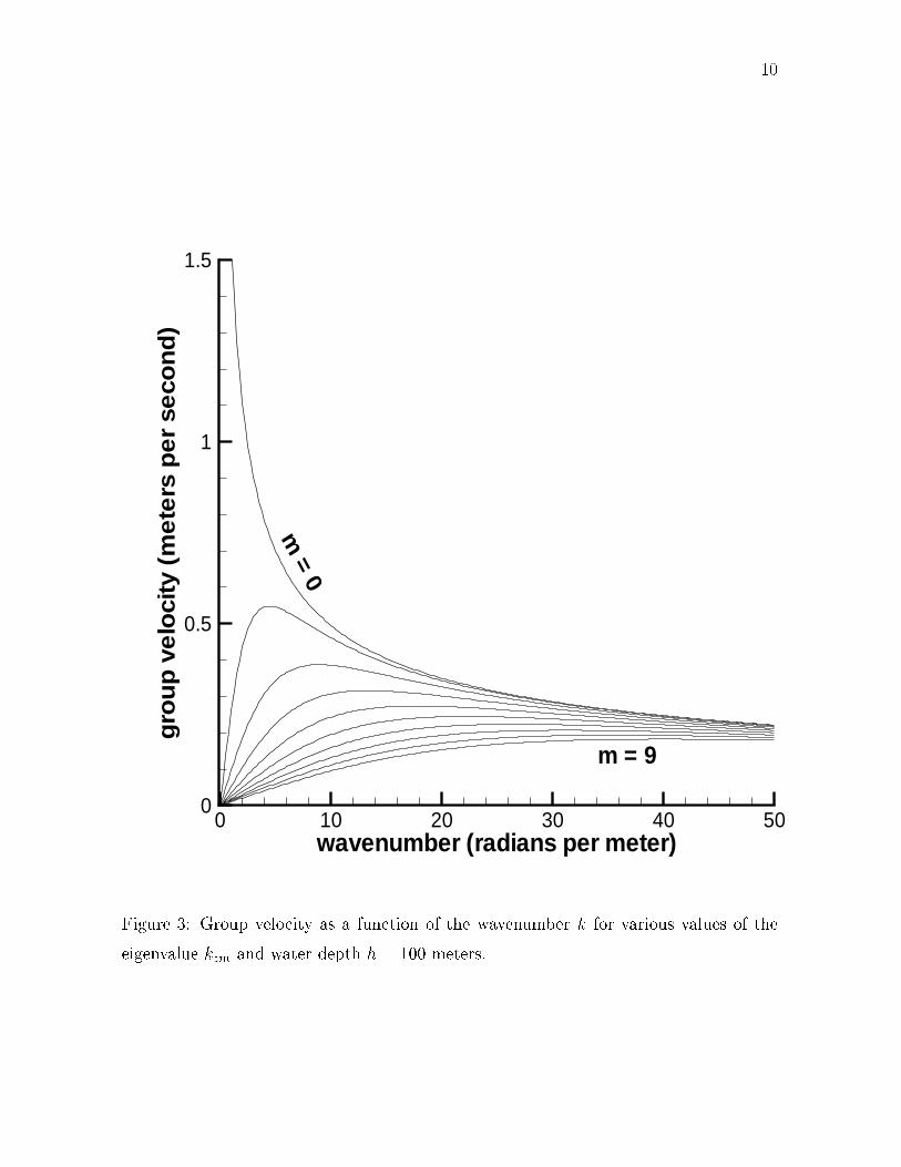
mode group velo ity. In fgures 3 and ., we plot the group velo ity for the frst 10

wave modes asso iated with the eigenvalues kz (m from 0 to 9). For wave frequen ies

above the ut-of frequen y, the onsidered wave mode (fxed value of kz ) has a real

wavenumb e r k and non-zero group velo ity, a s w e an see through fgures 3 and .. As the

wave frequen y approa hes the ut-of frequen y, the group velo ity of the onsidered

wave mode approa hes zero, a ording to fgures 3 and .. At the ut-of frequen y of

the onsidered wave mode, its group velo ity is zero and no energy is transported by

7

wa

ve f

req

ue

ncy

(ra

dia

ns

pe

r se

con

d)

22

20

18

16

14

12

10

8

6

4

2

m = 9

m=

0

0 10 20 30 40 50 wavenumber (radians per meter)

Figure 1: \ave frequen y as a fun tion of the wavenumb e r k for various values of the

eigenvalue kz and water depth h = 100 meters.

8

wa

ve f

req

ue

ncy

(ra

dia

ns

pe

r se

con

d)

24

22

20

18

16

14

12

10

8

6

4

2

m = 9 m

=0

0 10 20 30 40 50 wavenumber (radians per meter)

Figure 2: \ave frequen y as a fun tion of the wavenumb e r k for various values of the

eigenvalue kz and water depth h = 0 .1 meters.

9

this wave mode for wave frequen ies at or b e l o w the wave mode ut-of frequen y.

A ording to fgures 3 and ., the group velo ity f o r e a h w ave mode has a maximum

value, whi h de ays as the value of kz in reases (value of m in reases). The frst wave

mode (sine wave mode with kz

= 0) has the largest maximum group velo ity, and sin e

its ut-of frequen y is zero, we a n h a ve free propagating waves for any w ave frequen y

for the hannel spe ifed by its depth h, its width 2b and the gravity a eleration g.

Above, we l o o k ed at the wave modes with sine dependen e in the z oordinate. For the

wave modes with osine dependen e in the z oordinate, the minimum absolute value

of the eigenvalue kz is larger than the minimum absolute value for the eigenvalues

kz , whi h is zero. Therefore, for any wave frequen y we have free waves propagating

along the hannel. For the osine wave modes there is a minimum ut-of frequen y.

Propagation of this type of wave mode is possible only for wave frequen ies above their

minimum ut-of frequen y.

2 For ed Wave Propagation Along a Narrow Waveg­

uide.

Now we onsider for ed waves propagating along a semi-infnite hannel with the same

depth h and width 2b as the hannel in the previous se tion. The semi-infnite hannel

has a wave maker at one edge of the hannel, whi h generates wave disturban es that

may o r m a y not propagate along the hannel. The solution for the for ed waves is given

as a superposition of wave modes. The same wave modes we obtained in the previous

se tion. Evanes ent wave modes are also part of the solution in this ase. They stay lo-

alized lose to the wave m a k er and des ribe the lo al wave f e l d . For a mono- hromati

ex itation, the wave modes with ut-of frequen y b e l o w the ex itation frequen y on-

stitute the propagating wave feld, and the wave modes with ut-of frequen y above th e

ex itation frequen y are evanes ent and stay lo alized lose to the wave maker. Their

superposition gives the evanes ent wave feld.

10

gro

up

ve

loci

ty (

me

ters

pe

r se

con

d)

0

0.5

1

1.5

m = 9

m=

0

0 10 20 30 40 50 wavenumber (radians per meter)

Figure 3: Group velo ity as a fun tion of the wavenumb e r k for various values of the

eigenvalue kz and water depth h = 100 meters.

11

gro

up

ve

loci

ty (

me

ters

pe

r se

con

d)

0

0.1

0.2

0.3

0.4

0.5

0.6

0.7

0.8

0.9

1

m = 9

m=

0

0 10 20 30 40 50 wavenumber (radians per meter)

Figure .: Group velo ity as a fun tion of the wavenumb e r k for various values of the

eigenvalue kz and water depth h = 0 .1 meters.

12

3 Initial Boundary Value Problem.

\e onsider the same oordinate system used in the previous se tion. The wave maker is

lo ated at x = 0 and the hannel lays at x > 0. The linearized boundary value problem

for the for ed waves is similar to the boundary value problem for the free waves problem.

The diferen e is the boundary ondition des ribing the efe t of the wave maker and

the fa t that the hannel is now semi-infnite. The linear boundary value problem for

for ed waves is given by the set of equations

V2<(x, y, z, t) = 0 for 0 x o, -h y 0 and - b z b, (3.26)

�2< �<

+ g =0 at y = 0 , (3.27)�t

2 �y

�<

=0 at y = -h, (3.28)�y

�<

=0 at z = ±b, (3.29)�z

�< wA

= F (z)G(y)f(t) on x = 0 , (3.30)�x b

and the free surfa e displa ement r(x, z, t) is related to the potential fun tion <(x , y , z, t )

a ording to the equation

1 �<

r(x, z, t) = - (x, 0, z, t ). (3.31)

g � t

The fun tion f(t) is a known fun tion of time. A tually, we hose an harmoni ex ita-

tion, so we have

f(t) = os(wt ), (3.32)

where w is the ex itation frequen y. \e need also to onsider initial onditions for the

boundary value problem above. They are given by the equations

<(x, y, z, 0) =0, (3.33)

<t(x, y, z, 0) =0, (3.3.)

13

where the initial ondition (3.3.) is equivalent to have a still free surfa e at t =

0 (r(x, z, 0) = 0). Next, we solve the initial boundary value problem, whi h is dis-

ussed in the next se tion.

3.1 Solution of the Initial Boundary Value Problem.

The frst step to solve the initial b o u n d a r y value problem given by equations (3.26)

to (3.30) is to apply the osine transform in the x variable. This results in a non-

homogeneous Helmholtz-like equation for the potential fun tion under homogeneous

boundary onditions. Sin e the resulting equation is non-homogeneous, the solution

is given as the superposition of the solution for the homogeneous part of the problem

plus a parti ular solution that handles the non-homogeneity. To solve the asso iated

homogeneous problem, we use the method of separation of variables as in the previ-

ous se tion. The solution of the homogeneous problem is given as a superposition of

modes in the y and z variables. The parti ular solution is obtained using the homo-

geneous solution through the method of variation of the parameters. The onstants of

the homogeneous solution are obtained by applying the boundary onditions to the full

solution (homogeneous plus parti ular solutions). Next, we dis uss in detail the steps

outlined above.

\e onsider the osine transform pair

]f (k) = f (x) o s ( k x )dx (3.35)

0

and 1 ]f (x) = f (k) os(kx )dk. (3.36)2t 0

If we apply the osine transform (3.36) to the se ond partial derivative o f t h e potential

fun tion <(x , y , z, t ) w i t h respe t to the x variable, we have that

<xx

os(kx )dx = -<x(0, y , z, t ) - k2<](k , y , z, t ), (3.37)

0

� �

� �

1.

sin e we assumed that <x

- 0 and < - 0 as x -o . The term <x(0, y , z, t ) is spe ifed

by the boundary ondition at x = 0 and given by equation (3.30). Next, we apply

the osine transform to the initial boundary value problem given by equations (3.26) to

(3.30). This results in the set of equations

<]yy

+ <]zz

- k2<] = <x(0, y , z, t ) =

Aw

F (z)G(y) os(wt ), (3.38)b

]<tt

+ g< y

=0 on y = 0 , (3.39)

]<y

=0 on y = -h, (3..0)

]<z

=0 on z = ±b, (3..1)

with the initial onditions given by equations (3.33) and (3.3.) written in the form

]<(k , y , z, 0) =0, (3..2)

]<t(k , y , z, 0) =0. (3..3)

This is a non-homogeneous initial boundary value problem for the fun tion <](k , y , z, t )

( osine transform of <(x, y, z, t)). Our strategy to solve this initial boundary value

problem is to fnd the general form of the solution of the homogeneous part of the

initial boundary value problem given by equations (3.38) to (3..1) plus a parti ular

solution for the non-homogeneous part of this initial boundary value problem. To fnd

the value of the onstants of the homogeneous part of the solution, we apply the initial

and boundary onditions to the full solution (homogeneous plus parti ular). Next, we

onsider the homogeneous part of the initial b o u n d a r y value problem for <], whi h is

given as the superposition of wave modes obtained in the previous se tion. So, the

solution of the homogeneous problem is similar to the one given by equation (1.2.).

The solution for the homogeneous problem is

]<H

= {[A (k , t ) osh(A (y + h)) + B (k , t ) sinh(A (y + h))] os(kz z)}

+ {[C (k , t ) osh(A (y + h)) + D (k , t ) sinh(A (y + h))] sin(kz z)} ,

� �

� �

� �

� �

15

where A2 = k2 +kz 2 , A2 = k2 +kz

2 , and kz and kz are given respe tively, in equations

(1.16) and (1.15). As we mentioned before, the general solution is given as a superpo-

sition of the homogeneous solution <]H

plus a parti ular solution. \e assume that the

parti ular solution has the form

]{[

D] }

<p

= A (k , y , t ) osh(A (y + h)) +

D k , y , t ) sinh(A (y + h)) os(kzB ( z)

{[D

] }+ C (k , y , t ) osh(A (y + h)) +

DD (k , y , t ) sinh(A (y + h)) sin(kz z) .

\e substitute the potential <]p

in the non-homogeneous Helmholtz equation (3.38) in

the y and z variables. \e also impose that

{ [ ] }�<]p D= A A sinh(A (y + h)) +

D osh(A (y + h)) os(kz z)B

�y

(3...) { [ ] }

+ A CD sinh(A (y + h)) +

DD osh(A (y + h)) sin(kz z) .

The pro edure above results in the set of equations for the amplitudes

D ,

D , CD andA B

DD .

(AD )y

osh(A (y + h)) + (BD )y

sinh(A (y + h)) =0, (3..5)

(CD )y

osh(A (y + h)) + (DD )y

sinh(A (y + h)) =0, (3..6) { } Aw

A (AD )y

sinh(A (y + h)) + (BD )y

osh(A (y + h)) =

b2

G(y) os( wt )F , (3..7) { } Aw

A (CD )y

sinh(A (y + h)) + ( DD )y

osh(A (y + h)) =

b2

G(y) os( wt )F , (3..8)

where

F

F

=

=

:

:

F (z) s i n (kz

:

:

F (z) os(kz

z)dz,

z)dz.

(3..9)

(3.50)

�

�

16

If we solve the set of equations above and integrate with respe t to the y variable

D D Dfrom -h to 0, we obtain the following expressions for the amplitudes A , B , C and

DD , w h i h follows:

AwDA = - os(wt )F G (y), (3.51)b2A

BD =

Aw

os(wt )F H (y), (3.52)b2A

AwDC = - os(wt )F G (y), (3.53)b2A

AwDD = os(wt )F H (y), (3.5.)b2A

where the fun tions G (y), H (y), G (y) and H (y) are given by the equations

y

G (y) = G(p) sinh(A (p + h))dp, (3.55)

:

y

H (y) = G(p) osh(A (p + h))dp, (3.56):

y

G (y) = G(p) sinh(A (p + h))dp, (3.57):

y

H (y) = G(p) osh(A (p + h))dp. (3.58):

Now, the total solution <](k , y , z ) a n written in the form

Aw]< = A - os(wt )F G (y) osh(A (y + h))b2A

Aw

+ B + os(wt )F H (y) sinh(A (y + h)) os(kz z)b2A (3.59)

Aw

+ C - os(wt )F G (y) osh(A (y + h))b2A

Aw

+ D + os(wt )F H (y) sinh(A (y + h)) sin(kz z) .

b2A

In the expression above w e still need to obtain the onstants A , B , C and D of the

homogeneous part of the solution. To do so, we apply the boundary onditions (3.39)

17

at y = 0 and (3..0) at y = -h. The boundary ondition at y = -h, given by the

equation (3..0), implies that D = 0( B = 0). The boundary ondition at y = 0 gives

the equation

(A )tt

+ gA tanh(A h)A =

A

b2

F

A

{w3 os(w t ) [ H (0) tanh(A h) -G (0)]

(3.60)

+gA w os(w t ) [ G (0) tanh(A h) -H (0)]} .

\e also obtain a similar equation for C . This is a non-homogeneous se ond order dif-

ferential equation in time for the amplitude A . Its solution is given as the superposition

of the solution of the homogeneous part of the equation plus a parti ular solution whi h

satisfes the non-homogeneous term in the equation (3.60). The homogeneous solution

is given as

] ](A (t))H

= A os(n t) + B sin(n t) (3.61)

with n2 = gA tanh(A h). \e assume the parti ular solution given in the form

] ](A (t))p

= A(t)p

os(nt) + B(t)p

sin(nt). (3.62)

\e impose that

d

{ }] ](A (t))p

= n -A(t)p

sin(nt) + B(t)p

os(nt) . (3.63)dt

If we substitute the form of the parti ular solution, given by equation (3.62) into the

governing equation (3.61) and take i n to a ount the assumed form for

f (A (t))p

, givenft

by equation (3.63), we obtain for the amplitudes A](t)p

and B](t)p

the expressions

1 1(w, n , h ) os[(n - w)t] os[(n + w)t]]A(t)p

= + , (3.6.)2 n n - w n + w

1 1(w, n , h ) sin[(n - w)t] sin[(n + w)t]]B(t)p

= + , (3.65)2 n n - w n + w

� �

�

�

18

where

A F

{1(w, n , h ) = w

3 [H (0) tanh(A h) -G (0)]b2 A (3.66)

+gA w [G (0) tanh(A h) -H (0)]}

If we substitute these expressions for the amplitudes A](t)p

and B](t)p

in the assumed

form of the parti ular solution, we obtain

1(w, n , h )(A (t))p

= - os(wt ). (3.67)

w2 - n2

As a result, we obtain for A (t) the following expression:

1(w, A, h )] ]A (t) = A os(n t) + B sin(n t) - os(wt ) (3.68)(w2 - n2)

For the amplitude C we obtain the same expression as above for A (t), but with

the index m instead of the index n. Now the potential fun tion an b e written in the

form

1(w, A , h )] ] ]< = A os(n t) + B sin(n t) - os(wt )(w2 - n2)

A F A F

-b2

w os(w t )A

G (y) osh(A (y + h)) +

b2

w os(w t )A

H (y) sinh(A (y + h)) os(kz z)

1(w, A , h )] ]+ C os(n t) + D sin(n t) - os(wt )2 - n2(w )

A F A F

- w os(wt ) G (y) osh(A (y + h)) + w os(wt ) H (y) sinh(A (y + h)) sin(kz z) ,

b2 A b2 A

(3.69)

] ] ] ]whi h is a fun tion of the unknown onstants A , B , C and D . To obtain these

] onstants we use the initial onditions for <(k , y , z, t ) given by equations (3..2) and

(3..3). \e obtain

� �

�

�

19

1(w, A , h ) A wF A wF]A = + G (0) - H (0) tanh(A h), (3.70)

w2 - n2 b2 A b2 A

]B =0, (3.71)

1(w, A , h ) A wF A wF]C = + G (0) - H (0) tanh(A h), (3.72)

w2 - n2 b2 A b2 A

]D =0. (3.73)

The fnal form of the potential fun tion <](k , y , z, t ) is g iv en by the equation

AF w3 os(n t) - os(wt ) osh(A h)]< = - + w ( os(n t) - os(wt ))b2 ,2 (w2 - n2 ) osh(A h) A2

w sinh2(A h) A sinh2(A (y + h))

- os(n t) osh(A (y + h)) + wF os(wt ) os(kz z)A2 osh(A h) b2 A2

AF w3 os(n t) - os(wt ) osh(A h)

+ - + w ( os(n t) - os(wt ))b2 ,2 2 - n2 A2(w ) osh(A h)

w sinh2(A h) A sinh2(A (y + h))

- os(n t) osh(A (y + h)) + wF os(wt ) sin(kz z).

A2 osh(A h) b2 A2

(3.7.)

\e are interested in the displa ement of the free-surfa e r(k , z, t ), whi h is given

in terms of the p o t e n tial fun tion <(k , y , z, t ) a ording to the equation (3.31). Then

the osine transform of the free-surfa e displa ement is given in terms of the Fourier

transform of the potential a ording to the equation

1 �<]r](k , z, t ) = - (x, 0, z, t ). (3.75)

g � t

If we apply this equation to the expression for <](k , y , z, t ) given by equation (3.7.),

we obtain

�

�

�

�

20

AF wn

r](k , z, t ) = (w sin(wt ) - n sin(n t)) os(kz z)2 A2 (w2 - n2 )gb

AF wn

+ (w sin(wt ) - n sin(n t)) os(kz z) .

gb

2 A2 (w2 - n2 )

(3.76)

3.2 Fourier Integral Solution.

Here we apply the inverse osine transform to the expression above for the osine trans-

form of the free-surfa e displa ement. The inverse osine transform is given by equation

(3.36), and we apply it to the equation (3.76) to obtain the free-surfa e displa ement

AF 1 wn

r(x, z, t) = (w sin(wt ) - n sin(n t)) os(kx )dk os(kz z)2 A2 (w2 - n2 )gb 2t 0

AF 1 wn

+ (w sin(wt ) - n sin(n t)) os(kx )dk sin(kz z)2 A2gb 2t 0

(w2 - n2 )

(3.77)

The integrands in the integrals above apparently have p o l e s i n t h e omplex k plane

for wave numbers solutions of w2 - n2 (k) = 0. As n (k) approa hes ±w, we have that

n (k) sin(wt ) approa hes w sin(wt ) in the same fashion, so there is no singularity in

the integrand and the integral is well behaved. To obtain the free-surfa e displa ement

we evaluated numeri ally the inverse osine transforms appearing in equation (3.77).

Results from these simulations were used to generate animations of the evolution of the

free-surfa e displa ement due to the a tion of the wave maker over the fuid. These

animations are dis ussed in the next se tion.

3.3 Numeri al Results.

Here we s h o w results from the numeri al evaluation of the inverse osine transforms ap-

pearing in the equation (3.77) for the free-surfa e displa ement. \e d i s p l a y t h e e v olution

of the free-surfa e displa ement in time through the numeri al evaluation of equation

(3.77). \e generated animations for the evolution of the free-surfa e displa ement due

21

to the a tion of the wave maker at x = 0. Here we dis uss the examples and we give

links for the movies asso iated with these examples.

• \e onsider that the displa ement of the wave maker oin ides with the frst

osine wave mode in the z dire tion. The ex itation frequen y is above the ut-

of frequen y for the frst osine wave mode. \ith this type of ex itation, the

only wave mode taking part in the solution is the frst osine wave mode. Sin e

the wave maker starts from rest to the harmoni motion, it ex ites initially all

wave frequen ies and generates a transient whi h propagates along the hannel

and is followed by a nono- hromati wave train (the osine wave mode) with

frequen y equals to the ex itation frequen y. The transient h a s a w ave f r o n t whi h

propagates with the maximum group velo ity possible for this osine wave mode.

For the depth h = 0 .1 meters, fgure 5 illustrates the maximum group velo ity f o r

the osine wave modes. The maximum group velo ity possible Cg, ax

is the group

;velo ity of the osine wave mode with kz = (n = 0). Then, for a given time

2:

instant t, there is no wave disturban e at positions x > Cg, axt. The transient

for a given instant t stays in the region Cg, axt > x > C g(w)t, where Cg(w) is the

group velo ity of the ex ited osine wave mode at the ex itation frequen y w.

• \e onsider that the displa ement of the wave maker oin ides with the se ond

osine wave mode in the z dire tion. The ex itation frequen y is above t h e ut-of

frequen y for the frst osine mode but below the ut-of frequen y for the se ond

osine mode. Again, the wave maker starts from rest to the harmoni motion.

All wave frequen ies are ex ited initially and a transient develops. The transient

propagates along the hannel, and behind it we are left with only the se ond osine

wave m ode, w hi h de ays exponentially as we go away from the wave m aker, sin e

at this ex itation frequen y the se ond osine wave mode is evanes ent. Again,

the transient has a wave front w h i h propagates with the maximum group velo ity

possible for the se ond osine wave mode.

• \e onsider that the displa ement of the wave maker oin ides with the frst

22

gro

up

ve

loci

ty (

me

ters

pe

r se

con

d)

0.9

0.8

0.7

0.6

0.5

0.4

0.3

0.2

0.1

0 0

Maximum group velocity for 1 st cosine mode

n=

0

n = 9

Maximum group velocity for the 2nd cosine wave mode

10 20 30 40 50 wavenumber (radians per meter)

Figure 5: Group velo ity as a fun tion of the wavenumb e r k for various values of the

eigenvalue kz and water depth h = 0.1 meters. The maximum group velo ity for the

frst osine wave mode (Cg, ax) is indi ated in the fgure. Maximum group velo ity for

the se ond osine mode also indi ated in the fgure.

23

osine mode in the z dire tion. The ex itation frequen y is exa tly at the ut-of

frequen y. Again, the wave maker starts from rest to the harmoni motion, and

initially all wave frequen ies are ex ited. A transient develops and propagates

along the hannel. The transient has a wave front whi h propagates with the

maximum group velo ity possible Cg, ax

for the frst osine wave mode. Behind

the transient w e are left with the frst osine wave mode, sin e it is the only wave

mode ex ited by the wave maker. The group velo ity of this wave mode at its

ut-of frequen y is zero, so there is no energy propagation along the hannel after

the transient part of the solution is already far from the wave maker. Sin e the

energy annot be radiated away from the wave maker, we see the wave amplitude

growing with time lose to the wave maker. The osine wave mode resonates with

the wave maker in this ase.

• Now the wave m a k er is a liner fun tion in the z dire tion (F (z) = z). \e show the

evolution of the disturban e due to the a tion of the wave maker. \e onsider all

modes that take part in the solution. \e a tually onsider only a fnite numb e r

of sine and osine wave modes. As the wavenumb e r kz or kz asso iated with

a wave mode in reases, its amplitude de reases, so only a fnite numb e r of wave

modes are signif ant. Again, the wave maker starts from rest to the harmoni

motion. \e h a ve initially a transient w h i h propagates along the hannel. It has a

wave front whi h propagates with the maximum possible group velo ity, whi h is

the maximum group velo ity for the frst sine wave m o d e . Ahead of the wave front

(x > Cg, axt for a given instant t, where Cg, ax

is the maximum group velo ity

for the frst sine wave mode) we h a ve n o w aves disturban e. For a given instant t,

the transient stays in the region Cg, axt > x > C g(w)t, where Cg(w) is the group

velo ity of the frst sine wave mode at the ex itation frequen y w. Behind this

region we have the steady state solution.

MIT OpenCourseWare https://ocw.mit.edu

2.062J / 1.138J / 18.376J Wave Propagation Spring 2017

For information about citing these materials or our Terms of Use, visit: https://ocw.mit.edu/terms.