Demystifying the Math of the Coronavirus Elon Kohlberg Abraham Neyman

Working Paper 20-112

Working Paper 20-112

Copyright © 2020 by Elon Kohlberg and Abraham Neyman.

Working papers are in draft form. This working paper is distributed for purposes of comment and discussion only. It may not be reproduced without permission of the copyright holder. Copies of working papers are available from the author.

Funding for this research was provided in part by Harvard Business School.

Demystifying the Math of the Coronavirus

Elon Kohlberg Harvard Business School

Abraham Neyman Hebrew University of Jerusalem

Demystifying the Math of the Coronavirus Elon Kohlberg – Harvard Business School

Abraham Neyman – Hebrew University of Jerusalem

Abstract We provide an elementary mathematical description of the spread of the coronavirus. We explain two fundamental relationships: How the rate of growth in new infections is determined by the “effective reproductive number”; and how the effective reproductive number is affected by social distancing. By making a key approximation, we are able to formulate these relationships very simply and thereby avoid complicated mathematics. The same approximation leads to an elementary method for estimating the effective reproductive number. Introduction Our purpose is to provide a simple description of the math underlying the spread of the coronavirus. Obviously, a simple description of such a complex phenomenon cannot be accurate. But we attempt to highlight the main variables and the connections between them. In particular, we explain the meaning of the effective reproductive number, R, and why tracking the value of R is essential for gauging the impact of social distancing. With this in mind, we propose a method for estimating R that, while not as precise as the methods employed by epidemiologists, can be implemented very simply. Our colleagues, Arya Zandvakili and Gavriel Kohlberg, have built a website https://bit.ly/simpleR that exhibits the value of R, calculated this way on a daily basis, in every region of the world. They find close agreement between their estimates and the published values of R. The main variables The first observation is this: Only recently-infected people cause further infections. This is so because after a few days the infected person is identified and isolated, and in any case the period of infectiousness ends when the disease has run its course. This observation leads us to focus not on the total number of infections, but rather on the number of new infections. Specifically, we focus on the daily number of new infections. Since the secondary infections caused by a newly infected person all occur within a short period of time, it is natural to consider them in the aggregate. Thus, we define R: The average number of secondary infections caused by each infected person. This is called the effective reproductive number.

To understand the progression of the virus, we must also consider the time lag between a primary infection and the secondary infections that it causes. Thus, we define D: The average number of days between the moment that someone is infected and the moment that they infect another person. This is called the generation interval. The value of R reflects the intrinsic properties of the virus – mainly, how infectious it is. But R also depends on people’s behavior: absent social distancing, it can be as high as 2 or 3 (it was 2.4 in the early days of the Wuhan epidemic) but with social distancing it is substantially lower. It is important to emphasize that social distancing comprises two elements: Decreasing the number of interactions between infected and uninfected individuals, and reducing the probability of infection in each such interaction. The former is achieved by decreasing the overall number of interactions, by isolating areas that are known to have high rates of infection, and by increasing the frequency of testing and the speed of tracing past contacts of infected people. The latter is achieved by requiring that people wear masks and maintain safe distances. The value of D also reflects the intrinsic properties of the virus – how long it takes for a newly infected person to become infectious to others (the “latent” period) and how long the infectiousness period lasts. Absent social distancing, a newly infected person will infect others throughout the infectiousness period, so that D is roughly equal to the latent period plus one half the infectiousness period. But with testing and contact tracing, the infected person might be identified and isolated much earlier than the end of the infectiousness period. (We discuss this in more detail in the Appendix.) For the coronavirus, we estimate D at about 4 days. This is based on limited available data, e.g., https://www.medrxiv.org/content/10.1101/2020.03.05.20031815v1.full.pdf, and will likely change as more data becomes available. However, such changes will not materially impact the points that we make below. Growth in new infections when R and D are fixed Changes in social distancing bring about changes in R and, to some extent, also changes in D. But in order to have a simple mental model of the progression of the virus, it is useful to first consider the case where R and D are fixed. Imagine then a population where D = 4 days and R = 2.5, and the current rate is 100 daily new infections. On the average, each of these will generate 2.5 additional infections. The 250 additional infections will occur on different dates, some within a couple of days and others a week or two later, but on the average, they will occur 4 days out. To trace how many of them occur on each day is complicated. So, we make a rough approximation and lump them together, assuming that all 250 of them occur on day 4.

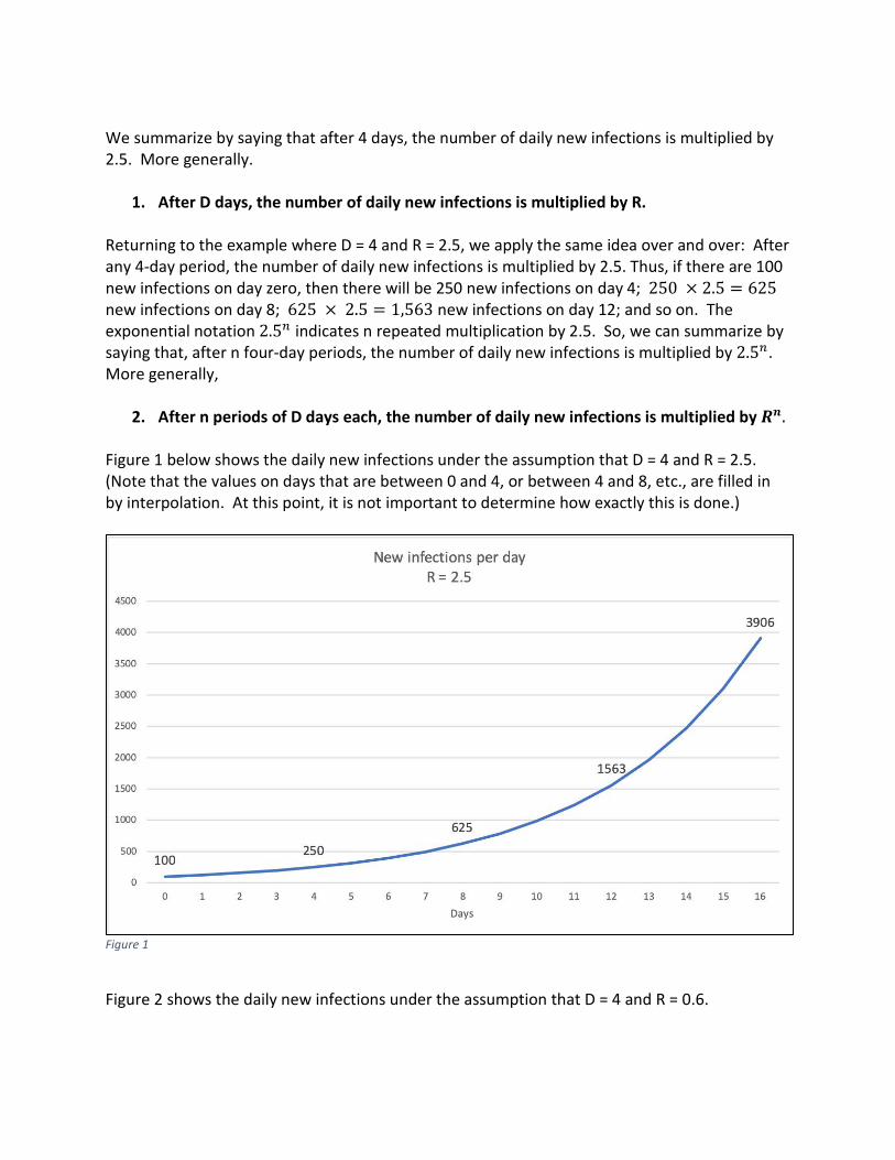
We summarize by saying that after 4 days, the number of daily new infections is multiplied by 2.5. More generally.

1. After D days, the number of daily new infections is multiplied by R. Returning to the example where D = 4 and R = 2.5, we apply the same idea over and over: After any 4-day period, the number of daily new infections is multiplied by 2.5. Thus, if there are 100 new infections on day zero, then there will be 250 new infections on day 4; 250 × 2.5 = 625 new infections on day 8; 625 × 2.5 = 1,563 new infections on day 12; and so on. The exponential notation 2.5𝑛𝑛 indicates n repeated multiplication by 2.5. So, we can summarize by saying that, after n four-day periods, the number of daily new infections is multiplied by 2.5𝑛𝑛. More generally,

2. After n periods of D days each, the number of daily new infections is multiplied by 𝑹𝑹𝒏𝒏.

Figure 1 below shows the daily new infections under the assumption that D = 4 and R = 2.5. (Note that the values on days that are between 0 and 4, or between 4 and 8, etc., are filled in by interpolation. At this point, it is not important to determine how exactly this is done.)

Figure 1

Figure 2 shows the daily new infections under the assumption that D = 4 and R = 0.6.

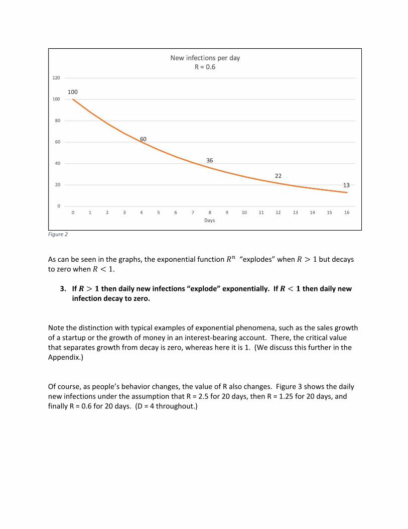
Figure 2

As can be seen in the graphs, the exponential function 𝑅𝑅𝑛𝑛 “explodes” when 𝑅𝑅 > 1 but decays to zero when 𝑅𝑅 < 1.

3. If 𝑹𝑹 > 𝟏𝟏 then daily new infections “explode” exponentially. If 𝑹𝑹 < 𝟏𝟏 then daily new infection decay to zero.

Note the distinction with typical examples of exponential phenomena, such as the sales growth of a startup or the growth of money in an interest-bearing account. There, the critical value that separates growth from decay is zero, whereas here it is 1. (We discuss this further in the Appendix.) Of course, as people’s behavior changes, the value of R also changes. Figure 3 shows the daily new infections under the assumption that R = 2.5 for 20 days, then R = 1.25 for 20 days, and finally R = 0.6 for 20 days. (D = 4 throughout.)

Figure 3 Impact of social distancing Social distancing reduces the number of contacts between people, as well as the probability of infection (“risk”) in each contact. If the number of contacts is reduced by, say, 30% then it stands to reason that R – the average number of new infections generated by each infected person - is also reduced by 30%. Similarly, if the probability of infection in each contact is reduced by 30%, then again R is reduced by 30%. Since every reduction of R by 30% amounts to its reduction to 70% of its previous value, the combined effect reduces R to 70% of 70% of its original value, i.e., R goes down by about 50%. Such a reduction in R has a dramatic effect. For instance, assume the number of daily new infections is 100 and R = 2.5 (and D = 4). If R remains unchanged then 28 days later, daily new infections will explode to about 61,000 (since 2.57 = 610 ). But if R is reduced by 50%, to 1.25, then 28 days later daily new infections will be less than 500 (since 1.257 = 4.8.) The goal of social distancing is to stop the exponential growth of new cases, i.e. to reduce R to 1 and below. To achieve such a reduction, from the current level of R to 1 and below, the multiplicative impact of a reduction in the number of contacts and a reduction in the probability of infection in each contact, must combine to a factor of 1

𝑅𝑅 or less.

100 250 625 15633906

976612190

15216

18993

23708

29594

17747

10643

63833828

2295

0

5000

10000

15000

20000

25000

30000

35000

0 2 4 6 8 10 12 14 16 18 20 22 24 26 28 30 32 34 36 38 40 42 44 46 48 50 52 54 56 58 60

Daily New InfectionsR = 2.5 R = 1.25 R = 0.6

4. Assume R > 1. To stop the exponential growth of new infections, the average number

of contacts must be reduced by some fraction, p, and the riskiness of each contact must be reduced by some fraction, q, in such a way that (𝟏𝟏 − 𝒑𝒑) × (𝟏𝟏 − 𝒒𝒒) ≤ 𝟏𝟏

𝑹𝑹

For example, if R = 2.5 then it is sufficient to reduce the number of contacts by 30% and the probability of infection in each interaction by 50%, since . 7 × .5 = .35 , which is less than 12.5

= .4. If we only reduce one of the variables, say, the number of contacts, then we must have (1 − 𝑝𝑝) ≤ 1

𝑅𝑅 , i.e., 𝑝𝑝 ≤ 1 − 1

𝑅𝑅:

5. To stop the exponential growth of new infections, the average number of contacts

must be reduced by at least the fraction 𝟏𝟏 − 𝟏𝟏𝑹𝑹

(assuming the riskiness of each contact remains the same.)

For example, if R = 2.5, then the number of contacts must be reduced by at least 1 − 1

2.5=

60%. After the epidemic has come under control and social distancing is relaxed, the same considerations indicate how far we can go before R jumps back to 1 and higher.

6. Assume R < 1, and social distancing is relaxed, allowing an increase in the number of contacts by some fraction p and an increase in the riskiness of each contact by some fraction q. To prevent another bout of exponential growth in new infections, p and q must be such that (𝟏𝟏 + 𝒑𝒑) × (𝟏𝟏 + 𝒒𝒒) ≤ 𝟏𝟏

𝑹𝑹.

For example, if R = .7 then it is still safe to increase the number of contacts by 15% and the riskiness of each contact by 15%, since 1.15 × 1.15 = 1.32, which is less than 1

.7= 1.43.

Note: As mentioned above, social distancing impacts not only R but also D. Still, in our approximation we ignore the impact of social distancing on D. This is justified, to some extent, by noting that the main effect of a compression in D is that there are fewer days when the virus is passed on to additional people, but this is captured in the reduction in R.

Herd immunity As the epidemic progresses, we must take into account that not every contact in which the virus is spread to another person constitutes a new infection, for the simple reason that the person might have already been infected. Thus, the number of new infections can be viewed as the product of the number of transmissions of the virus and the fraction of the population that are uninfected. In symbols, 𝑅𝑅 = 𝑅𝑅0 × (1 − 𝐹𝐹), where F is the fraction of the population that are currently infected or immune and 𝑅𝑅0 is the basic reproductive number, defined as follows: R0 - The average number of new infections caused by each infected person, assuming no one else is currently infected. The above formula shows that R may decrease for two reasons: first, stricter social distancing reduces 𝑅𝑅0; second, the progression of the epidemic reduces the fraction (1 – F) of the population that are uninfected. In particular, even when social distancing remains unchanged, the progression of the epidemic will cause R to eventually decline to 1, thereby bringing an end to the exponential growth in new infections. When this occurs, the population is said to have achieved herd immunity. For example, if 𝑅𝑅0 = 2.5 then herd immunity will be achieved when 𝑅𝑅0 × (1 − 𝐹𝐹) = 1, i.e., when F = 60%. More generally,

7. Herd immunity is achieved when the fraction of the population that’s infected or immune is 𝟏𝟏 − 𝟏𝟏

𝑹𝑹𝟎𝟎.

A method for estimating R As we have seen, determining the effective reproductive number, R, and observing how R changes over time, allows us to gauge the impact of social distancing. Epidemiologists employ sophisticated statistical techniques to estimate the value of R from observations about the number of daily infections. To obtain a precise estimate is a difficult challenge. However, if we are willing to accept our basic approximation, that all new infections by an infected individual occur D days after the individual was infected (point #1), as well as the estimate D = 4, then we can write:

𝑁𝑁𝑁𝑁𝑁𝑁 𝑖𝑖𝑖𝑖𝑖𝑖𝑁𝑁𝑖𝑖𝑖𝑖𝑖𝑖𝑖𝑖𝑖𝑖𝑖𝑖 𝑖𝑖𝑖𝑖𝑡𝑡𝑡𝑡𝑡𝑡 = 𝑅𝑅 × 𝑁𝑁𝑁𝑁𝑁𝑁 𝑖𝑖𝑖𝑖𝑖𝑖𝑁𝑁𝑖𝑖𝑖𝑖𝑖𝑖𝑖𝑖𝑖𝑖𝑖𝑖 𝑖𝑖𝑖𝑖𝑓𝑓𝑓𝑓 𝑡𝑡𝑡𝑡𝑡𝑡𝑖𝑖 𝑡𝑡𝑎𝑎𝑖𝑖. Dividing both sides of this equation by “New infections four days ago” gives us an approximation of R:

8. The effective reproductive number can be estimated as follows:

𝑹𝑹𝒆𝒆𝒆𝒆𝒆𝒆 = 𝑵𝑵𝒆𝒆𝑵𝑵 𝒊𝒊𝒏𝒏𝒊𝒊𝒆𝒆𝒊𝒊𝒆𝒆𝒊𝒊𝒊𝒊𝒏𝒏𝒆𝒆 𝒆𝒆𝒊𝒊𝒕𝒕𝒕𝒕𝒕𝒕

𝑵𝑵𝒆𝒆𝑵𝑵 𝒊𝒊𝒏𝒏𝒊𝒊𝒆𝒆𝒊𝒊𝒆𝒆𝒊𝒊𝒊𝒊𝒏𝒏𝒆𝒆 𝟒𝟒 𝒕𝒕𝒕𝒕𝒕𝒕𝒆𝒆 𝒕𝒕𝒂𝒂𝒊𝒊.

Of course, we do not observe the number of all infections but only the number of reported infections. And it is widely recognized that the true number is much greater than the reported number, say by a factor of 5. But for our estimate of R this does not matter: if both numerator and denominator are multiplied by 5, the ratio remains the same. When the frequency of testing increases, then the ratio between the true and the reported numbers declines. But, as long as the frequency of testing changes gradually, then the new (smaller) ratio would be roughly the same today and four days ago, and therefore still cancel in the division. Another difficulty has to do with the fact that the daily numbers of new infections fluctuate for all kinds of random reasons. To smooth out the fluctuations, it might be preferable to use a modified approximation, such as:

𝑅𝑅𝑒𝑒𝑒𝑒𝑒𝑒 = 𝑁𝑁𝑁𝑁𝑁𝑁 𝑖𝑖𝑖𝑖𝑖𝑖𝑁𝑁𝑖𝑖𝑖𝑖𝑖𝑖𝑖𝑖𝑖𝑖𝑖𝑖 𝑖𝑖𝑜𝑜𝑁𝑁𝑓𝑓 𝑖𝑖ℎ𝑁𝑁 𝑙𝑙𝑡𝑡𝑖𝑖𝑖𝑖 4 𝑡𝑡𝑡𝑡𝑡𝑡𝑖𝑖

𝑁𝑁𝑁𝑁𝑁𝑁 𝑖𝑖𝑖𝑖𝑖𝑖𝑁𝑁𝑖𝑖𝑖𝑖𝑖𝑖𝑖𝑖𝑖𝑖𝑖𝑖 𝑖𝑖𝑜𝑜𝑁𝑁𝑓𝑓 𝑖𝑖ℎ𝑁𝑁 𝑝𝑝𝑓𝑓𝑁𝑁𝑜𝑜𝑖𝑖𝑖𝑖𝑓𝑓𝑖𝑖 4 𝑡𝑡𝑡𝑡𝑡𝑡𝑖𝑖.

Given that weekend testing seems to be consistently lower than weekday testing, we might want to modify the approximation even further:

𝑅𝑅𝑒𝑒𝑒𝑒𝑒𝑒 = 𝑁𝑁𝑁𝑁𝑁𝑁 𝑖𝑖𝑖𝑖𝑖𝑖𝑁𝑁𝑖𝑖𝑖𝑖𝑖𝑖𝑖𝑖𝑖𝑖𝑖𝑖 𝑖𝑖𝑜𝑜𝑁𝑁𝑓𝑓 𝑖𝑖ℎ𝑁𝑁 𝑙𝑙𝑡𝑡𝑖𝑖𝑖𝑖 7 𝑡𝑡𝑡𝑡𝑡𝑡𝑖𝑖

𝑁𝑁𝑁𝑁𝑁𝑁 𝑖𝑖𝑖𝑖𝑖𝑖𝑁𝑁𝑖𝑖𝑖𝑖𝑖𝑖𝑖𝑖𝑖𝑖𝑖𝑖 𝑖𝑖𝑜𝑜𝑁𝑁𝑓𝑓 𝑖𝑖ℎ𝑁𝑁 𝑙𝑙𝑡𝑡𝑖𝑖𝑖𝑖 7 𝑡𝑡𝑡𝑡𝑡𝑡𝑖𝑖 𝑖𝑖ℎ𝑖𝑖𝑖𝑖𝑖𝑖𝑁𝑁𝑡𝑡 4 𝑡𝑡𝑡𝑡𝑡𝑡𝑖𝑖 𝑏𝑏𝑡𝑡𝑖𝑖𝑏𝑏.

This estimate of R is not nearly as good as estimates derived from the epidemiological models. But its advantage is that it can be done in real time without requiring anything beyond simple division. This gives people a way to continuously monitor the impact of social distancing in the geographic areas that are of interest to them.

The rate of increase in daily new infection As one follows the progression of the virus, it is natural to focus on the daily growth factor of new infections:

𝑓𝑓 = 𝑁𝑁𝑁𝑁𝑁𝑁 𝑖𝑖𝑖𝑖𝑖𝑖𝑁𝑁𝑖𝑖𝑖𝑖𝑖𝑖𝑖𝑖𝑖𝑖𝑖𝑖 𝑖𝑖𝑖𝑖𝑡𝑡𝑡𝑡𝑡𝑡

𝑁𝑁𝑁𝑁𝑁𝑁 𝑖𝑖𝑖𝑖𝑖𝑖𝑁𝑁𝑖𝑖𝑖𝑖𝑖𝑖𝑖𝑖𝑖𝑖𝑖𝑖 𝑡𝑡𝑁𝑁𝑖𝑖𝑖𝑖𝑁𝑁𝑓𝑓𝑡𝑡𝑡𝑡𝑡𝑡.

If 𝑓𝑓 > 1 then new infections “explode” exponentially, and when 𝑓𝑓 < 1 then new infections decay to zero. But the daily growth factor is not the “right” measure for evaluating the impact of social distancing. This is so because there is no linear relationship between the parameters of social distancing and the daily growth factor. By contrast, there is a linear relationship between the parameters of social distancing and the 4-day growth factor. (More generally, the D-day growth factor.) Indeed, the 4-day growth factor is approximately equal to the effective reproductive number, R (point #2), which is affected linearly by the parameters of social distancing. (See points 4, 5, and 6.) For example, suppose the daily growth factor is 1.2, i.e., new infections are growing by 20% per day. If the average number of contacts between people is reduced by 30%, how will this affect the growth rate of new infections? To answer this question, we first translate r = 1.2 to 𝑅𝑅 = 1.24 = 2.07; next, calculate the change in R: 2.07 × .7 = 1.45; and, finally, translate back to 𝑓𝑓 = 1.45.25 = 1.10. We find that, after the change in social distancing, new infections will grow by 10% per day. To summarize, the unit of time consisting of one day has no special meaning for the progression of the virus, but a unit of D days does. Thus, the natural measure is the D-day growth factor in new infections, R, and not the single day growth factor, r. Summary Our basic approximation is that the number of daily new cases is multiplied by R every D days, where R is the effective reproductive number and D is the generation interval. This approximation yields a simple description of the spread of the virus in terms of these two parameters. The same approximation suggests an elementary method for estimating R from the data on daily new infections.

Keywords: Coronavirus; SARS-CoV-2; COVID-19; Effective reproductive number; Basic reproductive number; Social distancing; Herd immunity.

Appendix How D is determined For a rough mental model of how D is determined, note that it takes about 3 days until the infected person becomes infectious (the latent period) and 2 additional days until the end of the incubation period, when the person becomes symptomatic. Assuming that the person is then immediately isolated, the period where they infect others begins 3 days and ends 5 days after the infection – on the average 4 days later. It is widely recognized that a substantial proportion of all infections are asymptomatic. These people will not be isolated and will therefore continue to infect others throughout the full period of infectiousness, which may last three weeks or even longer. However, as long as there is no widespread testing of asymptomatic people, the asymptomatic infections will not be reported, and so they will not show up in the data. Still, there is an indirect effect, since the time lag between the observation of a primary infection and a subsequent secondary infection may include an intermediate asymptomatic infection that has not been observed. This might explain why some research has found generation intervals that are longer than 4 days. Comparison with compound interest The growth of a population of people infected by the virus is similar but not the same as the growth of money deposited in a bank that pays compound interest. Money generates interest the whole time it’s in the account. By contrast, an infected person generates new infections only for a limited number of days. To put it differently, if we wished to draw on the analogy of exponential growth of money in an interest- paying account, then we’d have to imagine an account that paid interest only on new money, i.e., money that entered the account the previous year. For such an account to grow exponentially the interest rate would have to be greater than 100%. By contrast, a standard account that pays interest on all the money, will grow exponentially as soon as the interest rate was positive.

In symbols, if the interest rate is R then $1 deposited in a standard bank becomes (1 + 𝑅𝑅)𝑛𝑛 dollars after n years; thus, if 𝑅𝑅 > 0 then the money in the account grows exponentially. But $1 deposited in a bank that pays interest only on new money becomes 1 + 𝑅𝑅 + 𝑅𝑅2 + ⋯+ 𝑅𝑅𝑛𝑛 dollars after n years; thus, the money in the account will grow exponentially only if 𝑅𝑅 > 1. (Recall that if 𝑅𝑅 < 1 then 1 + 𝑅𝑅 + 𝑅𝑅2 + ⋯ = 1

1−𝑅𝑅. )

Mathematical summary To understand the progression of the epidemic, we must understand the connection between the growth of new infections and the underlying parameters of the virus. Our approximation (point #2) provides such a connection:

9. If r denotes the growth factor of daily new infections, then

𝑹𝑹 = 𝒓𝒓𝑫𝑫, where R is the effective reproductive number and D the generation time. Thus, if we know R and D, then we can determine the growth factor of new infections:

𝒓𝒓 = 𝑹𝑹𝟏𝟏/𝑫𝑫 For example, assuming D = 4, if R = 2.5 then 𝑓𝑓 = 2.51/4 = 1.26, i.e., daily new infections grow by 26% per day; and if R = 0.6 then r = .88, i.e., daily new infections decrease by 12% per day. In particular, if we know how R and D change over time (as a result of changes in social distancing) then we can determine how the growth rate of new infections will change over time.