2019 Colorado School District Cost of Living Analysis
64
Prepared By: Corona Insights © Corona Insights, 2020 CoronaInsights.com 2019 Colorado School District Cost of Living Analysis Colorado Legislative Council
Transcript of 2019 Colorado School District Cost of Living Analysis

Prepared By: Corona Insights © Corona Insights, 2020 CoronaInsights.com
2019 Colorado School District
Cost of Living Analysis Colorado Legislative Council

CONTENTS
Section 1: Overview of the Study ................................................................................................................ 1
Section 2: 2019 Colorado School District Cost of Living Results ............................................................ 2
Section 3: Methodology ............................................................................................................................ 10
3.1 Identifying the Benchmark Household ....................................................................................................... 10
3.2 Identifying the Market Basket of Goods and Services ............................................................................. 10
3.3 Determining Where, When, and How to Collect Costs of Market Basket Items ................................ 13
3.4 Data Collection Details .................................................................................................................................. 17
3.5 Identifying and Measuring Geographic Shopping Patterns ..................................................................... 26
3.6 Developing Final Cost of Living Measures ................................................................................................ 28
Appendix A: Detailed Results ..................................................................................................................30
Appendix B: Changes from the 2017 Study and Implications ................................................................38
Appendix C: Statistical Measures & Techniques Used in this Report ..................................................42
Appendix D: Raw Pricing Data for Selected Purchase Categories ........................................................46
Appendix E: Shopping Patterns Survey Instrument...............................................................................47
Appendix F: Shopping Patterns Matrices ...............................................................................................48

Page 1
2019 COLORADO SCHOOL DISTRICT
COST OF LIVING ANALYSIS
CONDUCTED FOR THE COLORADO LEGISLATIVE COUNCIL
SECTION 1: OVERVIEW OF THE STUDY
Corona Insights is pleased to present the 2019 Colorado School District Cost of Living Analysis to the
Colorado Legislative Council. The purpose of this study is to create a cost of living index for each of the 178
school districts in Colorado to be utilized in the per pupil funding formula for K-12 education, as mandated by
the Public School Finance Act of 1994.
A cost of living index is a tool for comparing how expensive it is to live in one school district rather than
another. We start by assuming that the same family buys the same things while living in different districts, and
then figure out how much it costs to buy those things if the family is living in district A, how much it costs to
buy those things if they are living in district B, and so on.
For the 2019 Colorado School District Cost of Living Study, our family (i.e., “benchmark household”) is a
family of three people with a total household income of $56,547, which is the average salary of a Colorado
teacher with a bachelor’s degree and 10 or more years of experience.
The research process involves the following steps, which are described in greater detail in Section 3:
1. We assume that the benchmark household spends their money on the same goods and services
that a typical family of that size and income buys according to the national Consumer Expenditure
Survey (CES) conducted by the Bureau of Labor Statistics (BLS).
2. We select a variety of specific items to represent categories of spending. For example, we select a
banana to represent purchases of fruits and vegetables. These items comprise our market basket.
3. Then we collect prices for the items in the market basket from businesses or service providers
(such as a utility) in each district.
4. We ask residents in each school district where they go to shop for retail items in the market basket,
which may be in their own district or in different districts.
5. Based on where people typically shop, and how much items cost in each place, we figure out how
much residents of each district typically pay for the total market basket. This allows us to compare
how expensive it would be for the benchmark family to live in each district.
Section 2 of this report provides the results of this study, with maps and tables showing the relative cost
of living in each school district in Colorado. Section 3 of this report provides in-depth information on the
methodology and methods for the study. Appendices A-F provide additional results, raw data, research
instruments and products, additional documentation on changes from the previous study, and statistical
procedures used.

Page 2
SECTION 2: 2019 COLORADO SCHOOL
DISTRICT COST OF LIVING RESULTS
The table that extends across the following several pages provides the overall cost of living in each of
Colorado’s 178 school districts, as calculated in 2019. Figures are reported in order by District number (and
alphabetically by County name), along with associated rankings, ratings, and comparisons.
Cost of living figures relate to the cost of buying a market basket of goods and services that represents the
spending patterns in the United States of the average 3-person household earning $56,547. (See Section 3.1 for
more discussion of the archetypal household.) More detailed results by expense category may be seen in
Appendix A. Raw data for selected goods may be seen in Appendix D.
The findings are largely consistent with previous years. Aspen continues to have the highest cost of living,
however its disparity is less extreme in 2019 than it was in 2017, largely because of the addition of housing rent
to the market basket, which is discussed in Appendix B. Other mountain resort districts make up the top of
the list, including Summit County, Roaring Fork, Steamboat Springs, and Telluride districts. Boulder remains
near the top at #6, with Denver at #8. The districts with the lowest costs of living are primarily located in the
southeastern corner of the state.

Page 3
Below, two maps provide a visual summary of the cost of living index for the 178 school districts. The first
map is a statewide view and the second is a detailed view of the Denver and Colorado Springs metro areas.
Statewide maps for each major expenditure category are provided in Appendix A.
Note. The index value is the ratio of the cost of the market basket in each district to the statewide average
cost of the market basket. An index value that is greater than 100 means that district is more expensive
than average, while a value less than 100 means that district is less expensive than average. In this map,
shades of green depict less expensive districts, while shades of orange depict more expensive districts.

Page 4
Note. The index value is the ratio of the cost of the market basket in each district to the statewide average
cost of the market basket. An index value that is greater than 100 means that district is more expensive
than average, while a value less than 100 means that district is less expensive than average. In this map,
shades of green depict less expensive districts, while shades of orange depict more expensive districts.

Page 5
2019 Cost of Living Index for Colorado School Districts
School
District
ID County School District Total Index
Rank
2019
State Average $56,547 100
10 Adams MAPLETON 1 $56,774 100 26
20 Adams ADAMS 12 FIVE STAR SCHOOLS $56,884 101 24
30 Adams ADAMS COUNTY 14 $55,792 99 40
40 Adams SCHOOL DISTRICT 27J $56,146 99 32
50 Adams BENNETT 29J $55,562 98 42
60 Adams STRASBURG 31J $55,901 99 36
70 Adams WESTMINSTER PUBLIC SCHOOLS $57,570 102 16
100 Alamosa ALAMOSA RE-11J $51,853 92 120
110 Alamosa SANGRE DE CRISTO RE-22J $52,551 93 105
120 Arapahoe ENGLEWOOD 1 $59,184 105 11
123 Arapahoe SHERIDAN 2 $57,099 101 23
130 Arapahoe CHERRY CREEK 5 $56,689 100 29
140 Arapahoe LITTLETON 6 $58,640 104 13
170 Arapahoe DEER TRAIL 26J $52,865 93 99
180 Arapahoe ADAMS-ARAPAHOE 28J $56,006 99 34
190 Arapahoe BYERS 32J $53,925 95 72
220 Archuleta ARCHULETA COUNTY 50 JT $54,392 96 60
230 Baca WALSH RE-1 $50,699 90 157
240 Baca PRITCHETT RE-3 $49,902 88 169
250 Baca SPRINGFIELD RE-4 $50,460 89 162
260 Baca VILAS RE-5 $50,519 89 160
270 Baca CAMPO RE-6 $50,974 90 151
290 Bent LAS ANIMAS RE-1 $49,152 87 177
310 Bent MC CLAVE RE-2 $51,156 90 146
470 Boulder ST VRAIN VALLEY RE 1J $56,719 100 27
480 Boulder BOULDER VALLEY RE 2 $60,607 107 6
490 Chaffee BUENA VISTA R-31 $56,536 100 30
500 Chaffee SALIDA R-32 $55,669 98 41
510 Cheyenne KIT CARSON R-1 $51,321 91 139
520 Cheyenne CHEYENNE COUNTY RE-5 $51,422 91 134
540 Clear Creek CLEAR CREEK RE-1 $54,979 97 53
550 Conejos NORTH CONEJOS RE-1J $50,617 90 159
560 Conejos SANFORD 6J $49,577 88 172
580 Conejos SOUTH CONEJOS RE-10 $50,463 89 161
640 Costilla CENTENNIAL R-1 $51,002 90 150
740 Costilla SIERRA GRANDE R-30 $51,216 91 142
770 Crowley CROWLEY COUNTY RE-1-J $51,038 90 149
860 Custer CUSTER COUNTY SCHOOL DISTRICT C-1 $53,654 95 78
870 Delta DELTA COUNTY 50(J) $51,797 92 123

Page 6
2019 Cost of Living Index for Colorado School Districts
School
District
ID County School District Total Index
Rank
2019
State Average $56,547 100
880 Denver DENVER COUNTY 1 $60,348 107 8
890 Dolores DOLORES COUNTY RE NO.2 $54,176 96 66
900 Douglas DOUGLAS COUNTY RE 1 $57,377 101 19
910 Eagle EAGLE COUNTY RE 50 $60,522 107 7
920 Elbert ELIZABETH SCHOOL DISTRICT $54,306 96 62
930 Elbert KIOWA C-2 $53,693 95 75
940 Elbert BIG SANDY 100J $50,637 90 158
950 Elbert ELBERT 200 $54,626 97 58
960 Elbert AGATE 300 $52,565 93 104
970 El Paso CALHAN RJ-1 $52,093 92 112
980 El Paso HARRISON 2 $53,682 95 77
990 El Paso WIDEFIELD 3 $55,119 97 49
1000 El Paso FOUNTAIN 8 $54,070 96 67
1010 El Paso COLORADO SPRINGS 11 $54,354 96 61
1020 El Paso CHEYENNE MOUNTAIN 12 $55,100 97 51
1030 El Paso MANITOU SPRINGS 14 $57,726 102 15
1040 El Paso ACADEMY 20 $55,421 98 45
1050 El Paso ELLICOTT 22 $53,107 94 91
1060 El Paso PEYTON 23 JT $52,525 93 106
1070 El Paso HANOVER 28 $53,490 95 86
1080 El Paso LEWIS-PALMER 38 $56,238 99 31
1110 El Paso DISTRICT 49 $54,691 97 57
1120 El Paso EDISON 54 JT $51,983 92 114
1130 El Paso MIAMI/YODER 60 JT $51,933 92 118
1140 Fremont CANON CITY RE-1 $53,027 94 92
1150 Fremont FREMONT RE-2 $52,910 94 95
1160 Fremont COTOPAXI RE-3 $52,874 94 96
1180 Garfield ROARING FORK RE-1 $64,234 114 3
1195 Garfield GARFIELD RE-2 $56,715 100 28
1220 Garfield GARFIELD 16 $52,873 94 98
1330 Gilpin GILPIN COUNTY RE-1 $53,249 94 90
1340 Grand WEST GRAND 1-JT $57,126 101 22
1350 Grand EAST GRAND 2 $59,545 105 9
1360 Gunnison GUNNISON WATERSHED RE1J $59,469 105 10
1380 Hinsdale HINSDALE COUNTY RE 1 $55,945 99 35
1390 Huerfano HUERFANO RE-1 $50,117 89 167
1400 Huerfano LA VETA RE-2 $51,167 90 145
1410 Jackson NORTH PARK R-1 $55,530 98 44

Page 7
2019 Cost of Living Index for Colorado School Districts
School
District
ID County School District Total Index
Rank
2019
State Average $56,547 100
1420 Jefferson JEFFERSON COUNTY R-1 $57,178 101 21
1430 Kiowa EADS RE-1 $51,111 90 148
1440 Kiowa PLAINVIEW RE-2 $50,333 89 165
1450 Kit Carson ARRIBA-FLAGLER C-20 $51,637 91 129
1460 Kit Carson HI-PLAINS R-23 $50,384 89 163
1480 Kit Carson STRATTON R-4 $52,038 92 113
1490 Kit Carson BETHUNE R-5 $52,163 92 109
1500 Kit Carson BURLINGTON RE-6J $53,990 95 71
1510 Lake LAKE COUNTY R-1 $57,436 102 18
1520 La Plata DURANGO 9-R $56,867 101 25
1530 La Plata BAYFIELD 10 JT-R $54,803 97 56
1540 La Plata IGNACIO 11 JT $53,625 95 81
1550 Larimer POUDRE R-1 $55,137 98 48
1560 Larimer THOMPSON R2-J $56,049 99 33
1570 Larimer ESTES PARK R-3 $59,152 105 12
1580 Las Animas TRINIDAD 1 $51,170 90 144
1590 Las Animas PRIMERO REORGANIZED 2 $50,937 90 153
1600 Las Animas HOEHNE REORGANIZED 3 $51,416 91 136
1620 Las Animas AGUILAR REORGANIZED 6 $50,741 90 155
1750 Las Animas BRANSON REORGANIZED 82 $50,002 88 168
1760 Las Animas KIM REORGANIZED 88 $49,577 88 171
1780 Lincoln GENOA-HUGO C113 $51,625 91 131
1790 Lincoln LIMON RE-4J $53,649 95 79
1810 Lincoln KARVAL RE-23 $51,390 91 137
1828 Logan VALLEY RE-1 $53,249 94 89
1850 Logan FRENCHMAN RE-3 $51,951 92 116
1860 Logan BUFFALO RE-4J $52,859 93 100
1870 Logan PLATEAU RE-5 $51,640 91 128
1980 Mesa DE BEQUE 49JT $52,611 93 103
1990 Mesa PLATEAU VALLEY 50 $52,787 93 101
2000 Mesa MESA COUNTY VALLEY 51 $53,690 95 76
2010 Mineral CREEDE SCHOOL DISTRICT $52,941 94 94
2020 Moffat MOFFAT COUNTY RE:NO 1 $54,817 97 55
2035 Montezuma MONTEZUMA-CORTEZ RE-1 $54,484 96 59
2055 Montezuma DOLORES RE-4A $55,110 97 50
2070 Montezuma MANCOS RE-6 $55,554 98 43

Page 8
2019 Cost of Living Index for Colorado School Districts
School
District
ID County School District Total Index
Rank
2019
State Average $56,547 100
2180 Montrose MONTROSE COUNTY RE-1J $53,596 95 83
2190 Montrose WEST END RE-2 $52,432 93 107
2395 Morgan BRUSH RE-2(J) $54,301 96 63
2405 Morgan FORT MORGAN RE-3 $53,737 95 73
2505 Morgan WELDON VALLEY RE-20(J) $53,733 95 74
2515 Morgan WIGGINS RE-50(J) $53,593 95 84
2520 Otero EAST OTERO R-1 $49,317 87 173
2530 Otero ROCKY FORD R-2 $49,198 87 176
2535 Otero MANZANOLA 3J $49,231 87 175
2540 Otero FOWLER R-4J $50,285 89 166
2560 Otero CHERAW 31 $49,281 87 174
2570 Otero SWINK 33 $49,024 87 178
2580 Ouray OURAY R-1 $54,978 97 54
2590 Ouray RIDGWAY R-2 $55,796 99 39
2600 Park PLATTE CANYON 1 $57,227 101 20
2610 Park PARK COUNTY RE-2 $55,274 98 47
2620 Phillips HOLYOKE RE-1J $53,633 95 80
2630 Phillips HAXTUN RE-2J $51,874 92 119
2640 Pitkin ASPEN 1 $73,707 130 1
2650 Prowers GRANADA RE-1 $51,318 91 140
2660 Prowers LAMAR RE-2 $51,468 91 133
2670 Prowers HOLLY RE-3 $51,705 91 126
2680 Prowers WILEY RE-13 JT $51,371 91 138
2690 Pueblo PUEBLO CITY 60 $51,811 92 122
2700 Pueblo PUEBLO COUNTY 70 $52,874 94 97
2710 Rio Blanco MEEKER RE1 $54,019 96 70
2720 Rio Blanco RANGELY RE-4 $51,848 92 121
2730 Rio Grande UPPER RIO GRANDE SCHOOL DISTRICT C-7 $52,135 92 111
2740 Rio Grande MONTE VISTA C-8 $51,171 90 143
2750 Rio Grande SARGENT RE-33J $51,138 90 147
2760 Routt HAYDEN RE-1 $57,454 102 17
2770 Routt STEAMBOAT SPRINGS RE-2 $62,048 110 4
2780 Routt SOUTH ROUTT RE 3 $57,933 102 14
2790 Saguache MOUNTAIN VALLEY RE 1 $50,732 90 156
2800 Saguache MOFFAT 2 $54,048 96 68
2810 Saguache CENTER 26 JT $49,673 88 170

Page 9
2019 Cost of Living Index for Colorado School Districts
School
District
ID County School District Total Index
Rank
2019
State Average $56,547 100
2820 San Juan SILVERTON 1 $55,869 99 38
2830 San Miguel TELLURIDE R-1 $61,962 110 5
2840 San Miguel NORWOOD R-2J $52,966 94 93
2862 Sedgwick JULESBURG RE-1 $50,863 90 154
2865 Sedgwick REVERE SCHOOL DISTRICT $50,367 89 164
3000 Summit SUMMIT RE-1 $64,583 114 2
3010 Teller CRIPPLE CREEK-VICTOR RE-1 $54,199 96 65
3020 Teller WOODLAND PARK RE-2 $55,894 99 37
3030 Washington AKRON R-1 $51,769 92 125
3040 Washington ARICKAREE R-2 $51,627 91 130
3050 Washington OTIS R-3 $52,153 92 110
3060 Washington LONE STAR 101 $51,970 92 115
3070 Washington WOODLIN R-104 $51,935 92 117
3080 Weld WELD COUNTY RE-1 $52,655 93 102
3085 Weld EATON RE-2 $53,284 94 88
3090 Weld WELD COUNTY SCHOOL DISTRICT RE-3J $54,286 96 64
3100 Weld WINDSOR RE-4 $55,380 98 46
3110 Weld JOHNSTOWN-MILLIKEN RE-5J $55,005 97 52
3120 Weld GREELEY 6 $53,602 95 82
3130 Weld PLATTE VALLEY RE-7 $51,641 91 127
3140 Weld WELD RE-8 SCHOOLS $54,042 96 69
3145 Weld AULT-HIGHLAND RE-9 $52,358 93 108
3146 Weld BRIGGSDALE RE-10 $51,417 91 135
3147 Weld PRAIRIE RE-11 $51,288 91 141
3148 Weld PAWNEE RE-12 $50,963 90 152
3200 Yuma YUMA 1 $51,797 92 124
3210 Yuma WRAY RD-2 $53,521 95 85
3220 Yuma IDALIA RJ-3 $53,337 94 87
3230 Yuma LIBERTY J-4 $51,550 91 132

Page 10
SECTION 3: METHODOLOGY
3.1 IDENTIFYING THE BENCHMARK HOUSEHOLD
The first step in a cost of living study is to determine whose cost of living the index will reflect. This entity
is referred to as the “benchmark household”. The 2019 benchmark household was defined by the Colorado
Legislative Council to be a three-person household with a total annual household income of $56,547, which is
the average salary in 2018 of a Colorado teacher with a bachelor’s degree and 10 or more years of experience.
A three-person household is the average household size in Colorado (US Census Bureau, 2014-2018). This
benchmark household was defined in the same way as in prior studies in 2015 and 2017. (Prior to 2015, the
benchmark household was defined using the average teacher salary, overall, without specifying a level of
education and experience.)
Over the past studies, the household size has remained constant, and the household income has increased
at a moderate rate. The table below summarizes the history of benchmark household income values used for
the study.
a Since 2015, the household income definition has specified the
average salary of a Colorado teacher with a bachelor's degree
and 10 or more years of experience. b The 2013 salary was
revised to be consistent with the 2015 household income
definition. The 2013 study originally used a salary of $49,100.
3.2 IDENTIFYING THE MARKET BASKET OF GOODS AND
SERVICES
The next step in a cost of living study is to determine what the benchmark household will buy. The goal of
this step is to develop a list of goods and services that, in combination, can represent the full range of typical
annual purchases for the benchmark household. To begin, we obtain a list of spending categories from the
Year Household Income Percent Change
2019 $56,547 6.5%
2017 $53,115 2.3%
2015a
$51,930 5.3%
2013b
$49,300 0.2%
2011 $49,200 3.6%
2009 $47,500 6.7%
2007 $44,500 3.5%
2005 $43,000 7.5%
2003 $40,000 5.3%
2001 $38,000
Household Income Definition
for 3-Person Benchmark Household

Page 11
Consumer Expenditure Survey (CES), which is conducted by the Bureau of Labor Statistics (BLS). The CES
gathers information on the buying habits of American consumer households and then provides summary data
about what households spend their money on and how much of their spending goes to each category. In
particular, they provide data on the spending habits of 3-person households at different income levels that we
use to calculate typical expenditures for our benchmark family earning $56,547. The table below shows the
major expenditure categories and the amount of income spent on each category, sorted from largest to smallest
expenditures.
Starting from the detailed expenditure categories (provided in the table below), Corona Insights and the
Colorado Legislative Council developed a list of specific goods and services to represent the expenditures of
our benchmark household. This list of goods and services comprise the “market basket” for the cost of living
study. An effort was made to retain market basket items from the previous study, while selecting items to meet
the criteria of a) representativeness of the expenditure category, b) widely available statewide in a substantially
similar form, c) represent a minimum proportion of spending (e.g., at least 0.5%), and d) have prices that vary
more between districts than within districts. More information on the selection criteria for 2019 can be found
in Appendix B.
Expenditure Category
% of Income
2019
% of Income
2017
Housing 32.3% 32.8%
Transportation 16.9% 17.8%
Food 13.5% 13.1%
Healthcare 8.9% 8.3%
Personal taxes 5.2% 4.9%
Entertainment 4.1% 3.8%
Apparel and services 2.7% 3.0%
Personal care products and services 1.2% 1.1%
Tobacco 0.9% 1.0%
Alcoholic beverages 0.5% 0.6%
Other 13.8% 14.2%
Total 100% 100%
Consumer Expenditures for a
3-Person Household Earning $56,547

Page 12
Expenditure Category % of Income Representative Market Basket Items 2019
Food 13.55%
Food at home 8.03%
Cereals and bakery products 1.11% Cheerios
Meats, poultry, fish, and eggs 1.75% Ground Beef
Dairy products 0.79% Milk
Fruits and vegetables 1.54% Bananas
Other food at home 2.84% Coke
Food away from home 5.52% Pizza
Housing 32.31%
Owned Dwellings 10.11%
Mortgage interest and charges 5.14% Mortgage Payment
Property taxes 2.80% Property Taxes
Maintenance, repairs, insurance, other expenses 2.17% Homeowner's Insurance
Rented Dwellings 7.76% Rent Payment
Utilities, fuels, and public services 7.69%
Natural gas 0.69% Natural Gas
Electricity 3.05% Electric
Telephone services 2.81% Telephone
Water and other public services 1.14% Water & Sewer
Household operations 2.45% Day Care Services
Household furnishings and equipment & Housekeeping supplies 4.30% Smoke Detector
Transportation 16.94%
Vehicle purchases (net outlay) & vehicle finance charges 8.05%
Car Payment (Interest rate, bank financing fees,
taxes, title, registration)
Gasoline and motor oil 4.11% Gasoline: 85 Unleaded
Other vehicle expenses 4.78%
Maintenance and repairs 2.02% Oil and Filter Change, Front-End Alignment
Vehicle insurance 2.77% Insurance Premiums
Healthcare 8.92% Health Insurance Premium
Entertainment 4.09% Movie Ticket (First Run, Full Length Film)
Personal care products and services 1.16% Woman's Haircut, Man's Haircut
Personal taxes (not including stimulus) 5.16%
Income Tax with Itemized Deductions for
Mortgage Interest
Other [assumed not to vary between districts] 17.87%
Alcoholic beverages 0.53%
Apparel and services 2.70%
Reading 0.14%
Education 1.14%
Tobacco products and smoking supplies 0.88%
Miscellaneous 1.84%
Cash contributions 2.16%
Personal insurance and pensions 8.50%
Total 100.00%
Consumer Expenditure Survey Categories and Specific Weights Utilized in Cost of Living Index

Page 13
3.3 DETERMINING WHERE, WHEN, AND HOW TO COLLECT
COSTS OF MARKET BASKET ITEMS
Market basket items can be divided into two main categories for data collection. In the first category are
retail goods and services that can be purchased from many shopping locations throughout the state. These
items include groceries, restaurant meals, household items, auto services, gasoline, haircuts, and movies. In the
second category are items most people think of as bills: mortgage and rent payments, car payment, insurance,
utilities, and taxes. In 2019, prices for most of the retail goods and services were obtained by making telephone
calls to individual businesses as well as visits to select websites of retailers. In contrast, prices for most of the
bills were calculated from information provided in government publications, other publicly available data, and
through municipal authorities (either via telephone calls or online, where published).
RETAIL ITEMS
The table below provides the data source and data collection method for each of the retail items.
Market Basket
ItemData Source
Collection
Method
Cereals and bakery
productsCheerios
Fruits and vegetables Bananas
Meats, poultry, fish and
eggsGround beef
Dairy Milk
Other food at home Coke
Food away from home PizzaSample from D&B Hoovers business listings for
Pizza Restaurants
Ho
usin
g
Housekeeping supplies,
furnishings, & equipmentSmoke detector
Sample from D&B Hoovers business listings for
Hardware/Department Stores/Grocery/General
Stores/Drugstores
Entertainment Movie ticketSample from D&B Hoovers business listings for
Movie Theaters
Personal care Man's haircut
Personal care Woman's haircut
Maintenance and repairsOil and filter
change
Maintenance and repairsFront-end
alignment
Gasoline and motor oilGasoline:
85 unleadedOil Price Information Service
Purchase
database
CES Category
Fo
od
Sample from D&B Hoovers business listings for
Grocery/General Stores/Convenience Stores
Phone calls to
businesses
Sample from D&B Hoovers business listings for
Beauty & Barber Shops
Tra
nsp
ort
ati
on
Sample from D&B Hoovers business listings for
Auto Repair

Page 14
For each of the retail items, we identified a set of Standard Industrial Classification (SIC) codes that
corresponded to businesses that were likely to sell the item. We then purchased a list of all businesses associated
with those SIC codes from D&B Hoovers. To select a sample of businesses to collect prices from, we first used
ArcGIS software to map the latitude and longitude coordinates for each business to the school district for each
business using school district shape files available from the Census Bureau. As in the previous study, we
determined that a sample of 10 businesses per item per school district was the minimum target. Because not all
businesses would answer their phones or provide pricing information, we determined to start with a sample of
15 businesses per item per district in order to obtain 10 prices. In many districts, there were fewer than 15
businesses available for some items. In those cases, all known businesses in those districts were included in the
sample. In districts with more than 15 businesses available, a weighted random sample of businesses was
selected where weights were used to ensure that the sample of businesses reflects the market share of businesses
in the community.
From a statistical perspective, if all stores selling a given product had an equal market share, meaning people
were just as likely to buy the product at any store as any other store, then taking a simple random sample of
stores would be appropriate, and calculating simple averages of the prices available at those stores would give
a reasonably accurate measure of what people pay and how confident we are in that estimate as a function of
the sample size within the universe of stores. However, because people tend to shop more at some stores than
others (or more people shop at some stores than others), the average amount paid isn’t a simple average of the
prices available across stores, but is a weighted average of prices available by how many people buy at each
location (i.e., the market share of the location). Rather than weighting the prices obtained on the back end, we
instead sampled businesses according to market share in order to account for this complexity. However, this
methodology was most flawed in small districts where we were likely to gather prices from all businesses selling
a product and weight them equally in calculating a district price, even though there may be one particular
business in that district that is responsible for a disproportionate percentage of sales of that item in that district.
To gather data from the sample of businesses selected, we primarily made phone calls to the individual
businesses, however we also gathered some pricing online, where pricing for individual business locations was
available. In addition, online sources were used to verify business addresses, search for missing or alternate
phone numbers, verify business closures, and search for additional businesses in districts where no businesses
existed in the sample. Online sources were also used if businesses in the district did not provide pricing.
To execute the phone survey, Corona recruited temporary contractors to perform the data collection. A
Corona principal who has been involved in past data collection for this project served as the phone research
manager and was in charge of training and overseeing the staff. All hires were screened, interviewed, and
background checked prior to employment by our staffing agency. Data collectors were paid hourly. Phone calls
and online searches were made from Corona’s office.
Corona developed an overview and training guide for data collectors. Corona then conducted training with
all data collectors. Training time focused on the importance of collecting data in the exact same manner from
all businesses contacted and included how to record prices and how to enter data. Data collectors focused on
one product at a time and prior to starting data collection for a specific item, a thorough review of that market
basket item, including relevant details, common questions and allowed substitutions, was provided. The
research manager and other Corona staff were available for questions during the entire data collection period.
The research manager also made periodic check-ins with the data collectors to answer questions and monitor
progress. Data was entered directly into an Excel spreadsheet.
Most of the phone data collection was completed in a two-week period to minimize variability in pricing
due to timing. The research manager conducted random data checks to ensure the correct prices were collected.

Page 15
Gasoline prices were the only retail item collected in a different manner. The Oil Price Information Service
gathers and compiles daily data on gas prices from individual locations across Colorado and makes this
information available for purchase.
NON-RETAIL ITEMS (“BILLS”)
The table below provides the data source and data collection method for each of the non-retail items.
Data collection for non-retail items was tailored to each item, but in most cases involved locating some
publicly available information and supplementing with phone calls to specific providers or municipal authorities
to fill in missing information. Corona staff executed the data collection for these items, with the exception of
bank rates and fees for the vehicle payment calculation, which were collected by phone calls to banks and credit
Specific Item Data SourceCollection
Method
ShelterMortgage
Payment
Housing values from outside consultant;
interest rate from Zillow
Secondary Data &
Online Sources
Shelter Property TaxesColorado Dept of Local Affairs 2018 Annual
Report and April 2019 Final Residential Rate Study Available online
ShelterHomeowners’
Insurance
Colorado Dept of Regulatory Agencies, Division
of InsuranceAvailable online
Shelter Rent Payment2013 - 2017 American Community Survey (ACS) 5-
year datasetAvailable online
Utilities Electric
Colorado Association of Municipal Utilities, U.S.
Dept of Homeland Secruity, National Oceanic and
Atmospheric Administration, Colorado Public
Utilities Commission
Online sources
Phone calls to
providers
Utilities Natural gas
Colorado Public Utilities Commission, National
Oceanic and Atmospheric Administration, U.S.
Energy Information Administration
Online sources
Phone calls to
providers
Utilities TelephoneColorado Dept of Revenue, Colorado Dept of
Regulatory Agencies,The Tax FoundationAvailable online
UtilitiesWater and
Wastewater
Water and wastewater utilities throughout the state.
Homeguide.com and Homeadvisor.com.
Online sources
Phone calls to
providers
Household
OperationsDay Care Services
The Self-Sufficiency Standard for Colorado 2018;
US Office of Child CareAvailable online
Vehicle purchases &
vehicle finance chargesVehicle Payment
D&B Hoovers business list for banks and credit
unions; Kelley Blue Book; Colorado Dept of
Revenue; Colorado Legislative Council
Available online
(vehicle specs,
taxes, registration)
Phone calls (loan
rates, bank fees)
Vehicle insuranceAuto Insurance
Premium
Colorado Dept of Regulatory Agencies, Division
of Insurance (Plan 2, Driver C)Available online
HealthcareHealth Insurance
Premium
Colorado Dept of Regulatory Agencies, Division
of InsuranceAvailable online
Tra
nsp
ort
ati
on
CES Category
Ho
usin
g

Page 16
unions by the temporary staff, as described in the previous section on phone calls for retail items. More
information about the data collection for each of these items is provided in the next section of the report.

Page 17
3.4 DATA COLLECTION DETAILS
PROCESS OVERVIEW
For the retail items identified above, the data collection process followed the same steps, so we describe
those as a group, below. For each of the non-retail items, we describe their data collection process individually.
RETAIL ITEMS
Retail item prices were collected by telephone for every district. The sample for telephone calls was
prepared following the protocol described in the previous section of the report. Detailed item descriptions for
each of these items, as well as the number of prices obtained for each item is provided in the table below.
After all data was collected, Corona staff validated and cleaned the data. Data collectors included notes
next to any price where the item diverged from the market basket description. We reviewed those notes and
Gather DataValidation &
CleaningOutliers &
InterpolationAdd Taxes
Compute Average Price
for District
Market Basket
ItemDescription
Collection
Method
N Obs
2019
Cereals and bakery
productsCheerios
Price of General Mills Cheerios Toasted Whole Grain Oat Cereal plain,
8.9 oz. If size not available, note difference in size and record price.441
Fruits and vegetables BananasPrice per pound. If bananas are priced by the bag or by the banana, note
that in the file. Do not price organic.350
Meats, poultry, fish and
eggsGround beef
Price per pound of prepackaged, regular ground beef, 80% lean or most
comparable, from a 1 to 2 pound package of loose ground beef. Note 344
Dairy MilkPrice for one gallon (128 Fl. oz.) 2% milk, collect cheapest price. If no
2%, then price (in order of preference) 1%, skim, whole. Note if not 561
Other food at home CokePrice for a 2L bottle of regular Coca-Cola. Do not price diet, caffeine
free, cherry, or other varieties.537
Food away from home PizzaPrice for a cheese pizza, regular or thin crust, 14” diameter (note size if
other).367
Ho
usin
g
Housekeeping supplies,
furnishings, & equipmentSmoke detector
Price of most basic smoke detector offered. Preferably no dual carbon
monoxide, dual sensor, 10 year, or similar. Note any premium features
on model priced.
233
Entertainment Movie ticket Price of adult admission to a first-run, full-length movie. 72
Personal care Man's haircut Price of man's wash, cut, and dry. 476
Personal care Woman's haircut Price of woman's wash, cut, and dry without styling. 451
Maintenance and repairsOil and filter
change
Price of an oil and filter change for a 2015 Ford F150 pickup with a 3.5
liter engine. Price includes new filter, 6 qts of 5w-30 synthetic oil, and
disposal of old oil. Do not price with tax.
334
Maintenance and repairsFront-end
alignment
Price of front-end alignment for a 2015 Ford F150 pickup with 2-wheel
drive.182
Gasoline and motor oilGasoline:
85 unleadedPrice per gallon of self-serve, 85 Octane, unleaded gasoline.
Purchase
database1801
CES Category
Fo
od
Phone calls to
businesses
Tra
nsp
ort
ati
on

Page 18
adjusted any prices accordingly (typically scaling prices for differently sized items or multi-packs) and scanned
for any obvious data entry errors. Next, outliers were identified and removed, using the same rule as the
previous study. Specifically, we used box and whisker plots and truncated extreme values to the boxplot whisker
(i.e., the 25th or 75th percentile plus 1.5 times the inter-quartile range).
Finally, appropriate taxes for each item in each location were added to each price, and an average price was
calculated for each district. For food at home items, appropriate grocery taxes were applied; for food away from
home items, appropriate dining out taxes were applied; and normal sales taxes were applied to the smoke
detector as well as 40% of the oil change price (which reflects the portion of the cost covering materials as
opposed to labor). No tax was applied to haircut prices or front-end alignment prices as they are not considered
taxable goods. Movie ticket prices are taxed in some districts, and taxes were collected with the price where
applicable.
NON-RETAIL ITEMS SUMMARY
Detailed item descriptions for each of the non-retail items, as well as the number of prices obtained for
each item is provided in the table below.
Specific Item DescriptionCollection
Method
N Obs
2019
ShelterMortgage
Payment
Mortgage payment, including principal and interest, based on housing
values provided by outside consultant
Secondary Data &
Online Sources1 per district
Shelter Property TaxesProperty taxes based on district home value, residential assessment rate,
and mill leviesAvailable online
1 per district,
1 per county
ShelterHomeowners’
Insurance
$200,000 frame dwelling, $160,000 contents coverage, $100,000 personal
liability, $1,000 medical expense, $500 deductibleAvailable online
15 providers
in 24 cities
Shelter Rent Payment Median gross rent paid for a three-bedroom home Available onlineEstimates for
159 districts
Utilities ElectricPrice for 700 kWh per month, adjusted for ue by climate, plus utility sales
tax
Online sources
Phone calls to
providers
55 electric
utilities
Utilities Natural gasPrice for 62.5 therm per month, adjusted for use by climate, plus utility
sales tax
Online sources
Phone calls to
providers
68 service
areas
Utilities Telephone Taxes, surcharges, and fees associated with monthly mobile phone service Available onlineNot
applicable
UtilitiesWater and
Wastewater
Annual average bill for water service using 11,000 gallons per month and
wastewater service using 5,000 gallons per month. Well and septic
systems were priced based on item cost and installation, operation, and
maintenance divided by the life expectancy of a system.
Online sources
Phone calls to
providers
276 utilities
Household
OperationsDay Care Services Weekly cost of child day care Available online 3 per county
Vehicle purchases
& vehicle finance
charges
Vehicle Payment
Payment calculated using Blue Book purchase value and interest rate on
loan for full purchase price and bank charges, taxes and registration fees
for 2017 Honda Civic for four years. (2017 Honda Civic LX Sedan, 4-
door. Engine: 4-cyl. 2.0L. Trans: Automatic/CVT. Mileage: 24,000.
Amenities: air conditioning, pwr. steering, cruise control, air bags - front
& side, stability control/traction control).
Available online
(vehicle specs,
taxes, registration)
Phone calls (loan
rates, bank fees)
290 banks/
credit unions
Vehicle insuranceAuto Insurance
Premium
Insurance premiums for 2017 Ford Fusion SE 2.5L Automatic with
liability policy limits of $25,000/$50,000/$100,000, $50,000/$100,000
uninsured motorist coverage and with a $500 deductible. For a 35-yr old
male driver, married, principal operator, drives less than 15 miles to work
each way, no accidents or traffic convictions in three years.
Available online16 providers
in 24 cities
HealthcareHealth Insurance
Premium
Prices of health care insurance premiums for a 40-year old. Average price
of "Bronze" and "Silver" health insurance premiums.Available online
2 to 6 per
MSA
Tra
nsp
ort
ati
on
CES Category
Ho
usin
g

Page 19
HOUSING – SHELTER – MORTGAGE PAYMENT/PROPERTY TAXES
Home values were provided to Corona Insights by the Colorado Legislative Council via a study by an
outside consultant, and they were based on a specified home size. This is the same approach used in previous
years. Corona Insights calculated an annual mortgage payment (principal and interest) based on a 30-year fixed
rate mortgage for 80 percent of the home value with the current mortgage interest rate for Colorado on the day
the home values were delivered to Corona Insights.
Owners of residential homes are subject to property tax on their dwelling. The entire value of the home is
not taxed; only the assessed value of the home can be taxed. The assessed value of a home is the actual home
value multiplied by an assessment percentage. This assessment percentage is the same for the entire state of
Colorado and is 7.15% for 2019. The assessed value of the home is then multiplied by the decimal equivalent
of the total mill levy. The total mill levy is the sum of the mill levies from the county, city, school district, and
any other special levies an area may have. To get the decimal equivalent of a mill levy, the levy is multiplied by
.001.
Mill levies were obtained from the 2018 annual report for the Department of Local Affairs. This report
was the most recent report available from the Division of Property Taxation. The report included mill levies
for every county, city, school district, and any other applicable levy in the state of Colorado. The mill levies
were summed by school district. The stated home price for each school district was multiplied by the assessment
percentage to get the assessed value. The assessed value was multiplied by the total of all applicable mill levies
for the district (county, school district, average municipal value in the county, and any special levy) to calculate
the property tax. This process was repeated for all school districts.
HOUSING – SHELTER – HOMEOWNER’S INSURANCE
Homeowner insurance rates were collected from the most recent Homeowners Insurance Premiums
Report provided to Corona by the Colorado Department of Regulatory Agencies, Division of Insurance. Rates
in this report were drawn from a survey of insurance providers that the Division of Insurance conducts
annually; data in the report was current as of July 2018. Premiums were for a coverage period of one year and
were based on full replacement cost coverage. Premiums were calculated based on a HO-3 policy, which is the
most commonly written policy for a homeowner. The HO-3 policy assumed the home was frame structure, 10
years old, equipped with dead-bolt locks and smoke detectors, was within 5 miles of a fire station, and was
within 1,000 feet of a fire hydrant. The policy limits were based on a dwelling replacement cost of $200,000, a
contents replacement of $160,000, personal liability of $100,000, medical expense of $1,000 and a $500
deductible. These specifications were also used in the 2017 and 2015 studies.
The Homeowners Insurance Premiums Report included premiums in 24 cities spread throughout Colorado
from 64 insurance companies. To better represent “typical” homeowner insurance rates, Corona excluded
insurance companies that made up less than one percent of the Direct Written Premium market share in
Colorado. Thus, our analysis included premiums from the 15 largest homeowner insurance providers, which in
aggregate, make up 77 percent of the Colorado homeowner insurance market. We averaged the premiums from
these 15 insurance providers for each of the 24 Colorado cities in the report. Lastly, to derive homeowner
insurance premiums for each school district, Corona predicted premium rates in districts that were not already
represented in the insurance data, based on spatial patterns of the 24 cities from which we did have data. This
interpolation method was also employed to predict homeowner insurance rates in the 2017 and 2015 studies.

Page 20
HOUSING – SHELTER – RENT
Home rental costs were primarily based on median gross rent estimates for a 3-bedroom home by school
districts. The data source was the U.S. Census Bureau’s 2013-2017 American Community Survey (ACS) 5-year
estimates (e.g., table B25031). The universe was all renter-occupied housing units paying cash rent. This dataset
provided rent estimates for 159 of the 178 school districts. However, the margin of error of the median gross
rent estimate was relatively large (i.e., margin of error was either larger than $140 or was greater than 20 percent
of the estimate) for 59 of the 159 school districts. In some of these districts, the margin of error for the median
rent of a 2-bedroom unit was acceptable (i.e., margin of error was either less than $130 or was less than 20
percent of the estimate). In these districts, we inflated the rate of the 2-bedroom estimate by the average percent
difference between 2-bedroom and 3 bedroom medians estimates (among districts with margins of error below
15 percent of the estimate for both the 2- and 3-bedroom estimates) within its region (regions were classified
as school districts in the Easter Plains, Front Range, Mountain Resort Communities, or Non-resort
Communities). In three cases, we decided using the 3-bedroom estimate was more appropriate than inflating
the 2-bedroom estimate, even when the 3-bedroom estimate had a relatively large margin of error.
Using this approach, we estimated median gross rent for 24 districts and relied on the ACS estimate for
100 districts. This left 54 districts without rent values. To calculate the cost to rent for these remaining districts,
we used an interpolation technique, which predicted rental costs based on spatial patterns within the districts
for which we had rent estimates.
Next, we added renter’s insurance costs for each school district. Akin to collecting and calculating
homeowner insurance premiums as described above, Corona collected renter’s insurance policy premiums
provided to Corona by the Colorado Department of Regulatory Agencies, Division of Insurance. Premiums
were calculated for a HO-4 policy, which assumed the home was a frame structure. The policy limits included
contents replacement cost of $40,000, personal liability of $100,000, medical expense of $1,000 and a $500
deductible. Finally, to derive homeowner insurance premiums for each school district, Corona used a spatial
interpolation technique to predict premium rates in districts that were not yet represented, based on spatial
patterns of premium rates among the 24 cities provided by the Division of Insurance.
HOUSING – UTILITIES – ELECTRIC
To estimate an average monthly electric bill within each school district, Corona calculated standardized
electric rates by provider, allocated those rates to census blocks in each provider’s service area, adjusted electric
use based on local climate, applied location specific utility taxes, and then calculated an average electric bill
within each school district. Specific details follow.
Electric utility rates were collected from the most recent survey of electric utility providers, which was
conducted by the Colorado Association of Municipal Utilities (CAMU). CAMU collected billing rates, based
on 700-megawatt usage, from Colorado electric utilities in July 2018 and July 2019. These rates include tax
equivalents, either the exact PILOT (payment in lieu of taxes) or transfer to the municipal general fund, but did
not include county or municipal sales tax. We used the most recent rate available for each utility. The CAMU
dataset did not include rates from the towns of Center, Holyoke, Yuma, or Haxtun, so Corona collected these
rates by calling the municipal utilities.
Next, Corona retrieved the Electric Retail Service Territories global information system (GIS) shapefile
from the United States Department of Homeland Security, Homeland Infrastructure Foundation – Level Data
(HIFLD). We appended the CAMU electric rates to each electric provider.

Page 21
The 2013 cost of living study acknowledged that electricity usage likely varies across geographies based on
climate. For example, households in Southeast Colorado, where summer temperatures are typically much higher
than elsewhere in the state, likely use more electricity for home cooling. In this study, Corona accounted for
this disproportionate use by applying an upward adjustment factor for households in counties where the average
June to September temperature was higher than the average statewide June to September temperature, as
reported by the National Oceanic and Atmospheric Administration, National Centers for Environmental
Information. For example, Corona applied a 1.13 use adjustment factor for households in Pueblo County,
where the average summer temperature was warmer than the statewide average.
Leveraging GIS, Corona then overlaid the electric utility provider and rate map with the climate map and
a map including every census block (with number of household counts), town/city, county, and school district
in Colorado. We then calculated aggregate electric bills within each block based on utility rates, use adjustments
for four summer months, and local utility sales taxes. Lastly, we calculated average electric bills for each school
district based on the aggregate electric bills and number of households within each district.
HOUSING – UTILITIES – GAS
To calculate the average monthly natural gas bill within each district, Corona used a methodology
foundationally similar to that described above for electric providers. We calculated standardized natural gas cost
rates by utility provider, calculated propane equivalent rate, allocated the appropriate gas or propane rate to
every census block in Colorado, adjusted natural gas use based on local climate, applied location specific utility
taxes, and then calculated an average natural gas bill within each school district. Specific details are described
below.
Natural gas costs were collected from the most recent annual reports that utilities had filed with the
Colorado Public Utility Commission. These reports contain annual residential revenues collected in 2018, the
number of residential customers for each of the providers’ service areas, and the amount of natural gas delivered
to residential customers in 2018. We used the revenue data and the amount of gas delivered data to calculate
the amount of dollars paid per Therm of natural gas delivered. Then we calculated the cost to receive 62.5
Therms per month, which is a typical amount of natural gas for a single-family home. By standardizing the rate
to dollars per Therm, rather than dollars per customer, we can accurately calculate and compare the cost for
equivalent service.
After calculating natural gas rates by provider service area, we acquired and used the natural gas utility
provider territory log from the Colorado Department of Regulatory Agencies, Public Utilities Commission to
assign natural gas utility service areas and rates to 295 census designated places (e.g., cities, towns, and other
housing developments) throughout Colorado. In a few cases, two natural gas providers were assigned to one
census designated place, in which case we averaged the rates of the two providers.
Many households in Colorado, especially in rural areas, do not have access to natural gas services, and these
households typically rely on propane (a type of liquid petroleum) for home heating. In this study, we assumed
that households within a census designated place received natural gas service and households outside a census
designated place used propane. Corona used data from the Energy Information Administration to calculate the
cost for propane relative to the cost of natural gas, based on the average residential prices for natural gas and
propane in Colorado, the total amount of natural gas and propane consumed in Colorado, and the actual energy
output for each fuel type in British Thermal Units. The relative conversion factor was 3.06, meaning for each
dollar spent for natural gas would require $3.06 for an equivalent amount of propane. The final cost of propane
service was calculated by county as the average natural gas rate within each county multiplied by the statewide
conversion factor. Each census block outside a census designated place was assigned a local propane rate.

Page 22
The 2013 cost of living study acknowledged that natural gas usage likely varies across geographies based
on climate. For example, households in mountains or mountain valleys, where winter temperatures are typically
much lower than elsewhere in the state, likely use more natural gas for home heating. In this study, Corona
accounted for this disproportionate use by applying an upward and downward adjustment factor for households
based on their county’s average November to February temperature relative to the average statewide November
to February temperature, as reported by the National Oceanic and Atmospheric Administration, National
Centers for Environmental Information. For example, Corona applied a 1.19 use adjustment factor for
households in Alamosa County, where the average winter temperature was cooler than the statewide average.
Leveraging GIS, Corona then overlaid the natural gas utility provider and rate map with the climate map
and a map including every census block (with number of household counts), town/city, county, and school
district in Colorado. We then calculated aggregate natural gas bills within each block based on the dollar per
Therm rates, use adjustments for climate, and local utility sales taxes. Lastly, we calculated average natural
gas/propane bills for each school district based on the aggregate electric natural gas/propane bills and number
of households within each district.
HOUSING – UTILITIES – TELEPHONE
Consistent with the two previous cost of living studies, telephone service pricing was assumed to be
essentially constant across the state and the variance between districts comes from the taxes and fees. As such,
we began with a constant cost of $132 per month, which was the typical spending amount from the CES data.
As with other taxable services, applicable taxes were applied for each census block in Colorado. First, we applied
state and county normal sales taxes, and city sales taxes where applicable. This differs from the 2017 and 2015
studies, which applied average utility taxes instead of normal sales taxes. Next, we applied 911 surcharges, which
are typically county specific. Then we applied flat state and federal Universal Service Fund taxes and a flat TDD
tax.
Leveraging GIS, Corona applied the appropriate total phone tax to the flat bill of $132 for every census
block (with number of household counts) in Colorado. We then calculated aggregate phone bills within each
block, and from that calculated an average household phone bill within each district.
HOUSING – UTILITIES – WATER/WASTEWATER
To estimate an average monthly water and wastewater bill within each school district, Corona calculated
standardized water and wastewater cost rates by utility provider, calculated well and septic equivalent rates,
allocated those rates to every census block throughout Colorado, applied location specific utility taxes, and then
calculated an average water and wastewater bill within each school district. Specific details follow.
Water and wastewater rates were gathered by calling water and wastewater utilities or by searching for their
rates online. Where applicable, rates were for three-quarter inch pipe size, and we used one single family
equivalent (SFE) when rates were determined by house size. Corona collected rate information from 276
utilities throughout the state, providing water or wastewater to 281 of Colorado’s census designated places (e.g.,
cities, towns, and other housing developments). Most water utilities were municipal, but some were water and
sanitation districts. We attempted to collect rates from an additional 25 utilities at small municipalities but
received no response. In very limited cases, proxy values, based on the rates charged by nearby and comparable
utilities, were used when we received no response from a utility, but more commonly we used well and septic
estimates (described below).

Page 23
After rates were collected, Corona calculated a monthly water and wastewater bill for each utility based on
a home that uses 11,000 gallons of water per month and produces 5,000 gallons of wastewater for processing
per month. We then assigned utilities and their average bill to census designated places. In a few cases, two
water or wastewater providers were assigned to one census designated place, in which case we averaged the
rates of the two providers.
Many households in Colorado, especially in rural areas, do not have access to utility water or wastewater
services, and these households typically rely on private well water and septic systems. In this study, we assumed
that households within a census designated place received utility water and wastewater service and households
outside a census designated place relied on wells and septic systems. Additionally, when no contact information
could be found or we received no response from a utility, or when municipal officials told us households in
their area used only wells and septic systems, we applied a well and septic rate. Well water costs were calculated
based on well installation, operation, and maintenance costs described online
(https://homeguide.com/costs/well-pump-cost#repair). We assumed a pump and installation (not including
drilling) would cost $2,000 and last 15 years, resulting in an annual cost of $133. Additionally, we calculated
operation, maintenance, and testing costs of $166 per year, for an annual total of $300 and a $25 monthly cost.
Septic system costs were calculated based on installation, operation, and maintenance costs described online
(https://www.homeadvisor.com/cost/plumbing/install-a-septic-tank/). We assumed a tank would last 20
years and would cost $3,600 to install and $2,000 to maintain during that time span, resulting in $280 annual
cost and $23 monthly cost.
Leveraging GIS, Corona overlaid a map of census designated places, and each places’ appropriate water
and wastewater bill, with a map including every census block (with number of household counts), county, and
school district in Colorado. We then calculated aggregate water and wastewater bills within each block based
on the average utility rate for blocks within census designated places or by the well and septic estimates for the
remaining blocks. We applied local utility sales taxes as applicable. Lastly, we calculated average water and
wastewater bills for each school district based on the aggregate district bill and number of households within
each district.
HOUSING – HOUSEHOLD OPERATIONS – DAY CARE
Day care costs incorporated in this study were based on information provided in The Self-Sufficiency
Standard for Colorado 2018. This study was prepared for the Colorado Center on Law and Policy by the Center
for Women’s Welfare at the University of Washington School of Social Work. Specific childcare costs for an
infant (ages 0 to <3), a preschooler (ages 3 to <6), and a school-aged child (ages 6 to <13) were collected for
each county in Colorado and then weighted by the proportion of children in care for each grouping, as reported
by the Department of Health and Human Services data on children participating in Child Care and
Development Fund (CCDF)-funded programs (Table 9 in their Fiscal Year 2018 publication).
Final average day care costs were reapportioned from the county level to the school district level by
calculating the proportion of households within each district and county combination, then weighting the
average day care costs by those proportions. For example, in the St. Vrain District, 71% of households are
located in Boulder County while 29% of households are located in Weld County. The day care estimate for St.
Vrain District is the sum of 71% of the Boulder County day care average and 29% of the Weld County average.
TRANSPORTATION – VEHICLE PAYMENTS
Vehicle pricing was gathered for a 2017 Honda Civic LX Sedan. The purchase price of the 2017 Honda
Civic was $14,650 (per Kelley Blue Book information assuming the vehicle had 24,000 miles at the time of

Page 24
purchase). This was the base price used to determine annual car payments for a four-year loan. This price was
assumed to be constant throughout the state, which ensures that the identical vehicle is being purchased in each
district. With a used car purchase, not only is availability of a specific model limited across districts, but the
specific condition and features on each available vehicle can vary widely making it impossible to compare
available pricing for a specific vehicle. Instead, the vehicle value is held constant at the KBB value, and the
variance between districts comes from the sales and registration taxes and fees, as well as the financing rates
and fees available. Ownership taxes, registration & licensing fees, other fees (title) are provided in the “Colorado
Motor Vehicle Law Resource Book” from the Colorado Legislative Council. The vehicle weight is also required
for calculating taxes; this was obtained from the vehicle manufacturer’s website. Sales taxes were calculated for
each taxing jurisdiction and averaged for each district, weighted to the proportion of households within each
taxing jurisdiction.
Financing rates for vehicle loans were obtained from telephone surveys of 290 banking institutions and
credit unions throughout the state. The list of banking institutions to survey was obtained from D&B Hoovers
and a sample was drawn as described in the previous section of the report. Banking institutions were mapped
to the bank’s physical location, and each bank’s finance rate and total fees (e.g., filing fees) was appended to
that location. Then, Corona used a spatial interpolation technique to predict financing rates and fees for every
school district based on spatial patterns across the 290 institutions. Average monthly car payments were then
calculated for each district, given the total amount financed (including the purchase price, all bank loan charges,
and any applicable tax, title, and registration fees) and the interest rate charged by the bank or credit union.
TRANSPORTATION – VEHICLE INSURANCE
Vehicle insurance rates were collected from the most recent Auto Insurance Premiums Report provided
to Corona by the Colorado Department of Regulatory Agencies, Division of Insurance. Rates in this report
were drawn from a survey of insurance providers that the Division of Insurance conducts annually; data in the
report was current as of July 2018. Premiums were for a coverage period of six months (which Corona adjusted
to represent monthly costs) and were based on a basic model vehicle 2017 Ford Fusion SE 2.5L Automatic.
Premiums were based on a hypothetical driver who was 35-year-old, male, married, principal operator, driving
less than 15 miles to work each way, who had no accidents or traffic convictions in the past three years. The
policy included coverage for property damage of $25,000, bodily injury of $50,000 per person or $100,000 per
occurrence, uninsured or underinsured motorist coverage of $50,000 per person or $100,000 per occurrence,
$5,000 for medical payments, and a $500 deductible. All policy specifications, including car make and model,
were pre-determined by the Division of Insurance. These specifications were similar, but slightly higher
coverage, than what was used in the 2017 and 2015 studies.
The Auto Insurance Premiums Report included premiums in 24 cities spread throughout Colorado from
73 insurance companies. To better represent “typical” vehicle insurance rates, Corona excluded insurance
companies that made up less than one percent of the market share in Colorado. Thus, our analysis included
premiums from the 16 largest homeowner insurance providers, which in aggregate, make up 80 percent of the
Colorado homeowner insurance market. We averaged the premiums from these 16 insurance providers for
each of the 24 Colorado cities in the report. Lastly, to derive vehicle insurance premiums for each school
district, Corona used a spatial interpolation technique to predict premium rates in districts that were not
represented in the report data, based on spatial patterns of premium rates among the 24 cities in the report.
This interpolation method was similarly employed to predict vehicle insurance rates in the 2017 and 2015
studies.

Page 25
HEALTH CARE
Healthcare insurance premiums were collected from the Colorado Department of Regulatory Agencies,
Division of Insurance. All premiums were based on a 40-year old. Low and high premiums were provided by
two to six insurance companies for each of nine geographic “rating” areas they served. We first calculated the
midpoint between the low and high costs for each company in each rating area. Then we averaged these mid-
points for all “Silver” and “Bronze” plans, both on-exchange and off-exchange. Averages by rating area were
then assigned to appropriate counties, without overlap. This approach was consistent with the 2017 study.
Final average health insurance premiums were reapportioned from the county level to the school district
level by calculating the proportion of households within each district and county combination, then weighting
the average premium by those proportions. For example, in the St. Vrain District, 71% of households are
located in Boulder County while 29% of households are located in Weld County. The health insurance premium
estimate for St. Vrain District was the sum of 71% of the Boulder County premium average and 29% of the
Weld County average.
PERSONAL (INCOME) TAXES
Personal income taxes were calculated for the benchmark family in each district using the IRS Form 1040
for 2018 for federal income tax and adding state income tax and occupational/head taxes for relevant local
jurisdictions. For federal income taxes, the standard deduction was compared to the itemized deduction
calculated using mortgage interest (recognizing allowable limits), as well as specific ownership taxes from the
vehicles, state income taxes, and cash contributions based on the CES, and the higher of the two deductions
was used for each district. IRS Publication 936 was used to calculate the allowable limits on home mortgage
interest deductions for high home value districts (e.g., Aspen). Specific ownership taxes were calculated from
the original Manufacturer’s Suggested Retail Price (MSRP) value for each vehicle, and the tax formula from the
Colorado Motor Vehicle Law Resource Book. Colorado state income taxes were calculated from the formulas
in publication, DR 1098 “Colorado Income Tax Withholding Tables for Employers”.
Major federal tax reform was enacted for 2018, which included lowering tax rates, increasing the standard
deduction, suspending personal exemptions, increasing the child tax credit, and limiting or discontinuing certain
deductions. As a result, for all districts except Aspen 1 (which has the highest deduction for mortgage interest,
even recognizing allowable limits), our calculation found the standard deduction to be greater than itemized
deductions. The new tax rules have greatly reduced variability in the index due to income taxes.
ALCOHOL, TOBACCO, APPAREL, READING, EDUCATION, MISCELLANEOUS
EXPENSES, CASH CONTRIBUTIONS, AND PERSONAL INSURANCE AND PENSIONS
Mirroring previous cost of living studies, the major expenditure categories for Reading, Education,
Miscellaneous Expenses, Cash Contributions, and Personal Insurance and Pensions were not sampled in this
2019 Cost of Living study. Similar to the previous studies, these expenditure categories were expected to be
constant for the relevant benchmark family and were thus held constant for all districts. No significant
geographic variation or trends were expected to be seen for these goods, and the final costs for each district
came directly from the benchmark family’s spending level calculated for each category from the Consumer
Expenditure Survey.
This year, expenses for Alcohol, Tobacco, and Apparel categories were also held constant for all districts.
More information about this change can be found in Appendix B.

Page 26
3.5 IDENTIFYING AND MEASURING GEOGRAPHIC SHOPPING
PATTERNS
If every resident in a school district made all of their purchases within a school district, calculating the cost
of living in that district would be straightforward. However, this is not the case. Often, residents leave their
district to make purchases, either because an item is not available in their home district, they can obtain a better
price, better selection, more convenience, or some other benefit. Because prices will vary across district
boundaries (sometimes notably), it is necessary to understand these geographic shopping patterns in order to
develop the actual cost of living in each school district.
In 2019, Corona Insights conducted a survey of residents of each district to gather input about where they
most recently purchased a series of goods. The data from these surveys, in conjunction with mathematical
modeling methods, were used to construct a geographic shopping matrix describing where the residents of each
school district typically purchase particular products (i.e., what proportion of purchases are made in the home
district, in each neighboring district, online, etc.).
For cost of living studies conducted from 1997 through 2005, geographic shopping patterns were estimated based on a large statewide survey that was conducted in 1997. From 2007 through 2017, geographic shopping patterns were estimated based on a large statewide survey that was conducted in increments in 2007, 2009, and 2011. In 2019, the Colorado Legislative Council prioritized creating an updated shopping patterns model. The shopping patterns database was updated this year for the first time since 2011.
The research team designed a survey that asked about geographic purchasing patterns for a variety of products. For smaller purchases, respondents were asked where they or a member of their household most recently purchased each item. Residents outside metro areas were asked about the town where they purchased the item, while residents within the Front Range were asked what “zone” they purchased the item in with the zones corresponding to school districts (a colored map was provided with the survey with zone outlines). Residents were also allowed to state that they bought the product online, or that they never buy the product.
For the larger expense, less frequently purchased products, such as a television or appliance, residents were
asked if they had purchased in the past 2 years; and if so, whether they were living in their current region when
they bought each one. If they were living in their current region when they made the purchase, they were then
asked what city (or “zone” for Front Range residents) they purchased any such items in (which could include
“online”). For those who lived elsewhere, or had not purchased in the past 2 years, they were asked what city,
or zone, they thought they would go to if they were going to buy these items. These less frequently purchased
products were asked in a different manner because for some of these products, the person could have made
the purchase several years earlier when living in a different place, or they could simply not remember if their
last purchase was several years ago.
Corona created a draft of the survey, including maps, and conducted a small pilot test in the Denver metro area. Based on those results – primarily how people interpreted questions and instructions – we created a revised survey instrument. The full survey instrument and materials can be found in Appendix E.
In addition to survey design, Corona created a survey sampling plan. Survey sampling is the process of deciding which households and how many households will be asked to reply to a questionnaire. At a micro level, Corona created address-based sampling (ABS) plans for each of the 178 school districts in Colorado. At a macro level, we thoughtfully allocated resources (i.e., survey packets available to mail) to maximize and balance the number of responses from each district.
Page 27
First, we determined that by equally distributing resources, we could mail survey packets to 168 households in each of the 178 districts. However, we decided it was better to oversample (i.e., mail more than an equal number of survey packets) some districts that we expected had a high proportion of out-of-district shopping, such as Cheraw District. More completed surveys from these districts (typically rural or small and adjacent to more populated districts) would result in a lower margin of error, which would have a far greater positive impact on the confidence of the shopping pattern results. On the other hand, we could reduce the number of packets mailed to districts that we suspected had very little out-of-district shopping, such as Poudre District.
Second, we also consulted imputation percentage results from the Census Bureau’s American Community Survey to flag school districts where we might expect lower response rates. We slightly increased the number of survey packets mailed to these districts. Finally, in ten districts, we acquired fewer households mailing addresses than called for in our sampling plan, in which case we mailed survey packets to all available addresses in those districts. In total, we mailed survey packets to 30,295 addresses.
The survey was primarily executed via mail. Mailed packets included a cover letter, survey instrument, map (where needed along the Front Range), and postage-paid return envelope. Shortly after the full survey packet was mailed, a postcard reminder was sent to all survey recipients to further encourage response. An incentive was also offered in the form of a prize drawing. Respondents could enter to win one of five $50 Visa gift cards. As required by law, an alternate mode of entry was also provided.
As data collection proceeded, Corona monitored responses by district and deemed it necessary to boost response. Due to the overall project timeline, this was done via two methods: (1) Corona sent 3,910 postcards to a new sample of mailing addresses, encouraging residents in the household to respond to the survey online. Postcards were primarily sent to small and rural districts. Each household received a unique one-use access code. The same incentive described above was used. (2) Corona worked with an online sample provider (Dynata) to collect additional responses online via their panel. Corona screened all participants to ensure eligibility and a small incentive was provided via Dynata. For both online surveys, the survey was programmed to mimic the paper survey to reduce any mode differences. A total of 3,368 (2,078 via the first mail survey, 1,275 via the panel survey, and 15 via the postcard survey).
Using the data gathered in this survey, the research team developed a family of predictive models to
estimate geographic shopping patterns in each district for each product category. As a first step, the team
reviewed all responses and assigned each home and purchase location given by respondents to an individual
school district. In cases where a city provided by a respondent included multiple school districts, the response
was assigned to one of the possible school districts in that city based on a randomization function weighted by
the number of businesses in the city that were located in each school district. Purchase locations outside of
Colorado were removed from the analysis.
After all responses were assigned to a district, the team further cleaned the data by individually inspecting
any purchase districts that were more than 100 driving miles from the respondent’s home location. If the
purchase location was in a major city or in a city in the same region of the state, it was deemed to be valid.
However, in cases where the purchase location was in a completely different region of the state, that data point
was removed from the analysis as an outlier.
Once the data were fully cleaned, the team developed predictive models to forecast the purchase district(s)
and proportions of purchases from each purchase district for residents of each district. For example, the team
developed data that show what proportion of haircut purchases by residents of District A were made in Districts
B, C, D, etc. The goal of this was to take into account the prices of goods not only in a district’s own business
community, but also in other nearby communities. Depending on the particular geography, shopping patterns
for any district might include only one district where shopping occurs or might include many districts. The final
shopping patterns matrices are presented in Appendix F.

Page 28
3.6 DEVELOPING FINAL COST OF LIVING MEASURES
After the collection of all pricing data and shopping patterns data, two major steps were taken to develop
the final cost of living measures. First, the price data for the market basket items was weighted by the shopping
patterns model in order to develop prices for each district that reflect where people in the district purchase
their items. Second, annual expenditures are calculated by determining the ratio of the district average price to
the statewide average price for each good and then multiplying that average by the typical expenditure on that
item according to the Consumer Expenditure Survey. This second step scales up costs so that the limited
numbers of (for example) grocery items for which data were collected represent the full annual expenditures
for food for the benchmark household. Each of these steps is described in further detail below.
INTEGRATE PRICE DATA WITH SHOPPING PATTERNS SURVEY
As previously described, people do not make all their purchases in the school district in which they live.
The shopping patterns survey gathered data on where people shop for 15 categories of items and services:
produce, perishable groceries, non-perishable groceries, alcoholic beverages, household products, clothing and
shoes, gas, car maintenance and repair, small appliances, tobacco, TVs, and where they go for movie theaters,
haircuts, pizza restaurants and other restaurant meals. For each of these items, Corona Insights developed
matrices that specify where people living in each district shop for each item, based on the proportional location
of surveyed shoppers’ most recent purchases. For example, people who live in the Denver County school
district may buy gasoline in not only Denver but also neighboring school districts such as Adams-Arapahoe,
Boulder Valley, Brighton, Cherry Creek, Jefferson County, and others. By multiplying the shopping patterns
matrices that link “home district” with “shopping districts”, regional variations in costs and shopping
preferences are reflected.
In any instances where people reported shopping in a district where a price was not able to be gathered,
the proportion of shopping attributed to that district is redistributed proportionally among the other districts
where people reported shopping and where prices were gathered.
CALCULATE ANNUAL EXPENDITURES
Calculating the annual expenditures for each district involved determining the district average price for
each item, weighting that price by the proportion of teachers in the district to calculate a state average price,
calculating the ratio of the district average price to the state average price, and then multiplying that ratio by the
typical expenditures in a category according to the Consumer Expenditure Survey. These steps are elaborated
below.
Mirroring the methodology used since the 2007 cost of living study, the majority of the market basket items
were sampled by school district in 2019. This helped to ensure that all final cost of living data was specific to
an exact school district. In a few cases, the data were only available at a county or region level, and needed to
be applied to districts based on location. Utilities prices, day care prices, and insurance prices are a few of the
cases where data was available at the county or region level and had to be applied to districts. In these cases,
the county (or other) price was assigned to each district located in that county in order to arrive at a price for
each district.
Statewide average prices were then calculated by weighting the average price in each district by the
proportion of the state’s teachers in that district and then adding together the weighted prices for all districts.
District average prices were then compared to state average prices by calculating the ratio of the district average
price to the state average price. These ratios were then multiplied by the typical expenditure for the category

Page 29
according to the Consumer Expenditure Survey in order to determine a final annual expenditure on that item
for each district.
This process was repeated for each market basket item, and then all of the expenditures on items in a
common category were added to determine annual expenditures for that category (i.e., categories include food
at home, food away from home, housing, transportation, etc.). Finally, annual expenditures in each category
were combined to provide total annual expenditures for each district.
CALCULATE CONFIDENCE INTERVALS
Confidence intervals were also calculated for most expenditure categories to estimate the uncertainty in the
prices available to consumers in each district. For each district sampled, the variance of the mean (i.e., standard
error), was calculated for the prices obtained from that district. These variances were weighted by the shopping
patterns for each district and the teacher populations to calculate a state average variance. Then ratio variances
were calculated by comparing the variance for a district to the state average variance. Ratio variances were
aggregated over items in a category and a confidence interval was calculated for the category as a whole.
Essentially, large confidence intervals reflect a large variance of the mean, which means there is a large
variability in the prices collected and relatively few prices collected. In some cases, variability in the error may
be reduced by additional sampling in those districts; however, this is only likely to be true in large districts where
the universe of stores available to sample from is large. In, for example, a small, rural district with only one
substantial grocery store, where a convenience store has also been sampled, the variance of the mean will be
large, but sampling additional convenience stores (if any are available) is likely to only artificially inflate the
mean price for the district, because convenience stores tend to charge higher prices than grocery stores. In
cases like this there is a tradeoff between reducing error variability and accurately estimating the cost of living
in a district. Whether additional sampling is needed should be evaluated on a case by case basis. It should be
noted that other factors in addition to the variability of the mean district price will affect uncertainty in the cost
of living indices, but currently no additional factors are incorporated in the confidence interval estimates. See
Appendix C for a more detailed discussion of statistical measures used in this study.

Page 30
APPENDIX A: DETAILED RESULTS
Appendix A provides an additional level of detail about the results of the study, breaking out costs of living
in each district by major expenditure category.
Results are provided both in visual form, through maps provided in this section, and in tabular form in an
accompanying spreadsheet. Readers receiving this report electronically will need to review an accompanying
spreadsheet file, due to the volume of data.
Maps are provided for the four largest expenditure categories: A) housing, B) transportation, C) food at
home, and D) healthcare.
Expenditure Category
% of Income
2019
% of Income
2017
Housing 32.3% 32.8%
Transportation 16.9% 17.8%
Food 13.5% 13.1%
Healthcare 8.9% 8.3%
Personal taxes 5.2% 4.9%
Entertainment 4.1% 3.8%
Apparel and services 2.7% 3.0%
Personal care products and services 1.2% 1.1%
Tobacco 0.9% 1.0%
Alcoholic beverages 0.5% 0.6%
Other 13.8% 14.2%
Total 100% 100%
Consumer Expenditures for a
3-Person Household Earning $56,547

Page 31
Note. The index value is the ratio of the cost of the housing market basket in each district to the statewide
average cost of the housing market basket. In the following maps, shades of green depict less expensive
districts while shades of orange depict more expensive districts.
EXHIBIT A: MAPS OF THE HOUSING INDEX, 2019
STATEWIDE

Page 32
FRONT RANGE

Page 33
EXHIBIT B: MAPS OF THE TRANSPORTATION INDEX, 2019
STATEWIDE

Page 34
FRONT RANGE

Page 35
EXHIBIT C: MAPS OF THE FOOD AT HOME INDEX, 2019
STATEWIDE
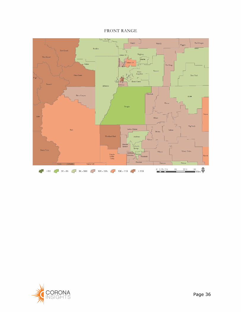
Page 36
FRONT RANGE

Page 37
EXHIBIT D: MAPS OF THE HEALTHCARE INDEX, 2019
STATEWIDE

Page 38
APPENDIX B: CHANGES FROM THE 2017 STUDY
AND IMPLICATIONS
The 2019 Cost of Living Study includes several substantive changes from previous studies. In planning for
the 2019 study, Corona took into account input from the Legislative Council as well as our own review of past
years’ research. We identified several areas for improvement this year, and then worked to balance the added
scope with time and budget restraints. Below we highlight key decisions made as part of this planning process
and their impact on the results of the study.
Shopping patterns. Since 2013, the cost of living analysis was supported by a shopping patterns
database constructed from survey data collected by Corona Insights in 2007, 2009 and 2011.
Although this database included responses from 7,864 households, it had not been updated in
nearly a decade. During that time, some areas of Colorado have seen substantial growth or decline
in retail market areas, such as along the I-25 corridor or in rural communities. Additionally,
national studies have demonstrated a steady increase of online shopping volume. For these
reasons, we suggested conducting a large-scale mail back survey to reevaluate the shopping
patterns within each district. This investment would ensure the integrity of the final results and
index.
Updating the shopping patterns using a survey approach required a substantial investment,
including survey development, mapping, sampling, data entry and analysis, in addition to costs for
printing, mailing, and postage. To fit this investment within the budget available for this year’s
study, Corona researched data patterns from prior studies, searching for opportunities to increase
efficiency with minimal loss of data accuracy or reliability. An acceptable approach that we
adopted this year was reducing the number of market basket items and collecting prices online or
over the phone, rather than in person. We describe these choices and implications below.
Reducing the number of market basket items. In planning for the 2019 study we undertook
a significant review of the market basket items. We evaluated how much of overall expenditures
were represented by each item, how widely available each item was in recent years, and whether
the items captured typical levels of variation between districts for items in their category. For
example, in 2017, there were 16 food items included in the market basket and food accounted for
14 percent of spending for the benchmark household; apparel had 6 market basket items and
accounted for 3 percent of household spending; personal care had 5 items and accounted for 1%
of household spending. Because there is a large cost in data collection for each additional item in
the market basket, items representing less than one half of one percent of spending received
additional scrutiny. For those items, we examined how widely available they were, with a
preference for items where a substantially similar item was available in a large number of districts.
Apparel items were especially low on this measure with most items available in only 30 percent of
districts, and additional concerns about item consistency across districts. Food and personal care
items were more widely available, and there were not large differences between items in
availability. Finally, we examined the price variability of items between districts. Items with low
variability between districts do not have much impact on the index but incur the same cost in data
collection. Of particular note were alcohol and tobacco prices, which had very low variability
between districts, and each represented less than one percent of spending. These items were good
candidates for including in the items held constant in the market basket. For items like food and
personal care, we looked at the range of price variation across items and prioritized items that

Page 39
were in the middle of the range for their category. To summarize, we included items that best fit
four criteria:
1. A commonly purchased item that was representative of the category of spending (i.e., had
face validity)
2. The item represented a significant proportion of spending (i.e., greater than 0.5%), and
was from the largest subcategory of spending within the category (e.g., fresh fruit was the
largest subcategory of spending within the fruit and vegetables subcategory of food at
home).
3. Widely available across districts in substantially similar form (e.g., bananas for sale in
Cortez are very similar to bananas for sale in Sterling)
4. Where reducing the number of items representing a subcategory, retain the item with an
average level of variability across districts. For example, if the category has been
represented by three items in the past, and one of those items does not vary at all between
districts, and one varies a lot between districts, choose the item in the middle to best
represent the range of items in the category. Our analysis found that items within most
categories showed similar levels of variation between districts. There were however
differences between categories, most notably the low variation in alcohol and tobacco
prices, resulting in our recommendation to treat those items as constant spending across
districts in 2019.
Finally, to explore the impact of a reduced market basket on the index, we ran simulations with
prior year data to calculate the index as if we had collected the reduced market basket rather than
the full basket. The implications for the index were minimal, with a very high correlation between
outcomes – utilizing the reduced market basket predicted 98 percent of the variance of the
previous study.
Other changes to the market basket. In reviewing the market basket items, the item that was
least satisfying in terms of our criteria was the refrigerator in the household furnishings and
equipment category. It has consistently been a challenge to find an item for this category that is
widely available and substantially similar everywhere. The category specifications for this item
from CES include both large and small appliances, as well as decorative items, tools, and smoke
alarms. We visited a variety of businesses to investigate item availability at hardware and general
stores and similarity of items offered across stores. We considered coffee makers, toasters, screw
drivers, and smoke detectors among other products, and our assessment was that smoke detectors
were the most widely available in a consistent product specification, so we recommended
including a smoke detector in the market basket for 2019. Our store visits also revealed that it was
going to be harder to price a substantially similar coffee item across stores as there are now many
more varieties of coffee sold even within brands. We considered and test shopped a variety of
alternative items within the “other food at home” category and determined that a 2-liter bottle of
Coca-Cola was the most consistently available product for pricing, so we recommended including
this item in the market basket for 2019.
Field data collection. In past years, most retail and dining prices were gathered by in-person
visits to stores. While in-person data collection is often ideal, it is cost and time intensive. To free
up budget to be applied to the above changes, Corona collected pricing for a reduced set of retail
and dining market basket items (e.g., groceries, pizza, etc.) via telephone. Corona first piloted the

Page 40
concept by test calling a variety of businesses to ensure we could secure accurate prices over the
phone. We then visited many of those businesses to establish that we were in fact receiving the
correct price. Training guides and scripts were then developed for data collectors.
Some items were able to be collected online. Here again, Corona conducted a test to verify that
prices gathered online at these stores would match the price in store. Data collectors were then
trained on the specific way to gather these prices online to ensure the right item and store were
selected. Stores where prices were collected online included King Soopers/City Market, Target,
and Walmart. Other stores, such as Safeway, were tested, but did not prove to be reliable. Not all
locations were able to be collected online. In those situations, phone calls were still made.
Adding housing rent to the market basket. It is our understanding that dwelling rent was not
included in any of the previous cost of living studies. Prior studies assumed the benchmark
household owned the home in which they lived. However, home ownership rates vary
substantially across districts, from 92 percent in Elizabeth District to 48 percent in Harrison
District, according to the U.S. Census Bureau’s American Community Survey. Further, rental
costs do not trend exactly with ownership costs. In this study, Corona incorporated dwelling rent
to produce a more robust analysis of the cost of living than relying on home ownership costs
alone. Including rent notably impacted the influence of extreme housing values (such as in Aspen
District) on the overall index and within the housing sub-index.
Accounting for geographic overlap. There are 64 counties in Colorado, 455 census designated
places (i.e., cities, towns, and housing communities), 526 ZIP codes, over 246,000 census blocks,
and 178 school districts. While a handful of school districts exactly match some of these
jurisdictions (e.g., Douglas County and Douglas County School District match exactly), most
school districts do not exactly match other geographic boundaries. Some data, such as day care
costs, are available by county, while other data, such as water, are mostly available by census
designated place. It is our understanding that the 2017 and 2015 studies matched each school
district to only one county, city, or ZIP code, and any value associated with that geography was
appropriated to the school district completely. In this study, we improved this process by first
determining the proportion of households within various geographic combinations, and we used
those proportions to allocate values from counties and cities to school districts. This approach is
more robust than assuming that school districts do not overlap other geographic boundaries.
Applying sales tax. Similar to the discussion above about accounting for geographic overlap,
sales taxes vary notably by geography. For example, St. Vrain School District includes taxing
jurisdictions of Longmont, Niwot, unincorporated Boulder County, Fredrick, Firestone,
unincorporated Weld County, and parts of the district are within the Regional Transportation
District. It is our understanding that the 2017 and 2015 studies assigned sales taxes without
accounting for the proportion of businesses or households within each unique taxing jurisdiction.
This study, however, does assign every household and business to its unique taxing jurisdiction,
so the results represent a more realistic assessment of the cost of living.
Standardizing natural gas rates. It is our understanding that previous cost of living studies
measured natural gas costs as natural gas revenue divided by the number of natural gas customers
for each utility. While that approach does reflect the amount of money spent on natural gas, it
does not appropriately reflect the relative cost per unit of natural gas. Home sizes vary across
districts, and larger homes typically use more natural gas for heating. Previous calculations that
divided revenue by number of customers were more reflective of the amount of natural gas used

Page 41
than the cost for natural gas. In this study, we improved this process by calculating the cost per
unit of natural gas for each utility, then calculated a standardized natural gas bill based on the
benchmark household using 750 Therms of natural gas per year.
Applying propane rates to rural households. Unlike electric utilities, natural gas providers generally do not publicly share their service area boundaries, because the information is proprietary. And unlike access to electric service, which is widespread, access to natural gas service is much more limited to urban areas and corridors between urban areas. Thus, households in rural parts of districts are unlikely to have natural gas access, even if urban parts of that same district do have natural gas access. Previous studies assumed that if natural gas was provided anywhere in the district, then all households in the district had access. In this study, however, we assume that households outside of census designated places do not have natural gas access and therefore rely on propane, which is more likely to accurately reflect the cost of living in rural districts where natural gas is accessible by only a small proportion of households.

Page 42
APPENDIX C: STATISTICAL MEASURES &
TECHNIQUES USED IN THIS REPORT
This appendix is reproduced from previous cost of living reports to ensure that this information on the
development of confidence intervals is available to readers each year. Confidence intervals reflect the
uncertainty arising from the fact that every store in the state is not visited. The general concept employed in
this methodology is the propagation of uncertainty. Uncertainty propagation examines how the uncertainty in
a calculated result depends on the uncertainty in the measured values that are entered into the formula. The
generalized equation for error propagation for a function f(x, y, z …) where variables x, y and z are uncorrelated
is:
...2
2
2
2
2
2
2 +
+
+
= zyxf
z
f
y
f
x
f [1]
where 2
i is the variance of variable i. For this project, we are interested in determining the variances (the 95%
confidence interval of f is approximately f96.1 ) of the cost of living index ),,,( wpSfCOL D= where
D are the mean prices of consumer products in the district, S are the shopping patterns, p are the decimal
population fractions in each district, and w are weights that determine the contributions of individual consumer
products to the overall cost of living. All four of these variable types are estimated from surveys of one type or
another, and hence have error associated with them. However, only the errors in the district consumer prices
D are considered in the Bengtsson treatment.
The Bengtsson derivations for the propagation of D errors are approximate in that equation [1] is not
applied directly to the COL function. Rather, for simplicity, equation [1] is applied successively to components
of the COL function in order to build up the final expression for 2
f . This simplification is probably necessary
given the complexity of the COL function. An amplification of the derivation of the variances of interest is
provided later. The conceptual part of this appendix will address some key questions.
Does a large variance in the item cost data automatically translate to a large confidence interval? Consider that you wanted
to get a haircut in Aspen. It is likely that you could find haircuts ranging from around $20 to well over $100,
leading to a large variance in the price of haircuts in Aspen. Does this necessarily mean that the cost of living
index will have a large confidence error? No, because the confidence interval depends on the variance of the
estimate of the mean price as opposed to the variance of the sample. But districts with large price variances do
require more intensive sampling. Consider a simplified example where there are 20 places to get a haircut in
Aspen, and at half of them you can get a $20 haircut and at the other half haircuts cost $100. Let’s also assume
that by chance whenever we sample haircut prices that we sample equally between the two haircut prices. Table
1 illustrates what happens to the variance and 95% confidence interval of the estimate of the mean price as a
function of number of prices sampled.

Page 43
Variance and Confidence Interval of Mean Price Estimate as a Function of Sample Size
N Estimate of Mean
Price
Variance of
Sample
Variance of
Estimate of Mean
Price
95% Confidence
Interval of Estimate of
Mean Price
2 $60 3200 1516 $76
4 $60 2133 449 $42
8 $60 1829 144 $24
16 $60 1797 24 $10
While this example is somewhat extreme, it does illustrate that large variances in the district prices can be
overcome by more intensive sampling. However, a question arises; are the higher priced haircuts even pertinent
to the middle-income population targeted by the study, given the availability of lower priced haircuts?
Seemingly, much of this problem would go away with a combination of strict item criteria and careful outlier
detection process. If additional sampling of certain districts is indicated by large CI, more detailed outlier
removal for that shopping district may be indicated.
Does a large CI always signal a need for additional price sampling? The primary motivation of determining
confidence intervals of COL indices is to determine if additional sampling is needed. The question arises, is
additional sampling always in indicated when the CI is large? Probably not. Consider a rural area where there
may be one grocery store in which the majority of people shop, but also several small convenience stores with
somewhat higher prices. Provided the initial price sampling included the grocery store, additional sampling of
convenience stores will likely artificially inflate the mean price. The uncertainty in the size of the shopping
universe also complicates this situation (see first paragraph of the appendix). As the number of stores sampled
(n) approaches the number of stores in the universe of stores (U), the uncertainty in the mean price estimate
approaches zero. So, in a small district with large price variances, the strategy for reducing the CI would be to
sample every store. However, in some cases the number of stores sampled to date exceeded the supposed value
of U. This uncertainty of U makes it difficult to be certain that every store has been sampled. The need to
increase sampling of high CI districts needs to be evaluated on a case by case basis. Most of the challenges
described so far could be eliminated with store-specific shopping patterns for the target income group.
However, reliable collection of such data is probably impossible.
What are the limitations of the method used to calculate the confidence intervals of the COL indices? One of the major
limitations of the method of calculating CI is that only uncertainty in mean district prices is taken into account.
There is also likely to be uncertainty in the shopping patterns, which also propagates through the calculation
and would affect the uncertainty in the COL indices. There may also be smaller errors associated with the
weighting and population factors, depending on what these measures are designed to represent. Mathematically,
the derivation of an analytical expression to propagate uncertainty in the district prices, shopping patterns, and
other sources of uncertainty may be difficult. A Monte Carlo method may be more practical. However, given
the expected size of the uncertainty in the shopping patterns, the overall uncertainty in the COL indices, if
additional factors are included, may appear to be unacceptably large without prior education.
Alternatively, a separate CI interval could be calculated using uncertainty of the shopping pattern alone,
without consideration of the uncertainty in shopping patterns. The purpose of this CI would be to determine
if additional surveying of shopping patterns is needed.

Page 44
What does the confidence interval actually tell us? The confidence interval as calculated by the Bengtsson method
indicates the level of uncertainty in the COL indices as affected by uncertainty in the prices available to
consumers. It does not reflect the overall uncertainty in the mean COL estimates. It can be used as a screening
tool to identify districts that may potentially benefit from additional price sampling. However, once identified,
some additional consideration needs to be given to whether additional price sampling would actually be
beneficial or whether tools such as outlier detection may be more appropriate. In general, shopping areas that
have a large number of consumer choices and large price variances may benefit from additional sampling. If
the shopping district has relatively few choices, additional sampling could help provided 1) the new stores
sampled actually capture a significant market share and 2) the total universe of stores in the district is known
with certainty.
Statistical Appendix
To illustrate the application of equation 1 to the COL function and to aid in decoding the vector notation
in the Bengtsson methodology, we will consider a simple case in which there are two school districts and three
shopping districts in the state. For each consumer item that contributes to the COL index, we estimate the
mean price within the district D by a shopping survey of a subset n of the stores. We also calculate the
variance of the sample D from the sample data. The variance of the estimate of D is given by nD
22 = ,
which is also the square of the standard error of the sample. As n approaches the total number of stores that
have that item (U), the accuracy of our estimate of D increases. We account for this effect on 2
by
multiplying by the factor )1()( −− UnU . So, for our example we have: )',,( 321 DDD =Dμ and
)',,( 2
3
2
2
2
1 =μσ . We also have the shopping pattern matrix (note that the shopping matrix assembled
by Corona Insights is actually S’ as shown below):
=
23
13
2221
1211'
S
S
SS
SSS [2]
The actual prices paid by consumer in the district is the shopping-pattern-weighted costs DD μSμ '=S . If
we expand this for school district 1 we get:
3132121111 DDDSD SSS ++= [3]
If we now apply equation [1] to find 2
1 S(the variance of 1SD ):
2
3
2
13
2
2
2
12
2
1
2
11
2
3
2
3
12
2
2
2
12
1
2
1
12
1
SSS
D
SD
D
SD
D
SDS ++=
+
+
=
This corresponds to the vector notation:
SSS
22 ' =
where 2
and 2
S are square matrices with the elements of interest on the diagonals.

Page 45
The state-average price is given by:
323213122221211212111
32322212123132121111
)()()(
)()(
DDD
DDDDDDSS
SpSpSpSpSpSp
SSSpSSSp
+++++=
+++++=
To find the variance of the state-average price we again apply equation [1]:
2
3
2
232131
2
2
2
222121
2
1
2
212111
2
3
2
3
2
2
2
2
2
1
2
1
2
)()()(
SpSpSpSpSpSp
D
SS
D
SS
D
SSSS
+++++=
+
+
=
This corresponds to the vector notation:
SpSpSS
22 '' = ← imagine this in bold
The COL is a weighted function of the ratios SSSDDr = . Now for district 1 we calculate the variance
2
1r of the ratio SSSDDr 11 = by application of equation [1] again, remembering that the variances of 1SD
and SS are 2
1 S and 2
SS , respectively:
( )22
1
2
12
2
4
2
12
12
2
2
2
1
2
1
2
1
11SSDS
SS
SS
SS
SDS
SS
SS
SS
DS
SD
Dr
r
rr
+=+=
+
=
where we assume 1Dr can be approximated by 1. Finally, the cost of living index over i items is given by:
= DiirwCOL
and its variance is given by:
222
riiCOL w =

Page 46
APPENDIX D: RAW PRICING DATA FOR
SELECTED PURCHASE CATEGORIES
This appendix provides the raw pricing data that underpins the analysis. Readers receiving this report
electronically will need to review an accompanying spreadsheet file, due to the volume of data.

Page 47
APPENDIX E: SHOPPING PATTERNS SURVEY
INSTRUMENT
The survey instruments used for the shopping patterns survey are provided on the following pages. This
includes the cover letter, the survey used for non-Front Range areas, and one sample of a Front Range survey
plus the map provided where respondents answered according to the “zone” they made their purchase within.
Envelopes and postcard reminders are not shown.
The online versions of these surveys contained the same questions, but were formatted to take into account
online, including mobile phone, usability.

Cover Letter
Used for all surveys

Bright thinking. Brilliant guidance.
1580 Lincoln Street, Suite 510 Denver, CO 80203 P303.894.8246 F303.894.9651 CoronaInsights.com
October 18, 2019 Greetings, Corona Insights, a local Colorado research firm, is conducting a study to understand shopping locations for residents throughout Colorado. Corona Insights has conducted this study multiple times since 2007 and are currently updating figures for 2019, and we could use your help. This information is used to benefit local communities throughout the state. We’re conducting the enclosed short survey to figure out where people shop and ask that you take approximately five minutes to fill it out, then return it to us in the enclosed postage-paid envelope. Please take this survey at your earliest convenience. By completing this survey, you will have an opportunity to win one of five $50 Visa gift cards. This is our simple way of thanking you for your time and input. We hope you enjoy completing the questionnaire and look forward to receiving your response.
Sincerely,
Matt Bruce Director, Corona Insights
If you have trouble with the survey, contact Matt Bruce of Corona Insights at [email protected] or 303-894-8246. For the official rules for the Cost of Living $50 Gift Card Sweepstakes, please visit www.CoronaInsights.com/ShoppingRules.

Survey: No Zones
Used for non-Front Range Regions

Page 1
1. On this page, please tell us where you or a member of your household usually purchase each item in the list below. Write the name of the city or town where you usually buy that item. If you usually buy the item online, check the box in the online column. Lastly, if you or a member of your household never purchase the item, check the box in the never purchase column.
Tell us the name of that City or Town Check box Check box
Example 1: you usually buy this item in Greeley City: ______________
Example 2: you usually buy this item online City: ______________
City: ______________
City: ______________
City: ______________
City: ______________
City: ______________
(If you ordered online, list the city or town where the store is located)
City: ______________
(not a bar or restaurant) City: ______________
City: ______________
City: ______________
City: ______________
City: ______________
(If you bought your tickets online, list the zone or town where you saw the movie.)
City: ______________
(men’s or women’s) City: ______________
Greeley
X

Page 2
We’ll now ask about less frequent purchases.
2. Have you, or someone in your household, purchased a small appliance (such as a blender, coffee maker, etc.) in the past 2 years? Please check one.
Yes, I bought this item while living in my current region(Please answer 2a)
Yes, but I bought this item while living in different region(Please answer 2b)
No, I have not purchased in the past 2 years(Please answer 2b)
2a. In what city or town did you make your most recent small appliance (such as a blender, coffee maker, etc.) purchase?
2b. If you were going to buy a small appliance, in what city or town do you think you would you do so?
(Please print clearly)
__________
Check box
(Please print clearly)
__________
Check box
3. Have you, or someone in your household, purchased a television in the past 2 years? Please check one.
Yes, I bought this item while living in my current region(Please answer 3a)
Yes, but I bought this item while living in different region(Please answer 3b)
No, I have not purchasedin the past 2 years(Please answer 3b)
3a. In what city or town did you make your most recent television purchase?
3b. If you were going to buy a television, in what city or town do you think you would you do so?
(Please print clearly)
__________
Check box
(Please print clearly)
__________
Check box

Page 3
Now we just have a few questions about housing prices and locations.
4. Which of the following best describes your home? Please check one.
Single family home, not attached to other units
Part of a 2-, 3-, or 4-unit structure (such as a duplex, triplex, or fourplex)
In a building with 5 to 19 housing units
In a building with 20 or more units
A mobile home
Some other type of housing unit Please tell us:
5. How many bedrooms are in your home? Please write a number. If it’s a studio or buffet unit, write “0”.
6. Do you rent or own your home? Please check one.
Own
Rent
Other Please tell us:
Don’t Know
7. How much do you agree or disagree with the following statement: I usually try new products before other people do.
Strongly Disagree
Disagree
Agree
Strongly Agree

Page 4
Our last questions are about you and your location, so we can map and analyze the data.
8. Are you…?
Male
Female
Prefer to self-describe Please tell us:
9. In what year were you born? Please enter a 4-digit year.
10. Please tell us more about your location.
City (or nearest city): County: Zip:
11. Which category best describes the occupation(s) of the adults (age 18 and older) in your household? Please select the occupations for all members of your household.
Employed by a for-profit company or business or individual
Employed by a not-for-profit, tax-exempt, or charitable organization
Government employee (Local, State, or Federal)
Military
Teacher (K-12)
Self-employed
Student
Retiree
Homemaker
Other
Thank you. We appreciate your time.
If you would like to enter the sweepstakes for a chance to win one of five $50 Visa Gift Cards, please include your contact information below. Your responses will remain confidential. For the official rules for the Sweepstakes, please visit: CoronaInsights.com/ShoppingRules or contact (303) 894-8246 or [email protected]. You do not have to complete a survey to be entered into the Sweepstakes. See the rules for alternate means of entry.
Name: __________________
Telephone: __________________
Email: __________________
Version: #.####

Survey: With Zones
Denver Region Example
Specific survey used in Denver. Similar survey used in other Front Range regions including: Colorado Springs, Northern Colorado, and the region between Metro Denver
and Northern Colorado.

Page 1
1. On this page, please tell us where you or a member of your household usually purchase each item in the list below. If you usually buy the item in the Denver Metro area, please use the enclosed maps to find the zone where you usually purchase the item, then write the zone letter below. However, if you usually buy the item outside the Denver Metro area, write the name of the city or town where you usually buy that item. If you usually buy the item online, check the box in the online column. Lastly, if you or a member of your household never purchase the item, check the box in the never purchase column.
Tell us the zone from enclosed map
Tell us the name of that City or Town Check box Check box
Example 1: you usually buy this item in Arvada Zone: ____ City:
___________
Example 2: you usually buy this item in Greeley Zone: ____ City:
___________
Example 3: you usually buy this item online Zone: ____ City:
___________
Zone: ____ City: ___________
Zone: ____ City: ___________
Zone: ____ City: ___________
Zone: ____ City: ___________
Zone: ____ City: ___________
(If you ordered online, list the city or town where the store is located)
Zone: ____ City: ___________
(not a bar or restaurant)
Zone: ____ City: ___________
Zone: ____ City: ___________
Zone: ____ City: ___________
Zone: ____ City: ___________
Zone: ____ City: ___________
(If you bought your tickets online, list the zone or town where you saw the movie.)
Zone: ____ City: ___________
(men’s or women’s) Zone: ____ City: ___________
Greeley
Q
X

Page 2
We’ll now ask about less frequent purchases. Again, if you or someone in your household bought the item in the Denver Metro area, please use the enclosed map to indicate in which zone you purchased the item.
2. Have you, or someone in your household, purchased a small appliance (such as a blender, coffee maker, etc.) in the past 2 years? Please check one.
Yes, I bought this item while living in my current region(Please answer 2a)
Yes, but I bought this item while living in different region(Please answer 2b)
No, I have not purchased in the past 2 years(Please answer 2b)
2a. In what city or town did you make your most recent small appliance (such as a blender, coffee maker, etc.) purchase?
2b. If you were going to buy a small appliance, in what city or town do you think you would you do so?
Tell us the zone from enclosed
map
Zone:
____
Tell us the name of that City or
Town
__________
Check box
Tell us the zone from enclosed
map
Zone:
____
Tell us the name of that City or
Town
__________
Check box
3. Have you, or someone in your household, purchased a television in the past 2 years? Please check one.
Yes, I bought this item while living in my current region(Please answer 3a)
Yes, but I bought this item while living in different region(Please answer 3b)
No, I have not purchasedin the past 2 years(Please answer 3b)
3a. In what city or town did you make your most recent television purchase?
3b. If you were going to buy a television, in what city or town do you think you would you do so?
Tell us the zone from enclosed
map
Zone:
____
Tell us the name of that City or
Town
__________
Check box
Tell us the zone from enclosed
map
Zone:
____
Tell us the name of that City or
Town
__________
Check box

Page 3
Now we just have a few questions about housing prices and locations.
4. Which of the following best describes your home? Please check one.
Single family home, not attached to other units
Part of a 2-, 3-, or 4-unit structure (such as a duplex, triplex, or fourplex)
In a building with 5 to 19 housing units
In a building with 20 or more units
A mobile home
Some other type of housing unit Please tell us:
5. How many bedrooms are in your home? Please write a number. If it’s a studio or buffet unit, write “0”.
6. Do you rent or own your home? Please check one.
Own
Rent
Other Please tell us:
Don’t Know
7. How much do you agree or disagree with the following statement: I usually try new products before other people do.
Strongly Disagree
Disagree
Agree
Strongly Agree

Page 4
Our last questions are about you and your location, so we can map and analyze the data.
8. Are you…?
Male
Female
Prefer to self-describe Please tell us:
9. In what year were you born? Please enter a 4-digit year.
10. Please tell us more about your location.
City (or nearest city): County: Zip:
11. Which category best describes the occupation(s) of the adults (age 18 and older) in your household? Please select the occupations for all members of your household.
Employed by a for-profit company or business or individual
Employed by a not-for-profit, tax-exempt, or charitable organization
Government employee (Local, State, or Federal)
Military
Teacher (K-12)
Self-employed
Student
Retiree
Homemaker
Other
Thank you. We appreciate your time.
If you would like to enter the sweepstakes for a chance to win one of five $50 Visa Gift Cards, please include your contact information below. Your responses will remain confidential. For the official rules for the Sweepstakes, please visit: CoronaInsights.com/ShoppingRules or contact (303) 894-8246 or [email protected]. You do not have to complete a survey to be entered into the Sweepstakes. See the rules for alternate means of entry.
Name: __________________
Telephone: __________________
Email: __________________
Version: #.####

Map
Denver Region Example
Specific map used in Denver. Similar maps were produced for each area that received a survey with zones.


Page 48
APPENDIX F: SHOPPING PATTERNS MATRICES
This appendix provides the geographic shopping patterns matrix used in this analysis. The matrix is based
on a survey of Colorado residents conducted in the fall of 2019. Data from this survey, in conjunction with
mathematical modeling methods, were used to construct a geographic shopping matrix describing where the
residents of each school district typically purchase particular products (i.e., what proportion of purchases are
made in the home district, in each neighboring district, online, etc.). Readers of this report will need to review
an accompanying spreadsheet file due to the volume of data.