2017 OLC Baker County - Oregon Department of Geology and … · 2018-08-30 · OLC Baker County...
19
www.quantumspatial.com January 19, 2018 2017 OLC Baker County
Transcript of 2017 OLC Baker County - Oregon Department of Geology and … · 2018-08-30 · OLC Baker County...
www.quantumspatial.com
January 19, 20182017 OLC Baker County
ii
Prepared by: Quantum Spatial
421 SW 6th AvenueSuite 800Portland, OR 97204phone: (503) 505-5100fax: (503) 546-6801
517 SW 2nd StreetSuite 400Corvallis, OR 97333phone: (541) 752-1204fax: (541) 752-3770
Data collected for: Oregon Department of Geology and Mineral Industries
800 NE Oregon StreetSuite 965Portland, OR 97232
1
Overview
Contents
2 - Project Overview 4 - Deliverable Products 6 - Aerial Acquisition
6 - LiDAR Survey
7 - Ground Survey7 - Instrumentation7 - Monumentation7 - Methodology
10 - Processing10 - LiDAR Processing11 - LAS Classification Scheme11 - Hydro-Flattened Breaklines11 - Hydro-Flattened Raster DEM Creation
12 - LiDAR Accuracy Assessments12 - Relative Vertical Accuracy13 - Absolute Vertical Accuracy
14 - Density14 - Pulse Density15 - Ground Density
17 - Appendix A : Certifications
2
Overview
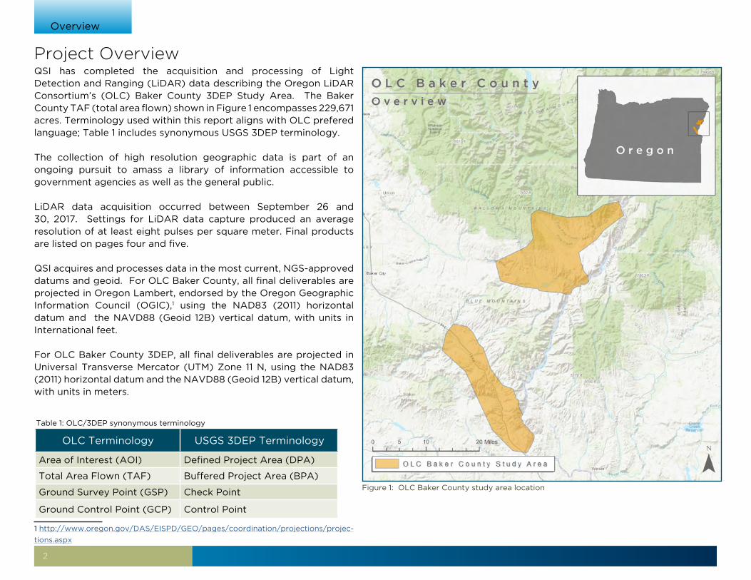
QSI has completed the acquisition and processing of Light Detection and Ranging (LiDAR) data describing the Oregon LiDAR Consortium’s (OLC) Baker County 3DEP Study Area. The Baker County TAF (total area flown) shown in Figure 1 encompasses 229,671 acres. Terminology used within this report aligns with OLC prefered language; Table 1 includes synonymous USGS 3DEP terminology.
The collection of high resolution geographic data is part of an ongoing pursuit to amass a library of information accessible to government agencies as well as the general public.
LiDAR data acquisition occurred between September 26 and 30, 2017. Settings for LiDAR data capture produced an average resolution of at least eight pulses per square meter. Final products are listed on pages four and five.
QSI acquires and processes data in the most current, NGS-approved datums and geoid. For OLC Baker County, all final deliverables are projected in Oregon Lambert, endorsed by the Oregon Geographic Information Council (OGIC),1 using the NAD83 (2011) horizontal datum and the NAVD88 (Geoid 12B) vertical datum, with units in International feet.
For OLC Baker County 3DEP, all final deliverables are projected in Universal Transverse Mercator (UTM) Zone 11 N, using the NAD83 (2011) horizontal datum and the NAVD88 (Geoid 12B) vertical datum, with units in meters.
1 http://www.oregon.gov/DAS/EISPD/GEO/pages/coordination/projections/projec-
tions.aspx
Project Overview
Figure 1: OLC Baker County study area location
OLC Terminology USGS 3DEP Terminology
Area of Interest (AOI) Defined Project Area (DPA)
Total Area Flown (TAF) Buffered Project Area (BPA)
Ground Survey Point (GSP) Check Point
Ground Control Point (GCP) Control Point
Table 1: OLC/3DEP synonymous terminology
3
Overview
Project Overview
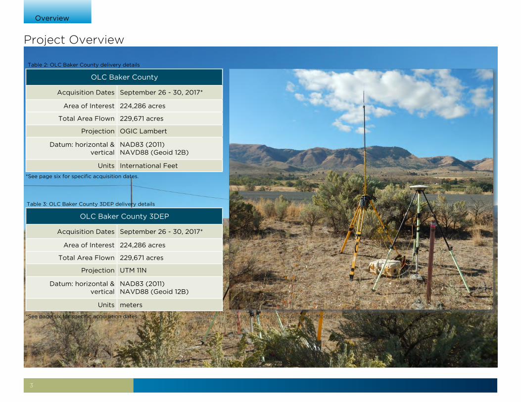
Table 2: OLC Baker County delivery details
*See page six for specific acquisition dates.
OLC Baker County 3DEP
Acquisition Dates September 26 - 30, 2017*
Area of Interest 224,286 acres
Total Area Flown 229,671 acres
Projection UTM 11N
Datum: horizontal & vertical
NAD83 (2011)NAVD88 (Geoid 12B)
Units meters
Table 3: OLC Baker County 3DEP delivery details
*See page six for specific acquisition dates.
Figure 2: Zephyr GNSS Geodetic Model 2 antenna set up over QB0516 NGS monument
OLC Baker County
Acquisition Dates September 26 - 30, 2017*
Area of Interest 224,286 acres
Total Area Flown 229,671 acres
Projection OGIC Lambert
Datum: horizontal & vertical
NAD83 (2011)NAVD88 (Geoid 12B)
Units International Feet
4
Overview
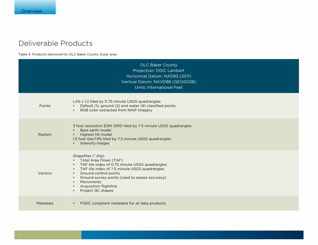
Table 4: Products delivered for OLC Baker County study area.
Deliverable Products
OLC Baker County
Projection: OGIC Lambert
Horizontal Datum: NAD83 (2011)
Vertical Datum: NAVD88 (GEOID12B)
Units: International Feet
PointsLAS v 1.2 tiled by 0.75 minute USGS quadrangles• Default (1), ground (2) and water (9) classified points• RGB color extracted from NAIP imagery
Rasters
3 foot resolution ESRI GRID tiled by 7.5 minute USGS quadrangles• Bare earth model• Highest hit model1.5 foot GeoTiffs tiled by 7.5 minute USGS quadrangles• Intensity images
Vectors
Shapefiles (*.shp)• Total Area Flown (TAF)• TAF tile index of 0.75 minute USGS quadrangles• TAF tile index of 7.5 minute USGS quadrangles• Ground control points• Ground survey points (used to assess accuracy)• Monuments• Acquisition flightline• Project QC shapes
Metadata • FGDC compliant metadata for all data products
5
Overview
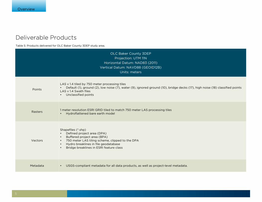
Table 5: Products delivered for OLC Baker County 3DEP study area.
Deliverable Products
OLC Baker County 3DEP
Projection: UTM 11N
Horizontal Datum: NAD83 (2011)
Vertical Datum: NAVD88 (GEOID12B)
Units: meters
Points
LAS v 1.4 tiled by 750 meter processing tiles• Default (1), ground (2), low noise (7), water (9), ignored ground (10), bridge decks (17), high noise (18) classified pointsLAS v 1.4 Swath files• Unclassified points
Rasters1 meter resolution ESRI GRID tiled to match 750 meter LAS processing tiles• Hydroflattened bare earth model
Vectors
Shapefiles (*.shp)• Defined project area (DPA)• Buffered project area (BPA)• 750 meter LAS tiling scheme, clipped to the DPA• Hydro breaklines in file geodatabase • Bridge breaklines in ESRI feature class
Metadata • USGS-compliant metadata for all data products, as well as project-level metadata.
6
Aerial Acquisition
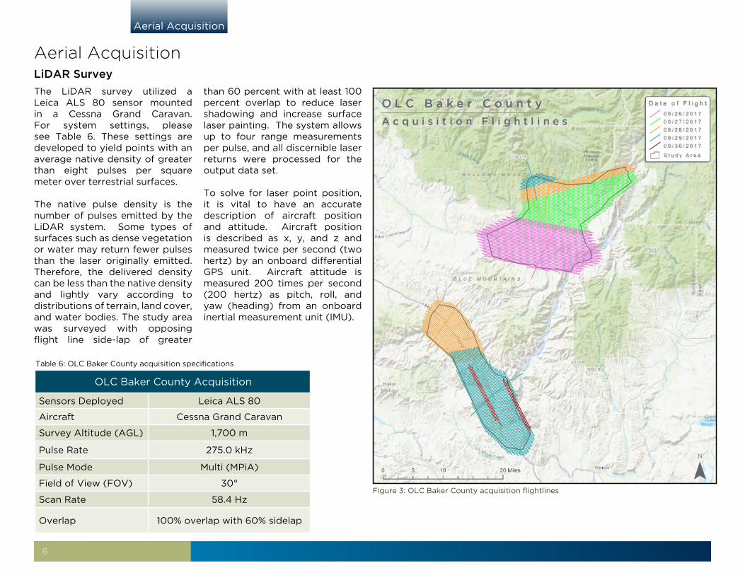
The LiDAR survey utilized a Leica ALS 80 sensor mounted in a Cessna Grand Caravan. For system settings, please see Table 6. These settings are developed to yield points with an average native density of greater than eight pulses per square meter over terrestrial surfaces.
The native pulse density is the number of pulses emitted by the LiDAR system. Some types of surfaces such as dense vegetation or water may return fewer pulses than the laser originally emitted. Therefore, the delivered density can be less than the native density and lightly vary according to distributions of terrain, land cover, and water bodies. The study area was surveyed with opposing flight line side-lap of greater
than 60 percent with at least 100 percent overlap to reduce laser shadowing and increase surface laser painting. The system allows up to four range measurements per pulse, and all discernible laser returns were processed for the output data set.
To solve for laser point position, it is vital to have an accurate description of aircraft position and attitude. Aircraft position is described as x, y, and z and measured twice per second (two hertz) by an onboard differential GPS unit. Aircraft attitude is measured 200 times per second (200 hertz) as pitch, roll, and yaw (heading) from an onboard inertial measurement unit (IMU).
Aerial AcquisitionLiDAR Survey
OLC Baker County Acquisition
Sensors Deployed Leica ALS 80
Aircraft Cessna Grand Caravan
Survey Altitude (AGL) 1,700 m
Pulse Rate 275.0 kHz
Pulse Mode Multi (MPiA)
Field of View (FOV) 30°
Scan Rate 58.4 Hz
Overlap 100% overlap with 60% sidelap
Table 6: OLC Baker County acquisition specifications
Figure 3: OLC Baker County acquisition flightlines
7
Ground Survey
Ground control surveys were conducted to support the airborne acquisition. Ground survey data, including monumentation, ground control points (GCPs), and ground survey points (GSPs), are used to geospatially correct the aircraft positional coordinate data and to perform quality assurance checks on final LiDAR data.
Instrumentation
All Global Navigation Satellite System (GNSS) static surveys utilized Trimble R7 GNSS receivers with Zephyr Geodetic Model 2 RoHS antennas. Rover surveys for GCP and GSP collection were conducted with Trimble R10 GNSS receivers. See Table 8 for specifications of QSI equipment used.
Monumentation
Ground Survey
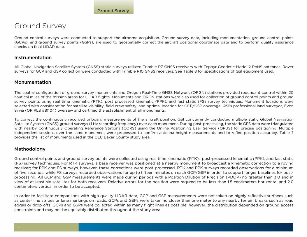
The spatial configuration of ground survey monuments and Oregon Real-Time GNSS Network (ORGN) stations provided redundant control within 20 nautical miles of the mission areas for LiDAR flights. Monuments and ORGN stations were also used for collection of ground control points and ground survey points using real time kinematic (RTK), post processed kinematic (PPK), and fast static (FS) survey techniques. Monument locations were selected with consideration for satellite visibility, field crew safety, and optimal location for GCP/GSP coverage. QSI’s professional land surveyor, Evon Silvia (OR PLS #81104) oversaw and certified the establishment of all monuments.
To correct the continuously recorded onboard measurements of the aircraft position, QSI concurrently conducted multiple static Global Navigation Satellite System (GNSS) ground surveys (1 Hz recording frequency) over each monument. During post-processing, the static GPS data were triangulated with nearby Continuously Operating Reference Stations (CORS) using the Online Positioning User Service (OPUS) for precise positioning. Multiple independent sessions over the same monument were processed to confirm antenna height measurements and to refine position accuracy. Table 7 provides the list of monuments used in the OLC Baker County study area.
Methodology
Ground control points and ground survey points were collected using real time kinematic (RTK), post-processed kinematic (PPK), and fast static (FS) survey techniques. For RTK surveys, a base receiver was positioned at a nearby monument to broadcast a kinematic correction to a roving receiver; for PPK and FS surveys, however, these corrections were post-processed. RTK and PPK surveys recorded observations for a minimum of five seconds, while FS surveys recorded observations for up to fifteen minutes on each GCP/GSP in order to support longer baselines for post-processing. All GCP and GSP measurements were made during periods with a Position Dilution of Precision (PDOP) no greater than 3.0 and in view of at least six satellites for both receivers. Relative errors for the position were requred to be less than 1.5 centimeters horizontal and 2.0 centimeters vertical in order to be accepted.
In order to facilitate comparisons with high quality LiDAR data, GCP and GSP measurements were not taken on highly reflective surfaces such as center line stripes or lane markings on roads. GCPs and GSPs were taken no closer than one meter to any nearby terrain breaks such as road edges or drop offs. GCPs and GSPs were collected within as many flight lines as possible; however, the distribution depended on ground access constraints and may not be equitably distributed throughout the study area.

8
Ground Survey
Figure 4: OLC Baker County study area ground survey map
Figure 5: OLC Baker County QB0516 monument
Figure 6: OLC Baker County QB0516 monument
9
Processing
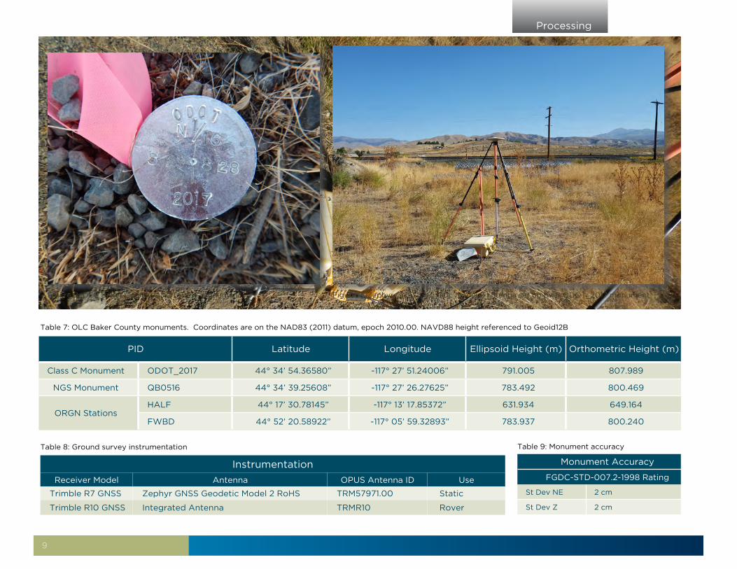
Table 7: OLC Baker County monuments. Coordinates are on the NAD83 (2011) datum, epoch 2010.00. NAVD88 height referenced to Geoid12B
Figure 7: Zephyr GNSS Geodetic Model 2 antenna set up over ODOT_2017 monument
PID Latitude Longitude Ellipsoid Height (m) Orthometric Height (m)
Class C Monument ODOT_2017 44° 34’ 54.36580” -117° 27’ 51.24006” 791.005 807.989
NGS Monument QB0516 44° 34’ 39.25608” -117° 27’ 26.27625” 783.492 800.469
ORGN StationsHALF 44° 17’ 30.78145” -117° 13’ 17.85372” 631.934 649.164
FWBD 44° 52’ 20.58922” -117° 05’ 59.32893” 783.937 800.240
Table 8: Ground survey instrumentation
Instrumentation
Receiver Model Antenna OPUS Antenna ID Use
Trimble R7 GNSS Zephyr GNSS Geodetic Model 2 RoHS TRM57971.00 Static
Trimble R10 GNSS Integrated Antenna TRMR10 Rover
Monument Accuracy
FGDC-STD-007.2-1998 Rating
St Dev NE 2 cm
St Dev Z 2 cm
Table 9: Monument accuracy
Figure 8: OLC Baker County ODOT_2017 monument
10
Processing
This section describes the processing methodologies for all data acquired by QSI for the 2017 OLC Baker County LiDAR project.
LiDAR Processing
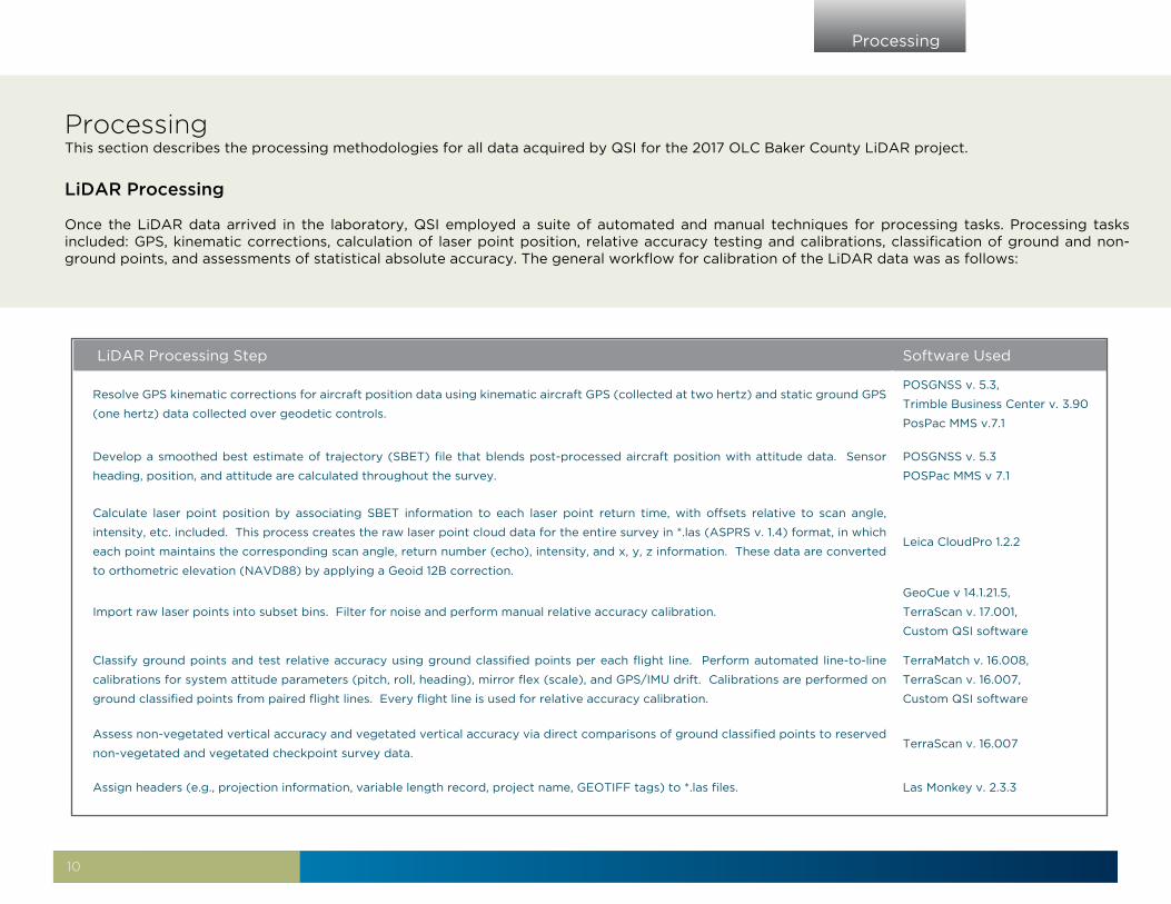
Once the LiDAR data arrived in the laboratory, QSI employed a suite of automated and manual techniques for processing tasks. Processing tasks included: GPS, kinematic corrections, calculation of laser point position, relative accuracy testing and calibrations, classification of ground and non-ground points, and assessments of statistical absolute accuracy. The general workflow for calibration of the LiDAR data was as follows:
Processing
LiDAR Processing Step Software Used
Resolve GPS kinematic corrections for aircraft position data using kinematic aircraft GPS (collected at two hertz) and static ground GPS
(one hertz) data collected over geodetic controls.
POSGNSS v. 5.3,
Trimble Business Center v. 3.90
PosPac MMS v.7.1
Develop a smoothed best estimate of trajectory (SBET) file that blends post-processed aircraft position with attitude data. Sensor
heading, position, and attitude are calculated throughout the survey.
POSGNSS v. 5.3
POSPac MMS v 7.1
Calculate laser point position by associating SBET information to each laser point return time, with offsets relative to scan angle,
intensity, etc. included. This process creates the raw laser point cloud data for the entire survey in *.las (ASPRS v. 1.4) format, in which
each point maintains the corresponding scan angle, return number (echo), intensity, and x, y, z information. These data are converted
to orthometric elevation (NAVD88) by applying a Geoid 12B correction.
Leica CloudPro 1.2.2
Import raw laser points into subset bins. Filter for noise and perform manual relative accuracy calibration.
GeoCue v 14.1.21.5,
TerraScan v. 17.001,
Custom QSI software
Classify ground points and test relative accuracy using ground classified points per each flight line. Perform automated line-to-line
calibrations for system attitude parameters (pitch, roll, heading), mirror flex (scale), and GPS/IMU drift. Calibrations are performed on
ground classified points from paired flight lines. Every flight line is used for relative accuracy calibration.
TerraMatch v. 16.008,
TerraScan v. 16.007,
Custom QSI software
Assess non-vegetated vertical accuracy and vegetated vertical accuracy via direct comparisons of ground classified points to reserved
non-vegetated and vegetated checkpoint survey data.TerraScan v. 16.007
Assign headers (e.g., projection information, variable length record, project name, GEOTIFF tags) to *.las files. Las Monkey v. 2.3.3

11
Processing
LAS Classification Scheme
The classification classes are determined by the USGS Lidar Base Specification, version 1.2 specifications and are an industry standard for the classification of LIDAR point clouds. The classes used in the dataset are as follows and have the following descriptions:
• Class 1 – Processed, but unclassified. This class covers features such as vegetation, cars, utility poles, or any other point that does not fit into another deliverable class.
• Class 2 – Bare earth ground. Points used to create bare earth surfaces.• Class 7 – Low noise. Erroneous points not meant for use below the identified ground surface.• Class 9 – Water. Point returned off water surfaces.• Class 10 – Ignored ground. Points found to be close to breakline features. Points are moved to this class from the Class 2 dataset. This class
is ignored during the DEM creation process in order to provide smooth transition between the ground surface and hydro flattened surface.• Class 17 – Bridge decks. Points falling on bridge decks.• Class 18 – High noise. Erroneous points above ground surface not attributed to real features.
Hydro-Flattened Breaklines
Class 2 LiDAR was used to create a bare earth surface model. The surface model was then used to heads-up digitize 2D breaklines of inland streams and rivers with a 100 foot nominal width and inland ponds and lakes of two acres or greater surface area.
Elevation values were assigned to all inland ponds and lakes, inland pond and lake islands, inland streams and rivers and inland stream and river islands using Quantum Spatial proprietary software
All ground (ASPRS Class 2) LiDAR data inside of the collected inland breaklines were then classified to water (ASPRS Class 9) using TerraScan macro functionality. A buffer of three feet was also used around each hydro-flattened feature. These points were moved from ground (ASPRS Class 2) to ignored ground (ASPRS Class 10).
The breakline files were then translated to Esri file geodatabase format using Esri conversion tools.
Hydro-Flattened Raster DEM Creation
Hydro flattening breaklines are merged with Class 2 LAS and set to enforce elevations within closed areas identified as water while retaining near shore lidar elevations. This process is used to ensure a downstream gradient along streams and waterbodies are level.
12
Accuracy
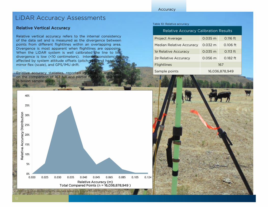
Relative Vertical Accuracy
Relative vertical accuracy refers to the internal consistency of the data set and is measured as the divergence between points from different flightlines within an overlapping area. Divergence is most apparent when flightlines are opposing. When the LiDAR system is well calibrated the line to line divergence is low (<10 centimeters). Internal consistency is affected by system attitude offsets (pitch, roll, and heading), mirror flex (scale), and GPS/IMU drift.
Relative accuracy statistics, reported in Table 10 are based on the comparison of 167 full and partial flightlines and over 16 billion sample points.
Figure 9: OLC Baker County relative accuracy based on 167 flightlines.
Relative Accuracy Calibration Results
Project Average 0.035 m 0.116 ft
Median Relative Accuracy 0.032 m 0.106 ft
1σ Relative Accuracy 0.035 m 0.113 ft
2σ Relative Accuracy 0.056 m 0.182 ft
Flightlines 167
Sample points 16,036,878,949
Table 10: Relative accuracy
0%
5%
10%
15%
20%
25%
30%
35%
40%
0.020 0.025 0.030 0.035 0.040 0.045 0.065 0.085 0.105 0.124
Re
lati
ve A
ccu
racy D
istr
ibu
tio
n
Relative Accuracy (m)Total Compared Points (n = 16,036,878,949 )
LiDAR Accuracy Assessments
13
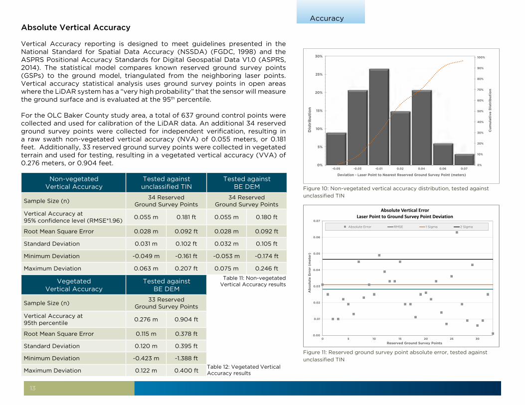
AccuracyAbsolute Vertical Accuracy
Vertical Accuracy reporting is designed to meet guidelines presented in the National Standard for Spatial Data Accuracy (NSSDA) (FGDC, 1998) and the ASPRS Positional Accuracy Standards for Digital Geospatial Data V1.0 (ASPRS, 2014). The statistical model compares known reserved ground survey points (GSPs) to the ground model, triangulated from the neighboring laser points. Vertical accuracy statistical analysis uses ground survey points in open areas where the LiDAR system has a “very high probability” that the sensor will measure the ground surface and is evaluated at the 95th percentile.
For the OLC Baker County study area, a total of 637 ground control points were collected and used for calibration of the LiDAR data. An additional 34 reserved ground survey points were collected for independent verification, resulting in a raw swath non-vegetated vertical accuracy (NVA) of 0.055 meters, or 0.181 feet. Additionally, 33 reserved ground survey points were collected in vegetated terrain and used for testing, resulting in a vegetated vertical accuracy (VVA) of 0.276 meters, or 0.904 feet.
Table 11: Non-vegetated Vertical Accuracy results
Non-vegetated Vertical Accuracy
Tested against unclassified TIN
Tested against BE DEM
Sample Size (n)34 Reserved
Ground Survey Points34 Reserved
Ground Survey Points
Vertical Accuracy at 95% confidence level (RMSE*1.96)
0.055 m 0.181 ft 0.055 m 0.180 ft
Root Mean Square Error 0.028 m 0.092 ft 0.028 m 0.092 ft
Standard Deviation 0.031 m 0.102 ft 0.032 m 0.105 ft
Minimum Deviation -0.049 m -0.161 ft -0.053 m -0.174 ft
Maximum Deviation 0.063 m 0.207 ft 0.075 m 0.246 ft
Figure 10: Non-vegetated vertical accuracy distribution, tested against
unclassified TIN
Histo Meters
Page 1
0%
10%
20%
30%
40%
50%
60%
70%
80%
90%
100%
0%
5%
10%
15%
20%
25%
30%
-0.05 -0.03 -0.01 0.02 0.04 0.06 0.07
Cu
mu
lati
ve
Dis
trib
uti
on
Dis
trib
uti
on
Deviation - Laser Point to Nearest Reserved Ground Survey Point (meters)
0.00
0.01
0.02
0.03
0.04
0.05
0.06
0.07
0 5 10 15 20 25 30
Ab
solu
te E
rro
r (m
ete
r)
Reserved Ground Survey Points
Absolute Vertical ErrorLaser Point to Ground Survey Point Deviation
Absolute Error RMSE 1 Sigma 2 Sigma
Figure 11: Reserved ground survey point absolute error, tested against
unclassified TIN
Vegetated Vertical Accuracy
Tested against BE DEM
Sample Size (n)33 Reserved
Ground Survey Points
Vertical Accuracy at 95th percentile
0.276 m 0.904 ft
Root Mean Square Error 0.115 m 0.378 ft
Standard Deviation 0.120 m 0.395 ft
Minimum Deviation -0.423 m -1.388 ft
Maximum Deviation 0.122 m 0.400 ftTable 12: Vegetated Vertical Accuracy results
14
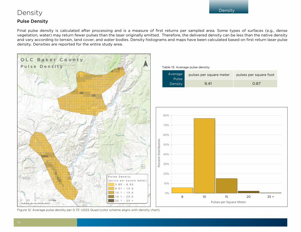
DensityDensityPulse Density
Final pulse density is calculated after processing and is a measure of first returns per sampled area. Some types of surfaces (e.g., dense vegetation, water) may return fewer pulses than the laser originally emitted. Therefore, the delivered density can be less than the native density and vary according to terrain, land cover, and water bodies. Density histograms and maps have been calculated based on first return laser pulse density. Densities are reported for the entire study area.
Figure 12: Average pulse density per 0.75’ USGS Quad (color scheme aligns with density chart).
Average
Pulse
Density
pulses per square meter pulses per square foot
9.41 0.87
Table 13: Average pulse density
Pulse Density
Page 1
0%
10%
20%
30%
40%
50%
60%
70%
80%
8 10 15 20 25 +
Perc
ent D
istrib
utio
n
Pulses per Square Meter
15
Density
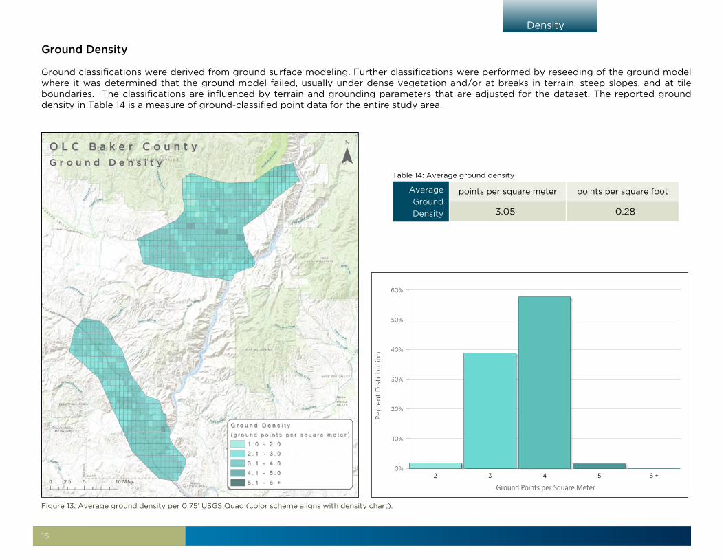
Ground Density
Ground classifications were derived from ground surface modeling. Further classifications were performed by reseeding of the ground model where it was determined that the ground model failed, usually under dense vegetation and/or at breaks in terrain, steep slopes, and at tile boundaries. The classifications are influenced by terrain and grounding parameters that are adjusted for the dataset. The reported ground density in Table 14 is a measure of ground-classified point data for the entire study area.
Figure 13: Average ground density per 0.75’ USGS Quad (color scheme aligns with density chart).
Average
Ground
Density
points per square meter points per square foot
3.05 0.28
Table 14: Average ground density
Ground Density
Page 1
0%
10%
20%
30%
40%
50%
60%
2 3 4 5 6 +
Perc
ent D
istr
ibut
ion
Ground Points per Square Meter

16
Appendix
[ Page Intentionally Blank ]
17
Appendix
Appendix A : CertificationsPLS Survey Letter
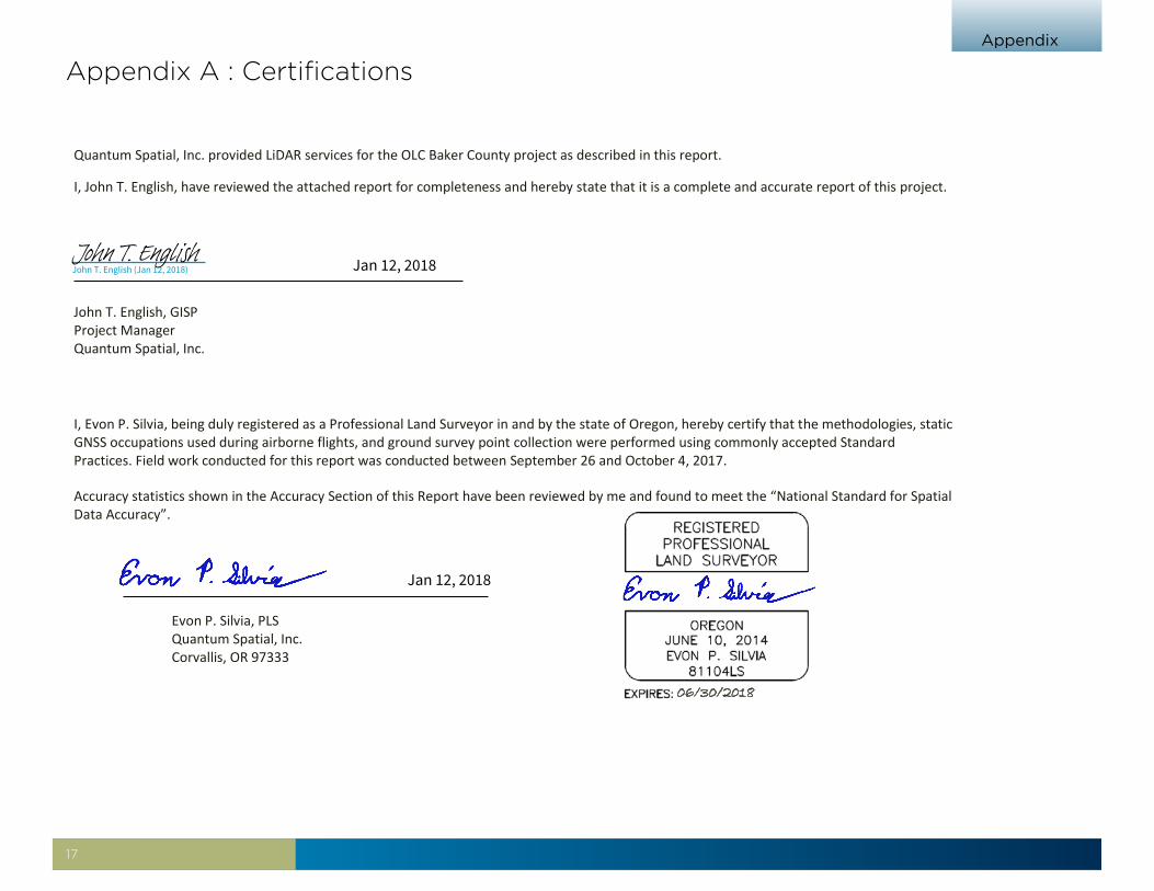
Quantum Spatial, Inc. provided LiDAR services for the OLC Baker County project as described in this report.
I, John T. English, have reviewed the attached report for completeness and hereby state that it is a complete and accurate report of this project.
John T. English, GISP Project Manager Quantum Spatial, Inc. I, Evon P. Silvia, being duly registered as a Professional Land Surveyor in and by the state of Oregon, hereby certify that the methodologies, static GNSS occupations used during airborne flights, and ground survey point collection were performed using commonly accepted Standard Practices. Field work conducted for this report was conducted between September 26 and October 4, 2017. Accuracy statistics shown in the Accuracy Section of this Report have been reviewed by me and found to meet the “National Standard for Spatial Data Accuracy”.
Evon P. Silvia, PLS Quantum Spatial, Inc. Corvallis, OR 97333
06/30/2018
Jan 12, 2018
John T. English (Jan 12, 2018)John T. English Jan 12, 2018