2017 Integrated Resource Plan - Home : PacifiCorp · Naughton 3 RH-2 Cholla 4 RH-2 Craig 1 RH-1...
91
2017 Integrated Resource Plan Public Input Meeting 7 January 26-27, 2017
Transcript of 2017 Integrated Resource Plan - Home : PacifiCorp · Naughton 3 RH-2 Cholla 4 RH-2 Craig 1 RH-1...

2017Integrated Resource Plan
Public Input Meeting 7
January 26-27, 2017

Agenda• January 26, 2017 – Day One
– Introductions
– Volume III Studies
– Lunch
– Flexible Capacity Reserve Requirements Study
– Incremental Solar Capacity Contribution Study
• January 27, 2017 – Day Two
– Core Cases Studies
– Sensitivity Studies
– Next Steps
2

2017Integrated Resource Plan
Regional Haze Case Overview

Overview• The Company has identified Case RH-5 as the top performing Regional Haze compliance Case.
– Relative to other Cases, RH-5 exhibits high rankings on cost, risk, Energy Not Served (ENS), and CO2 emissions. – Case RH-5 produces a low PVRR relative to other Regional Haze Cases based on the PVRR from System Optimizer.– Case RH-5 is a blend of Cases RH-1, RH-2, and RH-3, and is balanced representation of potential Regional Haze
outcomes.
• Regional Haze compliance under Case RH-5– No incremental selective catalytic reduction (SCR) installations.– Assumed coal unit retirements and natural gas conversions within the 20-year planning horizon:
• Naughton 3 (Conversion 2019 and Retired 2029)• Cholla 4 (Retired 2020)• Craig 1 (Retired 2025)• Dave Johnston Plant (Retired 2027)• Jim Bridger 1 (Retired 2028)• Naughton 1 & 2 (Retired 2029)• Hayden 1 & 2 (Retired 2030)• Jim Bridger 2 (Retired 2032)• Craig 2 (Retired 2034)
• As previously discussed, individual unit outcomes under any Regional Haze compliance case will ultimately be determined by ongoing rulemaking, results of litigation, and future negotiations with state and federal agencies, partner plant owners, and other vested stakeholders. No individual unit commitments are being made at this time.
• Additional Core Case and Sensitivity Case studies will be completed before the preferred portfolio is selected.
4

Vol. III: Regional Haze Cases 1 through 6
5
2015 IRP Update 2017 IRP 2017 IRP 2017 IRP 2017 IRP 2017 IRP 2017 IRP 2017 IRP
(Pref. Port.) (Ref. Case) (Alt. Case RH-1) (Alt. Case RH-2) (Alt. Case RH-3) (Alt. Case RH-4) (Alt. Case RH-5) (Alt. Case RH-6)
SCR 2021 SCR 2021 No SCR;NOX+ 2021 No SCR No SCR;NOX+ 2026 SCR 2021(1) SCR 8/4/2021
Ret. 2042 Ret. 2042 Ret. 2042 Ret. 2031 Ret. 2042 Ret. 2042 Ret. 7/31/2021
No SCR SCR 2021 No SCR;NOX+ 2021 No SCR No SCR;NOX+ 2027 No SCR;NOX+ 2027(1) SCR 8/4/2021
Ret. 2032 Ret. 2042 Ret. 2042 Ret. 2031 Ret. 2042 Ret. 2042 Ret. 7/31/2021
SCR 2022 SCR 2021 No SCR No SCR No SCR;NOX+ 2026 SCR 2021(2) SCR 8/4/2021
Ret. 2036 Ret. 2036 Ret. 2036 Ret. 2036 Ret. 2036 Ret. 2036 Ret. 7/31/2021
No SCR SCR 2021 No SCR No SCR No SCR;NOX+ 2027 No SCR;NOX+ 2027(2) SCR 8/4/2021
Ret. 2029 Ret. 2036 Ret. 2036 Ret. 2036 Ret. 2036 Ret. 2036 Ret. 7/31/2021
SCR 2022 SCR 2022 No SCR No SCR No SCR No SCR;NOX+ 2022(1) SCR 12/31/2022
Ret. 2037 Ret. 2037 Ret. 2032 Ret. 2024 Ret. 2028 Ret. 2032 Ret. 12/30/2022
SCR 2021 SCR 2021 No SCR No SCR No SCR SCR 2021(1) SCR 12/31/2021
Ret. 2037 Ret. 2037 Ret. 2035 Ret. 2028 Ret. 2032 Ret. 2037 Ret. 12/30/2021
No Gas Conv. Gas Conv. 2019(3) No Gas Conv. Gas Conv. 2019(3) No Gas Conv. Gas Conv. 2019(3) No Gas Conv.
Ret. 2017 Ret. 2029 Ret. 2017 Ret. 2029 Ret. 2017 Ret. 2029 Ret. 2017
Gas Conv. 2025 Gas Conv. 2025 No Gas Conv. No Gas Conv. No Gas Conv. No Gas Conv. No Gas Conv.
Ret. 2042 Ret. 2042 Ret. Apr-2025 Ret. 2020 Ret. Apr-2025 Ret. Apr-2025 Ret. Apr-2025
SCR 2021 No SCR No SCR Gas Conv. 2023(4) No SCR No SCR No SCR
Ret. 2034 Ret. 2025 Ret. 2025 Ret. 2034 Ret. 2025 Ret. 2025 Ret. 2025
Naughton 3 RH-2
Cholla 4 RH-2
Craig 1 RH-1
Huntington 2 RH-1
Jim Bridger 1 RH-3
Jim Bridger 2 RH-3
Plant
Hunter 1 RH-1
Hunter 2 RH-1
Huntington 1 RH-1

Volume III: Regional Haze Case (Footnotes)
6
1) The Alternative Regional Haze Cases for Hunter units 1 and 2 and Jim Bridger units 1 and 2 have been developed for analysis purposes only with consideration given to the fact that the emissions profiles for the units are effectively identical in the Regional Haze context. The compliance actions in this scenario could effectively be swapped and provide the same Regional Haze compliance outcome. The matrix presentation of different compliance actions between the units is necessary for analysis data preparation, but does not dictate or represent pre-determined individual partner plant owner strategies or preferences or individual unit strategies or preferences.
2) The Alternative Regional Haze Cases for Huntington 1 and 2 have been developed for analysis purposes only with consideration given to the fact that the emissions profiles for the units are effectively identical in the Regional Haze context. The compliance actions for the units in this scenario could effectively be swapped and provide the same Regional Haze compliance outcome. The matrix presentation of different compliance actions between the units is necessary for analysis data preparation, but does not dictate or represent pre-determined individual unit strategies or preferences.
3) Naughton 3 will cease coal fueled operation by year-end 2017, under this scenario.4) Craig 1 will cease coal fueled operation by end of August 2023, under this scenario.

Volume III: Regional Haze Case 6
• Regional Haze Case 6 allows endogenous retirements, in response to stakeholder feedback from the August 25-26, 2016 public input meeting and subsequent September 22-23, 2016 presentation.
• The endogenous retirement case allows System Optimizer to choose early retirement or Selective Catalytic Reduction (SCR) installation as a compliance outcome. (In contrast, Regional Haze Cases 1-5 represent a range of emission control installation costs and early retirement strategies applied as fixed inputs to the System Optimizer model.)
• In Regional Haze Case 6, operating cost impacts of early retirement alternatives are approximated for the following coal units: Hunter 1, Hunter 2, Huntington 1, Huntington 2, Jim Bridger 1, and Jim Bridger 2.
• Approximated cost impacts assume that early retirement, if chosen by System Optimizer, occurs at the end of the month prior to the month SCR equipment would otherwise be installed.
7
Volume III: Study Approach
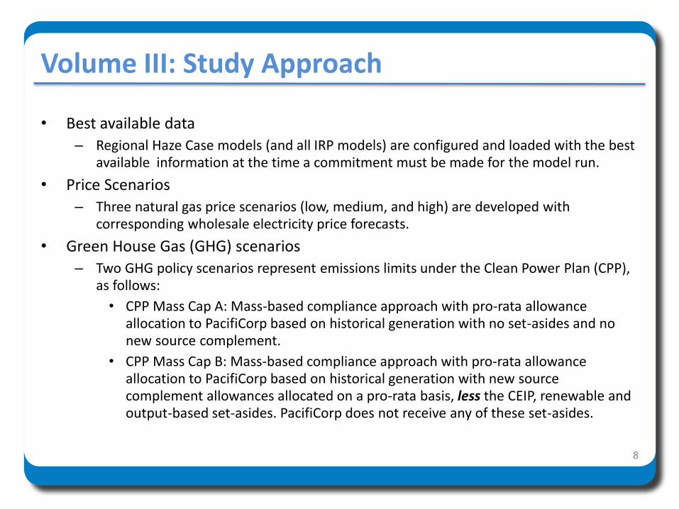
• Best available data
– Regional Haze Case models (and all IRP models) are configured and loaded with the best available information at the time a commitment must be made for the model run.
• Price Scenarios
– Three natural gas price scenarios (low, medium, and high) are developed with corresponding wholesale electricity price forecasts.
• Green House Gas (GHG) scenarios
– Two GHG policy scenarios represent emissions limits under the Clean Power Plan (CPP), as follows:
• CPP Mass Cap A: Mass-based compliance approach with pro-rata allowance allocation to PacifiCorp based on historical generation with no set-asides and no new source complement.
• CPP Mass Cap B: Mass-based compliance approach with pro-rata allowance allocation to PacifiCorp based on historical generation with new source complement allowances allocated on a pro-rata basis, less the CEIP, renewable and output-based set-asides. PacifiCorp does not receive any of these set-asides.
8
Volume III: Study Approach, continued
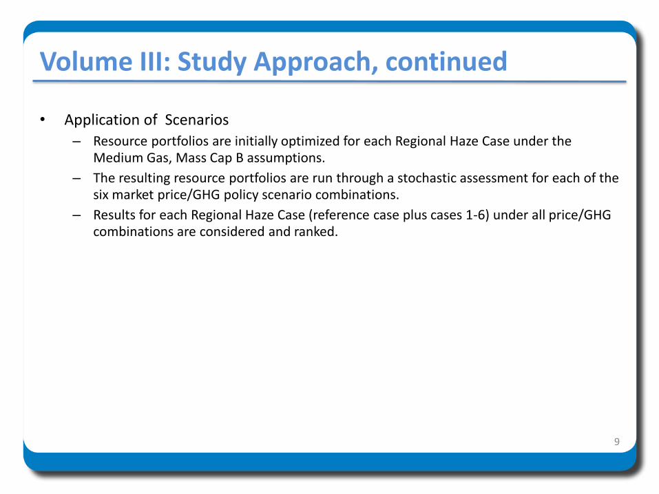
• Application of Scenarios
– Resource portfolios are initially optimized for each Regional Haze Case under the Medium Gas, Mass Cap B assumptions.
– The resulting resource portfolios are run through a stochastic assessment for each of the six market price/GHG policy scenario combinations.
– Results for each Regional Haze Case (reference case plus cases 1-6) under all price/GHG combinations are considered and ranked.
9

2017 IRP Price Scenarios
10
ScenarioClean Power Plan (CPP)
CaseCPP Attributes Natural Gas Power
10-2016 OFPC
CPP(b) BaseU.S. WECC* Mass Cap B total
allocation cap
New Source Complement
included; generic combined
cycles subject to constraint.
10-2016 OFPC (72-months
market; 12-months blend;
followed by base gas per
Expert 2)
10-2016 OFPC (72-months
market; 12-months blend;
followed by fundamentals
per Aurora®)
CPP(b) LowU.S. WECC* Mass Cap B total
allocation cap
New Source Complement
included; generic combined
cycles subject to constraint.
Low gas price per Expert 2Fundamental price forecast
per Aurora®
CPP(b) HighU.S. WECC* Mass Cap B total
allocation cap
New Source Complement
included; generic combined
cycles subject to constraint.
Adjusted high gas price per
Expert 2
Fundamental price forecast
per Aurora®
CPP(a) BaseU.S. WECC* Mass Cap A total
allocation cap
No New Source Complement;
generic combined cycles not
subject to constraint.
Base gas price per Expert 2Fundamental price forecast
per Aurora®
CPP(a) LowU.S. WECC* Mass Cap A total
allocation cap
No New Source Complement;
generic combined cycles not
subject to constraint
Low gas price per Expert 2Fundamental price forecast
per Aurora®
CPP(a) HighU.S. WECC* Mass Cap A total
allocation cap
No New Source Complement;
generic combined cycles not
subject to constraint
Adjusted high gas price per
Expert 2
Fundamental price forecast
per Aurora®
OFPC – Official Forward Price Curve; * California is modeled using a CO2 tax as a proxy for its cap-and-trade program established pursuant to
the California Global Warming Solutions Act of 2006. As such, it is not modeled as being subject to the CPP limits.

Henry Hub Natural Gas Prices
11
$0
$2
$4
$6
$8
$10
20
17
20
18
20
19
20
20
20
21
20
22
20
23
20
24
20
25
20
26
20
27
20
28
20
29
20
30
20
31
20
32
20
33
20
34
20
35
20
36
No
min
al $
/MM
Btu
Henry Hub
2017_IRP_Base (10.12.16 OFPC) 2017_IRP_High 2017_IRP_Low

2017Integrated Resource Plan
System Optimizer (SO) Modeling and Results

Volume III: System Optimizer PVRR
• Based upon the System Optimizer PVRR, Regional Haze Cases 1 and 5 provide the lowest net system costs, which are notably lower than the system costs from all other Cases (medium natural gas prices, mass cap B).
• When enabling endogenous early retirements (Regional Haze Case 6), net system costs are reduced relative to the Reference Case, but net costs are higher relative to other Regional Haze compliance Cases that reflect a range of potential negotiated compliance alternatives.
– Jim Bridger 2 retires year-end 2021
– SCRs installed on Hunter 1 & 2, Huntington 1 & 2, and Jim Bridger 1 13
15.4 15.6 15.8 15.8 15.6 15.8 15.7
8.8 7.6 7.7 7.6 8.1 7.4 8.3
$0
$5
$10
$15
$20
$25
Reference RH1 RH2 RH3 RH4 RH5 RH6
PV
RR
$ B
illio
n
System Optimizer PVRR System Costs
Variable Cost Fixed Cost
0.0 (1.1) (0.7) (0.8) (0.6) (1.0) (0.2)
($1.2)
($1.0)
($0.8)
($0.6)
($0.4)
($0.2)
$0.0
Reference RH1 RH2 RH3 RH4 RH5 RH6
PV
RR
$ B
illio
n
System PVRR Change from Reference

Vol. III: Ref and RH-1 Resource Portfolios
• 667 MW of coal is converted to natural gas by 2025, and 2,027 MW of coal is converted to natural gas or retired by 2036.
• 300 MW of renewables added in 2021, rising to 2,350 MW by 2036.
• 200 MW of natural gas peaking resource added in 2032.
• FOTs average 907 MW through 2020, 747 MW from 2021-2025, and 1,810 MW beyond 2025.
• 1,099 MW of incremental DSM by 2025, rising to 2,399 MW by 2036
14
(3) (2) (1)
- 1 2 3 4 5 6 7 8 9
20
17
20
18
20
19
20
20
20
21
20
22
20
23
20
24
20
25
20
26
20
27
20
28
20
29
20
30
20
31
20
32
20
33
20
34
20
35
20
36
GW
Cumulative Nameplate Capacity (Ref)
DSM FOTs Gas
Renewable Gas Conversion Other
Early Retirement End of Life Retirement
(4) (3) (2) (1)
- 1 2 3 4 5 6 7 8 9
20
17
20
18
20
19
20
20
20
21
20
22
20
23
20
24
20
25
20
26
20
27
20
28
20
29
20
30
20
31
20
32
20
33
20
34
20
35
20
36
GW
Cumulative Nameplate Capacity (RH-1)
DSM FOTs GasRenewable Gas Conversion OtherEarly Retirement End of Life Retirement
• 667 MW of coal is retired by 2025, and 2,740 MW of coal is retired by 2036.
• 300 MW of renewables added in 2021, rising to 1,554 MW by 2036.
• 200 MW of natural gas peaking resource and a 436 MW CCCT is added in 2030; CCCT capacity rises to 1,390 MW by 2036.
• FOTs average 1,037 MW through 2025, and 1,925 MW beyond 2025.
• 1,136 MW of incremental DSM by 2025, rising to 2,460 MW by 2036

Vol. III: RH-2 and RH-3 Resource Portfolios
• 1,103 MW of coal is converted to natural gas or retired by 2025; 3,428 MW retired by 2036.
• 300 MW of renewables added in 2021, rising to 2,076 MW by 2036.
• 436 MW of CCCT capacity is added in 2029, rising to 1,778 MW by 2036; 400 MW of natural gas peaking resource added in 2032.
• FOTs average 905 MW through 2020, 1,130 MW from 2021-2025, and 1,883 MW beyond 2025.
• 1,130 MW of incremental DSM by 2025, rising to 2,440 MW by 2036.
15
• 667 MW of coal is retired by 2025, rising to 2,740 MW by 2036.
• 235 MW of renewables added in 2021, rising to 2,338 MW by 2036.
• 436 MW of CCCT capacity is added in 2029, with an additional 477 MW resource added in 2030; 200 MW of natural gas peaking resource is added in 2029, rising to 600 MW by 2036.
• FOTs average 1,061 MW through 2025, and 1,839 MW beyond 2025.
• 1,157 MW of incremental DSM by 2025, rising to 2,496 MW by 2036
(5) (4) (3) (2) (1)
- 1 2 3 4 5 6 7 8 9
10
20
17
20
18
20
19
20
20
20
21
20
22
20
23
20
24
20
25
20
26
20
27
20
28
20
29
20
30
20
31
20
32
20
33
20
34
20
35
20
36
GW
Cumulative Nameplate Capacity (RH-2)
DSM FOTs GasRenewable Gas Conversion OtherEarly Retirement End of Life Retirement
(4) (3) (2) (1)
- 1 2 3 4 5 6 7 8 9
10
20
17
20
18
20
19
20
20
20
21
20
22
20
23
20
24
20
25
20
26
20
27
20
28
20
29
20
30
20
31
20
32
20
33
20
34
20
35
20
36
GW
Cumulative Nameplate Capacity (RH-3)
DSM FOTs GasRenewable Gas Conversion OtherEarly Retirement End of Life Retirement
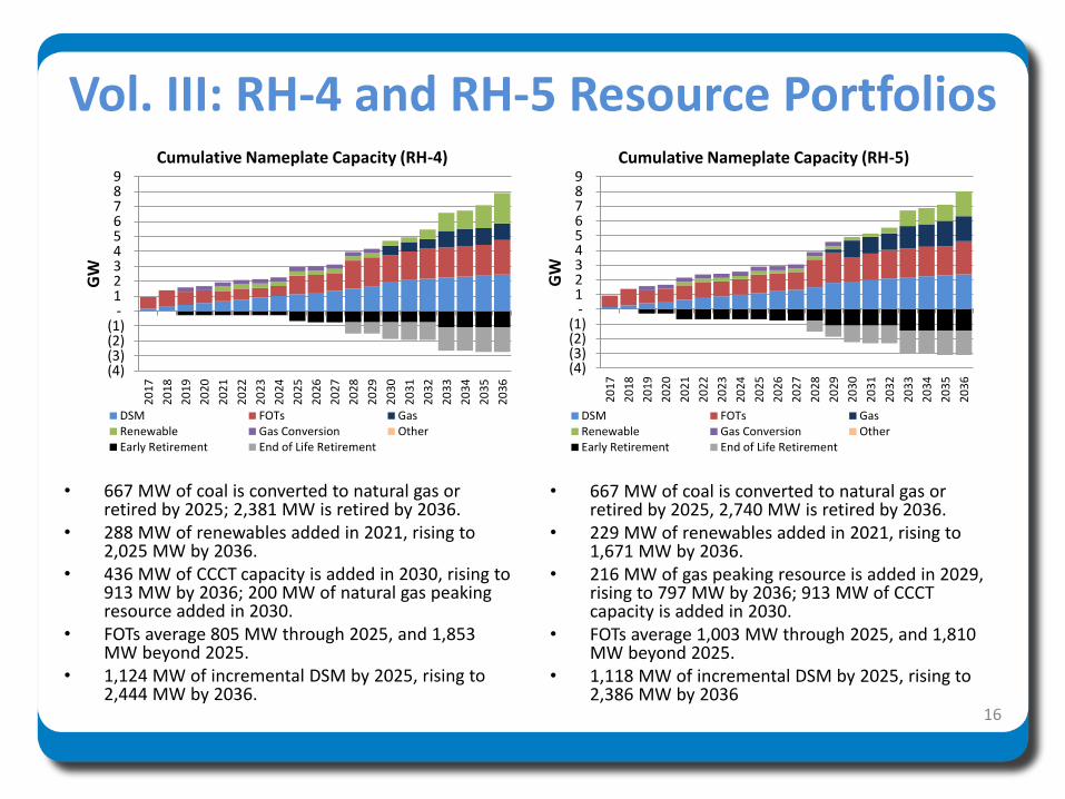
Vol. III: RH-4 and RH-5 Resource Portfolios
• 667 MW of coal is converted to natural gas or retired by 2025; 2,381 MW is retired by 2036.
• 288 MW of renewables added in 2021, rising to 2,025 MW by 2036.
• 436 MW of CCCT capacity is added in 2030, rising to 913 MW by 2036; 200 MW of natural gas peaking resource added in 2030.
• FOTs average 805 MW through 2025, and 1,853 MW beyond 2025.
• 1,124 MW of incremental DSM by 2025, rising to 2,444 MW by 2036.
16
• 667 MW of coal is converted to natural gas or retired by 2025, 2,740 MW is retired by 2036.
• 229 MW of renewables added in 2021, rising to 1,671 MW by 2036.
• 216 MW of gas peaking resource is added in 2029, rising to 797 MW by 2036; 913 MW of CCCT capacity is added in 2030.
• FOTs average 1,003 MW through 2025, and 1,810 MW beyond 2025.
• 1,118 MW of incremental DSM by 2025, rising to 2,386 MW by 2036
(4) (3) (2) (1)
- 1 2 3 4 5 6 7 8 9
20
17
20
18
20
19
20
20
20
21
20
22
20
23
20
24
20
25
20
26
20
27
20
28
20
29
20
30
20
31
20
32
20
33
20
34
20
35
20
36
GW
Cumulative Nameplate Capacity (RH-4)
DSM FOTs GasRenewable Gas Conversion OtherEarly Retirement End of Life Retirement
(4) (3) (2) (1)
- 1 2 3 4 5 6 7 8 9
20
17
20
18
20
19
20
20
20
21
20
22
20
23
20
24
20
25
20
26
20
27
20
28
20
29
20
30
20
31
20
32
20
33
20
34
20
35
20
36
GW
Cumulative Nameplate Capacity (RH-5)
DSM FOTs GasRenewable Gas Conversion OtherEarly Retirement End of Life Retirement
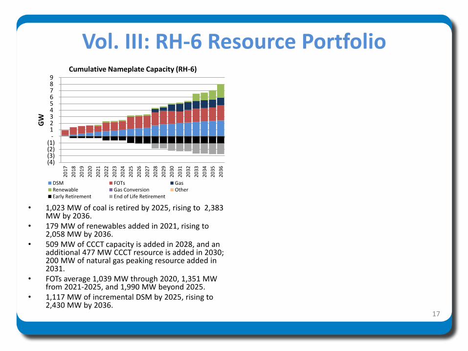
Vol. III: RH-6 Resource Portfolio
• 1,023 MW of coal is retired by 2025, rising to 2,383 MW by 2036.
• 179 MW of renewables added in 2021, rising to 2,058 MW by 2036.
• 509 MW of CCCT capacity is added in 2028, and an additional 477 MW CCCT resource is added in 2030; 200 MW of natural gas peaking resource added in 2031.
• FOTs average 1,039 MW through 2020, 1,351 MW from 2021-2025, and 1,990 MW beyond 2025.
• 1,117 MW of incremental DSM by 2025, rising to 2,430 MW by 2036.
17
(4) (3) (2) (1)
- 1 2 3 4 5 6 7 8 9
20
17
20
18
20
19
20
20
20
21
20
22
20
23
20
24
20
25
20
26
20
27
20
28
20
29
20
30
20
31
20
32
20
33
20
34
20
35
20
36
GW
Cumulative Nameplate Capacity (RH-6)
DSM FOTs GasRenewable Gas Conversion OtherEarly Retirement End of Life Retirement

2017Integrated Resource Plan
Planning and Risk (PaR) Modeling and Results

Planning and Risk (PaR) Modeling Features• PaR model results are used develop portfolio ranking metrics.
– Mean PVRR, upper tail PVRR, risk-adjusted PVRR
– Mean Energy Not Served (ENS), upper tail ENS
– Emissions
• 2017 IRP PaR Configuration – PaR calculates 50-iterations for 12 sample weeks.
– Each iteration applies varying stochastic shocks to loads, gas and power prices, thermal outages and hydro.
– Each sample week represents a one-month period.
– Sample weeks capture the peak load week for each month.
– 50 iterations provide practical performance and are sufficient to ensure convergence of stochastic draws.
– CO2 shadow prices from System Optimizer are input into PaR to reduce thermal dispatch, as required, and achieve mass cap emission limits.
– The resulting CO2 costs reported by PaR represent the opportunity cost of the CPP, but are not real expenses, and thus they are removed in the final PVRR reporting.
19

CPP Modeling in PaR• PaR models emissions limits are enforced by a CO2 shadow price,
which is an output from System Optimizer.– The CO2 shadow price represents the incremental system cost, expressed in $/ton of
affected emissions, of meeting CPP mass cap assumptions.
– This represents a modeling improvement relative to the 2015 IRP, where a shadow price could not be determined with System Optimizer.
• CPP serves as the emissions cap for states other than WA and AZ.– Exceedances under CPP are rare(<6% of iterations among all cases across and price
curve scenarios).
• Washington Clean Air Rule (CAR) limit applies to WA emissions. – WA CAR exceedances occur in greater frequency and volume relative to the CPP;
however, CAR allows for use of emission reduction units (ERUs).
– In the absence of an ERU market, RECs convert to ERUs.
20
CO2 Shadow Prices (Low to High Range Among Regional Haze Cases)
21
$0
$10
$20
$30
$40
$50
20
17
20
19
20
21
20
23
20
25
20
27
20
29
20
31
20
33
20
35
20
18
20
20
20
22
20
24
20
26
20
28
20
30
20
32
20
34
20
36
20
17
20
19
20
21
20
23
20
25
20
27
20
29
20
31
20
33
20
35
Low Gas Medium Gas High Gas
$/t
on
Mass Cap A
Low High
$0
$10
$20
$30
$40
$50
20
17
20
19
20
21
20
23
20
25
20
27
20
29
20
31
20
33
20
35
20
18
20
20
20
22
20
24
20
26
20
28
20
30
20
32
20
34
20
36
20
17
20
19
20
21
20
23
20
25
20
27
20
29
20
31
20
33
20
35
Low Gas Medium Gas High Gas
$/t
on
Mass Cap B
Low High
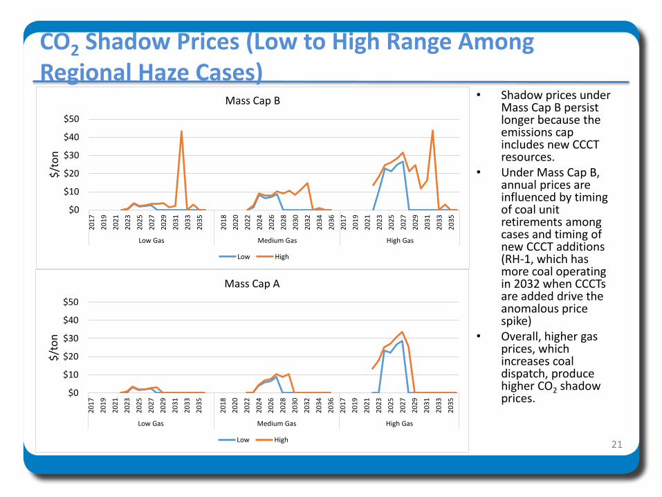
• Shadow prices under Mass Cap B persist longer because the emissions cap includes new CCCT resources.
• Under Mass Cap B, annual prices are influenced by timing of coal unit retirements among cases and timing of new CCCT additions (RH-1, which has more coal operating in 2032 when CCCTs are added drive the anomalous price spike)
• Overall, higher gas prices, which increases coal dispatch, produce higher CO2 shadow prices.

$23.6
$23.8
$24.0
$24.2
$24.4
$24.6
$24.8
$25.0
$23.3 $23.5 $23.7 $23.9 $24.1 $24.3 $24.5 $24.7
Up
per
Ta
il M
ean
PV
RR
($ b
illi
on
)
Stochastic Mean PVRR($ billion)
Medium Gas, Mass Cap B
Ref RH1 RH2 RH3 RH4 RH5 RH6
$22.8
$23.0
$23.2
$23.4
$23.6
$23.8
$24.0
$24.2
$24.4
$24.6
$22.5 $22.7 $22.9 $23.1 $23.3 $23.5 $23.7 $23.9 $24.1 $24.3
Up
per
Ta
il M
ean
PV
RR
($ b
illi
on
)
Stochastic Mean PVRR($ billion)
Low Gas, Mass Cap B
Ref RH1 RH2 RH3 RH4 RH5 RH6
$26.0
$26.2
$26.4
$26.6
$26.8
$27.0
$27.2
$27.4
$25.5 $25.7 $25.9 $26.1 $26.3 $26.5 $26.7 $26.9
Up
per
Ta
il M
ean
PV
RR
($ b
illi
on
)
Stochastic Mean PVRR($ billion)
High Gas, Mass Cap B
Ref RH1 RH2 RH3 RH4 RH5 RH6
Vol. III: PaR Scatter Plots - Mass Cap B with Fixed Cost
• With fixed costs included in the upper tail mean, which does not change among stochastic iterations, cost and risk are highly correlated.
• RH-5 is least cost, least risk under both medium and low natural gas price scenarios.
• RH-1 is least cost, least risk when high natural gas prices are assumed.
22

$23.6
$23.8
$24.0
$24.2
$24.4
$24.6
$24.8
$25.0
$23.2 $23.4 $23.6 $23.8 $24.0 $24.2 $24.4 $24.6 $24.8
Up
per
Ta
il M
ean
PV
RR
($ b
illi
on
)
Stoch
astic Mean PVRR($ billion)
Medium Gas, Mass Cap A
Ref RH1 RH2 RH3 RH4 RH5 RH6
$23.0
$23.2
$23.4
$23.6
$23.8
$24.0
$24.2
$24.4
$22.5 $22.7 $22.9 $23.1 $23.3 $23.5 $23.7 $23.9 $24.1
Up
per
Ta
il M
ean
PV
RR
($ b
illi
on
)
Stochastic Mean PVRR($ billion)
Low Gas, Mass Cap A
Ref RH1 RH2 RH3 RH4 RH5 RH6
$26.0
$26.2
$26.4
$26.6
$26.8
$27.0
$27.2
$27.4
$25.4 $25.6 $25.8 $26.0 $26.2 $26.4 $26.6 $26.8 $27.0
Up
per
Ta
il M
ean
PV
RR
($ b
illi
on
)
Stochastic Mean PVRR($ billion)
High Gas, Mass Cap A
Ref RH1 RH2 RH3 RH4 RH5 RH6
Vol. III: PaR Scatter Plots - Mass Cap A with Fixed Cost
• With fixed costs included in the upper tail mean, which does not change among stochastic iterations, cost and risk are highly correlated.
• RH-5 is least cost, least risk under both medium and low natural gas price scenarios.
• RH-1 is least cost, least risk when high natural gas prices are assumed.
• Distribution among cases is similar to Mass Cap B. 23

$16.0
$16.2
$16.4
$16.6
$23.2 $23.4 $23.6 $23.8 $24.0 $24.2 $24.4 $24.6 $24.8
Up
per
Ta
il M
ean
PV
RR
Les
s F
ixed
Co
sts
($ b
illi
on
)
Stochastic Mean PVRR($ billion)
Medium Gas, Mass Cap B
Ref RH1 RH2 RH3 RH4 RH5 RH6
$15.4
$15.6
$15.8
$22.6 $22.8 $23.0 $23.2 $23.4 $23.6 $23.8 $24.0 $24.2
Up
per
Ta
il M
ean
PV
RR
Les
s F
ixed
Co
sts
($ b
illi
on
)
Stochastic Mean PVRR($ billion)
Low Gas, Mass Cap B
Ref RH1 RH2 RH3 RH4 RH5 RH6
$18.0
$18.2
$18.4
$18.6
$18.8
$19.0
$19.2
$19.4
$25.7 $25.9 $26.1 $26.3 $26.5 $26.7 $26.9
Up
per
Ta
il M
ean
PV
RR
Les
s F
ixed
Co
sts
($ b
illi
on
)
Stochastic Mean PVRR($ billion)
High Gas, Mass Cap B
Ref RH1 RH2 RH3 RH4 RH5 RH6
Vol. III: PaR Scatter Plots - Mass Cap B, no Fixed Cost
• When fixed costs are removed from the upper tail mean, variable cost risk among portfolios is more apparent.
• RH-5 is least cost under both medium and low natural gas price scenarios.
• RH-1 is least cost, least risk when high natural gas prices are assumed. 24
$16.0
$16.2
$16.4
$16.6
$23.0 $23.2 $23.4 $23.6 $23.8 $24.0 $24.2 $24.4 $24.6 $24.8
Up
per
Ta
il M
ean
PV
RR
Les
s F
ixed
Co
sts
($ b
illi
on
)
Stochastic Mean PVRR($ billion)
Medium Gas, Mass Cap A
Ref RH1 RH2 RH3 RH4 RH5 RH6
$15.4
$15.6
$15.8
$16.0
$22.5 $22.7 $22.9 $23.1 $23.3 $23.5 $23.7 $23.9 $24.1
Up
per
Ta
il M
ean
PV
RR
Les
s F
ixed
Co
sts
($ b
illi
on
)
Stochastic Mean PVRR($ billion)
Low Gas, Mass Cap A
Ref RH1 RH2 RH3 RH4 RH5 RH6
$18.2
$18.4
$18.6
$18.8
$19.0
$19.2
$19.4
$19.6
$19.8
$20.0
$25.4 $25.6 $25.8 $26.0 $26.2 $26.4 $26.6 $26.8 $27.0
Up
per
Ta
il M
ean
PV
RR
Les
s F
ixed
Co
sts
($ b
illi
on
)
Stochastic Mean PVRR($ billion)
High Gas, Mass Cap A
Ref RH1 RH2 RH3 RH4 RH5 RH6
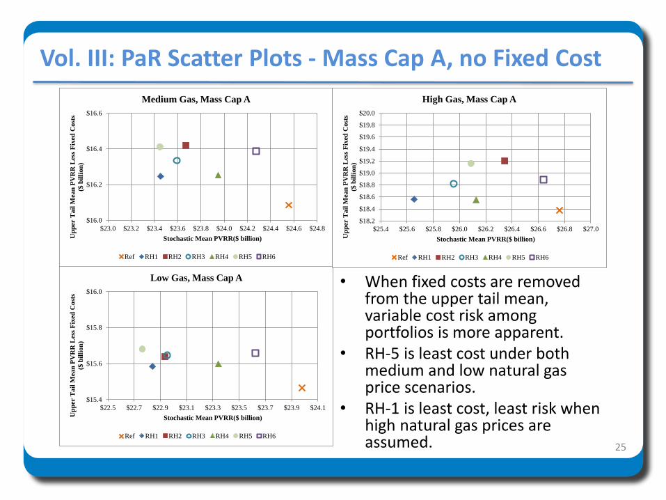
Vol. III: PaR Scatter Plots - Mass Cap A, no Fixed Cost
• When fixed costs are removed from the upper tail mean, variable cost risk among portfolios is more apparent.
• RH-5 is least cost under both medium and low natural gas price scenarios.
• RH-1 is least cost, least risk when high natural gas prices are assumed. 25

Vol. III: PaR Summary Rankings (All Scenarios)• Cases RH-1 and RH-5 perform best on a risk-adjusted PVRR basis--more
notable separation among the other cases• Energy not served (ENS) results are tightly grouped
– Cases RH-3 and RH-5 produce the lowest mean ENS – Cases RH-5 and RH-3 produce the lowest upper tail ENS
• Cases RH-2 and RH-5 produce the lowest CO2 emissions• With equal weighting among all metrics and scenarios, Cases RH-5 and RH-3
rank highest among all Regional Haze Cases.
26
Risk Adjusted CO2 Emissions Average
PVRR
($m)
Change
from
Lowest
Cost
Portfolio
($m) Rank
Average
Annual
ENS,
2017-
2036
(GWh)
Change
from
Lowest
ENS
Portfolio Rank
Average
Annual
ENS,
2017-
2036
(GWh)
Change
from
Lowest
ENS
Portfolio Rank
Total CO2
Emissions,
2017-2036
(Thousand
Tons)
Change
from
Lowest
Emission
Portfolio Rank Rank
Ref 26,395 $1,146 7 14.1 2.6 7 33.7 3.3 6 786,334 27,895 4 6
RH1 25,249 $0 1 11.9 0.4 4 31.5 1.1 5 789,172 30,732 6 4
RH2 25,544 $295 4 12.2 0.7 5 34.7 4.2 7 758,440 0 1 4
RH3 25,414 $165 3 11.5 0.0 1 30.6 0.1 2 778,734 20,294 3 2
RH4 25,757 $508 5 11.9 0.4 3 30.6 0.2 3 790,896 32,456 7 5
RH5 25,307 $58 2 11.7 0.3 2 30.4 0.0 1 773,115 14,676 2 2
RH6 26,111 $862 6 12.4 1.0 6 31.1 0.7 4 787,410 28,971 5 5
Case
ENS Upper Tail AverageENS Scenario Average
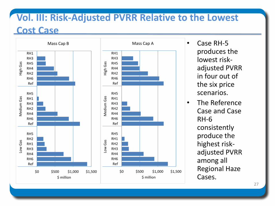
Vol. III: Risk-Adjusted PVRR Relative to the Lowest Cost Case
27
• Case RH-5 produces the lowest risk-adjusted PVRR in four out of the six price scenarios.
• The Reference Case and Case RH-6 consistently produce the highest risk-adjusted PVRR among all Regional Haze Cases.
$0 $500 $1,000 $1,500
Ref
RH6
RH4
RH3
RH1
RH2
RH5
Ref
RH6
RH4
RH2
RH3
RH1
RH5
Ref
RH6
RH2
RH4
RH5
RH3
RH1
Low
Gas
Med
ium
Gas
Hig
h G
as
$ million
Mass Cap B
$0 $500 $1,000 $1,500
Ref
RH6
RH4
RH3
RH2
RH1
RH5
Ref
RH6
RH4
RH2
RH3
RH1
RH5
Ref
RH6
RH2
RH4
RH5
RH3
RH1
Low
Gas
Med
ium
Gas
Hig
h G
as
$ million
Mass Cap A
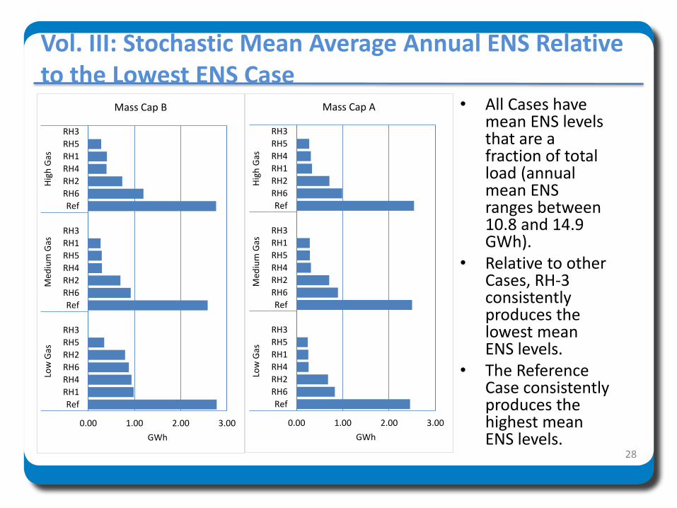
Vol. III: Stochastic Mean Average Annual ENS Relative to the Lowest ENS Case
28
0.00 1.00 2.00 3.00
Ref
RH1
RH4
RH6
RH2
RH5
RH3
Ref
RH6
RH2
RH4
RH5
RH1
RH3
Ref
RH6
RH2
RH4
RH1
RH5
RH3
Low
Gas
Med
ium
Gas
Hig
h G
as
GWh
Mass Cap B
0.00 1.00 2.00 3.00
Ref
RH6
RH2
RH4
RH1
RH5
RH3
Ref
RH6
RH2
RH4
RH5
RH1
RH3
Ref
RH6
RH2
RH1
RH4
RH5
RH3
Low
Gas
Med
ium
Gas
Hig
h G
as
GWh
Mass Cap A • All Cases have mean ENS levels that are a fraction of total load (annual mean ENS ranges between 10.8 and 14.9 GWh).
• Relative to other Cases, RH-3 consistently produces the lowest mean ENS levels.
• The Reference Case consistently produces the highest mean ENS levels.

29
• All Cases have upper tail ENS levels that are a fraction of total load (upper tail annual ENS ranges between 30.1 and 35.8 GWh).
• Relative to other Cases, RH-5 and RH-4 consistently produce the lowest upper tail ENS levels.
• RH-2 and the Reference Case consistently produces the highest upper tail ENS levels.
0.00 2.00 4.00 6.00
RH2
Ref
RH1
RH4
RH6
RH3
RH5
RH2
Ref
RH1
RH6
RH3
RH5
RH4
RH2
Ref
RH1
RH6
RH4
RH3
RH5
Low
Gas
Med
ium
Gas
Hig
h G
as
GWh
Mass Cap B
0.00 1.00 2.00 3.00 4.00 5.00
RH2
Ref
RH1
RH6
RH3
RH4
RH5
RH2
Ref
RH1
RH6
RH4
RH3
RH5
RH2
Ref
RH1
RH6
RH3
RH5
RH4
Low
Gas
Med
ium
Gas
Hig
h G
as
GWh
Mass Cap A
Vol. III: Upper Tail Average Annual ENS Relative to the Lowest ENS Case

30
• Case RH-2, with earliest coal retirements, consistently yields the lowest emissions among all Regional Haze Cases .
• Case RH-5 yields relatively low emissions relative to other cases among most scenarios.
• Case RH-4, with latest coal retirements, consistently yields emissions that are higher than other Regional Haze cases.
Vol. III: Total CO2 Emissions Relative to the Lowest Emission Case
0 10,000 20,000 30,000 40,000
RH6
RH5
RH4
RH1
Ref
RH3
RH2
RH6
RH4
Ref
RH1
RH3
RH5
RH2
RH6
RH4
RH1
Ref
RH3
RH5
RH2
Low
Gas
Med
ium
Gas
Hig
h G
as
Thousand Tons
Mass Cap B
0 10,000 20,000 30,000 40,000 50,000
RH4
RH1
Ref
RH6
RH3
RH5
RH2
RH4
RH1
Ref
RH6
RH3
RH5
RH2
RH4
RH1
RH6
Ref
RH3
RH5
RH2
Low
Gas
Med
ium
Gas
Hig
h G
as
Thousand Tons
Mass Cap A
Conclusion• The Company has selected Case RH-5 as the top performing Regional Haze Case.• Case RH-5 produces the lowest risk-adjusted PVRR in 4 out of 6 price scenarios and is
among the top 3 Cases in the other 2 price scenarios.• Case RH-5 is consistently among the top performing portfolios when ranked on mean
and upper tail ENS.• Case RH-5 is among the top 2 portfolios when ranked on CO2 emissions in 5 out of 6
price scenarios.– Case RH-5 produces a notably lower risk adjusted PVRR than the top performing emissions portfolio
(Case RH-2).– Emission differences between cases are closely bunched in the remaining price scenario.
• Case RH-5 produces a low PVRR relative to other Regional Haze Cases based on the PVRR from System Optimizer.
– Case RH-5 and RH-1 are very close when evaluating PVRR from System Optimizer, but Case RH-1 only exhibits the lowest risk-adjusted PVRR in the high price scenarios.
• Case RH-5 is a blend of Cases RH-1, RH-2, and RH-3, and is a balanced representation of potential Regional Haze outcomes.
• Individual unit outcomes under any Regional Haze compliance case will ultimately be determined by ongoing rulemaking, results of litigation, and future negotiations with state and federal agencies, partner plant owners, and other vested stakeholders. No individual unit commitments are being made at this time.
• Additional Core Case and Sensitivity Case studies will be completed before the preferred portfolio is selected.
31

2017Integrated Resource Plan
Flexible Capacity
Reserve Requirements Study

Flex Capacity Reserve Requirements Study Hourly Regulation Reserve Forecast Goals:
– Compliance with standard BAL-001-2
– Minimize regulation reserve held
– Compliance with EIM tests and hourly scheduling timelines
Methodology was described at IRP Public Meeting 4 (9/23/16).– Draft study online at https://www.oasis.oati.com/ppw/index.html
– Navigate [Documents > PacifiCorp OASIS Tariff/Company Information > OATT Pricing > Ancillary Services]
Today’s Presentation:– Solar Reserve Requirements
– Combined Portfolio Requirements
– Incremental Cost Results: Regulation Reserve & System Balancing
33

0
200
400
600
800
1000
Cu
mu
lati
ve S
ola
r C
apac
ity
(MW
)
East
East - Projected
West
West - Projected
Pavant I
Red Hills
Available 5-min data
Solar Capacity and Data vs Time
34
• Solar capacity is increasing in both PACE and PACW.
• Limited five minute actual data available:Pavant I (50MW) Red Hills (80MW)
• EIM deviations in this time frame may be overstated as DNV-GL had not fully implemented its forecasting process.
• Proxy solar base schedules (forecasts) are needed to determine deviations and reserve requirements.
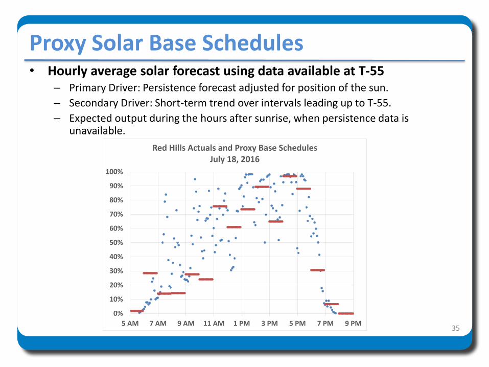
Proxy Solar Base Schedules• Hourly average solar forecast using data available at T-55
– Primary Driver: Persistence forecast adjusted for position of the sun.
– Secondary Driver: Short-term trend over intervals leading up to T-55.
– Expected output during the hours after sunrise, when persistence data is unavailable.
35
0%
10%
20%
30%
40%
50%
60%
70%
80%
90%
100%
5 AM 7 AM 9 AM 11 AM 1 PM 3 PM 5 PM 7 PM 9 PM
Red Hills Actuals and Proxy Base SchedulesJuly 18, 2016

y = -0.0682x - 0.0049
-40%
-20%
0%
20%
40%
0% 20% 40% 60% 80% 100%
Div
ers
ity
(Co
mb
ine
d B
AA
L vs
Ind
ep.)
Independent BAAL Requirements
Diversity
Linear (Diversity)Exacerbating:Higher BAAL
Offsetting:Lower BAAL
0%
20%
40%
60%
80%
100%
0% 20% 40% 60% 80% 100%
Exce
ed
ance
Pro
bab
ility
BAAL Requirement
Proxy Red HillsProxy Pavant 1
Solar Deviations• Deviations are the difference between the base schedule and actual output.• BAL-001-2: Requirement 2:
“Each Balancing Authority shall operate such that its clock-minute average of Reporting ACE does not exceed its clock-minute Balancing Authority ACE Limit (BAAL) for more than 30 consecutive clock-minutes…”
• Independent BAAL regulation requirements for Red Hills and Pavant I are on the left.• Combining Red Hills and Pavant I can result in either higher or lower BAAL regulation
requirements due to intra-hour timing differences—the difference is referred to as “diversity”.• Deviations offset more often than they exacerbate, with a slightly greater diversity when
individual requirements are higher.
36

Solar Locations• All solar facilities on PacifiCorp system are in southern and central Oregon, and
southeastern Utah. Facilities are also clustered within these areas.
• Five clusters were identified in Utah, while three were identified in Oregon.
• One of the Oregon clusters is relatively dispersed, and is treated as two independent clusters.
37
So
uth
easte
rn U
tah
So
uth
/Cen
tral O
reg
on Bend
Klamath 1Medford
Pavant
EnterpriseFiddler’s
Canyon
Red
Hills
Escalante
Klamath 2
30 miles 30 miles

West Clusters Base Incr. Solar 1 Incr. Solar 2Bend 50 +31 +6Medford 20 +12 +2Klamath 1 47 +29 +6Klamath 2 47 +29 +6New Cluster 1 +80Total 163 263 363
% Change vs Base 61% 123%
East Clusters Base Incr. Solar 1 Incr. Solar 2Enterprise 83 +17 +17Fiddler’s Canyon 311 +62 +62Escalante 257 +51 +51Red Hills 83 +17 +17Pavant 120 +24 +24New Cluster 1 +229New Cluster 2 +229Total 855 1255 1655
% Change vs Base 47% 94%
38
Solar Penetration ScenariosBase: 2017 Expected Solar CapacityIncremental Solar 1: 2017 +400 MW East +100 MW WestIncremental Solar 2: 2017 +800 MW East +200 MW West
Solar Capacity Additions (MW):

39
Combined Solar Portfolio Data• Red Hills and Pavant have proxy BAAL requirements and diversity based on actual
generation.• BAAL requirements and diversity for other clusters are unknown.
For each interval, assumed BAAL requirements are assigned randomly from a distribution containing the Red Hills and Pavant results.
Diversity is partly a linear function of the BAAL requirement. Variation around that linear function is assigned randomly from a distribution
containing the Red Hills/Pavant diversity results. Because requirements are bounded by zero and maximum solar output, the overall
hourly shape is scaled back to align with the Red Hills and Pavant results.
To reiterate:Data available for two clusters:
• Pavant I: 50 MW• Red Hills: 80 MW
Data developed for:• East Base: 855 MW, 5 clusters• East+New 1: 1,255 MW, 6 clusters• East+New 2: 1,655 MW, 7 clusters• West Base: 163 MW, 4 clusters• West+New 1: 263 MW, 4 clusters• West+New 2: 363 MW, 5 clusters

0%
10%
20%
30%
40%
50%
60%
70%
80%
90%
100%
0% 10% 20% 30% 40% 50% 60% 70% 80% 90% 100%
Exce
edan
ce P
roba
bilit
y
BAAL Requirement
Red Hills EIM Pavant I EIM
Proxy Red Hills/Pavant Existing EIM (Equal Weighting)
Proxy East Base
EIM vs Proxy Results
40
Existing EIM (as of 4/1/16)
Group Plant MW Weighting
Fiddlers Fiddler's Canyon 1-3 9 20%
Enterprise Beryl Solar 3 20%
Escalante Granite Peak 3 20%
Red Hills Utah Red Hills Solar 80 20%
Pavant Utah Pavant Solar 50 20%
Deviations are expressed as c.f., then averaged.
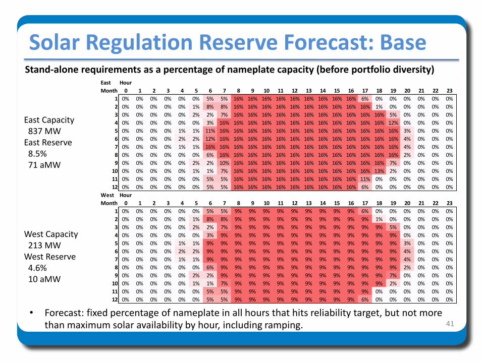
West Capacity213 MW
West Reserve4.6%10 aMW
41
Solar Regulation Reserve Forecast: BaseStand-alone requirements as a percentage of nameplate capacity (before portfolio diversity)
• Forecast: fixed percentage of nameplate in all hours that hits reliability target, but not more than maximum solar availability by hour, including ramping.
East Capacity837 MW
East Reserve8.5%71 aMW
East Hour
Month 0 1 2 3 4 5 6 7 8 9 10 11 12 13 14 15 16 17 18 19 20 21 22 23
1 0% 0% 0% 0% 0% 0% 5% 5% 16% 16% 16% 16% 16% 16% 16% 16% 16% 6% 0% 0% 0% 0% 0% 0%
2 0% 0% 0% 0% 0% 1% 8% 8% 16% 16% 16% 16% 16% 16% 16% 16% 16% 16% 1% 0% 0% 0% 0% 0%
3 0% 0% 0% 0% 0% 2% 2% 7% 16% 16% 16% 16% 16% 16% 16% 16% 16% 16% 16% 5% 0% 0% 0% 0%
4 0% 0% 0% 0% 0% 0% 3% 16% 16% 16% 16% 16% 16% 16% 16% 16% 16% 16% 16% 12% 0% 0% 0% 0%
5 0% 0% 0% 0% 1% 1% 11% 16% 16% 16% 16% 16% 16% 16% 16% 16% 16% 16% 16% 16% 3% 0% 0% 0%
6 0% 0% 0% 0% 2% 2% 12% 16% 16% 16% 16% 16% 16% 16% 16% 16% 16% 16% 16% 16% 4% 0% 0% 0%
7 0% 0% 0% 0% 1% 1% 16% 16% 16% 16% 16% 16% 16% 16% 16% 16% 16% 16% 16% 16% 4% 0% 0% 0%
8 0% 0% 0% 0% 0% 0% 6% 16% 16% 16% 16% 16% 16% 16% 16% 16% 16% 16% 16% 16% 2% 0% 0% 0%
9 0% 0% 0% 0% 0% 2% 2% 10% 16% 16% 16% 16% 16% 16% 16% 16% 16% 16% 16% 7% 0% 0% 0% 0%
10 0% 0% 0% 0% 0% 1% 1% 7% 16% 16% 16% 16% 16% 16% 16% 16% 16% 16% 13% 2% 0% 0% 0% 0%
11 0% 0% 0% 0% 0% 0% 5% 5% 16% 16% 16% 16% 16% 16% 16% 16% 16% 11% 0% 0% 0% 0% 0% 0%
12 0% 0% 0% 0% 0% 0% 5% 5% 16% 16% 16% 16% 16% 16% 16% 16% 16% 6% 0% 0% 0% 0% 0% 0%
West Hour
Month 0 1 2 3 4 5 6 7 8 9 10 11 12 13 14 15 16 17 18 19 20 21 22 23
1 0% 0% 0% 0% 0% 0% 5% 5% 9% 9% 9% 9% 9% 9% 9% 9% 9% 6% 0% 0% 0% 0% 0% 0%
2 0% 0% 0% 0% 0% 1% 8% 8% 9% 9% 9% 9% 9% 9% 9% 9% 9% 9% 1% 0% 0% 0% 0% 0%
3 0% 0% 0% 0% 0% 2% 2% 7% 9% 9% 9% 9% 9% 9% 9% 9% 9% 9% 9% 5% 0% 0% 0% 0%
4 0% 0% 0% 0% 0% 0% 3% 9% 9% 9% 9% 9% 9% 9% 9% 9% 9% 9% 9% 9% 0% 0% 0% 0%
5 0% 0% 0% 0% 1% 1% 9% 9% 9% 9% 9% 9% 9% 9% 9% 9% 9% 9% 9% 9% 3% 0% 0% 0%
6 0% 0% 0% 0% 2% 2% 9% 9% 9% 9% 9% 9% 9% 9% 9% 9% 9% 9% 9% 9% 4% 0% 0% 0%
7 0% 0% 0% 0% 1% 1% 9% 9% 9% 9% 9% 9% 9% 9% 9% 9% 9% 9% 9% 9% 4% 0% 0% 0%
8 0% 0% 0% 0% 0% 0% 6% 9% 9% 9% 9% 9% 9% 9% 9% 9% 9% 9% 9% 9% 2% 0% 0% 0%
9 0% 0% 0% 0% 0% 2% 2% 9% 9% 9% 9% 9% 9% 9% 9% 9% 9% 9% 9% 7% 0% 0% 0% 0%
10 0% 0% 0% 0% 0% 1% 1% 7% 9% 9% 9% 9% 9% 9% 9% 9% 9% 9% 9% 2% 0% 0% 0% 0%
11 0% 0% 0% 0% 0% 0% 5% 5% 9% 9% 9% 9% 9% 9% 9% 9% 9% 9% 0% 0% 0% 0% 0% 0%
12 0% 0% 0% 0% 0% 0% 5% 5% 9% 9% 9% 9% 9% 9% 9% 9% 9% 6% 0% 0% 0% 0% 0% 0%

42
Incremental Solar Regulation Reserve Cap
•More diverse solar resources have lower requirements. The incremental effect declines as diversity increases.• Spreading the fixed allowable BAAL variation across more capacity increases requirements. The incremental effect increases as capacity increases.• PACE is modeled using a 3rd order polynomial.• PACW is modeled using two linear extrapolations.
Base Incr. Solar 1 Incr. Solar 2
Base
Red Hills and
Pavant Only
•The fixed percentage of nameplate in the reserve requirement is a function of solar capacity.

43
Portfolio Diversity Effects• A single pool of regulation reserve is held to cover deviations by load, wind, solar, and other
non-dispatchable generation.
• Simultaneous large deviations by all classes are unlikely – this is portfolio diversity.
• In the absence of solar:• Incremental wind generation was calculated to have reserve requirements of 6.1%.• System diversity, including EIM benefits, reduces reserve requirements by 37.51%.• The trend is assumed to be linear - a small increase in diversity as the reserve
requirement of the existing classes grows.
• Adding a new class should create incremental diversity, but the first new source of diversity has more benefit than the second, which has more benefit than the third.
• Incremental solar diversity of up to 20% of solar requirements is assumed to be achieved when classes are similarly sized, and is proportional to that share up to that point.
• Base Scenario Diversity:37.6% of 998 MW: based on a linear trend without solar
+ 6.5% of 81 MW: incremental diversity from solar= 38.2% of 998 MW: base scenario result

Portfolio Allocation (Class Average Reserve as % of Nameplate)
Case Load Wind Non-VER Solar
No solar 2.80% 9.01% 2.39% 0.00%
Base 2.77% 8.94% 2.37% 4.61%
Incr Wind 2.77% 8.69% 2.37% 4.61%
Incr Solar 1 2.76% 8.88% 2.36% 4.49%
Incr Solar 2 2.74% 8.81% 2.34% 4.53%
A B C D
Case
Wind
Capacity
Solar
Capacity
Regulation
Req Diversity
1 No solar 2757.4 0.0 572.6 37.5% Incr % of Nameplate
2 Base 2757.4 1050.5 616.7 38.2% Base vs No Solar 4.2% Solar =(C2-C1)/(B2-B1)
3 Incr Wind 3007.4 1050.5 631.2 38.3% Incr Wind vs Base 5.8% Wind =(C3-C2)/(A3-A2)
4 Incr Solar 1 2757.4 1550.5 634.5 38.6% Solar1 vs Base 3.6% Solar =(C4-C2)/(B4-B2)
5 Incr Solar 2 2757.4 2050.5 653.3 39.2% Solar2 vs Solar1 3.7% Solar =(C5-C4)/(B5-B4)
44
Regulation Requirement Results• Hourly regulation requirements for PACE and PACW are calculated as a function of:
• Wind and solar nameplate capacity.• Wind output and month/hour as a proxy for expected solar output.• Static hourly values for load and non-VER generation.
• Diversity is calculated dynamically based on the inputs above.

45
Comparison to Prior Results
• On a percentage basis, requirements generally decrease as more components are added, because of diversity.
• The 2012 and 2014 Wind Integration Studies calculated the regulation reserve requirement for load only, then the incremental requirement for the entire wind fleet, allocating all diversity to wind.
• The 2016 Flexible Capacity Requirement Study calculates the regulation reserve requirement for the 2015 resource mix, allocating the diversity to all components.
• As compared to prior studies, diversity allocation decreases the load requirement and increases the wind requirement, the changes in standards and methodology notwithstanding.
• Incremental requirements for wind and solar are lower than the average requirements in the base case, but will call on higher cost resources.
Study Load Wind Non-VER Solar Method
2012 WIS 3.90% 8.70% - - Load -> Incr Wind
2014 WIS 4.00% 8.10% - - Load -> Incr Wind
2014 WIS 4.40% 7.30% - - Load -> Incr Wind
2016 Flex 2.77% 8.94% 2.37% 4.61% Portfolio Diversity (Base)
2016 Flex - 5.78% - - Base -> Incr Wind
2016 Flex - - - 3.56% Base -> Incr Solar 1
2016 Flex - - - 3.66% Incr Solar 1 -> Incr Solar 2

46
Regulation Reserve Cost (2016$)
• While incremental reserve costs generally increase with volume, the 500 MW solar study (S1) had a slightly higher cost than S2, likely due to lower transmission congestion. For simplicity, the average S2 results are being applied in the IRP.
• The difference in reserve costs for wind and solar resource reflects timing differences. Per MWh of generation, the wind obligation is 16% higher than the solar obligation.
Regulation Reserve PaR Scenarios
# Scenario Resources
B.1 Base No Reserve Jan. 1, 2017 levels of wind and solar None
B.2 Base With Reserve Jan. 1, 2017 levels of wind and solar Requirements for 1/1/17 wind and solar
W.1 Incremental Wind, Base Reserve Study B.2 + 250MW of wind capacity Requirements for 1/1/17 wind and solar
W.2 Incremental Wind+Reserve Study B.2 + 250MW of wind capacity Study B.2 + Reserve for additional 250MW wind capacity
S1.1 Incremental Solar, Base Reserve Study B.2 + 500MW of solar capacity Requirements for 1/1/17 wind and solar
S1.2 Incremental Solar+Reserve Study B.2 + 500MW of solar capacity Study B.2 + Reserve for additional 500MW solar capacity
S2.1 Incremental Solar, Base Reserve Study B.2 + 1000MW of solar capacity Requirements for 1/1/17 wind and solar
S2.2 Incremental Solar+Reserve Study B.2 + 1000MW of solar capacity Study B.2 + Reserve for additional 1000MW solar capacity
Cost calculations
# Value Calculation Units Results
a Base regulation reserve cost [Study B.2] - [Study B.1] $ 5,936,990
b Wind reserve requirement [Wind requirement] / [Total requirement] % 40%
c Wind generation [Study B.1] MWh 7,802,061
d Base wind reserve rate [a] x [b] / [c] $/MWh 0.30
a' Incremental regulation reserve cost [Study W.2] - [Study W.1] $ 389890
b' Incremental wind generation [Study W.1] - [Study B.1] MWh 909,050
c' Incremental wind reserve rate [a'] / [b'] $/MWh 0.43
a" Incremental regulation reserve cost [Study S2.2] - [Study S2.1] $ 1221610
b" Incremental solar generation [Study S2.1] - [Study B.1] MWh 2,667,200
c" Incremental solar reserve rate [a"] / [b"] $/MWh 0.46
Regulation Requirement

47
System Balancing Cost (2016$)
• The available solar data amounts to just 21aMW, or roughly 3% of the wind generation data.• The original calculation resulted in 25x greater costs for solar than wind, which appears
unreasonable, especially with such a small sample.• Instead, the wind results have also been applied to solar.
System Balancing Cost PaR Scenarios
Study Forward Term Load Wind Profile Solar Profile Incremental Reserve Commitment Day-ahead Forecast Error
1 2017Day-ahead
Forecast
Day-ahead
Forecast
Day-ahead
ForecastYes Study 1 n/a
2 2017 Actual Actual Actual Yes Study 2 None
3 2017 Actual Actual Actual Yes Study 1 For Load/Wind/Solar
4 2017Day-ahead
ForecastActual Actual Yes Study 4 n/a
5 2017 ActualDay-ahead
ForecastActual Yes Study 5 n/a
6 2017 Actual ActualDay-ahead
ForecastYes Study 6 n/a
7 2017 Actual Actual Actual Yes Study 4 For Load
8 2017 Actual Actual Actual Yes Study 5 For Wind
9 2017 Actual Actual Actual Yes Study 6 For Solar
Cost Calculations Cost ($) Cost ($/MWh) Cost ($) Cost ($/MWh)
a Total Day-ahead Forecast Cost [Study 3] - [Study 2] 6,208,760
b Load Only Day-ahead Forecast Cost [Study 7] - [Study 2] [b] * ([a] / [e]) / [Actual Load Volume] 6,132,860 0.09
c Wind Only Day-ahead Forecast Cost [Study 8] - [Study 2] [c] * ([a] / [e]) / [Actual Wind Volume] 1,053,530 0.14
d Solar Only Day-ahead Forecast Cost [Adjusted] [Set equal to wind result] 31,111 0.14
e Total One-off Day-ahead Forecast Cost [b] + [c] + [d] 7,217,501
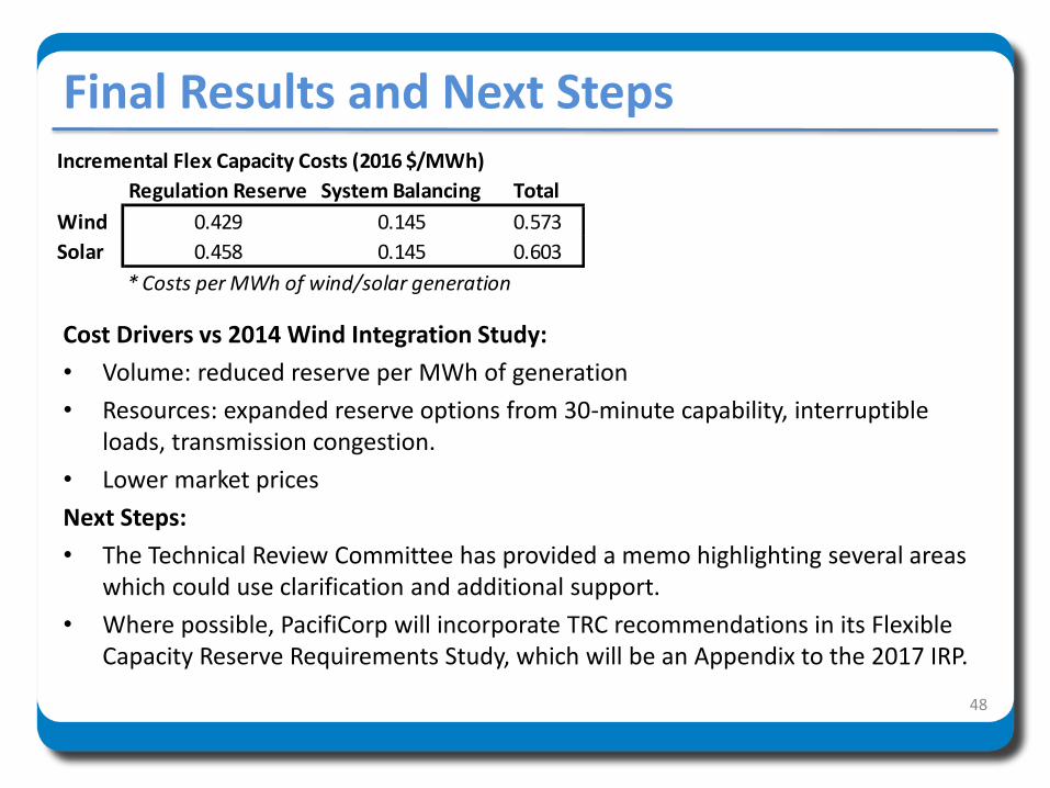
Incremental Flex Capacity Costs (2016 $/MWh)
Regulation Reserve System Balancing Total
Wind 0.429 0.145 0.573
Solar 0.458 0.145 0.603
* Costs per MWh of wind/solar generation
Final Results and Next Steps
Cost Drivers vs 2014 Wind Integration Study:
• Volume: reduced reserve per MWh of generation
• Resources: expanded reserve options from 30-minute capability, interruptible loads, transmission congestion.
• Lower market prices
Next Steps:
• The Technical Review Committee has provided a memo highlighting several areas which could use clarification and additional support.
• Where possible, PacifiCorp will incorporate TRC recommendations in its Flexible Capacity Reserve Requirements Study, which will be an Appendix to the 2017 IRP.
48

2017Integrated Resource Plan
Incremental Solar
Capacity Contribution Results

CF Method with Incremental Resource Additions
• The CF Method assumes that resource output is deliverable to any location where loss of load events occur.
• PacifiCorp has identified several transmission-constrained areas where exports to the rest of the system are limited, or may become limited with incremental resource additions:
– Wyoming Northeast
– Oregon
– Utah South
• In unconstrained areas, the capacity contribution of wind and solar resources remains equal to the LOLP-weighted average of assumed resource capacity factors.
• In a constrained area, capacity contribution has two parts:
– Capacity contribution for events within the constrained area is unchanged.
– Capacity contribution for events outside the constrained area is set at the lesser of the resource’s capacity factor and the available export capability from the constrained area to the rest of PacifiCorp’s system.
• Available export capability is calculated hourly from the same studies used to identify the loss of load events required to calculate capacity contribution with the CF Method.
• Capacity contribution declines as incremental resources use up the available export capability.
50

Exports
Constrained Areas in the 2017 IRP Topology
51
Cholla
4 Corners
$
Utah South
APS
trans
Brady
Goshen
Montana
Bridger West
Colorado
Palo Verde
$
Yakima 2017 IRPTransmission IRP Topology
(2017 to 2036)
Arizona
Borah
Walla Walla
Mona
$
Utah North
Mid-C
$
Mead (Harry Allen)
$
HermistonWyoming NE
Aeolus
Wyoming SW
Chehalis
$
Load
Generation
Purchase/Sale Markets
Contracts/Exchanges
Owned Transmission on PacifiCorp
West East
Portland / N. Coast
Willamette Valley
/ Central Coast
South-Central OR /
N. California
COB
$
Bethel
NOB
$
Bridger
Midpoint
Hemingway
Craig
trans
BPA NITS
Constrained Areas

Export-Adjusted Capacity FactorUtah South +800MW Tracking Solar, Sample July Day
52
0%
10%
20%
30%
40%
50%
60%
70%
80%
90%
100%1 2 3 4 5 6 7 8 9
10
11
12
13
14
15
16
17
18
19
20
21
22
23
24
Cap
acit
y Fa
cto
r (%
)
HourUtah South Export Capability Unconstrained Utah South

0%
1%
2%
3%
4%
5%
6%
7%
8%
0%
20%
40%
60%
80%
100%1 2 3 4 5 6 7 8 9
10
11
12
13
14
15
16
17
18
19
20
21
22
23
24
Loss
of
Load
Pro
bab
ility
(%
of
An
nu
al T
ota
l)
Cap
acit
y Fa
cto
r (%
)
HourCF Method: Unconstrained CF Method: Utah South +800MWUnconstrained Utah SouthLoss of Load Probability
Export-Adjusted Capacity ContributionUtah South +800MW Tracking Solar, Sample July Day
53

0%
10%
20%
30%
40%
50%
60%
70%
80%
90%
100%
Cap
acit
y C
on
trib
uti
on
(%
)
Incremental Capacity Added in Constrained Area (MW)
Tracking Solar - Utah South
Tracking Solar - WyomingNE
Wind - Utah South
Wind - WyomingNE
Incremental Capacity Contribution - East
54

0%
10%
20%
30%
40%
50%
60%
70%
80%
90%
100%
Cap
acit
y C
on
trib
uti
on
(%
)
Incremental Capacity Added in Constrained Area (MW)
Wind - Oregon
Tracking Solar - Oregon
Incremental Capacity Contribution - West
55

Capacity Contribution Results
• CF Method results are based on a CY2020 test period. Transmission availability will be affected by both resource additions and removals.
• IRP models are not equipped to dynamically incorporate the effects of transmission limits on capacity contribution. The unconstrained results (above), will continue to be the primary capacity contribution metric.
• In its portfolio evaluation PacifiCorp will assess whether area capacity limits or tiered capacity contributions are needed to ensure adequate system capacity.
Note: The results presented in the Nov. 17th Public Meeting were based on misaligned hourly LOLP data and have been corrected in the table above. 56
Wind Solar PV
West East Average Wind
West,OR
Fixed Tilt
East, UTFixed Tilt
Average Fixed Tilt
West,OR
Single Axis
Tracking
East, UTSingleAxis
Tracking
Average SingleAxis
Tracking
2015 IRP (CF Approximation)
25.4% 14.5% 18.1% 32.2% 34.1% 33.1% 36.7% 39.1% 37.9%
2017 IRP Updated(CF Approximation)
11.8% 15.8% 14.1% 53.9% 37.9% 45.9% 64.8% 59.7% 62.2%

Corrected Hourly LOLP Alignment
57
0.0%
0.2%
0.4%
0.6%
0.8%
1.0%
1.2%
1.4%
1 2 3 4 5 6 7 8 9 101112131415161718192021222324
Loss
of
Load
Pro
bab
ility
Hour
Loss of Load Probability for Average Day in June
Nov. 17th LOLP Corrected LOLP

0.0%
0.2%
0.4%
0.6%
0.8%
1.0%
1.2%
1.4%
1 2 3 4 5 6 7 8 9 101112131415161718192021222324
Loss
of
Load
Pro
bab
ility
Hour
Loss of Load Probability for Average Day in July
Nov. 17th LOLP Corrected LOLP
Corrected Hourly LOLP Alignment
58

2017Integrated Resource Plan
Preliminary Core Case Results

Core Cases: Introduction• The Company has completed initial simulations for Core Cases 1 through 3.
• Cases 4 through 6 will be presented at the February 23-24, 2017 public input meeting.
• Regional Haze compliance assumptions are based on Regional Haze Case RH-5.– Assumptions include emission control equipment (installations and costs), early
retirements, and associated run-rate operating costs.
– Addresses 2015 IRP stakeholder feedback (ODOE) recommending that Core Cases be compared among common Regional Haze assumptions.
• Core Case portfolios give consideration to more diverse resources. – Ensures relevant operating characteristics are not overlooked.
– Enforcing diverse portfolios provides an additional check against using a simplified set of planning assumptions in portfolio development.
60

Core Cases: Summary
61
Resource Class Case 1(OP-1)
Case 2(FR-1)
Case 3(FR-2)
Case 4(RE-1)
Case 5(RE-2)
Case 6(DLC-1)
Flexible Resources
Optimized10% of
Incremental L&R Balance
20% of Incremental L&R Balance
10% -20% of Incremental L&R Balance
10%-20% of Incremental L&R Balance
Optimized
Renewable Resources
Optimized Optimized OptimizedJust-in-Time Physical RPS Compliance
Early Physical RPS
Compliance
Just-in-Time Physical RPS Compliance
Class 1 DSM Resources
Optimized Optimized Optimized Optimized Optimized5% of
Incremental L&R Balance
All Other Resources
Optimized Optimized Optimized Optimized Optimized Optimized
OP=Optimized FR=Flexible Resources RE=Renewables DLC=Direct Load Control
• Base planning assumptions for each case:
– September 2016 official forward price curve.
– CPP Mass Cap B as summarized for use in the Volume III studies.
• Additional market price and GHG policy assumptions will be analyzed in the cost and risk analysis phase of the process.
• Additional Clean Power Plan assumptions will be analyzed as sensitivities as needed.

Core Cases: Descriptions• Case 1: Optimized Portfolio (OP-1)
– Optimal regional haze case selected as Core Case 1. All resources optimized (selected endogenously by System Optimizer), and valued in the Planning and Risk model.
– Consistent with the approach used in prior IRPs
• Case 2: Flexible Resources (FR-1)– A new fast ramp resource is added to Core Case 1 in the first year (2021)– Added capacity is at least 10% of the system L&R need (578 MW).– Fast-ramp resources available for selection include: SCCT Aero (i.e., LM6000);
Intercooled SCCT Aero (i.e., LMS100); IC Reciprocating Engines; pumped storage, compressed air energy storage, and battery storage.
• Case 3: Flexible Resources (FR-2) – A new fast ramp resource is added to Core Case 1 in the first year (2021)– Added capacity is at least 20% of the system L&R need (1,157 MW).– Fast-ramp resources available for selection include: SCCT Aero (i.e., LM6000);
Intercooled SCCT Aero (i.e., LMS100); IC Reciprocating Engines; pumped storage, compressed air energy storage, and battery storage.
62

Core Cases: Descriptions (Cont’d)• Case 4: Renewable Energy (RE-1)
– Endogenous renewables from Core Case 1 (OP-1) are retained. – Additional renewables are added to physically comply with projected Oregon and
Washington RPS requirements.– Additions are made beginning the first year in which there is a projected
compliance shortfall (just-in-time compliance)
• Case 5: Renewable Energy (RE-2)– Endogenous renewables from Core Case 1 (OP-1) are retained. – Additional renewables are added to physically comply with projected Oregon and
Washington RPS requirements.– Additions are made in 2021 (proxy for year-end 2020) to meet requirements
throughout the planning period (early compliance).
• Case 6: Direct Load Control (DR-1)– Additional Direct Load Control (DLC) is added to Core Case 1 (OP-1) in the first year
(2021).– Added DLC capacity is at least 5% of the system L&R need (289 MW)– Renewable resource assumptions as in Case 4 (RE-1).
63

Core Case: System Optimizer PVRR
• System Optimizer (SO) provides a least-cost capacity-based optimization, enforcing emissions limits and providing shadow price measurement.
• Although the final Regional Haze Case selection is based on the Planning and Risk (PaR) measures, SO results provide an additional indicator and support for the subsequent PaRstochastic results.
• For completed Cores Cases 1 to 3, Core Case 1 (Optimized) yields the lowest PVRR cost.
• Case 2 and 3 added flex resources in 2021 totaling 575 MW and 1,161 MW, respectively.64
15.8 15.7 15.7
7.4 8.0 8.8
$0
$5
$10
$15
$20
$25
$30
OP-1 FR-1 FR-2
PV
RR
$ B
illio
n
System Optimizer PVRR System Costs
Variable Cost Fixed Cost
0.6
1.4
$0.0
$0.2
$0.4
$0.6
$0.8
$1.0
$1.2
$1.4
$1.6
OP-1 FR-1 FR-2
PV
RR
$ B
illio
n
System PVRR Change from OP-1

Core Cases: OP-1 and FR-1 Resource Portfolios
• 667 MW of coal is converted to natural gas or retired by 2025, 2,740 MW is retired by 2036.
• 229 MW of renewables added in 2021, rising to 1,671 MW by 2036.
• 216 MW of gas peaking resource is added in 2029, rising to 797 MW by 2036; 913 MW of CCCT capacity is added in 2030.
• FOTs average 1,003 MW through 2025, and 1,810 MW beyond 2025.
• 1,118 MW of incremental DSM by 2025, rising to 2,386 MW by 2036
65
• 667 MW of coal is converted to natural gas or retired by 2025, 2,740 MW is retired by 2036.
• 236 MW of renewables added in 2021, rising to 2,266 MW by 2036.
• 575 MW of gas peaking resource is added in 2021, rising to 774 MW by 2030; 477 MW of CCCT capacity is added in 2033, rising to 865 MW by 2036.
• FOTs average 780 MW through 2025, and 1,692 MW beyond 2025.
• 1,124 MW of incremental DSM by 2025, rising to 2,451 MW by 2036
(4) (3) (2) (1)
- 1 2 3 4 5 6 7 8 9
20
17
20
18
20
19
20
20
20
21
20
22
20
23
20
24
20
25
20
26
20
27
20
28
20
29
20
30
20
31
20
32
20
33
20
34
20
35
20
36
GW
Cumulative Nameplate Capacity (OP-1)
DSM FOTs Gas
Renewable Gas Conversion Other
Early Retirement End of Life Retirement
(4) (3) (2) (1)
- 1 2 3 4 5 6 7 8 9
20
17
20
18
20
19
20
20
20
21
20
22
20
23
20
24
20
25
20
26
20
27
20
28
20
29
20
30
20
31
20
32
20
33
20
34
20
35
20
36
GW
Cumulative Nameplate Capacity (FR-1)
DSM FOTs Gas
Renewable Gas Conversion Other
Early Retirement End of Life Retirement

Core Cases: FR-2 Resource Portfolio
• 667 MW of coal is converted to natural gas or retired by 2025, 2,740 MW is retired by 2036.
• 238 MW of renewables added in 2021, rising to 2,377 MW by 2036.
• 1,161 MW of gas peaking resource is added in 2021, rising to 1,361 MW by 2033; 477 MW of CCCT capacity is added in 2033.
• FOTs average 520 MW through 2025, and 1,446 MW beyond 2025.
• 1,076 MW of incremental DSM by 2025, rising to 2,254 MW by 2036
66
(4) (3) (2) (1)
- 1 2 3 4 5 6 7 8 9
10
20
17
20
18
20
19
20
20
20
21
20
22
20
23
20
24
20
25
20
26
20
27
20
28
20
29
20
30
20
31
20
32
20
33
20
34
20
35
20
36
GW
Cumulative Nameplate Capacity (FR-2)
DSM FOTs GasRenewable Gas Conversion OtherEarly Retirement End of Life Retirement

$23.6
$23.8
$24.0
$24.2
$24.4
$24.6
$24.8
$25.0
$23.2 $23.4 $23.6 $23.8 $24.0 $24.2 $24.4 $24.6 $24.8
Up
per
Ta
il M
ean
PV
RR
($ b
illi
on
)
Stochastic Mean PVRR($ billion)
Medium Gas, Mass Cap B
OP-1 FR-1 FR-2
$22.8
$23.0
$23.2
$23.4
$23.6
$23.8
$24.0
$24.2
$24.4
$22.6 $22.8 $23.0 $23.2 $23.4 $23.6 $23.8 $24.0 $24.2
Up
per
Ta
il M
ean
PV
RR
($ b
illi
on
)
Stochastic Mean PVRR($ billion)
Low Gas, Mass Cap B
OP-1 FR-1 FR-2
$26.4
$26.6
$26.8
$27.0
$27.2
$27.4
$27.6
$27.8
$28.0
$25.8 $26.0 $26.2 $26.4 $26.6 $26.8 $27.0 $27.2 $27.4
Up
per
Ta
il M
ean
PV
RR
($ b
illi
on
)
Stochastic Mean PVRR($ billion)
High Gas, Mass Cap B
OP-1 FR-1 FR-2
Core Cases: PaR Scatter Plots - Mass Cap B with Fixed Cost
• With fixed costs included in the upper tail mean, which does not change among stochastic iterations, cost and risk are highly correlated.
• OP-1 is least cost, least risk under each price scenario.
• FR-2 produces the highest cost and risk under each price scenario. 67

$23.6
$23.8
$24.0
$24.2
$24.4
$24.6
$24.8
$25.0
$23.2 $23.4 $23.6 $23.8 $24.0 $24.2 $24.4 $24.6 $24.8
Up
per
Ta
il M
ean
PV
RR
($ b
illi
on
)
Stoch
astic Mean PVRR($ billion)
Medium Gas, Mass Cap A
OP-1 FR-1 FR-2
$23.0
$23.2
$23.4
$23.6
$23.8
$24.0
$24.2
$24.4
$22.6 $22.8 $23.0 $23.2 $23.4 $23.6 $23.8 $24.0 $24.2
Up
per
Ta
il M
ean
PV
RR
($ b
illi
on
)
Stochastic Mean PVRR($ billion)
Low Gas, Mass Cap A
OP-1 FR-1 FR-2
$26.4
$26.6
$26.8
$27.0
$27.2
$27.4
$27.6
$27.8
$25.8 $26.0 $26.2 $26.4 $26.6 $26.8 $27.0 $27.2 $27.4
Up
per
Ta
il M
ean
PV
RR
($ b
illi
on
)
Stochastic Mean PVRR($ billion)
High Gas, Mass Cap A
OP-1 FR-1 FR-2
Core Cases: PaR Scatter Plots - Mass Cap A with Fixed Cost
• With fixed costs included in the upper tail mean, which does not change among stochastic iterations, cost and risk are highly correlated.
• OP-1 is least cost, least risk under each price scenario.
• FR-2 produces the highest cost and risk under each price scenario. 68

$16.0
$16.2
$16.4
$16.6
$23.2 $23.4 $23.6 $23.8 $24.0 $24.2 $24.4 $24.6 $24.8Up
per
Ta
il M
ean
PV
RR
Les
s F
ixed
Co
sts
($ b
illi
on
)
Stochastic Mean PVRR($ billion)
Medium Gas, Mass Cap B
OP-1 FR-1 FR-2
$15.2
$15.4
$15.6
$15.8
$22.6 $22.8 $23.0 $23.2 $23.4 $23.6 $23.8 $24.0 $24.2Up
per
Ta
il M
ean
PV
RR
Les
s F
ixed
Co
sts
($ b
illi
on
)
Stochastic Mean PVRR($ billion)
Low Gas, Mass Cap B
OP-1 FR-1 FR-2
$18.8
$19.0
$19.2
$25.8 $26.0 $26.2 $26.4 $26.6 $26.8 $27.0 $27.2 $27.4Up
per
Ta
il M
ean
PV
RR
Les
s F
ixed
Co
sts
($ b
illi
on
)
Stochastic Mean PVRR($ billion)
High Gas, Mass Cap B
OP-1 FR-1 FR-2
Core Cases: PaR Scatter Plots - Mass Cap B, no Fixed Cost
• When fixed costs are removed from the upper tail mean, variable cost risk among portfolios is more apparent.
• OP-1 is least cost and FR-2 is highest cost under each price scenario.
• FR-1 and FR-2 exhibit reduced upper tail variable cost risk relative to OP-1, but the magnitude in risk reduction is much lower than expected total system costs.
69
$16.0
$16.2
$16.4
$16.6
$23.2 $23.4 $23.6 $23.8 $24.0 $24.2 $24.4 $24.6 $24.8Up
per
Ta
il M
ean
PV
RR
Les
s F
ixed
Co
sts
($ b
illi
on
)
Stochastic Mean PVRR($ billion)
Medium Gas, Mass Cap A
OP-1 FR-1 FR-2
$15.4
$15.6
$15.8
$22.6 $22.8 $23.0 $23.2 $23.4 $23.6 $23.8 $24.0 $24.2Up
per
Ta
il M
ean
PV
RR
Les
s F
ixed
Co
sts
($ b
illi
on
)
Stochastic Mean PVRR($ billion)
Low Gas, Mass Cap A
OP-1 FR-1 FR-2
$18.8
$19.0
$19.2
$25.8 $26.0 $26.2 $26.4 $26.6 $26.8 $27.0 $27.2 $27.4Up
per T
ail
Mea
n P
VR
R L
ess
Fix
ed C
ost
s
($ b
illi
on
)
Stochastic Mean PVRR($ billion)
High Gas, Mass Cap A
OP-1 FR-1 FR-2
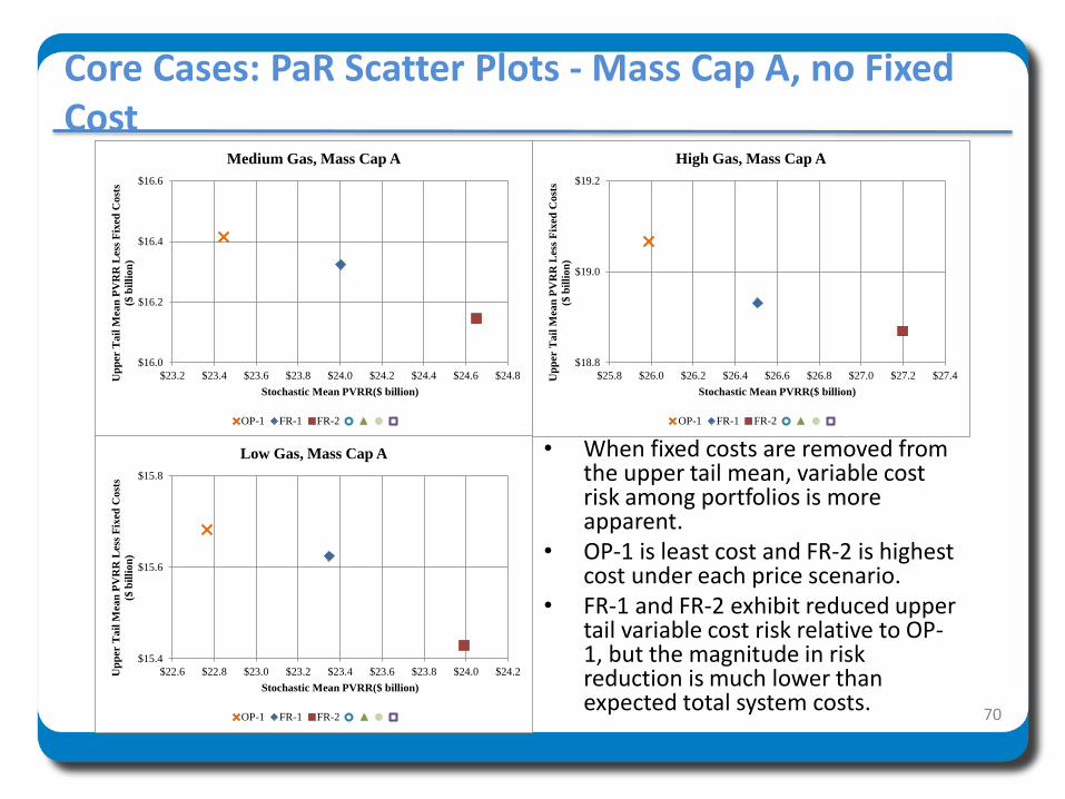
Core Cases: PaR Scatter Plots - Mass Cap A, no Fixed Cost
• When fixed costs are removed from the upper tail mean, variable cost risk among portfolios is more apparent.
• OP-1 is least cost and FR-2 is highest cost under each price scenario.
• FR-1 and FR-2 exhibit reduced upper tail variable cost risk relative to OP-1, but the magnitude in risk reduction is much lower than expected total system costs.
70

Core Cases: Risk-Adjusted PVRR Relative to the Lowest Cost Case
71
• OP-1 produces the lowest risk-adjusted PVRR relative to FR-1 and FR-2 in each price scenario.
• The relative difference between each of the three cases is similar among each price scenario.
$0 $500 $1,000 $1,500
FR-2
FR-1
OP-1
FR-2
FR-1
OP-1
FR-2
FR-1
OP-1
Low
Gas
Med
ium
Gas
Hig
h G
as
$ million
Mass Cap B
$0 $500 $1,000 $1,500
FR-2
FR-1
OP-1
FR-2
FR-1
OP-1
FR-2
FR-1
OP-1
Low
Gas
Med
ium
Gas
Hig
h G
as
$ million
Mass Cap A
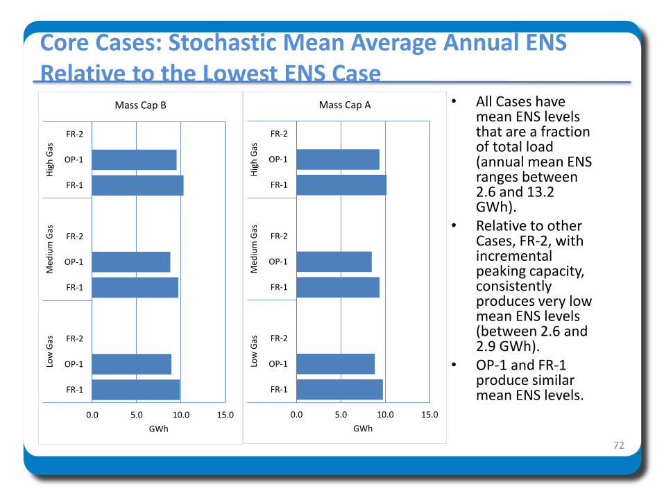
Core Cases: Stochastic Mean Average Annual ENS Relative to the Lowest ENS Case
72
• All Cases have mean ENS levels that are a fraction of total load (annual mean ENS ranges between 2.6 and 13.2 GWh).
• Relative to other Cases, FR-2, with incremental peaking capacity, consistently produces very low mean ENS levels (between 2.6 and 2.9 GWh).
• OP-1 and FR-1 produce similar mean ENS levels.
0.0 5.0 10.0 15.0
FR-1
OP-1
FR-2
FR-1
OP-1
FR-2
FR-1
OP-1
FR-2
Low
Gas
Med
ium
Gas
Hig
h G
as
GWh
Mass Cap B
0.0 5.0 10.0 15.0
FR-1
OP-1
FR-2
FR-1
OP-1
FR-2
FR-1
OP-1
FR-2
Low
Gas
Med
ium
Gas
Hig
h G
as
GWh
Mass Cap A
73
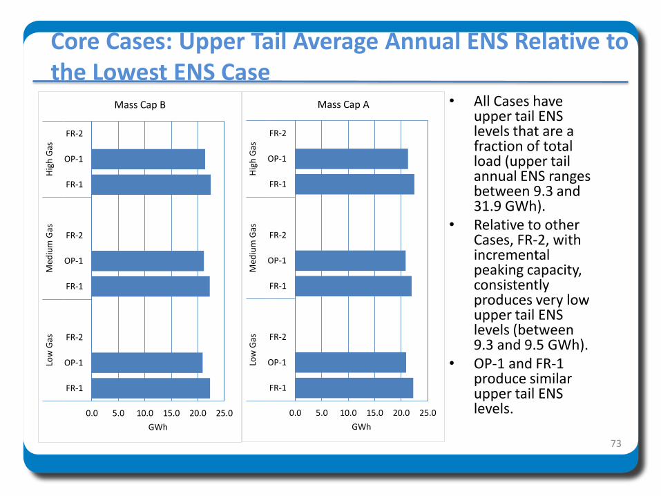
• All Cases have upper tail ENS levels that are a fraction of total load (upper tail annual ENS ranges between 9.3 and 31.9 GWh).
• Relative to other Cases, FR-2, with incremental peaking capacity, consistently produces very low upper tail ENS levels (between 9.3 and 9.5 GWh).
• OP-1 and FR-1 produce similar upper tail ENS levels.
Core Cases: Upper Tail Average Annual ENS Relative to the Lowest ENS Case
0.0 5.0 10.0 15.0 20.0 25.0
FR-1
OP-1
FR-2
FR-1
OP-1
FR-2
FR-1
OP-1
FR-2
Low
Gas
Med
ium
Gas
Hig
h G
as
GWh
Mass Cap B
0.0 5.0 10.0 15.0 20.0 25.0
FR-1
OP-1
FR-2
FR-1
OP-1
FR-2
FR-1
OP-1
FR-2
Low
Gas
Med
ium
Gas
Hig
h G
as
GWh
Mass Cap A

74
• Case FR-1, with flex resource, consistently yields the lowest emissions among all Core Cases, and reported highest renewables added.
• Case OP-1 yields high emissions relative to other cases among the scenarios.
• FR-2 reported next lowest emissions, and was second in renewables added.
Core Cases: Total CO2 Emissions Relative to the Lowest Emission Case
0 2,000 4,000 6,000 8,000 10,000
FR-2
OP-1
FR-1
OP-1
FR-2
FR-1
OP-1
FR-2
FR-1
Low
Gas
Med
ium
Gas
Hig
h G
as
Thousand Tons
Mass Cap B
0 2,000 4,000 6,000 8,000 10,000
OP-1
FR-2
FR-1
OP-1
FR-2
FR-1
OP-1
FR-2
FR-1
Low
Gas
Med
ium
Gas
Hig
h G
as
Thousand Tons
Mass Cap A

Next Steps• Additional Core Cases (RE-1, RE-2, DLC-1) will be completed
and presented at the February public input meeting.
• Additional Sensitivity Cases will be completed and presented at the February public input meeting.
• Upon completion of the additional Core Cases and applicable Sensitivity Cases, the Company will select its preferred portfolio and accompanying action plan (February public input meeting).
75

2017Integrated Resource Plan
Preliminary Sensitivity Results

Sensitivity Cases• Preliminary Sensitivity Case results are benchmarked against Core Case 1
(OP-1), which reflects Regional Haze compliance from Case RH-5.
• Sensitivity cases may be used, as appropriate, to aid the selection of a preferred portfolio, inform the action plan, and inform acquisition path analysis.
• Preliminary list of sensitivities completed to-date:
– CO2 Price, no CPP
– CPP with set-asides but no allocation to PacifiCorp (Mass Cap C)
– CPP with no set-aside program, with new source complement (Mass Cap D)
– Constrained Market (limited FOTs)
– Load Growth (Low / High /1 in 20)
– Private Generation (Low / High)
77

Sensitivity Cases (Continued)• The following Sensitivities will be presented at the February public input
meeting.
– Energy Gateway Transmission• Windstar to Bridger – Segment D
• Gateway South - Segment F
• Windstar to Bridger to Populus and Gateway South
– East/West Split
– Energy Storage
– Wind and Solar Cost (New)
– Regional Haze Case (RH-6), as needed
– Business Plan (as approved 9/15/16; UT Commission Order Docket No. 15-035-04)
– Others
78
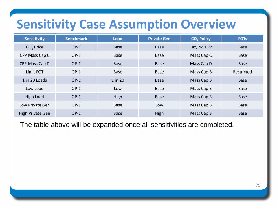
Sensitivity Case Assumption Overview
79
Sensitivity Benchmark Load Private Gen CO2 Policy FOTs
CO2 Price OP-1 Base Base Tax, No CPP Base
CPP Mass Cap C OP-1 Base Base Mass Cap C Base
CPP Mass Cap D OP-1 Base Base Mass Cap D Base
Limit FOT OP-1 Base Base Mass Cap B Restricted
1 in 20 Loads OP-1 1 in 20 Base Mass Cap B Base
Low Load OP-1 Low Base Mass Cap B Base
High Load OP-1 High Base Mass Cap B Base
Low Private Gen OP-1 Base Low Mass Cap B Base
High Private Gen OP-1 Base High Mass Cap B Base
The table above will be expanded once all sensitivities are completed.

Sensitivity: CO2 Price (CO2-1)
• More renewable resources are added, particularly in the out years when the CO2 price increases above $25/ton—less natural gas is added to the system.
• CO2 price included in PaR studies for economic dispatch, but removed for comparison purposes.
• The value of additional renewable resources increases with higher gas prices.
80
$ million
SO PaR Stochastic Mean
Mass B
Mass A
MassA
Mass A
Mass B
Mass B
Mass B
Med Gas
Low Gas
Med Gas
High Gas
LowGas
MedGas
High Gas
PVRR(d) Incr./(Dec.) from OP-1
$928 $1,108 $830 ($353) $1,028 $862 ($368)
(1,500)
(1,000)
(500)
-
500
1,000
1,500
2,000
2,500
3,000
3,500
MW
Increase/(Decrease) in Cumulative Capacity
DSM FOTs Gas
Renewable Gas Conversion Other
Early Retirement End of Life Retirement
$0
$5
$10
$15
$20
$25
$30
$35
$40
20
17
20
18
20
19
20
20
20
21
20
22
20
23
20
24
20
25
20
26
20
27
20
28
20
29
20
30
20
31
20
32
20
33
20
34
20
35
20
36
$/
Ton
Nominal CO2 Price

Sensitivity: CPP Mass Cap C (CPP-C)
• Mass Cap C assumes PacifiCorp does not receive any allocation of set-asides, but the cap only applies to existing resources (new source complement).
• Renewables increase by 71 MW in 2021, but 135 MW fewer renewables added by 2036.
• Timing of natural gas resources is accelerated by one year, but reduced by 99 MW by 2036—combined cycles replace gas-peaking resources.
• High natural gas prices put upward pressure on the mass cap (higher coal dispatch).
81
$ million
SO PaR Stochastic Mean
Mass B
Mass A
MassA
Mass A
Mass B
Mass B
Mass B
Med Gas
Low Gas
Med Gas
High Gas
LowGas
MedGas
High Gas
PVRR(d) Incr./(Dec.) from OP-1
$91 $47 $74 $471 $50 $69 $286
(600)
(400)
(200)
-
200
400
600
800
MW
Increase/(Decrease) in Cumulative Capacity
DSM FOTs Gas
Renewable Gas Conversion Other
Early Retirement End of Life Retirement
20.022.525.027.530.032.535.037.540.042.545.0
20
17
20
18
20
19
20
20
20
21
20
22
20
23
20
24
20
25
20
26
20
27
20
28
20
29
20
30
20
31
20
32
20
33
20
34
20
35
20
36
Mill
ion
To
ns
Mass Cap
Mass Cap B Mass Cap C
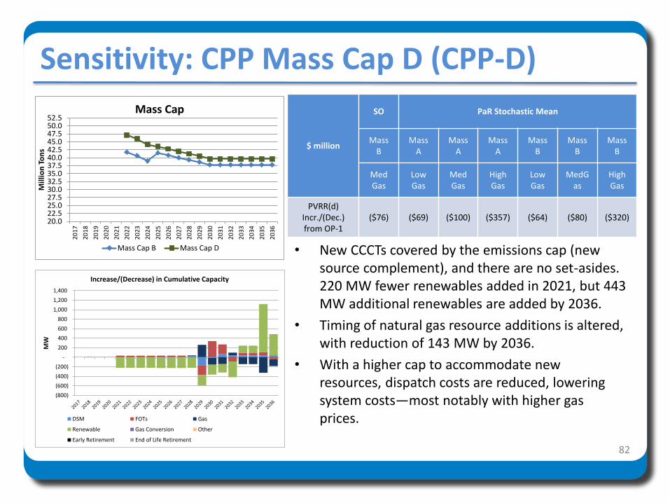
Sensitivity: CPP Mass Cap D (CPP-D)
• New CCCTs covered by the emissions cap (new source complement), and there are no set-asides. 220 MW fewer renewables added in 2021, but 443 MW additional renewables are added by 2036.
• Timing of natural gas resource additions is altered, with reduction of 143 MW by 2036.
• With a higher cap to accommodate new resources, dispatch costs are reduced, lowering system costs—most notably with higher gas prices.
82
$ million
SO PaR Stochastic Mean
Mass B
Mass A
MassA
Mass A
Mass B
Mass B
Mass B
Med Gas
Low Gas
Med Gas
High Gas
LowGas
MedGas
High Gas
PVRR(d) Incr./(Dec.) from OP-1
($76) ($69) ($100) ($357) ($64) ($80) ($320)20.022.525.027.530.032.535.037.540.042.545.047.550.052.5
20
17
20
18
20
19
20
20
20
21
20
22
20
23
20
24
20
25
20
26
20
27
20
28
20
29
20
30
20
31
20
32
20
33
20
34
20
35
20
36
Mill
ion
To
ns
Mass Cap
Mass Cap B Mass Cap D
(800)
(600)
(400)
(200)
-
200
400
600
800
1,000
1,200
1,400
MW
Increase/(Decrease) in Cumulative Capacity
DSM FOTs Gas
Renewable Gas Conversion Other
Early Retirement End of Life Retirement
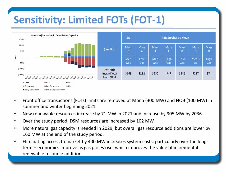
Sensitivity: Limited FOTs (FOT-1)
83
• Front office transactions (FOTs) limits are removed at Mona (300 MW) and NOB (100 MW) in summer and winter beginning 2021.
• New renewable resources increase by 71 MW in 2021 and increase by 905 MW by 2036.
• Over the study period, DSM resources are increased by 102 MW.
• More natural gas capacity is needed in 2029, but overall gas resource additions are lower by 160 MW at the end of the study period.
• Eliminating access to market by 400 MW increases system costs, particularly over the long-term – economics improve as gas prices rise, which improves the value of incremental renewable resource additions.
$ million
SO PaR Stochastic Mean
Mass B
Mass A
MassA
Mass A
Mass B
Mass B
Mass B
Med Gas
Low Gas
Med Gas
High Gas
LowGas
MedGas
High Gas
PVRR(d) Incr./(Dec.) from OP-1
$169 $282 $232 $47 $286 $237 $74 (1,500)
(1,000)
(500)
-
500
1,000
1,500
MW
Increase/(Decrease) in Cumulative Capacity
DSM FOTs Gas
Renewable Gas Conversion Other
Early Retirement End of Life Retirement

Sensitivity: 1 in 20 Load Growth (LD-1)
• 1-in-20 year extreme weather scenario in summer (July) for each state
• Higher peak loads added more FOTs, renewables (+600 MW), DSM (+96 MW), and natural gas (+79 MW) by end of study period
• PVRR(d) costs are higher due to requirements to meet additional peak load.
84
$ million
SOPaR Stochastic
Mean
Mass B Mass B
Med Gas Med Gas
PVRR(d) Incr./(Dec.) from OP-1 $187 $266
(400)
(200)
-
200
400
600
800
1,000
1,200
MW
Increase/(Decrease) in Cumulative Capacity
DSM FOTs Gas
Renewable Gas Conversion Other
Early Retirement End of Life Retirement
9,000
10,000
11,000
12,000
13,000
20
17
20
18
20
19
20
20
20
21
20
22
20
23
20
24
20
25
20
26
20
27
20
28
20
29
20
30
20
31
20
32
20
33
20
34
20
35
20
36
MW
Coincident System Peak Load
Base 1 in 20

Sensitivity: Low Load (LD-2)
• FOTs are reduced by an average of 294 MW through 2029, and increase by an average of 109 MW thereafter with reduced gas and renewable resources.
• Renewable resources are reduced by 687 MW by the end of the study period.
• Natural gas capacity is down by 597 MW by the end of the study period.
• Reduced loads lower system costs significantly.
Lower 85
$ million
SOPaR
StochasticMean
Mass B Mass B
Med Gas Med Gas
PVRR(d) Incr./(Dec.) from OP-1
($1,610) ($1,771)
(1,400)
(1,200)
(1,000)
(800)
(600)
(400)
(200)
-
200
400
MW
Increase/(Decrease) in Cumulative Capacity
DSM FOTs Gas
Renewable Gas Conversion Other
Early Retirement End of Life Retirement
9,000
9,500
10,000
10,500
11,000
11,500
12,000
12,500
13,000
13,500
20
17
20
18
20
19
20
20
20
21
20
22
20
23
20
24
20
25
20
26
20
27
20
28
20
29
20
30
20
31
20
32
20
33
20
34
20
35
20
36
MW
Coincident System Peak (Before DSM)
Base Low Load
55,000
57,000
59,000
61,000
63,000
65,000
67,000
69,000
71,000
73,000
20
17
20
18
20
19
20
20
20
21
20
22
20
23
20
24
20
25
20
26
20
27
20
28
20
29
20
30
20
31
20
32
20
33
20
34
20
35
20
36
GW
h
System Energy Load (Before DSM)
Base Low Load

Sensitivity: High Load (LD-3)
Lower 86
$ million
SOPaR
StochasticMean
Mass B Mass B
Med Gas Med Gas
PVRR(d) Incr./(Dec.) from OP-1
$1,641 $1,799
• FOTs increase by an average of 299 MW through 2028.
• Renewable resources increase by 71 MW in 2021, rising to 360 MW by the end of the study period.
• An additional 200 MW of natural gas capacity shows up in 2028, with 533 MW of additional gas fired capacity by 2036.
• DSM increases by 116 MW by the end of the study period.
• Higher loads increase system costs significantly.
9,000
9,500
10,000
10,500
11,000
11,500
12,000
12,500
13,000
13,500
20
17
20
18
20
19
20
20
20
21
20
22
20
23
20
24
20
25
20
26
20
27
20
28
20
29
20
30
20
31
20
32
20
33
20
34
20
35
20
36
MW
Coincident System Peak (Before DSM)
Base High Load
55,000
60,000
65,000
70,000
75,000
80,000
20
17
20
18
20
19
20
20
20
21
20
22
20
23
20
24
20
25
20
26
20
27
20
28
20
29
20
30
20
31
20
32
20
33
20
34
20
35
20
36
GW
h
System Energy Load (Before DSM)
Base High Load
(200)
-
200
400
600
800
1,000
1,200
1,400
1,600
MW
Increase/(Decrease) in Cumulative Capacity
DSM FOTs Gas
Renewable Gas Conversion Other
Early Retirement End of Life Retirement

Sensitivity: Low Private Gen (PG-1)
• Minor impacts on the portfolio through 2028.
• Over the long-term, there is more renewable capacity (883 MW) and less gas capacity (143 MW).
• Increased net load increases system costs.
Lower 87
$ million
SOPaR
StochasticMean
Mass B Mass B
Med Gas Med Gas
PVRR(d) Incr./(Dec.) from OP-1
$127 $168 9,000
9,500
10,000
10,500
11,000
11,500
12,000
12,500
13,000
13,500
2017 2019 2021 2023 2025 2027 2029 2031 2033 2035 2037
MW
Coincident System Peak (Before DSM)
Base Low PG
55,000
57,000
59,000
61,000
63,000
65,000
67,000
69,000
71,000
73,000
75,000
20
17
20
18
20
19
20
20
20
21
20
22
20
23
20
24
20
25
20
26
20
27
20
28
20
29
20
30
20
31
20
32
20
33
20
34
20
35
20
36
GW
h
System Energy Load (Before DSM)
Base Low PG
(600)
(400)
(200)
-
200
400
600
800
1,000
1,200
MW
Increase/(Decrease) in Cumulative Capacity
DSM FOTs Gas
Renewable Gas Conversion Other
Early Retirement End of Life Retirement

Sensitivity: High Private Gen (PG-2)
• Minor impacts on the portfolio through 2028.
• Over the long-term, there is an more renewable capacity (1,108 MW) and less gas capacity (597 MW).
• Decreased net load decreases system costs.
Lower 88
$ million
SOPaR
StochasticMean
Mass B Mass B
Med Gas Med Gas
PVRR(d) Incr./(Dec.) from OP-1
($278) ($273) 9,000
9,500
10,000
10,500
11,000
11,500
12,000
12,500
13,000
13,500
20
17
20
18
20
19
20
20
20
21
20
22
20
23
20
24
20
25
20
26
20
27
20
28
20
29
20
30
20
31
20
32
20
33
20
34
20
35
20
36
MW
Coincident System Peak (Before DSM)
Base High PG
55,000
57,000
59,000
61,000
63,000
65,000
67,000
69,000
71,000
73,000
20
17
20
18
20
19
20
20
20
21
20
22
20
23
20
24
20
25
20
26
20
27
20
28
20
29
20
30
20
31
20
32
20
33
20
34
20
35
20
36
GW
h
System Energy Load (Before DSM)
Base High PG
(1,000)
(500)
-
500
1,000
1,500
2,000
MW
Increase/(Decrease) in Cumulative Capacity
DSM FOTs Gas
Renewable Gas Conversion Other
Early Retirement End of Life Retirement

2017Integrated Resource Plan
Next Steps

Next Steps
• Next 2017 IRP Public Input Meeting
– February 23-24, 2017
– Topics:
• Remaining Study Results
• Preferred Portfolio
• Action Plan
90

Additional Information• Meeting presentation and materials:
http://www.pacificorp.com/es/irp.html
• 2017 IRP Stakeholder Feedback Form:
http://www.pacificorp.com/es/irp/irpcomments.html
• Email / distribution list contact information:
• Upcoming Public Input Meeting Dates:
– February 23-24, 2017
91