University of Toronto Winter 2016

Department of Economics

Master of Financial Economics

ECO2505H Macro Policy Analysis and Forecast

Canadian 2016 Federal Budget - Economic Impact

Wladimir Hinz Baralt, 1001800107

Ying Zhu, 998527802

Introduction

On March 22, 2016, Bill Monreau, the Federal Minister of Finance, presented the newly

elected Liberal government’s first budget. As a platform for implementing distinctive election

promises, the budget plan is particularly straightforward about what the new majority’s intentions

are for the next couple years. Justifiably called Growing the Middle Class, the budget proposes

several tax initiatives and other non-tax measures, such as significant investments in infrastructure

and clean technology, as well as the revision of earlier policies that overall signify a profound

regime change. It sends a clear message about what the government’s intention is: to reduce

poverty and fortify the middle class by strengthening the economy.

A detailed review of the plan suggests that the measures are set in a framework that is

sound enough to appeal to those who worry about excessive government spending. Even though

the budget is deficit financed, with a projected total of $29.4 billion (roughly 1.5% of GDP) for

2016-2017, the general consensus suggests that this is a prudent number. Most economists were

expecting a much higher amount, with some suggesting that the government could have gone as

high as $40 billion. It is also relevant to mention that figures ranging from the Governor of the

Bank of Canada, the Canadian Centre for Policy Alternatives and the C.D. Howe Institute, had

recommended that the government propose a modest deficitary budget. The reason behind this is

that the interest level remains at historic lows, so servicing a modest debt is still affordable.

Without such deficit spending, it would not be possible to address the much needed

investments in infrastructure and in social well being, particularly those concerning the middle

class and the first nations peoples.

The 2016 Budget

The main points from the budget plan can be summarized as follows:

Benefits and Tax Credits:

a. The Canada Child Benefit (CCB) is created to replace the Universal Child Care Benefit, starting

July 1, 2016. The plan states that monthly tax free payments will be given to parents and can be

up to $6,400 each year for every child less than 6 years old, and $5,400 each year for those between

6 and 18 years. This measure also conditions the CCB on the households’ income, eliminating it

completely for families above the $190,000 earnings per year bracket. This suggests a more

efficient way to give aid to those who require it the most.

b. The Children’s Arts and Fitness tax credits is set to be eliminated after 2017. Some additional

funds will be made available for teachers for teaching materials.

c. The Education Tax Credit and the Textbook Tax Credit are set to be eliminated after 2017, as they

state that these tax credits do not help the students that are in most need of aid.

d. Changes in the tax brackets and on the tax rates:

- 4% increase in the top federal rate of personal income tax (from 29% to 33%) for taxable

income over $200,000;

- a reduction in the second-lowest federal tax bracket rate from 22% to 20.5%;

- a reduction in the annual Tax-Free Savings Account contribution limit from $10,000 to

$5,500; and

- changes to several tax measures affecting Canadian-controlled private corporations (CCPCs)

and other private corporations.

Student Loans and Grants:

Student Grants are increased by 50% so that they change:

- from $2,000 to $3,000 per year for students from low-income families;

- from $800 to $1,200 per year for students from middle-income families; and

- from $1,200 to $1,800 per year for part-time students.

Student loans repayments are also set to start after the students’ earnings are beyond the

$25,000 threshold.

Employment Insurance (EI):

It can be seen as a complete renovation of the EI system. It includes temporary enhanced

benefits for a number of regions where the unemployment problem is most severe, particularly

regions in North Canada, Newfoundland and Labrador, and those that had been touched by the

low oil and gas prices. More generally, it lowers the amount of hours that claimants require to be

eligible – which vary from region to region -, as well as it lowers the wait time to start receiving

the benefits from 2 weeks to 1, reducing the time without income for those who lose their jobs.

A significant amount of funds will be also spent on improving call centres and to ensure that the

process to apply for EI is made more swiftly.

Regarding premiums paid to employees, they are expected to drop in 2017 from $1.88 for

every $100 they earn to $1.61, but which is still higher than the drop to $1.52 scheduled by the

earlier Conservative government.

Infrastructure Investments:

A high percentage of the deficitary budget comes from infrastructure investment in projects

all over Canada. Most of the infrastructure spending will go to investments in public transit,

followed by investments that will be done for water/waste related structures in First Nations

communities. The distribution for the first year of the infrastructure budget is as follows:

- $3.4 billion for public transit

- $2.2 billion for water/waste structures in First Nations communities

- $1.4 billion for affordable housing

- $518 million for climate change mitigation technologies

- $400 million for early learning and child care

There is also $4 billion set to be spent in other miscellaneous projects. In total, over the

next 10 years, the government is set to spend $120 billion.

Arts Investments:

Approximately $ 1.9 billion is set to be spent on Canada’s national museums and art

centres. There will be also an amount going to the CBC and Radio Canada.

Direct Transfers:

For seniors and veterans, there will be an increase in the Guaranteed Income Supplement

and an increase in the amounts paid to those who have been injured in service, respectively.

First Nations Peoples:

One of the sectors of society that will see an important amount of aid is the First Nations

communities, who expect to see funding of $ 8.4 billion for different projects (including the

water/waste infrastructure investments) over the next 5 years. Additional funds provided will be

destined to improvements in schools offering primary and secondary educations present on the

reserves, and to develop and sustain family and child services.

Considering these major points, there are also many other, though relatively smaller,

measures proposed in the budget. As mentioned before, overall, this accounts for a budget that will

run on a deficit of $29.4 billion for 2016-2017, a deficit that will slowly go down over the next 5

years, but that will still remain over $14 billion in 2020 – 2021, as can be seen in Table 1.

Furthermore, two special caveats can be drawn from the budget. The first one is the

assumed rate of growth for the GDP that has been used for all the periods, which is substantially

lower than the one that has been brought up by numerous economists. The government is assuming

that the economy will only grow 0.4% in nominal terms during the 2016 year, quite shy from the

2.4% that is agreed on by consensus. The second one is the price of oil, which is also set at a lower

level than what it currently is. Both decisions can be interpreted as subtle political strategies, used

by the government to beat “easier” benchmarks and to have the ability to expand spending further

afterwards.

Expected Results from the Measures of the 2016 Federal Budget

From the measures proposed on the budget, we can draw the following expected effects:

Poverty Reduction:

We believe that the changes introduced by the government, should almost surely have an

impact on the levels of poverty in Canada. The federal budget has introduced a new way of

delivering child benefits to those households that are most in need of supplemental aid, using

resources more efficiently by adjusting the distribution of funds to better reflect the economic

conditions of each family. This is also strengthened when such benefits are increased.

On another front, the budget also looks to reduce poverty among seniors by reverting to 65

the age of eligibility for Old Age Security (OAS) and Guaranteed Income Supplement (GIS),

which is similarly strengthened by increasing the GIS transfers.

Unemployment Reduction:

For unemployed Canadians, the budget seeks to improve access and the performance of

Employment Insurance, in particular to precarious workers and recent immigrants. The fiscal

spending will also bring new jobs for the programs and projects that are set to be completed, as

they will require more employees to be done. Given the current unemployment levels, which are

very close to the NAIRU, real wages will probably rise in response to the higher demand of

workers, which will in turn, generate certain inflationary pressures as prices are adjusting in the

economy to account for the new wages.

GDP Expansion

Overall, we expect to see a very strong expansion of the GDP which is driven entirely by

the fiscal stimulus, much more than the moderate levels of growth projected by the government.

Given that the stimulus does not stop after the first year, given that it is not an individual shock,

the GDP growth is expected to continue, still at higher levels than are being projected.

FOCUS Model

To model the effects of the 2016 budget on the Canadian economy, we use the FOCUS

model developed and maintained by the Institute for Policy Analysis at the University of Toronto.

This is quarterly macroeconomic model that consist of a system of 300 equations that are built on

the IS-LM analytical framework and incorporate a Philips curve that takes into account inflation

expectations.

Due to the way the model is set up, we forecast the behaviour of the economy for the 3

calendar years 2016, 2017 and 2018. We do not use the intra year (2016 – 2017, 2017 – 2018 and

2018 – 2019) way the budget is set up. Additionally, we analyze the impact of the measures

contained in the budget with 3 different types of monetary policy responses. The Base Case run of

the model considers a neutral response by the Bank of Canada where the M1 is held fixed at

historical levels. The second run of the model considers a monetary policy that follows the Taylor

Rule and the third run looks at what happens when the historical exchange rate is deemed the target

of monetary policy.

To input the data on the model, we match each rubric of the budget to its corresponding

variable in the model, the total amounts are presented in Table 2. We identify 5 main variables that

get affected by the measures:

GCF: Government Current Expenditures

GIF: Government Gross Capital Formation

REGBEN: Regular Employment Insurance Benefits Paid

TDPYF: Personal Income Taxes

TRGPFN: Other Transfers to Persons, Non Taxable

Base Case Results

A summary of the Base Case projection can be seen in Table 3.

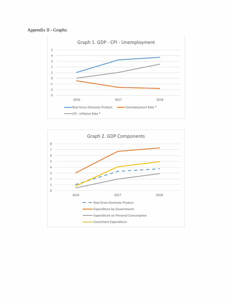
As expected, GCF and GIF contribute strongly to real GDP growth, as can be seen in Graph

2. Both expenditure by governments and investment expenditure see an important positive reaction

motivated by the federal government fiscal stimulus. These two accounts grow much faster than

the real GDP, which is expected as it is the beginning of the stimulus. The complete effect of the

effect on GDP would be projected to be seen much after the forecasting period as more of the

investment expenditures come into effect.

According to the 2016 budget, the bulk of investment expenditure is to happen in the earlier

years, but since these projects will take some time to be finished and to start contributing to

economic growth, we would need consider more time (years) into our forecast to see this effect

completely translate into GDP growth. This is especially true if we take into account that some of

the expenditure by the government is going into health care, which will likewise take some time

to be incorporated into the economy as growth.

Another driver of GDP growth is expenditure on personal consumption. When we look at

the equations that determine this variable in the FOCUS model, it is not surprising to see a positive

effect since two of the variables used to compute personal consumption are the transfers that

government gives to households (TGRPFN) and the personal income taxes that it collects from

them (TDPYF). Since both effects are in play here, and they are both contributing to higher

personal income, the total effect captured in largely positive. We can see this in Table 4 and in

Graph 3.

Transfers to households, the tax cuts and the grants announced in the budget enter into

these variables stated above (including the OAS payments, Employment Insurance and the

Veterans’ aid).

The effects on inflation (CPI) and unemployment (U) are also in line to those expected,

and are also in line to the historical responses to these changes in the economy. In Graph 4, we can

see the effects of the Philips curve at play; inflation starts picking up immediately in response to

the fiscal stimulus, and it continues to rise as the government spending does not cease. Since under

this model there is no strong response from the Bank of Canada to counter these effects, real wages

adjust for the higher level of prices, unemployment begins to fall, and real wages starts to rise.

Interest on the debt (TRGIDF), naturally, rise. This is comprehensible as the budget is

being run on a deficit, though it is important to note the amount by which it changes, over 2016-

2018 it increases 0.9%, 4.5% and 7.9%, respectively. Servicing the debt becomes more expensive

as it increases each year and it reaches $2.7 billion by 2018 (just interest), but considering that at

this point the government will be indebted approximately $80 billion, in relative terms, is still

seems affordable. Yet, as we can see in Graph 5, this also affects the government bond rates

(RDFUs Variables). All of them rise for the period of study, but given that the interest rates are at

a historical low, this rise does not produce important changes to the costs of financing.

We now turn to the revenue side of the budget, where we can identify 3 important variables

of interest: corporate (TDCF), personal (TDPF) and indirect taxes (TIF).

For the corporate taxes, we do not identify any changes in the 2016 budget (most likely it

will be left to the provincial level), which is why we observe such high increase of corporate

profits. Corporate tax collection rises for all years except the first one, when it sees a decline

motivate by the adjustment of prices in the economy. Personal taxes and indirect taxes also see

increases in the model. The first driven by the government expenditure and the raise of personal

income (which is linked to what happened to consumption before, so the analogous analysis

applies here) and the second is driven mainly by government fixed capital investment and current

expenditure, which are the variables that were changed to model the behaviour of the economy

taken directly from the budget.

One last important variable where we see changes is in net imports (M-X). They increase

significantly as the Canadian dollar depreciates relative to the US dollar. This is what is expected

in this base case where the Bank of Canada does not react to control the effects of the fiscal

stimulus, and the exchange rate has to consider the current account and long term capital account

balances as well as the short term flows.

Alternative Cases

For the Alternative Cases, we study two possible monetary policy responses from Bank of

Canada with respect to the new federal budget – ‘Taylor Rules’ (Rule M3) and exchange rate

targeting (Rule M6). Under M3, deviations of inflation from its target rate and deviations of GDP

from its potential are determined first, which are used to set interest rates as the deviations from

long-run equilibrium values. Under M6, exchange rate is fixed and interest rate is found to balance

the payments to the exogenous target change in international reserves. Given the current condition

of the economy, the Bank of Canada is more likely to pursue Rule 3, rather than Rule 6, given the

current oil price. However, if the oil price can rebound and remain stable, Rule 6 is also possible

in order to prevent more capital outflow to U.S. Therefore, both cases are analyzed. By

incorporating these monetary policies into FOCUS model, we get two sets of projections with

noticeable variations on multiple variables. Table 5, shows the summary projections of major

economic factors under two monetary policies, given the new 2016 federal budget.

Government Expenditure

Government expenditure is adjusted with the new 2016 federal budget. Therefore, both

cases should exhibit similar reactions regarding government expenditure. Projection results from

FOCUS confirm that both cases have similar positive shocks on government expenditure sector.

Under M3, government expenditure increases 3.02% in 2016, 6.60% in 2017 and 7.20% in 2018

over the base case. In terms of the case with rule M6, those number are 3.05%, 6.66% and 7.23%

respectively.

Investments

Rule M3 suffers severe kickback effects from the high inflation caused from the new

federal budget. In that case, real GDP can only have positive shocks for first two years with 0.70%

hike of 2016 and 0.78% hike of 2017 respectively. In 2018, real GDP will even decline under new

physical expansionary policy. On the other hand, under M6 rule, real GDP can enjoy positive

shocks for next three years, with 0.99% hike of 2016, 2.38% hike of 2017 and 1.59% hike of 2018.

In general, having physical expansionary policy can stimulate the economy significantly.

However, under rule M3, at the beginning of expansionary policy, it leads to high inflation and

high potential GDP, which results in a high interest rate (that matches the long run equilibrium

values). Based on the Taylor rule, if there is one percent increase in inflation, the central bank

should raise the nominal interest rate by more than one percent to offset the effect. High interest

rate then limits the impact of the fiscal stimulus on Canadian economy. Graph 7 shows the long

term and short term real interest movements for both cases.

If the Bank of Canada wants to follow Taylor rule to make corresponding interest rate

adjustments, the Canadian economy has to bear a much higher interest rate shock in comparison

to the base case. Both short term real interest rate (RMRLF) and long term real interest rate

(RMRL1) reach the peak in 2017 with 48.54% and 56.31% positive shocks over the base case

respectively. In 2018, RMRLF fades from 4.00% to 3.39% and RMRL1 declines from 4.27% to

4.08%. On the other hand, if Bank of Canada would rather maintain the exchange rate, it will still

cause both RMRLF and RMRL1 to increase, but much lower and smoother than that under Taylor

rule. By having exchange rate targeting monetary policy, RMRLF and RMRL1 tend to increase

gradually. RMRLF peak at 3.02% in 2017, with a 12.07% positive shock over the base case.

Moreover, RMRL1 increases from 1.97% of 2016 to 3.77% of 2018, with positive shocks of 8.90%

and 34.11% over the base case.

In theory, by having much a higher real interest rate, personal and national investments can

be severely impacted, leading to a much lower total investment number. FOCUS model also

produces similar projections regarding real investment expenditure.

Under M3, total real investment expenditure decreases 0.14% in 2016, -2.87% in 2017 and

6.03% in 2018 compared with those in base case. This is due to negative reactions all over

Residential Construction (IFHB), Non-Residential Construction (IFNB) and Machinery and

Equipment Investment sectors (IFMB). Based on the calculation methodology used in FOCUS,

those negative shocks can be explained in terms of the negative shock on initial stock and the

difference between internal and external after-tax return. The value of stock of private residential

(KFHB) decreases after adjusting for higher real interest rate, which results in much lower IFHB.

Similarly, stock of machinery and equipment has its value diminished. For IFNB, the value of

stock of non-residential structure declines as well as the difference in internal and external after-

tax return (RRDIF). In this case, both factors reduce the value of IFBN. Therefore, the overall real

investment is much lower than the original level. The quick hike of real interest rate limits the

investment significantly, the negative impact of which overweighs the positive impact from

physical expansionary policy. Therefore, the overall real investment number declines.

Under M6, the similar rational is applied as discussed above. However, real interest rate

hike in this case is much smaller in terms of the scale, and the path is much smoother. The positive

impact from new federal budget still dominant the overall effect. Therefore, all investment sectors

enjoy positive shocks in first two years. In the third year, as real interest rate gets even higher, the

benefit from expansionary policy is unable to cover the decline from high real interest rate, leading

to negative changes.

Consumption

Personal consumption increases after adopting the new federal budget for both monetary

policies. Under the new expansionary government budget, it reduces the income tax rate for middle

income taxpayers, and increases grants in multiple social areas including educations.

Theoretically, those policy changes can improve consumption. Under M3, personal consumption

raises 0.42% in 2016, 1.37 % in 2017, and 1.57% in 2018, over the base case. On the other hand,

by having M6 for the monetary policy, personal consumption raises 0.47% in 2016, 1.79% in 2017,

and 2.33% in 2018 over the bae case. The second case improves consumption more, given it has

more national investments as well. In FOCUS model, consumption is mainly determined by

permanent income per adult (YPPMHR). According to Graph(s) 8, monetary rule M6 allows

individual citizen to accumulate more permanent income, mainly due to a much higher aggregate

national disposable income (YPD).

There are various reasons that why the case with M6 monetary policy has a much higher

disposable income. First, M6 has a better employment data compared with that of that under M3.

Based on Philips Curve, higher inflations will lead to lower unemployment rates. FOCUS model

tries to determine wage rates, employment and the labor force participation rates by matching the

labor supply and the aggregate production. Graph(s) 9 show the summary results of CPI data

(CPI) and unemployment rates (RU) for both cases. Under M3, CPI rates are 1.31% in

2016, 1.35% in 2017 and 1.40% in 2018, and unemployment rates are 6.23% in 2016, 5.94% in

2017 and 5.82% in 2018. Meanwhile, under M6, Under M3, CPI rates are 1.31% in 2016, 1.35%

in 2017 and 1.38% in 2018, and unemployment rates are 6.15% in 2016, 4.96% in 2017 and 5.13%

in 2018. For the case of M3, Interest rate is adjusted more than the change of CPI, and then limits

the effect of the expansionary government policy. Therefore, CPI rates are controlled within the

range of long-run CPI target. However, under M6, it maintains exchange rate, not CPI, which has

less interest rate hike and more CPI growth. Consequently, it has better employment data compared

with that under M3. Furthermore, FOCUS models the labor market as the short term trade-off

between wage inflation and unemployment rates. Therefore, this relationship is unable to hold in

long-run, which explains why the unemployment rate in 2018 is higher than that of 2017 given the

same monetary policy.

Second, as we discussed before in investment part, M3 rule actually discourages

investment activities, restricting the production development. This problem reinforces back to the

labor market, as production is one concern to achieve the employment rate. Therefore, since M6

rule leads to a higher production potential, it results in a relatively higher employment rate.

Third, total labor force and participation rates raise more in the case with monetary policy

M6 compared with that with M3. Under M3 (M6), labor force level increases 11.37 (14.24)

thousand in 2016, 62.17 (94.00) thousand in 2017 and 70.44 (140.36) thousand in 2018. In terms

of the participation rate, it improves 0.04% (0.05%) in 2016, 0.21% (0.32%) in 2017, and 0.23%

(0.47%) in 2018 with M3 (M6) monetary policy. Both results indicate that M6 rule encourages

more people to enter the labor market, allowing more labor supply.

By implementing M6 rule, the society is able to have lower unemployment rates and higher

wages, according to Philips Curve, with a larger labor force size. It is reasonable that the national

disposable income for the M6 case is higher than that for the case with M3. Consequently, given

the higher national disposable income and lower unemployment rate, the permanent income per

adult gets higher. Ultimately, it can encourage more private consumption.

Exports and Imports

For both cases, exports and imports movements for next three years are indicated in

Graph(s) 10. Exports numbers are lower in both cases compared with those in the base case. Under

M3 (M6), exports value decreases 0.12% (0.00%) in 2016, 0.66% (0.06%) in 2017 and1.57%

(0.33%) in 2018, while its imports value increases 0.54% (0.33%) in 2016, 2.25% (1.79%) in 2017

and 3.20% (3.07%) in 2018. Exports and imports numbers are mainly impacted by exchange rate,

which is float under M3 and fixed under M6.

Under M3, DFX is set to be 1, indicating that the exchange rate Canadian dollars per US

(RXUS) is determined within the model by equalizing the balance of the payment. Meanwhile,

capital service receipts (XSCAPV) will be fixed at zero. US three-month Treasury bill rate (USRMTB)

and US corporate bond rate (USRMAA) are exogenous and remain same as the base case. Then,

FOCUS tries to search for the exchange rate that equalizes official settlement balances (BPOS)

with the sum of three balances - current account (BPC), net capital movement in short-run (BPSN)

and new capital movement in long-run (BPLN). As we discussed before, M3 monetary policy

forces central bank to make interest adjusted based on Taylor rule, leading to much higher nominal

and real interest rates compared with those under M6, given the new federal budget. In FOCUS

model, both Canada-US short-rate differentials (RDFUS) and long-rate differentials (RDFUL)

increase significantly. RDFUL has its level increased 0.58% in 2016, 1.71% in 2017 and 1.21% in

2018. Similarly, RDFUS increases for next three years as well. Higher real interest rate relative to

U.S. attracts more capital inflow to Canada in long-run, while in short-run the current account may

have to face the presence of a J curve. Therefore, the value of BPLN surges significantly each year,

which is then offset by decline in BPC and BPSN. This iteration results in a lower RXUS value,

which aligns with the theoretical intuition. Therefore, under M3, Canadian dollar appreciates

against U.S. dollar, in order to balance all trade accounts. For the case with M6 rule, exchange rate

RXUS will be set as target and remain same for all three years. Therefore, RXUS in M3 is lower

than that in M6. In other words, if Bank of Canada decides to use Taylor rule to make

corresponding adjustments to the physical expansionary policy, Canadian dollar will start to

appreciate a lot. Graph(s) 11 show the exchange rate projections for next three years for both cases.

Total real exports (X) and real imports (M) have the most direct impact from CAD

appreciation. The actual regression function for X can be found on page 83 of the FOCUS manual,

while we use the function of real exports calculated as sum of components (XTOTL) to illustrate

the fact. In the case with M3 as the monetary policy, by having a lower RXUS, it increases the

exports of auto and parts (XGAUS), exports of goods (XGO), and also exports of services (XS).

The exports of petro and natural gas are traded in US dollar originally, which are influenced by

the exchange rate. As a result, Canadian real exports are lower than before, and the effect is further

amplified as CAD keeps appreciating. Similarly, for real imports (M) (page 85), the sum of imports

components (MTOTL) is used to show how each explanatory factor is influenced. Imports of auto

and parts (MGAUS) (page 77) are positive correlated to the XGAUS. Since XGAUS gets smaller

due to the lower RXUS, MGAUS declines as well. As RXUS decreases, the deflator of imports of

other merchandise (PMGO) (page 76) is smaller, which leads to a much higher number of imports

of goods (MGO) (page 73) due to the exponential effect. Imports of service (MS) is primarily

driven by the domestic GDP. Since GPD increases, MS rises accordingly. All of three factors tend

to increase, resulting a higher value of M. Under M6, it also has its interest rate increases each

year, but in a much smoother path that used to maintain the exchange rate. In this case, since RXUS

remain same as the base case level, the extra impact from RXUS will not be considered in the

exports and imports analysis. The exchange rate difference between two cases is the main reason

behind their exports and imports movements. Furthermore,

Overall, by having higher interest rates, M3 rule forces Canadian dollar to appreciate,

resulting in a lower value of RXUS. Consequently, this case outputs relatively higher imports

values and lower exports values, in comparison to the case under M6. In the end, net exports for

the case under M6 increase more than the one under M3, allowing to have more contribution to

the GDP growth.

After Event Government Balance

In both cases, we would expect to see a huge government deficit after implementing the

new federal budget. However, under M3, the government has to face a much higher amount of

outstanding deficit, compared with that of M6. Under M3 (M6), the consolidated government

balance will decrease 10,929 Mill (8,911Mill) in 2016, 20,605 Mill (6,823 Mill) in 2017 and 30266

Mill ( 8738 Mill) in 2018. The majority of the deficit comes from the federal government, which

makes intuitive sense in this case as they are the driver for the current physical expansionary

policy.

The cause of much higher government deficit in the case with M3 is the overall effect from

each component of GDP. The main purpose of establishing the new federal budget is trying to

stimulus the economy. However, by having Taylor rule as the monetary policy, the central bank

has to make even more severe contractionary monetary policy changes to minimize the effect

caused by inflation. Therefore, the overall expansionary effect on the economy is also minimized,

leading to small or even negative GDP changes. The government is unable to recollect capital back

though taxes, while they still have to keep their spending. Therefore, the outstanding balance

deficit for the case with M3 rule is much higher.

Conclusion

The new 2016 government budget is extremely important in the current Canadian

economy. Given the current low prices in commodity market, Canadian economy has been

suffering from low or negative for a long period. Bank of Canada has decided to maintain the

overnight rate twice to wait for the new physical expansionary policy and then make possible

monetary policy adjustment afterwards.

In this paper, it discusses two possible reactions from Bank of Canada – Taylor rule and

exchange rate targeting. However, we do not expect to see these two potential movements from

Bank of Canada. For Taylor rule, we believe it is very unlikely that Bank of Canada will use it.

These monetary adjustments will diminish the efforts that the government made to accelerate the

growth of economy, which even worse, will slow down the economy further. For exchange rate

targeting, we do not expect to see this policy from Bank of Canada as well, given the current low

and volatile price. Current oil price is still lower than the average production cost for most

Canadian producers. Many producers relay one the exchange rate to maintain relative lower cost

(cost in CAD) but higher revenue (sales in USD). Bank of Canada is unable to make any exchange

rate decision until the commodity market stabilizes.

References

2016 Federal Budget. (2016, March 22). Retrieved April 14, 2016, from

http://www.budget.gc.ca/

Dungan, P. (2000) The Effect of Workers' Compensation and Other Payroll Taxes on the Macro

Economies of Canada and Ontario, in New Perspectives on Workers' Compensation

Policy (edited by Gunderson, Morley and Hyatt, Douglas), University of Toronto Press, 118–161

Dungan, P. (2011). “Quarterly Forecasting and User Simulation Model of the Canadian

Economy.” Institute for Policy Analysis - Rotman School of Management, University of

Toronto.

Dungan, P., & Wilson, T. (1985). Altering the Fiscal-Monetary Policy Mix: Credible Policies to

Reduce the Federal Deficit. Canadian Tax Journal. March-April

Dungan, P., Mintz, J., Poschmann F., & Wilson, T. (2008) Growth-Oriented Sales Tax Reform for

Ontario, C.D.Howe Institute Commentary No. 273

Romer, D. (2012). Advanced macroeconomics. New York: McGraw-Hill/Irwin.

Taylor, J.B. (1999) “The Robustness and Efficiency of Monetary Policy Rules as Guidelines for

Interest Rate Setting by the European Central Bank.” Journal of Monetary Economics 43(3): 655–

79.

Appendix I - Tables:

Table 1. Federal Budget Fiscal Projections (in billions of $)

2015 - 2016 2016 - 2017 2017 - 2018 2018 - 2019 2019 - 2020 2020 - 2021

Revenues 291.2 287.7 302 315.3 329.3 344.4

Expenses 296.6 317.1 331 338 347 358.6

Program Expenses 270.9 291.4 304.6 308.7 314.2 323.2

Public Debt Charges 25.7 25.7 26.4 29.4 32.8 35.5

Federal Debt 619.3 648.7 677.7 700.5 718.2 732.5

Debt-to-GDP Ratio 31.2 32.5 32.4 32.1 31.6 30.9

Deficit 5.4 29.4 29 22.7 17.7 14.2

Source: 2016 Budget

Table 2. Input for the Model

Variable 2016 2017 2018

Q1 Q2 Q3 Q4 Q1 Q2 Q3 Q4 Q1 Q2 Q3 Q4

GCF 72 72 17,928 17,840 17,715 17,628 22,349 22,241 22,058 21,967 21,863 21,774

GIF -151 -150 2,400 2,388 2,378 2,364 3,506 3,489 3,469 3,452 3,432 3,416

REGBEN 0 0 1,018 1,018 1,018 1,018 1,449 1,449 1,449 1,449 1,449 1,449

TDPYF 370 370 1,084 1,084 1,084 1,084 622 622 622 622 622 622

TRGPFN 3,743 3,743 2,112 2,112 2,112 2,112 2,344 2,344 2,344 2,344 2,344 2,344

*Data is input in the model as the annualized values for each period

*Values are in billions $

Source: 2016 Budget

Table 3. Summary of Base Case Projection

(Percentage Change; * Indicates change in levels)

2016 2017 2018

Real Gross Domestic Product 1.04 3.28 3.74

Real Gross National Product 1.06 3.38 3.84

Expenditure on Personal Consumption 0.47 1.98 2.92

Expenditure by Governments 3.07 6.71 7.3

Investment Expenditure 0.79 4.08 4.97

Residential Construction 1.11 6.5 7.54

Non-Residential Construction 0.51 2.06 1.71

Machinery and Equipment 0.81 4.12 6.53

Exports 0.02 0.23 0.53

Imports 0.28 1.51 2.94

Gross Domestic Product 1.05 4.31 7.4

Implicit Deflator for GDP 0.01 0.98 3.52

GDP Deflator - Inflation Rate * 0.01 0.99 2.56

Unemployment Rate * -0.4 -1.6 -1.79

Employment 0.51 2.26 2.9

Labour Force 0.07 0.54 0.97

Participation Rate * 0.05 0.36 0.65

Finance Co. 90-Day Paper Rate * 0.08 0.32 0.49

Industrial Bond Rate * 0.08 0.33 0.49

Consumer Price Index 0.02 1.02 3.52

CPI - Inflation Rate * 0.02 1.02 2.52

Average Annual Wages and Salaries 0.23 2.27 5.9

Real Annual Wages per Employee ($92 '000) 0.21 1.23 2.3

Productivity Change (GDP/Employee) 0.52 0.98 0.79

Exchange Rate (US $/Cdn $) -0.24 -2.08 -4.44

Terms of Trade (PX/PM) -0.03 -0.1 0.04

Balance on Current Account ($ Mill) * -1879 -12016 -21983

Federal Gov't Balance (NA Basis) ($ Mill) * -12917 -17804 -14616

Ratio: Federal Debt to GDP (%) * -0.1 -0.2 -0.4

Ratio: Provincial Debt to GDP (%) * -0.3 -1.5 -2.9

Personal Savings Rate (%) * 0.2 -0.2 -0.7

Nominal After-Tax Corporate Profits 4.6 10.9 12

Real Personal Disposable Income 0.6 1.8 2.3

Table 4. Federal Personal Income (rate of change)

Personal Income Taxes – Federal 1.674 7.262 13.25

Personal Disposable Income 0.656 2.871 5.863

Other Transfers To Persons 14.714 11.083 12.656

Table 5 – Alternative Runs of the FOCUS Model

2016 2017 2018 2016 2017 2018

Panel A. Economic Growth Factor

Real Gross Domestic Product 0.70% 0.78% -0.36% 0.99% 2.38% 1.59%

Real Gross National Product 0.65% 0.40% -1.27% 1.00% 2.34% 1.26%

Gross Domestic Product 0.68% 1.30% 0.98% 1.00% 3.25% 4.27%

Implicit Deflator for GDP -0.02% 0.51% 1.35% 0.01% 0.85% 2.63%

GDP Deflator - Inflation Rate * -0.02 0.54 0.85 0.01 0.86 1.8

Consumer Price Index -0.06% 0.38% 1.15% 0.01% 0.83% 2.53%

CPI - Inflation Rate * -0.06 0.45 0.78 0.01 0.83 1.73

Expenditure on Personal Consumption 0.42% 1.37% 1.57% 0.47% 1.79% 2.33%

Expenditure by Governments 3.02% 6.60% 7.20% 3.05% 6.66% 7.23%

Investment Expenditure -0.14% -2.87% -6.03% 0.65% 1.40% -1.35%

Residential Construction -0.25% -3.97% -6.65% 0.80% 1.80% -2.16%

Non-Residential Construction -0.34% -2.48% -4.36% 0.43% 0.42% -1.65%

Machinery and Equipment 0.24% -2.22% -7.60% 0.76% 2.24% -0.11%

Exports -0.12% -0.66% -1.57% 0.00% -0.06% -0.33%

Imports 0.54% 2.25% 3.20% 0.33% 1.79% 3.07%

Panel B. Labour Market

Unemployment Rate * -0.31 -0.78 -0.39 -0.39 -1.32 -1.08

Employment 0.39% 1.15% 0.77% 0.49% 1.88% 1.86%

Labour Force 0.06% 0.31% 0.35% 0.07% 0.47% 0.70%

Participation Rate * 0.04 0.21 0.23 0.05 0.32 0.47

Average Annual Wages and Salaries 0.12% 0.96% 1.53% 0.21% 1.86% 3.98%

Real Annual Wages per Employee ($92 '000) 0.18% 0.58% 0.37% 0.21% 1.02% 1.41%

Productivity Change (GDP/Employee) 0.30% -0.36% -1.12% 0.48% 0.47% -0.27%

Panel C. International Trade

Finance Co. 90-Day Paper Rate * 0.57 1.67 1.19 0.23 1.16 1.46

Industrial Bond Rate * 0.58 1.7 1.21 0.23 1.18 1.48

Exchange Rate (US $/Cdn $) 1.13% 3.63% 5.24% 0.00% 0.00% 0.00%

Terms of Trade (PX/PM) 0.17% 0.66% 1.08% 0.01% 0.18% 0.54%

Balance on Current Account ($ Mill) * -2957 -16557 -26504 -2007 -13560 -23177

Panel D. Government Balance

Consolidated Government Balance ($ Mill) * -10929 -20605 -30266 -8911 -6823 -8738

Federal Gov't Balance (NA Basis) ($ Mill) * -14377 -30042 -38752 -13115 -22220 -26934

Ratio: Federal Debt to GDP (%) * 0.1 1 2.7 0 0.2 1

Prov'l Gov't Balance (NA Basis) ($ Mill) * 3161 8302 7473 3824 13527 15794

Ratio: Provincial Debt to GDP (%) * -0.2 -0.7 -0.9 -0.3 -1.2 -2

Panel E. Income

Personal Savings Rate (%) * 0.2 -0.4 -1.1 0.2 -0.2 -0.9

Nominal After-Tax Corporate Profits -0.02% -0.07% 0.04% 0.06% 0.01% 1.30%

Real Personal Disposable Income 0.02% 0.01% 0.01% 0.02% 0.02% 1.90%

(Percentage Change; * Indicates change in levels)

M3 M6

Appendix II - Graphs:

-3

-2

-1

0

1

2

3

4

5

2016 2017 2018

Graph 1. GDP - CPI - Unemployment

Real Gross Domestic Product Unemployment Rate *

CPI - Inflation Rate *

0

1

2

3

4

5

6

7

8

2016 2017 2018

Graph 2. GDP Components

Real Gross Domestic Product

Expenditure by Governments

Expenditure on Personal Consumption

Investment Expenditure

0

2

4

6

8

10

12

14

16

1 2 3

Graph 3. Federal Personal Income

Personal Income Taxes - Federal Personal Disposable Income

Other Transfers To Persons

-3

-2

-1

0

1

2

3

4

5

6

7

2016 2017 2018

Graph 4. Inflation, Wages and Unemployment

CPI - Inflation Rate *

Average Annual Wages and Salaries

Unemployment Rate *

0

0.1

0.2

0.3

0.4

0.5

0.6

1 2 3

Graph 5. Difference Canada - U.S. Bond Rates

90 Days 1 Year 5 Year 10 Year

-4

-2

0

2

4

6

8

10

12

14

2016 2017 2018

Graph 6. Government Tax Revenue

TDCF TDPF TIF

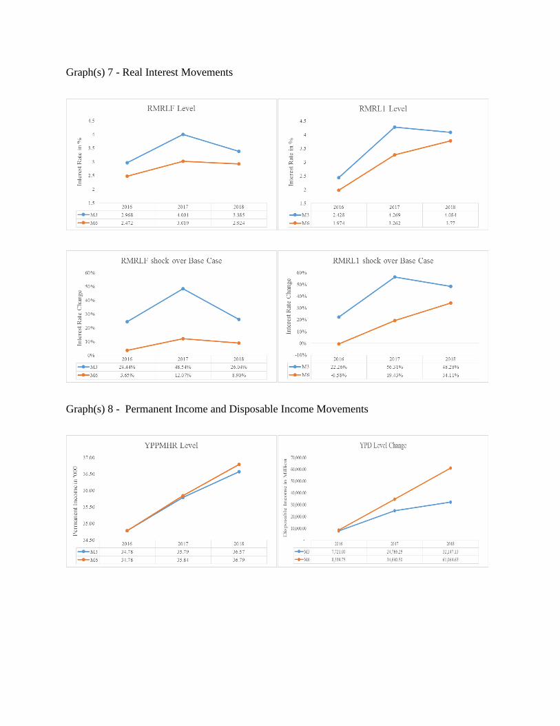
Graph(s) 7 - Real Interest Movements

Graph(s) 8 - Permanent Income and Disposable Income Movements

Graph(s) 9 - CPI and Unemployment Rate Movements

Graph(s) 10 - Exports and Imports Movements

Graph(s) 11 - Exchange Rate Movements