2015/2016, week 4 Cross-Country Income...
54
2015/2016, week 4 Cross-Country Income Differences Romer, Chapter 1.6, 1.7, 4.2, 4.5, 4.6
Transcript of 2015/2016, week 4 Cross-Country Income...

2015/2016, week 4Cross-Country Income Differences
Romer, Chapter 1.6, 1.7, 4.2, 4.5, 4.6

Differences in growth rates
Verdeling van inkomen en economische groei in geïndustrialiseerde landen
BBP per hoofd van
de bevolking, 1970
(in $)
BBP per hoofd van
de bevolking, 2009
(in $)
Economische groei
per jaar, 1970-2009
(in %)
VS 20.480 41.102 1,8
Nederland 19.050 40.566 2,0
Duitsland 16.236 32.487 1,8
Verenigd Koninkrijk 15.829 33.386 1,9
Frankrijk 15.676 30.821 1,7
Italië 14.371 27.692 1,7
Spanje 11.981 27.632 2,2
Zuid-Korea 3.018 25.029 5,6
Bron: Economen kunnen niet rekenen

Differences in growth rates
Verdeling van inkomen en economische groei in de wereld
Bron: Economen kunnen niet rekenen
BBP per hoofd van
de bevolking, 1970
(in $)
BBP per hoofd van
de bevolking, 2009
(in $)
Economische groei
per jaar, 1970-2009
(in %)
VS 20.480 41.102 1,8
Nederland 19.050 40.566 2,0
Venezuela 8.934 9.115 0,1
Madagascar 950 753 -0,6
India 886 3.238 3,4
China 865 7.431 5,7
Oeganda 817 1.152 0,9
Zimbabwe 339 143 -2,2

The power of economic growth
Suppose China, the Netherlands and Venezuela wereequivalent in terms of GDP 40 years ago
In 40 years, China growing 5.7 percent a year, wouldhave become 4 times as rich as the Netherlands
Similarly, in 40 years time, the Netherlands wouldhave become twice as rich as Venezuela growing 0.1percent a year only

Economic growth; scope and definition
Lecture is about structural economic growth
It is not about business cycle fluctations of growtharound its structural value
Economic growth refers to growth of the GrossDomestic Product
Homework
Environmental damage
Natural resources

Growth accounting
Adopts the concept of the aggregate productionfunction
Attributes economic growth to the contribution ofdifferent production factors

Growth accounting
Consider the aggregate production function
Take the total derivative of the above function withrespect to time:
�̇ � =��(�)
��(�)�̇ � +
�� �
�� ��̇ � +
�� �
�� ��̇ �
( ) ( ( ), ( ) ( ))Y t F K t A t L t

Growth accounting
Dividing both sides of the equation by �(�), we get
Which can be further simplified:
( ) ( ) ( ) ( ) ( ) ( ) ( ) ( ) ( ) ( )
( ) ( ) ( ) ( ) ( ) ( ) ( ) ( ) ( ) ( )
Y t K t Y t K t L t Y t L t A t Y t A t
Y t Y t K t K t Y t L t L t Y t A t A t
( ) ( ) ( ) ( )( ) ( )
( ) ( ) ( ) ( )K L
Y t K t L t A tt t
Y t K t L t A t

Growth accounting
Given that we have CRS, , we have thegrowth accounting equation:
An alternative formula is the following:
( ) ( ) ( ) ( ) ( )( ) (1 ( ))
( ) ( ) ( ) ( ) ( )K K
Y t L t K t L t A tt t
Y t L t K t L t A t
( ) 1 ( )K Lt t
( ) ( ) ( ) ( )( ) ( )
( ) ( ) ( ) ( )K
Y t L t K t L tt R t
Y t L t K t L t

Growth accounting
According to the growth accounting equation, economic growth is attributed to
Growth in the input of labour
Growth in the input of physical capital
The Solow residual: Technological progress
All other elements

Empirical application
Interesting application is Young (1995)
He adopts technique of growth accounting toexplain the extraordinary postwar growth of Hong Kong, Singapore, South Korea and Taiwan (Newly Industrializing Economies)

Empirical application
Result: economic growth has been high due to
Rising investment rates
Increasing labour force participation rates
Increasing levels of education
Intersectoral reallocations of labour towards the non-agricultural and manufacturing sector
Additionally, the contribution of other factors such as total factor productivity growth has been limited

Growth accounting: caveat
The factors that, according to growthaccounting, drive economic growth, may bedependent on one another
For example,
Labour force participation and education may bothbe related to labour productivity growth
Capital accumulation and also labour force participation may depend on technologicalprogress

Growth accounting: caveat
Hence, the technique of growth accounting may overstate on understate the contributionof a factor of production
For example, suppose increases withone percent
According to growth accounting, this increasesGDP with percent
If capital accumulation increases upon anincrease in the level of technology, the growtheffect is higher
( )A t
(1 ( ))K t

Growth accounting: caveat
Growth accounting can thus be used forlinking economic growth to different factors of production
Growth accounting should thus not be usedfor ‘what if’ simulation analysis

The Solow Growth model: the balanced growth path
Along the balanced growth path, Y/L and K/L grow at rate g
But g is exogenous
So the Solow model describes long-run growth by just imposing it!
In addition, the model is very abstract as regards the description of knowledge (or effectiveness of labour)

The Solow Growth model: convergence
The Solow Growth model predicts convergence to a state of balanced growth
Hence, countries starting below their long-run paths grow faster than those starting above
To see that consider a case where differences in Y/L stem only from physical capital per worker K/L. That is, human capital per worker and output for given inputs are the same across countries

The Solow Growth model: convergence
Assume again the CRS production function
Recall the adjustment equation for capital per effective worker:
measures the rate of convergence
* ( )i ik k k t
0
( ) ( ( ), ( ) ( ))Y t F K t A t L t

The Solow Growth model: convergence
This says that the farther is the economy below its balanced growth path, the faster does K/L grow
For Y/L a similar expression applies
Hence, also Y/L grows faster the more Y/L differs from its steady-state level

The Solow Growth model: convergence
As to the value of �∗, one can make two alternative assumptions
One is that �∗ is the same in all countries
In this case, all countries grow towards the same Y/L
The lower is the initial level Y/L, the faster is the growth of Y/L
We call this unconditional convergence

The Solow Growth model: convergence
A second assumption is that �∗ varies across countries
In this case, there is a persistent component of cross-country income differences
Poor countries (e.g., with low saving rates) may not grow faster than other countries
There is still convergence towards the own balanced growth path
We call this conditional convergence

The Solow Growth model: convergence
Unconditional convergence gives a good description of differences in growth among industrialized countries in the post-war period
This is so since saving rates, levels of education and other factors related to long-run fundamentals are similar across industrialized countries
For the same reason, it does not work that well for countries all over the world
In terms of the Solow Growth model, s, n and g can differ a lot between countries

Differences in growth rates
Verdeling van inkomen en economische groei in geïndustrialiseerde landen
BBP per hoofd van
de bevolking, 1970
(in $)
BBP per hoofd van
de bevolking, 2009
(in $)
Economische groei
per jaar, 1970-2009
(in %)
VS 20.480 41.102 1,8
Nederland 19.050 40.566 2,0
Duitsland 16.236 32.487 1,8
Verenigd Koninkrijk 15.829 33.386 1,9
Frankrijk 15.676 30.821 1,7
Italië 14.371 27.692 1,7
Spanje 11.981 27.632 2,2
Zuid-Korea 3.018 25.029 5,6
Bron: Economen kunnen niet rekenen

Differences in growth rates
Verdeling van inkomen en economische groei in de wereld
Bron: Economen kunnen niet rekenen
BBP per hoofd van
de bevolking, 1970
(in $)
BBP per hoofd van
de bevolking, 2009
(in $)
Economische groei
per jaar, 1970-2009
(in %)
VS 20.480 41.102 1,8
Nederland 19.050 40.566 2,0
Venezuela 8.934 9.115 0,1
Madagascar 950 753 -0,6
India 886 3.238 3,4
China 865 7.431 5,7
Oeganda 817 1.152 0,9
Zimbabwe 339 143 -2,2

Estimating convergence
Baumol (1986) addresses the question whether the growth performance of countries features convergence
Baumol (1986) examines convergence from 1870 to 1979 among 16 industrialized countries
He regresses output growth over this period on a constant and initial income
Model specification:

Estimating convergence
ln(Y/N) is log income per person, ε is an error term, and i indexes countries
Convergence if b <0: countries with higher initial incomes have lower growth
Perfect convergence if b = -1
No convergence if b = 0

Estimating convergence
Estimation result:

Estimating convergence
DeLong (1988) shows that Baumol’s finding islargely spurious, due to
Sample selection:
since historical data are constructed retrospectively, thecountries that have long data series are generally those thatare the most industrialized today
Measurement error:
estimates of real income per capita in 1870 are imprecise.Measurement error creates bias toward finding convergence

Estimating convergence
One way to tackle the first problem is to increase the sample and compare the richest countries as of 1870
DeLong (1988) creates a sample that consists of all countries at least as rich as the second poorest country in Baumol’s sample in 1870, Finland
Hence, he adds 7 countries (Argentina, Chile, East Germany, Ireland, New Zealand, Portugal, and Spain) and drops one (Japan)
Result:
the estimate of b of -0.995 drops to -0.566 and becomes less statistically significant

Estimating convergence
Way to tackle the second problem (i.e. measurementerror) is to estimate:

Estimating convergence
ln[(Y/N)1870]* is the true value of log income per capita in 1870
ln[(Y/N)1870] is the measured value
ε and u are assumed to be uncorrelated with each other and with ln[(Y/N)1870]∗
Result:
depending on the guess for the standard deviation of the estimation error, the estimate for b drops further, to 0 or even 1, thereby eliminating all of the remainder of Baumol’sestimate of convergence

Cross-country income differences: the role of capital
Where do income differences (i.e., differences in Y/L) between countries stem from?
Similarly, what makes income differ between time periods?
According to the Solow model, there are two candidate factors:
Differences in the capital per worker (K/L)
Differences in the effectiveness of labour (A)
Cross-country income differences: the role of capital
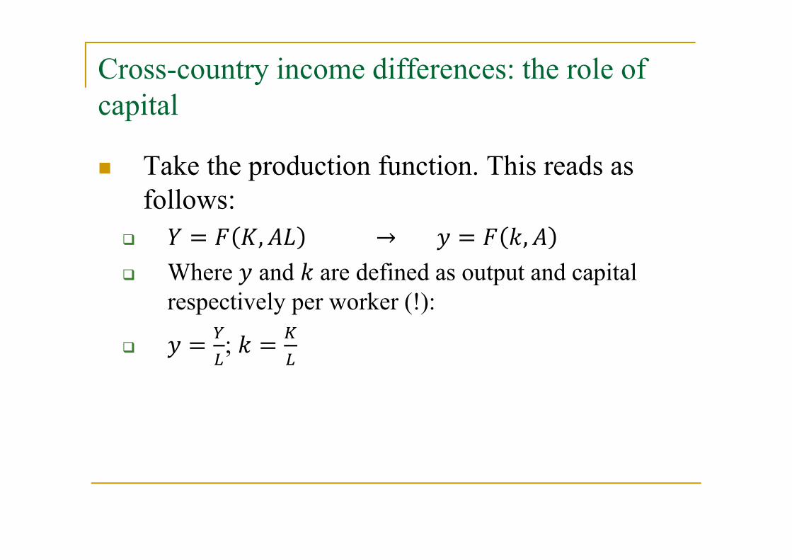
Take the production function. This reads as follows:
� = � �, �� → � = � �, �
Where � and �are defined as output and capital respectively per worker (!):
� =�
�; � =
�
�

Cross-country income differences: the role of capital
Assume the production function is Cobb-Douglas:
� = ��(��)���→
� = ������
Income difference between countries A and B:
� = ������
��
�� =��
��
���
��
���

Cross-country income differences: the role of capital
Can differences in the stocks of capital per worker explain income differences between countries?
In order to account for the difference in income between a rich country and a poor country of a factor 10, the stocks of capital need to differ a factor (10)�/�
Formally, solve ��
�� = 10 =��
��
�
→
��
�� = (10)�/�

Cross-country income differences: the role of capital
Standard elasticity of output w.r.t. capital
�=1/3: ��
�� = (10)�/(�
�)= 1000
Elasticity using broad measure of capital
�=1/2: ��
�� = (10)�/(�
�)= 100
Capital stocks differ not more than a factor 20 to 30 between rich and poor countries

Cross-country income differences: the role of capital
The marginal product of capital in the Cobb-Douglas case:
� = � � = �� →
�� � = ����� = ��(���)/�
In order to account for the difference in income between a rich country and a poor country of a factor 10, the marginal products of capital differ a factor (10)(���)/�

Cross-country income differences: the role of capital
Standard elasticity of output w.r.t. capital
�=1/3: ��(�)�
��(�)�= (10)(
��
�)/(
�
�)= 0.01
Elasticity using broad measure of capital
�=1/2: ��(�)�
��(�)�= (10)(
��
�)/(
�
�)= 0.1
Rates of return do not differ a factor 10 or 100 between countries
If they did so, we would observe massive capital flows from rich to poor countries

Income differences over time: the role of capital
For differences in income over time, the same holds true as for differences in income between countries:
In the data, capital stocks and rate of return on capital do not differ enough to account for the output differences
This implies
That countries and time periods differ a lot in terms of �
Or, that capital is much more valuable than is reflected in its price

Cross-country income differences: human capital
How about extending the approach by including human capital?
Would that increase the contribution from capital (and decrease the role of technology or, better, the residual)?
Take the following Cobb-Douglas production function
1( ) ( ) ( ( ) ( ))a aY t K t A t H t

Cross-country income differences: human capital
One can think of human capital H as the contribution of skills, expertise or education to the quality of labour
The more educated, skilled or experienced the labour force, the higher is human capital H

Cross-country income differences: human capital
To see how the introduction of human capital improves the ability of the model to explain income per capita growth and, hence, cross-country income differences, consider our new production function (in per capita terms) in logs
ln ln (1 ) ln (1 ) lni i ii
i i i
Y K Ha a a A
L L L

The above equation can be further rearranged as
����
��=
�
�����
��
��+ ��
��
��+ ����
Cross-country income differences: human capital
Cross-country income differences: human capital
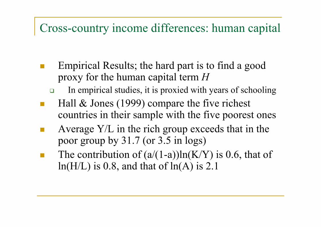
Empirical Results; the hard part is to find a good proxy for the human capital term H
In empirical studies, it is proxied with years of schooling
Hall & Jones (1999) compare the five richest countries in their sample with the five poorest ones
Average Y/L in the rich group exceeds that in the poor group by 31.7 (or 3.5 in logs)
The contribution of (a/(1-a))ln(K/Y) is 0.6, that of ln(H/L) is 0.8, and that of ln(A) is 2.1

Cross-country income differences: human capital
That is, only about a sixth in the gap between the richest countries and the poorest ones is due to differences in physical capital intensity
Only a slightly larger fraction is due to differences in schooling
The largest part of country differences in income per capita is due to differences in technology or other factors included in the Solow residual

Cross-country income differences: human capital
Extensions:
Human capital also depends on nationality worker (Klenowand Rodríguez-Claire 1997, Hendricks 2002)
Return to education may be different for different types of education
Low-skilled labour and high-skilled labour may be complements in production
Conclusion does not change:
The inclusion of human capital into the production function does not lead to dramatically different results

Cross-country income differences: the residual A
The fact that the residual term A is not well defined makes the empirical analysis tough. Why?
Because we want to know the determinants of growth. What are the determinants of economic growth? Are they exogenous or endogenously related to economic
policies? If so, which kind of economic policies?

Cross-country income differences: the residual A
A bunch of other possible factors exist that cancontribute to an explanation of economic growth
Charles Jones introduced the term socialinfrastructure
The whole of government activities that impact on thewedge between social and private returns
The definition is very broad: the activities may increase ordeteriorate social welfare

Cross-country income differences: social infrastructure
Taxation and subsidization of various activities (laboursupply, saving, investment, education) Operational costs
Costs in terms of changed economic behaviour
Costs in terms of an expansion of the informal economy
Legislation Crime
Enforceability of contracts
Government expropriation, bribery
Cross-country income differences: social infrastructure
Values and norms
Religion
Individual initiative
Interest groups
Dictatorship
Bribe-taking officials
Firms that benefit from a lack of competition

Cross-country income differences: geography
Average incomes in countries within 20 degrees of theequator are less than a sixth of those in countries at morethan 40 degrees of latitude
The former countries feature environments more conduciveto disease
The former countries feature climates less favourable toagriculture

Cross-country income differences: colonization strategies
Acemoglu, Johnson and Robinson argue thattoday’s institutions – which are important foreconomic growth – have been shaped bycolonization strategies as pursued by Europeancountries in the past few centuries
1 Establishment of “extractive states” that focus onexploitation without creating democratic institutions inhigh-mortality regions (Latin American countries)
2 Establishment of “settler colonies” that create institutionssimilar to those in the colonist countries in low-mortalityregions (United States, Australia, New Zealand)

Cross-country income differences: colonization strategies
Acemoglu and Robinson (2012), Why Nations Fail– The origins of power, prosperity and poverty
Book blends economics, politics and history
Argues that economic growth stems from inclusiveinstitutions
On the contrary, extractive institutions hindereconomic growth

Cross-country income differences: the residual A
The precise role of all these factors is still unknown,but currently widely investigated
Economists may fail to ever produce definitiveanswers to the question of the ultimate determinantsof economic growth on account of
a lack of empirical data
a lack of social experiments