2015, Vol. 16(3) 474–484 Real-time internal residual mass ...

Special Issue Article

International J of Engine Research2015, Vol. 16(3) 474–484� IMechE 2014Reprints and permissions:sagepub.co.uk/journalsPermissions.navDOI: 10.1177/1468087414552616jer.sagepub.com

Real-time internal residual massestimation for combustion with highcyclic variability

J Larimore1, E Hellstrom1, S Jade1, AG Stefanopoulou1 and Li Jiang2

AbstractIn this work, a physics-based method of estimating the residual mass in a recompression homogeneous charge compres-sion ignition engine is developed and analyzed for real-time implementation. The estimation routine is achieved throughin-cylinder pressure and exhaust temperature measurements coupled with energy and mass conservation laws appliedduring the exhaust period. Experimental results on a multicylinder gasoline homogeneous charge compression ignitionengine and dynamic analysis demonstrate the estimation routine’s ability to perform across a wide range of operatingconditions as well as on a cycle-by-cycle basis for highly variable combustion phasing data.

KeywordsHomogeneous charge compression ignition, residual gas fraction

Date received: 30 April 2014; accepted: 12 August 2014

Introduction

Autoignition timing control in homogeneous chargecompression ignition (HCCI) combustion requirescareful regulation of the temperature, pressure andcomposition of the pre-combustion cylinder charge.1,2

The regulation of charge properties is carried out inrecompression HCCI by retaining a large fraction ofthe post-combustion residual gases before they can beexhausted3,4 in addition to controlling the fuel injectiontiming.5–7 Accurate modeling of the residual gas frac-tion is important due to HCCI’s high sensitivity to thethermal energy associated with the residual gases.8–11 Iftoo much residual mass is trapped, the charge tempera-ture is too high and combustion occurs very early caus-ing a loss in efficiency and potential engine damage.12

If too little mass is trapped, the combustion becomesvery late and oscillatory.13,14 In the latter case, excessoxygen and unburned fuel can cause heat release dur-ing recompression which can result in efficiency loss,misfires, torque fluctuations and potential engine dam-age may occur.

Due to this sensitivity, it is desirable to estimate theresidual gas fraction online. There have been severalmethods described in the literature15–18 for offline esti-mation of the residual mass for steady-state conditions.This work presents a method of residual estimationwhich is computationally simple enough to be

implemented online while still maintaining a physicalbasis and alleviating the need of steady-state condi-tions. Analysis of the algorithm demonstrates fast con-vergence and the capability to handle high variabilitydata. Furthermore, a sensitivity analysis is providedwhich indicates that a tuning parameter can be used toaffect the dynamics and convergence of the algorithm.A block diagram of how the method works withrespect to cycle events is given in Figure 1.

The article is outlined as follows: first, an offlineresidual estimation technique is presented in section‘‘Iterative estimation.’’ In section ‘‘Real-time estima-tion’’ the method of section ‘‘Iterative estimation’’ ismodified for transients and online implementation. Insection ‘‘Dynamic analysis,’’ an analysis of the algo-rithm is performed to demonstrate its convergenceproperties and sensitivities. In section ‘‘Experimentalresults and setup,’’ the experimental setup is explained

1Department of Mechanical Engineering, University of Michigan, Ann

Arbor, MI, USA2Robert Bosch LLC, Denham, UK

Corresponding author:

J Larimore, Department of Mechanical Engineering, University of

Michigan, 3479 Burbank Dr. Ann Arbor, MI 48105, USA.

Email: [email protected]

at UNIV OF MICHIGAN on February 18, 2016jer.sagepub.comDownloaded from

http://jer.sagepub.com/

and the experimental results are provided; conclusionsare drawn in section ‘‘Conclusion.’’

Residual mass estimation

Crucial for proper combustion analysis is the determi-nation of residual mass. In section ‘‘Iterative estima-tion,’’ we derive an algorithm for trapped internalresidual mass in an engine operating with negative valveoverlap (NVO), following the method of Fitzgerald etal.15 Additionally, a modification to allow for highlyvariable data, as outlined in Larimore et al.,19 is pre-sented. This method is suitable for offline analysis.Furthermore, the formulation is modified to minimizethe effects of steady-state assumptions and simplify thealgorithm for real-time implementation in section‘‘Real-time estimation.’’

Iterative estimation

The trapped residual mass (mres) is defined as the in-cylinder charge at the time of exhaust valve closing(EVC) and is based on the ideal gas law mres=PevcVevc/RTevc. The in-cylinder pressure is measured,which provides Pevc and the cylinder volume at EVC,Vevc, is known. The gas constant is for a burned gascomposition and is assumed constant and known,R=290(J=kgK). Therefore, to determine the residualmass, Tevc must be estimated. To do so, a system ofequations is developed from which Tevc, and conse-quently mres, may be determined.

In steady-state conditions, the mass flowing out ofthe cylinder during the exhaust stroke, mout, is equal tomass of fresh air and fuel, mair and mf, respectively,inducted into the cylinder within a given cycle

mout =mair+mf =min ð1Þ

The mass that leaves through the exhaust process(exhaust valve opening (EVO) ! EVC) can bedescribed as

PevoVevo

RTevo� PevcVevc

RTevc=mair+mf ð2Þ

where the pressures at the valve events, Pevo and Pevc,are measured, as are mair and mf. Equation (2) has twounknowns, Tevo and Tevc; therefore, an additional rela-tion is needed to solve for the unknown temperatures.

In addition to the steady-state conservation of massin equation (2), the exhaust process can be approxi-mated by an ideal gas undergoing a reversible process.The heat loss per unit mass, during the crank angleinterval u0!u1, is given by

ql(u0, u1)=

ðT(u1)T(u0)

cpdT� R

ðP(u1)P(u0)

T

PdP ð3Þ

where cp is the specific heat of the exhaust gas which isassumed constant and known. The exhaust process issplit into two parts, a blowdown phase and compres-sion phase. The ratio of the heat losses for these twophases is denoted by rex

rex=ql(uevo, uref)

ql(uref, uevc)ð4Þ

The point used to split the exhaust process, uref, isreferred to as the reference point. In Fitzgerald et al.,15

it is the point when exhaust runner pressure is equal to1 atm. To accommodate boosted conditions, one couldinstead use the point of minimum pressure as inHellstrom et al.20 However, in highly variable condi-tions, the minimum could occur close to the valveevents. For example, it was observed that the minimummay be at EVO following misfires, see Figure 2. Toavoid possible numerical issues associated with this sce-nario, the reference point is fixed in the middle of thevalve open period, uref=(uevo+ uevc)=2.

By combining equations (3) and (4), with simplifica-tions from Fitzgerald et al.,15 we arrive at the equation

(cp + a)Tevo+(cp � b)rex

Tevc =Tref cp � a+(cp + b)rex� �

ð5Þ

where a=1=2R log Pref=Pevo and b=1=2R logPevc=Pref. The variables Tref and Pref are the measuredexhaust gas temperature and in-cylinder pressure aturef, respectively.

The heat loss ratio rex is estimated by convective heattransfer to the walls as governed by

dQl

dt=Ahc(Tcyl � Tw) ð6Þ

where the heat transfer coefficient, hc, is determinedusing the Woschni method from Heywood,21 and A isthe cylinder area. A constant wall temperature, Tw, is

Figure 1. A block diagram representation of the inputs andoutputs of the online residual mass estimation.

Larimore et al. 475



assumed and the in-cylinder temperature, Tcyl, is obtainedusing a polytropic process. The result of equation (6) issubstituted into equation (4) to yield the heat loss ratio asa function of the temperature at the valve events

rex = f(Tevo,Tevc) ð7Þ

In summary, equations (2), (5) and (7) are threeequations with three unknowns Tevo, Tevc and rex. Dueto the nonlinear relationship in equation (7), the solu-tion is found numerically. For a given rex, equations (2)and (5) are solved for (Tevo, Tevc). Inserting the solu-tions into equation (7) gives an implicit relation that issolved numerically. The fixed-point iteration,rex(k + 1)= f(Tevo(rex(k)), Tevc(rex(k))), rex(0)=1, wasa fast method of solutions, typically only five iterationswere required for convergence in most datasets with atermination condition of jrex(k)2 rex(k2 1)j \ 1024.With the solution (rex, Tevo, Tevc), the mass of residualsmay be found with the ideal gas law. The residual gasfraction is then determined by

xr =mres

mair+mf +mres=

PevcVevcTevo

PevoVevoTevcð8Þ

Despite the fast convergence of this routine, it is tooslow for implementation in an industrial engine controlunit (ECU). To alleviate the need for iterations, wecould instead fix the value of rex as a constant.

It can be hypothesized that the value of rex will begreater than 1. This is due to the fact that blowdown, aprocess in which a large amount of heat is lost due to arapid equalization of pressure between the exhaustmanifold and cylinder, occurs in the first part of theexhaust process and the fact that we have defined thetwo portions of equation (4) to be of equal length. Theexact value of this ratio is unknown without the

iterative process previously described. However, theiterative analysis supports this claim where the averagevalue across multiple operating conditions is rex=1.5.The effect of rex on the final result is small, as will beshown section ‘‘Sensitivity.’’ It could therefore be dele-gated as a tuning factor; for this analysis, it is assumeda known constant.

Real-time estimation

Residual gas fraction was determined using the iterativeapproach in section ‘‘Iterative estimation’’ is suitablefor offline analysis; however, the iterative nature limitsits use for real-time estimation. The iterations of thisalgorithm were eliminated by assigning the variable rexto a fixed value. However, the method is still not suit-able for real-time estimation on an actual enginebecause it is restricted to steady state.

In section ‘‘Iterative estimation,’’ steady state wasassumed through conservation of mass in equation (1).To provide flexibility in this assumption, the unknowntemperatures of equation (2) can instead be definedwith the ideal gas law

Tevo=PevoVevo

mevoRð9Þ

Tevc=PevcVevc

mevcRð10Þ

and the masses can be defined by

mevo=min(k)+mres(k) ð11Þ

mevc=mres(k+1) ð12Þ

Equation (11) tells us that the mass of charge at uevois equal to the mass of inducted air and fuel as well asthe mass of residuals from the current cycle. After theexhaust process is complete, the mass at the time of uevcis equivalent to the mass of residual trapped for thenext cycle, according to the cycle definition of Figure 1.This formulation provides flexibility during non-stationary conditions as it allows mres to evolve in timefollowing real-time measurements of Tex and Pcyl. Themeasurement of Tex is achieved with a thermocouple inthe exhaust runner port in this work. This could bereplaced with a model, or a fast sensor, in future workto mitigate the potential issue of slow thermocoupleresponse times. The in-cylinder pressure sensor, how-ever, is capable of responding on a crank angle resolu-tion basis. The algorithm carries a high sensitivity toPcyl and a moderate sensitivity to Tex as will be dis-cussed further in section ‘‘Sensitivity.’’

Equations (5), (9) and (10) can then be combinedand written as

(cp + a)PevoVevo

min(k)+mres(k)ð ÞR +(cp � b)rexPevcVevc

mres(k+1)R

=Texfcp � a+(cp + b)rexg ð13Þ

Figure 2. Minimum in the in-cylinder pressure trace can beseen to occur at EVO for some cycles in highly variable data withmisfires as shown in gray. This is contrary to normal combustion,in black, where the minimum is typically close to the middle.EVO: exhaust valve opening; EVC: exhaust valve closing.

476 International J of Engine Research 16(3)



Equation (13) can be written more compactly bygrouping terms and lumping constant coefficients

mres(k+1)=a(k)+b(k)mres(k)

A(k)+mres(k)ð14Þ

where

a(k)=rex(b� cp)

cp � a+(cp + b)rex

� �PevcVevc

RTex

� �min(k)

b(k)=rex(b� cp)


� �PevcVevc

RTex

� �

A(k)=cp + a


� �PevoVevo

RTex

� �+min(k)

The values of Px, Tx and Vx are all from the k + 1cycle. Equation (14) predicts the amount of residualmass in cycle k + 1 based on previous measured dataand the value of the residual mass on the previouscycle. Therefore, the only unknown is the initial guessof mres(0). It will be shown in the following sectionsthat regardless of the initial guess, the difference equa-tion will converge relatively quickly to a stable equili-brium. A limitation of the algorithm is that it requiresa transient air mass as an input. Figure 1 provides avisual representation of this algorithm and its inputsrelative to the cycle definition at EVO.

Undefined sets. Due to the fact that equation (14) isrational, there are sets of values (a, b, A) for which thedifference equation is undefined, namely, when divisionby 0 occurs. The conditions are unphysical in nature;however, it is important that we consider these possibi-lities to understand any numerical issues that may arise.For the following analysis, rex is assumed to be equalto 1 for mathematical simplicity. Division by 0 occurswhen

A+mres(k)=0! mres(k)= � A

This scenario is obviously unphysical and can beavoided by picking a positive initial guess of residualmass. If mres(k) . 0, then mres(k + 1) . 0; this is dis-cussed further in section ‘‘Convergence.’’

Another possible numerical issue occurs whena=bA. This causes a single solution for all cycles

mres(k+1)=bA+bmres(k)

A+mres(k)=b 8 k50

Essentially, the algorithm could become ‘‘stuck’’ onthis solution if there were no changes in the coefficients.However, if we evaluate the term a 2 bA=0, we seethat for this to be true

2cp +R lnPref

Pevo

� ��4cp +R ln

P2ref

PevoPevc

� �0B@

1CA PevoVevo

RTex

� �=0

Since we know the ratio inside the natural log isalways close to 1, the value of the logarithm is close to

0. Additionally, PevoVevo can never equal 0 and thevalue of 2cp is always positive so it is unlikely thisexpression is ever true.

Dynamic analysis

In a stationary condition, it is important to investi-gate the existence of an equilibrium and the potentialmultiplicity issue. Additionally, it is important tounderstand the nature of convergence to an equili-brium for transient conditions. In the following sec-tions, an analysis of equation (14) will be performedfor which the coefficients a, b and A will be assumedconstant. Specifically, a proof that equation (14)has two fixed-point solutions for a given set of inputsis provided in section ‘‘Existence of two solutions’’and an analysis that shows that the algorithm con-verges to a physical solution is given in section‘‘Convergence.’’ A sensitivity analysis is performed insection ‘‘Sensitivity.’’

Existence of two solutions

An equation in the form of equation (14) is well knownin mathematics as the Riccati difference equation, asshown in Kulenovic and Ladas.22 Since the equation isrational and of second order, it can have at most twosolutions; these solutions can be real or imaginary. It isimportant to understand what these solutions are for agiven set of input data and the stability of eachsolution.

To find the two solutions, we impose a change invariables such that

mres(k)= (b+A)w(k)� A 8 k50

and substituting this into equation (14), we then havethe difference equation

w(k+1)=1� Q

w(k)where Q=

bA� a

(b+A)2ð15Þ

At steady state, w(k + 1)=w(k)=w, the expres-sion can be written as w22w + Q=0. This is an easilysolved quadratic equation that yields the two possiblesolutions

w�=1�

ffiffiffiffiffiffiffiffiffiffiffiffiffiffiffi1� 4Qp

2and w+ =

1+ffiffiffiffiffiffiffiffiffiffiffiffiffiffiffi1� 4Qp

2

ð16Þ

If Q\ 1=4, then equation (15) has two real solu-tions. If Q. 1=4, then there are two imaginary solu-tions, and if Q=1=4 then the solutions arew�=w+ =1=2.

To prove this equation always has these two solu-tions, we can show the value of Q is less than 1/4 and isnegative for any physically reasonable set of pressuredata. To do this, we examine the sign of Q. We mayfirst exclude the denominator because it is squared andwill always be positive. Therefore, the sign of Q is

Larimore et al. 477



dictated by the sign of the numerator alone. Thenumerator, bA2 a, can be rearranged asb(A2min(k)), which can be evaluated in detail as

b A�min(k)ð Þ= PevcVevcPevoVevo

R2T2ex

� �

�2cp +R ln Pevc

Pref

� �� 2cp +R ln

Pref

Pevo

� �� 4cp +R ln

P2ref

PevoPevc

� �� 20B@

1CA

From this, we can see that the sign of Q is deter-mined by

�2cp +R lnPevc

Pref

� �� 2cp +R ln

Pref

Pevo

� ��

since the term (PevcVevcPevoVevo) is always positive.Expansion of terms yields

� 4c2p +2cpR lnPevcPevo

P2ref

!+R2 ln

Pevc

Pref

� �ln

Pref

Pevo

� �

ð17Þ

The sign of this term dictates the sign of Q. To findthe sign of this term, we must apply some constraintson the pressures. We know during the exhaust processPevo, Pevc and Pref are all very close to one another,therefore

PevcPevo

P2ref

’Pevc

Pref’

Pref

Pevo’1

Because of this, the last two terms of equation (17)are very close to 0 and are small by comparison to thefirst term, which is always negative. In fact, for equa-tion (17) to become positive, the pressure ratios insidethe natural logs would all have to be greater than 20.Since exhaust pressures are usually around 1 bar andnot more than 5 bar for most applications, pressureratios of this magnitude are not feasible. We can there-fore conclude the sign of Q is always negative for physi-cally reasonable data and there will always be twosolutions, w2 and w+, given by equation (16). Usingthis same argument, we can support the claim in sec-tion ‘‘Real-time estimation’’ that a 2 bA is not equal to0. The preceding argument shows bA2 a is always lessthan 0.

Convergence

Equation (14) predicts the amount of residual mass incycle k + 1 based on measured data and the value ofthe residual mass in the previous cycle. Therefore, theonly unknown is the initial guess of mres(0). Since weknow the equation has two fixed-point solutions, asshown in section ‘‘Existence of two solutions,’’ it isdesirable to know how the equation converges to thesesolutions and if the solutions are stable.

If typical values of a, b and A are used in the resi-dual mass estimation and held constant, the changefrom one cycle to the next can be determined from thediscrete derivative of equation (14).

An example of this is shown in Figure 3 for initialconditions ranging from 21000 to 1000mg. Here, theequation has equilibria at 294.4 and 220.9mg. Clearly,the negative solution is non-physical as we cannot havea negative mass. If we linearize the function at eachone of the equilibria, we find that the slope at the nega-tive solution is outside the criteria for a stable equili-brium. Specifically, if the solution was stable, the slopeat the solution would be 21 \ m \ 1, where m is theslope of the function at a particular point. The slope atthe positive solution is 20.57, and this equilibrium istherefore stable and oscillatory. As such, an initial con-dition that is close to stable equilibria will converge tothe positive solution for this set of coefficients. The fig-ure shows how an initial guess of mres(0)=0 wouldconverge to the stable equilibrium in blue. Further sta-bility properties of the Riccati difference equation canbe found in Kulenovic and Ladas,22 Grove et al.23 andSedaghat.24

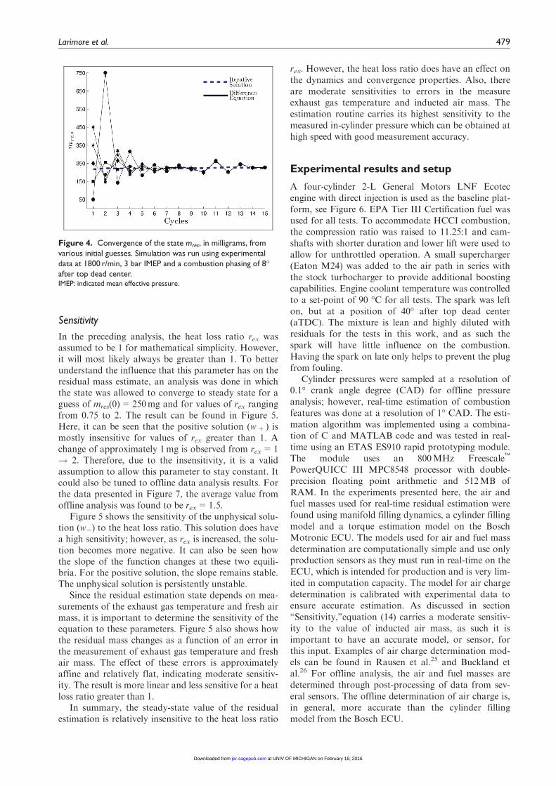
Figure 4 highlights the evolution of convergencefrom various positive initial guesses. In this case, theinitial guess was purposely chosen to be far away fromthe actual value to demonstrate the nature of conver-gence at various conditions. In real operation, the ini-tial guess is chosen to be more physically reasonableand close to the actual value. It can be seen here thatthe equation converges to the same predicted residualmass within a small number of cycles. Additionally, itconverges to approximately the same value as a higherfidelity offline analysis tool.15

Figure 3. Change in the value of the estimated mres, inmilligrams, from one cycle to the next. Two fixed-point solutionsare shown and the slop at each point indicates the solutionsstability.




Sensitivity

In the preceding analysis, the heat loss ratio rex wasassumed to be 1 for mathematical simplicity. However,it will most likely always be greater than 1. To betterunderstand the influence that this parameter has on theresidual mass estimate, an analysis was done in whichthe state was allowed to converge to steady state for aguess of mres(0)=250mg and for values of rex rangingfrom 0.75 to 2. The result can be found in Figure 5.Here, it can be seen that the positive solution (w+) ismostly insensitive for values of rex greater than 1. Achange of approximately 1mg is observed from rex=1! 2. Therefore, due to the insensitivity, it is a validassumption to allow this parameter to stay constant. Itcould also be tuned to offline data analysis results. Forthe data presented in Figure 7, the average value fromoffline analysis was found to be rex=1.5.

Figure 5 shows the sensitivity of the unphysical solu-tion (w2) to the heat loss ratio. This solution does havea high sensitivity; however, as rex is increased, the solu-tion becomes more negative. It can also be seen howthe slope of the function changes at these two equili-bria. For the positive solution, the slope remains stable.The unphysical solution is persistently unstable.

Since the residual estimation state depends on mea-surements of the exhaust gas temperature and fresh airmass, it is important to determine the sensitivity of theequation to these parameters. Figure 5 also shows howthe residual mass changes as a function of an error inthe measurement of exhaust gas temperature and freshair mass. The effect of these errors is approximatelyaffine and relatively flat, indicating moderate sensitiv-ity. The result is more linear and less sensitive for a heatloss ratio greater than 1.

In summary, the steady-state value of the residualestimation is relatively insensitive to the heat loss ratio

rex. However, the heat loss ratio does have an effect onthe dynamics and convergence properties. Also, thereare moderate sensitivities to errors in the measureexhaust gas temperature and inducted air mass. Theestimation routine carries its highest sensitivity to themeasured in-cylinder pressure which can be obtained athigh speed with good measurement accuracy.

Experimental results and setup

A four-cylinder 2-L General Motors LNF Ecotecengine with direct injection is used as the baseline plat-form, see Figure 6. EPA Tier III Certification fuel wasused for all tests. To accommodate HCCI combustion,the compression ratio was raised to 11.25:1 and cam-shafts with shorter duration and lower lift were used toallow for unthrottled operation. A small supercharger(Eaton M24) was added to the air path in series withthe stock turbocharger to provide additional boostingcapabilities. Engine coolant temperature was controlledto a set-point of 90 �C for all tests. The spark was lefton, but at a position of 40� after top dead center(aTDC). The mixture is lean and highly diluted withresiduals for the tests in this work, and as such thespark will have little influence on the combustion.Having the spark on late only helps to prevent the plugfrom fouling.

Cylinder pressures were sampled at a resolution of0.1� crank angle degree (CAD) for offline pressureanalysis; however, real-time estimation of combustionfeatures was done at a resolution of 1� CAD. The esti-mation algorithm was implemented using a combina-tion of C and MATLAB code and was tested in real-time using an ETAS ES910 rapid prototyping module.The module uses an 800MHz Freescale�

PowerQUICC III MPC8548 processor with double-precision floating point arithmetic and 512MB ofRAM. In the experiments presented here, the air andfuel masses used for real-time residual estimation werefound using manifold filling dynamics, a cylinder fillingmodel and a torque estimation model on the BoschMotronic ECU. The models used for air and fuel massdetermination are computationally simple and use onlyproduction sensors as they must run in real-time on theECU, which is intended for production and is very lim-ited in computation capacity. The model for air chargedetermination is calibrated with experimental data toensure accurate estimation. As discussed in section‘‘Sensitivity,’’equation (14) carries a moderate sensitiv-ity to the value of inducted air mass, as such it isimportant to have an accurate model, or sensor, forthis input. Examples of air charge determination mod-els can be found in Rausen et al.25 and Buckland etal.26 For offline analysis, the air and fuel masses aredetermined through post-processing of data from sev-eral sensors. The offline determination of air charge is,in general, more accurate than the cylinder fillingmodel from the Bosch ECU.

Figure 4. Convergence of the state mres, in milligrams, fromvarious initial guesses. Simulation was run using experimentaldata at 1800 r/min, 3 bar IMEP and a combustion phasing of 8�after top dead center.IMEP: indicated mean effective pressure.

Larimore et al. 479



Comparison to steady-state data

To validate the online residual estimation’s accuracy, itwas compared to the results from the offline estimationpresented in section ‘‘Iterative estimation.’’ Ideally, theresults from the online analysis would be comparedagainst measurements of the residual mass.Unfortunately, sampling of the in-cylinder charge isextremely difficult; it has, however, been done inSteeper and Davisson.27 This method, however,requires steady-state operation and the engine cannotcontinue to run once a sample has been taken.

The dataset used for comparison spans multiplespeeds, loads and actuator settings and is therefore rep-resentative of the range of inputs that the equationwould receive when operating online. The results inFigure 7 show that for values of rex=1, the fit is good

Figure 5. Sensitivity of the residual mass to errors in the measured exhaust gas temperature. The sweeps are performed forvarious heat loss ratios, and the results are linear for a physically reasonable value of rex.

Figure 6. Multicylinder recompression HCCI engine used fortesting along with all rapid prototyping hardware andinstrumentation.




with the exception of a few outliers. The outliers corre-spond to higher load points. For these, the pressure inthe cylinder at the point of EVO was high due to higherpeak pressures. The result is a larger blowdown eventwhich would make the value of rex necessarily greaterthan 1. The results are better when a heat loss ratiogreater than 1 is used and nearly identical to the offlineanalysis when the value of rex from the iterative methodis used. This comparison of the data was made offline.

Cycle-by-cycle trends

Since the residual mass trapped in the cylinder canchange quickly on a cycle-by-cycle basis, it is importantto quantify how well the algorithm can capture thesefluctuations. Figure 8 shows the result of the online dif-ference equation and offline analysis for a highly vari-able dataset. These data were made variable by

reducing the amount of NVO and therefore trappedresidual mass such that the combustion phasingbecame sufficiently late to induce oscillations in thecombustion phasing and cylinder pressure.14 Figure 8shows that the online estimation well approximates theoffline result in terms of direction of change from onecycle to the next in the presence of this high variabilityin Pcyl. However, it is possible that in the extreme vaseof frequent misfires that the algorithm could saturateand have difficulty converging back to a solution.

The standard deviation of the online result is higherthan that of the offline. This is due to the oscillatoryconvergence of the online estimation. When a heat lossratio greater than 1 is used, the amplitude of oscilla-tions is reduced. This is the same result deduced fromFigure 5 where we see that the slope of the function atthe physical solution is approaching 0 as the heat lossratio is increased. This slope is analogous to the eigen-value of the system. In discrete time, an eigenvalue onthe left-half plane and inside the unit circle is stable butoscillatory. As we move the eigenvalue closer to posi-tive values, the dampening of the system increases.Additionally, errors could result from the differentmeans by which the cycle-by-cycle air mass is deter-mined. For the online solution, the air mass is deter-mined using the Bosch ECU and a cylinder fillingmodel as outlined in section ‘‘Experimental results andsetup.’’

To further check the statistical properties of thealgorithm, we consider the full test from Figure 8 whichis 3000 cycles long. The results are presented in Figure9 with return maps and normal probability plots. Areturn map shows the relationship between consecutivecycles which provides insight on the dynamic behaviorof the cyclic variability (CV). Here, the return map isthe plot of the residual mass in cycle k versus the resi-dual mass in cycle k + 1. When comparing the onlineand offline results, we can see that the online analysisresults are stretched slightly perpendicular to the diago-nal indicating oscillatory behavior. This is most likelycaused by the heat loss ratio being tuned slightly low asprevious results would indicate. The results for bothcases are mostly Gaussian as indicated by the normalprobability plots.

Even though the residual gas fraction data in Figure9 appears to have fairly low variability, the effect on thecombustion is actually significant and non-Gaussian.This is made clear by the return maps of combustionphasing and heat release in Figure 10.

Actuator steps

To evaluate the effectiveness of the residual gas fractionestimation in transients, actuator steps of the modelinputs were performed in open loop. Sensor measure-ments were obtained in real-time from the engine’sECU and used by the model for real-time prediction ofxr. A step in EVC is shown in Figure 11 for cylinder 1.The step is from 256� to 253� aTDC and back again

Figure 7. Comparison of the online residual estimation withthat of an iterative offline analysis tool from Fitzgerald et al.15.

Figure 8. Cycle-resolved results of residual mass for differentvalues of rex. Despite the data’s high variability, the algorithmcaptures cycle-by-cycle trends well. The increased value of rex

dampens oscillations.

Larimore et al. 481



and causes the amount of NVO to increase as a result.Intuitively, the amount of residual mass trapped in thecylinder should also increase; this is reflected in the pre-diction of the residual gas fraction. The EVC step issmall because this is the largest step change that can beachieved in open loop at this particular operating con-dition. Without compensation from other actuators,

the engine transitions between nearly misfiring andringing with this slight change in residual gas fractionas seen by the response of combustion phasing inFigure 11. Also shown is the result of the offline analy-sis of the residual gas fraction from Fitzgerald et al.15

and Larimore et al.19 While the absolute differencebetween the two results is not 0, the magnitude and

Figure 9. Return maps and normal probability plots of the online and offline residual estimation for a highly variable dataset.

Figure 10. Return maps of heat release and combustion phasing for the data presented in Figure 9. Here, it can be seen thatdespite the low variability in the return maps of residual gas fraction, the combustion is erratic in terms of u50 and heat release.




direction of the transient response are similar. Theabsolute value of the two results differs due to the dif-ferent methods used to calculate the inducted air massas discussed in section ‘‘Experimental results andsetup.’’

Conclusion

A physics-based method of estimating the trapped resi-dual mass in a recompression engine using cylinderpressure measurements has been presented and evalu-ated through dynamic analysis and experiments. Anaccurate estimation of residual mass is important tounderstand and control HCCI dynamics due to its largesensitivity to thermal properties of the charge mass. Inrecompression HCCI, the charge temperature is mostdirectly effected by the trapped residual mass.

The algorithm is viable for real-time implementationdue to its simplicity and it has been shown that the esti-mation is valid for highly variable datasets. This is dueto the algorithm’s ability to converge quickly from per-turbations. Furthermore, an analysis has been done toshow sensitivity properties to a tuning parameter andmeasurement errors. The tuning parameter rex has littleinfluence on the steady-state result but does impact thedynamics and convergence of the algorithm. A limita-tion of the algorithm is that it requires a transient airmass as an input. The results from the residual

estimation are sensitive to errors in this input as indi-cated by Figure 5 and so it is imperative that a well-parameterized charge determination model is usedwhen implementing the algorithm online.

Declaration of conflicting interests

This report was prepared as an account of work spon-sored by an agency of the US Government. Neither theUS Government nor any agency thereof, nor any oftheir employees, makes any warranty, express orimplied, or assumes any legal liability or responsibilityfor the accuracy, completeness, or usefulness of anyinformation, apparatus, product, or process disclosed,or represents that its use would not infringe privatelyowned rights. Reference herein to any specific commer-cial product, process, or service by trade name, trade-mark, manufacturer, or otherwise does not necessarilyconstitute or imply its endorsement, recommendation,or favoring by the US Government or any agencythereof. The views and opinions of authors expressedherein do not necessarily state or reflect those of theUS Government or any agency thereof.

Funding

This material was supported by the Department ofEnergy (National Energy Technology Laboratory) DE-EE0003533 as a part of the ACCESS project consor-tium with direction from Hakan Yilmaz and OliverMiersch-Wiemers, Robert Bosch, LLC.

References

1. Olsson JO, Tunestal P and Johansson B. Closed-loop

control of an HCCI engine. SAE paper 2001-01-1031,

2001.2. Shaver GM and Gerdes JC. Cycle to cycle control of

HCCI engines. In: Proceedings of IMECE 2003,

Washington, DC, 15–21 November 2003, IMECE2003-

41966. ASME Technical Publishing Office, NY.3. Yao M, Zheng Z and Liu H. Progress and recent trends

in HCCI engines. Prog Energ Combust 2009; 35(5):

398–437.4. Willand J, Nieberding RG, Vent G and Enderle C. The

knocking syndrome—its cure and its potential. SAE

paper 982483, 1998.5. Roelle MJ, Jungkunz AF, Ravi N and Gerdes JC. A

dynamic model of recompression HCCI combustion includ-

ing cylinder wall temperature. In: Proceedings of IMECE

2006, Chicago, IL, 5–10 November 2006, IMECE2006-

15125. ASME Technical Publishing Office, NY.6. Wermuth N, Yun H and Najt P. Enhancing light load

HCCI combustion in a direct injection gasoline engine

by fuel reforming during recompression. SAE Int J

Engines 2009; 2: 823–836.7. Marriott C and Reitz R. Experimental investigation of

direct injection-gasoline for premixed compression

ignited combustion phasing control. SAE paper 2002-01-

0418, 2002.8. Chiang CJ and Stefanopoulou AG. Stability analysis in

homogeneous charge compression ignition (HCCI)

Figure 11. An EVC step for cylinder 1. The online residual gasfraction prediction (black) is compared against the offlineprediction (red). The cycle-by-cycle predictions are goodthroughout the test; however, there is an offset in the meanvalue most likely caused by a difference in the estimation ofmass of air. The step is small because an open-loop EVC stephas a large effect on the combustion phasing.EVC: exhaust valve closing; aTDC: after top dead center.

Larimore et al. 483



engines with high dilution. IEEE T Contr Syst T 2007;15(2): 209–219.

9. Daw CS, Wagner RM, Edwards KD Jr and JohneyBGJr. Understanding the transition between conven-tional spark-ignited combustion and HCCI in a gasolineengine. P Combust Inst 2007; 31(2): 2887–2894.

10. Kulzer A, Lejsek D, Kiefer A and Hettinger A. Pressuretrace analysis methods to analyze combustion featuresand cyclic variability of different gasoline combustionconcepts. SAE paper 2009-01-0501, 2009.

11. Shahbakhti M and Koch CR. Characterizing the cyclicvariability of ignition timing in a HCCI engine fueledwith n-heptane/iso-octane blend fuels. Int J Engine Res

2008; 9(5): 361–397.12. Manofsky L, Vavra J, Assanis D and Babajimopoulos A.

Bridging the gap between HCCI and SI: spark-assistedcompression ignition. SAE paper 2011-01-1179, 2011.

13. Hellstrom E, Stefanopoulou AG and Jiang L. Cyclicvariability and dynamical instabilities in autoignitionengines with high residuals. IEEE T Contr Syst T 2013;21(5): 1527–1536.

14. Hellstrom E, Larimore J, Sterniak J, Jiang L and Stefa-nopoulou A. Quantifying cyclic variability in a multi-cylinder HCCI engine with high residuals. J Eng Gas

Turb Power 2012; 134: 112803.15. Fitzgerald RP, Steeper R, Snyder J, Hanson R and Hessel

R. Determination of cycle temperature and residual gasfraction for HCCI negative valve overlap operation. SAEInt J Engines 3: 124–141 (2010-01-0343).

16. Mladek M and Onder C. A model for the estimation ofinducted air mass and the residual gas fraction usingcylinder pressure measurements. SAE Int 2000; 1: 1–11(2000-01-0958).

17. Gazis A, Panousakis D, Patterson J, Chen HW, Chen Rand Turner J. Using in-cylinder gas internal energy bal-ance to calibrate cylinder pressure data and estimate resi-dual gas amount in gasoline HCCI combustion. Exp

Heat Transfer 2008; 21(4): 275–280.

18. Ortiz-Soto EA, Vavra J and Babajimopoulos A. Assessmentof residual mass estimation methods for cylinder pressureheat release analysis of HCCI engines with negative valveoverlap. In: Proceedings of ASME 2011 internal combustion

engine division fall technical conference, Morgantown, WV,2–5 October 2011. ASME Technical Publishing Office, NY.

19. Larimore J, Hellstrom E, Sterniak J, Jiang L and Stefano-poulou A. Experiments and analysis of high cyclic varia-bility at the operational limits of spark-assisted HCCIcombustion. In: Proceedings of the American control con-

ference (ACC), Montreal, QC, Canada, 27–29 June 2012,pp.2072–2077. New York: IEEE.

20. Hellstrom E, Stefanopoulou AG, Vavra J, Babajimopou-los A, Assanis D, Jiang L and Yilmaz H. Understandingthe dynamic evolution of cyclic variability at the operat-ing limits of HCCI engines with negative valve overlap.SAE Int J Engines 2012; 5(3): 995–1008.

21. Heywood J. Internal combustion engine fundamentals.McGraw-Hill Science/Engineering/Math, 1988, NY.

22. Kulenovic MRS and Ladas G. Dynamics of second order

rational difference equations with open problems and conjec-

tures. Boca Raton, FL: Chapman and Hall/CRC, 2002.23. Grove EA, Ladas G, McGrath LC and Teixeira CT.

Existence and behavior of solutions of a rational system.Commun Appl Nonlin Anal 2001; 8(1): 1–25.

24. Sedaghat G. Existence of solutions of certain singular dif-ference equations. J Differ Equ Appl 2000; 6(5): 535–561.

25. Rausen DJ, Stefanopoulou AG, Kang JM, Eng JA andKuo TW. A mean value model for control of HCCIengines. J Dyn Syst: T ASME 2005; 127(3): 355–362.

26. Buckland J, Jankovic M, Grizzle J and Freudenberg J. Esti-mation of exhaust manifold pressure in turbocharged gaso-line engines with variable valve timing. In: Proceedings of

dynamic systems and control conference, Ann Arbor, MI, 20–22 October 2008. ASME Technical Publishing Office, NY.

27. Steeper RR and Davisson ML. Analysis of gasolinenegative-valve-overlap fueling via dump sampling. SAEInt J Engines 2014; 7: 762–771 (2014-01-1273).




2015, Vol. 16(3) 474–484 Real-time internal residual mass ...

Documents

Transcript of 2015, Vol. 16(3) 474–484 Real-time internal residual mass ...