2015 Colorado School District Cost of Living Analysis · Prepared by Pacey Economics, Inc. 3005...

Prepared by Pacey Economics, Inc. 3005 Center Green Drive, Suite 200 | Boulder, Colorado 80301 www.paceyecon.com

2015 Colorado School District Cost of Living Analysis

Colorado Legislative CouncilFebruary 2016

i

CONTENTS

SECTION 1: INTRODUCTION .................................................................................................................. 1

SECTION 2: OVERVIEW OF QUESTION AND RESEARCH DESIGN .......................................................... 2

SECTION 3: 2015 COLORADO SCHOOL DISTRICT COST OF LIVING FINDINGS ..................................... 4

SECTION 4: METHODOLOGY ................................................................................................................ 12

4.1 IDENTIFYING THE “BENCHMARK” HOUSEHOLD ................................................................................... 12

4.2 IDENTIFYING THE MARKET BASKET OF GOODS AND SERVICES ........................................................ 13

4.3 WEIGHTING THE MARKET BASKET OF GOODS AND SERVICES .......................................................... 16

4.4 DATA SOURCES AND COLLECTION PROCEDURES .................................................................................. 21

4.5 DETAILED EXPLANATION OF DATA FOR EXPENDITURE CATEGORIES ............................................ 25

4.6 IDENTIFYING WHERE GOODS AND SERVICES ARE PURCHASED ........................................................ 43

4.7 DEVELOPING FINAL COST OF LIVING MEASURES ................................................................................. 45

APPENDIX A: RESULTS BY RANK AND DETAILED MAPS ...................................................................... 48

APPENDIX B: DETAILED METHODOLOGICAL DISCUSSION – DATA COLLECTION ............................. 61

APPENDIX C: STATISTICAL MEASURES USED IN THIS REPORT .......................................................... 65

APPENDIX D: KRIGING ....................................................................................................................... 68

APPENDIX E: RAW PRICING DATA FOR SELECTED PURCHASE CATEGORIES .................................... 70

APPENDIX F: SHOPPING PATTERNS SURVEY ....................................................................................... 71

APPENDIX G: CONSUMER EXPENDITURE SURVEY ............................................................................. 72

Page | 1 Page | 1

2015 COLORADO SCHOOL DISTRICT COST OF LIVING ANALYSIS

CONDUCTED FOR THE COLORADO LEGISLATIVE COUNCIL

SECTION 1: INTRODUCTION

Pacey Economics, Inc. presents the 2015 cost of living index for each of the 178 school districts in Colorado to the Colorado Legislative Council. This index is one of the key components in the determination of the school districts’ per pupil funding formula mandated by the Public School Finance Act of 1994.

In July of 2015, Pacey Economics, Inc. was retained to conduct the 2015 Colorado School District Cost of Living Study for the Colorado Legislative Council. The cost of living factors detailed within this study are based on the probable annual expenditures for a “typical” household defined by the Colorado Legislative Council to consist of a three-person household with a household income in 2015 of $51,900. The $51,900 income is based on the average salary of a Colorado teacher with a Bachelor’s degree and 10 or more years of experience. (For reasons explained later, this 2015 income measure differs slightly from previous studies.) The market basket of goods and services purchased by the “benchmark” household is expected to be “typical” of a similarly situated household, based on the Consumer Expenditure Survey data, which for decades has identified and compiled information on consumer expenditures by household income and composition of the household, among other criteria. Once the expenditure data was collected for the “benchmark” household, the relative cost differences were calculated for all major location-specific living expenses (i.e., housing, transportation, goods, services, and taxes) across Colorado’s school districts. That is, this study, as with previous studies, measured the nominal changes in the costs for the “benchmark” Colorado household to purchase a “typical” market basket of goods and services since 2013 for each school district. Once cost changes for each school district were calculated for 2015, the study then determined the relative cost (ranking) across school districts.

Section 2 explains the basic research questions and design while Section 3 provides a summary of the cost of living findings. Section 4 details the specifics of the methodology and its component parts while the Appendices include the estimated 2015 and recalibrated 2013 annual expenditures by component for each school district, a more detailed discussion of the statistical procedures and methodology and the changes implemented in the 2015 study, information on the statistics utilized in the analysis, a discussion on Kriging (a statistical procedure incorporated in the 2015 analysis), the raw data, as well as the Consumer Expenditure Survey table.

Page | 2 Page | 2

SECTION 2: OVERVIEW OF QUESTION AND RESEARCH DESIGN

As noted in the introduction, the study initially measures the cost of living increases for this “benchmark” Colorado household since 2013 and then identifies and ranks the cost of living for each of the 178 school districts in the state of Colorado. Both the nominal changes and the index of each school district are two of the components required in the per pupil funding formula for K-12 education, as mandated by the Public School Finance Act of 1994. Determining the “benchmark” household and “typical” purchases are the first two steps in this process while identifying where purchases are made and the costs for each item are the next steps. Once this information is defined and the data collected, the calculation for the cost of living for each school district is performed and then indexed. These steps and a brief explanation for each are outlined below.

Step 1: Define a “typical” Colorado household in terms of family size and income

The study measures a household of average size for the state with an income consistent with the “typical” salary of a Colorado teacher with a Bachelor’s degree and 10 or more years of experience. The Colorado Legislative Council defined a “typical” household to consist of three individuals with $51,900 of income where family size has remained constant since the inception of this study, but income has increased to reflect wage growth for the average Colorado teacher salary. Although previous studies considered average Colorado teacher’s salaries without regard to years of service or educational attainment, the Colorado Legislative Council has determined and Pacey Economics, Inc. concurs this new measure better represents likely earnings and has no material impact or outcomes for reasons discussed later in this report.

Step 2: Determine consumer spending habits by identifying “typical” purchases of goods and services of the “benchmark” household

The Consumer Expenditure Survey data find the household expenditures for goods and services such as food, housing, utilities, transportation, etc. for the Western region of the United States mirror national expenditure patterns for a similar household size and income. Since there are no material differences in the Western region vis-à-vis national spending patterns, this study, as with the previous studies, utilizes the national consumer expenditure data for a similar “benchmark” household.

Page | 3 Page | 3

Step 3: Collect the costs of such goods and services by school district

The prices for a comprehensive set of goods and services for the “benchmark” household are gathered from within and outside each school district from various vendors (e.g., grocery, apparel, auto parts and services, etc.) This information is then tracked to each school district across the state. These goods and services include, but are not limited to, housing, transportation, food, etc. and are explained in detail later in this report.

Step 4: Identify where goods and services are purchased

A shopping pattern survey, conducted in previous studies, identified where Colorado households purchase various goods and services. The survey was utilized in the 2013 study and continues to be utilized in the 2015 study. However, prices of certain services previously tracked in the shopping pattern survey were no longer available. For those items, the 2015 study implemented an alternative, relatively sophisticated statistical procedure called Kriging, in which it is assumed that the probability of purchasing an item is inversely related to the distance between school districts. That is, individuals may purchase items anywhere in the state, but are most likely to purchase from a store that is close by and/or in their school district, and are least likely to purchase from a store that is far away from their school district. Kriging not only provided an alternative to the shopping pattern survey for certain items, but also provided a cross-check of the shopping pattern survey on the 2013 study, confirming its reasonableness, as discussed in Appendix D.

Step 5: Calculate and index the cost of living

The cost of living for each school district is calculated, recognizing the average price for each good and service after weighting by the likely school district in which it is purchased. Once the relative cost increase from 2015 to 2013 is determined an index is developed to rank the cost of living for each school district based on the cost differential for the same goods and services.

A detailed explanation of the methodology is provided in Section 4 of this study noting, where appropriate, any methodological changes and the impacts of these changes between the 2013 study and the 2015 study.

Page | 4 Page | 4

SECTION 3: 2015 COLORADO SCHOOL DISTRICT

COST OF LIVING FINDINGS

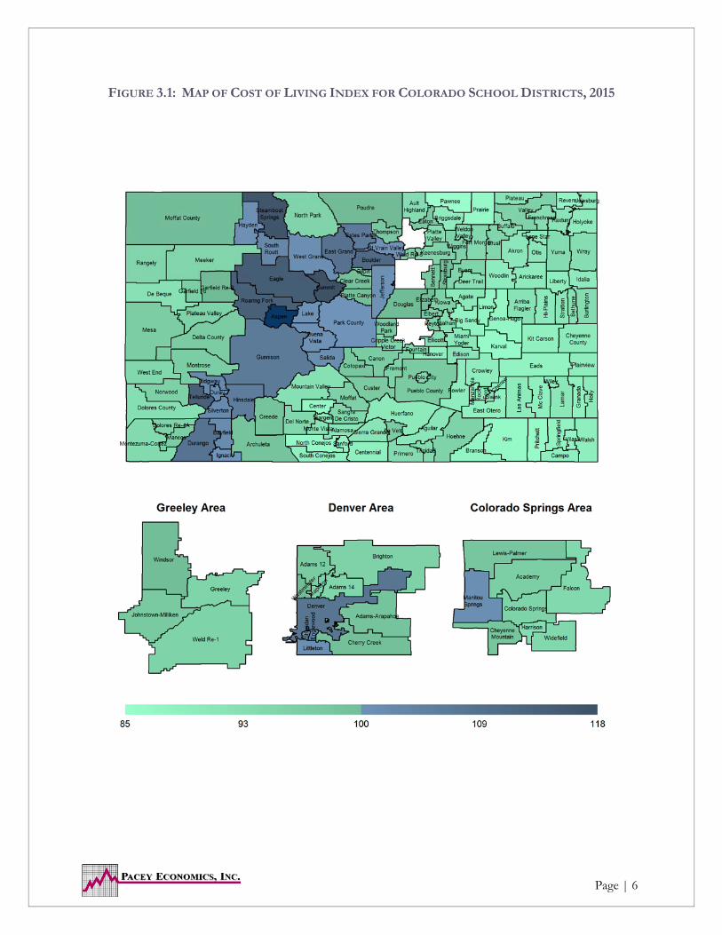
Figure 3.1, the state map following this discussion, provides a visual summary of the relative cost of living for each school district in the state of Colorado. Shades of green are below the indexed value of 100 and represent school districts that have annual expenditures below the average statewide Colorado teacher’s salary indexed at $51,900 with the lightest shades representing the lowest cost of living school districts and, as the green darkens, the annual average expenditures are moving toward the statewide average. Shades of blue are above the indexed value of 100 and identify school districts with higher than the statewide average salary with the lighter blue noting at or near the statewide average and the darkest blue identifying the school districts with the highest cost of living. This ranking is relative to all 178 school districts within the state utilizing the average statewide Colorado teacher’s salary income (for teachers with a Bachelor’s degree and 10 years or more of experience) of $51,900 for the “benchmark” household. (Importantly, school districts have varying salary schedules and the data indicate higher cost of living school districts tend to have higher average salaries and the lower cost of living school districts tend to have similarly lower average teacher salaries.)

Figure 3.1 also isolates some of the more populated Front Range area school districts for visual clarity of their relative rankings for cost of living. Following the mapping of school district rankings, Table 3.1, which extends across several pages, identifies the average annual expenditures for the “archetypical” household and notes, in alphabetical order by county, both the school district’s average annual expenditures as well as their ranking in the 2015 study. (These findings are also delineated by rank in Appendix A.)

Although the 2015 study incorporates some improved methodological changes, a key “change” in the 2015 study was the measurement of household income. In past studies household income was considered to be the average Colorado teacher’s salary while the 2015 measurement considers the average Colorado teacher’s salary with a Bachelor’s degree and ten or more years of experience. In previous studies the trend of the average Colorado teacher’s salary increased consistent with expected wage growth; however, over the 2011 to 2015 period income for this metric was either flat or decreasing. Additional research suggested this decrease appeared to be related to a greater rate of exit of higher paid teachers (either through retirement or alternative employment opportunities) with a concomitant greater increase in entry-level teaching positions at the expected lower entry-level wages, serving to lower the statewide average teacher’s salary. This phenomenon is consistent with demographic changes (Baby Boomers retiring, a reviving economy since 2008, etc.) while in earlier years the rate of entry/exit was likely more evenly distributed. Given this phenomenon, the Colorado Legislative Council determined, and Pacey Economics, Inc. concurred, the use of the average Colorado teacher’s salary with a Bachelor’s degree and 10 or more years of service was more representative of “typical” household income (and most likely representative of the average teacher profile utilized in earlier cost of living studies).

Page | 5 Page | 5

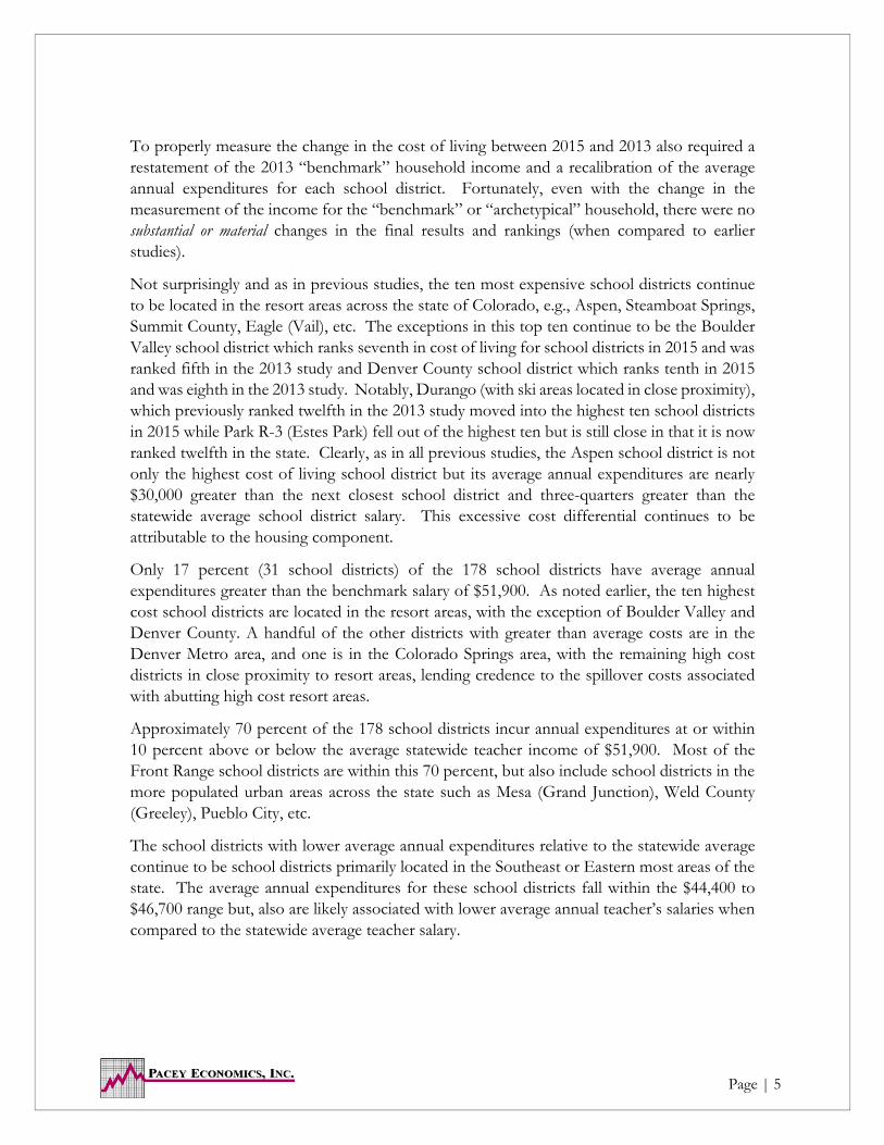
To properly measure the change in the cost of living between 2015 and 2013 also required a restatement of the 2013 “benchmark” household income and a recalibration of the average annual expenditures for each school district. Fortunately, even with the change in the measurement of the income for the “benchmark” or “archetypical” household, there were no substantial or material changes in the final results and rankings (when compared to earlier studies).

Not surprisingly and as in previous studies, the ten most expensive school districts continue to be located in the resort areas across the state of Colorado, e.g., Aspen, Steamboat Springs, Summit County, Eagle (Vail), etc. The exceptions in this top ten continue to be the Boulder Valley school district which ranks seventh in cost of living for school districts in 2015 and was ranked fifth in the 2013 study and Denver County school district which ranks tenth in 2015 and was eighth in the 2013 study. Notably, Durango (with ski areas located in close proximity), which previously ranked twelfth in the 2013 study moved into the highest ten school districts in 2015 while Park R-3 (Estes Park) fell out of the highest ten but is still close in that it is now ranked twelfth in the state. Clearly, as in all previous studies, the Aspen school district is not only the highest cost of living school district but its average annual expenditures are nearly $30,000 greater than the next closest school district and three-quarters greater than the statewide average school district salary. This excessive cost differential continues to be attributable to the housing component.

Only 17 percent (31 school districts) of the 178 school districts have average annual expenditures greater than the benchmark salary of $51,900. As noted earlier, the ten highest cost school districts are located in the resort areas, with the exception of Boulder Valley and Denver County. A handful of the other districts with greater than average costs are in the Denver Metro area, and one is in the Colorado Springs area, with the remaining high cost districts in close proximity to resort areas, lending credence to the spillover costs associated with abutting high cost resort areas.

Approximately 70 percent of the 178 school districts incur annual expenditures at or within 10 percent above or below the average statewide teacher income of $51,900. Most of the Front Range school districts are within this 70 percent, but also include school districts in the more populated urban areas across the state such as Mesa (Grand Junction), Weld County (Greeley), Pueblo City, etc.

The school districts with lower average annual expenditures relative to the statewide average continue to be school districts primarily located in the Southeast or Eastern most areas of the state. The average annual expenditures for these school districts fall within the $44,400 to $46,700 range but, also are likely associated with lower average annual teacher’s salaries when compared to the statewide average teacher salary.

Page | 6 Page | 6

FIGURE 3.1: MAP OF COST OF LIVING INDEX FOR COLORADO SCHOOL DISTRICTS, 2015

Page | 7 Page | 7

TABLE 3.1: 2015 COST OF LIVING INDEX FOR COLORADO SCHOOL DISTRICTS

School District ID

County School District Total Index Rank2015

State Average $51,930 100

10 Adams MAPLETON 1 49,261 94.9 75

20 Adams ADAMS 12 FIVE STAR SCHOOLS 50,059 96 56

30 Adams ADAMS COUNTY 14 48,972 94.3 88

40 Adams BRIGHTON 27J 49,271 94.9 74

50 Adams BENNETT 29J 50,405 97.1 50

60 Adams STRASBURG 31J 51,563 99.3 38

70 Adams WESTMINSTER 50 51,689 100 36

100 Alamosa ALAMOSA RE-11J 47,326 91.1 121

110 Alamosa SANGRE DE CRISTO RE-22J 48,807 94.0 91

120 Arapahoe ENGLEWOOD 1 54,315 104.6 14

123 Arapahoe SHERIDAN 2 52,115 100.4 30

130 Arapahoe CHERRY CREEK 5 51,342 98.9 41

140 Arapahoe LITTLETON 6 52,736 101.6 23

170 Arapahoe DEER TRAIL 26J 47,687 91.8 114

180 Arapahoe ADAMS-ARAPAHOE 28J 50,834 97.9 44

190 Arapahoe BYERS 32J 48,931 94.2 89

220 Archuleta ARCHULETA COUNTY 50 JT 50,802 97.8 45

230 Baca WALSH RE-1 46,134 88.8 153

240 Baca PRITCHETT RE-3 44,962 87 175

250 Baca SPRINGFIELD RE-4 45,663 87.9 163

260 Baca VILAS RE-5 45,535 87.7 167

270 Baca CAMPO RE-6 46,023 88.6 155

290 Bent LAS ANIMAS RE-1 46,420 89.4 146

310 Bent MC CLAVE RE-2 46,002 89 156

470 Boulder ST VRAIN VALLEY RE 1J 52,271 100.7 28

480 Boulder BOULDER VALLEY RE 2 57,880 111.5 7

490 Chaffee BUENA VISTA R-31 52,454 101.0 26

500 Chaffee SALIDA R-32 53,044 102.1 20

510 Cheyenne KIT CARSON R-1 45,863 88.3 161

520 Cheyenne CHEYENNE COUNTY RE-5 46,572 89.7 141

540 Clear Creek CLEAR CREEK RE-1 51,333 98.9 42

550 Conejos NORTH CONEJOS RE-1J 45,039 86.7 173

560 Conejos SANFORD 6J 45,570 87.8 166

580 Conejos SOUTH CONEJOS RE-10 46,048 88.7 154

640 Costilla CENTENNIAL R-1 45,993 89 157

740 Costilla SIERRA GRANDE R-30 47,258 91.0 125

Page | 8 Page | 8

TABLE 3.1: 2015 COST OF LIVING INDEX FOR COLORADO SCHOOL DISTRICTS (CONT’D)

1Fremont RE-2 was previously identified as Florence RE-2 in the 2013 study.

School District ID



770 Crowley CROWLEY COUNTY RE-1-J 46,365 89.3 147

860 Custer CUSTER COUNTY SCHOOL DISTRICT C-1 50,216 96.7 54

870 Delta DELTA COUNTY 50(J) 49,949 96.2 58

880 Denver DENVER COUNTY 1 56,456 108.7 10

890 Dolores DOLORES COUNTY RE NO.2 47,885 92.2 112

900 Douglas DOUGLAS COUNTY RE 1 51,773 99.7 34

910 Eagle EAGLE COUNTY RE 50 59,755 115 4

920 Elbert ELIZABETH C-1 51,702 99.6 35

930 Elbert KIOWA C-2 49,418 95.2 70

940 Elbert BIG SANDY 100J 45,647 87.9 164

950 Elbert ELBERT 200 49,584 95.5 68

960 Elbert AGATE 300 46,829 90.2 132

970 El Paso CALHAN RJ-1 47,606 91.7 117

980 El Paso HARRISON 2 48,087 92.6 104

990 El Paso WIDEFIELD 3 48,611 93.6 93

1000 El Paso FOUNTAIN 8 48,415 93.2 98

1010 El Paso COLORADO SPRINGS 11 49,186 94.7 79

1020 El Paso CHEYENNE MOUNTAIN 12 50,594 97.4 47

1030 El Paso MANITOU SPRINGS 14 52,860 101.8 21

1040 El Paso ACADEMY 20 49,765 95.8 65

1050 El Paso ELLICOTT 22 47,909 92.3 110

1060 El Paso PEYTON 23 JT 49,632 95.6 67

1070 El Paso HANOVER 28 45,916 88.4 160

1080 El Paso LEWIS-PALMER 38 50,649 97.5 46

1110 El Paso FALCON 49 48,479 93.4 95

1120 El Paso EDISON 54 JT 47,282 91.0 123

1130 El Paso MIAMI/YODER 60 JT 46,866 90.2 131

1140 Fremont CANON CITY RE-1 49,940 96.2 59

1150 Fremont FREMONT RE-21 49,238 94.8 76

1160 Fremont COTOPAXI RE-3 50,473 97.2 48

1180 Garfield ROARING FORK RE-1 59,263 114.1 6

1195 Garfield GARFIELD RE-2 51,867 100 33

1220 Garfield GARFIELD 16 49,697 95.7 66

1330 Gilpin GILPIN COUNTY RE-1 49,806 95.9 63

1340 Grand WEST GRAND 1-JT. 52,751 101.6 22

Page | 9 Page | 9


School District ID



1350 Grand EAST GRAND 2 56,874 109.5 8

1360 Gunnison GUNNISON WATERSHED RE1J 55,732 107.3 11

1380 Hinsdale HINSDALE COUNTY RE 1 55,446 107 13

1390 Huerfano HUERFANO RE-1 46,694 89.9 135

1400 Huerfano LA VETA RE-2 49,973 96.2 57

1410 Jackson NORTH PARK R-1 49,128 94.6 81

1420 Jefferson JEFFERSON COUNTY R-1 52,476 101.1 25

1430 Kiowa EADS RE-1 45,687 88.0 162

1440 Kiowa PLAINVIEW RE-2 46,281 89.1 151

1450 Kit Carson ARRIBA-FLAGLER C-20 47,447 91.4 118

1460 Kit Carson HI-PLAINS R-23 46,659 89.8 136

1480 Kit Carson STRATTON R-4 47,180 90.9 126

1490 Kit Carson BETHUNE R-5 47,653 91.8 115

1500 Kit Carson BURLINGTON RE-6J 48,111 92.6 103

1510 Lake LAKE COUNTY R-1 52,411 100.9 27

1520 La Plata DURANGO 9-R 56,602 109.0 9

1530 La Plata BAYFIELD 10 JT-R 53,322 102.7 18

1540 La Plata IGNACIO 11 JT 51,993 100.1 31

1550 Larimer POUDRE R-1 51,885 99.9 32

1560 Larimer THOMPSON R-2J 50,282 96.8 52

1570 Larimer PARK (ESTES PARK) R-3 55,496 107 12

1580 Las Animas TRINIDAD 1 48,335 93.1 100

1590 Las Animas PRIMERO REORGANIZED 2 48,309 93.0 101

1600 Las Animas HOEHNE REORGANIZED 3 49,183 94.7 80

1620 Las Animas AGUILAR REORGANIZED 6 47,108 90.7 127

1750 Las Animas BRANSON REORGANIZED 82 45,507 87.6 168

1760 Las Animas KIM REORGANIZED 88 45,020 86.7 174

1780 Lincoln GENOA-HUGO C113 45,295 87.2 171

1790 Lincoln LIMON RE-4J 45,498 87.6 170

1810 Lincoln KARVAL RE-23 44,858 86.4 177

1828 Logan VALLEY RE-1 49,237 94.8 77

1850 Logan FRENCHMAN RE-3 47,902 92.2 111

1860 Logan BUFFALO RE-4 47,956 92.3 108

1870 Logan PLATEAU RE-5 47,377 91.2 119

1980 Mesa DE BEQUE 49JT 47,615 91.7 116

1990 Mesa PLATEAU VALLEY 50 49,310 95.0 72

Page | 10 Page | 10


School District ID



2000 Mesa MESA COUNTY VALLEY 51 49,794 95.9 64

2010 Mineral CREEDE CONSOLIDATED 1 50,852 97.9 43

2020 Moffat MOFFAT COUNTY RE:NO 1 51,630 99.4 37

2035 Montezuma MONTEZUMA-CORTEZ RE-1 48,384 93.2 99

2055 Montezuma DOLORES RE-4A 49,124 94.6 82

2070 Montezuma MANCOS RE-6 49,841 96.0 62

2180 Montrose MONTROSE COUNTY RE-1J 49,870 96.0 60

2190 Montrose WEST END RE-2 48,592 94 94

2395 Morgan BRUSH RE-2(J) 48,866 94.1 90

2405 Morgan FORT MORGAN RE-3 48,440 93 97

2505 Morgan WELDON VALLEY RE-20(J) 48,069 92.6 105

2515 Morgan WIGGINS RE-50(J) 49,287 94.9 73

2520 Otero EAST OTERO R-1 45,968 89 158

2530 Otero ROCKY FORD R-2 46,562 89.7 142

2535 Otero MANZANOLA 3J 45,581 87.8 165

2540 Otero FOWLER R-4J 46,355 89.3 148

2560 Otero CHERAW 31 46,198 89.0 152

2570 Otero SWINK 33 47,262 91.0 124

2580 Ouray OURAY R-1 53,093 102.2 19

2590 Ouray RIDGWAY R-2 53,600 103.2 16

2600 Park PLATTE CANYON 1 51,491 99.2 40

2610 Park PARK COUNTY RE-2 52,153 100.4 29

2620 Phillips HOLYOKE RE-1J 46,605 89.7 138

2630 Phillips HAXTUN RE-2J 47,290 91.1 122

2640 Pitkin ASPEN 1 90,840 174.9 1

2650 Prowers GRANADA RE-1 45,947 88.5 159

2660 Prowers LAMAR RE-2 46,979 90.5 130

2670 Prowers HOLLY RE-3 46,597 89.7 140

2680 Prowers WILEY RE-13 JT 46,480 90 144

2690 Pueblo PUEBLO CITY 60 48,479 93.4 96

2700 Pueblo PUEBLO COUNTY 70 50,172 96.6 55

2710 Rio Blanco MEEKER RE1 49,019 94.4 86

2720 Rio Blanco RANGELY RE-4 49,065 94.5 84

2730 Rio Grande DEL NORTE C-7 48,646 93.7 92

2740 Rio Grande MONTE VISTA C-8 47,329 91.1 120

2750 Rio Grande SARGENT RE-33J 46,611 89.8 137

Page | 11 Page | 11


1Revere School District was previously identified as Platte Valley Re-3 in the 2013 study.

School District ID



2760 Routt HAYDEN RE-1 52,622 101.3 24

2770 Routt STEAMBOAT SPRINGS RE-2 60,901 117.3 3

2780 Routt SOUTH ROUTT RE 3 53,799 103.6 15

2790 Saguache MOUNTAIN VALLEY RE 1 47,761 92.0 113

2800 Saguache MOFFAT 2 49,449 95.2 69

2810 Saguache CENTER 26 JT 45,244 87.1 172

2820 San Juan SILVERTON 1 53,461 102.9 17

2830 San Miguel TELLURIDE R-1 59,275 114.1 5

2840 San Miguel NORWOOD R-2J 49,415 95.2 71

2862 Sedgwick JULESBURG RE-1 46,505 90 143

2865 Sedgwick REVERE SCHOOL DISTRICT1 45,502 87.6 169

3000 Summit SUMMIT RE-1 61,485 118.4 2

3010 Teller CRIPPLE CREEK-VICTOR RE-1 48,981 94.3 87

3020 Teller WOODLAND PARK RE-2 50,434 97.1 49

3030 Washington AKRON R-1 47,016 90.5 129

3040 Washington ARICKAREE R-2 46,714 90.0 134

3050 Washington OTIS R-3 47,021 91 128

3060 Washington LONE STAR 101 46,824 90.2 133

3070 Washington WOODLIN R-104 46,321 89.2 149

3080 Weld WELD COUNTY RE-1 49,206 94.8 78

3085 Weld EATON RE-2 50,252 97 53

3090 Weld KEENESBURG RE-3(J) 49,116 94.6 83

3100 Weld WINDSOR RE-4 51,507 99.2 39

3110 Weld JOHNSTOWN-MILLIKEN RE-5J 50,312 96.9 51

3120 Weld GREELEY 6 49,059 94.5 85

3130 Weld PLATTE VALLEY RE-7 48,178 92.8 102

3140 Weld WELD COUNTY S/D RE-8 49,846 96 61

3145 Weld AULT-HIGHLAND RE-9 48,026 92 106

3146 Weld BRIGGSDALE RE-10 46,431 89.4 145

3147 Weld PRAIRIE RE-11 44,880 86.4 176

3148 Weld PAWNEE RE-12 44,350 85.4 178

3200 Yuma YUMA 1 48,012 92.5 107

3210 Yuma WRAY RD-2 47,924 92.3 109

3220 Yuma IDALIA RJ-3 46,599 89.7 139

3230 Yuma LIBERTY J-4 46,295 89.1 150

Page | 12 Page | 12

SECTION 4: METHODOLOGY

4.1 IDENTIFYING THE “BENCHMARK” HOUSEHOLD

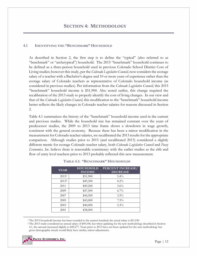
As described in Section 2, the first step is to define the “typical” (also referred to as “benchmark” or “archetypical”) household. The 2015 “benchmark” household continues to be defined as a three-person household used in previous Colorado School District Cost of Living studies; however this study, per the Colorado Legislative Council, now considers the average salary of a teacher with a Bachelor’s degree and 10 or more years of experience rather than the average salary of Colorado teachers as representative of Colorado household income (as considered in previous studies). Per information from the Colorado Legislative Council, this 2015 “benchmark” household income is $51,900. Also noted earlier, this change required the recalibration of the 2013 study to properly identify the cost of living changes. In our view and that of the Colorado Legislative Council, this modification to the “benchmark” household income better reflects the likely changes in Colorado teacher salaries for reasons discussed in Section 2.

Table 4.1 summarizes the history of the “benchmark” household income used in the current and previous studies. While the household size has remained constant over the years of predecessor studies, the 2009 to 2013 time frame shows a slowdown in wage growth, consistent with the general economy. Because there has been a minor modification in the measurement for Colorado teacher salaries, we recalibrated the 2013 results for the appropriate comparison. Although studies prior to 2015 (and recalibrated 2013) considered a slightly different metric for average Colorado teacher salary, both Colorado Legislative Council and Pacey Economics, Inc. believe there is reasonable consistency with the earlier studies as the ebb and flow of entry level teachers prior to 2013 probably reflected this new measurement.

TABLE 4.1: “BENCHMARK” HOUSEHOLDS

1 The 2015 household income has been rounded to the nearest hundred; the actual salary is $51,930. 2 The 2013 study considered an annual salary of $49,100, but when updating for the new methodology described in Section 4.1, the amount increased slightly to $49,277. Years prior to 2013 have not been updated for the new methodology but given demographic trends would likely have similar, minor adjustments.

YEAR HOUSEHOLD

INCOME PERCENT INCREASE/

DECREASE 20151 $51,900 5.4%

20132 $49,300 0.2%

2011 $49,200 3.6%

2009 $47,500 6.7%

2007 $44,500 3.5%

2005 $43,000 7.5%

2003 $40,000 5.3%

2001 $38,000

Page | 13 Page | 13

4.2 IDENTIFYING THE MARKET BASKET OF GOODS AND SERVICES

The 2015 study, as with all the cost of living studies since its inception in 1994, utilized the Consumer Expenditure Surveys (CES) conducted by the Bureau of Labor Statistics (BLS) to identify the probable expenditures for the “archetypical” household. Consumer/household spending habits have been tracked and quantified by the BLS in their annual CES for multiple decades. The CES identifies average annual expenditures for fourteen major expenditure categories, across nine income brackets for family sizes ranging from single persons to as many as five-person families, as well as several additional criteria not considered in this study. Within each of these major categories the CES data include dozens of specific items, measuring the average annual expenditure for each item and also determining the relative value (i.e., in percent) for each item to overall expenditures, given the composition and income level for the family.

The categories included in the “market basket” of goods and services represent the significant components of the “typical” or “benchmark” household’s spending habits for a three-person household with $51,900 of household income. Within each category, a list of goods and services was jointly compiled by the Colorado Legislative Council and Pacey Economics, Inc. to represent each major category of expenditure for this “archetypical” household. As in previous studies, the 2015 study considers the items selected for sampling to be:

a major percentage of the expenditure category;

sufficiently homogeneous to allow for price comparisons; and

a product (good) or service that is widely available throughout the state.

The specific items selected for price collection in the 2015 study include essentially the same goods and services as incorporated in the 2013 study but also added a few new products and replaced a few items. Table 4.2 on the following pages identifies the specific items surveyed in the 2015 study while changes to items previously included in the “market basket” are noted in the discussion following Table 4.2.

Page | 14 Page | 14

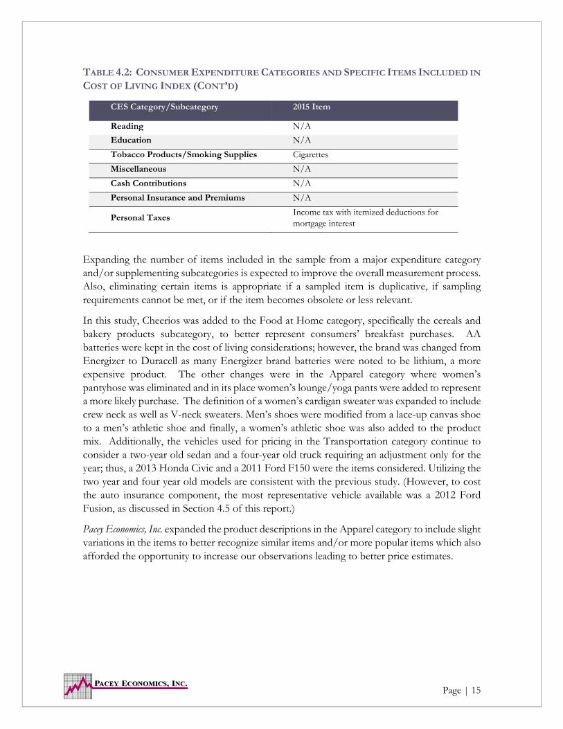
TABLE 4.2: CONSUMER EXPENDITURE CATEGORIES AND SPECIFIC ITEMS INCLUDED IN

COST OF LIVING INDEX

CES Category/Subcategory 2015 Item

Food at Home Cereals and bakery products White bread, spaghetti, Cheerios Meats, poultry, fish and eggs Ground beef, whole fryer chicken Dairy products Milk

Fruits and vegetables Bananas, potatoes, canned peaches, canned green beans

Other food at home Coffee, soup, frozen waffles

Food Away from Home Cheeseburger meal, cheese pizza meal, steak meal

Alcoholic Beverages BeerHousing

Shelter Mortgage payment/property taxes, homeowner’s insurance

Utilities Electric, natural gas, telephone, water/wastewater

Household operations Day care services Housekeeping supplies Laundry soap Household furnishings and equipment RefrigeratorApparel Men and boys Men’s dress shirt, men’s t-shirt

Women and girls Women’s cardigan sweater, women’s lounge/yoga pants

Footwear Men’s athletic shoes, women’s athletic shoes Transportation Vehicle purchases (net outlay) Car payment/auto financing Gasoline and motor oil 85 unleaded gasoline

Other vehicle expenses Vehicle finance charges (interest rate, bank financing fees), oil change, front end alignment, insurance premiums

Healthcare Health insurance premiumEntertainment Fees and admissions Movie ticket (first run, full length) Audio and visual equipment and

services Television

Pets, toys, hobbies, and playground equipment

Pet food

Other entertainment supplies, equipment, and services

AA batteries

Personal Care Products and Services Women’s haircut, men’s haircut, toothpaste, feminine hygiene product, shaving cream

Page | 15 Page | 15

TABLE 4.2: CONSUMER EXPENDITURE CATEGORIES AND SPECIFIC ITEMS INCLUDED IN

COST OF LIVING INDEX (CONT’D)

CES Category/Subcategory 2015 Item

Reading N/A

Education N/A

Tobacco Products/Smoking Supplies Cigarettes

Miscellaneous N/A

Cash Contributions N/A

Personal Insurance and Premiums N/A

Personal Taxes Income tax with itemized deductions for mortgage interest

Expanding the number of items included in the sample from a major expenditure category and/or supplementing subcategories is expected to improve the overall measurement process. Also, eliminating certain items is appropriate if a sampled item is duplicative, if sampling requirements cannot be met, or if the item becomes obsolete or less relevant.

In this study, Cheerios was added to the Food at Home category, specifically the cereals and bakery products subcategory, to better represent consumers’ breakfast purchases. AA batteries were kept in the cost of living considerations; however, the brand was changed from Energizer to Duracell as many Energizer brand batteries were noted to be lithium, a more expensive product. The other changes were in the Apparel category where women’s pantyhose was eliminated and in its place women’s lounge/yoga pants were added to represent a more likely purchase. The definition of a women’s cardigan sweater was expanded to include crew neck as well as V-neck sweaters. Men’s shoes were modified from a lace-up canvas shoe to a men’s athletic shoe and finally, a women’s athletic shoe was also added to the product mix. Additionally, the vehicles used for pricing in the Transportation category continue to consider a two-year old sedan and a four-year old truck requiring an adjustment only for the year; thus, a 2013 Honda Civic and a 2011 Ford F150 were the items considered. Utilizing the two year and four year old models are consistent with the previous study. (However, to cost the auto insurance component, the most representative vehicle available was a 2012 Ford Fusion, as discussed in Section 4.5 of this report.)

Pacey Economics, Inc. expanded the product descriptions in the Apparel category to include slight variations in the items to better recognize similar items and/or more popular items which also afforded the opportunity to increase our observations leading to better price estimates.

Page | 16 Page | 16

4.3 WEIGHTING THE MARKET BASKET OF GOODS AND SERVICES

Each item in the market basket must be weighted to reflect its cost relative to the annual expenditures of the “benchmark” household. That is, specific expenditures (food, clothing, transportation, etc.) represent a different percent of household income and thus, must be weighted accordingly to properly determine average cost and average change in the cost of living.

Again, and as noted earlier, a careful evaluation of Western region vis-à-vis national data confirmed similar expenditure profiles, allowing the spending patterns of the Colorado “benchmark” household to continue to utilize the national expenditure profile as developed by the BLS from CES data. As the data for three-person households with average household income of $51,900 fall within two Consumer Expenditure Survey income levels expenditure estimates required an interpolation process between three-person household incomes of $40,000 to $49,999 and three-person household incomes of $50,000 to $69,999 (from CES Table 3433). This weighted average most appropriately reflects the probable spending habits of the “benchmark” family with an annual income of $51,900. See Appendix G for the most recent and relevant Consumer Expenditure Survey table.

Table 4.3A on the following page shows the relative weights for the major expenditure categories sampled in this study based on data obtained from the 2013-2014 Consumer Expenditure Survey (Table 3433) for three-person households. Table 4.3A also compares the percentage of annual expenditures by category relative to overall expenditures since the 2003 study, a dozen years ago. Not surprisingly, the largest three consumer expenditure categories in the 2015 study continue to be Housing, Transportation, and Food, making up over 60% of consumer expenditures in 2015 but over 65% in 2003. This decrease of overall expenditures for basic food, shelter and transportation allows for some additional income to be available for other goods and services.

Page | 17 Page | 17

TABLE 4.3A: SPECIFIC MAJOR CATEGORY EXPENDITURE WEIGHTS UTILIZED IN

MEASURING COST OF LIVING – (WEIGHT AS A PERCENTAGE OF INCOME)

Expenditure Category % of Income

2015

% of Income

2003

Food 13.67% 13.83%

Alcoholic Beverages 0.60% 0.70%

Housing 31.55% 28.80%

Apparel 3.21% 4.77%

Transportation 17.72% 22.51%

Healthcare 7.74% 5.13%

Entertainment 4.72% 4.72%

Personal Care Products and Services 1.13% 1.40%

Tobacco 0.87% 1.08%

Personal Taxes 5.12% 3.43%

Other 13.66% 13.62%

Total* 100% 100%

*Total does not sum to exactly 100% due to rounding.

The largest changes in the weight of expenditures over the last dozen years were primarily noted in the transportation, housing, and healthcare categories. Transportation expenditures decreased nearly 5 percentage points (more than a 20 percent decrease) and likely represents decreased costs associated with technological innovations and lifestyle trends including more efficient transportation, increase in urban living, etc. Housing expenditures increased by 2.75 percentage points or nearly 10 percent (28.8% to 31.55% of household income over the twelve year period). This increase is most likely associated with long term home price appreciation and a concomitant increase in property taxes as well as an increase in utility consumption as rates and usage increase. On the other hand, although not separately identified in Table 4.3A, the proportion of housing expenditures for mortgage interest and charges have decreased over the past dozen years as interest rates have remained at historical lows. The healthcare expenditure increase since 2003 of just over 2.5 percentage points (or over 50%) reflects increases in health insurance as well as data noting medical goods and services continue to outpace the inflation rate in nonmedical goods and services.

Table 4.3B provides a more detailed weighting of each category and subcategory and its respective item(s) considered in the “market basket” of goods and services purchased by the “benchmark” household for 2015 compared to the previous cost of living study in 2013.

Page | 18 Page | 18

TABLE 4.3B: SPECIFIC MAJOR AND SUB-CATEGORY EXPENDITURE WEIGHTS UTILIZED

IN MEASURING THE COST OF LIVING – (WEIGHT AS A PERCENTAGE OF INCOME)

Expenditure Category % of

Income 2015

% of Income

2013

2015 Representative Market Basket Items

Food 13.67% 13.59%

Food at home 8.61% 8.51%

Cereals and bakery products 1.18% 1.26%

Cereals and cereal products 0.41% 0.45% Cheerios

Bakery products 0.77% 0.81% white bread, spaghetti

Meats, poultry, fish, and eggs 1.86% 1.92%

Beef 1.11% 1.22% ground beef

Poultry 0.75% 0.69% whole fryer chicken

Dairy products 0.90% 0.90% milk

Fruits and vegetables 1.52% 1.43%

Fresh fruits 0.52% 0.50% bananas

Fresh vegetables 0.47% 0.43% potatoes

Processed fruits 0.24% 0.23% canned peaches

Processed vegetables 0.29% 0.26% canned green beans

Other food at home 3.14% 3.01% coffee, soup, frozen waffles

Food away from home 5.06% 5.08% cheeseburger meal, cheese pizza meal, steak meal

Alcoholic Beverages 0.60% 0.65% beer

Housing 31.55% 33.77%

Shelter 17.32% 18.45%

Mortgage interest and charges

12.98% 14.06% mortgage payment

Property taxes 2.72% 2.83% property taxes

Maintenance, repairs, insurance, other expenses

1.62% 1.56% homeowner’s insurance

Utilities, fuels, and public services

8.46% 8.68%

Natural gas 0.85% 0.88% natural gas

Electricity 3.37% 3.51% electric

Telephone services 3.20% 3.19% telephone

Water and other public services

1.04% 1.11% water, wastewater

Household operations 2.05% 2.44% day care services

Housekeeping supplies 1.15% 1.37% laundry soap

Household furnishings and equipment

2.57% 2.83% refrigerator

Apparel 3.21% 3.30%

Men and boys 0.83% 0.77% men’s dress shirt, men’s t-shirt

Women and girls 1.48% 1.56% women’s cardigan sweater, women’s lounge/yoga pants

Footwear 0.90% 0.96% men’s athletic shoes, women’s athletic shoes

Page | 19 Page | 19

TABLE 4.3B: SPECIFIC MAJOR AND SUB-CATEGORY EXPENDITURE WEIGHTS UTILIZED

IN MEASURING THE COST OF LIVING – (WEIGHT AS A PERCENTAGE OF INCOME)

(CONT’D)

1 The marked increase in personal taxes in 2015 from the 2013 study is due to the CES including imputed values in 2015. *Total does not sum to exactly 100% due to rounding.

Expenditure Category % of

Income 2015

% of Income

2013

2015 Representative Market Basket Items

Transportation 17.72% 19.25%

Vehicle purchases (net outlay) 6.74% 7.05% car payment/auto financing

Gasoline and motor oil 6.14% 7.00% 85 unleaded gasoline

Other vehicle expenses 4.84% 5.70%

Vehicle finance charges 0.61% 0.59% interest rate, bank financing fees

Maintenance and repairs 1.75% 1.90% oil change, front end alignment

Vehicle insurance 2.47% 3.31% insurance premiums

Healthcare 7.74% 7.34% health insurance premiums

Entertainment 4.72% 4.45%

Fees and admissions 0.71% 0.77% movie ticket

Audio and visual equipment and services

2.06% 2.06% television


1.11% 1.05% pet food


0.84% 0.56% AA batteries

Personal Care Products and Services

1.13% 1.11% women’s haircut, men’s haircut, toothpaste, tampons, shaving cream

Reading 0.12% 0.15%

Education 1.54% 1.91%

Tobacco Products and Smoking Supplies

0.87% 1.22% cigarettes

Miscellaneous 1.75% 1.45%

Cash Contributions 2.15% 2.08%

Personal Insurance and Pensions

8.09% 8.23%

Personal Taxes1 5.12% 1.49% income tax with itemized deductions for mortgage interest

Total (bold level)* 100.00% 100.00%

Page | 20 Page | 20

Table 4.3A finds housing expenditures have only increased by some 2.75 percentage points over the last dozen years yet Table 4.3B notes a decrease in housing expenditures since 2013. Given further investigation of the subcomponents of the category, Pacey Economics, Inc. found the recent decrease to be associated with slightly lower average costs in mortgage payments and/or lower overall operating costs; however, the difference was small enough it may also simply be due to random sampling issues.

Of note, personal taxes saw a significant increase from 1.49% in 2013 to 5.12% in 2015; however, our research indicated this change was not due to tax increases but rather to changes in the BLS methodology for collecting personal tax information since 2013. [Over the past dozen years the methodology utilized by the BLS for determining personal taxes in the CES has undergone a number of revisions.] In the 2012 CES, the BLS survey asked respondents how much they paid in taxes and, for the 2014 CES, the estimated taxes came from a program developed by the National Bureau of Economic Research on actual income data which has nearly tripled the value of the 2012 survey responses. The new estimates are considered more accurate than the survey answers.

As in previous studies, there are miscellaneous subcategories within major expenditure categories which are not represented with specific items sampled. In order to maintain the total weights for the major expenditure categories the weights associated with the unrepresented subcategories, e.g., Children under age 2 in Apparel, were allocated to the other specifically sampled subcategories on a pro rata basis. As non-sampled subcategories comprise a small portion of the expenditure category, this methodology does not have a material impact on the measurement of the overall cost of living factors for each school district.

Finally, other major expenditure categories in the CES data for Reading, Education, Miscellaneous, Cash Contributions, and Personal Insurance and Pensions were not sampled but are expected to be constant for the relevant “archetypical” household. That is, given the nature of these categories, it was reasonable to expect no significant variation across the state for the “benchmark” household. (This methodology is consistent with the earlier cost of living studies, and, in our view, continues to be a reasonable assumption.)

Page | 21 Page | 21

4.4 DATA SOURCES AND COLLECTION PROCEDURES

Section 4.4 explains how the business establishments were determined in this analysis and outlines the data sources and collection procedures utilized, while Section 4.5 provides the detailed explanation of the data for each expenditure category. Section 4.6 describes the methodology considered to determine where the goods and services were purchased.

Measuring the 2015 price for each item in the representative basket of goods and services required identifying all the potential business establishments where households could choose to shop. Business establishment information was drawn primarily from Hoover’s, Inc. (a subsidiary of Dunn and Bradstreet) which identified approximately 400,000 Colorado businesses by various characteristics including industry, revenue and geography. Hoover’s, Inc. tracks establishments upon opening but not necessarily when or if they close and, not surprising, a number of stores in both urban and rural areas had closed. Consequently, to supplement the data, we instructed the field data collectors to survey a similar business establishment in the same area whenever possible if one of their designated stores had closed. This was particularly important in rural areas where sample sizes (i.e., the number of observations collected) were small. A combination of these sources provided the best estimate of the total population of vendors/business establishments for the state of Colorado. From these data sources, Pacey Economics, Inc. identified the list of vendors both by city and by major expenditure category to be sampled. The population of businesses were tracked to school districts by obtaining latitude and longitude coordinates for each business address from Texas A & M Geoservices which was then translated into school district shape files available from the U.S. Census Bureau.

Once all potential business establishments were identified, a sample size was determined. After researching efficient and effective sample sizes, a sample of 10 businesses per item per school district was determined to be the minimum target. Additionally, our data target was to collect at least as much data as in the 2013 study, even though additional businesses/observations may provide only limited gains in accuracy. To meet this goal, two modifications were made: 1) if there were five or fewer businesses in the sampling frame, Pacey Economics, Inc. included them all in the sample which was consistent with the previous contractor in the 2013 study, and 2) if our sample size was smaller than the number of observations in the 2013 study, Pacey Economics, Inc. increased our sample size to match at least the number of observations in the 2013 study. This methodology ensured that we target at least as much data as in the 2013 study, and that we make the most efficient use of the data in terms of the accuracy of the cost of living measure for each school district. A more detailed discussion of our sampling methodology and the changes from the previous study follows in Appendix B.

Once the sample size was determined (i.e., how many businesses in each school district to visit), the next step was to determine the sampling frame, i.e., the list of businesses from which the sample for a particular item is drawn. As the core source of business information was Hoover’s Inc. (a subsidiary of The Dun & Bradstreet Corporation), a subset of those businesses that are likely to carry that item was identified and used as the sampling frame for each item. Of note, convenience stores were included in the 2015 sample for several of the representative

Page | 22 Page | 22

goods, which is a change from the previous study. Convenience stores were included as consumers do typically purchase some items such as bread, feminine products, beer, etc. from these locations. However, other items (such as toothpaste and shaving cream) were not collected at convenience store sites as the items to be priced were not typically stocked in the specified sizes (e.g., 6.4 oz. toothpaste, 10 oz. shaving cream).

Given the sample size and the sampling frame, the final step was to draw a random sample. In a simple random sample, each business in the sampling frame has an equally likely chance of being selected. Randomness is important so that the sample properly reflects the underlying population, and so that statistical methods can be used to assess the accuracy of the price estimates and of the final cost of living measures. However, a somewhat more complex sampling method was used in this study to recognize that shoppers are more likely to purchase items from large stores than from small stores. In particular, the probability of a business being selected in a sample was proportional to the number of business employees, a proxy for business size. Of note, the 2013 study incorporated a similar sampling technique, with the probability of selection proportional to a store’s estimated revenues.

BUSINESS DISTRIBUTION

It is also no surprise that the number of businesses in each school district varies widely across the state. This variability is reflected below in Figure 4.4 which illustrates the geographic location of the grocery stores (e.g., King Soopers, Safeway, etc.) and Super Centers (e.g., Walmart, Target, Costco, etc.) by school district boundaries while Table 4.4 tabulates the number of grocery stores by the number of school districts.

FIGURE 4.4: GROCERY STORE LOCATIONS FOR COLORADO SCHOOL DISTRICTS, 2015

Page | 23 Page | 23

Of note, about one-quarter of the school districts in the state have no grocery stores, and another quarter only have one grocery store in their school district. Again, it is not surprising the school districts with limited shopping opportunities are in rural locations and likely require travel for many of their purchases, as vendors are not available within the geographical area. It has also been our experience that businesses in the rural locations tend to be more fluid (i.e., more frequent openings and closings of business establishments), with rural areas having a greater mismatch between the businesses actually operating, as identified by our data collection team, and those identified in in the Hoover’s, Inc. database.

TABLE 4.4: NUMBER OF SCHOOL DISTRICTS BY NUMBER OF GROCERY STORES

Number of Grocery Stores Number of School

Districts

0 47

1 46

2-4 38

5-9 17

10-24 14

25-49 6

50-99 7

100 or more 3

Total 178

AVENUES OF DATA COLLECTION

To obtain prices for the selected items in the “market basket” of goods and services, the following avenues for data collection were undertaken for the various market components:

ON-SITE DATA COLLECTION

Pacey Economics, Inc. retained temporary contract employees (paid hourly plus mileage and expenses) to perform the data collection in the field. Each contractor underwent a training session with a Pacey Economics, Inc. professional who had previously served as the field research manager when involved in past data collection projects.

Each field collector was provided a notebook containing store information, price sheets, pricing data required and product specifications, among other materials. On-site data collection was completed within a specified two week period (in early September 2015) and during that time frame cross-checks were also made randomly across stores. Data was recorded by hand at the time of collection and entered electronically at a later date and all price sheets were retained, serving as additional cross-checks on prices across school districts.

Page | 24 Page | 24

On-site visits were conducted for all items in the major expenditure categories of Food at Home, Food Away from Home (except for pizza), Alcoholic Beverages, Apparel and Services, Entertainment (except for movie tickets), Personal Care Products and Services (except men's and women's haircuts), Tobacco, as well as the representative item in Housekeeping Supplies (laundry soap) and Household Furnishings and Equipment (refrigerator) subcategories.

TELEPHONE CALLS DATA COLLECTION

Pacey Economics, Inc. personnel surveyed price information by telephone for oil changes, front-end alignments, men’s and women’s haircuts, vehicle financing rates and fees, and in some areas for pizza meals and movie tickets.

ONLINE DATA COLLECTION

Where possible and where available, Pacey Economics, Inc. personnel collected prices online for pizza meals and movie tickets. If information was not available online, prices were acquired by telephone.

Additionally, per responses in the shopping pattern survey, households sometimes purchased goods online. To account for online purchases, Walmart prices were used for goods purchased online, except for refrigerator prices, which were obtained from Lowe’s and Home Depot stores. These prices were held constant across the state of Colorado.

PUBLIC SOURCES

Pacey Economics, Inc. personnel also obtained prices as described in more detail in the following section from third party sources for the following items: day care, gasoline prices, mortgage payment/property taxes, homeowner’s insurance, vehicle insurance, health insurance, and utilities – electric, natural gas, water/wastewater, and telephone.

Each major expenditure category and/or subcategory is delineated in Section 4.5 and provides a more thorough explanation of the goods and services and the data collection process, and notes the exceptions or adjustments required to proceed with the final analysis.

Page | 25 Page | 25

4.5 DETAILED EXPLANATION OF DATA FOR EXPENDITURE CATEGORIES

For each expenditure item, applicable taxes were applied to the prices of the goods described below. Taxes include the Colorado state sales tax of 2.9% in addition to specific county, city, and/or special taxes (e.g., food/beverages for immediate consumption). Because taxes were collected on a city and county basis, taxes were allocated to the school districts on a pro rata basis and an average weighted tax was then determined using the shopping pattern survey. This methodology is explained in more detail in Section 4.6. Taxes were not applied to services as they are not a taxable good (as detailed in the sections below) and also took into account county- or municipality-specific exemptions for food at home, gas, electricity, etc.

FOOD

Food expenditures include not only food purchased for preparation in the home, but also food consumed outside of the home. This study represents both categories with the specifics detailed below.

FOOD - FOOD AT HOME

All food at home items were collected through on-site visits to stores throughout the state from the random sample of grocery outlets obtained from the Hoover’s, Inc. data set. This selection process included not only traditional grocery stores such as King Soopers, Safeway, etc., but also various discount retailers now selling food items such as Walmart and Target stores in addition to warehouse type outlets such as Costco and Sam’s Club. Oftentimes, especially in rural areas, a business enterprise had closed (as noted earlier, Hoover’s Inc. data collects business establishment data when applications for tax identification numbers are filed with the State but are not necessarily deleted from their files when a business closes). When the sample included a closed business in a particular city and/or if there were duplicates, wrong addresses, etc., then the list of stores to be sampled was supplemented with a similar store in the area as identified by the field collectors. This method of supplementing the Hoover’s, Inc. data was also used for all other categories in which on-site surveying was completed. Grocery tax was then added to each price in each location and an average price for each item was aggregated to the school district level by using the shopping pattern survey.

Page | 26 Page | 26

TABLE 4.5A: FOOD AT HOME

CES Category

Specific Item

Description Collection Method

Number (N) of Observations

Cereals and bakery products

White Bread

Price for store brand 24 oz. (1.5 lb.) loaf of sliced white bread. If store brand not available, record price of lowest priced brand with a 24 oz. loaf. Note any differences in brand or loaf size (Safeway store brand is 22 oz. - record this price and note difference).

On-site survey

577


Cheerios Price of General Mills Cheerios Toasted Whole Grain Oat Cereal plain, 12 oz. If size not available, note difference in size and record price.

On-site survey

569


Spaghetti Price of store brand spaghetti noodles, 16 oz. package. If store brand is not available, record price of lowest priced brand and note brand. Do not price premium store brands.

On-site survey

586

Dairy Milk Price for one gallon (128 fl. oz.) 2% milk, store brand. If no store brand, collect cheapest price and note. If no 2%, then price (in order of preference) 1%, skim, and whole. Note if not 2%. No organic, no soy, no flavored milks (e.g. chocolate, etc.). Do not price half gallon.

On-site survey

685

Fruits and vegetables

Bananas Price per pound. If bananas are priced by the bag or by the banana, report the price and weigh a bunch, note weight and number of bananas in bunch. Do not price organic.

On-site survey

380


Potatoes Price for a 10 lb. bag of lowest price Russet potatoes. If 10 lb. bag is not available, substitute nearest sack size and note size. If potatoes only sold individually, record price per pound and note. If sold individually, regardless of weight, record price and weigh potato. Do not use price of potatoes by the pound if sold in any size sack.

On-site survey

347


Canned Peaches

Price of store brand sliced peaches in heavy syrup, 15 to 15.25 oz. If no store brand, collect the cheapest brand and note brand.

On-site survey

531


Canned Green Beans

Price of store brand cut green beans, 14.5 oz. If no store brand, collect the cheapest brand and note brand.

On-site survey

632

Page | 27 Page | 27

TABLE 4.5A: FOOD AT HOME (CONT’D)

CES Category

Specific Item


Number (N)

of Observations

Other food at home

Coffee Price for an 11.3 oz. can of Folgers Classic Roast Coffee, ground, red can. If Folgers Classic Roast not available, price other ground Folgers in similar sizing (approx. 11 oz.). If not Folgers, price Maxwell House 11.5 oz. or nearest size. Note brand, product, and any size differences. Do not price decaffeinated or whole bean. Do not price any other brands.

On-site survey

632

Other food at home

Soup Price for a 10.75 oz. can of Campbell's Original Chicken Noodle Soup. If no Campbell's (rare), price store brand and note brand and any size difference. Do not price "HomeStyle" or "Classic" packaging or other variations.

On-site survey

676

Other food at home

Frozen Waffles

Price of store brand frozen waffles, buttermilk or plain flavored, prebaked, 10 pack, 12.3 oz. If store brand not available, record price of lowest priced brand and note brand and any differences in size. (Walmart store brand only has 8 pack - record price and note quantity.)

On-site survey

440

Meats, poultry, fish, and eggs

Whole Fryer Chicken

Price per pound of one whole fryer chicken, least expensive brand. If whole fryer chicken not available, price cut up whole fryer chicken and note.

On-site survey

332

Meats, poultry, fish, and eggs

Ground Beef

Price per pound of prepackaged, regular ground beef, 80% lean or most comparable, from a 1 to 2 pound package of loose ground beef. Note if different percent lean. Do not price family pack. Do not price pre-formed beef patties or tube packaging.

On-site survey

366

FOOD - FOOD AWAY FROM HOME

Food away from home included a cheeseburger meal, a pizza meal, and a steak meal as described in Table 4.5B. A standard cheese pizza was collected in the 2015 report instead of the more specific Pizza Hut cheese pizza used in the 2013 study. However, and not unexpectedly given the competitive pizza market, broadening the collection process to include a wider array of pizza stores did not alter the average price in any significant way.

The cheeseburger and steak meals were collected through on-site visits to dining establishments while the cheese pizza meal was predominantly collected online, but supplemented with telephone calls as necessary. The Hoover’s, Inc. data does not directly identify which restaurants served the particular items sampled (i.e., which restaurants served pizza, cheeseburgers, and/or steaks), so a preliminary classification was performed based on the store name (for example, a restaurant

Page | 28 Page | 28

was identified as likely to serve steak if the name contained “Applebee”, “Chili”, “Cafe”, “Inn”, etc.) Field surveyors supplemented the price data collection with additional establishments, when necessary.

Finally, the appropriate dining tax was added for each location and then the average prices for each item were aggregated to the school district level by using the shopping pattern survey.

TABLE 4.5B: FOOD AWAY FROM HOME

ALCOHOLIC BEVERAGES

Beer represents the Alcoholic beverage category and prices were collected at grocery stores, convenience stores as well as liquor stores. As with the other items, appropriate sales tax is added with average prices for each item aggregated to the school district level by using the shopping pattern survey.

CES Category

Specific Item



Food away from home

Cheeseburger Meal

Price for a McDonald's quarter pounder with cheese meal (including fries and a regular 21 oz. Coke). If not collecting at a McDonald's, price a cheeseburger with a medium fry and a Coke (the most similar type of meal to a quarter pounder with cheese meal).

On-site survey

805

Food away from home

Cheese Pizza Meal

Price for a cheese pizza, regular or thin crust, 14" diameter (note size if other).

Telephone survey & online sources

341

Food away from home

Steak Meal Price for a 12 oz. Ribeye steak and two sides (potato, vegetable, soup or salad). If only one side is included, then add a side (potato or vegetable) or side salad. Note differences. If 12 oz. not available, price Ribeye in different size (note size). If Ribeye not available, price a New York Strip. If New York Strip not available, price a Sirloin. Note size of steak if not 12 oz. (Price this item at Applebee’s and Chili’s, where available; price the 10 oz. sirloin at TGI Fridays.) Do not price chopped Sirloin. Note if different steak than Ribeye.

On-site survey

317

Page | 29 Page | 29

TABLE 4.5C: ALCOHOL

CES Category

Specific Item



Alcoholic beverages

Beer Price for a 6-pack of 12 oz. bottles of Corona Extra or Light beer, 3.2% alcohol by volume or higher if collected in a liquor store. If Corona not available, then price (in order of preference) Pacifico, Modelo, and Budweiser - all in 6-packs of 12 oz. bottles. Note brand. Do not price cans.

On-site survey

582

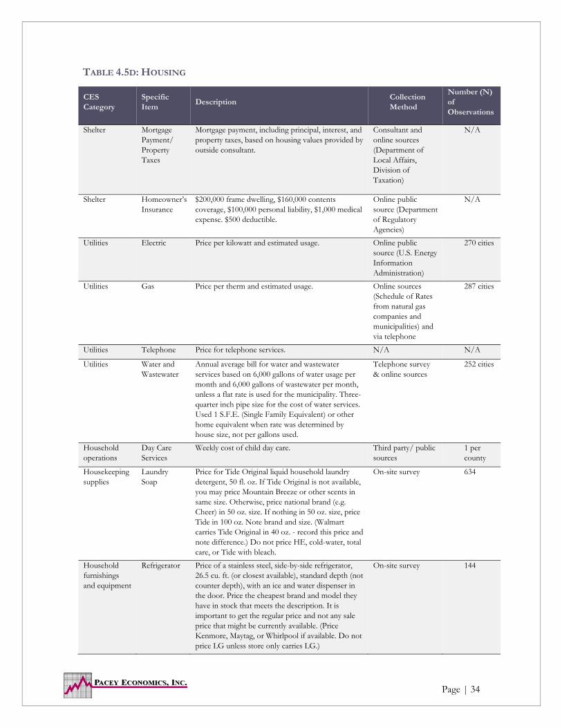
HOUSING

Expenditures on Housing, as noted below on Table 4.5D, include the categories for Shelter, Utilities, Household Operations and Supplies plus Household Furnishings and Equipment, with nearly 80% of housing costs attributable to Shelter and Utilities. In addition, Shelter has three subcomponents; mortgage payment in addition to property taxes and homeowner’s insurance, while Utilities considers four different subcomponents; electricity, gas, telephone, and water and wastewater expenditures. The subcomponents in each category are discussed below in more detail and then followed by a detailed discussion of the other components in the Housing category.

HOUSING - SHELTER

The Shelter subcategory estimated the cost of housing which included mortgage payments, property taxes and homeowner’s insurance. Pacey Economics, Inc. was responsible for adding in the cost of mortgage payments, based on housing value data for each school district provided by the Colorado Legislative Council through an outside consultant.

Mortgage payments were measured by Pacey Economics, Inc. by identifying the current 30-year fixed mortgage interest rate for Coloradans on December 28, 2015 and calculating a mortgage payment based on eighty percent of the home value, consistent with the methodology in previous cost of living studies.

Property tax estimates were then added based on the current assessment rate of 7.96%, obtained from the Final Analysis of the Estimated Residential Assessment for 2015-2016 from the Colorado Department of Local Affairs. The assessed value of the home was multiplied by the decimal equivalent of the total mill levy. The total mill levy was the sum of the mill levies from the county, city, school district, and any other special levies applicable in an area. (To calculate the decimal equivalent of a mill levy, the levy is multiplied by 0.001.)

Mill levies were obtained from the state of Colorado’s 2014 Forty-Fourth Annual Report to the Governor and the General Assembly produced by the Department of

Page | 30 Page | 30

Local Affairs, Division of Property Taxation and summed by school district. This is the value for the property tax subcomponent.

Homeowner’s insurance is another cost included under the Shelter category in the CES. Since the last study was completed, insurance companies have moved to more sophisticated cost platforms that require individualized information regarding credit rating, claim records, payment information, etc., preventing the continued use of the methodology used in previous studies for this component (i.e., to obtain individual quotes for each zip code from one insurance company using a hypothetical example). Fortunately, the Colorado Department of Regulatory Agencies now collects data for twenty-four cities in Colorado regarding homeowner’s insurance premiums from nearly 100 different insurance companies. The policy specifications are based on a home value of $200,000, contents replacement of $160,000, personal liability of $100,000, medical expense of $1,000 and a $500 deductible vis-à-vis previous study criteria of a $100,000 frame dwelling built in 1970 with $80,000 contents coverage, $100,000 liability/medical payments, and a $1,000 deductible. Although these specifications differ from the previous study, we found the adjustment and results were highly correlated to the 2013 study nor did such modification alter expected outcomes.

The methodology in the 2015 study utilized insurance premiums from the top 10 insurance companies in terms of market share (the top 10 companies accounted for over 60 percent of the total market share, and the remaining companies all had market shares of less than 2 percent). The insurance premiums for the top 10 companies in each of the twenty-four cities were used to predict premiums across the state using the spatial interpolation methodology (Kriging was the specific method used and Kriging is discussed in more detail in Appendix D to this report) for cities without data points. The individual city data were then aggregated to the school district level using the methodology described in Section 4.6 to obtain the final spending on insurance in each school district. Again, a detailed analysis/comparison of the current and previous data revealed relying on the Colorado Department of Regulatory Agencies data and the Kriging method (which incorporates data from 10 companies) rather than relying on information from only one company likely provides better price estimates for homeowner’s insurance.

HOUSING – UTILITIES

The subcategory referred to as Utilities, Fuels and Public Services represents the average annual bill for electricity, natural gas, telephone, and water and sewer services for each of the 178 school districts. The methodology used to compile these four expenditure subcategories is described below.

Electricity service price data utilized in this study were obtained from the U.S. Energy Information Administration which provided the electricity price per kilowatt for 270 cities in Colorado. Additionally, a portion of electricity costs were assumed

Page | 31 Page | 31

to vary with usage by tracking to cooling degree day data from National Oceanic and Atmospheric Administration (NOAA). That is, electricity costs in warmer climates were adjusted in accordance with the number of days that likely require air conditioning.

Our method differed from the 2013 methodology, in part as the data source utilized by the previous contractor was not available. However, our method likely better tracks usage patterns for different geographic areas (a limitation noted in the 2013 study). Moreover, using our method on the 2013 data found similar results, adding confidence to the efficacy of the 2015 methodology.

Once an average monthly electricity bill was calculated for each city the data were weighted and aggregated to each school district, and applicable taxes were applied. For school districts without price data, the Kriging methodology was utilized.

Natural gas service data was obtained from Services Rate Schedule from each of the five natural gas providers in Colorado which provided price data for 299 cities/townships. Additionally, six municipalities provide their own natural gas to their communities and these prices were collected online and via telephone. For school districts in which natural gas is not available, likely prices for propane were considered. Propane prices were estimated by first utilizing the Kriging methodology and then scaling natural gas prices in surrounding areas up by a factor of 1.72, the statewide differential cost of natural gas versus propane.

Similar to electricity, natural gas or propane usage was then estimated by utilizing heating degree days data (again, from NOAA) as natural gas usage varies quite directly with heating degree days.

The methodology used for obtaining natural gas prices is also a refinement from the previous study. Similar to the discussion above regarding electricity, we believe incorporating usage data yields somewhat superior results, especially as our natural gas pricing method on the 2013 data found similar results, again indicating confidence in the efficacy of the 2015 methodology.

Once an average monthly natural gas bill was calculated for each city the data were weighted and aggregated to each school district, and applicable taxes were applied.

Telephone deregulation within the industry and the ubiquity of cellular telephone use had led to essentially constant pricing across the state. As such, Pacey Economics, Inc. simply includes a constant cost of $128 per month where such an amount is consistent with the CES data which finds that 3.1% of household expenses were spent on telephone services. As with other taxable services, applicable taxes were incorporated.

Water and sewer service rates were calculated from information derived through online data collection and supplemented with a telephone survey of water and

Page | 32 Page | 32

sewer providers across the state of Colorado. Our survey resulted in over 250 water and sewer observations. Our survey was performed by Pacey Economics, Inc. personnel and data obtained on each provider’s particular charges includes flat fees, usage fees, drainage fees, base fees, etc.

The Geological Survey conducted by the U.S. Department of the Interior identifies “typical” household usage of 6,000 gallons of water per month. Thus, the average monthly water bill was calculated based on this level of water consumption and it is consistent with the previous study. The sewer bill was also calculated based on the 6,000 gallons of average usage in a month, and together these two components comprise the water/sewer bill. Once this total was calculated, applicable tax rates for each school district were incorporated.

Once an average monthly water and sewer bill was calculated for each city/municipality the data were weighted and aggregated to each school district, and applicable taxes were included. For cities where no price data was available or for cities/school districts that only use wells or septic tanks the Kriging methodology was applied.

HOUSING - HOUSEHOLD OPERATIONS

Day care costs incorporated in this study were based on information provided in The Self-Sufficiency Standard for Colorado 2015. This study was prepared for the Colorado Center on Law and Policy by the Center for Women’s Welfare at the University of Washington School of Social Work. Specific childcare costs for an infant (ages 0-1), a preschooler (ages 1-5), and a school-aged child (ages 5-13) were collected for each county in Colorado and then weighted by the proportion of children in care for each grouping, as reported by the Department of Health and Human Services data on children participating in Child Care and Development Fund (CCDF)-funded programs (Table 9 in their Fiscal Year 2014 publication).

The previous cost of living study obtained daycare costs from the 2013 Market Rate Survey of Child Care Providers, conducted by Qualistar; however, we were advised the Colorado Department of Human Services, Division of Child Care was no longer using Qualistar. We compared our data source, The Self-Sufficiency Standard for Colorado 2015 to the Child Care Affordability in Colorado Cost of Care Summary Report December 2014 authored by Qualistar and to the 2013 Market Rate Survey of Child Care Providers and found reasonably consistent costs for each of the age categories. The data used in this analysis matched very well to the 2013 data. Final average day care costs were aggregated from the county level to the school district level using the methodology described in Section 4.6.

For the purposes of the 2015 study, there was not specific delineation between childcare centers and family licensed providers as the data available now did not identify the type of provider. Notably, information suggests it is more likely that

Page | 33 Page | 33

family licensed providers will be prevalent in less populated, rural areas whereas childcare centers may be more prevalent in areas with higher populations and in the past, family licensed providers have been somewhat less expensive.

HOUSING - HOUSEKEEPING SUPPLIES

Laundry soap was the representative item sampled for the Housekeeping Supplies subcategory. Prices were collected at the same time and using the same methodology identified for food at home (grocery) items, i.e., on-site collection. Thus, for the most part, prices were collected at grocery stores, as well as general discount retailers such as Walmart and Target stores and/or Costco, etc.

Average laundry soap prices for each school district were obtained, sales tax was added, and aggregated using the results of the shopping pattern survey.

HOUSING - HOUSEHOLD FURNISHINGS AND EQUIPMENT

Refrigerator prices collected on-site at department stores, home stores, and electronic stores throughout the state were aggregated using the results of the shopping pattern survey. Sales tax was added to average refrigerator prices for each school district.

Page | 34 Page | 34

TABLE 4.5D: HOUSING

CES Category

Specific Item



Shelter Mortgage Payment/ Property Taxes

Mortgage payment, including principal, interest, and property taxes, based on housing values provided by outside consultant.

Consultant and online sources (Department of Local Affairs, Division of Taxation)

N/A

Shelter Homeowner’s Insurance

$200,000 frame dwelling, $160,000 contents coverage, $100,000 personal liability, $1,000 medical expense. $500 deductible.

Online public source (Department of Regulatory Agencies)

N/A

Utilities Electric Price per kilowatt and estimated usage. Online public source (U.S. Energy Information Administration)

270 cities

Utilities Gas Price per therm and estimated usage. Online sources (Schedule of Rates from natural gas companies and municipalities) and via telephone

287 cities

Utilities Telephone Price for telephone services. N/A N/A

Utilities Water and Wastewater

Annual average bill for water and wastewater services based on 6,000 gallons of water usage per month and 6,000 gallons of wastewater per month, unless a flat rate is used for the municipality. Three-quarter inch pipe size for the cost of water services. Used 1 S.F.E. (Single Family Equivalent) or other home equivalent when rate was determined by house size, not per gallons used.

Telephone survey & online sources

252 cities

Household operations

Day Care Services

Weekly cost of child day care. Third party/ public sources

1 per county

Housekeeping supplies

Laundry Soap

Price for Tide Original liquid household laundry detergent, 50 fl. oz. If Tide Original is not available, you may price Mountain Breeze or other scents in same size. Otherwise, price national brand (e.g. Cheer) in 50 oz. size. If nothing in 50 oz. size, price Tide in 100 oz. Note brand and size. (Walmart carries Tide Original in 40 oz. - record this price and note difference.) Do not price HE, cold-water, total care, or Tide with bleach.

On-site survey 634

Household furnishings and equipment

Refrigerator Price of a stainless steel, side-by-side refrigerator, 26.5 cu. ft. (or closest available), standard depth (not counter depth), with an ice and water dispenser in the door. Price the cheapest brand and model they have in stock that meets the description. It is important to get the regular price and not any sale price that might be currently available. (Price Kenmore, Maytag, or Whirlpool if available. Do not price LG unless store only carries LG.)

On-site survey 144

Page | 35 Page | 35

APPAREL

Our field data collectors obtained Apparel prices throughout the state. The items collected were men’s dress shirt, men’s t-shirt, women’s cardigan sweater, women’s lounge pants, and men’s and women’s athletic shoes. In the 2015 study, women’s pantyhose in the 2013 study was updated to women’s lounge/yoga pants, men’s canvas lace-up shoes were updated to men’s athletic shoes, and women’s athletic shoes were added. Business listings were identified from the Hoover’s, Inc. database but, again, supplemented by the field collectors when necessary.

Brands were specified for most apparel items; however, since not all stores have those specific brands, pictures of the items were included in the field surveyors’ packets so that they could find items which best resembled the stated items.

Once all data was collected, sales tax was added and an average price was calculated and aggregated to the school district level using the results of the shopping pattern survey.

TABLE 4.5E: APPAREL

CES Category

Specific Item



Men and boys

Men’s Dress Shirt

Price for white or solid color Oxford (button-down collar), long sleeve, button cuff shirt. Arrow brand where possible, poly/cotton blend. If store does not have Arrow, price comparable label that meets the same criteria. Try to get prices for shirts sized 15/32 through 16/34. Note size and brand.

On-site survey

283

Men and boys

Men’s T-Shirt

Price for one 3-pack of men's white t-shirts, V-neck. Hanes brand where possible, Fruit of the Loom or Jockey otherwise, 100% cotton. Must be in a 3-pack.

On-site survey

311

Women and girls

Women’s Cardigan Sweater

Price a women's solid color, long-sleeved V-neck (or crew neck), button front cardigan sweater, size M. 100% cotton or cotton/poly (or rayon/poly) blend. Price Old Navy Brand, where available; at Target, price Mossimo brand; at Walmart, price Bella Bird brand; at JC Penny's price Worthington brand; at Sears price Route 66. Note if other brand. Do not price cashmere or other wool.

On-site survey

337

Women and girls

Women’s Lounge/ Yoga Pants

Price a women's black wide leg or boot cut yoga pant/lounge pant/athletic pant, elastic band. Black legs may have print on top band. Medium size. (or sizes 4/6/8 - note if not M). Cheapest price, store brand (Mossimo for Target). Note brand and color if different from store brand and black. Cotton/polyester blend, jersey knit, cotton/spandex blend.

On-site survey

391

Footwear Men’s Athletic Shoes

Price a men's synthetic lace-up sneaker, rubber sole, size 9-11. Price the lowest priced men's athletic shoe that meets the described criteria. Minimal branding, note brand, and preferably solid black shoe. If not black, note color.

On-site survey

285

Page | 36 Page | 36

TABLE 4.5E: APPAREL (CONT’D)

CES Category

Specific Item



Footwear

Women’s Athletic Shoes

Price a women's synthetic lace-up sneaker, rubber sole, size 7-9. Price the lowest priced women's athletic shoe that meets the described criteria. Minimal branding, note brand, and preferably solid black or white shoe - if other color, note color.

On-site survey

287

TRANSPORTATION

Transportation is a critical component of everyday life as 17.72% of the “benchmark” family budget is allocated to this expenditure. In addition to a vehicle payment, transportation also consists of costs for vehicle insurance, oil and filter change and front end alignment (car maintenance and repair), and gasoline to recognize the full expenditures associated with the transportation needs of a family.

TRANSPORTATION – VEHICLE PAYMENTS

Vehicle payments were determined based on the purchase price of a 2013 Honda Civic LX Sedan, 4 door, 4-cylinder engine 1.8L, 5-speed manual transmission with 24,000 miles which was identified by using the Kelly Blue Book value of $14,500. (Of note, the 2013 study considered a 2011 Honda Civic as representative of a two-year old automobile.) The $14,500 was the base price used to calculate annual car payments. The actual purchase price was assumed to be constant throughout the state, consistent with previous cost of living studies. Financing rates and fees for a four year vehicle loan were obtained from telephone surveys of banking institutions and credit unions throughout the state. The list of banking institutions to survey came from information provided in the Hoover’s Inc. database.

Ownership taxes, registration and titling fees were obtained from Colorado Legislative Council Staff Issue Brief, “The Specific Ownership Tax”, the 2012 Colorado Motor Vehicle Law Resource Book, and verified on county websites and with the Colorado Revised Statutes. The vehicle weight is also required for calculating taxes which was obtained from the vehicle manufacturer’s website, American Honda Motor Company.

Average monthly car payments were then calculated, given the total amount financed (including the purchase price, all bank loan charges, and any applicable tax and registration fees) and the interest rate charged by the bank or credit union.

Page | 37 Page | 37

TRANSPORTATION – VEHICLE INSURANCE

Vehicle insurance premiums were obtained for 20 cities in the state from the Colorado Department of Regulatory Agencies. As with homeowner’s insurance, insurance companies have moved to more sophisticated cost platforms that require individualized information regarding credit rating, claim records, payment information, etc., preventing the continued use of the methodology used in previous studies for this component (i.e., to obtain individual quotes for each zip code from one insurance company using a hypothetical example). Fortunately, as with homeowner’s insurance, Pacey Economics, Inc. was able to identify insurance costs for a hypothetical driver with the following characteristics: a 35 year old male, married, principal operator, driving less than 15 miles to work each way, and has had no accidents or traffic violations in the past three years. The policy specifications also differed somewhat from the previous study and are now based on a driver of a 2012 Ford Fusion, the best representative automobile available to cost, with liability policy limits of $25,000/$50,000/$15,000, uninsured motorist coverage at $5,000 and a $500 deductible.

Similar to the methodology used for homeowner’s insurance, premiums for the top 10 auto insurers (which account for over 60 percent of the market share; with the remaining firms each having a market share of less than 2 percent) in each of the 20 cites was used to predict premiums across the state using spatial interpolation (i.e., Kriging, discussed earlier and also in Appendix D). The results were then aggregated to the school district level. Just as with homeowner’s insurance, results were compared to the 2013 study and this method was found to be effective, producing consistent and reliable results. Additionally, this methodology incorporated information from multiple firms as opposed to relying on information from a single firm.

TRANSPORTATION – MAINTENANCE AND REPAIRS

Maintenance and repairs included prices for front-end alignments and oil changes for the “benchmark” household’s 2011 Ford F-150 and were gathered through telephone surveys of various businesses throughout the state. Again, a randomly ordered list of the automobile service providers was generated from Hoover’s, Inc. The average prices for front-end alignments and oil changes were aggregated to the school district level by using the shopping pattern survey.

It should be noted that sales tax was only applied to parts for an oil change, and this was standardized across all oil change prices to reflect approximately 40 percent of the total oil change price. Therefore, 40 percent of all final oil change prices were taxed with the local sales tax, and the remaining 60 percent were left untaxed. Further, no tax was applied to front-end alignment prices because it is considered a service that is not taxed.

Page | 38 Page | 38

TRANSPORTATION – GASOLINE AND MOTOR OIL

Gasoline and motor oil expenditure considered unleaded grade 85 octane gasoline as the item to represent this category. Due to gasoline price fluctuations even over short periods of time, Pacey Economics, Inc. obtained the price for a gallon of gas on September 17, 2015 from every gasoline retailer in the state of Colorado using Oil Protection Information Services. This is an improved data collection procedure as the previous studies only took a sample of gas prices across the state. The average gas prices by city were then mapped into the appropriate school district and average school district prices were aggregated using the shopping pattern survey.

TABLE 4.5F: TRANSPORTATION

CES Category Specific Item



Transportation Vehicle Payment

Payment calculated for 2013 Honda Civic using Kelly Blue Book purchase value of $14,500 and interest rate on a four year loan with a good credit score (over 740, unless otherwise noted) for full purchase price, bank charges, taxes, and registration fees. Specifications for the 2013 Honda Civic LX Sedan include 4-doors, 4-cylinder engine, 1.8 Liter engine, 5-speed manual transmission, 24,000 miles on the vehicle, air conditioning, power steering, cruise control, and air bags.

Telephone survey

389

Transportation Vehicle Insurance

2012 Ford Fusion with liability policy limits of $25,000/$50,000/$15,000, $5,000 uninsured motorist coverage and with a $500 deductible.

Third party/ public source

N/A

Transportation Oil and Filter Change

Price of an oil and filter change for a 2011 Ford F150 pickup truck with a V6, 3.7 Liter engine. Oil must not be synthetic, filter should be the least expensive available. Do not price with tax. Mid-points used when ranges given.

Telephone survey

442

Transportation Front-End Alignment

Price of a front-end alignment for a 2011 Ford F150 pickup truck with 2-wheel drive. Mid-points used when ranges given.

Telephone survey

233

Transportation Gasoline 85 unleaded gasoline Third party 1728

HEALTHCARE

The healthcare insurance premiums were obtained from public information provided by the Colorado Division of Insurance which provides the actual rates for every participating health insurance company (more than 25) for a 40 year-old in each of the nine ‘rating areas’ in Colorado. The nine rating areas’ geographical boundaries track to metropolitan statistical areas

Page | 39 Page | 39

(MSAs) which do not overlap counties. Hence, the prices were first mapped to each county and then aggregated to the school district level to obtain the average rate for each school district. Notably, prices do not vary by gender (a requirement of the Affordable Care Act) and average price data for the most popular plans (“Bronze” and “Silver”) were considered. This methodology differs from that utilized in the previous study as, during the time between studies, the Affordable Care Act transformed the market by requiring insurance companies to have constant prices except by geography and age group.

TABLE 4.5G: HEALTHCARE

CES Category

Specific Item



Healthcare Health Insurance Premium

Prices of health care insurance premiums for a 40 year-old. Average price of “Bronze” and “Silver” health insurance premiums

Third party/ public sources

N/A

ENTERTAINMENT

Entertainment expenditures consisted of the subcategories fees and admissions, audio and visual equipment and services, pets, toys, and playground equipment, and other supplies with each detailed below.

ENTERTAINMENT - FEES AND ADMISSIONS

Movie prices were collected online, and when online data was not available, observations were supplemented with telephone calls for adult admission prices for weekend evening showings at the county level, given that many rural towns do not have a movie theater. For counties which did not have a movie theater, e.g., Washington County, the county data for the nearest location the family would likely travel to see a movie was applied. For instance, average movie price data for Logan County was also used to represent the average movie price for Washington County. The county averages for movie prices were then mapped to the appropriate school district.

ENTERTAINMENT - AUDIO AND VISUAL EQUIPMENT AND SERVICES

Television prices were sampled on-site across the state and then aggregated to the school district level based on the shopping pattern survey. Not surprisingly, many of the smaller (mostly rural) school districts often did not have electronics stores, and in those school districts field data collectors would do their best to find any store that sold televisions to obtain at least one price per school district. However, in several school districts, there were no television prices (due to a lack of stores selling televisions in that school district). For

Page | 40 Page | 40

school districts without a store selling a television, the shopping pattern survey was utilized to determine the relevant price. The applicable taxes were then included.

ENTERTAINMENT – PETS, TOYS, AND PLAYGROUND EQUIPMENT

Pet food prices were sampled on-site during the same September period other prices for goods and services were collected, mostly in larger retail stores and grocery stores, but also convenience stores. Taxes were added, and school district averages were then aggregated to the school district level based on the shopping pattern survey.

ENTERTAINMENT – OTHER SUPPLIES

Battery prices were sampled on-site at the same time grocery prices were collected. A change in the brand of the battery price collected was made as it was more readily available in grocery stores, discount stores, etc. Applicable taxes were added and school district prices were aggregated to the school district level based on the results of the shopping pattern survey.

TABLE 4.5H: ENTERTAINMENT

CES Category Specific Item



Fees and admission

Movie Price of adult admission to a first-run, full-length movie, weekend evening prices.

Telephone survey & online survey

70

Audio and visual equipment and services

Television Price of a 32" flat screen, LED TV: 720p, 60Hz HDTV. Samsung brand. If not available, LG brand, then Sony, then Panasonic. If exact options are not available, then priced 120Hz (32", LED, 720p). If not 32" then price next largest TV with same specs. Note brand and any differences in size or features. Do not price Plasma, LCD or 3D models.

On-site survey

164


Pet Food Price for a 5.5 oz. can of Friskies Classic cat food. If Friskies not available, price of 9Lives or Whiskas. Note brand and size. Do not price multipacks.

On-site survey

665


Batteries 4-pack AA batteries. Duracell brand; if not available then Energizer, otherwise cheapest 4-pack of AA. Do not price lithium batteries. Do not price rechargeable.

On-site survey

661

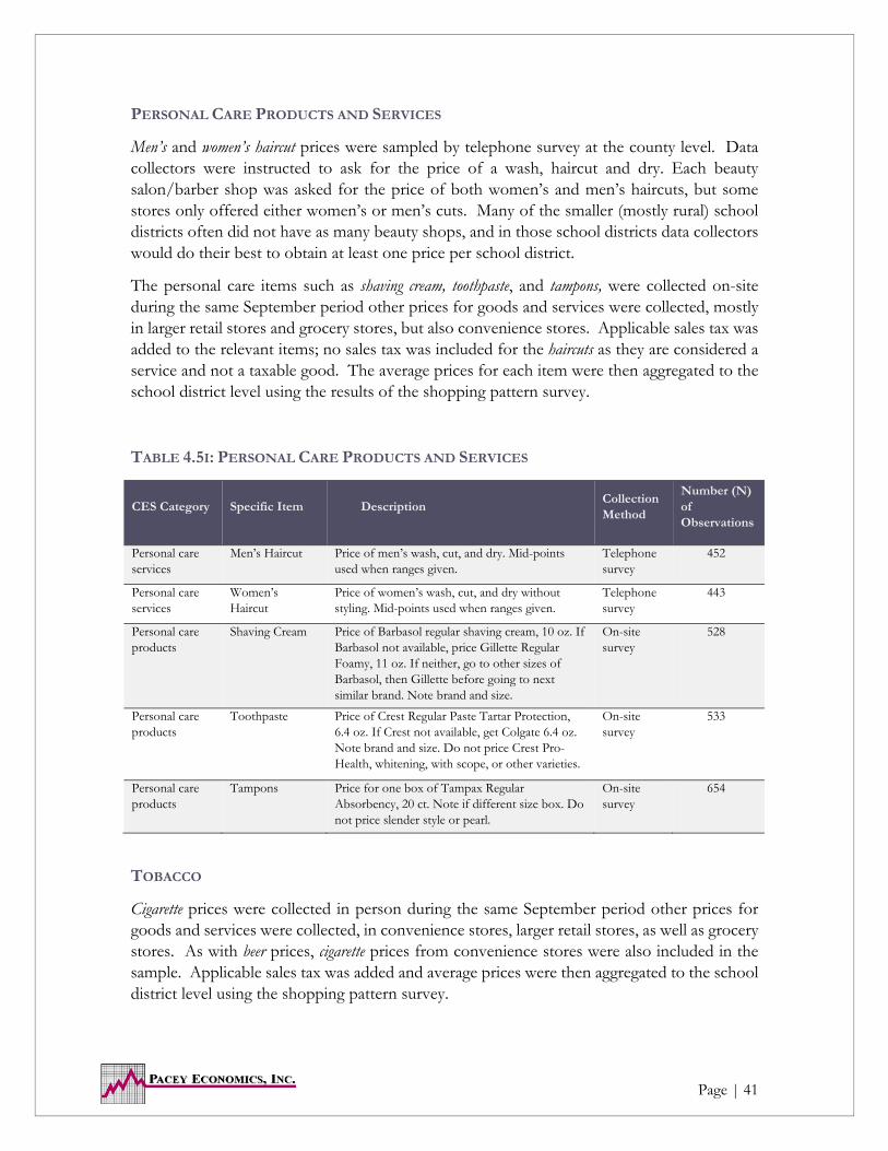
Page | 41 Page | 41

PERSONAL CARE PRODUCTS AND SERVICES

Men’s and women’s haircut prices were sampled by telephone survey at the county level. Data collectors were instructed to ask for the price of a wash, haircut and dry. Each beauty salon/barber shop was asked for the price of both women’s and men’s haircuts, but some stores only offered either women’s or men’s cuts. Many of the smaller (mostly rural) school districts often did not have as many beauty shops, and in those school districts data collectors would do their best to obtain at least one price per school district.

The personal care items such as shaving cream, toothpaste, and tampons, were collected on-site during the same September period other prices for goods and services were collected, mostly in larger retail stores and grocery stores, but also convenience stores. Applicable sales tax was added to the relevant items; no sales tax was included for the haircuts as they are considered a service and not a taxable good. The average prices for each item were then aggregated to the school district level using the results of the shopping pattern survey.

TABLE 4.5I: PERSONAL CARE PRODUCTS AND SERVICES

CES Category Specific Item Description Collection Method


Personal care services

Men’s Haircut Price of men’s wash, cut, and dry. Mid-points used when ranges given.

Telephone survey

452

Personal care services

Women’s Haircut

Price of women’s wash, cut, and dry without styling. Mid-points used when ranges given.

Telephone survey

443

Personal care products

Shaving Cream Price of Barbasol regular shaving cream, 10 oz. If Barbasol not available, price Gillette Regular Foamy, 11 oz. If neither, go to other sizes of Barbasol, then Gillette before going to next similar brand. Note brand and size.

On-site survey

528


Toothpaste Price of Crest Regular Paste Tartar Protection, 6.4 oz. If Crest not available, get Colgate 6.4 oz. Note brand and size. Do not price Crest Pro-Health, whitening, with scope, or other varieties.

On-site survey

533


Tampons Price for one box of Tampax Regular Absorbency, 20 ct. Note if different size box. Do not price slender style or pearl.

On-site survey

654

TOBACCO

Cigarette prices were collected in person during the same September period other prices for goods and services were collected, in convenience stores, larger retail stores, as well as grocery stores. As with beer prices, cigarette prices from convenience stores were also included in the sample. Applicable sales tax was added and average prices were then aggregated to the school district level using the shopping pattern survey.

Page | 42 Page | 42

TABLE 4.5J: TOBACCO

CES Category

Specific Item Description Collection Method


Tobacco

Cigarettes

Price for one carton (200 cigarettes) of Marlboro Filter, hard pack, flip-top cigarettes. If Marlboro is not available, price Camel cigarettes.

On-site survey

763

OTHER EXPENDITURE CATEGORIES

OTHER - PERSONAL INCOME TAXES

Personal income taxes were calculated for the “benchmark” family in each school district for federal and state income taxes and occupational/head taxes for relevant local jurisdictions. For federal income taxes, the standard deduction of $12,600 (for a married couple filing jointly) was compared to the itemized deduction calculated using mortgage interest and property taxes, as well as specific ownership taxes from vehicles, state income taxes, and cash contributions based on the CES, with the higher of the two deductions used for each school district. IRS Publication 936 was used to calculate the allowable limits on home mortgage interest deductions for high home value school districts (e.g., Aspen). Specific ownership taxes are calculated from the original Manufacturer’s Suggested Retail Price (MSRP) value for each vehicle, and the tax formula from the Colorado Motor Vehicle Law Resource Book. Colorado state income taxes are calculated from the formulas in publication, DR 1098 “Colorado Income Tax Withholding Tables for Employers”.

OTHER - READING, EDUCATION, CASH CONTRIBUTIONS, AND PERSONAL

INSURANCE AND PENSIONS

Mirroring previous cost of living studies, the major expenditure categories for Reading, Education, Miscellaneous Expenses, Cash Contributions, and Personal Insurance and Pensions were not sampled in this 2015 Cost of Living study. Similar to the previous studies, these expenditure categories were expected to be constant for the relevant “benchmark” family and were thus held constant for all school districts. No significant geographic variation or trends were expected to be seen for these goods, and the final costs allocated across the school districts came directly from the “benchmark” families spending level calculated for each category from the Consumer Expenditure Survey.

Page | 43 Page | 43

4.6 IDENTIFYING WHERE GOODS AND SERVICES ARE PURCHASED

As noted in Section 2, to measure the cost of living or a change in the cost of living for a school district it is also necessary to know where households purchase their goods and services. That is, if every resident in a school district made all of their purchases within a school district, calculating the cost of living in that school district would be relatively straightforward. However, this is not the case. Often residents leave their school district to make purchases, either because they can obtain a better price or better selection, another area is more convenient, or an item is simply not available in their school district. Because prices will vary across school district boundaries (sometimes materially), it was necessary to understand these geographic shopping patterns in order to develop the actual cost of living in each school district.

In the 2007, 2009, and 2011 studies a survey of residents was commissioned by the Colorado Legislative Council to gather input about the actual location of the purchases of goods and services. The data from these surveys, in conjunction with mathematical modeling methods, were used to construct a geographic shopping matrix describing where the residents of each school district typically purchase particular products (i.e., what percentage of purchases are made in the home school district, in each neighboring school district, online, etc.).

The 2013 study and this 2015 study continued to use this same shopping pattern survey for most goods and services. However, in addition to using the shopping pattern survey, the 2015 study also implemented an alternative, relatively sophisticated statistical procedure called Kriging, in which it is assumed that the probability of purchasing an item is inversely related to the distance from the school district to the store or, for purchases not available in the area, the likelihood the goods and services are purchased in the stores closest in proximity. That is, individuals may purchase items anywhere in the state, but are most likely to purchase from a store that is close by and/or in their school district, and are least likely to purchase from a store that is far away from their school district. As the price of certain services previously available which could then be tracked in the shopping pattern survey were no longer available, this alternative Kriging method was required to estimate average district prices. When comparing outcomes with the Kriging procedure to the 2013 data, we found the results to be similar, adding credibility to the shopping pattern survey as well as the potential opportunity for a more cost effective methodology for shopping purchase probabilities in future surveys. Appendix D further elaborates on the Kriging procedure.

ALLOCATING CITY/COUNTY DATA

Data collected with a specific address (e.g., field survey data, call data) can be linked directly to the school district in which it was gathered. However, other data was available only at the city level (e.g., city sales tax) or at the county level (e.g., county sales tax). As the shopping patterns survey links school district to school district, the city/county data must be mapped to school districts before the shopping patterns survey can be applied. City/county data were mapped to school districts on a pro rata

Page | 44 Page | 44

basis. For example, if 40% of goods and services purchased in a given school district was in County A, and 60% was in County B, then the school district county sales tax was computed as 40% of County A tax plus 60% of County B tax. In order to implement this methodology, it was necessary to determine what percent of each school district lies in each county. As population data were not available on a school district-by-county basis, Pacey Economics, Inc. determined a reasonable proxy was to use the number of businesses (available because the Hoover’s, Inc. business data had been mapped to both school district, city, and county) as the basis of proportionality, under the logic that business centers and population centers tend to be co-located.

Page | 45 Page | 45

4.7 DEVELOPING FINAL COST OF LIVING MEASURES

After the collection of all pricing data, two major steps were taken to develop the final cost of living measures. First, the price data for the “typical” market basket of goods and services was integrated with the shopping pattern survey (or Kriging method as discussed in the previous section) in order to develop prices for each school district that reflect where individual residents in the school district purchase their items. Second, annual expenditures were calculated by determining the ratio of the school district average price to the statewide average price for each good and then multiplying by the “typical” expenditure on that item according to the Consumer Expenditure Survey. This second step scales up costs so that the limited numbers of grocery items (for example) for which data were collected represent the full expenditures for food for the “benchmark” household. Each of these steps is described in further detail below.

INTEGRATING PRICE DATA WITH THE SHOPPING PATTERN SURVEY

While price data was primarily collected at the city or county level, school districts do not usually correlate to these geographic boundaries nor is the “benchmark” household likely to confine their buying habits to that of the school district in which they live. Consumers have a variety of purchasing options including:

purchasing costly items such as automobiles from a more populated geographic region;

purchasing items online;

consumers living in a school district near a metropolitan area may shop in their school district for some goods and services and in the metropolitan area for other goods and services; and

consumers residing in school districts in more rural areas with a substantial distance from a metropolitan area may still do a significant percentage of their buying in more urban areas.

Clearly, if households shop outside of the school district in which they live, the prices for these commodities need to be tracked to the location of the purchase in order to properly evaluate a cost of living measure for any given school district. To evaluate the shopping patterns of the “benchmark” household, surveys were conducted as part of the 2007, 2009, and 2011 cost of living studies. These surveys sought to determine the “benchmark” family’s spending within and/or outside of the school district in which they reside. These surveys, referred to as the shopping pattern surveys, were compiled by contacting households across the state and inquiring where households in each school district most recently purchased selected items from the major expenditure categories. Based upon the

Page | 46 Page | 46

household survey responses, the consultants for the past several cost of living studies developed matrices which apportion shopping activity by geographic locations for each school district. Based on the expectation of limited changes in the shopping patterns of the “benchmark” household over the past several years and the recommendation from the Colorado Legislative Council, the 2015 study continued to utilize these shopping pattern matrices. Importantly, as certain data sources were no longer available (e.g., homeowner’s and vehicle insurance), the shopping pattern survey provided a foundation to implement the Kriging method discussed earlier.

Integrating the results of the most recent shopping pattern surveys allowed for allocating costs for goods and services to the “benchmark” household in a particular school district in order to more accurately assess the overall annual expenditures for the “market basket”. For example, as noted in and consistent with earlier studies, 56 percent of the households residing in the Rangely school district indicated that they purchased groceries most of the time in Grand Junction while 44 percent of the respondents indicated they did most of their grocery shopping in Rangely. Thus, the school district average price for Food at Home required weighting the average price in Grand Junction by 56 percent and the average price in Rangely by 44 percent. The shopping pattern survey provided responses to questions regarding shopping habits for grocery items, household products, alcohol, clothing, gasoline, car maintenance and repairs, movie tickets, haircuts, dining out at restaurants, and shopping for larger products such as a furniture item, mattress, or appliance as well as televisions.

CALCULATING ANNUAL EXPENDITURES

To obtain the annual expenditure for a particular item in a given school district, it was necessary to find the average price for each school district, incorporating the appropriate city, county, and/or state tax rates. Prices only available at the city or county level were aggregated to the school district level. This procedure was repeated for each item and category for all 178 school districts. Mirroring the methodology used since the 2007 cost of living study, the majority of the market basket items were sampled by school district. This helped to ensure that all final cost of living data was specific to an exact school district. In a few cases, the data was only available at a county or region level, and needed to be aggregated to school districts based on location. Utilities prices, day care prices, and insurance prices are a few of the cases where data were available at the county or region level and were aggregated to school districts.

As population data are not available on a school district-by-county basis, Pacey Economics, Inc. determined a reasonable proxy was to use the number of businesses (available because the Hoover’s, Inc. business data had been mapped to both school district, city, and county) as the basis of proportionality, under the logic that business centers and population centers tend to be co-located.

Once a school district average price for a given item has been determined, a statewide average price by item can be calculated. The statewide average price was based on the

Page | 47 Page | 47

average price in each school district weighted by the teacher population for each school district.

The school district’s price for a particular item relative to the statewide average price for that item can then be determined by taking the ratio of the school district average price relative to the statewide average price. This ratio was then multiplied by the average annual expenditure for the item per information from the Consumer Expenditure Survey regarding the “typical” expenditures of the “benchmark” household.

This procedure, repeated for each item was then aggregated across the particular school district to obtain the school district’s total annual expenditures for a particular category. Total annual expenditures for each school district are the summation of annual totals for each major expenditure category.

CALCULATING CONFIDENCE INTERVALS

Confidence intervals were calculated for most expenditure categories using the same methodology as in past reports. The goal of the confidence intervals is to reflect the uncertainty arising from the fact that every store in the state is not visited, but that random sampling was used to collect data. For each item sampled and for each school district, the variance of the average price was computed. These variances were weighted by the shopping patterns and then aggregated over items in a category, and a confidence interval was calculated for the category as a whole. Details of the statistical methods involved are provided in Appendix C.

Essentially, large confidence intervals reflect a large variance of the mean, which means there is a large variability in the prices collected and/or relatively few prices were collected. In some cases, variability in the error may be reduced by additional sampling in those school districts; however, this is only likely to be true in large school districts where the universe of stores available to sample from is large. In general, the confidence intervals are relatively narrow, suggesting that additional sampling is not needed. It should be noted that factors other than the variability of the mean school district price (e.g., the shopping pattern survey) will affect uncertainty in the cost of living indices, but currently no additional factors are incorporated in the confidence interval estimates. Of note, incorporating these other factors will not impact the conclusions regarding the need for additional sampling.

See Appendix C for a more detailed discussion of statistical measures used in this study.

Page | 48

APPENDIX A: RESULTS BY RANK AND DETAILED MAPS

Appendix A includes Table A.1 which identifies the average annual expenditures for the “archetypical” household in order by rank, while Figures A.1 through A.6 present the visual results for the six largest expenditure categories: 1) Food, 2) Apparel, 3) Entertainment, 4) Transportation, 5) Housing, and 6) Healthcare.

As noted earlier in this report, the index value is the ratio of the cost of the specific expenditure category in each school district to the statewide average cost of the specific expenditure category market basket. An index value greater than 100 means that school district is more expensive than average while a value less than 100 reflects a less expensive than average school district. In these maps, Figures A.1 through A.6, shades of green (below 100) represent school districts that have annual expenditures below the statewide average while shades of blue (above 100) identify school districts with higher than the statewide average. Again, the lightest shades of green represent the lowest cost of the specific expenditure category and as the green darkens the expenditure for the specific category is moving toward the statewide average. The lighter shades of blue are at or near the statewide average and the darkest blue identifies the school districts with the highest expenditures for each specific category.

In addition, electronically available spreadsheets provide detail for the average annual expenditures for each of the underlying categories and/or subcategories for 2015 as well as the 2013 recalibrated expenditures.

Upon investigating the detailed data on expenditures, Pacey Economics, Inc. found the “benchmark” household spending less, on average, for Alcoholic beverages, Tobacco, and Transportation in 2015 than in 2013, although these reductions are fairly nominal. Fairly large expenditure increases for Healthcare and Personal taxes are noted between 2013 and 2015. As noted in Section 4.3, the increase in Personal taxes is due to changes in methodology implemented by the BLS for the 2014 CES, and as such, not likely due to any real change in Personal Taxes other than that associated with increases in household income. Healthcare costs in the rural areas increased substantially, likely due to the implementation of the Affordable Care Act (popularly referred to as ObamaCare), allowing for an increase in access participation with healthcare providers but at increased costs for these rural school districts.

Not surprisingly, Pacey Economics, Inc. saw the most price variation in the Apparel category, likely associated with a wider range of product quality (perceived or real) for (or access to) these items, e.g., women’s yoga pants, men’s dress shirt, etc.

In the Food category, Pacey Economics, Inc. found the combined expenditures of Food at Home and Food Away from Home rose, on average, similar to an inflationary increase with CES noting similar expenditure share between 2013 and 2015. However, Pacey Economics, Inc. did note some school districts, especially in the rural areas, had a greater increase in Food at Home vis-à-vis Food Away from Home.

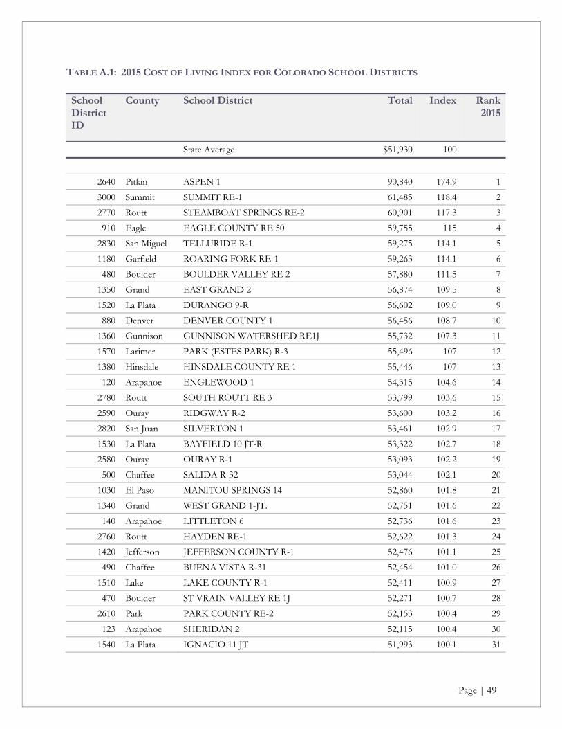
Page | 49

TABLE A.1: 2015 COST OF LIVING INDEX FOR COLORADO SCHOOL DISTRICTS School District ID

County School District Total Index Rank 2015


2640 Pitkin ASPEN 1 90,840 174.9 1

3000 Summit SUMMIT RE-1 61,485 118.4 2

2770 Routt STEAMBOAT SPRINGS RE-2 60,901 117.3 3

910 Eagle EAGLE COUNTY RE 50 59,755 115 4

2830 San Miguel TELLURIDE R-1 59,275 114.1 5

1180 Garfield ROARING FORK RE-1 59,263 114.1 6

480 Boulder BOULDER VALLEY RE 2 57,880 111.5 7

1350 Grand EAST GRAND 2 56,874 109.5 8

1520 La Plata DURANGO 9-R 56,602 109.0 9

880 Denver DENVER COUNTY 1 56,456 108.7 10

1360 Gunnison GUNNISON WATERSHED RE1J 55,732 107.3 11

1570 Larimer PARK (ESTES PARK) R-3 55,496 107 12

1380 Hinsdale HINSDALE COUNTY RE 1 55,446 107 13

120 Arapahoe ENGLEWOOD 1 54,315 104.6 14

2780 Routt SOUTH ROUTT RE 3 53,799 103.6 15

2590 Ouray RIDGWAY R-2 53,600 103.2 16

2820 San Juan SILVERTON 1 53,461 102.9 17

1530 La Plata BAYFIELD 10 JT-R 53,322 102.7 18

2580 Ouray OURAY R-1 53,093 102.2 19

500 Chaffee SALIDA R-32 53,044 102.1 20

1030 El Paso MANITOU SPRINGS 14 52,860 101.8 21

1340 Grand WEST GRAND 1-JT. 52,751 101.6 22

140 Arapahoe LITTLETON 6 52,736 101.6 23

2760 Routt HAYDEN RE-1 52,622 101.3 24

1420 Jefferson JEFFERSON COUNTY R-1 52,476 101.1 25

490 Chaffee BUENA VISTA R-31 52,454 101.0 26

1510 Lake LAKE COUNTY R-1 52,411 100.9 27

470 Boulder ST VRAIN VALLEY RE 1J 52,271 100.7 28

2610 Park PARK COUNTY RE-2 52,153 100.4 29

123 Arapahoe SHERIDAN 2 52,115 100.4 30

1540 La Plata IGNACIO 11 JT 51,993 100.1 31

Page | 50

TABLE A.1: 2015 COST OF LIVING INDEX FOR COLORADO SCHOOL DISTRICTS (CONT’D) School District ID



1550 Larimer POUDRE R-1 51,885 99.9 32

1195 Garfield GARFIELD RE-2 51,867 100 33

900 Douglas DOUGLAS COUNTY RE 1 51,773 99.7 34

920 Elbert ELIZABETH C-1 51,702 99.6 35

70 Adams WESTMINSTER 50 51,689 100 36

2020 Moffat MOFFAT COUNTY RE:NO 1 51,630 99.4 37

60 Adams STRASBURG 31J 51,563 99.3 38

3100 Weld WINDSOR RE-4 51,507 99.2 39

2600 Park PLATTE CANYON 1 51,491 99.2 40

130 Arapahoe CHERRY CREEK 5 51,342 98.9 41

540 Clear Creek CLEAR CREEK RE-1 51,333 98.9 42

2010 Mineral CREEDE CONSOLIDATED 1 50,852 97.9 43

180 Arapahoe ADAMS-ARAPAHOE 28J 50,834 97.9 44

220 Archuleta ARCHULETA COUNTY 50 JT 50,802 97.8 45

1080 El Paso LEWIS-PALMER 38 50,649 97.5 46

1020 El Paso CHEYENNE MOUNTAIN 12 50,594 97.4 47

1160 Fremont COTOPAXI RE-3 50,473 97.2 48

3020 Teller WOODLAND PARK RE-2 50,434 97.1 49

50 Adams BENNETT 29J 50,405 97.1 50

3110 Weld JOHNSTOWN-MILLIKEN RE-5J 50,312 96.9 51

1560 Larimer THOMPSON R-2J 50,282 96.8 52

3085 Weld EATON RE-2 50,252 97 53

860 Custer CUSTER COUNTY SCHOOL DISTRICT C-1 50,216 96.7 54

2700 Pueblo PUEBLO COUNTY 70 50,172 96.6 55

20 Adams ADAMS 12 FIVE STAR SCHOOLS 50,059 96 56

1400 Huerfano LA VETA RE-2 49,973 96.2 57

870 Delta DELTA COUNTY 50(J) 49,949 96.2 58

1140 Fremont CANON CITY RE-1 49,940 96.2 59

2180 Montrose MONTROSE COUNTY RE-1J 49,870 96.0 60

3140 Weld WELD COUNTY S/D RE-8 49,846 96 61

2070 Montezuma MANCOS RE-6 49,841 96.0 62

Page | 51




1330 Gilpin GILPIN COUNTY RE-1 49,806 95.9 63

2000 Mesa MESA COUNTY VALLEY 51 49,794 95.9 64

1040 El Paso ACADEMY 20 49,765 95.8 65

1220 Garfield GARFIELD 16 49,697 95.7 66

1060 El Paso PEYTON 23 JT 49,632 95.6 67

950 Elbert ELBERT 200 49,584 95.5 68

2800 Saguache MOFFAT 2 49,449 95.2 69

930 Elbert KIOWA C-2 49,418 95.2 70

2840 San Miguel NORWOOD R-2J 49,415 95.2 71

1990 Mesa PLATEAU VALLEY 50 49,310 95.0 72

2515 Morgan WIGGINS RE-50(J) 49,287 94.9 73

40 Adams BRIGHTON 27J 49,271 94.9 74

10 Adams MAPLETON 1 49,261 94.9 75

1150 Fremont FREMONT RE-21 49,238 94.8 76

1828 Logan VALLEY RE-1 49,237 94.8 77

3080 Weld WELD COUNTY RE-1 49,206 94.8 78

1010 El Paso COLORADO SPRINGS 11 49,186 94.7 79

1600 Las Animas HOEHNE REORGANIZED 3 49,183 94.7 80

1410 Jackson NORTH PARK R-1 49,128 94.6 81

2055 Montezuma DOLORES RE-4A 49,124 94.6 82

3090 Weld KEENESBURG RE-3(J) 49,116 94.6 83

2720 Rio Blanco RANGELY RE-4 49,065 94.5 84

3120 Weld GREELEY 6 49,059 94.5 85

2710 Rio Blanco MEEKER RE1 49,019 94.4 86

3010 Teller CRIPPLE CREEK-VICTOR RE-1 48,981 94.3 87

30 Adams ADAMS COUNTY 14 48,972 94.3 88

190 Arapahoe BYERS 32J 48,931 94.2 89

2395 Morgan BRUSH RE-2(J) 48,866 94.1 90

110 Alamosa SANGRE DE CRISTO RE-22J 48,807 94.0 91

2730 Rio Grande DEL NORTE C-7 48,646 93.7 921Fremont RE-2 was previously identified as Florence RE-2 in the 2013 study.

Page | 52




990 El Paso WIDEFIELD 3 48,611 93.6 93

2190 Montrose WEST END RE-2 48,592 94 94

1110 El Paso FALCON 49 48,479 93.4 95

2690 Pueblo PUEBLO CITY 60 48,479 93.4 96

2405 Morgan FORT MORGAN RE-3 48,440 93 97

1000 El Paso FOUNTAIN 8 48,415 93.2 98

2035 Montezuma MONTEZUMA-CORTEZ RE-1 48,384 93.2 99

1580 Las Animas TRINIDAD 1 48,335 93.1 100

1590 Las Animas PRIMERO REORGANIZED 2 48,309 93.0 101

3130 Weld PLATTE VALLEY RE-7 48,178 92.8 102

1500 Kit Carson BURLINGTON RE-6J 48,111 92.6 103

980 El Paso HARRISON 2 48,087 92.6 104

2505 Morgan WELDON VALLEY RE-20(J) 48,069 92.6 105

3145 Weld AULT-HIGHLAND RE-9 48,026 92 106

3200 Yuma YUMA 1 48,012 92.5 107

1860 Logan BUFFALO RE-4 47,956 92.3 108

3210 Yuma WRAY RD-2 47,924 92.3 109

1050 El Paso ELLICOTT 22 47,909 92.3 110

1850 Logan FRENCHMAN RE-3 47,902 92.2 111

890 Dolores DOLORES COUNTY RE NO.2 47,885 92.2 112

2790 Saguache MOUNTAIN VALLEY RE 1 47,761 92.0 113

170 Arapahoe DEER TRAIL 26J 47,687 91.8 114

1490 Kit Carson BETHUNE R-5 47,653 91.8 115

1980 Mesa DE BEQUE 49JT 47,615 91.7 116

970 El Paso CALHAN RJ-1 47,606 91.7 117

1450 Kit Carson ARRIBA-FLAGLER C-20 47,447 91.4 118

1870 Logan PLATEAU RE-5 47,377 91.2 119

2740 Rio Grande MONTE VISTA C-8 47,329 91.1 120

100 Alamosa ALAMOSA RE-11J 47,326 91.1 121

2630 Phillips HAXTUN RE-2J 47,290 91.1 122

1120 El Paso EDISON 54 JT 47,282 91.0 123

Page | 53




2570 Otero SWINK 33 47,262 91.0 124

740 Costilla SIERRA GRANDE R-30 47,258 91.0 125

1480 Kit Carson STRATTON R-4 47,180 90.9 126

1620 Las Animas AGUILAR REORGANIZED 6 47,108 90.7 127

3050 Washington OTIS R-3 47,021 91 128

3030 Washington AKRON R-1 47,016 90.5 129

2660 Prowers LAMAR RE-2 46,979 90.5 130

1130 El Paso MIAMI/YODER 60 JT 46,866 90.2 131

960 Elbert AGATE 300 46,829 90.2 132

3060 Washington LONE STAR 101 46,824 90.2 133

3040 Washington ARICKAREE R-2 46,714 90.0 134

1390 Huerfano HUERFANO RE-1 46,694 89.9 135

1460 Kit Carson HI-PLAINS R-23 46,659 89.8 136

2750 Rio Grande SARGENT RE-33J 46,611 89.8 137

2620 Phillips HOLYOKE RE-1J 46,605 89.7 138

3220 Yuma IDALIA RJ-3 46,599 89.7 139

2670 Prowers HOLLY RE-3 46,597 89.7 140

520 Cheyenne CHEYENNE COUNTY RE-5 46,572 89.7 141

2530 Otero ROCKY FORD R-2 46,562 89.7 142

2862 Sedgwick JULESBURG RE-1 46,505 90 143

2680 Prowers WILEY RE-13 JT 46,480 90 144

3146 Weld BRIGGSDALE RE-10 46,431 89.4 145

290 Bent LAS ANIMAS RE-1 46,420 89.4 146

770 Crowley CROWLEY COUNTY RE-1-J 46,365 89.3 147

2540 Otero FOWLER R-4J 46,355 89.3 148

3070 Washington WOODLIN R-104 46,321 89.2 149

3230 Yuma LIBERTY J-4 46,295 89.1 150

1440 Kiowa PLAINVIEW RE-2 46,281 89.1 151

2560 Otero CHERAW 31 46,198 89.0 152

230 Baca WALSH RE-1 46,134 88.8 153

580 Conejos SOUTH CONEJOS RE-10 46,048 88.7 154

Page | 54




270 Baca CAMPO RE-6 46,023 88.6 155

310 Bent MC CLAVE RE-2 46,002 89 156

640 Costilla CENTENNIAL R-1 45,993 89 157

2520 Otero EAST OTERO R-1 45,968 89 158

2650 Prowers GRANADA RE-1 45,947 88.5 159

1070 El Paso HANOVER 28 45,916 88.4 160

510 Cheyenne KIT CARSON R-1 45,863 88.3 161

1430 Kiowa EADS RE-1 45,687 88.0 162

250 Baca SPRINGFIELD RE-4 45,663 87.9 163

940 Elbert BIG SANDY 100J 45,647 87.9 164

2535 Otero MANZANOLA 3J 45,581 87.8 165

560 Conejos SANFORD 6J 45,570 87.8 166

260 Baca VILAS RE-5 45,535 87.7 167

1750 Las Animas BRANSON REORGANIZED 82 45,507 87.6 168

2865 Sedgwick REVERE SCHOOL DISTRICT1 45,502 87.6 169

1790 Lincoln LIMON RE-4J 45,498 87.6 170

1780 Lincoln GENOA-HUGO C113 45,295 87.2 171

2810 Saguache CENTER 26 JT 45,244 87.1 172

550 Conejos NORTH CONEJOS RE-1J 45,039 86.7 173

1760 Las Animas KIM REORGANIZED 88 45,020 86.7 174

240 Baca PRITCHETT RE-3 44,962 87 175

3147 Weld PRAIRIE RE-11 44,880 86.4 176

1810 Lincoln KARVAL RE-23 44,858 86.4 177

3148 Weld PAWNEE RE-12 44,350 85.4 1781Revere School District was previously identified as Platte Valley Re-3 in the 2013 study.

Page | 55

FIGURE A.1: MAP OF FOOD INDEX FOR COLORADO SCHOOL DISTRICTS, 2015

Page | 56

FIGURE A.2: MAP OF APPAREL INDEX FOR COLORADO SCHOOL DISTRICTS, 2015

Page | 57

FIGURE A.3: MAP OF ENTERTAINMENT INDEX FOR COLORADO SCHOOL DISTRICTS, 2015

Page | 58

FIGURE A.4: MAP OF TRANSPORTATION INDEX FOR COLORADO SCHOOL DISTRICTS, 2015

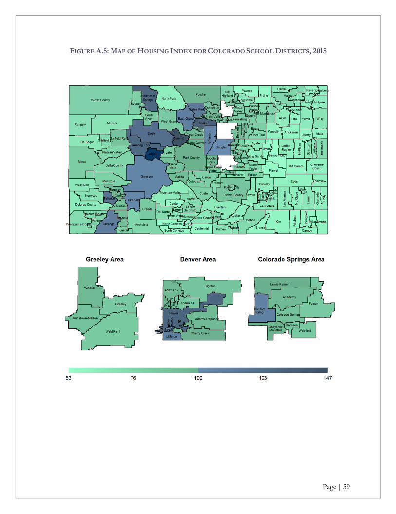
Page | 59

FIGURE A.5: MAP OF HOUSING INDEX FOR COLORADO SCHOOL DISTRICTS, 2015

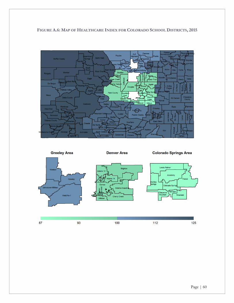
Page | 60

FIGURE A.6: MAP OF HEALTHCARE INDEX FOR COLORADO SCHOOL DISTRICTS, 2015

Page | 61

APPENDIX B: DETAILED METHODOLOGICAL DISCUSSION – DATA

COLLECTION

In Section 4 of the report, a methodological overview is provided regarding the data collection methods for each major expenditure category. Appendix B provides additional detail on those topics for the interested reader, specifically the change in sampling methodology from the previous study.

SAMPLING METHODOLOGY

The ultimate goal of the study is to construct cost-of-living measures for each of Colorado’s 178 school districts. These cost-of-living measures are based on the average price of specific goods and services (e.g., bananas, bread, pizza, shoes, women’s haircuts, etc.) in each school district. One strategy for determining the average prices would be to take a census; that is, to visit every business that sells the good, for example, milk. While highly accurate, taking a census is also prohibitively expensive and time-consuming. The alternative to a census is to take a sample, in which a subset of businesses are visited, and the price of milk in the businesses sampled is used to estimate the price of milk across the entire school district.

The first step in drawing a sample is to determine the sample size, i.e., how many businesses in each school district to visit. There are trade-offs in determining sample size: as the sample size increases (more businesses are visited), the accuracy of the final estimate increases but so does the cost and time required to take the sample. The relationship between accuracy and sample size is driven by the underlying variability in prices within school districts. For example, there is more variability in the price of women’s haircuts than in the price of milk. In the 2013 study, the price of milk ranged from $1.99 to $5.49 (a range of $3.50) while the price of a women’s haircut ranged from $10.00 to $75.00 (a range of $65.00). Because of greater price variability, the accuracy of women’s haircut price estimates will be less than that of milk, given equal sample sizes.

One of the great advantages of the repetitive nature of the cost of living study is that the data from the 2013 study can be analyzed to determine price variability, and hence, the relationship between sample size and accuracy. The results of this analysis are presented in Table B.1 below. The first column gives items ordered by relative variability, the second column (labeled “Average Price”) provides the average price of each item across all school districts, while the third column (labeled “Price Standard Deviation”) notes the standard deviation of price (a statistical measure of variability) within the school districts. The last five columns gives the maximum percent error in the estimated average price for various sample sizes. For example, given the previous years if just one business in each school district is visited, and using the estimated standard deviations from the 2013 study, the maximum percent error in the milk price estimate is 26%, while if 10 businesses are visited, the maximum percent error falls to 8%.

An important sampling property illustrated in Table B.1 is that the value of adding more visits to the sample (value in terms of accuracy) continually falls. For milk, increasing the sample size from 1

Page | 62

business to 10 businesses increases accuracy by 8%, but adding another 10 businesses (for a total sample size of 20) increases accuracy by only another 1%.

After studying Table B.1, Pacey Economics, Inc. concluded that a sample of 10 businesses per item per school district was an appropriate target, with larger samples providing limited gains in accuracy.

TABLE B.1: PRICE VARIABILITY AND SAMPLE ACCURACY

Maximum Percent Error Sample Size

Item Average Price Price Standard

Deviation 1 5 10 15 20 gasoline $3.42 $0.11 7% 3% 2% 2% 1% beer $8.26 $0.50 12% 5% 4% 3% 3% beef $3.73 $0.32 17% 8% 5% 4% 4% television $300.90 $26.08 17% 8% 5% 4% 4% cigarettes $56.04 $5.92 21% 9% 7% 5% 5% refrigerator $1,409.31 $161.26 23% 10% 7% 6% 5% milk $3.47 $0.45 26% 12% 8% 7% 6% laundry soap $8.55 $1.11 26% 12% 8% 7% 6% bananas $0.61 $0.08 27% 12% 8% 7% 6% waffles $2.30 $0.34 30% 13% 9% 8% 7% shaving cream $1.60 $0.27 34% 15% 11% 9% 8% coffee $5.24 $0.91 35% 15% 11% 9% 8% batteries $4.73 $0.83 35% 16% 11% 9% 8% front end alignment $74.43 $13.40 36% 16% 11% 9% 8% peaches $1.29 $0.23 36% 16% 11% 9% 8% toothpaste $2.54 $0.46 36% 16% 11% 9% 8% movie tickets $9.18 $1.83 40% 18% 13% 10% 9% oil change $44.74 $9.64 43% 19% 14% 11% 10% pizza $11.14 $2.41 43% 19% 14% 11% 10% tampons $4.26 $1.01 47% 21% 15% 12% 11% pantyhose $4.63 $1.11 48% 21% 15% 12% 11% green beans $0.86 $0.21 48% 22% 15% 12% 11% potatoes $5.13 $1.24 48% 22% 15% 12% 11% cheeseburger $8.14 $2.01 49% 22% 16% 13% 11% men's haircut $19.63 $5.06 52% 23% 16% 13% 12% steak $20.37 $5.45 53% 24% 17% 14% 12% bread $1.83 $0.49 54% 24% 17% 14% 12% spaghetti $1.39 $0.38 54% 24% 17% 14% 12% chicken $1.36 $0.37 55% 25% 17% 14% 12% pet food $0.70 $0.21 60% 27% 19% 15% 13% women's haircut $27.38 $8.84 65% 29% 20% 17% 14% soup $1.21 $0.41 68% 31% 22% 18% 15% men's t-shirt $13.19 $5.62 85% 38% 27% 22% 19% shoes $30.47 $15.18 100% 45% 32% 26% 22% men's dress shirt $26.07 $13.06 100% 45% 32% 26% 22% women's cardigan $26.66 $14.03 105% 47% 33% 27% 24%

Page | 63

The second key step in drawing a sample is to determine the sampling frame, i.e., the list of businesses from which the sample for a particular item is drawn. Our core source of business information is Hoover’s Inc., a subsidiary of The Dun & Bradstreet Corporation. Hoover’s, Inc. provides information on businesses including name, address, phone number, number of employees, and NAICS classification (North American Industrial Classification System, the standard used by Federal statistical agencies in classifying business establishments by industry; for example the code “445120” identifies a business as being a convenience business).

Hoovers, Inc. identifies over 400,000 businesses in the state of Colorado. For each item, a subset of those businesses that are likely to carry that item was identified and used as the sampling frame. For example, the sampling frame for milk (one of the most widely available items) included grocery stores (e.g., King Soopers), supercenters (e.g., Walmart), and convenience stores. At the other extreme, the sampling frame for front end alignments consisted solely of auto repair shops.

It is helpful to compare the Pacey Economics, Inc. target sample size of 10 with the sample sizes used in previous studies. The 2013 study uses a target of the larger of five businesses or five percent of the sampling frame. So, the Pacey Economics, Inc. sample size is larger if there are fewer than 200 businesses selling a particular item in a particular school district and is smaller if there are more than 200 businesses. We would remark that the 2013 study used a rather unusual statistical sampling methodology, in which the sample size increases with the sampling frame. The reason this methodology is uncommon is that as the size of the sampling frame grows, it is not necessary to increase the size of the sample to maintain a given level of accuracy. That is, a sample size of 10 gives virtually the same accuracy if there are one hundred, one thousand, or one million businesses in the sampling frame.

Further, not only is it not necessary to increase the sample size as the sampling frame grows, but it is possible to reduce the sample size if the sampling frame is quite small. For example, if there are only 20 businesses in the sampling frame, a sample size of 7 provides the same accuracy as a sample of 10 from a large sampling frame, and this is the specific methodology used by Pacey Economics, Inc.: for a given sampling frame, the sample size is the value that gives the same accuracy as a sample of 10 observations from a very large frame. We did make two modifications to this methodology to maintain consistency with previous studies: 1) if there were five or fewer businesses in the sampling frame, we included them all in the sample (as did the 2013 study), and 2) if our sample size was smaller than the number of observations in the 2013 study, we increased our sample size to that value. This methodology ensured that we target at least as much data as in the 2013 study, and that we make the most efficient use of the data in terms of the accuracy of the cost of living measure for each school district.

Given the sample size and the sampling frame, the final step is to draw a random sample. In a simple random sample, each business in the sampling frame has an equally likely chance of being selected. Randomness is important so that the sample properly reflects the underlying population, and so that statistical methods can be used to assess the accuracy of the price estimates and of the final cost of living measures. A slightly more complex sampling method is used in this study to recognize that shoppers are more likely to purchase items from large stores than from small stores. In particular, the probability of a business being selected in a sample is proportional to the number of business employees, a proxy for business size.

Page | 64

As previously noted, about one-quarter of the school districts have no grocery stores, and another quarter only have one. Again, it is not surprising the school districts with limited shopping opportunities are in rural locations. It has also been our experience that businesses in the rural locations tend to be more fluid, with rural areas having a greater mismatch between the businesses actually operating as identified by our data collection team and those identified in in the Hoover’s, Inc. database.

Page | 65

APPENDIX C: STATISTICAL MEASURES USED IN THIS REPORT

Confidence intervals are calculated for most expenditure categories using the same methodology utilized in past reports. Confidence intervals reflect the uncertainty arising from the fact that every store in the state is not visited, but that random sampling is used to collect data.

To illustrate a confidence interval, consider a district that has 30 grocery stores and suppose that the average price of a loaf of bread in these 30 stores is actually $1.75. The only way to learn that the average price is $1.75 would be to visit every store, but this is an extremely wasteful use of time and resources. To learn about the price of bread in the district, it is much more cost-efficient to visit a random sample of the stores. Now, suppose that, based on the sampling methodology, 10 of the 30 stores were randomly selected and the price of a loaf of bread in those 10 stores was recorded. It is not expected that the average price of the bread in those 10 stores will be exactly $1.75 (the average in all 30 stores in the district), but it is expected that the average price in the random sample will be close to $1.75. The critical question is how close do we expect the average in the random sample of 10 stores to be to the average over all 30 stores. The answer is given by a confidence interval. The confidence interval is a range of values computed from the sample that we are quite sure contains the actual average price in all the stores. For example, the confidence interval might be $1.72 to $1.79; this is a fairly narrow range, and indicates that the sample mean price is likely quite close to the actual mean (average) price. A wider confidence interval might be $1.35 to $2.12; this wide range indicates that we are uncertain if the sample mean price is close or far from the actual mean (average) price.

The width of the confidence interval is dependent on two basic factors. The first is the underlying variability in the price of the item being measured. For example, bread is a fairly standard commodity readily available in grocery stores throughout the state, and its price variability is relatively small. On the other hand, men’s t-shirts are available in both discount stores as well as fashion stores, with a relatively large price variability. Other things held fixed, the confidence interval for bread will be relatively narrower than the confidence interval for men’s t-shirts. Price variability depends on the specific characteristics of the item, and cannot be controlled.

The second factor determining the width of the confidence interval is the size of the sample, with smaller samples resulting in wider confidence intervals (but costing less), and larger samples providing more narrow confidence intervals (but costing more). (Of course, if the number of sample points increases to the total number of stores in the district, the sample mean will be the actual mean, and the confidence interval has a zero width.) The dependence of the confidence interval on sample size is important because sample size, unlike price variability, is a factor that can be controlled. However, there is the dilemma of surveying: as the sample size increases so does accuracy, but the cost of conducting the survey also increases. As is emphasized in the statistical discussion of previous studies, the primary motivation of constructing confidence intervals in this study is to determine if additional sampling, with additional cost, is needed.

As sample size increases the degree of confidence in the estimated average also increases (reflected in a narrower confidence interval). However, increasing the sample gives less-than-proportionate increases in confidence. For example, doubling the sample size only reduces the width of the confidence interval

Page | 66

by 39%; quadrupling the sample size reduces the width of the confidence interval by 50%; and increasing the sample size eight times only reduces the width of the confidence interval by 65%. However, it is expected that the cost of drawing the sample will likely be proportional to sample size; doubling the sample will likely cost twice as much and quadrupling the sample will likely cost four times as much.

The expenditures in this study are the result of fairly complex calculations that depend on numerous factors including item average prices, shopping patterns survey data, expenditure share data, etc. While all these factors will contribute to variation in the final expenditure values, it is only sample size that can be controlled. Just as in previous studies, and because the issue being addressed is whether additional sampling is needed, the computed confidence intervals only reflect the variation in average prices (which depend on sample size). It should be emphasized that, as in previous studies, the reported confidence intervals do not reflect all sources of variation. Indeed, given the complexity of the calculations, and the lack of information on other sources of variation, etc., determining confidence intervals that include all sources of variability would be difficult to compute.

The specific methodology for computing the confidence intervals follows. Of note, this is the same logic used in the previous studies, but the following derivations are somewhat more straightforward.

Let be the mean price in the i’th district (i = 1,…,178).

Let be the mean prices weighted by the shopping patterns matrix:

where is the shares of purchases by teachers in the i’th district that are made in district j.

Let P be the state weighted-average price:

where is the share of teacher FTE’s (full-time equivalent) in the i’th district.

Finally, let be the total expenditures in the i’th district:

∗ 51,930 ∗

where c is the expenditure share of the item. Note that the expenditure has the properties that 1) it is proportional to the mean price in the i’th district (weighted by the shopping patterns survey) and 2) the average across districts (weighted by district FTE’s) is precisely the state average salary ($51,930) times the item expenditure share.

Let the mean of be and let the mean of P be and recall that , , and c (the shopping patterns matrix, the teacher FTE shares, and the expenditure shares) are taken as fixed. Using well-known approximations for the variance of a ratio, the variance of is:

Page | 67

1

21

, 51,930 ∗

(Of note, the 2013 study does not compute the first-order Taylor’s series expansion quite properly, with the 2013 expression for excluding the term involving the covariance between and P.)

The variance of is:

11

where is the population variance of the price of the item, is the total number of stores selling the item, and is the number of stores sampled. Then, given the assumed independence between and , the terms , , ,and are easily expressed given the summation

definitions. The estimated variance of is then computed using sample values for . , and , and the 95% confidence interval for is:

1.96 ∗

Of note, following previous studies, the term

1.96 ∗

is reported in Appendix A.

Examining the results in Appendix A, it appears that the confidence intervals are relatively narrow, with the implication that additional sampling is not likely to be an efficient use of state resources.

Page | 68

APPENDIX D: KRIGING

While some items (e.g., televisions) are not sold in every district, application of the shopping patterns survey generates a district price for those items. However, for other items (e.g., homeowner’s insurance, vehicle insurance), prices were not available in every district (as discussed in the body of the report), and using the shopping patterns survey is not appropriate when prices are based on geographic residence. For these prices, it was necessary to use spatial interpolation to obtain prices in each district.

Spatial interpolation uses data that is collected at certain geographic locations to predict values at other geographic locations. The most widely used method of spatial interpolation is known as Kriging (one more application of generalized least squares). Kriging is used in applications arising in many disciplines, ranging from predicting incomes to predicting disease to predicting mineral deposits. Kriging predications are based on weighted averages of the observed data, as is common in statistics. The weights are based on two fundamental factors. The first is the geographic distance between points, with observations closer to the prediction point getting a higher weight than observations far from the prediction point. The second weighting factor is related to the “smoothness” of the topography surrounding the prediction point. For example, the Aspen school district has some prices substantially greater than those in surrounding districts. In Kriging, those Aspen prices will be given a somewhat lower weight because they are unusually large (or, outliers). The specific methodology used to spatially interpolate the homeowner’s insurance and vehicle insurance values is simple Kriging using the krige function in the gstat package of the R statistical language.

As noted above, the shopping pattern survey is used to estimate district prices for many items. However, the shopping pattern survey has some limitations. One limitation is that the underlying samples are four years old, or older. Another limitation is that the data are likely to have substantial sampling error. This is simply a reflection of the magnitude of the problem: for each of the 178 school districts, how often purchases are made in each of the 178 school districts must be estimated, which translates into 31,684 estimates. However, it is not surprising that the shopping pattern data reveal that most purchases are made within the district of residence. This suggests simply using the price of the item in stores in the district as the district price. However, this creates the problem of what to use for items not sold in a district (e.g., televisions). Kriging provides a solution to this problem. Hence, an alternative to using the shopping patterns survey is to use district store prices when available, and to use Kriging to estimate prices when district store prices are not available. Figure F.1 plots the 2015 results computed using the shopping patterns survey (i.e., those reported in the body of this report) versus the 2015 results computed using the alternative (i.e., district store prices with missing data filled using Kriging). The plot shows a very strong correlation between the results, suggesting the alternative is a viable option. Of note, the alternative could be improved (i.e., a better match to the shopping pattern survey could be obtained) by analyzing the existing shopping patterns data to identify regional shopping centers (i.e., Grand Junction in the west, Denver in the east) and to incorporate this information into a Kriging methodology for all school districts.

Page | 69

Page | 70

APPENDIX E: RAW PRICING DATA FOR SELECTED PURCHASE

CATEGORIES

This appendix provides the raw pricing data that underpins the analysis. Readers receiving this report electronically will need to review an accompanying spreadsheet file, due to the volume of data.

.

Page | 71

APPENDIX F: SHOPPING PATTERNS SURVEY

This appendix provides the geographic shopping patterns matrix used in this analysis. In 2007, 2009, and 2011, the previous contractor conducted a survey of residents of each district to gather input about where they most recently purchased a series of goods. The data from these surveys, in conjunction with mathematical modeling methods, were used to construct a geographic shopping matrix describing where the residents of each school district typically purchase particular products (i.e., what proportion of purchases are made in the home district, in each neighboring district, online, etc.). The geographic shopping patterns matrix was not updated in 2013. Readers receiving this report will need to review an accompanying spreadsheet file due to the volume of data.

Page | 72

APPENDIX G: CONSUMER EXPENDITURE SURVEY

TABLE G.1: CONSUMER EXPENDITURE SURVEY

Table 3433. Consumer units of three people by income before taxes: Average annual expenditures and characteristics, Consumer Expenditure Survey, 2013-2014

Item $20,000

to $29,999

$30,000 to

$39,999

$40,000 to

$49,999

$50,000 to

$69,999

$70,000 and

more

Number of consumer units (in thousands) 1,710 1,837 1,739 3,100 8,320

Consumer unit characteristics:

Income before taxes $24,780 $34,988 $44,790 $59,455 $131,677

Income after taxes 27,846 35,858 43,295 55,694 110,482

Age of reference person 43.7 45.9 45.3 46.4 47.2

Average number in consumer unit:

People 3.0 3.0 3.0 3.0 3.0

Children under 18 .9 .7 .6 .6 .6

Adults 65 and older .3 .3 .3 .3 .2

Earners 1.3 1.4 1.7 1.7 2.1

Vehicles 1.4 1.7 2.0 2.3 2.8

Percent distribution:

Reference person: Men 40 40 40 48 54

Women 60 60 60 52 46

Housing tenure:

Homeowner 36 52 61 68 85

With mortgage 18 31 38 45 69

Without mortgage 19 21 23 23 16

Renter 64 48 39 32 15

Race of reference person:

Black or African-American 23 18 18 13 9

White, Asian, and all other races 77 82 82 87 91

Hispanic or Latino origin of reference person:

Hispanic or Latino 24 24 17 15 9

Not Hispanic or Latino 76 76 83 85 91

Education of reference person:

Page | 73

TABLE G.1: CONSUMER EXPENDITURE SURVEY (CONT’D)

Item $20,000

to $29,999

$30,000 to

$39,999

$40,000 to

$49,999

$50,000 to

$69,999

$70,000 and

more

Elementary (1-8) 7 6 6 4 1

High school (9-12) 49 46 42 33 21

College 43 47 52 63 78

Never attended and other b/ b/ c/ b/ b/

At least one vehicle owned or leased 85 89 92 97 98

Average annual expenditures $32,433 $37,507 $44,081 $52,210 $86,764

Food 5,116 5,730 6,872 6,970 10,094

Food at home 3,602 3,806 4,456 4,251 5,722

Cereals and bakery products 454 536 577 620 720

Cereals and cereal products 181 171 203 211 242

Bakery products 273 365 374 409 478

Meats, poultry, fish, and eggs 916 862 932 953 1,255

Beef 232 235 267 272 325

Pork 170 173 176 186 247

Other meats 110 129 118 131 172

Poultry 217 162 173 190 237

Fish and seafood 122 104 134 115 198

Eggs 65 60 65 59 76

Dairy products 393 339 455 458 586

Fresh milk and cream 178 140 164 176 202

Other dairy products 215 199 291 282 384

Fruits and vegetables 661 722 792 745 1,104

Fresh fruits 229 232 267 258 406

Fresh vegetables 194 220 255 221 367

Processed fruits 116 108 125 113 157

Processed vegetables 122 162 145 153 174

Other food at home 1,178 1,346 1,700 1,475 2,057

Sugar and other sweets 108 125 136 152 205

Fats and oils 88 116 144 126 161

Miscellaneous foods 580 703 919 736 1,076

Nonalcoholic beverages 391 386 460 444 541

Food prepared by consumer unit on out-of- town trips

a/ 12 a/ 16 40 17 75

Food away from home 1,514 1,924 2,416 2,719 4,372

Alcoholic beverages 253 204 302 302 691

Housing 11,933 14,124 15,279 16,705 26,579

Shelter 6,769 7,982 8,358 9,199 15,375

Owned dwellings 1,941 3,428 4,019 5,332 11,601

Mortgage interest and charges 944 1,906 2,154 2,783 6,521

Page | 74


Item $20,000

to $29,999

$30,000 to

$39,999

$40,000 to

$49,999

$50,000 to

$69,999

$70,000 and

more

Property taxes 573 982 1,198 1,563 3,248 Maintenance, repairs, insurance, other expenses

425 541 667 987 1,832

Rented dwellings 4,651 4,375 4,073 3,556 2,502

Other lodging 177 178 266 311 1,273

Utilities, fuels, and public services 3,255 3,788 4,148 4,424 5,410

Natural gas 298 367 417 415 598

Electricity 1,388 1,587 1,651 1,646 1,841

Fuel oil and other fuels a/ 57 84 136 154 244

Telephone services 1,075 1,274 1,480 1,658 1,981

Residential phone service, VOIP, and phone cards

265 300 376 393 453

Cellular phone service 810 974 1,104 1,265 1,528

Water and other public services 437 476 464 552 746

Household operations 604 725 901 1,182 2,315

Personal services 168 301 347 501 1,104

Other household expenses 436 425 554 681 1,212

Housekeeping supplies 490 522 547 623 891

Laundry and cleaning supplies 172 145 125 160 201

Other household products 235 302 325 359 500

Postage and stationery 83 75 97 104 190

Household furnishings and equipment 815 1,106 1,325 1,278 2,588

Household textiles 46 49 74 116 162

Furniture 292 207 305 244 646

Floor coverings a/ 3 a/ 24 a/ 10 8 25

Major appliances 117 126 228 187 357

Small appliances, miscellaneous housewares 48 65 108 87 160

Miscellaneous household equipment 308 634 600 636 1,239

Apparel and services 1,478 1,230 1,714 1,525 3,041

Men and boys 360 310 358 330 676

Men, 16 and over 267 214 308 251 531

Boys, 2 to 15 93 97 51 80 145

Women and girls 580 381 640 591 1,095

Women, 16 and over 484 237 526 461 938

Girls, 2 to 15 96 144 114 130 156

Children under 2 117 a/ 143 a/ 123 90 160

Footwear 267 263 396 348 579

Other apparel products and services 154 133 197 166 531

Transportation 6,687 6,801 7,521 10,505 15,229

Vehicle purchases (net outlay) 2,432 2,220 2,340 4,268 5,660

Cars and trucks, new a/ 246 a/ 613 a/ 638 1,710 3,455

Cars and trucks, used 2,169 1,606 1,702 2,454 2,151

Page | 75


Item $20,000

to $29,999

$30,000 to

$39,999

$40,000 to

$49,999

$50,000 to

$69,999

$70,000 and

more

Other vehicles a/ 18 c/ c/ a/ 105 54

Gasoline and motor oil 2,082 2,465 2,852 3,124 3,865

Other vehicle expenses 1,968 1,904 2,005 2,715 4,731

Vehicle finance charges 148 156 199 284 395

Maintenance and repairs 711 571 579 808 1,394

Vehicle insurance a/ 898 a/ 795 a/ 843 1,110 1,835 Vehicle rental, leases, licenses, and other charges

212 382 384 514 1,108

Public and other transportation 205 212 325 396 972

Healthcare 2,064 2,746 3,435 4,434 6,011

Health insurance 1,339 1,830 2,247 2,874 3,833

Medical services 391 521 578 896 1,319

Drugs 285 319 531 553 618

Medical supplies 49 75 80 111 240

Entertainment 1,227 1,650 2,029 2,775 4,014

Fees and admissions 143 175 240 481 1,045

Audio and visual equipment and services 678 838 1,003 1,085 1,413

Pets, toys, hobbies, and playground equipment 279 507 574 552 966

Pets 209 396 363 410 777

Toys, hobbies, and playground equipment 70 a/ 111 211 142 189


126 129 212 656 590

Personal care products and services 327 400 543 601 993

Reading 42 57 54 71 143

Education 309 482 635 938 3,267

Tobacco products and smoking supplies 354 440 465 419 390

Miscellaneous 381 389 936 835 1,146

Cash contributions 577 649 853 1,339 2,544

Personal insurance and pensions 1,686 2,607 3,442 4,789 12,621

Life and other personal insurance 157 170 183 346 598

Pensions and Social Security 1,529 2,437 3,259 4,444 12,023

Personal taxes (contains some imputed values) -3,066 -870 1,495 3,761 21,194

a Data are likely to have large sampling errors. b Value is too small to display. c No data reported. Source: Consumer Expenditure Survey, U.S. Bureau of Labor Statistics, September, 2015

2015 Colorado School District Cost of Living Analysis · Prepared by Pacey Economics, Inc. 3005...

Documents

Transcript of 2015 Colorado School District Cost of Living Analysis · Prepared by Pacey Economics, Inc. 3005...