Banco de México

Documentos de Investigación

Banco de México

Working Papers

N° 2014-26

Cross-subsidies, and the elast ici ty of informali ty to

social expenditures

December 2014

La serie de Documentos de Investigación del Banco de México divulga resultados preliminares de

trabajos de investigación económica realizados en el Banco de México con la finalidad de propiciar elintercambio y debate de ideas. El contenido de los Documentos de Investigación, así como lasconclusiones que de ellos se derivan, son responsabilidad exclusiva de los autores y no reflejannecesariamente las del Banco de México.

The Working Papers series of Banco de México disseminates preliminary results of economicresearch conducted at Banco de México in order to promote the exchange and debate of ideas. Theviews and conclusions presented in the Working Papers are exclusively the responsibility of the authorsand do not necessarily reflect those of Banco de México.

Jorge Alonso-Ort izITAM

Jul io LealBanco de México

Cross-subsidies , and the elas t ic i ty of informali ty tosocial expendi tures*

Abstract: How is the size of the informal sector affected when the distribution of social expendituresacross formal and informal workers changes? Given this distribution, how is it affected when thegenerosity of these transfers changes? We use a search frictions model with informality, (ex post)heterogeneous workers, and conditional taxes and transfers. In the model, formal jobs are "better" thaninformal jobs, but harder to get. Taxes are proportional to the wage, while transfers are lump sum,implying a cross-subsidy from high-income to low-income workers. As a result, the marginal workerweighs two opposing forces: changes in taxes vs. changes in transfers. We calibrate the model to Mexicoand perform counterfactuals. We find that informality is quite inelastic due to frictions, and due to theopposing forces of taxes and transfers.Keywords: Informality, elasticity of informality, social expenditures, cross-subsidies, taxes andtransfers, search frictionsJEL Classification: E2, E26, J46, J6

Resumen: ¿Cómo se ve afectado el sector informal ante un cambio en la distribución del gasto socialentre trabajadores formales e informales? Dada su distribución, ¿cómo se ve afectado cuando lagenerosidad de dichas transferencias cambia? Utilizamos un modelo de fricciones de búsqueda coninformalidad, trabajadores heterogéneos (ex post), y transferencias e impuestos condicionados. En elmodelo, los trabajos formales son "mejores" que los informales, pero son más difíciles de obtener. Losimpuestos son proporcionales al salario, mientras que las transferencias son de suma fija, implicando unsubsidio cruzado de los trabajadores de alto ingreso a los de bajo ingreso. Por ello, el trabajadormarginal pondera dos fuerzas opuestas: cambios en impuestos vs. cambios en transferencias. Calibramosel modelo para México y realizamos contrafactuales. Encontramos que la informalidad es inelásticadebido a las fricciones, y a las fuerzas opuestas de los impuestos y las transferencias.Palabras Clave: Informalidad, elasticidad de la informalidad, gasto social, subsidios cruzados, impuestosy transferencias, fricciones de búsqueda

Documento de Investigación2014-26

Working Paper2014-26

Jorge Alonso-Or t iz y

ITAMJu l io Lea l z

Banco de México

*We would like to thank the participants of the ASU Macroeconomics Workshop 2012, the RED-CEMLAmeetings, 2013, the LACEA-LAMES 2014 meetings, and to Enrique Seira and Julio Carrillo for valuablecomments and suggestions. Roberto Gómez Cram and Javier Mandujano Veytia provided excellent researchassistance. The views expressed here are those of the authors and do not necessarily reflect those of Banco deMéxico. y Centro de Investigación Económica. Email: jorge.alonso@itam.mx. z Dirección General de Investigación Económica. Email: jleal@banxico.org.mx.

1 Introduction

The informal sector accounts for a large share of employment in many low-income and middle-income

countries. Neither firms that operate in the informal sector, nor their workers, pay taxes or social con-

tributions 1. As a consequence, informal workers are not enrolled in social security. A common policy

reaction of many governments has been to introduce transfer programs directed to informal workers to

alleviate their lack of protection. Several authors have argued that the introduction of these type of social

programs provides an incentive for informality and discourages formality as higher taxes are needed to

finance the programs2. Thus, two natural questions arise: 1) how is the size of the informal sector af-

fected when the distribution of transfers across formal and informal workers changes? and 2) how is the

size of the informal sector affected when the generosity of transfers (i.e. the tax rate) changes?

To our knowledge, there is no clear reference in the literature that addresses these questions within

the context of a model. A basic model of informality often used (see Section 3), consists on a simple

extension to the framework used by Summers (1989), where a labor supply and demand curves model in

a perfectly competitive setup, was used to illustrate the idea that “without close links between taxes and

benefits (...) large distortions can result”. Similarly, this basic model of informality assumes a demand

curve for formal labor, a demand curve for informal labor, a constant supply of labor, and perfectly

competitive markets with free mobility across formal and informal jobs3. In parallel to Summer’s model,

providing valuable transfers to informal workers represents an incentive for informality because (by

definition) such transfers are not tied to taxes; similarly, changes in taxation on formal workers can

affect the size of the informal sector if benefits provided by formal jobs are not fully valued4. One key

assumption in this framework is that workers voluntarily choose to be formal or informal, and, as a result,

workers (whom are assumed to be homogenous) remain indifferent between the two kinds of jobs.

In contrast, a traditional view sustains that jobs in the formal sector are “better” than informal jobs

because the former offer more protection and benefits (thus, implicitly assuming that formal benefits

are highly valued). In the most traditional version of this view, above market equilibrium wages forces

workers to stay informal and involuntarily queue for formal sector jobs5. Thus, providing transfers to

informal workers would hardly affect the incentives to be informal (because there are none).

The most recent literature on informality and labor markets tends to focus on models that are some-

1Despite popular beliefs, the informal sector is included in national accounts statistics. The informal sector is measuredusing employment and micro-business surveys (See UN-SNA 1993). Of course, this measurement is subject to standard errors.

2For the case of the health care program “Seguro Popular” recently introduced in Mexico, the seminal work is Levy (2008),and recent contributions include Duval Hernández and Smith Ramírez (2011), Azuara and Marinescu (2013), and Bosc andCampos-Vázquez (2010).

3Recent work explicitly using this model include Maloney (2004), Levy (2008), and Almeida and Carneiro (2012). Thismodel has also been used to study the extent in which payroll taxes linked to social security benefits affect the size of theinformal sector in developing countries. For example, for the case of Chile see Edwards and Edwards (2002), and for Colombiasee Kugler et al. (2008).

4See section 3.5This is the view of the dual labor markets. The seminal paper is Lewis (1954), and recent contributions include Fields

(1990), Chandra and Khan (1993), and Loayza (1994). See Fields (2004) for more references. As pointed out by Albrecht et al.(2009), the recent work by Satchi and Temple (2009), preserves the spirit of dualism in the labor markets. The authors use asearch and matching model but informal workers search (queue) for formal sector jobs, while formal workers are not allowedto search for informal jobs.

1

where in between the two views above, recognizing some role for choice and some role for chance, in

accordance with the most recent empirical evidence6. In addition, the recent literature has also recog-

nized the importance of worker’s heterogeneity to address several questions. Models with search and

matching frictions, and heterogeneous workers, have been used to study the effects of labor market poli-

cies (such as unemployment insurance, severance payments, and the like) on informality 7. However,

these models have not yet been used to study the way in which policies that link taxes and transfers

affect informality.

In this paper, we address the questions posed above by using a model that has three main charac-

teristics: 1) search frictions with formal and informal sectors; 2) conditional taxes and transfers; and 3)

(ex-post) heterogeneous workers.

We believe that including the first characteristic is a natural step that follows from the discussion

above. Individuals searching for a job will get an offer only with some probability. Furthermore, an offer

from the formal sector will arrive with less probability than an offer from the informal sector. Similarly,

jobs can be lost with some probability every period, and the probability of loosing a formal job is lower

than the probability of loosing an informal job. Thus, our model captures well the popular idea that

formal jobs are less risky than informal jobs, but harder to get. We emphasize that in our model being

informal is a choice (given frictions) which allow us to have two-way flows: from the informal sector to

the formal sector (with a period of unemployment in between), and vice versa. Our calibrated version of

the model will be consistent with the view that, in general, formal jobs are better than informal jobs8, but

search frictions prevent all workers from having the chance to obtain a formal job offer, and thus, many

end-up optimally accepting informal jobs because these arrive more frequently.

The second characteristic (conditional taxes and transfers) is included to capture a feature of reality

of the tax and transfer system: formal workers pay taxes and receive transfers, while informal workers

receive transfers but do not pay taxes. Thus, the tax revenue from the taxes paid only by the formal

workers is distributed as social expenditures and split between two groups: formal and informal workers.

Finally, the third characteristic (heterogenous workers) is included to allow for the possibility of a

cross-subsidy through the tax and transfer system from high-income workers to low-income workers.

Specifically, if taxes are proportional to the wage rate, and transfers are set by dividing the tax revenue

equally across the population, then individuals with low-wages will receive a high transfer relative to the

taxes they pay, and the opposite will occur for high-wage earners (they will pay high taxes and receive a

small transfer).

In the model, we assume that transfers are divided equally among the members of each group (formal

or informal), and that these do not depend on wages. As we will see, the design of this tax and transfer

6See for example, Maloney (2004) and Perry et al. (2007)7See for example, Albrecht et al. (2009), Bosch and Esteban-Pretel (2012), Fugazza and Jacques (2004),Meghir et al. (2012);

Esteban-Pretel and Kitao (2013); Zenou (2008)8The view that formal jobs are “better” than informal jobs is at odds with the also widespread view that the valuation of

the benefits provided by formal jobs is low. We recall in section 3 that “partial-valuation” of benefits is a necessary conditionto obtain a positive elasticity of informality to payroll taxes in the basic model of informality. If benefits are fully valued, theelasticity of the informal sector to tax changes is zero in that model. The reason for this is that the basic model assumes freemobility. We do not rely on the assumption of free mobility in our model, thus, it is not necessary to assume that benefits arenot fully valued to obtain a non-zero elasticity.

2

system leads to results that might seam counter-intuitive at first sight. For example, when a sufficiently

large fraction of the tax revenue is given to formal workers, it might be the case that a tax hike increases

formality. The reason for this is that if the marginal worker (i.e. the one that is indifferent between being

unemployed and working) is a low-wage earner, then, for this worker, transfers in the formal sector will

increase more than taxes, which will lead to an increase in the value of a formal job, and as a result to an

increase of formality in equilibrium.

We calibrate this model to Mexico, a typical developing country with a sizable informal sector by

matching several moments of the economy. We match employment and unemployment; the fraction of

employment and unemployment in the formal sector; the first and second moments of the distribution of

wages in both sectors; the total social expenditures over GDP ratio, and the fraction of social expenditures

directed to formal workers. Using this calibrated model we perform three counter-factual exercises: 1)

We change the distribution of transfers, holding taxes constant; 2) We change taxes, holding the distribu-

tion of transfers constant; and 3) We change both, taxes and the distribution of transfers, simultaneously,

to replicate the facts associated with the recent introduction of Seguro Popular (SP). Specifically, we

simulate an increase in the generosity of the transfer system along with a redistribution towards informal

workers consistent with the data from the SP program. We think of this last exercise as a way to validate

the quantitative performance of our model.

Our results are fourfold. First, we find that the distribution of social expenditures across the two

groups (formal and informal) is an important determinant of informality and that it influences its size

in both directions: more transfers to informal workers increase informality, but also, more transfers to

formal workers increase formality. The reason for this is that the distribution of transfers affect the

relative value of formal and informal jobs. The mechanics in the model that produce these changes are

as follow. When transfers directed to formal individuals increase, formal jobs become more valuable.

Since unemployment reflects the discounted future value of working, the value of formal unemployment

also increases, but the value of formal jobs increases more than the value of formal unemployment. This

occurs because the value of unemployment takes into account not only the possibility of getting a formal

job in the future, but also the possibility of ending up in an informal job with lower transfers (see Fig.

5.1). This pushes-down the reservation wage for a formal job, and more formal offers are accepted.

On the other hand, the value of informal jobs and the value of informal unemployment both decrease

(because transfers are lower), but the value of a job decreases more than the value of unemployment for

similar reasons. This, in turn, pushes-up the reservation wage, and less informal jobs are accepted.

Second, we find that the informal sector is quite inelastic to small changes in the distribution of social

expenditures. Increasing the fraction of transfers to formal workers by 1% (holding taxes constant)

decreases the size of the informal sector only by 0.24%. The main reason for this is the presence of

frictions which act as a deterrent for mobility across sectors.

Third, regarding the second question of this paper, we find that the informal sector decreases when

taxes increase, which is in clear contrast to the common belief that more taxes automatically imply more

informality. The magnitude of the effect is very small, nonetheless. The reason for this relies on the

opposite forces affecting the marginal worker’s choices. On the one hand side, taxes increase, which

3

lowers the value of formal jobs; but, on the other hand, transfers increase, which increases its value.

These two effects tend to offset each other for the current distribution of transfers across the formal and

informal sectors. Of course, the elasticity is greatly influenced by the way transfers are distributed. In

fact, when all transfers are given to informal workers, the elasticity has the opposite sign, and the range

of variation in informality for comparable tax changes is much greater.

Finally, and consistent with the three previous results, our model predicts a small increase on in-

formality in response to the introduction of SP, which is in line with the evidence found using micro-

econometric techniques9. We believe that this last result is a way to validate the quantitative performance

of our model. If we had found that our model gives implausible numbers for the SP counter-factual exer-

cise, we would have reasons to be worry about how suitable the model is to address the questions posed

in this paper.

Our paper is related to the literature on the effects of social programs on informality (e.g. Levy

(2008), Bosc and Campos-Vázquez (2010), Duval Hernández and Smith Ramírez (2011), and Azuara

and Marinescu (2013)). It improves on the existing basic model of informality by emphasizing the

importance of frictions and worker’s heterogeneity, both of which affect the incentives faced by the

marginal worker. The basic model gives support to many popular ideas regarding informality such as

that increasing taxes automatically reduces the formal sector, or that there exists partial-valuation of

formal benefits. These popular beliefs lose support in a more realistic model such as the one used here.

Our model is also related to the article of Almeida and Carneiro (2012) who study the case of Brazil

where a decrease in informality occurs in response to an increase in the benefits of formal jobs. In

addition, as mentioned before, we find that our results are in line with previous empirical evidence on

the effect of Seguro Popular on informality.

The rest of the paper is organized as follow. In section 2 we present relevant facts on Mexico’s labor

markets, social expenditures, and those regarding the introduction of Seguro Popular. In section 3, we

present the basic model of informality to build intuition on our later results. In sections 4 and 5, we

present our baseline model that includes search frictions and ex-post worker’s heterogeneity, and discuss

its equilibrium properties. In section 6 we calibrate the model to the Mexican data and in section 7 we

present the results. Section 9 concludes.

2 Relevant Facts

In this section we present relevant facts on Mexican labor markets and social expenditures. We would

like to address three main issues. The first one is that there are important flows between formality and

informality, and viceversa. This means that unemployed individuals that used to have an informal job

often choose to go into the formal sector; similarly, unemployed individuals that previously had a formal

job, often choose an informal job. The second issue concerns social policy in Mexico. Social programs

are directed to special groups in the population and we distinguish between formal and informal workers;

however, transfers are distributed equally among the members of a group. Taxes on the other hand, are

9See footnote 2

4

proportional to the income of the individuals. The third issue is regarding the recent introduction of

Seguro Popular, a social program directed to informal workers: this signified a change in the size and the

distribution of transfers across formal and informal groups.

2.1 Data on workers’ flows

To obtain workers’ flows we use a household survey that specializes on labor market issues: Encuesta

Nacional de Ocupación y Empleo (ENOE). We use data from the first quarter of 2012 to the third quarter

of 2013, and obtain simple averages. We chose this period because we wanted to focus on a period

after the Seguro Popular program was fully introduced (see below). We define a formal worker as one

that is enrolled in the traditional Mexican Social Security system (IMSS) and an informal worker as one

that does not have access to IMSS. Under Mexican law, employers are legally obliged to enroll their

employees in IMSS, but self-employed workers are not obliged to enroll themselves. Furthermore, we

believe that the decision to become self-employed, although influenced by social programs, it greatly

depends on other factors, such as, the managerial ability of individuals. For these reasons, we will focus

on employees only, and abstract from self-employed workers. Given the presence of alternative social

programs for those not covered by IMSS, the formality status of employees is directly linked to the type

of social programs they have access to.

We are interested in four labor market states: formal employment, informal employment, unemploy-

ment of individuals that used to have a formal job, and unemployment of individuals that use to have an

informal job. Henceforth, we will refer to those unemployed individuals that were formal in the previous

job as “formal unemployed”. We will use the term “informal unemployed” in an analogous way. Table

1 presents the time average of quarter to quarter transition probabilities across these four states for the

2012-2013 period. 10

There are several facts worth mentioning in Table 1. First, there is high persistence in the employ-

ment states; second, the probability of directly switching from a formal job to an informal one or vice

versa is around 10% for both kind of workers. Third, notice, however, that the probability of becoming

unemployed for an informal worker is almost twice as high as the probability of becoming unemployed

for a formal worker (0.045 vs. 0.023). This reflects the fact that the informal sector is more “dynamic”

and jobs can be destroyed more easily than in the formal sector. Fourth, formal unemployed and informal

unemployed display radically different transition probabilities. For an informal unemployed the proba-

bility of going back to an informal job is six times bigger than the corresponding probability of getting a

formal job (0.665 vs. 0.130). In contrast, for a formal unemployed, the probability of moving to a formal

job is higher than the probability of moving to an informal job. Another interesting feature is the fact

that the probability of remaining unemployed when formal, is higher than the corresponding probability

when the individual is an informal unemployed (0.273 vs. 0.205).

This evidence suggests that there is something fundamentally different between the two kinds of

unemployment. If the differences were minimal, a model that abstracted from such distinction would10To construct this transition matrix, it was necessary to track down the previous employment of all unemployed individuals

in t. We do this to be able to record the formality status of the previous job, and taking advantage of the rotating panels inENOE.

5

Table 1: Labor Market Transition MatrixeF,t+1 eI,t+1 uF,t+1 uI,t+1

eF,t 0.865 0.112 0.023 0.000eI,t 0.100 0.855 0.000 0.045uF,t 0.456 0.271 0.273 0.000uI,t 0.130 0.665 0.000 0.205

Table 2: Labor Market StocksData implied Raw data

by transition matrix (2012-2013) average (2012-2013)eF 0.451 0.452eI 0.507 0.480

uF/u 0.33 (0.014) .320uI/u 0.66 (0.028) .680

u 0.042 0.067

suffice. In this paper we offer a very simple explanation behind these differences: on the one hand,

formal jobs are harder to get, because they arrive at a low probability; on the other hand, transfers

while unemployed are contingent on the unemployed individual’s previous work. Since the transfers

that accrue to formal unemployed individuals are bigger than the transfers that accrue to informal ones,

formal individuals stay longer in unemployment, and are willing to wait until a formal offer arrives.

As a result, formal unemployed individuals accept more formal sector offers than informal unemployed

people.

We obtain the steady state stocks of the four states above implied by this transition matrix, and

compare them to the simple time averages in the raw data in Table 211. We note that in the data, the

unemployment rate is higher than in the implied stocks. The reason for this is that we are abstracting

from self-employment, and thus the denominator used to calculate unemployment in the data is small.

Next, we argue that transfers differ according to formality status.

2.2 Social Expenditures

Mexico has two competing transfer systems: social security and social protection programs. Social se-

curity transfers are those provided by IMSS, and, therefore, received only by formal workers. These

transfers (mostly in kind) consist of health care services, retirement pensions, disability insurance, hous-

ing loans, work risk insurance, day care services, sports and cultural facilities, and life insurance, among

others.

Informal workers, on the other hand, are beneficiaries of an alternative transfer system made up of

several unlinked social programs that include cash and in kind transfers. Among the most important

programs of this type is Seguro Popular, which was introduced in 2004 and provides free health care for

individuals without access to social security. In section 6 we provide a quantitative assessment of the

11To obtain the steady state stocks we rise this matrix to the 1000 power.

6

introduction of Seguro Popular on the size of the informal sector. Another example of a sizable social

program is Progresa-Oportunidades, which was introduced in the nineties, and provides cash transfers

for poor families.

One important feature of social programs of this kind is that they provide transfers (either, in kind or

in cash) that can be thought of as increasing the amount of goods consumed by the individuals. To the

extent in which these transfers provide perfect substitutes of goods and services that consumers value,

this assumption is correct.

To obtain the size of transfers, there are easily available data at the aggregate level on the Social

Expenditure database of the OECD (SOCX.) This database reports that total social expenditure was

7.7% of GDP in 2011 and 7.4% in 2012 (which gives an average in of 7.5% during these two years).

This includes cash and in kind benefits from both transfer systems above.12

However, the SOCX database does not consider the distribution of transfers between formal and

informal workers. To our knowledge there is no database that includes the distribution of all social

programs across formality status. One available assessment can be found in the influential book of Levy

(2008), who estimated that an informal worker gets 5670 MXP out of 24519 MXP, that is, 23% of total

social transfers. However, the data used for this figure, corresponds to a period before Seguro Popular

was fully introduced, and therefore it is likely to underestimate the current split of social transfers. There

is also data from the ministry of health regarding expenditures on health services, including IMSS and

Seguro Popular, across “covered” (by social security) and “uncovered” workers. According to this data,

in 2011, 45% of all government health spending was done on informal workers.

To assess the fraction of social expenditures in programs directed to formal workers we use the

detailed database of SOCX, where the title and transfer amount of each program is recorded. We classify

each program according to the government institution that provides it. Those provided by the Secretaría

de Desarrollo Social (Social Development Ministry) are classified as programs directed towards informal

workers, while those that are provided by IMSS, ISSSTE or PEMEX are classified as programs directed

towards formal workers. Regarding health spending, we use data from Secretaría de Salud (Health

Ministry) to obtain the fraction spent in programs directed to informal workers. Using this methodology

we conclude that 62% of of social spending is distributed to programs directed to formal workers, and

the rest to informal workers.

2.3 Social programs and cross subsidies

The concept of “partial-valuation” of benefits is grounded on the idea that government supplied goods

and services are of less quality than the same goods and services provided by the market. There is for

sure efficiency losses associated with government production. However, we argue that even if this is the

case, the way in which social policy is generally organized, many workers may end-up receiving larger

benefits than the taxes they pay. The reason is the existence of a cross subsidy from high-income to

low-income workers that is possible due to the nature of the tax and transfer systems.12The OECD Social Expenditure Database classify expenditures according to the purpose of the social program that origi-

nates it. There are nine main areas: old-age, survivors, incapacity-related benefits, health, family, active labor market policies,unemployment, housing, and other social policy areas. Education is not included.

7

Take for example the case of IMSS in Mexico. IMSS is an institute that provides health care (among

other goods and services) to affiliated workers and their families, and its operation is financed through

a payroll tax. Thus, low-wage earners pay less taxes than high-wage earners. However, every affiliated

individual has the right to receive the same health care services, with no exception. The amount in which

health care services in IMSS are provided to individuals is not based on how much contributions (taxes)

the worker paid; instead, services are daily provided for everyone that is affiliated as demand indicates.

Every year there is a budget allocated to the operation of IMSS health care services.

Based on these facts, we believe that a reasonable good way to model social policy is using transfers

that are rebated to workers on a per-capita basis. Of course we do recognize that some social programs are

directed towards special groups in the population, this is precisely the reason why we use a model where

some transfers are received by informal workers and other transfers are received by formal workers. But

given that, we still have to take a stand on the way transfers are distributed within these special groups.

We distribute transfers within groups on a per-capita basis, independently of the individual’s wage, to

reflect the idea that the goods and services received through the transfer system are the same for each

member of a group. Under this arrangement, notice that –since taxes do depend on wages– it is possible

to have individuals within groups that receive a transfer that is larger, equal, or smaller than the taxes

paid.

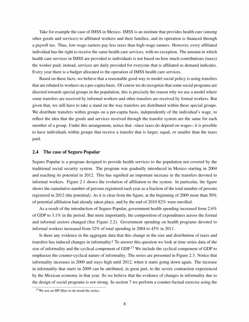
2.4 The case of Seguro Popular

Seguro Popular is a program designed to provide health services to the population not covered by the

traditional social security system. The program was gradually introduced in Mexico starting in 2004

and reaching its potential in 2012. This has signified an important increase in the transfers devoted to

informal workers. Figure 2.1 shows the evolution of affiliation to the system. In particular, the figure

shows the cumulative number of persons registered each year as a fraction of the total number of persons

registered in 2012 (the potential). As it is clear from the figure, at the beginning of 2009 more than 50%

of potential affiliation had already taken place, and by the end of 2010 82% were enrolled.

As a result of the introduction of Seguro Popular, government health spending increased from 2.6%

of GDP to 3.1% in the period. But more importantly, the composition of expenditures across the formal

and informal sectors changed (See Figure 2.2). Government spending on health programs devoted to

informal workers increased from 32% of total spending in 2004 to 45% in 2011.

Is there any evidence in the aggregate data that this change in the size and distribution of taxes and

transfers has induced changes in informality? To answer this question we look at time series data of the

size of informality and the cyclical component of GDP.13 We include the cyclical component of GDP to

emphasize the counter-cyclical nature of informality. The series are presented in Figure 2.3. Notice that

informality increases in 2009 and stays high until 2012, when it starts going down again. The increase

in informality that starts in 2009 can be attributed, in great part, to the severe contraction experienced

by the Mexican economy in that year. So we believe that the evidence of changes in informality due to

the design of social programs is not strong. In section 7 we perform a counter-factual exercise using the

13We use an HP-filter to de-trend the series.

8

Figure 2.1: Affiliation to Seguro Popular

2000 2002 2004 2006 2008 2010 20120

0.1

0.2

0.3

0.4

0.5

0.6

0.7

0.8

0.9

1

Afil

iatio

n to

SP

/ P

oten

tial A

filia

tion

Source: Sistema de Protección Social en Salud. Informe de Resultados 2012.

Figure 2.2: Informal/Formal Government Health Expenditure Ratio

2000 2002 2004 2006 2008 2010 20120.45

0.5

0.55

0.6

0.65

0.7

0.75

0.8

0.85

0.9

Info

rmal

/For

mal

Gov

ernm

ent H

ealth

Exp

endi

ture

Rat

io

Data source: Ministry of Health .

9

Figure 2.3: Evolution of informality among employees

0.47

0.48

0.49

0.50

0.51

0.52

0.53

0.54

-0.08

-0.06

-0.04

-0.02

0

0.02

0.04

20

00

q2

20

01

q2

20

02

q2

20

03

q2

20

04

q2

20

05

q2

20

06

q2

20

07

q2

20

08

q2

20

09

q2

20

10

q2

20

11

q2

20

12

q2

20

13

q2

GDP gap Informal share (right axis) Informal share trend (right axis)

Source: Own calculation using ENE, ENOE and National Accounts.

model described in Section 4 and show that our model predicts a small increase on informality due to the

introduction of Seguro Popular. This is consistent with the evidence found elsewhere14.

14See footnote 2

10

3 A basic model of informality with homogenous workers

In this section we would like to review the standard results of two-sector models with homogenous

workers and no labor market frictions (i.e. no unemployment). This will be useful to later compare

these results against the ones from our framework with heterogeneous workers and frictions. These

models typically assume an exogenously given supply of labor, and a demand curve for each type of

worker, formal and informal (e.g. Maloney (2004); Fields (1990, 2004); and Levy, 2008). One can

think of two representative firms, one formal and one informal that lead to these demands through profit

maximization.

On the worker’s side, it is assumed that there is a continuum of identical workers with mass 1, and

each worker can freely choose to work either as a formal or as an informal worker. If formal, the worker

receives the wage wF , if informal, the worker obtains wage wI . We will consider the inclusion of taxes

and transfers in a second stage. Market clearing works in the following way: labor demand equals labor

supply for each type of worker, and, in addition, the sum of formal workers plus informal workers has to

be equal to 1 (the total mass of workers).

Due to free mobility, in this economy wages must equalize:

wF = wI,

and given the absence of taxes or transfers, this also implies that the marginal cost of a formal worker

is equal to the marginal cost of an informal worker. Figure 3.1 depicts the equilibrium for this simple

economy. As shown by Fig. 3.1, firms demand labor until the marginal benefit of an extra worker is equal

to its marginal costs. The total amount of formal labor demanded is given by the intersection of curve

DF and marginal cost wF . This is measured in the x-axis from left to right by the distance OF . Similarly,

the quantity demanded of informal labor is given by the intersection of DI and wI , and is measured in the

x-axis from right to left by the distance PF . Notice that the sum of formal workers and informal workers

is equal to the distance OP which measures the total amount of labor available in the economy. Thus, in

these models, the size of the informal sector is “positive” even in the absence of taxes and transfers. For

later reference, we will refer to this equilibrium as the “undistorted” equilibrium.

Now consider an economy with taxes. In particular assume that the formal workers have to pay a

fixed rate τ > 0 of their income. In this case, due to free mobility, it is the case that:

(1− τ)wF = wI. (3.1)

What must be equalized is net earnings in order to eliminate arbitrage opportunities. However, from the

perspective of the firms, marginal costs are still given by:

wF : MC f ormal worker

wI : MC in f ormal worker (3.2)

Thus, a labor tax introduces a wedge between the marginal cost of formal labor and the marginal cost

11

Figure 3.1: Equilibrium in a two-sector model with homogenous workers

of informal labor, in particular: wF > wI . This wedge affects the equilibrium by increasing the share of

informal labor as depicted in Figure 3.1 by the variables with an apostrophe. As shown by Fig. 3.1, the

intersection of DF and w′F is at point B, which implies a smaller formal sector measured by OF ′ and a

larger informal sector PF ′.

Finally, consider an economy with taxes and transfers. Assume that τ > 0 as before, and that addi-

tionally, formal workers get a lump-sum transferT > 0. Again, due to free mobility, net earnings equalize

to eliminate arbitrage opportunities, and it must be that:

(1− τ)wF +T = wI

⇐⇒ wF − τwF +T = wI (3.3)

Now, to understand the implications of the interaction of these two policies on the marginal costs faced

by firms, lets consider the next three general cases:

a)T = τwF ,

b)T < τwF , and

c)T > τwF .

Case (a) corresponds to a situation when the workers get back all what they paid in taxes. In this case,

marginal costs of formal and informal workers equalize: wF − τwF + T = wI ⇔ wF = wI. The first

equality follows from the free mobility condition, while the second one follows from the equation (a)

above. Therefore, when the formal workers are given back their taxes, the equilibrium is the same as in

the undistorted case.

Case (b) T < τwF corresponds to the situation when the workers do not get back the total proceeds

of their taxes. In this case, a wedge between the marginal cost of formal workers and that of informal

workers is present, in particular: wF > wI . The equilibrium for this case is similar to the case when we

12

only had a tax and no transfer and the informal sector increases. In fact, T = 0, can be seen as an extreme

case of (b).

The opposite happens in case (c), T > τwF , where the workers get more than what they paid in taxes.

A wedge between the marginal cost of a formal worker and an informal one is introduced again, but

in this case wF < wI and, as a consequence, the formal sector increases. This situation is depicted in

Figure 3.1 with the variables labeled with two apostrophes. The marginal cost of a formal worker is now

intersected with DF at point C in the graph. This implies that the formal sector is given by the distance

OF ′′.

Given our assumption of homogenous workers, cases (b) and (c), correspond to situations where

the budget of the government is not balanced. However, when there are heterogeneous workers, cross-

subsidies between high-income and low-income workers, allow for the possibility to have all three cases

above simultaneously, and, at the same time, to have a balanced budget in equilibrium. In our model

below, we will have workers that receive more than what they paid in taxes, workers that receive less

than what they paid in taxes, and workers that receive the same than what they paid. We will argue that the

marginal workers, that is, those workers that are indifferent between being formal or informal, receive

more transfers than what they pay in taxes (case c above, T > τwF ). Consequently, a more generous

system will increase transfers proportionally more than taxes for these marginal workers, which will

result in an increase of the formal sector.

4 Model with frictions and (ex-post) heterogeneous workers

To study the effects of the structure of taxes and transfers in Mexico, we build a search model that

features a formal sector, an informal sector, and unemployment. The economy is populated with a

continuum of risk-neutral workers that discount consumption streams at a rate β . Workers are ex-ante

identical but face random draws from two different, and independent distributions of wage offers. GF

is the distribution of wage offers in the formal sector and GI is the distribution of wage offers in the

informal sector. The individual state variables are employment status (formal, informal), unemployment

status (formal or informal) and current wage (wF or wI).15 We refer to unemployed individuals that

previously had a formal job as “formal unemployed”, and we use the term “informal unemployed” in an

analogous way. Employed workers face an exogenous sector specific separation probability, λi where

i ∈ F, I. As we abstract from on the job search, observed transitions in any direction between formal

and informal employment include a period of unemployment.

The structure of taxes and transfers in the model is as follow. Workers employed in the formal sector

pay a proportional tax on wages τwF whereas those employed in the informal sector do not pay taxes.

Tax revenue is the sum of all taxes paid by formal workers. A fraction θ of the tax proceeds is transferred

to formal workers and the remaining fraction (1−θ) is transferred to informal workers. These transfers

are on a per capita basis: a formal worker receives TF , while an informal worker receives TI . We think

of these per-cápita transfers as the value of all cash and in-kind benefits accrued to workers. These

15We abstract from sub-index t, since we will be focusing on the steady state.

13

might include health services, retirement benefits, unemployment insurance, and other social security

and social protection benefits.

Every period, unemployed workers get a draw from both formal and informal sector wage distribu-

tions with independent probabilities qi where i ∈ F, I. They must choose whether they remain unem-

ployed or accept any of the offers at hand. Next, we write down Bellman Equations that characterize the

decision of workers and lay out an equilibrium definition. For that we need to characterize the steady

state equilibrium levels of employment in the formal and informal sectors, unemployment, and the steady

state distributions of accepted wage offers in both sectors.

4.1 Value functions

The decision problem of an individual is characterized by four Bellman Equations: the value of being

employed in the formal sector with a wage wF , VF(wF); the value of being employed in the informal

sector with a wage wI , VI(wI), and the values of being formal or informal unemployed UF , and UI .

• Value of being employed in the formal sector:

VF(wF) = TF +(1− τ)wF +β [λFUF +(1−λF)VF(wF)] (4.1)

• Value of being employed in the informal sector:

VI(wI) = TI +wI +β [λIUI +(1−λI)VI(wI)] (4.2)

• Value of being unemployed after having a formal job:

UF = TF +β [qFqIE max

VF(w′F),VI(w′I),UF+qF(1−qI)E maxVF(w′F),UF...

+qI(1−qF)E maxVI(w′I),UF+(1−qF)(1−qI)UF ] (4.3)

• Value of being unemployed after having an informal job:

UI = TI +β [qFqIE max

VF(w′F),VI(w′I),UI+qF(1−qI)E maxVF(w′F),UI...

+qI(1−qF)E maxVI(w′I),UI+(1−qF)(1−qI)UI] (4.4)

The value functions define reservation wages in equilibrium. These will be critical in determining equi-

librium flows among both types of employment and both types of unemployment. Note that we will have

four different reservation wages: a reservation wage of an formal unemployed worker facing an offer

from the formal sector (wRFF ); a reservation wage of an formal unemployed worker facing an offer from

the informal sector (wRFI); a reservation wage of an informal unemployed worker facing an offer from the

formal sector (wRIF ,); and a reservation wage of an informal unemployed worker facing an offer from the

informal sector (wRII). To define these reservation wages we use 4.1 - 4.4, above.

14

VF(wR

FF)

= UF (4.5)

VI(wR

II)

= UI (4.6)

VF(wR

IF)

= UI (4.7)

VI(wR

FI)

= UF (4.8)

4.2 Steady State Employment, Unemployment and Wage Distributions

With the reservation wages we are able to define the steady state levels of employment and unemploy-

ment and the stationary wage distributions in the formal and informal sectors. Let eFt be the employment

in the formal sector at date t. Similarly, we can define eIt , uF

t , and uIt . The evolution of these variables is

driven by reservation wages, distributions of wage offers, and separation and wage drawing probabilities.

The evolution of these aggregate variables is defined by the following set of difference equations:

eF,t+1 = (1−λF)eF,t +qF(1−qI) [Prob(VF >UF)uF,t +Prob(VF >UI)uI,t ]

+ qFqI[Prob(VF >UF)Prob(VI >UF)Prob(VF >VI)uF,t

+ Prob(VF >UI)Prob(VI >UI)Prob(VF >VI)uI,t

+ Prob(VF >UF)Prob(VI <UF)uF,t +Prob(VF >UI)Prob(VI <UI)uI,t ]

eI,t+1 = (1−λI)eI,t +qI(1−qF) [Prob(VI >UF)uF,t +Prob(VI >UI)uI,t ]

+ qFqI[Prob(VF >UF))Prob(VI >UF))Prob(VI >VF)uF,t

+ Prob(VF >UI))Prob(VI >UI))Prob(VI >VF)uI,t

+ Prob(VF <UF)Prob(VI >UF)uF,t +Prob(VF <UI)Prob(VI >UI)uI,t ]

uF,t+1 = [(1−qF)(1−qI)+qF(1−qI)Prob(VF ≤UF)+qI(1−qF)Prob(VI ≤UF)

+ qFqIProb(VF ≤UF)Prob(VI ≤UF)]uF,t +λFeF,t .

1 = eF,t+1 + eI,t+1 +uF,t+1 +uI,t+1

Consider the first equation that defines employment in the formal sector next period. The first com-

ponent is the mass of workers whom did not loose their formal employment. The second component are

those workers that receive an offer from the formal sector, do not receive an offer fro the informal sector,

and accept the offer. Finally, we have unemployed workers that get offers from both sectors, but the for-

mal sector offer dominates. The second equation follows a similar logic for the informal workers. The

third equation describes the evolution of unemployment. The unemployment rate tomorrow is the sum of

those workers that do not get offers, plus those that get offers but reject them, plus an inflow of workers

that lost their employment in period t. This system of equations define a steady state for employment

and unemployment distributions. Key to define steady state employment and unemployment by sector

in equilibrium are the probabilities that compare different offers. In the calibration we will assume log-

15

normality of distributions from where workers draw offers, which will facilitate the computation of these

probabilities. As wage draws from formal and informal sector belong to different log-normal distribu-

tions there is not an analytic solution to Prob(VF >VI). We log-linearize each value function around its

respective mean wage.

VF(wF)|µF −→ N

((1− τ)eµF +βλFUF

1−β (1−λF),

[(1− τ)eµF

1−β (1−λF)

]2

σ2F

)

VI(wI)|µI −→ N

(eµI +βλIUI

1−β (1−λI),

[eµI

1−β (1−λI)

]2

σ2I

)

VF(wF)|µF −VI(wI)|µI −→ N((1− τ)eµF +βλFUF

1−β (1−λF)− eµI +βλIUI

1−β (1−λI),[

(1− τ)eµF

1−β (1−λF)

]2

σ2F +

[eµI

1−β (1−λI)

]2

σ2I

)

We need to define the equilibrium distribution of accepted wage offers. These can be computed from

the primitive distribution of wage offers and individual behavior. Let ΓF,t and ΓI,t be the equilibrium

distributions of accepted wage offers on each sector:

ΓF,t+1(wF) = (1−λF)ΓF,t(wF)+qFqIgF(wF)[I(wF > wR

FF)Pr(VI >UF)

Pr(VF(wF)>VI)uF,t + I(wF > wRIF)Pr(VI >UI)Pr(VF(wF)>VI)uI,t

+ I(wF > wRFF)Pr(VI <UF)uF,t + I(wF > wR

IF)Pr(VF(wF)>VI)uI,t]

+ qF(1−qI)gF(wF)[I(wF > wR

F)ut]

ΓI,t+1(wI) = (1−λI)ΓI,t(wI)+qFqIgI(wI)[I(wI > wR

FI)Pr(VI >UF)

Pr(VI(wI)>VF)uF,t + I(wI > wRII)Pr(VF >UI)Pr(VI(wI)>VF)uI,t

+ I(wI > wRFI)Pr(VF <UF)uF,t + I(wI > wR

II)Pr(VF <UI)uI,t]

+ qI(1−qF)gI(wI)[I(wI > wR

FI)uF,t + I(wI > wRII)uI,t

]Where I(w > wR) is an indicator function equal to 1 if w > wR, and zero otherwise. Each of the equa-

tions above, can be used to find a steady state measure of accepted wage offers: ΓF and ΓI , respectively.

Since we normalized the measure of workers in the economy to one, this implies that´

dΓi(wi) = ei

where i ∈ F, I.

16

4.3 The tax and transfers system

The transfer system is defined in the steady state equilibrium. First, total resources collected by the

government are given by:

Ω = τ

ˆwFdΓF(wF).

θΩ is transferred to formal workers and the rest to informal workers. In turn, per-cápita transfers are

defined as:

TF = θΩ/(eF +uF) = θΩ/(

ˆdΓF(wF)+uF),

TI = (1−θ)Ω/(eI +uI) = (1−θ)Ω/(

ˆdΓi(wi)+uI).

5 Equilibrium characterization

The goal in this section is to describe characteristics of the equilibrium that are important for our main

results. We are particularly interested in the way workers react to changes in taxes and transfers. For di-

dactic purposes we will start with an analysis of what happens when the distribution of transfers changes;

then, we will consider the effects of an increase in taxes.

5.1 A shift of transfers towards formal individuals, increases the formal sector.

Consider the effects on the decisions of marginal workers when faced with changes in the distribution

of transfers, θ . Consider an increase in θ from θ0 to θ1, and focus on a formal unemployed individual.

The problem faced by this individual can be summarized in Figure 5.1. When θ = θ0, the reservation

wage equals wR0FF , in contrast, when theta increases to θ1, the reservation wage falls to wR1

FF . The reason

behind this drop in the reservation wage is that, as transfers increase, the value of both, formal jobs

and formal unemployment increase, but the former increases more than the latter. The value of formal

jobs increases because these now receive more transfers (and taxes remain constant); similarly, the value

of formal unemployment increases because it takes into account the discounted future value of formal

jobs. However, the value of formal unemployment is additionally affected by a negative force because

it has to weigh the possibility of ending-up with an informal job in the future (see equation 4.3). Since

informal jobs now receive less transfers, these are less valuable, and this tends to reduce the value of

formal unemployment.

Figure 5.2 shows what happens to the reservation wage of an informal unemployed individual when

θ increases. In this case, the reservation wage increases, because the value of an informal job is reduced

more than proportionally with respect to the value of informal unemployment. The reason for this is

similar than before, the value of informal unemployment has to take into account the possibility of

switching to a formal job next period. So, the drop in UI is not as large as the drop in VI .

17

Figure 5.1: Effects of an increase in θ on formal unemployed individuals.

Figure 5.2: Effects of an increase in θ on informal unemployed individuals.

18

Figure 5.3: Effects of a tax increase with no transfers on the value of a formal job.

5.2 Higher taxes do not necessarily imply higher informality

Now, lets analyze the mechanics of the model when taxes increase. To gain intuition, consider first

the case when θ = 0, that is, when no transfers are given to formal individuals. Focus on a formal

unemployed worker. The decision problem of this worker is summarized in Figure 5.3. Originally, taxes

are at τ0, thus, the value function is depicted by the solid line as an increasing function of the wage.

As Fig. 5.3 shows, the worker accepts the offer if wF > wR0FF (because VF > UF ) and rejects otherwise.

The effect of an increase in taxes from τ0 to τ1 is shown in Fig. 5.3 by the dashed line. Since (1− τ)

multiplies the wage in equation 4.1, the effect of an increase in taxes is to reduce the value of being

formal for every possible wage. Notice that the reduction in the value function is larger for high wage

earners than for low wage earners, which is a consequence of the proportionality of the tax. In sum,

this implies that the reservation wage increases to wR1FF , and, as a result, less workers decide to become

formal.16 In this case, higher taxes bring a decrease in formality, in accordance to popular beliefs.

Now consider what happens when transfers to formal workers are positive (θ > 0), for didactic

purposes focus on the case when θ = 1. In this case, an increase in taxes will come associated with an

increase in transfers to formal workers. However, due to the fact that transfers are given on a per-cápita

basis and taxes are proportional to the wage, transfers will increase more than taxes for workers with a

low wage, and will increase less than taxes for workers with a high wage. In other words, high-wage

earners will subsidize low-wage earners through the tax and transfer system. The effect of increasing

taxes in this context is depicted in Figure 5.4. The dashed line lies below the solid line for high wages,

while it lies above the solid line for low wages; since the original reservation wage is low, this implies

that the formal sector becomes more attractive for the marginal worker. Consequently, the reservation

wage goes down, and more unemployed workers decide to go into the formal sector. 17

16To be precise, the value of formal unemployment would also shift in response to the tax change, but the shift will besmall. The reason for this is that the value of formal unemployment takes into account the possibility of ending-up accepting aninformal job offer. In this particular example, the value of informal jobs after the tax change is higher because they are gettingall the extra revenue from the increase in taxes (1−θ = 1).

17Notice that the value of formal unemployment will also change, but this change will be small due to similar reasons as in

19

Figure 5.4: Effects of a tax increase with all transfers to formal workers.

In summary, this analysis suggests that the formal sector can be increased if more transfers are given

to formal workers, even if the extra resources are obtained through higher taxes. This result holds as

long as the value of θ ∈ 0,1 remains sufficiently high. We believe this is an important result because

it contrasts with the common idea that higher taxes imply, automatically, more informality.

the previous footnote.

20

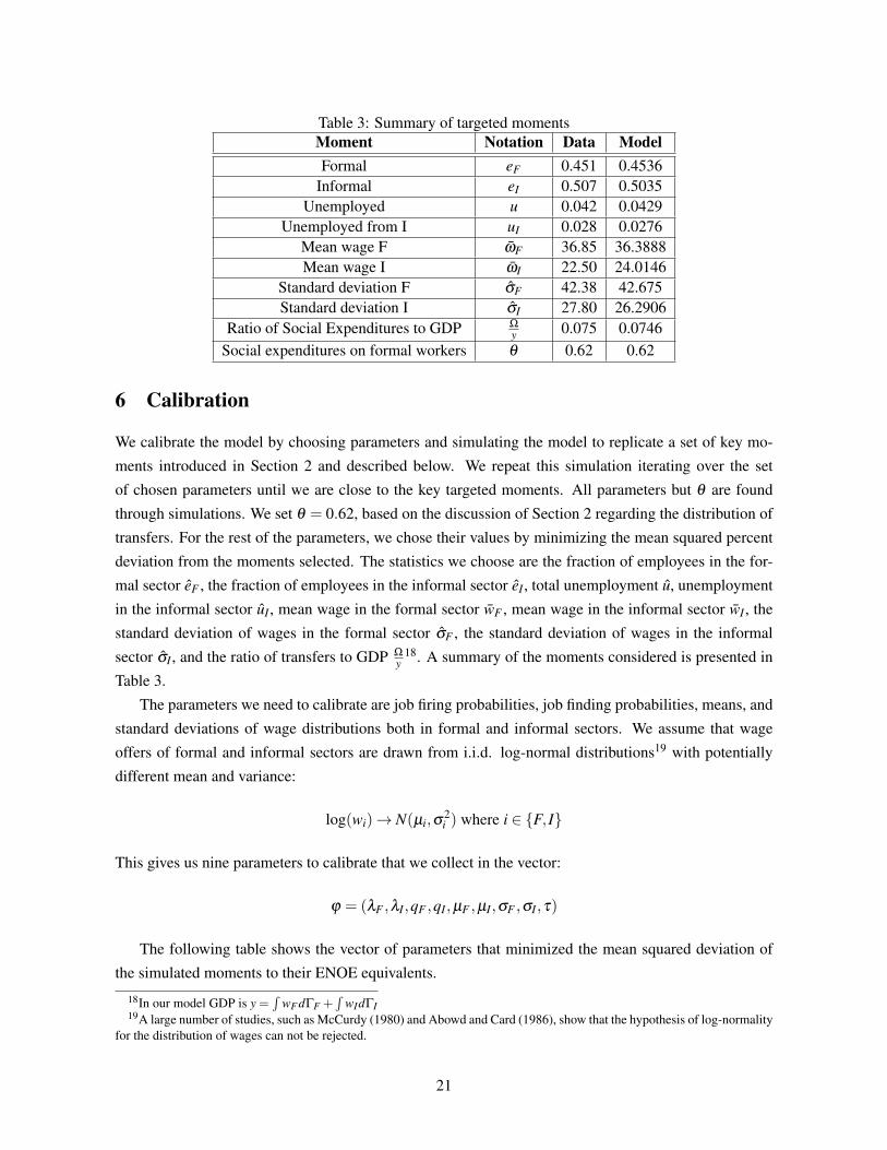
Table 3: Summary of targeted momentsMoment Notation Data ModelFormal eF 0.451 0.4536

Informal eI 0.507 0.5035Unemployed u 0.042 0.0429

Unemployed from I uI 0.028 0.0276Mean wage F ωF 36.85 36.3888Mean wage I ωI 22.50 24.0146

Standard deviation F σF 42.38 42.675Standard deviation I σI 27.80 26.2906

Ratio of Social Expenditures to GDP Ω

y 0.075 0.0746Social expenditures on formal workers θ 0.62 0.62

6 Calibration

We calibrate the model by choosing parameters and simulating the model to replicate a set of key mo-

ments introduced in Section 2 and described below. We repeat this simulation iterating over the set

of chosen parameters until we are close to the key targeted moments. All parameters but θ are found

through simulations. We set θ = 0.62, based on the discussion of Section 2 regarding the distribution of

transfers. For the rest of the parameters, we chose their values by minimizing the mean squared percent

deviation from the moments selected. The statistics we choose are the fraction of employees in the for-

mal sector eF , the fraction of employees in the informal sector eI , total unemployment u, unemployment

in the informal sector uI , mean wage in the formal sector wF , mean wage in the informal sector wI , the

standard deviation of wages in the formal sector σF , the standard deviation of wages in the informal

sector σI , and the ratio of transfers to GDP Ω

y18. A summary of the moments considered is presented in

Table 3.

The parameters we need to calibrate are job firing probabilities, job finding probabilities, means, and

standard deviations of wage distributions both in formal and informal sectors. We assume that wage

offers of formal and informal sectors are drawn from i.i.d. log-normal distributions19 with potentially

different mean and variance:

log(wi)→ N(µi,σ2i ) where i ∈ F, I

This gives us nine parameters to calibrate that we collect in the vector:

ϕ = (λF ,λI,qF ,qI,µF ,µI,σF ,σI,τ)

The following table shows the vector of parameters that minimized the mean squared deviation of

the simulated moments to their ENOE equivalents.

18In our model GDP is y =´

wF dΓF +´

wIdΓI19A large number of studies, such as McCurdy (1980) and Abowd and Card (1986), show that the hypothesis of log-normality

for the distribution of wages can not be rejected.

21

Table 4: Calibrated ParametersλF λI qF qI µF µI σF σI Ω

0.0238 0.0395 0.3157 0.9092 2.946 2.2681 0.9919 1.0227 4.505

The firing probability in the formal sector is smaller than in the informal sector. This is an important

feature in our model and it is related with the assumption of two different unemployment states. When

we consider two different unemployment states, we also ask in the calibration to match the stocks of

each type of unemployment. Since the stock of formal unemployment is substantially lower than the

stock of informal unemployment, a lower firing probability in the formal sector is needed. Furthermore,

the per-capita transfer received by the formal unemployed is higher than the per-capita transfer received

by the informal unemployed which tends to increase duration. A higher duration would tend to increase

formal unemployment, this is offset with a low firing probability in the formal sector.

This feature is consistent with the common idea that being unemployed after having a formal sector

job leaves the worker in a much better position than being unemployed after having an informal job. The

source of this idea is that the formal sector in Mexico is subject to high severance payments. We do

not model explicitly severance payments, but we believe that the current specification is rich enough to

capture the mechanics behind this common idea.

Similarly, job finding probabilities are smaller in the formal sector than in the informal sector, which

is also consistent with the idea that the informal sector is more dynamic as is not subject to labor market

regulations. Finally, the tax consistent with a revenue of 7.5% of GDP is τ = 0.2729, which lies within a

reasonable range. We compare moments induced by these parameters against those in the data in Table

3.

The model provides a good match of employment and unemployment and it captures very well the

first two moments of the observed distribution of wages.

7 Results

We would like to organize the discussion analyzing two general policy changes: 1) changes in the size of

transfers (i.e. higher taxes), given a constant distribution; and 2) changes in the distribution of transfers

given size. Of course, we would also like to analyze policy changes that involve a combination of the

above two cases.

7.1 Changes in the distribution of transfers

Consider first changes in the distribution of transfers, this is presented in Table 5. The benchmark values

for the size of the informal sector, the formal sector, general unemployment, and formal unemployment

are shown in the column in bold (θ = .62). Notice also, that in this table the size of transfers is kept

constant, which corresponds to a value of τ in our benchmark of 0.2729. When the fraction of resources

devoted to formal workers increases to θ = 1, the size of the informal sector decreases to 0.4288; and

there is a corresponding increase in the size of the formal sector, this corresponds to the case when all

22

Table 5: Effects of changes in the distribution of transfers, given size.Panel a

θ

0 .25 .50 .62 1eI 0.7108 0.6096 0.5345 0.5035 0.4288eF 0.2435 0.3466 0.4226 0.4536 0.527

u = uF +uI 0.0458 0.0437 0.0429 0.0429 0.0442uF 0.0077 0.0112 0.014 0.0152 0.0191

Panel bwR

FF 13.9765 8.2773 4.948 3.6408 0wR

II 4.9846 5.4061 6.0197 6.3654 7.8812wR

IF 14.3051 8.3086 4.7519 3.3263 0wR

FI 4.6826 5.3862 6.2247 6.6819 8.5962ωF 50.5172 42.0108 37.797 36.3888 33.8177ωI 21.4012 22.3066 23.416 24.0146 26.4573σF 50.8386 45.4272 43.2986 42.675 41.5513σI 24.7335 25.3316 25.9631 26.2906 27.5599

the tax revenue is given to formal workers. In contrast, when the tax revenue is given only to informal

workers (θ = 0), informality goes up to 0.7108. This shows that the way transfers are distributed across

formal and informal workers is a relevant force that determines the size of the informal sector. (see

Figures 5.1 and 5.2).

Also of interest is the response of unemployment to the increase in θ . As the value of transfers to

formal workers increases, formal unemployment increases. This is explained by two effects, first, the

increase in formality increases the number of people that can potentially be formal unemployed; second,

since transfers also increase for the formal unemployed this also increases the value of formal unem-

ployment. Notice however, that general unemployment is almost unchanged, which is consistent with an

offsetting reduction of informal unemployment. To see why, notice that when θ increases, there is less in-

formality and less transfers are given to informal unemployed. General unemployment is barely affected

because the changes in θ do not affect the distribution of transfers across employment/unemployment

status in an important way.

It is also interesting to look at the way reservation wages respond to changes in θ in order to fully

understand the mechanics of the model. Notice that, as θ increases, the reservation wage of a formal

unemployed individual with an offer from the formal sector (and no offer from the informal sector), wRFF ,

is reduced. This means that more formal jobs are accepted. Similarly, the reservation wage of an informal

unemployed with a formal offer in hand is reduced, in fact, when θ = 1, practically any formal job offer

is accepted (wRIF = 0). The reduction on the reservation wage occurs despite the fact that the value of

formal unemployment is higher when θ increases. Nonetheless, the value of a formal job increases more

than the value of formal unemployment, which reduces the reservation wage (see Figure 5.1).

In contrast, the reservation wage of an informal offer increases when θ goes up. This reflects the

fact that informal jobs become less attractive as less transfers are given to these individuals (see Figure

23

Table 6: Effects of changes in size and distribution of transfers on the size of the informal sectorθ

0 .25 .50 .62 1

τ/τ0

.8 0.6657 0.5934 0.5333 0.5074 0.4371

.9 0.6869 0.6015 0.534 0.5054 0.43241 0.7108 0.6096 0.5345 0.5035 0.4288

1.1 0.7391 0.6176 0.5349 0.5020 0.42531.2 0.7808 0.6256 0.5354 0.5009 0.4219

5.2). Consequently, less informal jobs are accepted, and the size of the informal sector is reduced.

Furthermore, a larger amount of formal jobs with low wages are accepted and thus the mean wage in the

formal sector is reduced. The opposite happens with the mean wage of informal jobs.

7.2 Changes in the generosity of transfers (the tax rate)

Consider now changes in the size of transfers, given the current distribution. What is the effect on the

size of the informal sector of increasing taxes in 20%? Table 6 shows this in the column in bold. The

benchmark value of τ is (0.2729), and we present the effects of increasing and reducing this parameter

in 10 and 20%. This implies that the value of τ ranges between 22% to 33%.

In response to a 20% increase in τ , informality would barely change, in fact it decreases by less than

half of a percentage point (from 0.5035 to 0.5009). This sign of this change is opposite to the popular

idea that more taxes induce higher informality. However, we would like to stress that in the present

model, the effect of tax increases depends heavily on the parameter θ . If all tax revenue is given back to

formal workers (θ = 1), a tax hike actually decreases informality as discussed before (see Figure 5.4).

This can be confirmed in the last column of Table 6: when the tax rate increases, informality goes down

from 0.4288 to 0.4219. In contrast, when all tax revenue is transferred to informal workers (i.e. θ = 0),

the result of an increase in taxes is what most people would expect: a severe increase of informality (see

Figure 5.3).

Above all, the most important result derived from table 6 is that informality is pretty inelastic to

changes in τ for an important range of values of θ . To put this into perspective, notice that Tab. 6

considers changes in the tax rate in a range of 10 percentage points (from 22% to 33%), and only when

θ = 0, the range of variation of informality in response to changes in τ is more than 10 percentage

points. However, for values above θ = .25, the range of variation of informality in the table is less

than 3 percentage points. In sum, the results in this table imply that the elasticity of informality to

realistic changes in taxes and transfers is small. This is confirmed next, when we study the effects of the

introduction of Seguro Popular.

7.3 Effects of Seguro Popular

In this section we analyze the effect of changes in taxes and transfers associated with the introduction

of Seguro Popular (SP). We interpret the calibrated parameters above as representing the situation after

24

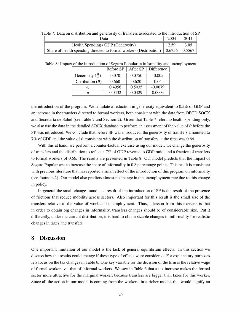
Table 7: Data on distribution and generosity of transfers associated to the introduction of SPData 2004 2011

Health Spending / GDP (Generosity) 2.59 3.05Share of health spending directed to formal workers (Distribution) 0.6756 0.5567

Table 8: Impact of the introduction of Seguro Popular in informality and unemploymentBefore SP After SP Difference

Generosity ( Ω

y ) 0.070 0.0750 -0.005Distribution (θ ) 0.660 0.620 0.04

eI 0.4956 0.5035 -0.0079u 0.0432 0.0429 0.0003

the introduction of the program. We simulate a reduction in generosity equivalent to 0.5% of GDP and

an increase in the transfers directed to formal workers, both consistent with the data from OECD SOCX

and Secretaría de Salud (see Table 7 and Section 2). Given that Table 7 refers to health spending only,

we also use the data in the detailed SOCX database to perform an assessment of the value of θ before the

SP was introduced. We conclude that before SP was introduced, the generosity of transfers amounted to

7% of GDP and the value of θ consistent with the distribution of transfers at the time was 0.66.

With this at hand, we perform a counter-factual exercise using our model: we change the generosity

of transfers and the distribution to reflect a 7% of GDP revenue to GDP ratio, and a fraction of transfers

to formal workers of 0.66. The results are presented in Table 8. Our model predicts that the impact of

Seguro Popular was to increase the share of informality in 0.8 percentage points. This result is consistent

with previous literature that has reported a small effect of the introduction of this program on informality

(see footnote 2). Our model also predicts almost no change in the unemployment rate due to this change

in policy.

In general the small change found as a result of the introduction of SP is the result of the presence

of frictions that reduce mobility across sectors. Also important for this result is the small size of the

transfers relative to the value of work and unemployment. Thus, a lesson from this exercise is that

in order to obtain big changes in informality, transfers changes should be of considerable size. Put it

differently, under the current distribution, it is hard to obtain sizable changes in informality for realistic

changes in taxes and transfers.

8 Discussion

One important limitation of our model is the lack of general equilibrium effects. In this section we

discuss how the results could change if these type of effects were considered. For explanatory purposes

lets focus on the tax changes in Table 6. One key variable for the decision of the firm is the relative wage

of formal workers vs. that of informal workers. We saw in Table 6 that a tax increase makes the formal

sector more attractive for the marginal worker, because transfers are bigger than taxes for this worker.

Since all the action in our model is coming from the workers, in a richer model, this would signify an

25

increase in the supply of formal workers and a decrease in the supply of informal workers. An increase

in the supply of formal workers would tend to push formal wages down relative to the informal wages,

in order to keep demand in line with supply. This effect would reduce the value of formal sector jobs,

and increase the value of informal jobs. Thus, general equilibrium introduces a feedback effect that go

in the opposite direction of our current results.

How much would formal sector wages go down after an increase in taxes? Would it be enough to end

up reducing the size of the formal sector? The answer to this is related to how substitutable are formal and

informal workers from the point of view of the firms. In models where there is an occupational choice

with formal and informal entrepreneurs, the answers to these questions are related to how the marginal

entrepreneurs are affected with changes in relative wages. Now consider a change in the distribution of

transfers in favor of formal workers (see Table 5). In this case, the supply of formal workers will also

increase, and this will push wages down, which will reduce the value of formal jobs. The extent of this

“feedback” effect remains a quantitative questions that we leave for future research.

9 Conclusion

In this paper we have used a search frictions model to study the elasticity of informality to changes in

social policy transfers. In our model formal jobs are “better” than informal jobs because they are tied

to larger transfers, and are less risky. On the other hand formal jobs are harder to get. Thus, workers

optimally decide to accept informal jobs because these arrive more frequently.

In contrast to the basic model of informality, we do not rely on the assumption of partial valuation

of benefits to obtain a non-zero elasticity of informality to taxes and transfers. Instead we use a model

where workers are heterogeneous in the wages they accept, and thus, the tax and transfer system allows

for a cross subsidy from high-wage earners to low-wage earners. In this model, workers that receive

a transfer that is larger than the taxes paid coexist with workers that receive transfers that are equal or

smaller than the taxes paid. The sign and magnitude of the elasticity of informality to changes in taxes

and transfers greatly depends on which of the two situations above is the one prevailing for the marginal

worker.

We calibrate the model for Mexico, and perform counter-factuals. Given that 62% of social expendi-

ture is given to formal workers, we find that the elasticity of informality to tax changes, given distribution

is small. The reason is that the marginal worker faces two opposing forces: higher taxes that reduce the

value of a formal job, vs. higher transfers that increase the value of a formal job.

We use our model to study the effects on informality of the recently introduced Seguro Popular, and

we find that the effects are quite small in line with the empirical literature using micro-data. Our model

also offers an alternative way to rationalize the empirical evidence found in Almeida and Carneiro (2012),

where an increase in taxes (due to an increase in enforcement) is associated with more formalization.

26

References

ABOWD, J. M. AND D. CARD (1986): “On the covariance structure of earnings and hours changes,”

Econometrica, 57.

ALBRECHT, J., L. NAVARRO, AND S. VROMAN (2009): “The Effects of Labour Market Policies in an

Economy with an Informal Sector*,” The Economic Journal.

ALMEIDA, R. AND P. CARNEIRO (2012): “Enforcement of Labor Regulation and Informality,” Ameri-

can Economic Journal: Applied Economics, 4, 64–89.

AZUARA, O. AND I. MARINESCU (2013): “Informality and the expansion of social protection programs:

Evidence from Mexico,” Journal of health economics.

BOSC, M. AND R. M. CAMPOS-VÁZQUEZ (2010): “The Trade-offs of Social Assistance Programs in

the Labor Market: The Case of the" seguro Popular" Program in Mexico,” .

BOSCH, M. AND J. ESTEBAN-PRETEL (2012): “Job creation and job destruction in the presence of

informal markets,” Journal of Development Economics, 98, 270–286.

CHANDRA, V. AND M. A. KHAN (1993): “Foreign investment in the presence of an informal sector,”

Economica.

DUVAL HERNÁNDEZ, R. AND R. SMITH RAMÍREZ (2011): “Informality and Seguro Popular under

Segmented Labor Markets,” .

EDWARDS, S. AND A. C. EDWARDS (2002): “Social Security Privatization Reform and Labor Markets,”

NBER WORKING PAPER SERIES.

ESTEBAN-PRETEL, J. AND S. KITAO (2013): “Labor Market Policies in a Dual Economy,” .

FIELDS, G. S. (1990): “Labour market modelling and the urban informal sector: theory and evidence,” .

——— (2004): “Dualism in the labor market: a perspective on the Lewis model after half a century,”

The Manchester School, 72, 724–735.

FUGAZZA, M. AND J. F. JACQUES (2004): “Labor market institutions, taxation and the underground

economy,” Journal of Public Economics.

KUGLER, A. D., M. KUGLER, AND NATIONAL BUREAU OF ECONOMIC RESEARCH (2008): “Labor

market effects of payroll taxes in developing countries,” .

LEVY, S. (2008): Good Intentions, Bad Outcomes, Social Policy, Informality, and Economic Growth in

Mexico, Brookings Institution Press.

LEWIS, W. A. (1954): “Economic Development with Unlimited Supplies of Labour,” The Manchester

School, 22, 139–191.

27

LOAYZA, N. V. (1994): “Labor regulations and the informal economy,” Policy Research Working Paper

Series.

MALONEY, W. F. (2004): “Informality Revisited,” World Development, 32, 1159–1178.

MCCURDY, T. E. (1980): “An Empirical Model of Labor Supply in a Life Cycle Setting,” The Journal

of Political Economy, 89, 1059–1085.

MEGHIR, C., R. NARITA, J.-M. ROBIN, NATIONAL BUREAU OF ECONOMIC RESEARCH, AND YALE

UNIVERSITY. ECONOMIC GROWTH CENTER (2012): “Wages and Informality in Developing Coun-

tries,” NBER WORKING PAPER SERIES.

PERRY, G., W. F. MALONEY, O. S. ARIAS, P. FAJNZYLBER, A. MASON, AND J. SAAVEDRA-

CHANDUVI (2007): “Informality: Exit and exclusion,” The World Bank.

SATCHI, M. AND J. TEMPLE (2009): “Labor markets and productivity in developing countries,” Review

of Economic Dynamics, 12, 183–204.

SUMMERS, L. H. (1989): “Some simple economics of mandated benefits,” The American Economic

Review.

ZENOU, Y. (2008): “Job search and mobility in developing countries. Theory and policy implications,”

Journal of Development Economics.

28