2014-01-28 Multibody Dynamics Course program tasks and the project report: Examination task 1: Rigid...
24
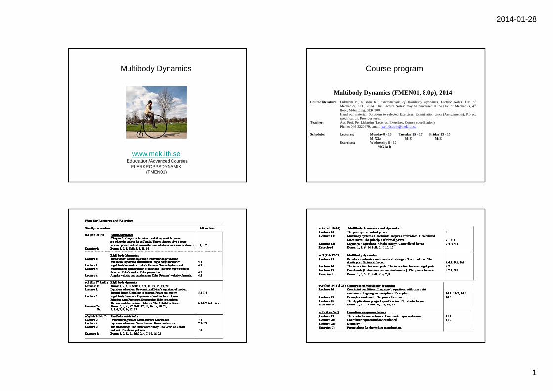
2014-01-28 1 Multibody Dynamics www.mek.lth.se Education/Advanced Courses FLERKROPPSDYNAMIK (FMEN01) Course program Multibody Dynamics (FMEN01, 8.0p), 2014 Course literature: Lidström P., Nilsson K.: Fundamentals of Multibody Dynamics, Lecture Notes. Div. of Mechanics, LTH, 2014. The ‘Lecture Notes’ may be purchased at the Div. of Mechanics, 4 th floor, M-building, SEK 300. Hand out material: Solutions to selected Exercises, Examination tasks (Assignments), Project specification. Previous tests. Teacher: Ass. Prof. Per Lidström (Lectures, Exercises, Course coordination) Phone: 046-2220479, email: [email protected] Schedule: Lectures: Monday 8 - 10 Tuesday 15 - 17 Friday 13 - 15 M:X2a M:E M:E Exercises: Wednesday 8 - 10 M:X1a-b
Transcript of 2014-01-28 Multibody Dynamics Course program tasks and the project report: Examination task 1: Rigid...
2014-01-28
1
Multibody Dynamics
www.mek.lth.seEducation/Advanced Courses
FLERKROPPSDYNAMIK (FMEN01)
Course program
Multibody Dynamics (FMEN01, 8.0p), 2014 Course literature: Lidström P., Nilsson K.: Fundamentals of Multibody Dynamics, Lecture Notes. Div. of
Mechanics, LTH, 2014. The ‘Lecture Notes’ may be purchased at the Div. of Mechanics, 4th floor, M-building, SEK 300. Hand out material: Solutions to selected Exercises, Examination tasks (Assignments), Project specification. Previous tests.
Teacher: Ass. Prof. Per Lidström (Lectures, Exercises, Course coordination) Phone: 046-2220479, email: [email protected] Schedule: Lectures: Monday 8 - 10 Tuesday 15 - 17 Friday 13 - 15 M:X2a M:E M:E
Exercises: Wednesday 8 - 10 M:X1a-b
2014-01-28
2
Course objectives
Course objectives: The objective of this course is to present the basic theoretical knowledge of the Foundations of Multibody Dynamics with applications to machine and structural dynamics. Course contents: 1) Topics presented at lectures and in the “Lecture Notes”. 2) Exercises. 3) Examination tasks 4) Application project The scope of the course is defined by the curriculum above and the lecture notes (Fundamentals of Multibody Dynamics, Lecture Notes). As a supplementary reading we may recommend Geradin M., Cardona A.; Flexible Multibody Dynamics, J. Wiley & Sons, 2001. The teaching consists of Lectures and Exercises: Lectures: Lectures will present the topics of the course in accordance with the curriculum presented above. Exercises: Recommended exercises worked out by the student will serve as a preparation for the Examination tasks. Solutions to selected problems will be distributed.
ExaminationExamination: The examination consists of two parts:
1. Hand in solutions to 3 examination tasks (assignments containing 2-4 problems each) and one Application project.
The examination tasks will be handed out starting by w.2. Last date for handing in solution to the examination tasks and the project report:
Examination task 1: Rigid body kinematics February 7th Examination task 2: Rigid and flexible body dynamics February 21st Examination task 3: Multibody dynamics Mars 3rd Application project (with Adams software) Mars 14th
2. Written examination containing five (5) tasks focusing on the theoretical parts of the course content.
A correctly solved task gives 3p (Total possible score 5x3p = 15p). The written examination: Thursday, Mars 13, 2013, 08:00 – 13:00, in room M:L1-L2. Credit requirements: Credit 3: Solutions to all examination tasks with 65% of the problems correctly solved. Passed project report. Written examination with 50% of the tasks correctly solved (7.5p). Credit 4: Solutions to all examination tasks with 75% of the problems correctly solved. Passed project report. Written examination with 67% of the tasks correctly solved (10p). Credit 5: Solutions to all examination tasks with 90% of the problems correctly solved. Passed project report. Written examination with 83% of the tasks correctly solved (12.5p).
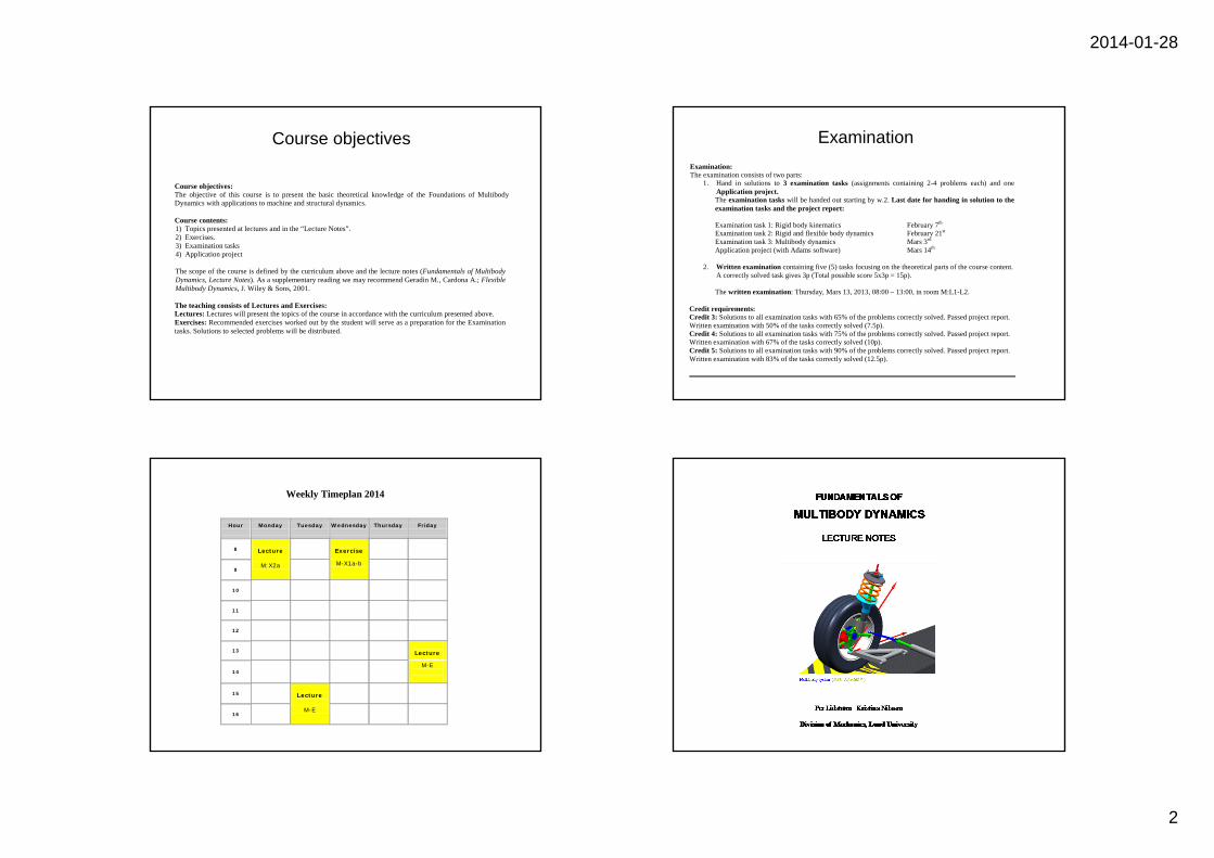
Weekly Timeplan 2014
Hour
Monday
Tuesday
Wednesday
Thursday
Friday
8
Lecture
M:X2a
Exercise
M-X1a-b
9
10
11
12
13
Lecture
14 M-E
15
Lecture
M-E
16

2014-01-28
3
CONTENTS
1. INTRODUCTION 1 2. BASIC NOTATIONS 12 3. PARTICLE DYNAMICS 13
3.1 One particle system 13 3.2 Many particle system 27
4. RIGID BODY KINEMATICS 36 4.1 The rigid body transplacement 36 4.2 The Euler theorem 47 4.3 Mathematical representations of rotations 59 4.4 Velocity and acceleration 72
5. THE EQUATIONS OF MOTION 89 5.1 The Newton and Euler equations of motion 89 5.2 Balance laws of momentum and moment of momentum 94 5.3 The relative moment of momentum 99 5.4 Power and energy 100
6. RIGID BODY DYNAMICS 104 6.1 The equations of motion for the rigid body 104 6.2 The inertia tensor 109 6.3 Fixed axis rotation and bearing reactions 138 6.4 The Euler equations for a rigid body 143 6.5 Power, kinetic energy and stability 158 6.6 Solutions to the equations of motion: An introduction to the case of
7. THE DEFORMABLE BODY 172 7.1 Kinematics 172 7.2 Equations of motion 196 7.3 Power and energy 205 7.4 The elastic body 209
8. THE PRINCIPLE OF VIRTUAL POWER 217 8.1 The principle of virtual power in continuum mechanics 219
1. THE MULTIBODY 222 9.1 Multibody systems 222 9.2 Degrees of freedom and coordinates 224 9.3 Multibody kinematics 229 9.4 Lagrange’s equations 232 9.5 Constitutive assumptions and generalized internal forces 252
9.6 External forces 261 9.7 The interaction between parts 267 9.8 The Lagrangian and the Power theorem 295
10. CONSTRAINTS 300 10.1 Constraint conditions 300 10.2 Lagrange’s equations with constraint conditions 305 10.3 The Power Theorem 323
11. COORDINATE REPRESENTATIONS 327 11.1 Coordinate representations 328 11.2 Linear coordinates 331 11.3 Floating frame of reference 359 APPENDICES A1 A.1 Matrices A1 A.2 Vector spaces A6 A.3 Linear mappings A12 A.4 The Euclidean point space A37 A.5 Derivatives of matrices A45 A.6 The Frobenius theorem A54 A.7 Analysis on Euclidean space A56 SOME FORMULAS IN VECTOR AND MATRIX ALGEBRA EXERCISES
Course objectives
an ability to
perform an analysis of a multibody system and to present the result in a written report
read technical and scientific reports and articles
on multibody dynamics some knowledge of
industrial applications of multibody dynamics
computer softwares for multibody problems
2014-01-28
4
Industrial applications Multibody system
Multibody system Multibody system
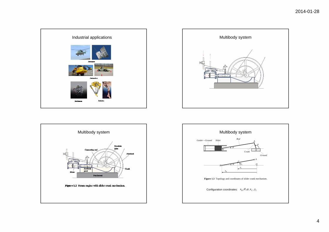
Figure 1.3 Topology and coordinates of slider crank mechanism.
B
AC
Cy
Cx
B
ASlider
Crank
Rod
O
Bx
Guider Ground
Ground
O
, , , ,B C Cx x y Configuration coordinates:
2014-01-28
5
Joints Degrees of freedom and constraints
a) b)
Figure 1.5 a) Three-bar mechanism b) The double pendulum.
B
A D
C
Ground
A
Ground
B
g
Greubler formula
( )m
ii 1
f 3 N 1 r
f 1
Slider crank mechanism:
Three bar mechanism:
Double pendulum:
N 4
( )f 3 4 1 4 2 1
( )f 3 4 1 4 2 1
m 4 ir 2
N m 4 ir 2
N 3 m 2 ir 2
( )f 3 3 1 2 2 2
B
A D
C
Ground
A
Ground
B
g
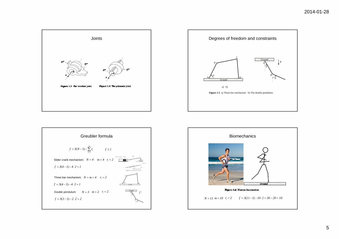
Biomechanics
N 11 m 10 ir 2 ( )f 3 11 1 10 2 30 20 10
2014-01-28
6
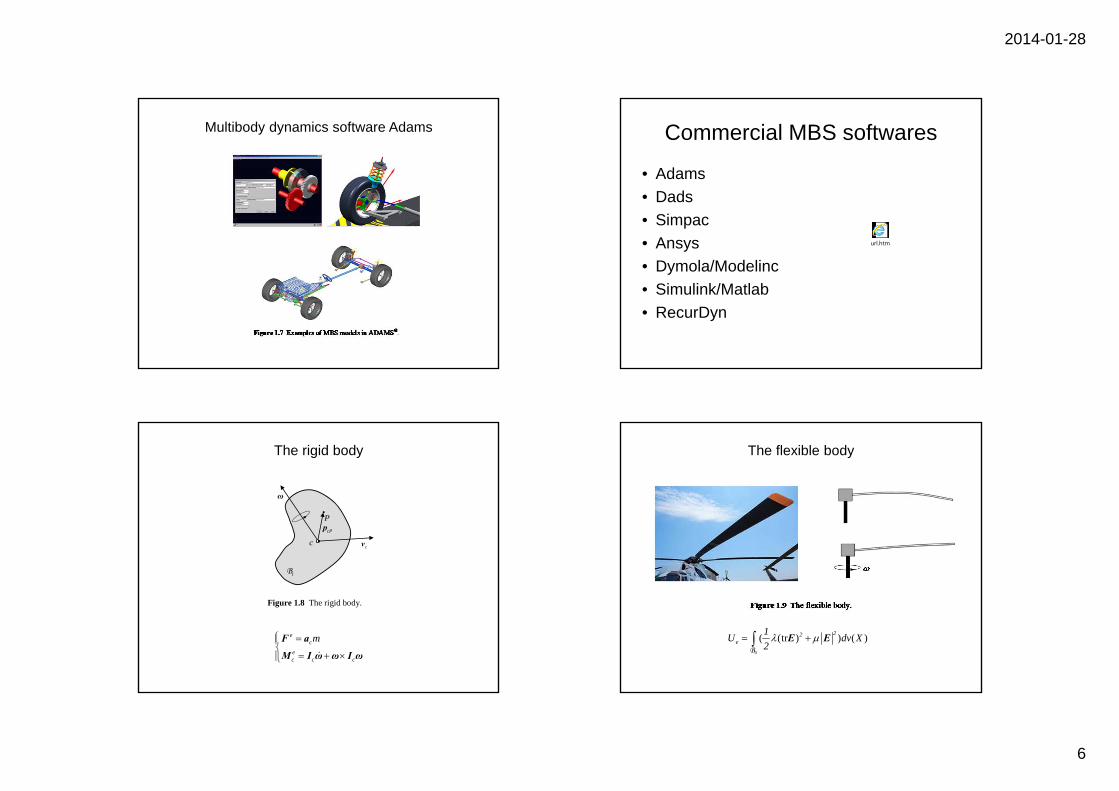
Multibody dynamics software Adams Commercial MBS softwares
• Adams• Dads• Simpac• Ansys• Dymola/Modelinc• Simulink/Matlab• RecurDyn
url.htm
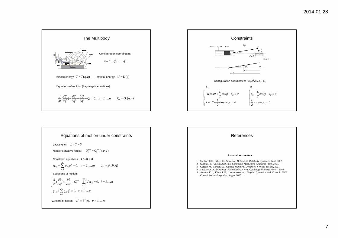
The rigid body
ec
ec c c
m
F a
M I ω ω I ω
Figure 1.8 The rigid body.
ω
P
tB
c cPp
cv
The flexible body
( (tr ) ) ( )0
22e
1U dv X2 E E
B
2014-01-28
7
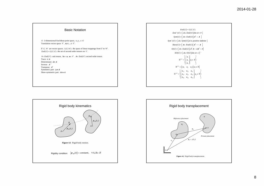
, , ... , 1 2 nq q q q
The Multibody
( , )T T q q ( )U U q
( ) , ,...,kk k k
d T T U Q 0 k 1 ndt q q q
( , )k kQ Q q q
Configuration coordinates:
Kinetic energy: Potential energy:
Equations of motion: (Lagrange’s equations)
Constraints
cos cos
sin sin
C
C
LR x 02
LR y 02
cos
sin
B C
C
Lx x 02
L y 02
A: B:
, , , ,B C Cx x y Configuration coordinates:
Equations of motion under constraints
, ,...,n
k0 k
k 1g g q 0 1 m
( , )k kg g t q
Constraint equations: 1 m n
Equations of motion:
( ) , ,...,
, ,...,
mnonk kk k
1
nk
0 kk 1
d L L Q g 0 k 1 ndt q q
g g q 0 1 m
L T U
( , , )non nonk kQ Q t q q
( ), ,...,t 1 m
Lagrangian:
Nonconservative forces:
Constraint forces:
References
General references
1. Soellner E.E., Führer C.; Numerical Methods in Multibody Dynamics, Lund 2002. 2. Gurtin M.E. An Introduction to Continuum Mechanics. Academic Press. 2003. 3. Geradin M., Cardona A.; Flexible Multibody Dynamics, J. Wiley & Sons, 2001. 4. Shabana A. A.; Dynamics of Multibody Systems. Cambridge University Press, 2005. 5. Åström K.J., Klein R.E., Lennartsson A.; Bicycle Dynamics and Control. IEEE
Control Systems Magazine, August 2005.
2014-01-28
8
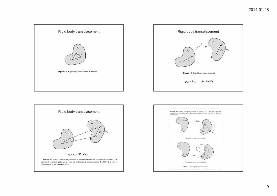
Basic Notation
E :3-dimensional Euclidean point space, , ,..x y E Translation vector space V , , ,...u v V . If U, W are vector spaces. ( )L U,W : the space of linear mappings from to U W .
( ) ( )End L= ,U U U : the set of second order tensors on V .
( )End1 V : unit tensor, , 1u u u V . ( )EndA V second order tensor. Trace: tr A Determinant: det A Inverse: 1A Transpose: TA Symmetric part: symA Skew-symmetric part: skewA
( ) ( )End L= ,U U U ( ) ( ) det End End 0 A A= U U
( ) ( ) TSym End A A A= U U
( ) ( ) Sym Sym is positive definite A A= U U
( ) ( ) TSkew End A A A= U U
( ) ( ) T TO End A A A AA 1= U U
( ) ( ) detSO O 1 A A= U U `
1
3 12 i
3
aa aa
1 31 2 3 ia a a a
11 12 13
3 321 22 23 ij
31 32 33
a a aa a a aa a a
Rigid body kinematics
( ) , ,AB t constant A B p Rigidity condition:
Figure 4.1 Rigid body motion.
0B
B
A
B
( )AB 1tp A
B
( )AB 2tp
Rigid body transplacement Figure 4.2 Rigid body transplacement.
O
A
A
Reference placement
Present placement
0B
B
( )A Ap r Ar
Au
2014-01-28
9
Rigid body transplacement
Figure 4.3 Rigid body in reference placement.
A
0B
a
b
a b
Rigid body transplacement
AB ABp R r
Figure 4.5 Rigid body transplacement.
A
B B
A
0B
B
ABr
AB ABp Rr
( )SOR V
Rigid body transplacement
Theorem 4.1 A rigid body transplacement is uniquely determined by the displacement of (anarbitrary) reduction point A; Au and an orthonormal transformation ( )SOR V which isindependent of the reduction point.
( )P A AP u u R 1 r
Example 4.1 (Plane rigid transplacement, cf. section 4.2.2) The same rigid body transplacement is visualized in both Figure 4.6 a) and 4.6 b) below with different choices of reduction point.
Transplacement with reduction point A.
B
B
A A A
Transplacement with reduction point B.
Figure 4.6 Plane rigid body transplacement.
Au
Bu
A A
B
B B
2014-01-28
10
Summary
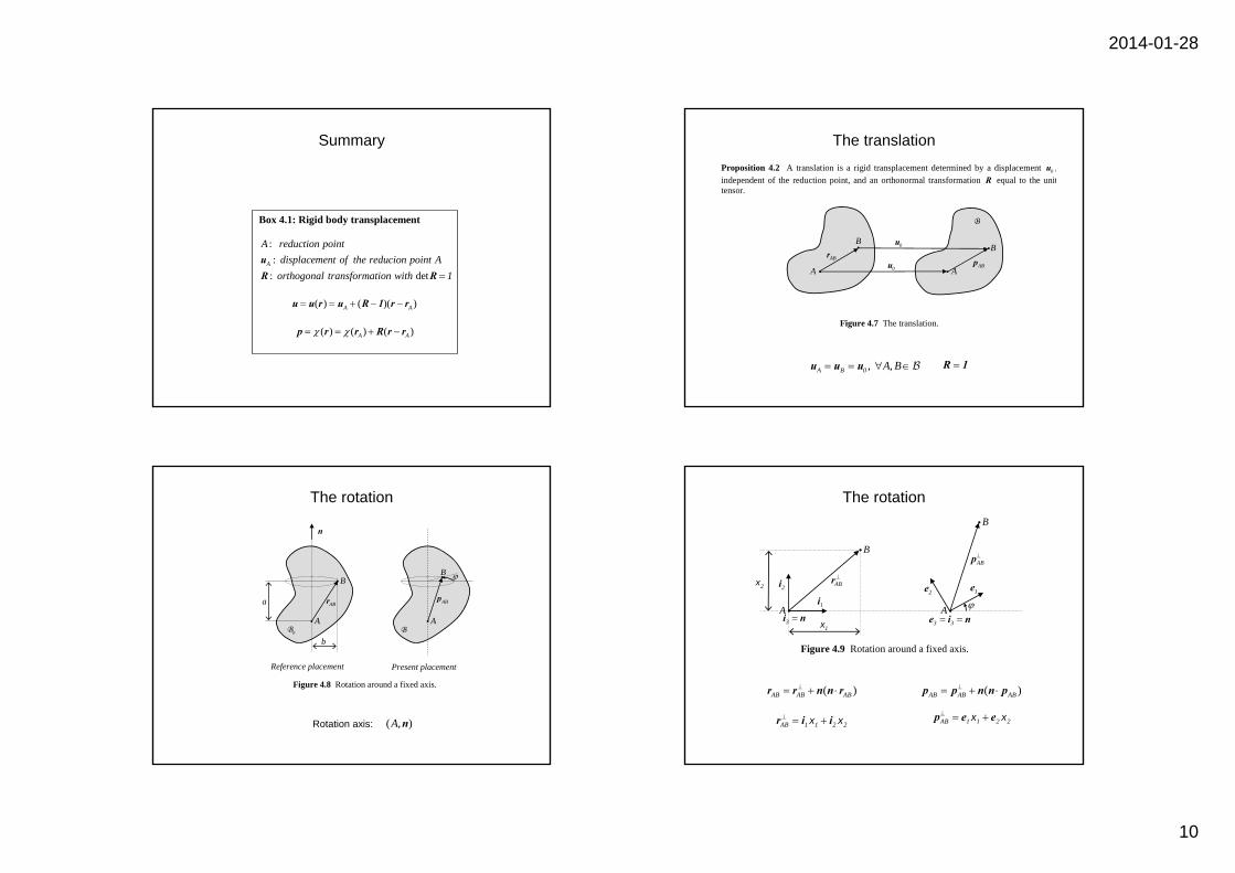
Box 4.1: Rigid body transplacement
: :
: detA
A reduction pointdisplacement of the reducion point A
orthogonal transformation with 1uR R
( ) ( )( )A A u u r u R 1 r r
( ) ( ) ( )A A p r r R r r
The translation
, ,A B 0 A B u u u
Proposition 4.2 A translation is a rigid transplacement determined by a displacement 0u ,independent of the reduction point, and an orthonormal transformation R equal to the unittensor. Figure 4.7 The translation.
0B
A
B
A
B
ABp
0u
0u
B
ABr
R 1
The rotation
( , )A n
Figure 4.8 Rotation around a fixed axis.
Reference placement Present placement
n
B
0B B
B
A A
a
b
ABr ABp
Rotation axis:
The rotation Figure 4.9 Rotation around a fixed axis.
1i 2i AB
r
A
B
3 i n A
1e 2e
B
ABp
3 3 e i n 1x
2x
( )AB AB AB r r n n r
AB 1 1 2 2 r i ix x
( )AB AB AB p p n n p
AB 1 1 2 2 p e ex x
2014-01-28
11
The rotation Figure 4.9 Rotation around a fixed axis.
1i 2i AB
r
A
B
3 i n A
1e 2e
B
ABp
3 3 e i n 1x
2x
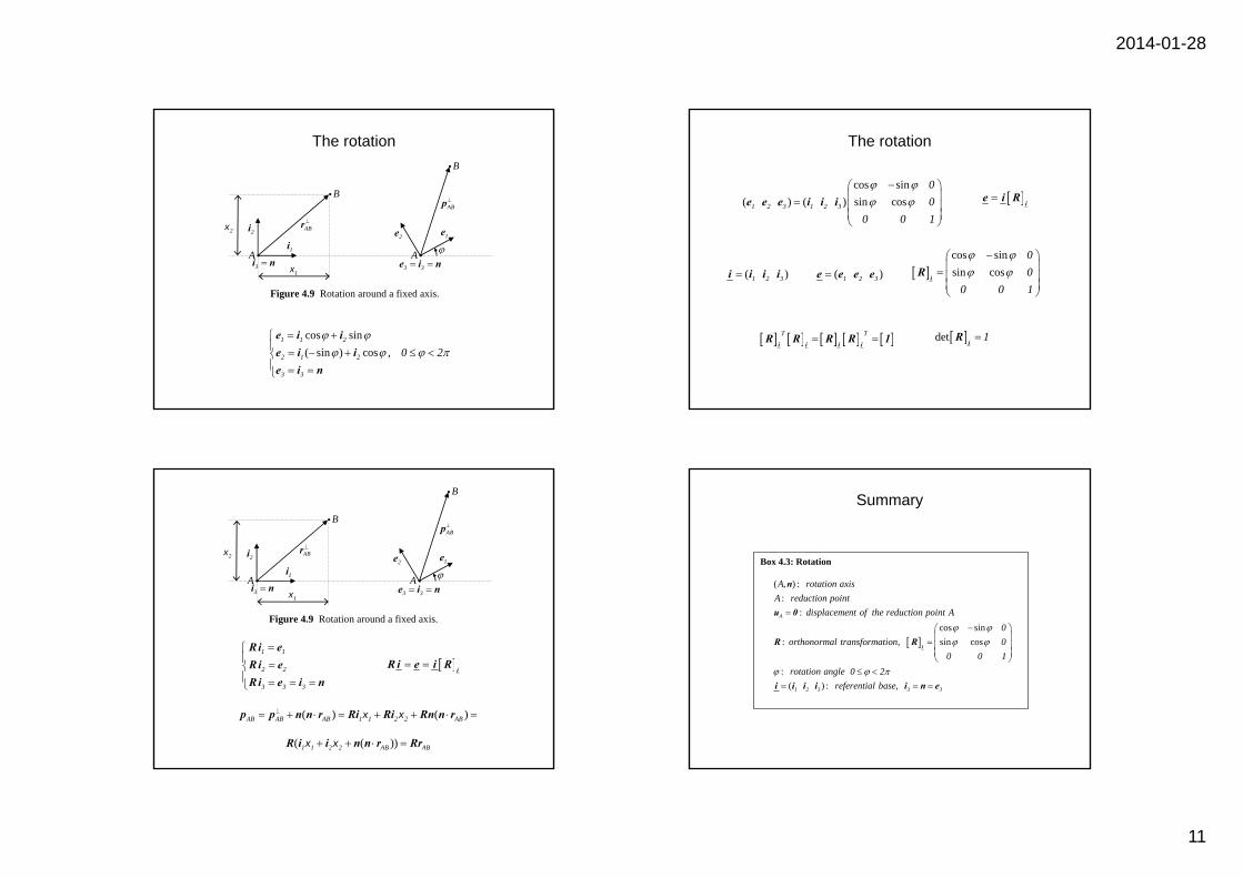
cos sin( sin ) cos ,
1 1 2
2 1 2
3 3
0 2
e i ie i ie i n
The rotation
i
e i R
cos sinsin cos
00
0 0 1
iR( )1 2 3e e e e( )1 2 3i i i i
T T i i i i
R R R R 1 det 1i
R
cos sin( ) ( ) sin cos1 2 3 1 2 3
00
0 0 1
e e e i i i
1 1
2 2
3 3 3
Ri eRi eR i e i n
i
R i e i R
( ) ( )AB AB AB 1 1 2 2 AB p p n n r Ri Ri Rn n rx x
( ( ))1 1 2 2 AB AB R i i n n r Rrx x
Figure 4.9 Rotation around a fixed axis.
1i 2i AB
r
A
B
3 i n A
1e 2e
B
ABp
3 3 e i n 1x
2x
Summary
Box 4.3: Rotation
( , ) : :
: cos sin
: , sin cos
: ( ) :
A
1 2 3
A rotation axisA reduction point
displacement of the reduction point A0
orthonormal transformation 00 0 1
rotation angle 0 2referen
i
n
u 0
R R
i i i i , 3 3tial base i n e

2014-01-28
12
The Euler theorem
A 0B
n
axis ( , )A n
C
i
Theorem 4.2 (The Euler theorem, 1775) Every rigid transplacement with a fixed point isequal to a rotation around an axis through the fixed point.
The canonical representation
cos ( sin ) sin cos1 1 1 2 2 1 2 2 3 3 R i i i i i i i i i i
Rn n
cos sinsin cos
00
0 0 1
iR
( ), 1 2 3 3 i i i i i n
( ) det( ) det( )p R i1 R 1 R
cos sindet sin cos ( )(( cos ) sin )2 2
00 1
0 0 1
,( ) , i1 2 3p 0 1 e R
The characteristic equation, eigenvalues Summary
Box 4.5: Rigid transplacement
: : :
: :
A
A
A reduction pointposition vector of the reduction point in the reference placementdisplacement of the reducion pointposition vector of a material point in the reference placement
p
rurp
: osition vector of a material point in the present placement
rotation tensorR
( ) ( )A A Atranslation rotation
p r r u R r r
2014-01-28
13
Screw representation of the transplacement
Screw line
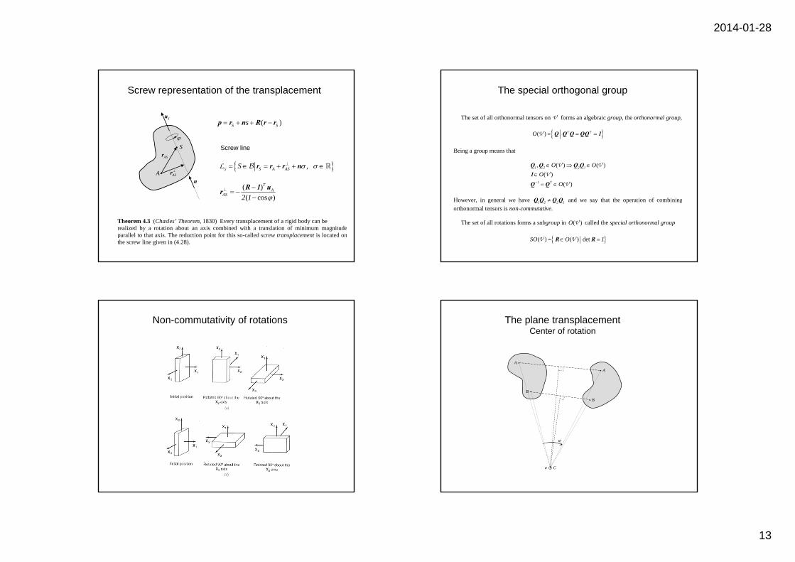
, S A ASS r r r n SL
Su
A
S
n ASr
ASr
Theorem 4.3 (Chasles’ Theorem, 1830) Every transplacement of a rigid body can be realized by a rotation about an axis combined with a translation of minimum magnitudeparallel to that axis. The reduction point for this so-called screw transplacement is located onthe screw line given in (4.28).
( )( cos )
TA
AS 2 1
R 1 ur
( )S Ss p r n R r r
The special orthogonal group
The set of all orthonormal tensors on V forms an algebraic group, the orthonormal group, ( ) T TO Q Q Q QQ 1= V
Being a group means that
, ( ) ( )
( )( )
1 2 2 1
1 T
O OO
O
Q Q Q Q1Q Q
V VV
V
However, in general we have 1 2 2 1Q Q Q Q and we say that the operation of combiningorthonormal tensors is non-commutative. The set of all rotations forms a subgroup in ( )O V called the special orthonormal group ( ) ( ) detSO O 1 R R= V V
Non-commutativity of rotations The plane transplacementCenter of rotation
e
A
A
B
B
C
2014-01-28
14
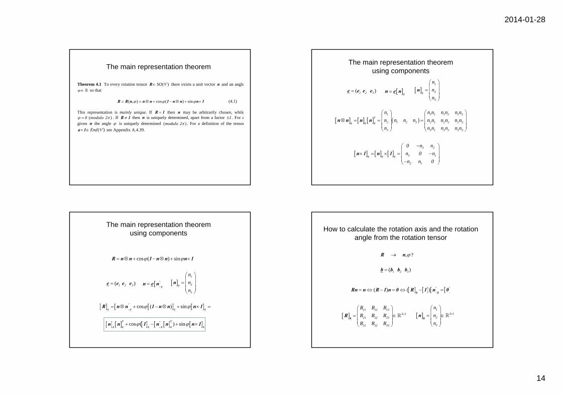
Theorem 4.1 To every rotation tensor ( )SOR V there exists a unit vector n and an angle so that ( , ) cos ( ) sin R R n n n 1 n n n 1 (4.1) This representation is mainly unique. If R 1 then n may be arbitrarily chosen, while
( )0 modulo 2 . If R 1 then n is uniquely determined, apart from a factor 1 . For agiven n the angle is uniquely determined ( )modulo 2 . For a definition of the tensor
( )End a 1 V see Appendix A.4.39.
The main representation theorem
( )1 2 3e e e e 1
2
3
nnn
en
en e n
The main representation theoremusing components
1 1 1 1 2 1 3
T2 1 2 3 2 1 2 2 2 3
3 3 1 3 2 3 3
n n n n n n nn n n n n n n n n nn n n n n n n
e e en n n n
3 2
3 1
2 1
0 n nn 0 nn n 0
e e en 1 n 1
The main representation theoremusing components
cos ( ) sin e e e e
R n n 1 n n n 1
cos ( ) sinT T e e e e e e
n n 1 n n n 1
cos ( ) sin R n n 1 n n n 1
( )1 2 3e e e e 1
2
3
nnn
en
en e n
How to calculate the rotation axis and the rotation angle from the rotation tensor
( ) ( ) b b
Rn n R 1 n 0 R 1 n 0
11 12 13
3 321 22 23
31 32 33
R R RR R RR R R
bR
, ?R n
1
3 12
3
nnn
bn
( )1 2 3b b b b

2014-01-28
15
The eigenvalue problem
11 12 13 1 1
21 22 23 2 2
31 32 33 3 3
R 1 R R n 0 nR R 1 R n 0 nR R R 1 n 0 n
n
cos11 22 33tr R R R 1 2 R
arccos( ) arccos( )
arccos( )
11 22 33
11 22 33
R R R 1tr 12 2
R R R 122
R
Coordinate representations of ( )SO V
• Euler angles• Bryant angles• Euler parameters• Quaternions• ……
Euler angles: First rotation
01e
02e
03 3f e
1f
2f
cos sin
( ) sin coso3
00
0 0 1
eR ( ) ( ) o
o o3 3
ef R e e R
( )0 0 0 01 2 3e e e e
( )1 2 3f f f f
Euler angles: Second rotation
3g 3f
1 1g f
2f
2g
( ) cos sinsin cos
1
1 0 000
fR ( ) ( )1 1
fg R f f R
( )1 2 3f f f f
( )1 2 3g g g g
2014-01-28
16
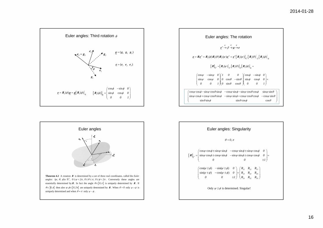
Euler angles: Third rotation
2e
1e
3 3e g
1g
2g
( ) ( )3 3 g
e R g g R cos sin
( ) sin cos3
00
0 0 1
gR
( )1 2 3g g g g
( )1 2 3e e e e
Euler angles: The rotation
( ) ( ) ( ) ( ) ( ) ( )oo o o
3 1 3 3 1 3 e f g
e Re R R R e e R R R
( ) ( ) ( )o o3 1 3 e e f g
R R R R
cos sin cos sinsin cos cos sin sin cos
sin cos
0 1 0 0 00 0 0
0 0 1 0 0 0 1
cos cos sin cos sin cos sin sin cos cos sin sinsin cos cos cos sin sin sin cos cos cos cos sin
sin sin sin cos cos
o e f g e
Euler angles
Theorem 4.2 A rotation R is determined by a set of three real coordinates, called the Eulerangles: ( , , ) , , , 3 0 2 0 0 2 . Conversely these angles areessentially determined by R . In fact the angle ,0 is uniquely determined by R . If
,0 then also , ,0 2 are uniquely determined by R . When 0 only isuniquely determined and when only .
cos cos sin sin cos sin sin cossin cos cos sin sin sin cos coso
00
0 0 1
eR
cos( ) sin( )sin( ) cos( )
11 12 13
21 22 23
31 32 33
0 R R R0 R R R
0 0 1 R R R
Euler angles: Singularity
Only is determined. Singular!
,0
2014-01-28
17
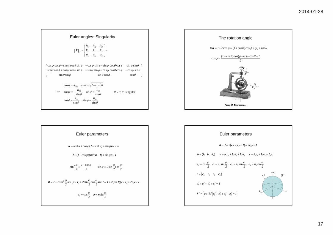
Euler angles: Singularity
cos , sin cos
cos , sinsin sin
cos , sinsin sin
233
23 13
32 31
R 1R R
R R
o
11 12 13
21 22 23
31 32 33
R R RR R RR R R
eR
cos cos sin cos sin cos sin sin cos cos sin sinsin cos cos cos sin sin sin cos cos cos cos sin
sin sin sin cos cos
, singular0
The rotation angle
( cos )cos( ) coscos 1 12
cos ( cos )cos( ) costr 1 2 1 R
Euler parameters
sin ( ) sin cos ( )( )202 2 2 2e
2 2 2
R 1 n n 1 n 1 1 e 1 e 1 e 1
cos , sin0e2 2
e n
cos ( ) sin R n n 1 n n n 1
( cos )( ) sin1 1 n n 1 n 1
cossin2 12 2 sin sin cos2
2 2
Euler parameters
( )1 2 3b b b b 1 1 2 2 3 3n n n n b b b 1 1 2 2 3 3e e e e b b b
cos , sin , sin , sin0 1 1 2 2 3 3e e n e n e n2 2 2 2
3 4 2 2 2 20 1 2 3S e e e e e 1
2 2 2 20 1 2 3e e e e 1
3S
0e
3e4 0 1 2 3e e e e e
( )( ) 02 2e R 1 e 1 e 1 e 1
2014-01-28
18
3 2
0 3 1
2 1
0 e e2e e 0 e
e e 0
( )3 2 3 2
3 1 3 1
2 1 2 1
1 0 0 0 e e 0 e ee 0 1 0 2 e 0 e e 0 e
0 0 1 e e 0 e e 0
bR
( ) ( , ), ( , ) 30 0e e e e S R R R e e
( ) ( ) ( )( ) ( ) ( )( ) ( ) ( )
2 20 1 1 2 0 3 1 3 0 2
2 21 2 0 3 0 2 2 3 0 1
2 21 3 0 2 2 3 0 1 0 3
2 e e 1 2 e e e e 2 e e e e2 e e e e 2 e e 1 2 e e e e2 e e e e 2 e e e e 2 e e 1
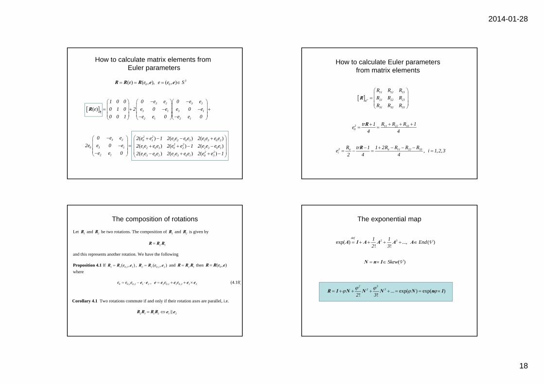
How to calculate matrix elements fromEuler parameters
o
11 12 13
21 22 23
31 32 33
R R RR R RR R R
eR
, , ,2 ii ii 11 22 33i
R 1 2R R R Rtr 1e i 1 2 32 4 4
R
How to calculate Euler parameters from matrix elements
2 11 22 330
R R R 1tr 1e4 4
R
The composition of rotations
Let 1R and 2R be two rotations. The composition of 1R and 2R is given by 2 1R R R and this represents another rotation. We have the following Proposition 4.1 If ,( , )1 1 0 1 1eR R e , ,( , )2 2 0 2 2eR R e and 2 1R R R then ( , )0eR R e where , ,0 0 1 0 2 1 2e e e e e , , ,2 0 1 1 0 2 1 2e e e e e e e (4.18)
Corollary 4.1 Two rotations commute if and only if their rotation axes are parallel, i.e. 2 1 1 2 1 2 R R R R e e
The exponential map
exp( ) ..., ( )! !
def2 31 1 End
2 3 A 1 A A A A V
... exp( ) exp( )! !
2 32 3
2 3 R 1 N N N N n 1
( )Skew N n 1 V
2014-01-28
19
O
A
A
Reference placement
Present placement 0B
tB
( )A A tp pAr
P
P
Pr
( )P P tp p
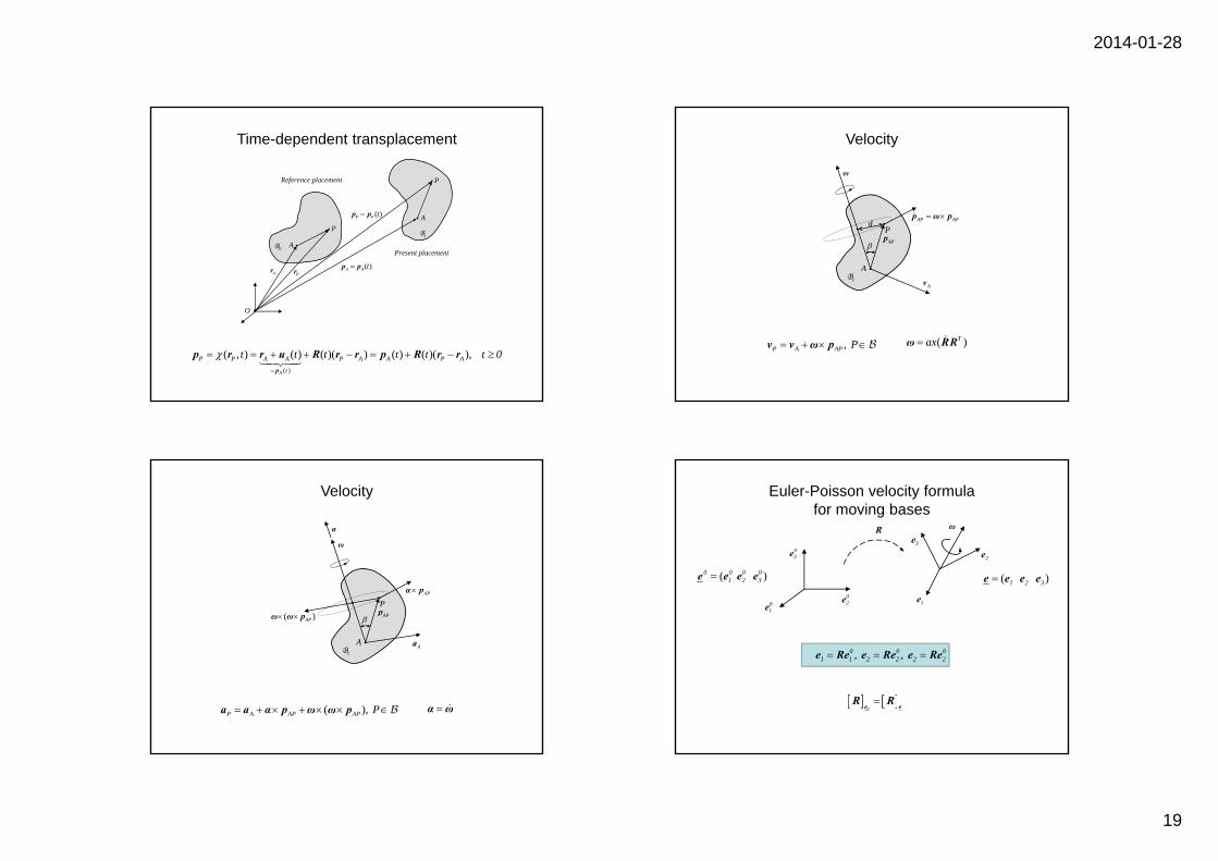
Time-dependent transplacement
( )
( , ) ( ) ( )( ) ( ) ( )( ), A
P P A A P A A P A
t
t t t t t t 0
p
p r r u R r r p R r r
Velocity
, P A AP P v v ω p ( )Taxω RR
ω
P
tBA
APp
Av
d AP AP p ω p
α ω( ), P A AP AP P a a α p ω ω p
α
ω
P
tBA
APp
Aa
APα p
( )AP ω ω p
Velocity
01e
02e
03e
1e
2e3e
ωR
Euler-Poisson velocity formulafor moving bases
, , 0 0 01 1 2 2 2 2 e Re e Re e Re
( )1 2 3e e e e( )0 0 0 01 2 3e e e e
0
e eR R

2014-01-28
20
01e
02e
03e
1e
2e3e
ωR
Euler-Poisson velocity formulafor moving bases
Theorem 4.4 (Euler-Poisson velocity formula for moving bases) , , ,i i i 1 2 3 e ω e (4.32) where
3
i ii 1
12
ω e e (4.33)
Euler-Poisson velocity formulafor moving vectors and tensors
,
( ) ( ) ( ) ( )3
j iji j 1
t t t A t
iA A e e
( ) rel A ω A A ω 1 A
rel a ω a a
3
reli
i 1a
iea e a
( ) ( ) ( )3
ii 1
t t a t
ia a e
,
( ) ( ) ( )3
relj ij
i j 1
t t A t
ieA e e A
Proposition 4.6 The angular velocity ω , expressed in Euler angles, is given by 1 1 2 2 3 3 ω e e e where
sin sin cos
sin cos sin
cos
1
2
3
(4.39)
and ( )1 2 3e e e e is an RON-basis following the rotation of the rigid body (‘fixed to thebody’).
Angular velocity and Euler angles Combining rotationsThe addition of angular velocities, version 1
( )T1 1 1axω R R
( )1 1 tR R
2 2 1 ω ω R ω
( )2 2 tR R 2 1R R R
( )T2 2 2axω R R ( )Taxω RR
2014-01-28
21
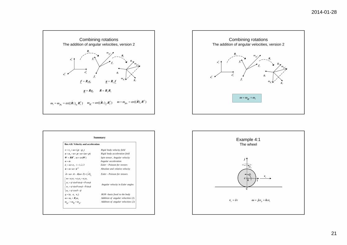
Combining rotationsThe addition of angular velocities, version 2
1R
2R
1f
2f 3f
1g
2g
3g
0feω
0geω
gfω
01e
02e
03e
(( ) )T2 2axgf fω R R
1 0f R e 2g R f
(( ) )0 0
T11 1ax fe eω ω R R
(( ) )0
Teax geω ω R R
0g Re 2 1R R R
Combining rotationsThe addition of angular velocities, version 2
1R
2R
1f
2f 3f
1g
2g
3g
0feω
0geω
gfω
01e
02e
03e
1 gfω ω ω
Summary
Box 4.8: Velocity and acceleration
( ) ( )
, ( ) ,
A A
AT
Rigid body velocity fieldRigid body acceleration field
ax Spin tensor Angular velocity
v v ω p pa a α p ω ω p
W RR ω Wα ω
, , ,
i i
rel
Angular accelerationi 1 2 3 Euler Poisson for vectors
Absolute and
e ω e
u ω u u
( )
sin sin cos
sin cos sin
cos
1 1 2 2 3 3
1
2
3
relative velocity
Euler Poisson for tensors
Angular velocity in Euler angles
eA ω A A ω 1 A
ω e e e
e ( ) - ( )
0 0
1 2 3
2 2 1
RON basis fixed to the bodyAddition of angular velocities 1
gfge fe
e e eω ω R ωω ω ω ( ) Addition of angular velocities 2
Example 4:1The wheel
c vv i p r ω j k
2014-01-28
22
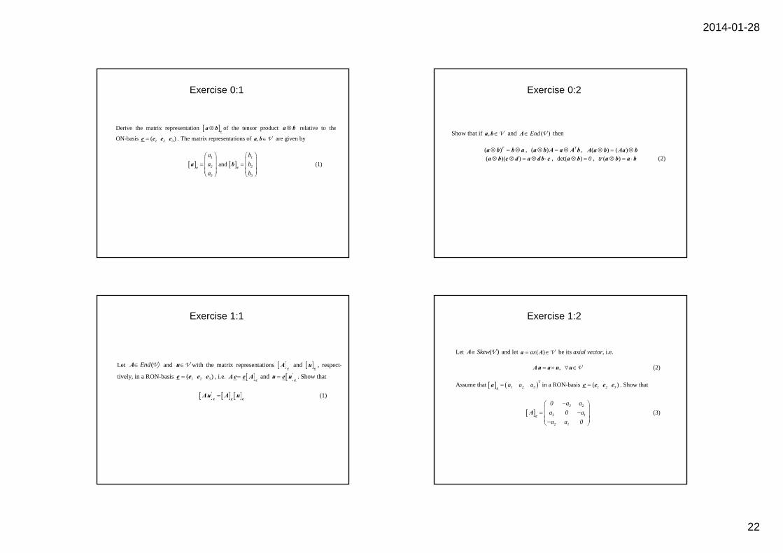
Derive the matrix representation e
a b of the tensor product a b relative to the
ON-basis ( )1 2 3e e e e . The matrix representations of , a b V are given by
1
2
3
aaa
ea and
1
2
3
bbb
eb (1)
Exercise 0:1
Show that if , a b V and ( )EndA V then ( )T a b b a , ( ) T a b A a A b , ( ) ( ) A a b Aa b ( )( ) a b c d a d b c , det( ) 0 a b , ( )tr a b a b (2)
Exercise 0:2
Let (EndA V) and u V with the matrix representations eA and e
u , respect-
tively, in a RON-basis ( )1 2 3e e e e , i.e. e
A e e A and e
u e u . Show that
e e e
Au A u (1)
Exercise 1:1
Let ( )SkewA V and let ( )ax a A V be its axial vector, i.e.
, A u a u u V (2)
Assume that T1 2 3a a ae
a in a RON-basis ( )1 2 3e e e e . Show that
3 2
3 1
2 1
0 a aa 0 aa a 0
eA (3)
Exercise 1:2
2014-01-28
23
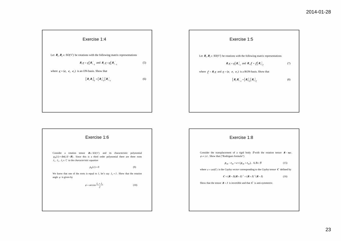
Exercise 1:4
Let , ( )1 2 SOR R V be rotations with the following matrix representations 1 1
eR e e R and 2 2
eR e e R (5)
where ( )1 2 3e e e e is an ON-basis. Show that 2 1 2 1
e e eR R R R (6)
Exercise 1:5
Let , ( )1 2 SOR R V be rotations with the following matrix representations
1 1e
R e e R and 2 2f
R f f R (7)
where 1f R e and ( )1 2 3e e e e is a RON-basis. Show that
2 1 1 2e e f
R R R R (8)
Consider a rotation tensor ( )SOR V and its characteristic polynomial ( ) det( )p R 1 R . Since this is a third order polynomial there are three roots , , 1 2 3 to the characteristic equation ( )p 0 R (9) We know that one of the roots is equal to 1, let’s say 3 1 . Show that the rotation angle is given by
arccos 1 2
2
(10)
Exercise 1:6 Exercise 1:8
Consider the transplacement of a rigid body with the rotation tensor R n , . Show that (“Rodrigues formula”) ( ), ,AB AB AB AB A B p r c p r (15) where ( )axc C is the Cayley vector corresponding to the Cayley tensor C defined by ( )( ) ( ) ( )1 1 C R 1 R 1 R 1 R 1 (16) Show that the tensor R 1 is invertible and that C is anti-symmetric.
2014-01-28
24
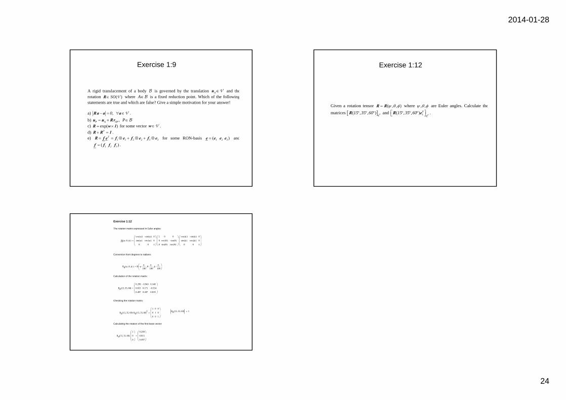
A rigid translacement of a body is governed by the translation A u V and the rotation ( )SOR V where A is a fixed reduction point. Which of the following statements are true and which are false? Give a simple motivation for your answer!
a) , 0 Ra a a V . b) , P A AP P u u Rr c) exp( ) R w 1 for some vector w V . d) T R R 1 . e) T
1 1 2 2 3 3 R f e f e f e f e for some RON-basis ( )1 2 3e e e e and ( )1 2 3f f f f .
Exercise 1:9
Given a rotation tensor ( , , ) R R where , , are Euler angles. Calculate thematrices ( , , ) 015 35 60
eR and ( , , ) 0
0115 35 60 e
R e .
Exercise 1:12
Exercise 1:12
The rotation matrix expressed in Euler angles:
R ( )
cos ( )
sin ( )
0
sin ( )
cos ( )
0
0
0
1
1
0
0
0
cos ( )
sin ( )
0
sin ( )
cos ( )
cos ( )
sin ( )
0
sin ( )
cos ( )
0
0
0
1
Conversion from degrees to radians:
Rd ( ) R
180
180
180
Calculation of the rotation matrix:
Rd 15 35 60( )
0.299
0.815
0.497
0.943
0.171
0.287
0.148
0.554
0.819
Checking the rotation matrix:
Rd 15 35 60( ) 1Rd 15 35 60( ) Rd 15 35 60( )T
1
0
0
0
1
0
0
0
1
Calculating the rotation of the first basis vector:
Rd 15 35 60( )
1
0
0
0.299
0.815
0.497