20111223 Multi-objective optimisation methodology …...solution space. A Pareto optimal solution...

Lijie Cui, Jakin Ravalico, George Kuczera, Graeme Dandy and Holger Maier

Technical Report

23 December 2011

Multi-objective Optimisation Methodology for the Canberra

Water Supply System

ii Multi-objective Optimisation Methodology for the Canberra Water Supply System

Copyright Notice

© eWater Ltd 2011

Legal Information

This work is copyright. You are permitted to copy and reproduce the information, in an

unaltered form, for non-commercial use, provided you acknowledge the source as per the

citation guide below. You must not use the information for any other purpose or in any

other manner unless you have obtained the prior written consent of eWater Ltd.

While every precaution has been taken in the preparation of this document, the publisher

and the authors assume no responsibility for errors or omissions, or for damages

resulting from the use of information contained in this document. In no event shall the

publisher and the author be liable for any loss of profit or any other commercial damage

caused or alleged to have been caused directly or indirectly by this document.

Citing this document

Cui, L., Ravalico, J., Kuczera, G., Dandy, G. and Maier, H. (2011). Multi-objective

Optimisation Methodology for the Canberra Water Supply System. eWater Cooperative

Research Centre, Canberra.

Publication date: December 2011 (Version 1.0)

ISBN: 978-1-921543-52-4

Acknowledgments

eWater CRC acknowledges and thanks all partners to the CRC and individuals who have

contributed to the research and development of this publication.

The contributions of the following individuals to the drafting of this document are

gratefully acknowledged: Mathew J. Hardy.

For more information:

Innovation Centre, Building 22

University Drive South

Bruce, ACT, 2617, Australia

T: 1300 5 WATER (1300 592 937)

T: +61 2 6201 5834 (outside Australia)

E: [email protected]

www.ewater.com.au

Multi-objective Optimisation Methodology for the Canberra Water Supply System iii

Contents 1 Introduction ................................................................. 1

2 Multiobjective optimisation .......................................... 2

2.1 Pareto dominance approach ................................................................................................. 3

2.2 Evolutionary multiobjective optimisation algorithms.............................................................. 5

e-MOGA Algorithms .............................................................................................................. 5

Non-dominated Sorting Genetic Algorithm II (NSGA-II)........................................................ 8

3 WATHNET Simulation model .................................... 10

3.1 WATHNET Overview .......................................................................................................... 10

3.2 Network Linear Programs ................................................................................................... 10

3.3 Example of Network Operation ........................................................................................... 13

3.4 Description of the WATHNET Program .............................................................................. 13

4 Case Study – Canberra regional water network ....... 15

4.1 Canberra Water Supply System ......................................................................................... 15

4.2 Optimisation Objectives and Decision Variables ................................................................ 18

4.3 Performance Measures – Three Metrics............................................................................. 20

4.4 Results and Discussion....................................................................................................... 21

Case 1................................................................................................................................. 22

Results for Case 2 .............................................................................................................. 25

Performance comparison .................................................................................................... 30

5 Conclusion ................................................................ 34

6 References ................................................................ 35

Multi-objective Optimisation Methodology for the Canberra Water Supply System 1

1 Introduction Making decisions for management of urban water supply headworks systems is a complex

and difficult task. Typically, such systems have not only multiple users (urban, irrigation, and

environmental) with different (often conflicting) objectives and risk tolerances, but also

multiple sources with different levels of quality. This complexity gives rise to a very large

number of infrastructure and operating policy options. The solution to these complex

decision problems requires the use of mathematical techniques that are formulated to take

simultaneous consideration of conflicting objectives. Furthermore, there is a very large

element of uncertainty and risk in all water supply decisions due to hydrological, climatic and

anthropogenic uncertainty and an inability to predict the future with reasonable accuracy.

Traditionally, these types of problems are formulated as single-criterion problems whose

goal is to find the ‘best’ solution that corresponds to the minimum or maximum value by

imposing constraints on the other criteria, or by incorporating multiple criteria into a single

objective function using weighting factors. In this case a compromise between the criteria

has to be defined a priori. For a multiobjective problem, there is usually no single solution for

which all objectives are optimal. There exists a set of alternative solutions (Pareto optimal

solution set) for which holds that there are no other solutions that are superior when all

objectives are considered simultaneously. The most common method is to choose the best

trade-offs among all the defined objectives that are in conflict with each other. Hence, the

purpose of optimizing a multiobjective problem is to find Pareto optimal solutions.

Multi-objective optimisation (MO) problems have received increasing interest from

researchers with various backgrounds since the early 1960s. Over recent years there has

been an increase in the application of genetic algorithms to solving multi-objective

optimisation problems. Genetic algorithms (GAs) are designed to mimic Darwinian survival of

the fittest using operators such as mutation and crossover on a population of potential

solutions to reproduce natural evolutionary behaviour and drive the solutions towards the

system optimum. Since GAs use a population of solutions, they are particularly suited to

multi-objective optimisation where several solutions are desired. GAs are also well suited to

searching intractably large, poorly understood problem spaces, due to the inclusion of the

mutation operator, which increases the diversity of the search. The first implementation of a

multiobjective optimisation algorithm (MOEA) was that of Schaffer (1984), while Goldberg

(1989) suggested a new non-dominated sorting procedure using the concept of domination

to give preference to non-dominated individuals in the population. Since then, research

interests in this field have remained strong and a variety of multiobjective optimisation

techniques have been developed.

This study aims to (1) demonstrate the applicability of multiobjective optimisation methods to

an urban water supply system; (2) compare the performance of the two recent genetic

optimisation methods, NSGAII and εMOGA. The report first describes the principles of multi-

objective optimisation. This is followed by a case study involving the Canberra water supply

system demonstrating the application of the multiobjective objection procedure. Finally, the

results are presented and discussed and conclusions are drawn.

2 Multi-objective Optimisation Methodology for the Canberra Water Supply System

2 Multiobjective optimisation Most realistic optimisation problems, particularly those in design, require the simultaneous

optimisation of more than one objective function. Conflicting objectives introduce trade-off

solutions and make the task complex yet interesting to execute. Multiobjective optimisation

methods deal with the process of simultaneously optimizing two or more conflicting

objectives subject to certain constraints.

The classical way of tackling multiobjective problems converts multiple objectives into a

single objective and solves for the optimal solution. There are several drawbacks to this

method. Conversion of multiple objectives into a single objective necessitates scaling of

objectives to ensure that all objectives are comparable. Also any weighting of priorities

needs to occur before the optimisation is performed, leaving the final result dependent on

weightings, which are generally subjective. Further, since classical single objective

optimisation methods are used to solve the converted problem, only one solution is found.

Hence a thorough exploration of the trade off between different objectives requires many

optimisation runs to be carried out.

To combat these shortcomings, multi-objective optimisation using a Pareto dominance

approach can be implemented. This approach is explained in detail in the next section. The

Pareto dominance approach compares the value of objectives in a solution only with values

of the same objective in different solutions, thus there is no need for scaling or weighting of

objectives. A solution is considered to be Pareto dominant if it is better than another solution

in one objective, and at least equal in all other objectives. Consequently there will be several

dominant solutions in a single optimisation problem, which provides a decision maker with

the ability to select from a wide range of solutions that represent preferences towards

different objectives.

The multi-objective optimisation problem is often formulated as follows:

( )

,...,K,kxxx

,...,J,j(x)h

,...,I,i(x)g

Mnxobj

U

kk

L

k

j

i

n

21

210

210

:toSubject

,,2,1

:objectives M Minimise

=≤≤

==

=≥

= K

(1)

Equation 1 is a minimization problem (all objectives that are to be maximised are multiplied

by -1). A solution x is defined as a vector of K decision variables with lower and upper

bounds xL and x

U respectively. The problem is subject to I inequality and J equality

constraints.


2.1 Pareto dominance approach

A key characteristic of MO analysis is that optimisation cannot only consider a single

objective because performance in other objectives may suffer. Optimality in the context of

multiobjective global optimisation using a dominance approach was originally defined by and

named after Vilfredo Pareto (Pareto 1896). In a multiobjective optimisation problem, the

presence of conflicting objectives gives rise to a set of optimal solutions (called Pareto-

optimal solutions), instead of a single optimal solution. In the absence of any priority towards

any particular objective, all Pareto-optimal solutions become equally important to the user.

Thus, it is essential that a multiobjective optimisation algorithm find a wide variety of Pareto-

optimal solutions, instead of just one of them find a diverse subset of the Pareto-optimal

solutions.

If all objective functions are minimized, a feasible solution x is said to dominate another

feasible solution y, if and only if:

)()( yObjxObj ii ≤ for i = (1,…,M) and;

)()( yObjxObjjj

< for least one objective function J.

A solution is said to be Pareto optimal if it is not dominated by any other solution in the

solution space. A Pareto optimal solution cannot be improved with respect to any objective

without worsening at least one other objective. The set of all feasible non-dominated

solutions in X is referred to as the Pareto optimal set; and for a given Pareto optimal set, the

corresponding objective function values in the objective space are called the Pareto front.

For many problems, the number of Pareto optimal solutions is extremely large. This is

illustrated in Figure 1, which shows solutions from a two objective optimisation, plotted in

objective space. The solutions from the third sampling, are considered to be Pareto

dominant, since there are no other known solutions which outperform them in both

objectives, and any increase in one of the objectives will result in a decrease in the other

objective. These solutions are known as the Pareto front. In the situation where it is known

that there are no other solutions in existence which dominate those in the Pareto front, the

Pareto front can also be termed the True front (PFTRUE), the Pareto Optimal set, the

admissible set and the efficient points. It should be noted here that the set of solutions found

by a GA is unlikely to be the True front, since it does not provide an exhaustive search of the

solution space; however use of the appropriate GA parameters should allow a close

approximation of the True front. Thus the set of solutions that is returned from a multi-

objective GA, should be referred to as the approximate Pareto set, or front. It is important to

recognise that while all solutions A-E shown in Figure 1 are optimal solutions, it is still

possible for a decision maker to have a preference towards a particular Pareto solution,

based on their own priorities regarding the importance of the two competing objectives. The

strength of the Pareto dominance approach to multi-objective optimisation is that a variety of

solutions which preference different objectives are returned, with the decision maker having

access to all solutions, such that the weighting of priorities can occur a posteriori.


The ultimate goal of a multi-objective optimisation algorithm is to identify solutions in the

Pareto optimal set. However, for many multi-objective problems, identifying the entire Pareto

optimal set is practically impossible due to its size. In addition, for many problems, especially

for combinatorial optimisation problems, proof of solution optimality is computationally

infeasible. Therefore, a practical approach to multi-objective optimisation is to investigate a

set of solutions (the best-known Pareto set) that represent the Pareto optimal set as well as

possible. With these concerns in mind, a multi-objective optimisation approach should

achieve the following three conflicting goals (Zitler, 2000):

1 The best-known Pareto front should be as close as possible to the true Pareto front.

Ideally, the best-known Pareto set should be a subset of the Pareto optimal set.

2 Solutions in the best-known Pareto set should be uniformly distributed and diverse

over the Pareto front in order to provide the decision-maker with a true picture of

trade-offs.

3 The best-known Pareto front should capture the whole spectrum of the Pareto front.

This requires investigating solutions at the extreme ends of the objective function

space.

For a given computational time limit, the first goal is best served by focusing the search on a

particular region of the Pareto front. On the contrary, the second goal demands the search

effort to be uniformly distributed over the Pareto front. The third goal aims at extending the

Pareto front at both ends, exploring new extreme solutions.

C

Ist sampling

2nd sampling

3rd sampling

Maximizing objective 1

Maxim

izin

g o

bje

ctive 2

Example of non-dominated points, also called

Pareto frontier (PFTRUE)

D

E

Figure 1. Example showing the concept of the Pareto front


2.2 Evolutionary multiobjective optimisation algorithms

A number of stochastic optimisation techniques like simulated annealing, tabu search, and

ant colony optimisation could be used to generate the Pareto set. However, evolutionary

algorithms (EAs) are a natural choice for solving multiobjective optimisation problems.

Evolutionary algorithms are characterized by a population of solution candidates and the

reproduction process enables the combination of existing solutions to generate new

solutions. Finally, natural selection determines which individuals of the current population

participate in the new population. One of the advantages of evolutionary algorithms is that

they require very little knowledge about the problem being solved, are easy to implement

and robust and can be implemented in a parallel environment.

Figure 2 shows a flowchart of the evolutionary algorithm process. After the pioneering work

on multiobjective evolutionary optimisation in the eighties (Goldberg and Kuo 1989), several

different algorithms have been proposed and successfully applied to various problems.

Figure 2. Flowchart of evolutionary algorithm process

Although the possibility of using EAs to solve multiobjective optimisation problems was

proposed in the seventies, David Schaffer first implemented vector evaluated genetic

algorithms (VEGAs) in 1984. There was lukewarm interest in the field for a decade, but this

began to change in 1993 following a suggestion by David Goldberg based on the use of the

non-domination concept and a diversity-preserving mechanism. There exists a number of

variants of these algorithms and they have been applied to many real world problems from

science and engineering. This case study considers two of the most recent evolutionary

algorithms. The following sections describe the key features of these two algorithms.

e-MOGA Algorithms

According to Deb et al. (2003), multiobjective optimisation has two fundamental goals:

guiding the search towards finding a non-dominated set of solutions as close as possible to

the Pareto optimal front, and keeping a diverse set of non-dominated solutions. εMOGA was

one of the recent advances using the concept of the ε-dominance to achieve the above goals

(Laumanns et al. 2002).


Definition 1 (Dominance relation)

Let f, g ∈ IRm

. Then f is said to dominate g, denoted as gf f

, if

{ } ii gfmi ≥∈∀ :,...1

2. { }

jj gfmj ≥∈∃ ,...1

Based on the concept of dominance, the Pareto set can be defined as follows.

Definition 2 (Pareto set)

Let F ⊆ IRm

be a set of vectors. Then the Pareto set F ∗ ⊆F is defined as follows: F ∗

contains all vectors Fg ∈

which are not dominated by any vector f ∈ F , i.e.

F ∗ := {g ∈ F | ∃f ∈ F : f > g}} (2)

Vectors in F ∗ are called Pareto vectors of F . The set of all Pareto sets of F is denoted as

P ∗(F ).

From the above definition we can easily deduce that any vector g ∈ F \ F ∗ is dominated by at

least one f ∈ F ∗, i.e.

**:\ FfFFg ∈∃∈∀ such that

gf f. (3)

For a given set F, the set F ∗ is unique. Therefore, we have P∗(F ) = {F∗}.

For many sets F, the Pareto set F* is of substantial size. Thus, the numerical determination

of F* is prohibitive, and F* as a result of an optimisation is questionable. Moreover, it is not

clear at all what a decision maker can do with such a large result of an optimisation run.

What would be more desirable is an approximation of F* which approximately dominates all

elements of F and is of (polynomially) bounded size. This set can then be used by a decision

maker to determine interesting regions of the decision and objective space which can be

explored in further optimisation runs. Next, we define a generalization of the dominance

relation.

Definition 3 (ε -Dominance)

Let f, g ∈ IR+ m

f is said to ε -dominance g for some ε > 0, gf εf

For all },...,1{ mi ∈

ii gf f)1( ε+ (4)

The set of all of ε-approximate Pareto sets of F is denoted as )(FPε .

The concept of ε-dominance has been found to be an efficient mechanism for maintaining

diversity in multiobjective optimisation problems without losing convergence properties


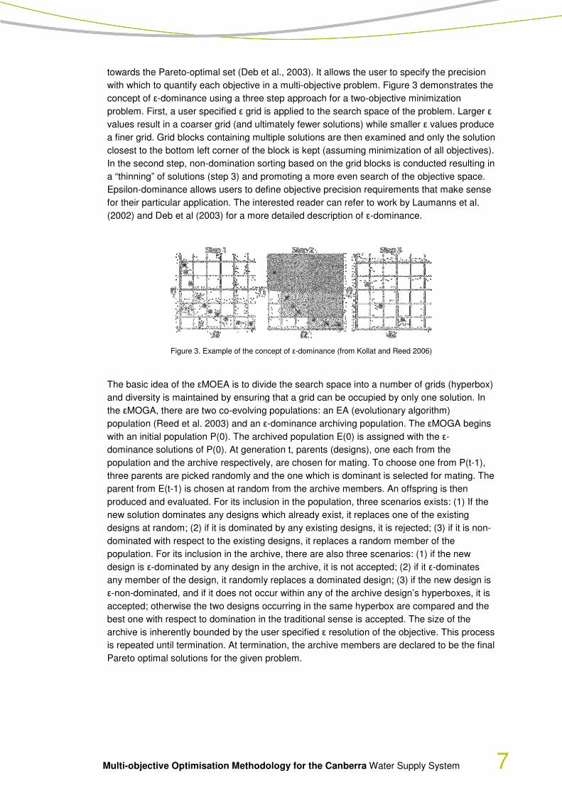
towards the Pareto-optimal set (Deb et al., 2003). It allows the user to specify the precision

with which to quantify each objective in a multi-objective problem. Figure 3 demonstrates the

concept of ε-dominance using a three step approach for a two-objective minimization

problem. First, a user specified ε grid is applied to the search space of the problem. Larger ε

values result in a coarser grid (and ultimately fewer solutions) while smaller ε values produce

a finer grid. Grid blocks containing multiple solutions are then examined and only the solution

closest to the bottom left corner of the block is kept (assuming minimization of all objectives).

In the second step, non-domination sorting based on the grid blocks is conducted resulting in

a “thinning” of solutions (step 3) and promoting a more even search of the objective space.

Epsilon-dominance allows users to define objective precision requirements that make sense

for their particular application. The interested reader can refer to work by Laumanns et al.

(2002) and Deb et al (2003) for a more detailed description of ε-dominance.

Figure 3. Example of the concept of ε-dominance (from Kollat and Reed 2006)

The basic idea of the εMOEA is to divide the search space into a number of grids (hyperbox)

and diversity is maintained by ensuring that a grid can be occupied by only one solution. In

the εMOGA, there are two co-evolving populations: an EA (evolutionary algorithm)

population (Reed et al. 2003) and an ε-dominance archiving population. The εMOGA begins

with an initial population P(0). The archived population E(0) is assigned with the ε-

dominance solutions of P(0). At generation t, parents (designs), one each from the

population and the archive respectively, are chosen for mating. To choose one from P(t-1),

three parents are picked randomly and the one which is dominant is selected for mating. The

parent from E(t-1) is chosen at random from the archive members. An offspring is then

produced and evaluated. For its inclusion in the population, three scenarios exists: (1) If the

new solution dominates any designs which already exist, it replaces one of the existing

designs at random; (2) if it is dominated by any existing designs, it is rejected; (3) if it is non-

dominated with respect to the existing designs, it replaces a random member of the

population. For its inclusion in the archive, there are also three scenarios: (1) if the new

design is ε-dominated by any design in the archive, it is not accepted; (2) if it ε-dominates

any member of the design, it randomly replaces a dominated design; (3) if the new design is

ε-non-dominated, and if it does not occur within any of the archive design’s hyperboxes, it is

accepted; otherwise the two designs occurring in the same hyperbox are compared and the

best one with respect to domination in the traditional sense is accepted. The size of the

archive is inherently bounded by the user specified ε resolution of the objective. This process

is repeated until termination. At termination, the archive members are declared to be the final

Pareto optimal solutions for the given problem.


Non-dominated Sorting Genetic Algorithm II (NSGA-II)

In this section, NSGA-II is described (Srinivas and Deb, 1995). Figure 4 details the

procedure of NSGA-II. In the algorithm’s main loop, a random parent population P0 is

created initially. The population is sorted based on non-domination. In the fast non-

dominated sorting approach, each solution is compared with every other solution in the

population to find if it is dominated. First, all individuals in the first non-dominated front are

found. In order to find the individuals in the next front, the solutions in the first front are

temporarily put aside. The procedure is repeated to find all subsequent fronts. Each solution

is assigned a fitness equal to its non-domination level (1 is the best level). Thus,

minimization of fitness is assumed. Binary tournament selection, recombination, and

mutation operators are used to create a child population Q0 of size N.

From the first generation onward, the procedure is different. Firstly, a combined population is

formed. The population Rt will be of size 2N. This allows the parent solutions to be compared

with the child solutions, therefore ensuring elitism. Then, the population R t is sorted

according to non-domination and the different non-dominated fronts F1, F2 and so on are

found. The new parent population Pt+1 is formed by adding solutions from the first and then

subsequent fronts until the size exceeds N. Individuals of each front are used to calculate the

crowding distance. The crowded comparison operator guides the selection process at the

various stages of the algorithm towards a uniformly spread out Pareto-optimal front. Within

the non-dominated fronts, solutions are sorted according to the crowded comparison

operator, thus allowing selection of N solutions regardless of whether the entire final front is

selected or not. Solutions within the final front are accepted until there are N solutions

present within the population. This is how the population Pt+1 of size N is constructed. This

population is now used for selection, crossover and mutation to create a new population Q

Create offspring population

Qt

Combine Pt Qt,

Rt = Pt ∪Qt Non-dominated sort Rt into fronts FFFF

Set new population Pt+1 to empty, i=0

Pt+1 = Pt+1 ∪Fi

|Pt+1|+|Fi

| > N ?

Generate initial population. Pt

t=0

i = i + 1

Choose (N-|Pt+1|) widely

spread solutions F’i

t = t + 1

Pt+1 = Pt+1 ∪F’i Stop?

Optimal Solution

No

Yes No

Yes

Figure 4 Schematic of the NSGA-II

procedure


t+1 of size N. The above procedure is repeated for the number of generations selected by

the user.


3 WATHNET Simulation model

3.1 WATHNET Overview

Generalised simulation models such as HEC-3 (HEC 1981), HEC-5 (HEC 1982) and more

recently IRIS (Loucks and Salewicz 1989) use explicit rules to make water assignments such

as reservoir releases and link allocations. Many water supply systems are operated in

practice using such rules (Loucks and Sigvaldson 1982). Explicit-rule simulation models

require detailed specification of operating rules because no optimisation algorithm is used to

make assignments. As the size of the system grows, definitions of these rules can become

onerous. For dynamic simulations in which average demand and/or system configuration

change over time, the complexity of the rules can increase dramatically.

WATHNET is an example of a generalised simulation model that departs from the traditional

approach to system operation. It uses a network linear program (NetLP) to simulate the

operation of a wide range of water supply headworks configurations. Instead of using explicit

rules to make water assignments, it uses information about the current state of the system,

as well as forecasts of streamflow and demand, to formulate a network linear program. In a

single time step, the NetLP determines the water allocation for given streamflow and

demand in accordance with the following hierarchy of objectives:

• Satisfy demand at all demand zones;

• Satisfy all instream flow requirements;

• Ensure that reservoirs are at their end-of-season target volumes;

• Minimise delivery costs;

• Avoid unnecessary spill from the system.

3.2 Network Linear Programs

A NetLP is a linear program which finds the minimum cost solution for conveying a

commodity (water in this study) through a network of unidirectional arcs interconnecting

supply, demand and transhipment nodes. Kennington and Helgasen (1980) provided a

detailed treatment of network linear programming.

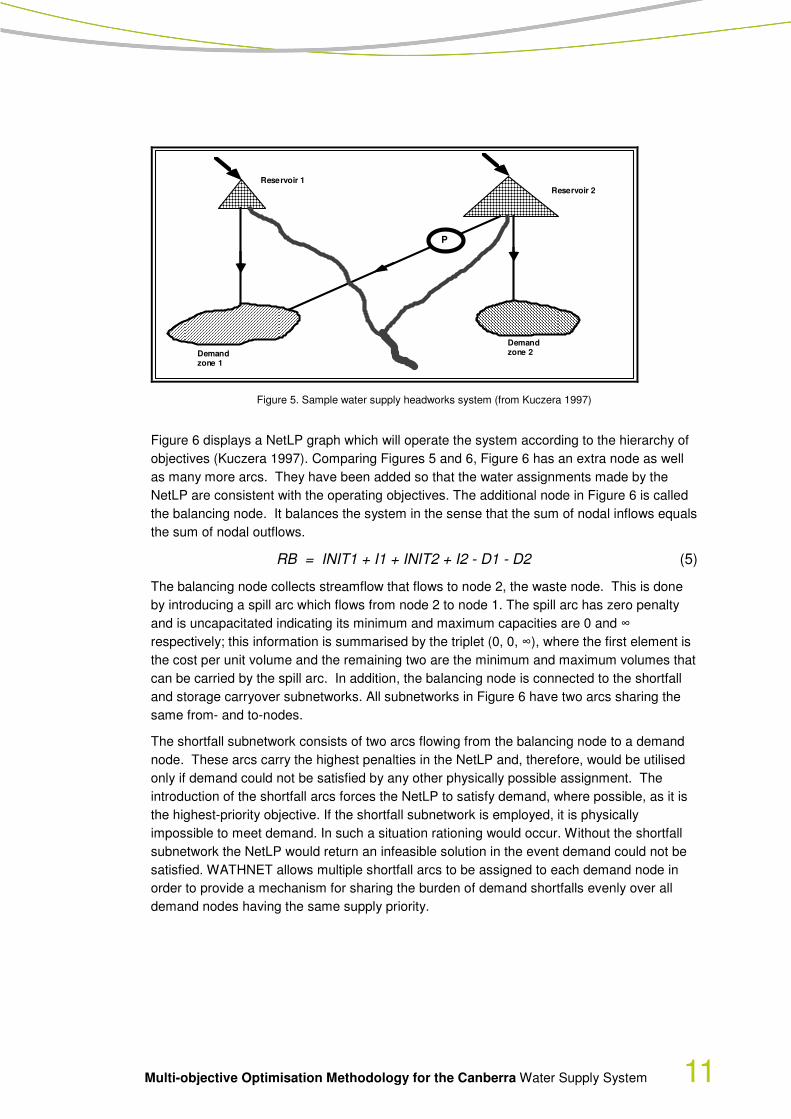
The easiest way to understand how WATHNET formulates the NetLP to solve the seasonal

water assignment problem is to illustrate it for a simple water supply system. Figure 5

(Kuczera 1997) depicts a headworks system consisting of two reservoirs with active

capacities CAPi, start-of-season volumes INITi, and inflow volumes Ii, i = 1, 2. These

reservoirs deliver water through a conduit network to two demand zones with demand

volumes Di, i = 1, 2. Water transferred from reservoir 2 to demand zone 1 must be pumped

at a unit cost of 10. All remaining conduits incur minimal delivery cost. Spills from the

reservoirs flow through downstream channels to a waste node. For both streams there is an

instream flow requirement of QMIN.


Reservoir 2

Demand zone 2Demand

zone 1

Reservoir 1

P

Figure 5. Sample water supply headworks system (from Kuczera 1997)

Figure 6 displays a NetLP graph which will operate the system according to the hierarchy of

objectives (Kuczera 1997). Comparing Figures 5 and 6, Figure 6 has an extra node as well

as many more arcs. They have been added so that the water assignments made by the

NetLP are consistent with the operating objectives. The additional node in Figure 6 is called

the balancing node. It balances the system in the sense that the sum of nodal inflows equals

the sum of nodal outflows.

RB = INIT1 + I1 + INIT2 + I2 - D1 - D2 (5)

The balancing node collects streamflow that flows to node 2, the waste node. This is done

by introducing a spill arc which flows from node 2 to node 1. The spill arc has zero penalty

and is uncapacitated indicating its minimum and maximum capacities are 0 and ∞

respectively; this information is summarised by the triplet (0, 0, ∞), where the first element is

the cost per unit volume and the remaining two are the minimum and maximum volumes that

can be carried by the spill arc. In addition, the balancing node is connected to the shortfall

and storage carryover subnetworks. All subnetworks in Figure 6 have two arcs sharing the

same from- and to-nodes.

The shortfall subnetwork consists of two arcs flowing from the balancing node to a demand

node. These arcs carry the highest penalties in the NetLP and, therefore, would be utilised

only if demand could not be satisfied by any other physically possible assignment. The

introduction of the shortfall arcs forces the NetLP to satisfy demand, where possible, as it is

the highest-priority objective. If the shortfall subnetwork is employed, it is physically

impossible to meet demand. In such a situation rationing would occur. Without the shortfall

subnetwork the NetLP would return an infeasible solution in the event demand could not be

satisfied. WATHNET allows multiple shortfall arcs to be assigned to each demand node in

order to provide a mechanism for sharing the burden of demand shortfalls evenly over all

demand nodes having the same supply priority.


2

63

4 5

1

Instream

Arcs

Instream

Arcs

W aste

Node

Demand

Node

Demand

Node

Balancing

Node

RB

Inflow

+

Initial

Storage

Inflow

+

Initial

Storage

Shortfall

Arcs

Storage

Carryover

Arcs

Figure 6. Graph of NetLP for sample water supply headworks system from Figure 4.

The instream subnetwork is introduced for every stream arc that has a non-zero instream

flow requirement. The subnetwork employs two arcs. The first arc has the parameter triplet

(-1000000, 0, QMIN), while the second has (0, 0, ∞). Because the first arc has a negative

penalty, the NetLP will try to fully utilise it to minimise the objective function. The absolute

value of the penalty is less than the shortfall penalties, but greater than any other penalties in

the NetLP. Therefore, the NetLP will make satisfying instream flow requirements its second

highest priority.

The storage carryover subnetwork consists of arcs flowing from reservoir nodes to the

balancing node, which can be thought of as a sink collecting all streamflow out of the system

as well as water carried over to the next season – the NetLP cannot store water at nodes.

Consider the reservoir at node 5 in Figure 5, the seasonal mass balance for the reservoir is

given by

Initial storage + Inflow = Release to demand nodes 3 and 6 +

Spill to waste node 2 + Final storage (6)

The initial storage and inflow are represented by the nodal requirement. At least two

carryover arcs are required for each reservoir. The first arc, the target arc, encourages the

NetLP to store water in the reservoir up to its target volume, if possible. This is accomplished

by setting a negative penalty whose absolute value is selected so that it is only exceeded by

shortfall and instream penalties. The above-target arc conveys storage in excess of the

target volume to the balancing node. However, because it has a small positive penalty, the

NetLP has no incentive to store in excess of the target volume. WATHNET allows multiple

target arcs to be assigned to each reservoir node to balance the volumes of reservoirs

having the same filling priority. Thus reservoirs with filling priority 1 will be filled in preference

to reservoirs with a lower filling priority; and, conversely, reservoirs with a priority greater


than 1 will be drawn down in preference to reservoirs with priority 1. It is noted that the user

can override this hierarchy by assigning custom penalties to the subnetworks.

3.3 Example of Network Operation

Figure 7 depicts the system during a drought and displays the assignments made by the

NetLP. Reservoirs 1 and 2 have capacities of 600 and 350 units respectively, end-of-season

target volumes of 500 and 300 respectively, and both have a filling priority of 1. Both

demand nodes have the same supply priority, namely 1.

The initial storage and inflow to reservoirs 1 and 2 are 70 and 50 units respectively.

Demands D1 and D2 are 150 and 100 units respectively. Clearly there is insufficient water

to meet demand. Therefore, an inflow of 130 units is required at the balancing node to

balance the system. This inflow is conveyed through the shortfall arcs to ensure a mass

balance at nodes 3 and 6, resulting in a demand shortfall of 80 and 50 units respectively.

Observe that the instream flow requirements were not satisfied because the higher shortfall

penalties forced the NetLP to divert all available water to the demand nodes. Also note that

both reservoirs have zero flow in their carryover sub-networks meaning their end-of-season

volumes are zero.

Figure 7. Example of a demand shortfall due to water shortage

3.4 Description of the WATHNET Program

The version of WATHNET used in this case study was adapted from the full version. The

adaptation involved consolidating and simplifying WATHNET into two parts, the simulation

engine which is data file driven, and the graphical user interface which allows construction of

the network in a controlled manner and simple visualisation of the results. This architecture

simplified the interfacing of WATHNET with the multi-objective search engine.

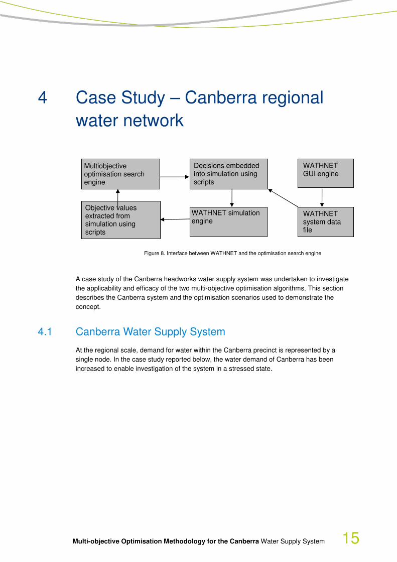
The schematic in Figure 8 describes the relationship between the WATHNET simulation

model and the optimisation engine. The WATHNET graphical user interface (GUI) engine is

used to create a network which is saved in a WATHNET data file. An important part of this

process is the use of user-written scripts. The optimisation engine implements the search for

2

6 3

4 5

1

0

0

W a s te

N o d e

5 0

0

B a la n c in g

N o d e

R B

5 0 7 0

5

0 0 0

7 0

1 3 0

0

0

0

1 0 0 1 5 0

0 0

5 0 7 5


the Pareto frontier. It passes decisions to a script which embeds the decisions in the system

configuration. WATHNET then performs the simulation. During the simulation, the user-

defined script monitors the performance of the system and calculates objective functions

values which are passed to the search engine. The search engine continues to iterate,

trialling different decision vectors until convergence has been achieved. This represents a

generic model-independent protocol for interfacing the search and simulation engines.


4 Case Study – Canberra regional

water network

A case study of the Canberra headworks water supply system was undertaken to investigate

the applicability and efficacy of the two multi-objective optimisation algorithms. This section

describes the Canberra system and the optimisation scenarios used to demonstrate the

concept.

4.1 Canberra Water Supply System

At the regional scale, demand for water within the Canberra precinct is represented by a

single node. In the case study reported below, the water demand of Canberra has been

increased to enable investigation of the system in a stressed state.

Multiobjective optimisation search engine

Decisions embedded into simulation using scripts

WATHNET simulation engine

Objective values extracted from simulation using scripts

WATHNET GUI engine

WATHNET system data file

Figure 8. Interface between WATHNET and the optimisation search engine


Figure 9. Schematic of Canberra headworks water supply system

Releases from the reservoirs have to meet, not only the consumptive needs of the Canberra

urban area, but also environmental flow requirements defined in ACTEW’s operating licence.

Downstream of each reservoir, there are several requirements based on maintenance of

base flow and pool and riffle flows. During periods of restriction, these requirements are

relaxed depending on the severity of the drought.

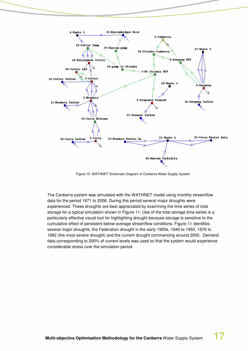
A WATHNET model of the Canberra system was constructed and is depicted in Figure 10.

The model is based on the REALM model developed by ACTEW, but has only implemented

the physical constraints affecting the system. Operating rules were not constrained as in the

ACTEW REALM model to allow the optimisation search engine maximum flexibility to search

the decision space. The ACTEW REALM model reflects rules that have been tuned to give

good performance. In this case study, the objective is to demonstrate the potential of a

generic optimisation approach to identify decisions (or rules) which lead to good

performance.


Figure 10. WATHNET Schematic Diagram of Canberra Water Supply System

The Canberra system was simulated with the WATHNET model using monthly streamflow

data for the period 1871 to 2008. During this period several major droughts were

experienced. These droughts are best appreciated by examining the time series of total

storage for a typical simulation shown in Figure 11. Use of the total storage time series is a

particularly effective visual tool for highlighting drought because storage is sensitive to the

cumulative effect of persistent below-average streamflow conditions. Figure 11 identifies

several major droughts, the Federation drought in the early 1900s, 1940 to 1950, 1976 to

1982 (the most severe drought) and the current drought commencing around 2000. Demand

data corresponding to 200% of current levels was used so that the system would experience

considerable stress over the simulation period.


Figure 11. Total storage (%) time series for a typical WATHNET simulation

4.2 Optimisation Objectives and Decision Variables

There are different objectives that can be optimised. In this study, the following three

objectives are selected to demonstrate the multi-objective optimisation methodology:

• Objective 1 (Obj1): Minimize the expected number of restrictions ( Months/year)

This objective considers the average number of months in a year that water

restrictions are required in order to meet demand and storage criteria. The objective

gives an indication of system reliability, with a lower number of months spent in water

restrictions indicating that the system has a higher level of reliability, than when water

restrictions are required often in order to meet demand.

• Objective 2 (Obj2): Minimize the expected operating cost ($/Month)

The expected operating cost of the system is the average running cost per month

calculated by dividing the total cost by the number of months of the simulation. It

involves the costs for: Pumping from Cotter and Murrumbidgee; water transferred from

Googong Dam to Googoog WTP; water transferred from Bendora to Stromlo WTP

and; water transferred from Googong WTP to Googong.

• Objective 3 (Obj3): Minimize the number of Months/year with less than 20% storage.

The average number of months per year with less than 20% storage, calculated as the

total number of months with less than 20% storage, divided by number of years in the

simulation. This gives an indication of system vulnerability to severe drought.

There are four decision variables which are summarized in Table 1.

• Decision 1: Googong base reservoir gain (BG)

0

20

40

60

80

100

120

1870 1880 1890 1900 1910 1920 1930 1940 1950 1960 1970 1980 1990 2000 2010

Year

Pere

cen

t to

tal

sto

rag

e


The base reservoir gain in Googong reservoir refers to the cost for the first storage

carryover arc from Googong reservoir. The storage carryover arcs are used to enable

setting of storage targets within the reservoirs. The cost of storage carryover arc j is

given by the following equation:

nj

IGjBGjCost

,,1

*)1()(

K=

−+= (6)

where BG is the base reservoir gain, IG is the incremental reservoir gain, and n is the

total number of storage carryover arcs. The cost of each arc affects the preference of

the system for storing water in the reservoirs, such that water is stored until it reaches

the storage target, after which, depending on the cost of the varying storage carryover

arcs, as given by the equation above, the water may be stored or spilled.

• Decision 2: Googong incremental reservoir gain (IG)

The incremental reservoir gain represents the increasing cost of each successive

storage carryover arc, such that excessive amounts of water are spilled rather than

stored. The equation for the cost of each storage carryover arc is given in equation

(6). Together with the base reservoir gain, changes in the incremental reservoir gain

essentially change the target storage in the reservoir.

• Decision 3: Canberra level 1 trigger level

The combined storage that activates the first level of water restrictions.

• Decision 4 : The restriction trigger level increment

The additional reduction in storage from a previous level which activates the next level

of water restrictions. The restriction storage trigger levels define the drought

contingency response. When total storage drops below the first trigger, restrictions on

consumption (mainly on domestic outdoor usage) are introduced and tightened as the

system draws down. The trigger levels enable hedging against failure to supply, a

state when reservoirs empty and major social and economic disruption occur.

Table 1. List of decision variables

Decision Decision variable Lower limit Upper limit

1 Googong base gain (BG) 9000 11000

2 Googong incremental gain (IG) 10 300

3 Restriction storage trigger level 1 0.1 0.9

4 Restriction trigger level increment 0.001 0.3


4.3 Performance Measures – Three Metrics

Various performance metrics for measuring the quality of a Pareto-optimal set have been

proposed to compare the performance of different multiobjective algorithms (Sarker et al.

2002). When assessing the quality of an approximate Pareto front, there are two key factors:

firstly, the proximity or closeness to the actual Pareto front, and secondly, the spread of the

obtained solutions along the front. The use of proximity or closeness is obvious, as it gives

an indication of how close the approximation is to the actual front. The spread of the

solutions along the front is desirable, as it shows a range of possible solutions, allowing a

better understanding of the true Pareto front. Metrics have been selected to assess both the

proximity and spread of the fronts found. Given that the Pareto fronts are largely unknown in

a real optimisation problem, the following metrics were used in this study.

Coverage metric – C

The coverage metric is used to assess the coverage level of one algorithm compared with

another (Zitzler et al 2000). Consider A, B as two sets of Pareto optimal solutions. The C

metric is defined as the mapping of the ordered pair (A, B) to the interval [0, 1].

{ }

B

baAaBbBAC

f:;),(

∈∃∈= (7)

where ba f means that solution dominates solution b. Therefore, C(A,B) provides the

fraction of B dominated by A. If the value C(A,B)= 1, all the decision vectors in B are

dominated by or equal to solutions in A. In contrast, C(A,B)= 0 represents the situation where

none of the points in B are dominated (covered) by A. Note that both C(A,B) and C(B,A)

have to be checked in the comparison since C-metrics are not necessarily symmetrical in

their arguments, i.e., C(A,B) = 1 - C(B,A) does not necessarily always hold.

This concept provides the absolute comparison between the Pareto values obtained using

two optimisation methods. In this study, the ε-approximate Pareto set, i.e. equation (2), is

applied when comparing solutions and b. The idea is to use a set of boxes to cover the

Pareto front, where the size of such boxes is defined by a user-defined parameter (called ε).

Within each box, only one non-dominated solution can be retained.

Cover rate - CR

The cover rate can be used to estimate the spread and distribution (or diversity) of a Pareto

set in objective space. Because the Pareto-optimal front is unknown for our targeted

application, the best possible range, the minimum (minV) and maximum (maxV) value for

each objective function, is identified by all search methods. Then for the kth objective, its

range is divided into a number of portions, with each portion equal to (maxV- minV)/N, where

N is the number of partitions. Ideally each portion can be occupied by only one solution. The

cover rate CR is defined as the percentage of the number of partitions that is covered by a

Pareto set to the total number of partitions.

For the kth objective function, the cover rate ( ) can be calculated as:

mkN

NC k

k ...1== (8)


where Nk is the number of covered partitions. Therefore, for m objective functions, the cover

rate CR can be obtained by averaging the cover rates kC for each objective function. The

desired cover rate value is 1, which indicates a wider spread and more even distribution over

the Pareto front.

Hypervolume Measure – Hv

The hypervolume measure is a unary measure which can measure the hypervolume of

objective space that is weakly dominated by the approximate Pareto set in question. If there

is no bounding on the objective space then it is calculated as the enclosed hypervolume

between a reference point and the approximate Pareto set under consideration. Figure 12

shows the hypervolume measure for a two dimensional space with three solutions (x1, x2, x3)

and reference point r. Each solution contributes a shaded rectangle, as shown, to the overall

volume. Where these volumes overlap, the overlapped area is only counted once. Using this

measure, a set with greater diversity of solutions will result in a larger Hv, as will a set which

is closer to the defined objectives, and hence closer to the Pareto front (there being no

solutions that lie beyond the Pareto front). This allows assessment based on the criteria of

proximity and spread of solutions.

The hypervolume measure is a Pareto compliant measure, meaning that given two sets A

and B, a preference for set A based on the hypervolume measure implies that the preferred

set weakly dominates (i.e. every member of set B is weakly dominated by at least one

member of set A) the other, and as such set B can conclusively be determined not to be

better than set A. The hypervolume measure is the only unary measure known to be capable

of making this assessment (Knowles et al. 2006).

4.4 Results and Discussion

In this study, the εMOGA is parameterized according to the most commonly recommended

settings from the literature (Deb et al. 2003). The probabilities of crossover and mutation

were set to Pcross=0.9, Pmutate= 0.05, respectively and the population size was assigned a

value of 100. The εMOGA stops if it reaches 10000 evaluations. The ε values for the objF1,

X1

X2

X3

r

Figure 12. The Hv for a Pareto set containing 3 solutions


objF2, objF3 are assigned values of 0.001, 100, 0.001 respectively for bounding the size of

the archive.

NSGAII has been parameterised such that it also finishes at 10000 evaluations, by setting a

population size of 100 to run for 100 generations. In this study binary encoding of the

chromosomes is used with a 16 bit string length. The probability of crossover is set to 0.9, as

with εMOGA, and the probability of mutation is set at:

l

Pm

1=

where l is the chromosome length, as recommended by Deb et al. (2002).

Case 1

Case 1 optimises two objectives; cost and the time spent in water restrictions, by changing

two decision variables; the Googong base reservoir gain and the Googong incremental

reservoir gain. These two decision variables essentially govern the drawdown policy for

operating the Googong and Corin reservoirs. Since the base and incremental gains for Corin

are fixed, varying the base and incremental gains for Googong determines whether it is the

Googong or the Corin storage that is drawn down during drought. Under optimal

management, airspace is assigned to the reservoir most likely to benefit from inflow, hence

minimizing spill from the system.

Figure 13 compares εMOGA and NSGAII fronts with the best values of the hypervolume

measure. Basically the results from two methods are quite simlar.

Figure 14 shows the εMOGA performance for every 1000 evaluations for a demand

multiplier of 200%. It is seen that after 2000 evaluations, the Pareto optimal front is

approached very quickly. This plot demonstrates that increasing the number of restrictions

will reduce operational cost.

Figure 15 shows the objective values for every member of the population every 2000

evaluations, as generated by NSGAII. While the initial population shows fairly scattered

results, with many solutions not belonging to the Pareto front, the algorithm converges

reasonably rapidly, with only minor improvements occurring after 4000 function evaluations.

This can also be seen in Figure 16 which shows the hypervolume of the population every ten

generations (or 1000 evaluations) for NSGAII. The final results obtained are similar to those

obtained using εMOGA, showing that as the time spent in water restrictions increases, the

cost of operating the system decreases. The increased amount of time in restrictions causes

a reduction in water use, and it follows that this would cause a reduction in system operating

costs.


Figure 13. Comparison of εMOGA and NSGAII fronts with the best values of the hypervolume measure

Figure 14. εMOGA performance for demand multiplier 200%

7.6 7.65 7.7 7.75 7.8 7.85 7.9 7.95 88.2

8.25

8.3

8.35

8.4

8.45

8.5

8.55

8.6

8.65

8.7x 10

5

Expected restrictions (months/year)

Cost

($/m

onth

)

NSGAII

eMOGA

815000

820000

825000

830000

835000

840000

845000

850000

855000

860000

865000

870000

7.6 7.65 7.7 7.75 7.8 7.85 7.9 7.95 8

the expected number of restrictions ( Months/year)

the e

xpecte

d o

pera

ting c

ost ($

/Month

)

Obj-initial

Obj-1000

Obj-2000

Obj-3000

Obj-4000

Obj-archive-200%


Figure 15. NSGAII results at different stages of the optimisation for demand multiplier = 200%

Figure 16. Hypervolume every ten generations for NSGAII

1 2 3 4 5 6 7 8 9 103.5

3.55

3.6

3.65

3.7

3.75

3.8

generations x 10

hyperv

olu

me


Table 2 presents three representative solutions on the Pareto front. These decisions were

selected on the basis of minimum and maximum cost and the breakpoint on the Pareto front.

What is evident is the relative insensitivity of reliability and operating cost to the way storage

is balanced between the Googong and Corin systems.

Table 2. Three solutions on Case 1 Pareto front.

Solution Googong base gain

Googong incremental gain

Restriction frequency (months/year)

Operating cost ($/month)

1 10157 17.40 7.73 832202

2 9636 10.12 7.94 822000

3 9170 152.00 7.64 864780

Case 2

Case 2 expands on Case 1. It jointly minimizes the expected time spent in water restrictions,

the expected monthly operating cost and the average number of months per year with less

than 20% storage. The last objective can be considered a measure of vulnerability to

extreme drought. In addition, Case 2 employs four decision variables: the Googong base

reservoir gain, the Googong incremental reservoir gain, the level-one restriction trigger level

and the restriction level increment. The use of four decisions enables a greater range of

system performance to be sampled.

Each of the optimisation algorithms has been parameterized such that they perform 10,000

function evaluations. For NSGAII this meant a population size of 100, which was run for 100

generations. εMOGA was run for 5000 generations, which equates to 10000 function

evaluations. Both algorithms used binary encoding, with a 16 bit string to represent the

decision variables. The probability of crossover used by NSGAII is 0.9, and the probability of

mutation is set to 0.0625. Both algorithms have then been repeated ten times using different

starting random number seeds to account for the stochasticity of the search method.

Figure 17 compares the Pareto front found by NSGA II and eMOGA after 10,000 function

evaluations. From a practical perspective there is little difference between the Pareto fronts,

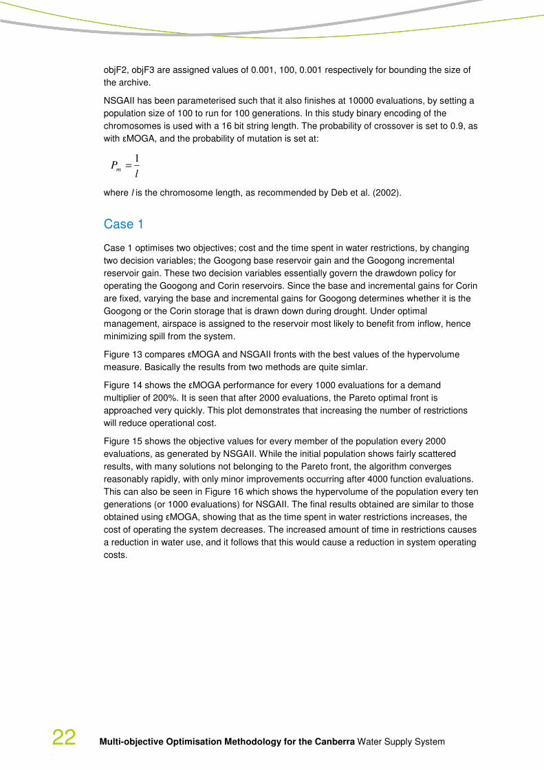
however there is some variation in the rate of convergence. Figure 18 shows the solutions

obtained every 2000 function evaluations (or 20 generations) using NSGAII. In this case, due

to the greater number of decision variables and objectives, convergence takes slightly longer

than in Case 1. However, there is still only minor improvement in the solutions after 5000

evaluations. This is also apparent in Figure 19, which shows the hypervolume of the

population every ten generations (or 1000 evaluations).

The final Pareto front obtained by both NSGAII and eMOGA, is not a surface as expected,

but rather a narrow band. This can be seen more clearly in the two dimensional projections

shown in Figures 20 to 22, where there is very little deviation from the single line. This

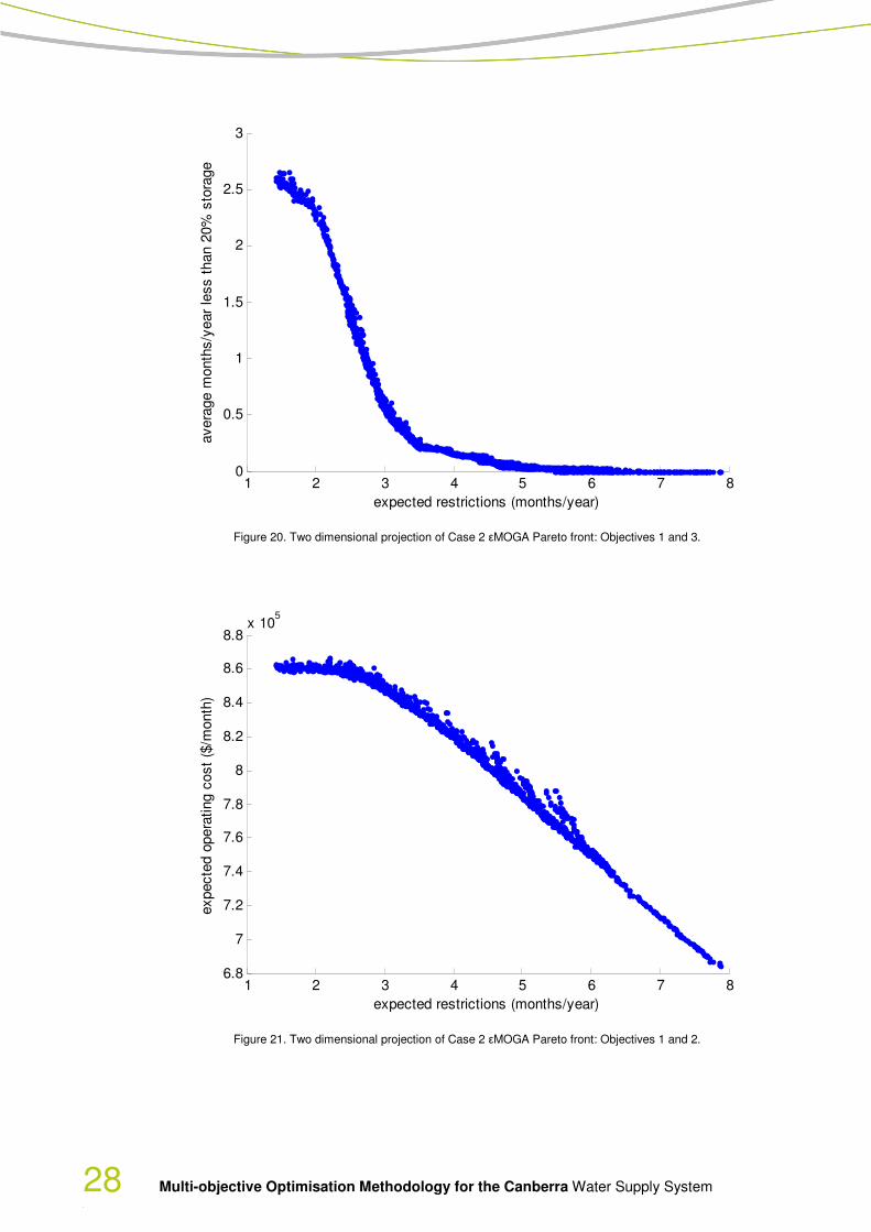
indicates that the three objectives are related to each other. Figure 20 shows an increase in

the time spent in restrictions associated with a decrease in the time with less than 20%


storage available. Figure 21 shows the operating cost decreasing as the time spent in

restrictions increases – this reflects the simple fact that consumption of water is reduced with

increased restriction frequency and therefore pumping and treatment costs are reduced.

Figure 22 shows a steep increase in the amount of time with less than 20% storage as the

cost increases. This can be accounted for by the increased operating cost of the system

when there are no water restrictions due to the increased use of water. It follows that

increased water use would cause lower storage volumes and so increase the likelihood of

total storage falling below 20%.

Figure 17. Case 2 Pareto fronts from εMOGA and NSGAII

12

34

56

78

6.5

7

7.5

8

8.5

9

x 105

0

0.5

1

1.5

2

2.5

3

expected restrictions (months/year)expected cost ($/month)

ave

rag

e m

on

ths p

er

ye

ar

with

le

ss th

an

20

% s

tora

ge

NSGAII

eMOGA


Figure 18. Case 2 NSGAII results as a function of number of evaluations.

Figure 19. Case 2 hypervolume every ten generations for NSGAII

0

2

4

6

8

10

6.5

7

7.5

8

8.5

9

x 105

0

0.05

0.1

0.15

0.2

0.25

expected restrictions (months/year)expected cost ($/month)

ave

rag

e m

on

ths/y

ea

r w

ith

le

ss th

an

20

% s

tora

ge

initial population

2000 evaluations

4000 evaluations

6000 evaluations

8000 evaluations

10000 evaluations

1 2 3 4 5 6 7 8 9 10 115.6

5.8

6

6.2

6.4

6.6

6.8

7

generations x 10

hyperv

olu

me


Figure 20. Two dimensional projection of Case 2 εMOGA Pareto front: Objectives 1 and 3.


1 2 3 4 5 6 7 80

0.5

1

1.5

2

2.5

3

expected restrictions (months/year)

avera

ge m

onth

s/y

ear

less t

han 2

0%

sto

rage

1 2 3 4 5 6 7 86.8

7

7.2

7.4

7.6

7.8

8

8.2

8.4

8.6

8.8x 10

5

expected restrictions (months/year)

expecte

d o

pera

ting c

ost

($/m

onth

)



Table 3 shows the values of decision variable associated with three different solutions from

the optimisation. One solution represents a minimization of months per year in restrictions,

one represents a minimization of cost, and the third represents the breakpoint on Figure 20,

which is indicative of a changing relationship between the number of months with less than

20% storage, and the number of months in restrictions. For the low cost solution, the storage

level at which restrictions are implemented is quite high. This indicates that restrictions are

readily imposed, resulting in a reduction in water use and hence lower system operating

costs. It should also be noted here that the only costs included are system costs and there is

no inclusion loss of income or productivity due to water restrictions.

It was found there is a strong relationship between the storage level at which restrictions are

triggered and the three objectives – see Figure 23. None of the other decision variables

show such a strong relationship with the objectives, indicating that the objectives are most

sensitive to the restriction trigger storage decision variable.

Of interest is the low value of the restriction trigger increment. In all solutions, it is at the

lower bound. Because the economic cost of restrictions is not included in the operating cost,

the optimal strategy is to impose the severest restrictions immediately. Delaying the onset of

the severest restrictions results in the Pareto inferior outcome where both expected

operating cost is higher and the chance of total storage falling below than 20% is higher.

6.8 7 7.2 7.4 7.6 7.8 8 8.2 8.4 8.6 8.8

x 105

0

0.5

1

1.5

2

2.5

3

expected operating cost ($/month)

avera

ge m

onth

s/y

ear

less t

han 2

0%

sto

rage


Table 3. Three solutions from different points on the Pareto front

Low restrictions

Breakpoint Low cost

Decision Variables

Googong base gain 10133 10526 10982

Googong incremental gain 21 54 199

Restriction storage trigger level 1 0.10 0.49 0.90

Restriction trigger level increment

0.0013 0.0011 0.0015

Objectives restrictions (months/year) 1.44 3.49 7.90

cost ($/month) 862250 835621 683478

storage less than 20% (months/year)

2.56 0.27 0.00

Figure 23. Restriction Trigger Level vs Objectives 1-3

Performance comparison

In this section, the performance of εMOGA and NSGAII are formally compared. The

population size was assigned a value of 100. Both methods were run for 10,000 evaluations.

Ten runs were performed using different random seeds, in order to account for the

stochasticity of the algorithms.

The two different optimisation algorithms, NSGAII and εMOGA, have been compared using

the three different measures outlined in Section 4.3. Table 4 shows the values of the

coverage, spacing and hypervolume metrics for the ten runs for case 1, while Table 5 shows

the same metrics for case 2. For case 1, the coverage metric shows that εMOGA performs

slightly better, since for 5 out of 10 runs, C(NSGAII, εMOGA) is less than C(εMOGA,

NSGAII). On average, 51% of εMOGA results are dominated by NSGAII while 58% of

NSGAII results are dominated by εMOGA results. This indicates that there are fewer

solutions from εMOGA which are dominated by NSGAII. The cover rate also favours εMOGA

for all 10 runs, suggesting that εMOGA can consistently produce a better spread of solutions

on the Pareto front than NSGAII.

In order to complete the comparison using the hypervolume measure, all objectives were

scaled to the interval [0,1], with the largest objective value over all runs for both optimisation

0.2 0.4 0.6 0.8

7

7.5

8

8.5

x 105

Restriction Trigger Level

Cost

($/m

onth

)

0.2 0.4 0.6 0.8

2

4

6

8


Restr

ictions (

month

s/y

ear)

0.2 0.4 0.6 0.80

1

2

3


month

s/y

ear

<20%

sto

rage


algorithms being assigned a value of 1 and the smallest being assigned a value of 0,

according to equation [9]

minmax

min

xx

xxxT

−

−= [9]

A reference point of (2,2), which is dominated by all solutions found, was selected to enable

calculation of the hypervolume. Figure 24 shows the box and whisker plots for the

hypervolumes obtained from the ten different runs for case 1 for both NSGAII and εMOGA.

The first plot is shown on an axis reflecting the likely range of variation of the hypervolumes,

while the second plot is a closer look at the variation between the two algorithms. From the

figure it can be seen that εMOGA outperforms NSGAII, although only by a small amount

given the possible amount of variation.

For case 2, coverage metric comparisons for 10 runs show similar results. In fact, Table 4

shows that C(NSGAII, εMOGA) is less than C(εMOGA, NSGAII) for all 10 runs. On average,

2.1% of εMOGA results are dominated by NSGAII while 91.1% of NSGAII are dominated by

εMOGA. The cover rate also shows similar results to those shown in Table 3.

Once again the hypervolume measure for case 2 shows that εMOGA outperforms NSGAII,

although this time by a slightly larger amount. For this case, all sets found by εMOGA weakly

dominate all sets found by NSGAII. There is a notable difference in the number of solutions

returned by NSGAII and εMOGA due to the archiving nature of the εMOGA algorithm. While

NSGAII returns a fixed number of solutions equal to the population size, εMOGA archives all

non-dominated solutions, which results in it returning between 1200 and 1300 solutions for

case 2 compared with the 100 solutions returned by NSGAII. Thus, given the nature of the

calculation it is foreseeable that εMOGA would outperform NSGAII based on the coverage

metric if both found solutions within a similar range. The advantage of returning many

solutions along the Pareto front is that there are many options for decision-makers to select

from. However, as the number of solutions provided increases, so does the difficulty of

exploring each solution. This brings into question the value of providing large numbers of

solutions, as a smaller number of solutions that are well spread along the Pareto front may

be more useful in selecting between optimal solutions. It is expected that in order to select a

final solution for implementation some form of Multi-Criteria Assessment (MCA) will be used.

In this sense it would be advantageous to have only a few solutions, which are

representative of different areas of the Pareto front. This also raises the potential advantage

of using a clustering algorithm post optimisation, in order to group similar solutions together,

which would then give an indication of representative solutions.

In short, the comparison for case 2 shows that εMOGA performs better based on the

Coverage metric and the Hypervolume metric for both the two and three objective cases.

The greater number of solutions returned by εMOGA is likely to have contributed to its better

performance based on the hypervolume measure. The sets found by NSGAII were generally

weakly dominated by those found by εMOGA, although it should be noted that overall similar

results were found.


Table 4. Comparison metrics for Case 1

Hypervolume Coverage Cover rate

εMOGA NSGAII C(NSGAII, εMOGA)

C(εMOGA, NSGAII)

S-εMOGA S-NSGAII

1 3.700 3.666 0.451 0.479 0.500 0.437

2 3.700 3.712 0.629 0.565 0.449 0.400

3 3.712 3.694 0.656 0.551 0.524 0.449

4 3.715 3.675 0.565 0.608 0.500 0.375

5 3.699 3.666 0.370 0.560 0.462 0.437

6 3.713 3.694 0.689 0.432 0.479 0.449

8 3.703 3.674 0.655 0.555 0.449 0.412

9 3.698 3.664 0.500 0.565 0.487 0.449

10 3.713 3.674 0.607 0.642 0.449 0.449

Figure 24. Box and whisker plot of hypervolumes for case 1.

3

3.1

3.2

3.3

3.4

3.5

3.6

3.7

3.8

3.9

4

NSGAII εMOGA

3.6

3.62

3.64

3.66

3.68

3.7

3.72

3.74

3.76

3.78

3.8

NSGAII εMOGA


Table 5. Performance metrics for Case 2

Hypervolume Coverage Cover rate

εMOGA NSGAII C(NSGAII, εMOGA)

C(εMOGA, NSGAII)

S-εMOGA S-NSGAII

1 6.679 6.664 0.016 0.949 0.483 0.483

2 6.700 6.644 0.032 0.930 0.491 0.466

3 6.692 6.678 0.023 0.920 0.483 0.483

4 6.704 6.647 0.021 0.920 0.483 0.483

5 6.702 6.659 0.011 0.920 0.500 0.483

6 6.679 6.646 0.017 0.839 0.483 0.483

8 6.700 6.660 0.013 0.980 0.483 0.483

9 6.700 6.657 0.035 0.920 0.483 0.474

10 6.689 6.656 0.034 0.899 0.491 0.483

Figure 25. Box and whisker plot of hypervolumes for case 2

6

6.1

6.2

6.3

6.4

6.5

6.6

6.7

6.8

6.9

7

nsga emoga

6.6

6.65

6.7

6.75

6.8

nsga emoga


5 Conclusion This study demonstrates the applicability of multi-objective optimisation methods to optimize

operating and infrastructure variables in an urban water supply headworks system. The case

study employed up to three objectives and up to four decision variables.

Ten different runs were conducted for both the NSGAII and εMOGA methods. εMOGA was

able to find slightly better Pareto fronts when compared with NSGAII, based on the

Coverage metric and the Hypervolume metric. However, the Spacing metric identified that

the solutions found by NSGAII were more evenly spaced along the Pareto front. Based on

these results, and the number of solutions returned by the algorithms, NSGAII would be

more suited to applications where fewer more evenly spread solutions are required, whereas

εMOGA is better suited to applications where a thorough characterisation of the Pareto front

is required. That said, the differences from a practical sense are small. As a result, one

would consider both methods equally capable.

This case study is of considerable practical significance as it demonstrates the power of

multi-criterion optimisation to search through trillions of possibilities and identify the

combinations of decision variables which result in Pareto dominant solutions. While the case

study only used four decision variables, subsequent studies have used many more decision

variables, confirming the generality of the approach described in this study.


6 References Coello Coello, C., Van Veldhuizen, D. A., and Lamont, G. B.: Evolutionary Algorithms for

Solving Multi-Objective Problems, Kluwer Academic Publishers, New York, 2002.

Collette, Y. and P. Siarry (2005). "Three new metrics to measure the convergence of

metaheuristics towards the Pareto frontier and the aesthetic of a set solutions in

biobjective optimisation." Comput. Oper. Res. 32(4): 773-792.

Cui, L., S. M. Mortazavi N, and G. Kuczera, Comparison of multi-objective genetic algorithm

with ant colony optimisation: a case study for Canberra water supply system

Dandekar, O. et al Multiobjective Optimisation for Reconfigurable Implementation of Medical

Image Registration, International Journal of Reconfigurable Computing, Volume 2008,

Article ID 738174, 2008.

Deb, K. Multi-objective optimisation using evolutionary algorithms. Chichester, UK: Wiley,

2001.

Deb, K., Pratap, A., Agarwal, S., and Meyarivan, T.: A Fast and Elitist Multiobjective Genetic

Algorithm: NSGA-II, IEEE Trans. Evol. Computation, 6, 182-197, 2002.

Deb, K., Mohan, M., and Mishra, S.: A Fast Multi-objective Evolutionary Algorithm for Finding

Well-Spread Pareto-Optimal Solutions, KanGAL Report No. 2003002, Indian Institute

of Technology, Kanpur, India, 2003.

Goldberg, D. E., and Kuo, C. H., Genetic algorithms in pipeline optimisation, Journal of

Computing in Civil Engineering, 1(2), April 1989.

Kennington, J. L., and Helgason, R. V., Algorithms for Network Programming, Wilsley -

Interscience, New York, 1980.

Knowles, J.D., Thiele, L. and Zitzler, E., A Tutorial on the Performance Assessment of

Stochastic Multiobjective Optimisers, TIK Report Number 214, ETH Zurich, 2006

Kuczera, G., WATHNET-Generalized Water Supply Headworks Simulation using Network

Linear Programming, Version 3, 1997.

Loucks, D. P., and Sigvaldason, O. T., Multiple reservoir operation in North America. In: The

Operation of Multiple Reservoir Systems, Z. Kaczmarek and J. Kindler (Editors), IIASA

Collaborative Proceedings Series, Laxenburg, Austria, 1982.

Laumanns, M., Thiele, L., Deb, K., and Zitzler, E.: Combining Convergence and Diversity in

Evolutionary Multiobjective Optimisation, Evol. Comput. 10, 263–282, 2002.

Reed, P., Minsker, B. S., and Goldberg, D. E.: A multiobjective approach to cost effective

long-term groundwater monitoring using an Elitist Nondominated Sorted Genetic

Algorithm with historical data, J. Hydroinformatics., 3, 71–90, 2001.

Sarker, R., Mohammadian, M., & Yao, X., eds (2002). Evolutionary Optimisation. Kluwer

Academic Publishers.


Schaffer, J. D.: Some experiments in machine learning using vector evaluated genetic

algorithms, Doctoral Thesis, Vanderbilt University, Nashville, TN, 1984.

Zitzler, E., Deb, K., and Thiele, L.: Comparison of multiobjective evolutionary algorithms:

Empirical results, Evol. Comput., 8, 125–148, 2000.

Kollat, J. B. and Reed, P. M., Comparing state-of-the-art evolutionary multi-objective

algorithms for long-term groundwater monitoring design, Advances in Water

Resources Volume 29, Issue 6, June 2006, Pages 792-807.


eWater Cooperative Research Centre

eWater Limited ABN 47 115 422 903

Innovation Centre, Building 22

University Drive South

Bruce ACT 2617

Phone: +61 2 6201 5168

[email protected]

www.ewater.com.au

eWater © 2011

20111223 Multi-objective optimisation methodology …...solution space. A Pareto optimal solution...

Documents

Transcript of 20111223 Multi-objective optimisation methodology …...solution space. A Pareto optimal solution...