20110210_ias 107
62
IAS 107 Lecture: Income- Expenditure and Investment- Savings J. Bradford DeLong U.C. Berkeley IAS107 Lecture Notes http://delong.typepad.com/berkeley_econ_101b_spring/ February 15, 2011 Resolution for screencast capture: 1024x768
-
Upload
james-delong -
Category
Documents
-
view
222 -
download
1
description
J. Bradford DeLong U.C. Berkeley IAS107 Lecture Notes http://delong.typepad.com/berkeley_econ_101b_spring/ February 15, 2011 Resolution for screencast capture: 1024x768 J. Bradford DeLong U.C. Berkeley IAS107 Lecture Notes http://delong.typepad.com/berkeley_econ_101b_spring/ February 15, 2011 Resolution for screencast capture: 1024x768 Office Hours Today 12:30-2 Tomorrow 2-4 Commercial... Problem Set 3 Due now... Please write your section time on your problem sets...
Transcript of 20110210_ias 107

IAS 107 Lecture: Income-Expenditure and Investment-
Savings J. Bradford DeLong
U.C. Berkeley IAS107 Lecture Notes
http://delong.typepad.com/berkeley_econ_101b_spring/
February 15, 2011
Resolution for screencast capture: 1024x768

Logistics: IAS 107
J. Bradford DeLong U.C. Berkeley
IAS107 Lecture Notes
http://delong.typepad.com/berkeley_econ_101b_spring/
February 15, 2011
Resolution for screencast capture: 1024x768

Today 12:30-2 Tomorrow 2-4
Office Hours

Commercial...

Due now... Please write your section time on your
problem sets...
Problem Set 3

Please write your section time on your problem sets...
Depression economics problem set due on Thursday...
<http://delong.typepad.com/berkeley_econ_101b_spring/2011/02/problem-set-4-placeholder.html>
Problem Set 4
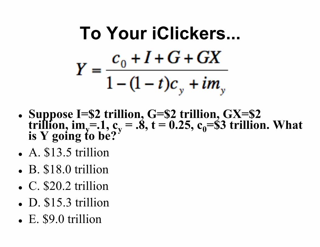
Suppose I=$2 trillion, G=$2 trillion, GX=$2 trillion, imy=.1, cy = .8, t = 0.25, c0=$3 trillion. What is Y going to be?
A. $13.5 trillion B. $18.0 trillion C. $20.2 trillion D. $15.3 trillion E. $9.0 trillion
To Your iClickers...

Answer...
€
Y =3+ 2 + 2 + 2
1− (1− t)cy + imy
Y =9
1− (1− .025)0.8 + 0.1
Y =9
1− 0.6 + 0.1=90.5
=18

For sections between Th Feb 10 @ 12:30 and Th Feb 17 @ 11:00: Skim chapters 1-5 on “securitization”: how it was that people thought that taking a whole bunch of mortgages, mashing them together, and selling the results as bonds made sense...
For sections between Th Feb 17 @ 12:30 and Th Feb 24 @ 11:00: Read chapters 6-8 on “policy”: why the American government decided at the end of the 1990s to back off of financial regulation, and let the financial sector “experiment”...
For sections between Th Feb 24 @ 12:30 and Th Mar 3 @ 11:00: Read chapters 9-15 on the bubble in subprime mortgages: how mortgage companies, banks, and investors concluded that diversified investments in even risky mortgages carried very little risk indeed...
All the Devils Are Here

For sections between Th Mar 3@ 12:30 and Th Mar 10 @ 11:00: Read chapters 16-19 on how the smart guys go short: how the more clever of the investment banks began to figure out ways to profit from the forthcoming housing crash, but how the bulk of investment and commercial bankers were not so clever...
For sections in the last week before spring break: Read chapters 20-Epilogue on the slow-motion panic that was the impulse that generated our current economic downturn...
All the Devils Are Here

Recapitulations: Things You Really Should Know
J. Bradford DeLong U.C. Berkeley
IAS107 Lecture Notes
http://delong.typepad.com/berkeley_econ_101b_spring/
February 15, 2011
Resolution for screencast capture: 1024x768

#1: You Got This

#2: You Got This...
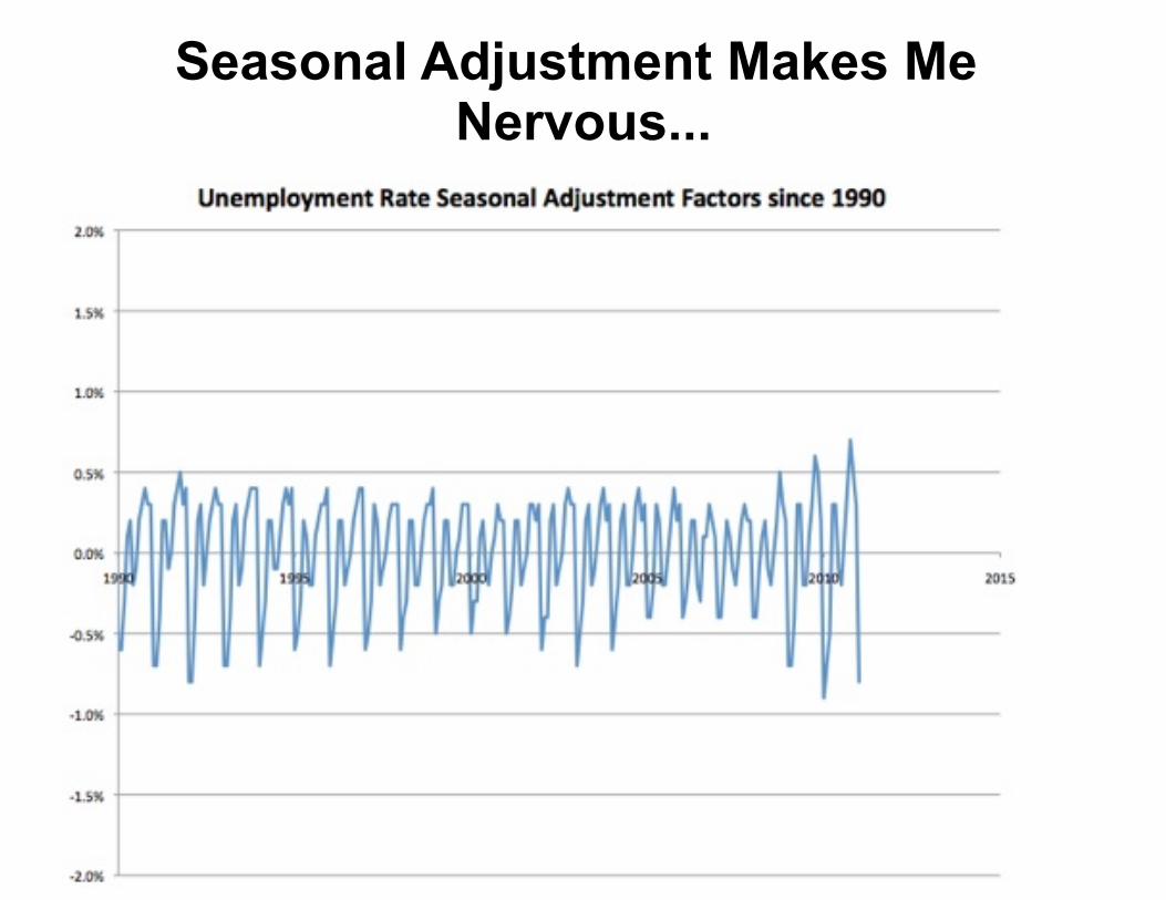
Seasonal Adjustment Makes Me Nervous...

#3: You Got This...

#4: You Got This...

#5: The Magic Equation for Depression Economics

Income-Expenditure J. Bradford DeLong
U.C. Berkeley IAS107 Lecture Notes
http://delong.typepad.com/berkeley_econ_101b_spring
February 15, 2011
Resolution for screencast capture: 1024x768

#3: You Got This...

Y = C + I + G + (GX – IM) C = c0 + cy(1-t)Y IM = imyY
The Income-Expenditure Model

Suppose I=$2 trillion, G=$2 trillion, GX=$2 trillion, imy=.267, cy = .8, t = 0.25, c0=$4 trillion. What is Y going to be?
A. $13.5 trillion B. $18.0 trillion C. $20.0 trillion D. $15.0 trillion E. $9.0 trillion
To Your iClickers...

Answer...
€
Y =c0 + I +G +GX1− (1− t)cy + imy
Y =4 + 2 + 2 + 2
1− (1− t)cy + imy
Y =10
1− (1− .025)0.8 + 0.267
Y =10
1− 0.6 + 0.267=100.667
=15

There is income on the one hand, and there is production and spending on the other
When spending is less than income and people are trying to build up their stocks of financial assets...
Businesses see their inventories rising, and fire workers...
Who lose incomes... And the process repeats... Until incomes have fallen so low that spending is
no longer less than incomes...
The Income-Expenditure Model in Words

Some Prefer Algebra

Others Prefer Graphs...

Others Prefer Graphs...

Others Prefer Graphs...
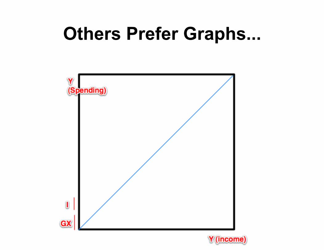
Others Prefer Graphs...
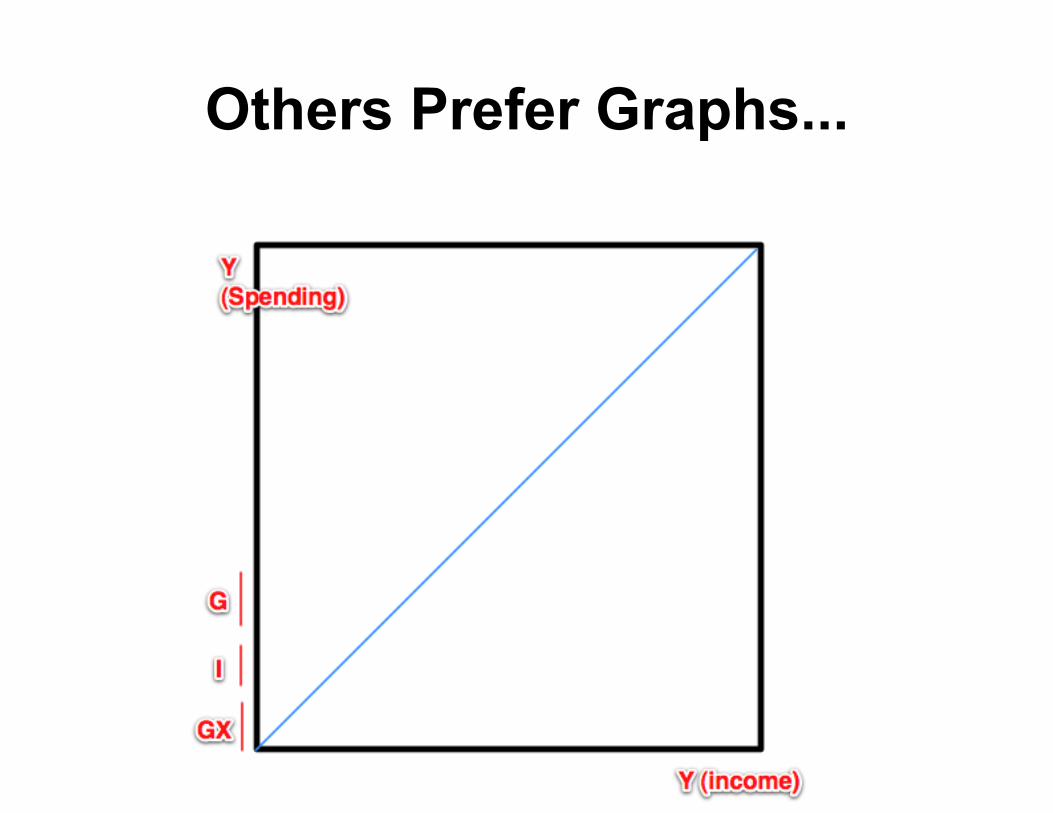
Others Prefer Graphs...

Others Prefer Graphs...

Others Prefer Graphs...

Others Prefer Graphs...

Others Prefer Graphs...

Suppose we started from the idea that there should be no excess demand for financial assets—that the flow of savings into financial markets should be equal to the number of financial assets created...
The “Excess Demand for Financial Assets” Stuff

Financial assets created: (G-T) + I Flow of savings: (Y-T-C) – NX Let us set these equal... (G-T) + I = (Y-T-C) – NX And then let’s play with it...
The “Excess Demand for Financial Assets” Stuff II

The “Excess Demand for Financial Assets” Stuff III

This is our equation for businesses being happy with what they produce—spending equal to income, no big unexpected and unwanted change in inventories
This is also our equation for no excess demand for (or supply of) financial assets
Why? Circular flow principle: as John Stuart Mill and Jean-Baptiste Say said back in 1829: an excess of demand for financial assets is a deficient demand for currently-produced goods and services
The “Excess Demand for Financial Assets” Stuff IV

Investment-Savings J. Bradford DeLong
U.C. Berkeley IAS107 Lecture Notes
http://delong.typepad.com/berkeley_econ_101b_spring
February 15, 2011
Resolution for screencast capture: 1024x768

Starting from This...

Why? So that we can have simpler formulas Simply by dropping terms that do not change
We Are Going to Look at Changes Relative to Baselines...

We Are Going to Define Autonomous Spending...
If we know the change in autonomous spending A, we know the change in income, production, output, aggregate demand, spending Y

A = c0 + G + I + GX G is determined by politics (t is too) c0 is determined by consumer confidence What determines I and GX?
And We Are Going to Go a Little Deeper...

What determines I and GX? Investment spending is determined by (a)
business confidence, and (b) the cost of capital to businesses—the long-term risky real interest rate r
Exports are determined by (a) foreigners’ incomes and (b) the real exchange rate ε
The Interest-Sensitivity of Aggregate Demand

Investment spending is determined by: (a) business confidence, and (b) the cost of capital to businesses—the long-
term risky real interest rate r ΔI = ΔI0 – Ir(Δr) Why? The higher is r, the higher is the
expected hurdle an investment project must clear for it to be profitable
Determinants of Business Investment Spending

Determinants of Business Investment Spending II

The real exchange rate—the value of the home currency—is determined by:
(a) confidence in the long-run value of the currency
(b) the difference in interest rates between home and abroad
Why? The balance between fear, optimism, and greed on the part of foreign-exchange speculators
Δε = Δε0 + εr(Δr-Δr*)
Determinants of the Real Exchange Rate

Determinants of the Real Exchange Rate II

Exports are determined by: (a) foreigners’ incomes Y*, and (b) the real exchange rate ε When foreigners are richer they buy more stuff When our stuff is more expensive foreigners
buy less of it ΔGX = Xy*(ΔY*) – Xr(Δε)
Determinants of Exports

Determinants of Exports II

ΔGX = Xy*(ΔY*) – Xr(Δε) We can substitute in our exchange rate
equation: Δε = Δε0 + εr(Δr-Δr*) To get: ΔGX = Xy*(ΔY*)-XεΔε0+Xεεr(Δr*)-Xεεr(Δr)
Determinants of Exports III

Determinants of Exports IV

ΔA = Δc0 + ΔG + ΔI + ΔGX
ΔA = Δc0 + ΔG + ΔI0 – Ir(Δr) + Xy*(ΔY*)-XεΔε0+Xεεr(Δr*)-Xεεr(Δr)
ΔA= ΔG + Δc0 + ΔI0 - XεΔε0 + Xy*(ΔY*) + Xεεr(Δr*) – [Ir+Xεεr](Δr)
Autonomous Spending Once Again

Autonomous Spending Once Again II

Now Let’s Go Back to Our Master Equation I

Suppose imy=0.1, cy=0.8, t=0.25, Ir=10, Xε=1, εr=10. Suppose that the Federal Reserve and financial markets together cut the long-term risky real interest rate r by 2%. What will happen to Y?
A. Y will rise by $0.3 trillion/year B. Y will rise by $0.6 trillion/year C. Y will rise by $0.8 trillion/year D. Y will fall by $0.6 trillion/year E. Y will fall by $0.3 trillion/year
To Your iClickers...
€
ΔY =ΔA0 + ΔG − Ir + Xεεr( )Δr
1− (1− t)cy + imy

Answer...
€
ΔY =ΔA0 + ΔG − Ir + Xεεr( )Δr
1− (1− t)cy + imy
ΔY =ΔA0 + ΔG − Ir + Xεεr( )Δr1− (1− 0.25)0.8 + 0.1
ΔY =− 10 + (1)(10)( )Δr
0.5
ΔY =− 10 + (1)(10)( )(−.02)
0.5=− 20)( )(−.02)
0.5=
+0.40.5
= 0.8

ΔY = ΔA0/[1-(1-t)cy+imy]
+ (1/[1-(1-t)cy+imy])(ΔG)
+ ([Ir+Xεεr]/[1-(1-t)cy+imy])(Δr)
And remember: ΔA0 = Δc0+ΔI0–XεΔε0+Xy*(ΔY*)+Xεεr(Δr*)
The Investment-Savings Relationship

For Those of You Who Prefer Graphs...
A0/[1-(1-t)cy+imy] + G/[1-(1-t)cy+imy]
slope = ([Ir+Xεεr]/[1-(1-t)cy+imy])

ΔY = ΔA0/[1-(1-t)cy+imy] + (1/[1-(1-t)cy+imy])(ΔG) + ([Ir+Xεεr]/[1-(1-t)cy+imy])(Δr)
Foreigners and confidence will pick out a point on the x-axis...
Fiscal policy will shift the IS curve left or right from that point on the x-axis...
Monetary policy and financial markets give you a real interest rate that picks out a point on the IS curve...
And that tells you what the level of icnome and spending in the economy is...
Using the IS Curve

“IS” stands for “Investment-Savings”... Curve first drawn by John Hicks back in... 1937, I think... It tells us at what combinations of (real, risky, long-term)
interest rates and aggregate demand levels is there neither excess nor deficient demand for “bonds”—for savings vehicles
When you are on the IS curve, there is neither deficient nor excess demand for the financial assets that are “bonds”—savings vehicles
And hence neither excess nor deficient demand for currently-produced goods and services as a whole is pushing production up or down...
If you aren’t on the IS curve, production is either rising or falling and you are heading for a position on the IS curve quickly
Why Is It Called “IS”?

Suppose imy=0.117, cy=0.6, t=0.25, Ir=10, Xε=0.5, εr=10. Suppose that the Federal Reserve and financial markets together raise the long-term risky real interest rate r by 2%. What will happen to Y?
A. Y will rise by $0.3 trillion/year B. Y will rise by $0.6 trillion/year C. Y will rise by $0.45 trillion/year D. Y will fall by $0.45 trillion/year E. Y will fall by $0.3 trillion/year
To Your iClickers...
€
ΔY =ΔA0 + ΔG − Ir + Xεεr( )Δr
1− (1− t)cy + imy

Answer...
€
ΔY =ΔA0 + ΔG − Ir + Xεεr( )Δr
1− (1− t)cy + imy
ΔY =ΔA0 + ΔG − Ir + Xεεr( )Δr1− (1− 0.25)0.6 + 0.117
ΔY =− 10 + (0.5)(10)( )Δr
0.667
ΔY =− 10 + (0.5)(10)( )(+.02)
0.667=− 15)( )(+.02)0.667
=−0.30.667
= −0.45