CERN- ATS-Note-2012-006 TECH

2012-01-19

gerard.willering@cern.ch

EDMS no: 1180914

A&T Sector Note

G.P. Willering, M. Bajko, N. Bourcey, L. Bottura, M. Charrondiere, M. Cerqueira Bastos, G. Deferne,

G. Dib, C. Giloux, L. Grand-Clement, S. Heck, G. Hudson, D. Kudryavtsev, P. Perret, M. Pozzobon,

H. Prin, C. Scheuerlein, A. Rijllart, S. Triquet, A.P. Verweij.

ELECTRO-THERMAL AND MECHANICAL VALIDATION EXPERIMENT ON

THE LHC MAIN BUSBAR SPLICE CONSOLIDATION

Acknowledgement: Task Force LHC Splices Consolidation

Summary

To eliminate the risk of thermal runaways in LHC interconnections a consolidation by placing shunts on

the main bus bar interconnections is proposed by the Task Force Splices Consolidation. To validate the

design two special SSS magnet spares are placed on a test bench in SM-18 to measure the

interconnection in between with conditions as close as possible to the LHC conditions. Two dipole

interconnections are instrumented and prepared with worst-case-conditions to study the thermo-electric

stability limits. Two quadrupole interconnections are instrumented and prepared for studying the effect

of current cycling on the mechanical stability of the consolidation design. All 4 shunted interconnections

showed very stable behaviour, well beyond the LHC design current cycle.

Electro-thermal and mechanical validation experiment on the LHC main bus bar splice consolidation

Contents Electro-thermal and mechanical Validation experiment on the LHC main bus bar splice consolidation .......... 2

1 Introduction ..................................................................................................................................................................................... 4

2 Consolidation design .................................................................................................................................................................... 5

2.1 Current LHC consolidation design ................................................................................................................................ 5

2.2 Shunt consolidation design in the experiment ........................................................................................................ 6

3 Experimental setup ....................................................................................................................................................................... 7

3.1 Cold masses and bus bars ................................................................................................................................................. 7

3.2 Instrumentation .................................................................................................................................................................. 10

3.2.1 Voltage taps ................................................................................................................................................................. 10

3.2.2 Heaters .......................................................................................................................................................................... 11

3.2.3 Temperature probes ............................................................................................................................................... 12

3.3 Defect and shunt preparation ....................................................................................................................................... 12

4 Resistance measurements ........................................................................................................................................................ 13

4.1 Resistance at room temperature ................................................................................................................................. 13

4.2 Resistance at 80 K .............................................................................................................................................................. 14

4.3 Resistance at 10 K .............................................................................................................................................................. 14

5 Thermal runaway experiments ............................................................................................................................................. 15

5.1 Typical measurement sequence and voltage interpretation ........................................................................... 15

5.2 Exponential decay at 13 and 14 kA at 1.9 K. ........................................................................................................... 18

5.3 Constant current runs at 1.9 and 4.5 K ..................................................................................................................... 19

6 Quench propagation velocity .................................................................................................................................................. 23

Example ................................................................................................................................................................................................ 23

Measurements.................................................................................................................................................................................... 24

7 Comparison between the thermo-electrical model and measurements............................................................... 25

7.1 Case 1: T = 1.9 K, I = 14 kA.............................................................................................................................................. 26

7.2 Case 2: T = 1.9 K, I = 13 kA.............................................................................................................................................. 27

7.3 Discussion on simulation results ................................................................................................................................. 28

8 Effect of current and temperature cycling ........................................................................................................................ 29

9 Further analysis and discussion ............................................................................................................................................ 29

9.1 Comparison with FRESCA measurements ............................................................................................................... 29

9.2 Value of measurements for LHC safe operation .................................................................................................... 30

9.3 Conclusions ........................................................................................................................................................................... 31

10 Bibliography .............................................................................................................................................................................. 31

Appendix A. Geometrical positions of bus bars, temperature probes, voltage taps and interconnections. 33

Appendix B. Values of all resistance measurements. ...................................................................................................... 34

Appendix C. Photo report of the experiments ................................................................................................................... 36

1 Introduction

HE incident in the LHC in September 2008 occurred in an interconnection between two magnets of the 13 kA dipole circuit [1]. It delayed the Large Hadron Collider (LHC) operation at CERN for more than

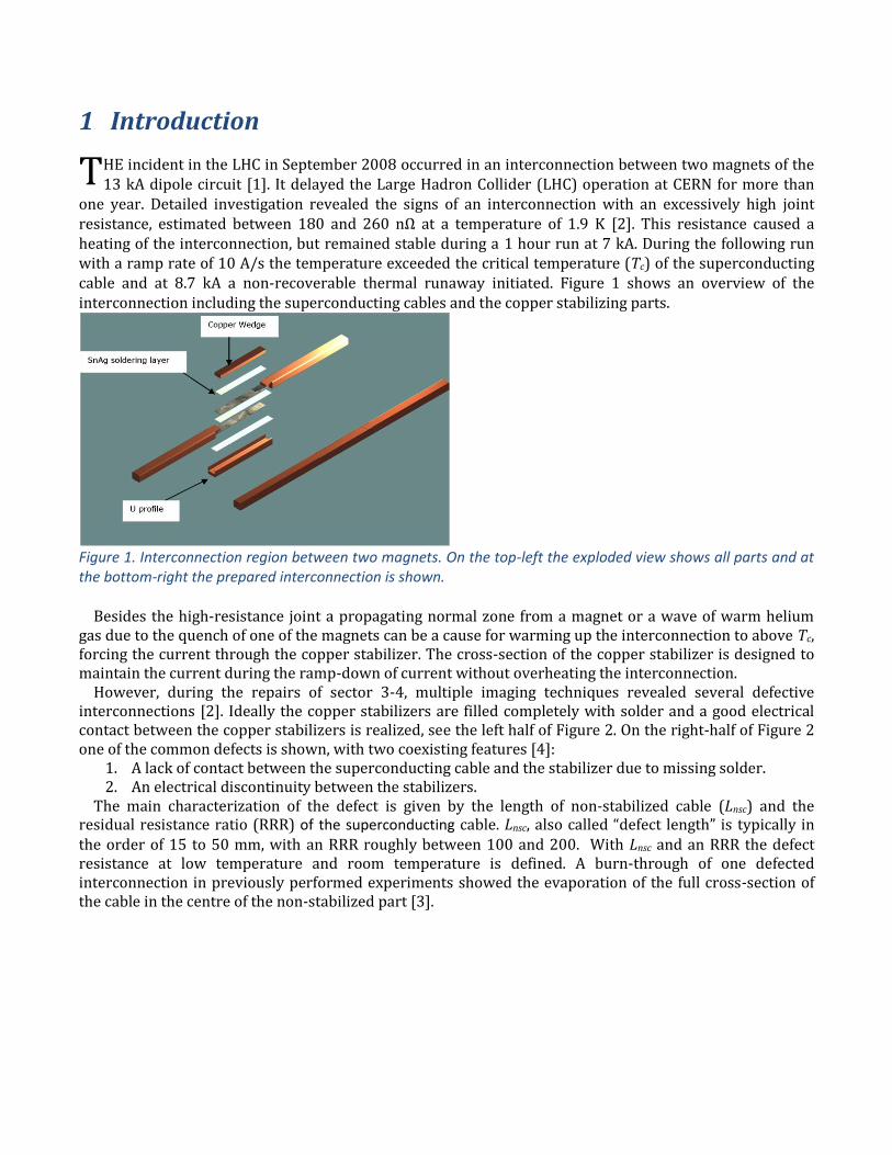
one year. Detailed investigation revealed the signs of an interconnection with an excessively high joint resistance, estimated between 180 and 260 nΩ at a temperature of 1.9 K [2]. This resistance caused a heating of the interconnection, but remained stable during a 1 hour run at 7 kA. During the following run with a ramp rate of 10 A/s the temperature exceeded the critical temperature (Tc) of the superconducting cable and at 8.7 kA a non-recoverable thermal runaway initiated. Figure 1 shows an overview of the interconnection including the superconducting cables and the copper stabilizing parts.

Figure 1. Interconnection region between two magnets. On the top-left the exploded view shows all parts and at the bottom-right the prepared interconnection is shown.

Besides the high-resistance joint a propagating normal zone from a magnet or a wave of warm helium gas due to the quench of one of the magnets can be a cause for warming up the interconnection to above Tc, forcing the current through the copper stabilizer. The cross-section of the copper stabilizer is designed to maintain the current during the ramp-down of current without overheating the interconnection.

However, during the repairs of sector 3-4, multiple imaging techniques revealed several defective interconnections [2]. Ideally the copper stabilizers are filled completely with solder and a good electrical contact between the copper stabilizers is realized, see the left half of Figure 2. On the right-half of Figure 2 one of the common defects is shown, with two coexisting features [4]:

1. A lack of contact between the superconducting cable and the stabilizer due to missing solder. 2. An electrical discontinuity between the stabilizers.

The main characterization of the defect is given by the length of non-stabilized cable (Lnsc) and the residual resistance ratio (RRR) of the superconducting cable. Lnsc, also called “defect length” is typically in the order of 15 to 50 mm, with an RRR roughly between 100 and 200. With Lnsc and an RRR the defect resistance at low temperature and room temperature is defined. A burn-through of one defected interconnection in previously performed experiments showed the evaporation of the full cross-section of the cable in the centre of the non-stabilized part [3].

T

Figure 2. Schematic drawing of an LHC splice with a single defect on the right-hand side of the interconnection.

The modelling of this problem led to a risk analysis and a decision for (i) the LHC operation [4] and for (ii) the LHC consolidation schedule [3]. The computer code [7] that provided these data is already validated by numerous thermal runaway measurements on defected as well as shunted quadrupole bus bar splices performed in the test station FRESCA [5].

The task force “LHC splices consolidation” has recommended shunting all the main LHC splices during

the consolidation in 2012 [7] after a final validation of the design. Since the test station FRESCA has a limited length and no possibilities for testing the more critical dipole interconnections, only a proof of principle test of the shunts is conducted. In a new test setup in the SM-18 test facility, 7.6 to 9 meter long bus bars are connected in an interconnect geometry which is identical to the LHC, where all test have been performed between October 2010 and January 2011.

The objective of the experiment in SM-18 on two shunted main dipole interconnections and two shunted main quadrupole interconnections is to investigate the thermo-electrical and mechanical stability of the consolidation design in real magnet to magnet connections and to validate the consolidation design.

In section 2 the LHC consolidation design is discussed. Section 3 gives an overview on the experimental condition, while section 4 goes into more details on resistance measurement method at various temperatures. In section 5 the thermo-electric tests on the dipole bus bar are reported and analysed. In section 6 the results of the quench propagation velocity measurements in the straight bus bar sections are shown. Section 7 gives a comparison between measurements and simulations for two cases and in section 8 the cycling test is discussed. Section 9 concludes with analysis and discussion.

2 Consolidation design This section describes the LHC consolidation design in some detail, followed by the design we choose to use in the experiment. The differences between them are discussed. The final optimized design might differ from what is reported here.

2.1 Current LHC consolidation design To safely operate the LHC to 13 kA throughout its lifetime a consolidation of the main splices interconnections by copper shunts is proposed. In the current consolidation design four shunts per RB interconnection (two on the top-side and two on the bottom-side) and two shunts per RQ interconnection (only on the bottom side) are foreseen. The electrical insulation in between two neighbouring RB interconnections and in between the RQ interconnections and the 600 A circuit is realized in the LHC by Polyimide wrapping and G10 pieces. In the consolidation this insulation is replaced by a special Ryton® clamp that also gives mechanical stability that needs to keep the copper pieces together in case the solder of the interconnection is melted. In Figure 3 the positioning of all insulation pieces is schematically shown.

Figure 3. An overview of the installation of a) shunts, b) centre insulation piece, c) main Ryton insulation pieces, d) all pieces installed and e) a Polyimide foil around the assembly. In f) the cross-section is shown.

2.2 Shunt consolidation design in the experiment

Shunts

In the experiment the focus is on the worst case scenario. Since there are two shunts placed for redundancy, a single shunt per connection side should allow safe operation up to 13 kA. During the experiments shunts are only placed on the top-side (worst condition) of the RB interconnections (4 in total) and on the bottom side of the RQ interconnections (4 in total).

Insulation

In the design as shown in Figure 3 the centre part of the interconnection, including the shunts, are left without further insulation wrapping to allow good cooling from the bath of superfluid helium. In the experiment the bus bar is wrapped with a double layer of 50 % overlapping Polyimide tape, thus limiting

b) a)

c) d)

e) f)

the cooling by helium. By doing so, the experiment is closer to a worst-case semi-adiabatic scenario with just He-gas around the interconnection.

Clamps

To ensure high breakthrough voltage between the bus bars and to ground, insulation clamp pieces are installed in the experiment similar to the design in Figure 3.

3 Experimental setup

3.1 Cold masses and bus bars For the test setup two options were considered:

1. Constructing a special setup for the test with a long cryogenic tube and a newly build bus bar or 2. Use two existing cold masses and make an interconnection in between them.

Option 1 was soon regarded as too time consuming, too difficult and giving too different conditions from an LHC interconnection. For option 2 a few important boundary conditions were considered.

To be able to force current through the superconducting bus bars for hundreds of seconds in normal conduction state the magnets could not be part of the electric system.

To avoid a normal zone to pass into the test stations superconducting current leads the bus bars subject to test could not be connected directly to the current leads.

The cold masses are spares for the LHC: no damage can be tolerated. Creating large quantities of gas needs to be avoided. Cryogenic feasibility to cool down the sample within a reasonable time after the quench. The test bench needs to be elongated and adapted, since it was never designed to hold two magnets.

Figure 4 shows a schematic drawing of the proposed electric scheme, having two magnets on the test bench. The two most important interconnections for the thermal runaway tests, the RB joint, are between the RB bus bars, which are located in the M3 line. The RB bus bars are connected to the RQ bus bars on the left-hand side of the picture with a quench stopper, formed by four lyres that gives additional cooling surface contact to the helium and reduces the normal resistance by its additional copper content. The quench stopper prevents the normal zone to propagate into the RQ bus bars in all conditions. The short circuit on the right-hand side of the RB bus bars allows the normal zone pass from one RB bus bar to the other. To complete the electric circuit the RQ bus bars are connected to the test bench with a standard solder connection.

Figure 4. Schematic drawing of the electric scheme of the bus bars in the test setup, with the bus bars shown in red. Two cold masses were found suitable and available for the test: the special SSS (short straight section) cold masses Q8 and Q9. In Table 1 the main specifications of the two cold masses are listed. Q9 is 1.4 meter longer than Q8 since it contains an additional magnet.

Table 1. Used SSS segments in the test setup.

SSS Quadrupole

Cryostat # Magnets Length (mm)

Cold mass assembly

CDD drawing number

Volume LHe (l)

Q8 6935 MQML+MCBC 8125 LMQMB/C LHCLMQ_0004 230 Q9 8335 MQMC+MQM+MCBC 9545 LMQMH/I LHCLMQ_0007 300 Figure 5 gives an impression of the position of the bus bars in the interconnection region and inside the cold mass. The used cryolines M1 and M3 are above each other; see Figure 5 a), with the RQ and RB bus bars surrounded by helium in the centre of the pipe. Inside the cold mass, see Figure 5 b), the bus bars are tightly packed, separated only by G10 and Polyimide. Here only small volumes of helium can penetrate the voids around the bus bar. The connection side and the lyre side of Q8 and Q9 are visualized in Figure 6, with the interconnections that are subject to test are between the connection side of Q8 and the lyre side of Q9.

Figure 5. a) Front view of the Q8 at the connection side with the M1, M2 and M3 lines indicated and b) the cross-section of a cold mass in the Q8 with the RQ- and RB-circuit bus bars (going through the M1, M2 and M3 lines) indicated.

Figure 6. a) Connection side and b) lyre side of the SSS Q8 and Q9.

b) a)

The full magnet assembly of the two magnets in Q8 and the three magnets in Q9 are shown in Figure 7. The position of the magnets is important, since the cooling of the bus bar is very different between the part of bus bars clamped inside the magnets and the part of the bus bars in the M1 and M3 line outside of the magnets.

Figure 7. a) Q8 and b) Q9 magnet assemblies, showing the position of the magnets inside the cold mass and the distances in mm.

The bus bars are straight for the full length of the magnets, but at the connection side it incorporates a bend and a fix point between the straight section and the interconnection, while the lyre side incorporates a lyre between the straight section and the interconnection, see Figure 8. Forces due to thermal contraction of the bus bar during a cool down are limited by the flexible lyre, with ∆L/L for Cu of about 0.3 % from 300 K to 1.9 K. Both the lyre and the fix point influence the quench propagation, see Section 6.

Figure 8. RB bus bar geometry in a) the Q8 cold mass and b) the Q9 cold mass with indicated lengths in mm.

3.2 Instrumentation Three types of instrumentation are implemented:

Voltage taps measure the joint and bus bar resistance at warm and during cool down and to show the development of the normal zone.

Thermocouple temperature probes are inserted in the 4 shunts on the RB interconnection to measure the temperature variations

Heaters are attached to the U-profile of the RB interconnections to provoke the start of a normal zone

3.2.1 Voltage taps In Figure 9 the position of the voltage taps, which are connected with screws, are shown. Note that V7, V16, V18 and V26 were not assembled due to the lack of space. In Appendix A the length between the voltage tap between each measured voltage tap pair is listed. The following voltage tap pairs are used for an accurate measurement of the resistance and RRR of the copper bus bar parts: RQ bus bar V1-V2, V4-V5, V28-V29, V30-V31 RB bus bar V6-V8, V15-V18, V25-V27 RQ interconnection V2-V3, V3-V4, V29-V30, V30-V31 (note: this includes a solder connection) RB shunts V9-V10, V13-V14, V19-V20, V23-V24 U-profile RB V11-V12, V21-V22

a)

b)

Figure 9. Drawing of the positioning of voltage taps V1 to V32 and temperature probes T1 to T4. The top image shows the global image with the voltage taps on the RQ bus bars and on the far ends of the bus bars. The bottom image shows a zoom of the interconnection region of the RB bus bars.

3.2.2 Heaters Commercially available flat flexible heaters are fixed at room temperature by its adhesive backing to the U-profiles in the interconnections. To ensure fixation at cryogenic temperatures and to reduce the heat loss to liquid helium around the bus bar multiple layers of Polyimide insulation are tightly wrapped around. For redundancy and for having sufficient power available to reach the critical temperature in the RB interconnections, three heaters are applied per interconnection. For the RQ interconnections less heat is required and only one heater is applied. In Table 2 the specifications of the heaters are listed and in Figure 10 a schematic drawing the interconnection cross-section is given showing the position of the heaters. Table 2. Heater specifications

Position Width (mm) Length (mm) Resistance (Ω) Supplier - Type number Bottom of U-profile 19.1 127 14.1 Minco - HK5282R14.1L12B Side of the U-profile 13.5 117 13.9 Minco - HK5260R13.9L12B

Figure 10. Cross-section of an RB and RQ interconnection with heaters visualized as black strips on each side of the RB U-profile and on the bottom side of the RQ U-profile.

3.2.3 Temperature probes In the side of each shunt a 0.5 mm hole is made to fit a thermocouple during the soldering of the shunt to monitor the solder temperature, see Figure 11. The same holes are used to glue the AuFe0.07%-Chromel thermocouple with 0.005” diameter wires inside the shunt to monitor the temperature of the shunt during the low-temperature measurements. The reference temperature is measured with a calibrated Cernox in a small box submerged in the liquid helium; see Figure 42 in the appendix.

Figure 11. Photograph of shunts on the RB interconnection, with on top the screw-fixed voltage taps and in the side of the shunt the holes fitting the thermocouples indicated by black arrows.

3.3 Defect and shunt preparation A purpose made defected interconnection requires 1) a discontinuity between stabilizer bus bars and 2) a lack of contact between superconducting cable and stabilizer. To ensure 1) the U-profile and wedge are shortened to 112 (M3a) and 104 mm (M3b). This leaves a gap between wedge and bus bar of 4 to 8 mm. To fill the removed Cu parts, purpose made G10 pieces were added to avoid having a relatively large volume of helium in the interconnection. To ensure 2) Polyimide is wrapped around the cable for a length of 30 mm, see Figure 32. This procedure reduces the joint length as well to less than 90 mm. Since the solder inside the bus bar may not be complete, the non-soldered cable length is deduced from resistance measurements as described in section 4.1. In Figure 12 the geometrical positions of all the pieces in the interconnections is drawn to scale. In Table 3 the gap length and defect length are indicated.

Figure 12. Schematic drawing to scale of the M3 interconnections, with all positions measured from the centre of the interconnection in [mm]. The position of voltage taps is indicated with the dashed lines; the length of the non-stabilized cables is shown in blue; the gap length is indicated in orange; the positions of the edges of busbar and shunts are shown in grey. Table 3. Defect and gap length of M3 interconnections.

Interconnection R8 resistance without shunt R8 (µΩ)

Non-stabilized cable length (mm)

Gap length (mm)

R8 resistance with shunt (µΩ)

M3a1 65 46 5 10.1 M3a2 53 37 4 9.9 M3b1 54 38 8 10.7 M3b2 63 45 8 10.9 Initially the resistance measurement at room temperature revealed that one shunt (M3a1) was not properly soldered to the bus bar. The R8 resistance was 15.6 µΩ, about 50% higher than expected , moreover, with another qualification method called RRT-top-side [2] the resistance for one shunt solder connection exceeded the normal value by a factor of 5. After repair the shunted part has a correct R8 value as indicated in Table 3.

4 Resistance measurements To quantify the quality of an interconnection and the length of a “defect-made-on-purpose” the resistance is measured at room temperature. For the thermo-electric stability the resistance at low temperature, characterized by the Residual Resistance Ratio (RRR) is deduced. This section gives an overview of the methods used for resistance measurement. The measurement results for all methods are listed in Appendix B.

4.1 Resistance at room temperature At room temperature two methods are used:

1. R8 and R16 measurement with a so-called Megger device, see Figure 13 for the measurement principle. A four-point resistance measurement is performed over 8 and 16 cm length and this

method was and will be used for the quality control of the LHC consolidation and for quality control of the S3-4 interconnections during the repair.

2. Four-point resistance measurement using the full electrical circuit as shown in Figure 4 and the installed voltage taps. This method is the most accurate and is used to identify the RRR of the bus bars sections.

Figure 13. Measurement with at Megger device. A current of 10 A is injected in the side 0.5 cm away from the voltage taps. The voltage is measured between V+ and V- over 8 or 16 cm.

4.2 Resistance at 80 K Magnets in SM-18 as well as in the LHC are pre-cooled by a forced flow of helium gas at about 80 K. Once this temperature is reached, it gives a stable and homogeneous temperature throughout the magnet and thus provides the possibility for an intermediate resistance measurement point. During the first cool down the resistances are measured by a four-point resistance method at 83.4 K.

4.3 Resistance at 10 K A method to identify the RRR of copper stabilizer around a NbTi superconducting sample is by slowly cooling down the sample homogeneously and obtaining the resistance just before the transition to superconducting state at 9.2 K. Using the resistance at about 10 K gives a sufficiently approximation for the resistance during operation at 1.9 to 4.3 K. However, in this case with two magnets the temperature has proven to be very inhomogeneous during cool down, and regulating it to a constant temperature around 10 K is not feasible. Therefore the magnets were filled with liquid helium and cooled down completely to 4.3 K. By closing all the inlet valves the magnets slowly warmed up and from the start of the transition to fully normal conducting conditions takes about 50 minutes. From the voltage measurement of 17 channels, see Figure 14, one can easily identify the order of warm-up of the sample. The RQ bus bars in Q8 start to warm up the quickest due to its connection to the current leads. Maybe surprisingly the last to start the transition are the interconnection regions, while the bus bars on both sides are already normal conducting. Since the temperature continues to rise slowly the values for the resistance are deduced by averaging the measurement points during the first 10 minutes after the completion of the transition.

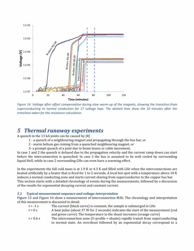
Figure 14. Voltage after offset compensation during slow warm-up of the magnets, showing the transition from superconducting to normal conduction for 17 voltage taps. The dashed lines show the 10 minutes after the transition taken for the resistance calculation.

5 Thermal runaway experiments A quench in the 13 kA joints can be caused by [8]

1 - a quench of a neighbouring magnet and propagating through the bus bar, or 2 - warm helium gas coming from a quenched neighbouring magnet, or 3- a prompt quench of a joint due to beam losses or cable movement.

In case 1 and 2 the quench is delayed due to the propagation velocity and the current ramp down can start before the interconnection is quenched. In case 3 the bus is assumed to be well cooled by surrounding liquid HeII, while in case 2 surrounding GHe can even have a warming effect. In the experiments the full cold mass is at 1.9 K or 4.3 K and filled with LHe when the interconnections are heated artificially by a heater that is fired for 1 to 2 seconds. A local hot spot with a temperature above 10 K induces a normal conducting zone and starts current sharing from superconductor to the copper bus bar. This section starts with a detailed chronology of events during the measurements, followed by a discussion of the results for exponential decaying current and constant current.

5.1 Typical measurement sequence and voltage interpretation Figure 15 and Figure 16 show a measurement of interconnection M3b. The chronology and interpretation of this measurement is discussed in detail.

t = -1 s The current (black curve) is constant, the sample is submerged in LHe t = 0 s A heat pulse (about 37 W for 2 seconds) indicates the start of the measurement (red

and green curve). The temperature in the shunt increases (orange curve) t = 0.6 s The interconnection zone (U-profile + shunts) rapidly transit from superconducting

to normal state. An overshoot followed by an exponential decay correspond to a

1.E-07

1.E-06

1.E-05

1.E-04

1.E-03

1.E-02

0 20 40 60 80 100 120

Vo

ltag

e (

V)

Time (minutes)

change of the current path from non-stabilized cable to the shunts since the redistribution is delayed by the inductance. The increase in temperature measured by the probe accelerates due to resistive heating.

t = 2.2 s The external heating is finished, only resistive heating of the sample can further increase the temperature.

t ≈ 2 - 3 s The propagating normal zone front in the Q9 direction (yellow curve) passes the Lyra. Bus bar Q9b has a resistance of 0.25 µΩ/m, corresponding to 3.6 mV/m at 14 kA, thus a level of 1.2 mV corresponds to the start of the Lyre, see Figure 8. Since the Lyra is split up in three parallel insulated parts the copper stabilizer that is in direct contact with the superconductor is smaller and therefore the resistance is bigger, resulting in a faster voltage build-up at constant velocity. While the resistance in the center part grows the current starts sharing between the three parts of the lyra, thus decelerating the voltage increase.

t > 3 s The voltage in the Q9b bus bar increases linearly, indicating a constant propagation velocity through the bus bar inside magnet filled sections of Q9.

t ≈ 3 - 12 s For the Q8 bus bar (purple curve) the average resistance is 0.22 µΩ/m, corresponding to 3.0 mV/m at 14 kA. No Lyre is present, but the propagation is reduced to almost 0 m/s at about 4 mV or equivalent to about 1.3 m. At the 1 meter mark an additional copper piece is added to the cable, slightly reducing the local resistance and giving a possibility of distortion in the insulation wrapping and adding locally cooling surface or helium volume.

t > 0.6 s The voltage in the interconnection remains constant, indicating a constant temperature in the interconnection region without signs of a thermal runaway. Also temperature sensor T4 indicates a constant temperature of 14 K.

By looking at the overall picture up to 88 seconds, see Figure 16, one can clearly identify the following events: t = 18 s Bus bar MB-Q9b reached a stable resistance of 2.6 mΩ, 20 % higher than the

resistance of the full bus bar at 10 K, indicating an average temperature in the bus bar of about 20 K.

t = 30 s The voltage increase in bus bar Q8a+b is strongly reduced, indicating a slow-down of the normal zone propagation. The voltage of 21 mV corresponds to a length of roughly 7 meter, which is about the length of the bus bar through the magnet.

t = 37 s A quick voltage increase in bus bar Q8a+b is visible, indicating the normal zone propagating into the second MB bus bar. The two neighbouring bus bars are monitored with only one voltage tapes and the two bus bars are only separated by the insulation as seen in Figure 5b inside the magnet cross-section. The quench in bus bar Q8b pre-heats bus bar Q8a. The normal zone propagation velocity is so high that this can be identified as transversal quench propagation.

t = 37 – 87 s The voltage in bus bar Q8a+b shows an accelerated increase up to 250 mV at 87 seconds when the quench protection is triggered. The resistance at 10 K of the bus bar section is 3.3 µΩ and at the moment of the quench trigger it is 5.5 times higher. This indicates a bus bar temperature of over 40 K using the assumption of uniform temperature throughout the bus bar. The hotspot temperature in the bus bar will be higher.

Bus bar Q8a shows a much less important increase in voltage.

Figure 15. Example of the measurements at I = 14 kA and T = 4.3 K following a heat pulse of 2.2 s. A fast transition to normal conduction is shown in the interconnection, quickly followed by a propagation of the normal zone in the bus bars towards Q8 and Q9.

Figure 16. Measurement signals from the same run as in Figure 15 at a constant current of 14 kA but with a zoomed out view.

5.2 Exponential decay at 13 and 14 kA at 1.9 K. The maximum LHC current rating is 13 kA and during a quench the time constant for the exponential decay in a dipole circuit is set to τ = 100 s. The performed experimental runs are listed in Table 4, showing that the tests have been performed with higher currents and time constantsTable 4. Performed runs with exponential decay at 1.9 K.. In Figure 17 the evolution of MIITs during the different runs is shown, including the test bank limit of 14 kA constant current. It is clear that during the test the MIITs are much higher than the exponential decay from 13 kA with τ = 100 s and even more significant compared to 11.85 kA with τ = 100 s (7010 106A2s). Table 4. Performed runs with exponential decay at 1.9 K.

I (kA) τ (s) MIITs (106 A2s) 13 100 8450 13 140 11830 14 100 9800 14 140 (preceded by 22 s at 14 kA constant) 18030

Figure 17. The MIITs as function of time for 5 different runs In Figure 18 the voltage measurements following heat pulses in interconnection M3b are shown for the cases listed in Table 4. In the first 3 runs, the propagation in the bus bars of Q8 is very limited and never reaches the straight section of the bus bar inside the magnet. This is explained by an increased cooling of the bus bar around the bus bar fix point, see Figure 8. The resistance in the bus bar in Q9 reduces already when the current goes down to a level below 12 or 11 kA. The interconnection region recovers relatively quickly after 22, 35, 35 and 80 seconds. One reason for the faster recovery of the interconnections is the better cooling compared to the bus bar inside the magnet.

0

2000

4000

6000

8000

10000

12000

0 10 20 30 40 50 60

MII

TS (

kA^2

s)

time (s)

11.85 kA, 100 s (7 TeV)

13 kA, 100 s (LHC design)

14 kA, 140 s

14 kA, 140 s, 22 s constant

14 kA, constant

Figure 18. Voltage following a heat pulse in interconnection M3b for a) I = 13 kA and τ =100 s, b) I = 13 kA and τ =140 s, c) I = 14 kA and τ =100 s and d) I = 14 kA for 22 seconds, followed by exponential decay with τ = 140 s.

5.3 Constant current runs at 1.9 and 4.5 K Constant current runs at 13 kA (LHC design) and 14 kA (test station limit) are performed at 1.9 and 4.5 K, see Figure 19 for an overview of relevant voltages. The following observations can be made: 1.9 K – 13 kA Very stable run. No propagation of the normal zone in the bus bars of Q8 (V15-V18). The

normal zone propagates into the bus bar of Q9 (V25-V27) but the voltage and temperature remain stable until the end of the measurement at 180 s. Also the shunt and interconnection temperature remains stable.

1.9 K – 14 kA The normal zone propagates into the bus bars of Q8, the first side is fully propagated at 31 s, while the neighbouring bus bar becomes normal at 38 s. Then the voltage continues to increase due to heating. In the bus bar of Q9 (V25-V27) the normal zone propagates faster, but the temperature remains rather constant until the neighbouring bus bar (V6-V8) also

a) b)

c) d)

becomes normal at 45 s. Why the voltage in V6-V8 is rising much quicker than in V25-V27 is not clear since they are neighboring bus bars which are expected to exchange heat. After 88 s the current is ramped to 0 A.

4.5 K – 13 kA The voltage increase is quicker than at 1.9 K – 13 and 14 kA. After 74 s the current is ramped to 0 A.

4.5 K – 14 kA The events described for the other curves happen even quicker and after 53 seconds at 14 kA Vthreshold is reached and the current is ramped to 0 A.

The induced MIITs in these runs are high: At 1.9 K – 13 kA the voltage and temperature were stable and, if the test station cooling would allow this the current could run infinitely. The total induced MIITs during these tests are listed in Table 5, which are all well above the value of the cycle at 13 kA with τ =100 s (8450 106A2s). All the runs could have lasted longer, since the maximum temperature in the circuit at cut-off of the current was always below 50 K. Table 5. MIITs induced during the tests at constant current.

Run Total time (s) MIITs (106A2s) 1.9 K – 13 kA 180 30420 1.9 K – 14 kA 88 17250 4.5 K – 13 kA 75 12675 4.5 K – 14 kA 55 10780 For comparison the voltage curves of the bus bars in Q8 (V15-V18) for the 4 runs are shown in Figure 20. By using the ρ(T) relationship of Cu and the assumption of homogeneous temperature along the normal conducting length of the bus bar the temperature is calculated. The real maximum temperature in the bus bars is higher. In Figure 21 the temperature of the bus bars is shown together with the measured temperatures of the shunts. Although the thermocouples show an absolute error, see the discussion in section 7.1, they only show a small temperature rise, but not any sign of an accelerated temperature increase, which is also indicated by the voltage measurements across the shunt. For the bus bars, in contrary, temperature starts to run away as is shown by the accelerating temperature profile. The main reason for the difference between the two is the difference in cooling for the bus bar in the magnet and the bus bar around the interconnection.

Figure 19. Measured voltages for runs with constant current. a) T = 1.9 K - 13 kA, b) 1.9 K - 14 kA, c) T = 4.5 K - 13 kA and d) 4.5 K - 14 kA.

a) b)

c) d)

Figure 20. The voltage build-up between voltage taps V15-V18 in the MB bus bars in magnet Q8 after firing heater M3B for 4 different cases of constant current.

Figure 21. Temperature profile in time of shunt M3B measured by a thermocouple (solid lines) and of the MB bus bars in magnet Q8 calculated from the voltage in V15-V18 by using the relationship ρ(T) of Cu and assuming homogeneous temperature over the bus bars. From these measurement two conclusions can be drawn:

0

50

100

150

200

250

300

0 10 20 30 40 50 60 70 80 90 100

Vo

ltag

e (

mV

)

time (s)

1.9 K - 13 kA

1. 9 K - 14 ka

4.5 K - 13 kA

4.5 K - 14 kA

0

5

10

15

20

25

30

35

40

45

50

0 10 20 30 40 50 60 70 80 90 100

Tem

pe

ratu

re (

K)

time (s)

1.9 K - 13 kA - shunt

1.9 K - 14 kA - shunt

4.5 K - 13 kA - shunt

4.5 K - 14 kA - shunt

1.9 K - 14 kA - bus bar

4.5 K - 14 kA - bus bar

4.5 K - 13 kA - bus bar

1. Submerged in superfluid or fluid helium the shunted interconnection with defect is very stable even at 4.5 K and at 14 kA for at least more than 55 seconds. The MIITs induced in the test are far higher than in the LHC at ultimate current.

2. The temperature in the bus bars shows an accelerated temperature increase before the shunted interconnections.

6 Quench propagation velocity The experiment with heaters on bus bars between magnets gives the opportunity to measure the quench propagation velocity in LHC bus bars in a real configuration inside a cold mass. In total 8 sections of bus bar are in the circuit, 4 quadrupole bus bars in line M1 and 4 dipole bus bars in line M3. Each of the 4 joints is equipped with a heater and the propagation of the quench into the bus bars in two directions is monitored.

Example After the initiation of the normal zone at t = 0 s by firing heaters, the voltage build up in the bus bars is measured, see Figure 22. The total resistance at 10 K is 3 and 3.6 µΩ for V1-V2 and V4-V28, respectively. The voltage at 12 kA is 48 and 52 mV, which is reached for both bus bars just before the quench protection kicks in. The linear slope of the curves (between 1 and 3 and 2 and 4 seconds) is used to calculate the quench propagation velocity vnzp [m/s].

Figure 22. Voltage buildup in the RQ busses next to heater M1a in cold masses Q8 (V1-V2) and Q9 (V4-V28) at a temperature of 4.5 K and a current of 12 kA.

Measurements The measured uni-directional quench propagation velocities are shown in Figure 23 and Figure 24 for quadrupole and dipole bus bars, respectively. Since the heater is positioned at the interconnection, the normal zone propagation could not be measured when the normal zone did not propagate into the straight section of the bus bar, even if vnzp > 0 m/s. In Table 6 the range of the measured quench propagation velocities is listed. A small spread between the vnzp is observed for each type of bus bar, without a clear relation to the RRR. Table 6. Range of measured quench propagation velocities for dipole and quadrupole bus bars.

Range of measured quench propagation

velocities (m/s)

Quadrupole bus bar Dipole bus bar

Current (kA) T = 1.9 K T = 4.3 K T = 1.9 K T = 4.3 K

8 0.7

9 1.0-1.1

10 0.4-0.5 1.5-1.6 0.3-0.4

11 0.5-0.8 2.1-2.4 0.5

12 1-1.3 3.1-3.3 0.7-1.0

13 1.8-2.0 0.3-0.4 1.3-1.9

14 2.8-2.9 0.4-0.7 2.5-2.9

Figure 23. Quench propagation velocity in the 4 quadrupole bus bars in M1 as function of current at both 1.9 and 4.5 K.

0

0.5

1

1.5

2

2.5

3

3.5

4

8 9 10 11 12 13 14 15 16

Pro

pag

atio

n v

elo

city

(m

/s)

I (kA)

Quadrupole bus bar

RRR 272 (1.9 K)

RRR 276 (1.9 K)

RRR 265 (1.9 K)

RRR 309 (1.9 K)

RRR 265 (4.5 K)

RRR 272 (4.5 K)

RRR 276 (4.5 K)

RRR 309 (4.5 K)

Figure 24. Quench propagation velocity in the 4 dipole bus bars in M1 as function of current at both 1.9 and 4.5 K.

7 Comparison between the thermo-electrical model and measurements

Calculations are performed with the existing computer code QP3 [6], after implementing the measurement geometry and the measured RRR of the copper stabilizers. Since creating a perfect replica of the LHC conditions is not feasible, the experiment is mainly designed to provide input and to validate the model. Decisions on the LHC collision energy are partially based on QP3 worst case scenario calculations. In this section two simulation cases are shown, compared with the experiment and followed by a discussion of the results. The main goal of the simulations is to verify the simulation program by fitting the simulation to the measurements with limited curve fitting parameters. As much parameters as possible are directly obtained from measurements, like the exact geometry of the interconnection and bus bars, the insulation around the bus bar and the RRR of the copper pieces. Free parameters that have been used to fit calculations to measurements the cases shown below are listed in Table 7. Table 7. Free parameters used for the curve fitting.

Effective polyimide tape insulation thickness – Bus and Joint 0.29 mm Effective polyimide tape insulation thickness - Shunt 0.02 mm Film boiling heat transfer coefficient 1250 W/m2/K RRR shunt 160 Helium volume around bus bar per unit length – Interconnection tube 40000 mm3/mm Helium volume around bus bar per unit length – Along magnet 260-300 mm3/mm

0

0.5

1

1.5

2

2.5

3

3.5

4

8 9 10 11 12 13 14 15 16

Pro

pag

atio

n v

elo

city

(m

/s)

I (kA)

Dipole bus bar

RRR 260 (1.9 K)

RRR 264 (1.9 K)

RRR 308 (1.9 K)

RRR 308 (1.9 K)

RRR 260 (4.5 K)

RRR 264 (4.5 K)

RRR 308 (4.5 K)

RRR 308 (4.5 K)

7.1 Case 1: T = 1.9 K, I = 14 kA. In Case 1 the interconnection is submerged in superfluid helium at 1.9 K, while the current is constant at 14 kA. In Figure 25 four simulation curves are plotted (red lines) and compared with measurements (blue lines). In Figure 25 a) the voltage across the shunt is accurate within 10 %, but it shows a small increase during the full experimental run. These small variations can be simulated by making small adapting cooling parameters well within the known parameter range. In Figure 25 b) the temperature of this shunt is shown. There is a striking resemblance between the shapes of the two curves:

- at 0.6 s an accelerated temperature increase related to the superconducting cable becoming normal conducting and additional heating starts.

- At 2.4 s the heating by the heater stops, resulting in a reduction of temperature. However, the absolute value of the simulation does not correspond to the measured value. Since the critical temperature of NbTi is 9 K, and the temperature of the shunt is at around 5 K when the sample becomes normal the temperature measured with the thermocouple is believed to be erratic, probably caused by too much contact with helium and the temperature of the thermocouple is actually lower than the shunt temperature. Figure 25 c) shows the propagation of the normal zone into the bus bar in Q9. From 0 to 18 s one can see a linear increase or a constant normal zone propagation velocity until the full bus bar between the voltage taps is normal conducting. The increase in voltage afterwards depicts a resistance increase and thus a temperature increase in the bus bar. Figure 25 d) shows the same in the direction of Q8, however here the voltage remains at a stable level of 3 mV for quite some time. The quench stops propagating at around the “fix point” just before the bus bar enters the magnet, see also Figure 8. To include this feature in the simulations the fix point was added and an assumption about a disturbance in the insulation wrapping was made.

Figure 25. Measured (solid blue) and calculated (dashed red) curves for the run at 1.9 K with a constant current of 13 kA. In a) the voltage on the shunt, in b) the temperature of the shunt measured by thermocouple T3, in c) the voltage across the bus bar in Q9 and in d) the voltage across the bus bars of Q8.

7.2 Case 2: T = 1.9 K, I = 13 kA. For case 2 the same parameters are used in the simulation as in case 1 and similarly correct results are obtained. In Figure 26 four simulation curves are plotted (red lines) and compared with measurements (blue lines). In Figure 26 a) a stable voltage is calculated and measured across the shunt, again with a 10% difference between the two. Figure 26 b) shows a similar shape of the temperature in the shunt as in case 1, although the accelerated temperature increase is not visible in the measurement. The quench propagation in bus bar Q9, see Figure 26 c), has a similar velocity in measurement and calculation, but it lags a bit behind in the calculation. With a constant current starting from 30 s, the temperature of the bus bar is stable. In Figure 26 d) the propagation of the normal zone does not reach the bus bar inside the magnets, but it remains stable once it reaches 2 mV.

0

5

10

15

20

25

30

35

40

45

50

0 20 40 60 80 100

Vo

ltag

e (m

V)

time (s)

V27-V25Busbar Q9

0

2

4

6

8

10

12

14

16

18

20

0 1 2 3 4 5

Tem

pe

ratu

re (K

)

Time (s)

T3 (shunt)

0

5

10

15

20

25

30

35

40

45

50

0 20 40 60 80 100

Vo

ltag

e (m

V)

Time (s)

V27-V25Busbar Q9

0

2

4

6

8

10

12

14

16

18

20

0 5 10 15 20 25 30

Vo

lta

ge

(mV

)

Time (s)

V18-V15Bus bars Q8

a) b)

d) c)

Figure 26. Measured (solid blue) and calculated (dashed red) curves for the run at 1.9 K with a constant current of 14 kA. In a) the voltage on the shunt, in b) the temperature of the shunt measured by thermocouple T3, in c) the voltage across the bus bar in Q9 and in d) the voltage across the bus bars of Q8.

7.3 Discussion on simulation results Overall the simulations agree very well with the measurements. The main discrepancy is the temperature of the shunt that is measured with a thermocouple. There are strong indications that the thermocouples are not showing the temperature of the shunt, but a lower one, which is probably due to contact with helium. Despite these differences all the curve characteristics are very well simulated. Fine tuning of the parameters so as to fit the measurements even better is possible, but has only a marginal effect on the calculated safe current. Both cases are calculated with the same set of parameters and re-validate the program for use in predicting safe current levels for shunted interconnections.

0

0.5

1

1.5

2

2.5

0 20 40 60 80 100

Vo

ltag

e (m

V)

Time (s)

V25-V18Shunt

0

2

4

6

8

10

12

14

16

18

20

0 1 2 3 4 5

Tem

pe

ratu

re (K

)

Time (s)

T3 (shunt)

0

5

10

15

20

25

30

35

40

45

50

0 20 40 60 80 100

Vo

ltag

e (m

V)

Time (s)

V27-V25Bus bar Q9

0

2

4

6

8

10

12

14

16

18

20

0 10 20 30 40

Vo

lta

ge

(mV

)

Time (s)

V18-V15Bus bars Q8

b) a)

d) c)

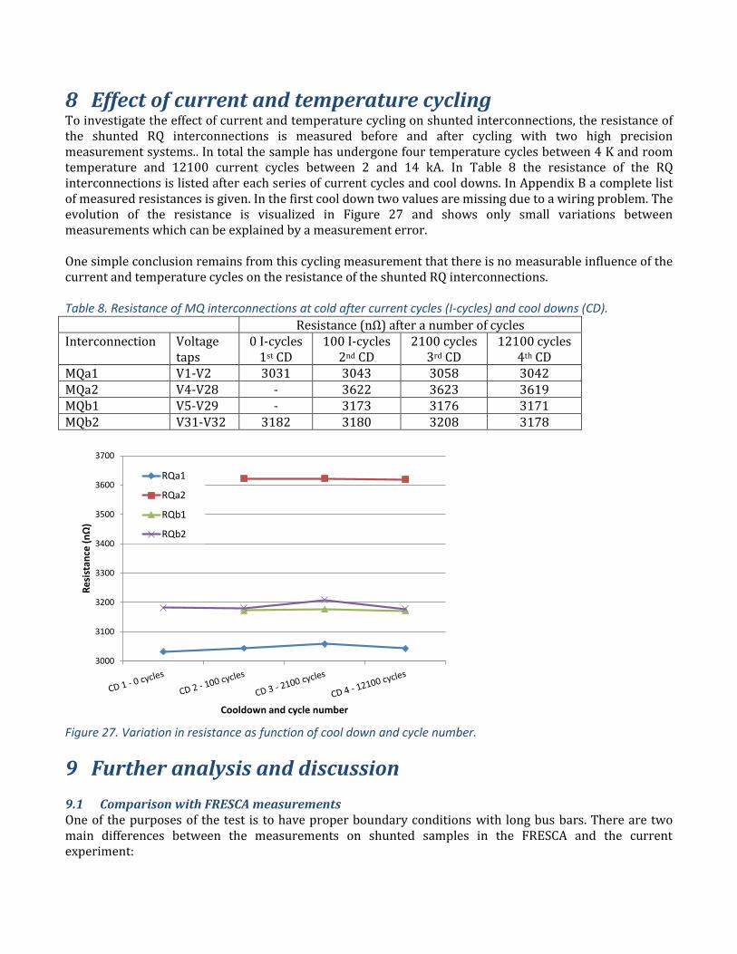
8 Effect of current and temperature cycling To investigate the effect of current and temperature cycling on shunted interconnections, the resistance of the shunted RQ interconnections is measured before and after cycling with two high precision measurement systems.. In total the sample has undergone four temperature cycles between 4 K and room temperature and 12100 current cycles between 2 and 14 kA. In Table 8 the resistance of the RQ interconnections is listed after each series of current cycles and cool downs. In Appendix B a complete list of measured resistances is given. In the first cool down two values are missing due to a wiring problem. The evolution of the resistance is visualized in Figure 27 and shows only small variations between measurements which can be explained by a measurement error. One simple conclusion remains from this cycling measurement that there is no measurable influence of the current and temperature cycles on the resistance of the shunted RQ interconnections. Table 8. Resistance of MQ interconnections at cold after current cycles (I-cycles) and cool downs (CD).

Resistance (nΩ) after a number of cycles Interconnection Voltage

taps 0 I-cycles

1st CD 100 I-cycles

2nd CD 2100 cycles

3rd CD 12100 cycles

4th CD MQa1 V1-V2 3031 3043 3058 3042 MQa2 V4-V28 - 3622 3623 3619 MQb1 V5-V29 - 3173 3176 3171 MQb2 V31-V32 3182 3180 3208 3178

Figure 27. Variation in resistance as function of cool down and cycle number.

9 Further analysis and discussion

9.1 Comparison with FRESCA measurements One of the purposes of the test is to have proper boundary conditions with long bus bars. There are two main differences between the measurements on shunted samples in the FRESCA and the current experiment:

3000

3100

3200

3300

3400

3500

3600

3700

Res

ista

nce

(nΩ

)

Cooldown and cycle number

RQa1

RQa2

RQb1

RQb2

1. The FRESCA samples where impregnated over the whole interconnection region, making it a worst case situation.

2. The bus bar during the current experiment is much longer, thus making it worse compared to the FRESCA experiment.

In Figure 28 the limiting MIITs for constant currents in the FRESCA measurements are indicated in the curves [3], with the diamond indicating the MIITs reached in the current experiment. However, the latter is not a limit, since there was not yet any sign of a thermal run-away. Hence the value is even higher than indicated. Note that the MIITs for exponential decay have less impact than for constant current, as is shown in this report.

Figure 28. The measured MIITs until the thermal runaway starts as a function of current. The lines indicate the samples measured in the test station FRESCA where the 5 curves in the bottom left are samples with only defects, no shunts. The 4 curves more to the right are shunted samples. The dashed lines indicate the MIITs in the LHC circuits with a τ of 10, 20 and 100 s. The diamond indicates the limit of the current test at which the shunt is very stable.

9.2 Value of measurements for LHC safe operation Since the experimental setup cannot replicate of LHC conditions exactly, the purpose of the test has never been determining safe operation current levels, but generating sufficient data to validate calculations by supplying conditions approaching LHC worst case conditions. In Table 9 a comparison is made between LHC worst case conditions as they are currently used for safe current calculations and the condition in the experiment. Table 9. Comparison between current LHC worst case conditions and experimental characteristics.

LHC Experiment RRR of shunt > 200 RRR of cable > 80

RRR of shunt with cable in parallel = 160 (determined for about 80 % by shunt)

RRR bus bars >180 RRR bus bars = 260 – 300 RRR U-profile > 130 RRR U-profile = 150 - 180

100

1000

10000

100000

6 8 10 12 14 16 18 20

MII

Ts

un

til

run

aw

ay

(1

06

A2s)

Current (kA)

No Polyimide insulation wrapping in the interconnection region

2 double layers of Polyimide insulation wrapping

Possibility of GHe Always LHe around the interconnection Max 13 kA, τ = 100 s Test up to 14 kA, τ = ∞. Cu-pieces of bus bar removed and replace by G10 Non-soldered shunt length < 10 mm Non-soldered shunt length 4 – 8 mm Non-stabilized cable length < 30+30 mm Non-stabilized cable length 46+37 and 38+45 mm Shunt dimension: 50 x 15 x 3 mm3 Shunt dimension: 50 x 15 x 3 mm3 An effort was made to make the measurement conditions worse than LHC conditions. This was feasible for the RRR of the shunt, the removal of Cu in the interconnection area, the non-stabilized cable length and the insulation of the interconnection. The cooling conditions for the experiment were better than in the LHC, specifically when considering a magnet quench followed by He-gas production. No (semi-)adiabatic tests could be performed on the sample. The non-soldered shunt length is guaranteed to be limited to 10 mm in the consolidation whereas in the experiment 4 to 8 mm is considered. However, applying a constant current of 14 kA is increasing the heating power in the interconnection by a large factor.

9.3 Conclusions 1. The results clearly indicate with large confidence that with these experimental conditions the

shunted interconnection was extremely stable, not showing any signs of a thermal run-away, even at 4.5 K at 14 kA for much more than 55 seconds.

2. Experimental results and simulations with the electro-thermal model QP3 are in good agreement, even with very limited curve fitting efforts. This is an additional validation of the simulation program and parameters.

3. 12100 current cycles to 14 kA and 4 thermal cycles have no measurable influence on the resistance of the shunted interconnections.

4. The feasibility of applying top shunts to RB and bottom shunts to RQ interconnections is proven on a real magnet to magnet interconnection.

10 Bibliography

[1] P. Lebrun et al., “Report of the Task Force on the Incident of 19 September 2008 at the LHC,” CERN LHC Proj. Rep. 1168, 2009.

[2] M. Bajko et al., “Report of the taskforce on the incident of 19 September 2008 at the LHC,” Geneva, Switzerland, 2009.

[3] F. Bertinelli, L. Bottura, J.-M. Dalin, P. Fessia, R. Flora, S. Heck, H. Pfeffer, C. Scheuerlein, P. Thonet, J.-P. Tock and L. Williams, “Production and Quality Assurance of Main Busbar Interconnection Splices during the LHC 2008-2009 Shutdown,” IEEE Trans. Appl. Supercond., vol. 22, no. 3, p. 1786, 2011.

[4] A. P. Verweij, “Bus bar and joints stability and protection,” Proc. Chamonix workshop on LHC Perf., 2009.

[5] G. Willering, L. Bottura, P. Fessia, C. Scheuerlein and A. Verweij, “Thermal runaways in LHC interconnections: Experiments,” IEEE Trans. Appl. Superc., vol. 21, no. 3, pp. 1781 - 1785, 2010.

[6] A. Verweij, “Thermal runaway of the 13 kA busbar joints in the LHC,” IEEE Trans. Appl. SC, vol. 20, no. 3, pp. pp. 2155-2159, 2010.

[7] A. Verweij, “Minimum requirements for the 13 kA splices for 7 TeV operation,” Chamonix 2010.

[8] A. Verweij, “QP3, Computer code for the calculation of Quench Process, Propagation, and Protection,” 2009.

[9] A. Verweij, F. Bertinelli, N. Catalan Lasheras, Z. Charifoulline, R. Denz, P. Fessia, C. Garion, H. ten Kate, M. Koratzinos, S. Mathot, A. Perin, C. Scheuerlein, S. Sgobba, J. Steckert, J.-P. Tock and G. Willering, “Consolidation of the 13 kA interconnections in the LHC for operation at 7 TeV,” in ASC 2010 conference, Washington, to be published, 2010.

[10] S. Heck, C. Scheuerlein and G. Willering, “Room temperature resistance measurements for the quality control of shunt solder connections for the consolidation of the LHC main interconnection splices,” CERN, Techical note TE-2010-34, EDMS 1097684, 2010.

[11] A. Verweij, “Probability of burn-through of defective 13 kA joints at increased energy levels,” in Proc. 2011 LHC Performance Workshop, Chamonix, january 2011, 2011.

[12] “LHC design report,” Geneve, Switzerland, 2004.

Appendix A. Geometrical positions of bus bars, temperature probes, voltage taps and interconnections.

Table 10. Geometrical positions of bus bars temperature probes, voltage taps and interconnections.

Voltage tap pair

Description Length (m)

V1-V2 MQ-Q8a 7.64 V2-V3 MQ-interconnection a1 0.080 V3-V4 MQ-interconnection a2 0.080 V4-V28 MQ-Q9a 9.04 V28-V27 ~ 0.4 V27-V25 MB-Q9a 9.4 V25-V24 0.000 V24-V23 0.030 V23-V22 0.007 V22-V21 MB-U-profile a 0.087 V21-V20 0.006 V20-V19 0.031 V19-V18 0.006 V18-V15 MB-Q8a+b 15 V15-V14 0.001 V14-V13 0.030 V13-V12 0.006 V12-V11 MB-U-profile b 0.088 V11-V10 0.009 V10-V9 0.030 V9-V8 0.001 V8-V6 MB-Q9a 9.40 V6-V5 ~ 0.4 V5-V29 MQ-Q9b 9.04 V29-V30 MQ-interconnection b1 0.080 V30-V31 MQ-interconnection b2 0.080 V31-V32 MQ-Q8b 7.64

Appendix B. Values of all resistance measurements. Table 11. Overview of resistance for all cool downs

Part type Voltage taps Resistance at 297 K

Resistance at 83.4 K

Resistance at 10 K 0 Icycles

CD 1

Resistance at 10 K 100 Icycles CD 2

Resistance at 10 K 2100 Icycles CD 3

Resistance at 10 K 12100 Icycles

CD 4 [µΩ] [µΩ] [nΩ] [nΩ] [nΩ] [nΩ]

busbar RQ V1-V2 823.2 119.2 3031 3043 3058 3042 busbar RQ V4-V28 986.2 141.9 - 3622 3623 3619 busbar RQ V5-V29 980.2 140.6 - 3173 3176 3171 busbar RQ V31-V32 824.3 119.5 3182 3180 3208 3178 MQ-interconnection V2-V3 7.8 1.148 44.22 44.33 44.82 44.33 MQ-interconnection V3-V4 8.0 1.189 - 52.73 52.42 52.60 MQ-interconnection V29-V30 7.4 1.095 - 42.91 42.98 42.95 MQ-interconnection V30-V31 8.3 1.217 46.90 47.03 46.88 46.76 busbar RB V6-V8 579.3 82.74 2238 2223 2236 2235 2*busbar RB V15-V18 1026.6 147.6 3341 3327 3344 3331 busbar RB V25-V27 577.1 82.39 - 2184 2194 2197 Shunt RB V9-V10 5.1 0.755 31.50 30.65 30.93 30.92 U-profile RB V11-V12 4.8 0.702 26.34 26.43 26.53 26.65 Shunt RB V13-V14 4.9 0.742 31.18 30.68 30.76 30.79 Shunt RB V19-V20 5.4 0.806 33.24 33.01 33.12 33.14 U-profile RB V21-V22 4.6 0.661 - 24.99 24.93 25.06 Shunt RB V23-V24 5.9 0.874 36.35 35.84 36.08 36.01 Table 12. RRR (R293K /R10K, 0T) Averaged over all cool downs and with R293K = 0.985*R297K

Part type Voltage taps RRR 2*busbar RB V15-V18 303 busbar RB V6-V8 256 busbar RB V25-V27 260 busbar RQ V1-V2 266 busbar RQ V4-V28 268 busbar RQ V5-V29 304 busbar RQ V31-V32 255 MQ-interconnection V2-V3 173 MQ-interconnection V3-V4 149 MQ-interconnection V29-V30 170 MQ-interconnection V30-V31 174 Shunt RB V9-V10 160 Shunt RB V13-V14 158 Shunt RB V19-V20 161 Shunt RB V23-V24 162 U-profile RB V11-V12 181 U-profile RB V21-V22 180

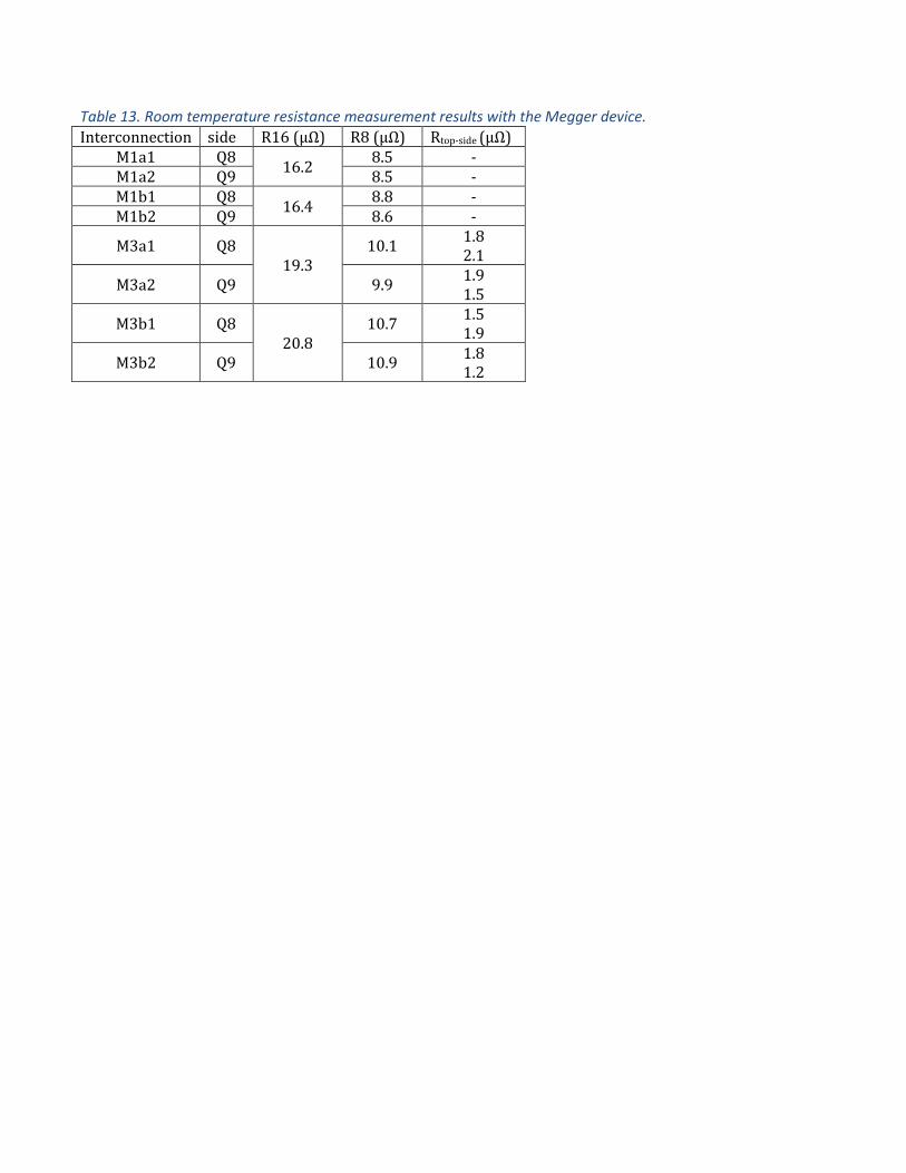
Table 13. Room temperature resistance measurement results with the Megger device.

Interconnection side R16 (µΩ) R8 (µΩ) Rtop-side (µΩ)

M1a1 Q8 16.2

8.5 - M1a2 Q9 8.5 - M1b1 Q8

16.4 8.8 -

M1b2 Q9 8.6 -

M3a1 Q8 19.3

10.1 1.8 2.1

M3a2 Q9 9.9 1.9 1.5

M3b1 Q8 20.8

10.7 1.5 1.9

M3b2 Q9 10.9 1.8 1.2

Appendix C. Photo report of the experiments

Figure 29. M1 interconnection after being machined, before the positioning of the shunt.

Figure 30. M1 interconnections as seen from the bottom side. The 4 shunts are soldered into their position.

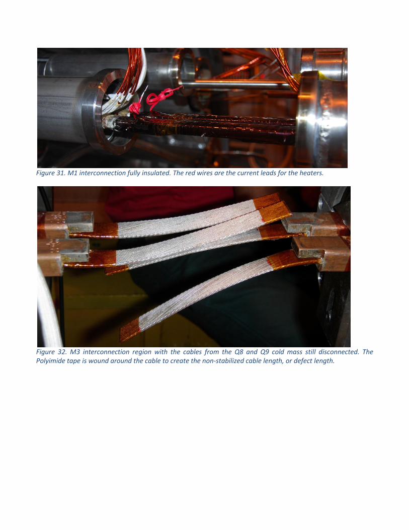
Figure 31. M1 interconnection fully insulated. The red wires are the current leads for the heaters.

Figure 32. M3 interconnection region with the cables from the Q8 and Q9 cold mass still disconnected. The Polyimide tape is wound around the cable to create the non-stabilized cable length, or defect length.

Figure 33. M3 interconnections with parts of the U-profile and wedge cut out. M3a is in front with gaps of 4 and 5 mm, M3b is in the background with two gaps of 8 mm.

Figure 34. M3 interconnection after soldering the shunts.

Figure 35. Close up of shunt 1 in interconnection M3a

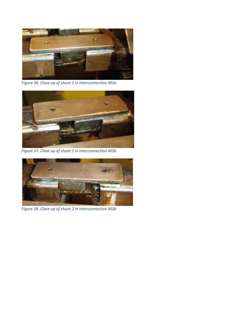
Figure 36. Close up of shunt 2 in interconnection M3a

Figure 37. Close up of shunt 1 in interconnection M3b

Figure 38. Close up of shunt 2 in interconnection M3b

Figure 39. The M3 interconnection after preparing the insulation and instrumentation.

Figure 40. The clamp box made of Ryton® is placed around the interconnection.

Figure 41. The box is covered with a Polyimide foil and fixed with tie-rips. Thermocouple wires come out of the hole the connect to the reference temperature box.

Figure 42. The reference temperature box contains a calibrated CERNOX temperature sensor and the thermocouple references are placed in this box.

Figure 43. The interconnection between Q9 and the quench stopper with the voltagetaps V6 and V27 just left of thon the end of M3 busbars in Q9. The Vtap wires are connected to the 600 A lines by passing a wire through the quench stopper box)

Figure 44. Connection box containing the quench stopper on the right with the Q9 cold mass on the left.

Figure 45. Quench stopper container after welding.

Figure 46. Quench stopper (a busbar with two soldered lyra’s to increase the heat exchange with helium). The bottom is connected to M3, the top is connected to M1.

Figure 47. Overview of the Q8-Q9 interconnection region, with the two magnets on the test bench.

Figure 48. Overview of the Q8 and Q9 positioned on the test bench

Figure 49. Q8 cryostat connection side with the instrumentation connection box welded to the M3 line

N

Connection box

M3

M2

M1

Figure 50. Connection box close-up with the all-important tube (left-bottom) to pump the chamber inside the box vacuum.

Figure 51.The voltage taps on the far ends of the cold masses (Q8 lyra side and Q9 connection side) are linked to the connection box through the 600 A lines. On the picture the wire connections are visible.