2011 ASFPM NATIONAL CONFERENCE

Plenary and Concurrent Session Presentations

By presenting at the 2011 ASFPM Annual National Conference, presenters authorized ASFPM to display, show, and redistribute, without alteration, the presentation materials provided for use at the 2011 ASFPM Annual National Conference. ASFPM has made available those Plenary and Concurrent Session presentations that we have access to. Not all presenters chose to share their presentations with us. If you are looking for a specific presentation that is not on this list, please feel free to contact the presenter directly. The opinions contained in this volume are those of the authors and do not necessarily represent the views of the funding or sponsoring organizations or Association of State Floodplain Managers. The use of trademarks or brand names in these technical papers is not intended as an endorsement of the products. © 2012 by the Association of State Floodplain Managers, Inc. This volume is available from: The Association of State Floodplain Managers, Inc. 2809 Fish Hatchery Rd., Ste. 204 Madison, WI 53713 (608) 274-0123 Fax: (608) 274-0696 asfpm@floods.org http://www.floods.org

iii

Preface

The Association of State Floodplain Managers held its 35th annual conference, May 15-20, 2011, in Louisville, Kentucky, where it brought together over 1,000 professionals from a diverse set of fields related to the management of flood risk and water-related resources. The numerous concurrent sessions, field tours, training workshops, and opportunities for informal discussion offered floodplain managers the ability to further advance their knowledge and industry connections. Participants were inspiring and engaging in their devotion to the issues and each of these interactions cultivated numerous new ideas and insights for attendees - the enthusiasm was infectious!

This volume is a compilation of technical papers based upon presentations made at the conference

and submitted for the ASFPM 2011 Proceedings. The broad scope of information included is a telling reflection of the diversity inherent to the floodplain management field, and serves to highlight both the importance of collaboration and the depth of knowledge possessed by professionals working within this field.

It is only through the capable determination of our many volunteers that a conference such as this is

possible, and for that we would like to extend our gratitude to all of them. Special thanks to our Conference Team including the Kentucky Association of Mitigation Managers & Ohio Floodplain Management Association (led by Louie Greenwell, GISP, CFM, and volunteers coordinated by Alicia Silverio, CFM, and including Emily Frank; Josh Human; Carey Johnson; Shawn Moore, CFM; and Lori Rafferty, PE, CFM). The entire ASFPM Executive Office staff deserves recognition for their devoted work and Standing Conference Committee members went above and beyond in their efforts and were represented by Program Coordinator Steve McMaster, CFM; Conference Directors Chad M. Ross, CFM, and Diane A Brown; Larry Larson, PE, CFM; Ingrid Danler, CFM; Mike Parker, CFM; and Dan Sherwood. Finally, this conference would not be possible without our generous corporate and agency sponsors and we deeply appreciate their contributions.

We look forward to seeing you in San Antonio, Texas, in May of 2012 - where we will aspire to surpass

the high level of learning and interaction that floodplain management professionals already enjoy when gathering at the ASFPM Annual Conference. Be sure to join us!

Greg Main, CFM

Chair, Association of State Floodplain Managers

iv

PRESENTATIONS AND TECHNICAL PAPERS

Plenary Session 1 WELCOME ADDRESS Greg Fischer, Mayor, City of Louisville THE STARTING GATE: The vision for Managing Risk to People, Property, and Natural Resources Kevin Shafer, Executive Director, Milwaukee Metropolitan Sewerage District

Regional Comprehensive Effort: Milwaukee WI Metro Area Mark P. Smith, Director, Eastern U.S. Freshwater Program, The Nature Conservancy

Partnership Comprehensive Effort: Working Together to Achieve Multiple Benefits Herbert "Bud" Schardein, Jr., Executive Director, Metropolitan Sewer District of Louisville and Jefferson County Moderator: Greg Main, CFM, ASFPM Chair; State Floodplain Manager, Indiana DNR Keynote Luncheon AND THEY'RE OFF! Watershed Approaches to Reduce Flood Risk in the Napa Valley Jill Techel, Mayor, Napa, CA

Napa River - Napa Creek Flood Protection Project

Napa River - Napa Creek Flood Protection Project Scott Edelman, P.E., ASFPM Foundation President

ASFPM Foundation Plenary Session 2 NAVIGATING THE TURN: Managing Flood Risk Associated with Levees via the Policy and Program Nexus of Flood Maps, Levees, and Flood Insurance Doug Bellomo, P.E., CFM, Director, Flood Hazard Mapping, Risk Analysis Division, FEMA-DHS:

How is RiskMAP addressing this key policy and political nexus? Alex Dornstauder, Deputy Chief, Office of Homeland Security, US Army Corps of Engineers:

What are the Corps of Engineers programs and policies impacting levees? Jim Fiedler, P.E., DWRE, President, National Association of Flood and Stormwater Management Agencies (NAFSMA); Chief Operating Officer, Water Utility Enterprise, Santa Clara Valley Water District:

What challenges face communities and levee owners to manage and communicate flood risk? Sam Riley Medlock, JD, CFM, Policy and Partnerships Program Manager, ASFPM:

Connecting the Dots Moderator: Sally McConkey, P.E., CFM, ASFPM Vice Chair; Water Resources Engineer, NIRS, Illinois State Water Survey Plenary Session 3 THE BACK STRETCH - Federal Efforts to Integrate Flood Risk Management Approaches Colonel Alvin Lee, Executive Director, Civil Works, US Army Corps of Engineers:

Operation Watershed - Flood Fighting the MR&T Dr. Sandra Knight, P.E., DWRE, Deputy Federal Insurance and Mitigation Administrator, Mitigation Division, FEMA-DHS:

FEMAS's Challenges and Opportunities for Managing Flood Risk and Floodplain Resources Moderator: Larry Larson, P.E., CFM, Executive Director, ASFPM Plenary Session 4 THE FINISH LINE - Managing Flood Risk and Natural Resource Risk in a Changing World Margaret Davidson, Director, Coastal Services Center, NOAA: Changes Impacting River and Coastal Natural Floodplain Functions and Resources Jim Mullen, President, National Emergency Managers Association; Director, Washington State Emergency Management Division Wise Planning to Reduce Risk and Support Sustainable Communities David Batker, Chief Economist and Executive Director, Earth Economics, Tacoma, WA

How to Put a Value on Ecosystem Services Moderator: Chad Berginnis, CFM, ASFPM Associate Director ASFPM Annual National Awards Luncheon ASFPM Award Recipients

v

ASFPM FOUNDATION COLLEGIATE STUDENT PAPER COMPETITION

Project Safe Haven: Vertical Evacuation Opportunities on the Washington Coast Jeana Wiser, University of Washington TECHNICAL PAPER……………………………………………………………………………………………………………..……….………….11

The Effect of Urban Development on Lag Time in the Banklick Creek Watershed, KY Katelyn Toebbe, University of Louisville TECHNICAL PAPER……………………………………………………………………………………………………………..………….……….19

Uncertainty Analysis in Flood Inundation Mapping Younghun Jung, Venkatesh Merwade, Purdue University TECHNICAL PAPER………………………………………………………………………………………………………………….………………24

CONCURRENT SESSIONS

Concurrent Session A - May 17, 2011 A1 - Understanding and Managing Sea Level Rise

A1 - New Mapping Tool and Techniques for Visualizing Sea-Level Rise and Coastal Flooding Impacts Doug Marcy, NOAA Coastal Services Center

A1 - Assessing Changing Coastal Flood Hazard Risk in Response to Projected Changes in Sea-Level and Storminess John Dorman, CFM, North Carolina Floodplain Mapping Program; Jerry W. Sparks, P.E., CFM, Dewberry

A1 - Evaluation of Analytical Techniques for Production of a Sea Level Rise Advisory Mapping Layer for the NFIP Jerry W. Sparks, P.E., CFM, Dewberry

A2 - CDM Showcase: Jacksonville, FL - A Modeling, Mapping, Community Engagement Story

A2 - A Comprehensive Master Plan with Floodplain Protection Goals Michael F. Schmidt, P.E., ECEE, CDM

A2 - Mapping the Risk and Engaging the Public: The Key to a Successful Public Outreach Program Lisa Sterling, P.E., CDM, Patrick Victor, P.E., DWRE, CDM

A2 - Using the Power of SWMM Unsteady Modeling for CLOMR Applications José Maria Guzmán, P.E., Gaston Cabanilla, P.E., CFM, Sandeep Gulati, CFM, Michael F. Schmidt, P.E., BCEE, Tom Nye, Seungho Song, P.E., CFM, CDM

A3 - Building Codes and Floodplain Management

A4 - Mitigation Techniques for Difficult Flood Problems

A4 - Tunnel of Love or Tunnel Vision - Addressing a Century of Major Flooding in the Passaic River Basin John A. Miller, P.E., CFM, Princeton Hydro, LLC

A4 - Using all the Tools for Success – Flood Mitigation in SPAM Town Brad Woznak, P.E., CFM, SEH, Inc.; Jon Erichson, P.E., City of Austin, MN

A4 - Louisiana Community Achieves Mitigation Success with First Elevation Project Jeffrey S. Heaton, Providence; Holly L. Fonseca, St. Charles Parish

TECHNICAL PAPER………………………………………………………………………………………………………………………………30

A5 - Flood Risk Management & Levees in a Changing Climate

A6 - RiskMAP Outreach & Discovery Process

A7 - General Modeling Issues

A7 - 'Art' of Calibration in the 'Science' of H&H Modeling Amit Sachan, PE, CFM, Dewberry; Robert Billings, PE, PH, CFM, Mecklenburg County

A7 - Analyzing Downstream Impacts Associated with the Proposed Fargo-Moorhead Diversion Project Using Unsteady HEC-RAS

Gregg Thielman, PE, CFM, Houston Engineering, Inc.; April Walker, PE, CFM, City of Fargo, ND

A7 - A Holistic and Integrated Approach to Floodway Modeling/Delineation Michael A. Hanson, PE, LEED AP, Shweta Chervu, PE, CFM, Dewberry

A8 - Technology & Risk Communication

vi

Concurrent Session B - May 17, 2011 B1 - 2010 Flood Events in Review

B1 - The Great March Floods of 2010 in Rhode Island Edward J. Capone, CFM, NOAA/National Weather Service

B1 - The Significance of the 2010 Pakistan Floods to the United States Zachary Baccala, CFM, Atkins

B1 - Nashville Flood Recovery Efforts – Assessing Damage to Homes and Stormwater Infrastructure Cynthia Popplewell, PE, CFM, Bimal Shah, AMEC Earth & Environmental, Inc.

B2 - AECOM Showcase

B2 - The New FIS: What has Changed and What Does the Future Hold? Andy Bonner, PE, CFM, AECOM; Scott McAfee, GISP, CFM, FEMA Region IX

B2 - Proposed Landuse Categories for WHAFIS Modeling on County-wide Scales Paul Carroll, PE, AECOM

B3 - Regulations

B4 - State Mitigation Programs

B4 - Building Safer, Smarter and Stronger: A State's Commitment of Avoiding Future Losses Shane Rauh, CFM, LEM, Shaw Environmental and Infrastructure

B4 - An Ounce of Prevention: Vermont's Strategies for Managing Rivers toward Equilibrium Ned Swanberg, CFM, Rebecca Pfeiffer, CFM, Vermont Agency of Natural Resources

B5A - Restoring Beneficial Functions After a Structural Project

B5B - Risk Assessment Tools for Dam Breaches

B5B - Consequence Estimation for Dam Failure Scenarios Kurt Buchanan, CFM, US Army Corps of Engineers

B5B - Dam Hazard Consequence Assessment Pilot Studies James Demby, P.E., National Dam Safety Program, FEMA-HQ; Sam Crampton, PE, CFM, Dewberry

B6 - Levee Outreach

B8 - RiskMAP Guidance, Specifications, and Metrics

Concurrent Session C - May 17, 2011 C1 - ASFPM Coastal Issues

C1 - Beach Management: How Shifting Legal and Policy Frameworks May Affect State/Local Efforts to Reduce Risk Ed Thomas, Esq., Michael Baker Jr., Inc. on behalf of ASFPM Coastal Issues Committee

C1 - FEMA Mapping Requirements for Beach Nourishment Chris Mack, P.E., AECOM

C2 - Dewberry Showcase: Bringing RiskMAP Products and Tools to Life

C2 - How Sweet the Suite of RiskMAP Products is for Metro Atlanta: A Sneak Peek at Early Implementation of RiskMAP Products Developed for Georgia's Upper Chattahoochee River Basin Project Shannon Brewer, CFM, Dewberry

C2 - RiskMAP products – Early Implementation in FEMA Region II Milver Valenzuela, PMP, CFM, GISP; Scott Choquette, CFM, Dewberry; Alan Springett, FEMA Region II

C3A - Post Disaster Activities

C3B - Warning Systems and Flood Prediction

C4 - Risk Assessment Tools And RiskMAP

C4 - The Diversity of HAZUS: Uses for HAZUS Beyond Mitigation Planning Rob Flaner, CFM, Ed Whitford, Tetra Tech

C4 - True Flood Loss Analysis: Integrating both Depth Grid and Specific Building Inventories Jason Rutter, CFM, CoreLogic

C4 - Using HAZUS for the Flood Risk Assessment Dataset within FEMA Risk-MAP Studies Dr. Shane Parson, PE, CFM, URS Corporation; Craig Kennedy, PMP, CFM

C5 - Levee Acronym Fun: PALs & EAPs

C6 - Innovative Risk Communication

C7 - Innovations in Floodplain Mapping Technology

vii

C7 - iFlood - Mobile Flood Hazard Mapping Josh Price, GISP, CFM, Tim Brink, PE, Atkins

C7 - Optimizing Floodplain Delineation Through Surface Model Generalization - Case Study in FEMA Region VII Iowa Ginger Dadds, P.E., CFM, Greenhorne & O'Mara

C7 - Data, Maps and Risk: How Good is Good? Tropical Storm Nicole Case Study Kenneth W. Ashe, P.E., CFM, Thomas E. Langan, P.E., CFM, North Carolina Floodplain Mapping Program

Concurrent Session D - May 18, 2011 D1 - Coastal Adaptation to Sea-Level Rise and Climate Change

D1 - A Cost-Effective Method for Determining if Your Community is at Risk from Sea-Level Rise and Recommendations to Modify Your Flood Provisions and Building Codes Eric C. Coughlin, CFM, GISP, Adam J. Reeder, P.E., CFM, Atkins

D1 - Rising Tides: West Coast Sea Level Rise Implications for Infrastructure Improvements and Coastal Flood Protection

Darryl Hatheway, CFM, AECOM

D1 - Changing Climate and Land Use: Consequences to 100-Year Flooding in the Lamprey River Watershed of New Hampshire Dr. Cameron Wake, Fay Rubin, University of New Hampshire

D2 - Tetra Tech Showcase: Navigating Your Levees Compliance, Variances, and Insurance

D2 - Levee Decertification and CRS: How a Catch-22 Can Catch You Rob Flaner, CFM, Tetra Tech

D2 - Research on the Effects of Woody Vegetation on Levee Performance Maureen K. Corcoran, PhD, RPG, Joe Dunbar, U.S. Army Engineer Research and Development Center

D2 - Setback Levees: Hydraulic, Ecologic, and Economic Benefits Tony Melone, PhD, P.E., CFM, Tetra Tech

D2 - Levee Seepage: Concerns, Evaluations, and Solutions Pete Nix, P.E., Tetra Tech

D2 - FEMA Responses on Levee Certification Submittals Patti Sexton, P.E., CFM, Tetra Tech

D3 - Higher Standards

D4 - Mitigation Planning

D4 - Next Generation Hazard Mitigation Plan Vulnerability Analysis Strategies to Integrate Core Data Sets into HIRAs: Highlights of RiskMAP Data Opportunities in State, Regional, and Local HIRA Updates

Deborah G. Mills, CFM, Dewberry; Tim W. Keaton, CFM, West Virginia Division of Homeland Security and Emergency Management

D4 - Historic Preservation in Light of Historic Devastation Part 4: Sacred Sites and Cultural Assets Mike J. Robinson, CFM, AECOM

D4 - Hazard Mitigation Planning: The Logical Starting Point for Comprehensive Floodplain Management Planning Ronald D. Flanagan, CFM, Flanagan & Associates, LLC

D6 - Floodplain Management Outreach & Program Analysis

D7 - LiDAR

D7 - Against All Odds: Assembling a Statewide LIDAR Coalition in Tough Economic Times Carey Johnson, Peter Goodmann, Kentucky Division of Water; Scott Edelman, P.E., AECOM; Steve McKinley, P.E., URS Corporation; Mike Ritchie, P.E., PhotoScience

D7 - National Enhanced Elevation Data Assessment; Relevance to Floodplain Mapping David F. Maune, PhD, CP, CFM, Dewberry; Gregory I. Snyder, U.S. Geological Survey

D7 - Hydroenhancement of LiDAR Data to Support Floodplain Modeling Mark W. Ellard, P.E., CFM, Thomas Amstadt, P.E., CFM, Geosyntec Consultants, Inc.; Ed Beute, PSM, CP, Aerial Cartographics of America, Inc.

TECHNICAL PAPER………………………………………………………………………………………………………………………………….37

D8A - Digital Vision in RiskMAP

D8B - International Perspective

viii

Concurrent Session E - May 18, 2011 E1 - Great Lakes Coastal Wave Modeling

E1 - Great Lakes Flood Hazard Mapping Overview Ken Hinterlong, FEMA Region V; Greg Mausolf, U.S. Army Corps of Engineers

E1 - Great Lakes Flood Hazard Mapping Project - Data Development Bruce Ebersole, U.S. Army Corps of Engineers

E1 - Updated Great Lakes Coastal Methodology - Event vs. Response Analysis Pete Zuzek, CFM, Baird and Associates

E2 - USACE Showcase

E2 - Interagency Silver Jackets Teams Today: Practices and Opportunities in RiskMAP, Levee Safety Portfolio Management, Floodplain Management Services, and Planning Assistance to States Randy Behm, P.E., CFM, USACE - Omaha District

E3 - Floodplain Management Economics

E4 - ASFPM Nonstructural Floodproofing Committee Sponsored Session: Nonstructural Measures Reduce Flood Risk - Examples Criteria, and Studies

E4 - Nonstructural Flood Risk Reduction Considerations for the Red River of the North Randall L. Behm, P.E., CFM, USACE - Omaha District

E4 - Criteria for Maximum Elevation of Residential Buildings in Floodplains William Coulbourne, PE, Applied Technology Council

E5 - Running the Gauntlet: When Locals Need to Modify Federally-Authorized Flood Control Projects Under Section 408

E6 - Stormwater Management Practices

E7 - Flood Documentation and Inundation Mapping

E7 - Martin Kentucky High Water Marks and Inundation Limit: A May 2009 Retrospective Joe Trimboli, CFM, US Army Corps of Engineers

E7 - Innovative Collection and Applications of First Floor Elevation Data to Support Hazard Risk Management Andrew Hadsell, P.E., CFM, AMEC Earth & Environmental

E7 - U.S. Geological Survey Flood Inundation Mapping Initiative Scott E. Morlock, U.S. Geological Survey

E8 - Using Technology for RiskMAP Outreach

Concurrent Session F - May 19, 2011 F1 - Regional Coastal Study Updates

F1 - FEMA Region IX California Coastal Analysis and Mapping Project (CCAMP) and the Open Pacific Coast Flood Studies Darryl Hatheway, CFM, Vince Geronimo, P.E., CFM, AECOM

F1 - Coastal Flood Hazards in San Francisco Bay-A Detailed Look at Variable Local Flood Responses Krista Conner, Lisa Winter, Michael Baker Jr., Inc.

F1 - Coastal Flood Hazard Study for New Jersey & New York City Jeff Gangai, CFM, Dewberry; Alan Springett, FEMA Region II

F2 - FEMA’s Flood Insurance & Mitigation Administration’s Risk Reduction Showcase

F2 - FEMA Mitigation Grants Tony Hake, FEMA-HQ

F2 - FEMA Building Sciences Edward Laatsch, P.E., FEMA-HQ

F4 - Extreme Rain Events and Mitigation Challenges

F4 - Establishing an Improved National Capability for Collection of Extreme Storm and Flood Data Robert R. Mason, Jr., P.E., U.S. Geological Survey

F4 - High Impact Weather Events - A Challenge for Hazard Mitigation Plans and Flood Response Plans John F. Henz, CCM, Dewberry

F4 - One Community's Disaster: Turning It Into Another Community's Warning Kenton C. Ward, CFM, Hamilton County (Indiana) Surveyor's Office; Peggy Shepherd, P.E., CFM, Christopher B. Burke Engineering

F5 - Levee Inspections and Levee Databases

ix

F6 - Stream Restoration

F7A - Gridded Floodplain Data

F7A - RiskMAP Risk Assessment Product Suite Early Demonstration Using the Greenville County, SC CTP Project Andy Bonner, P.E., CFM, Daryle Fontenot, P.E., CFM, AECOM

F7A - New LiDAR-Based Tools for Visualizing the Flood Hazard: A RiskMAP Early Demonstration Project in Coos County, Oregon

Jed Roberts, CFM, Oregon Department of Geology and Mineral Industries

F7A - Velocity Grids Don Glondys, CFM, URS Corporation; John Ingargiola, CBO, CFM, FEMA-HQ

F7B - Issues in Hydrology

F8 - RiskMAP Early Demonstrations and CTP Partnerships

Concurrent Session G - May 19, 2011 G1 - Identifying and Communicating Coastal Risks

G1 - FEMA Region III Coastal Hazard Analyses and Outreach Christine Estes Worley, P.E., CFM, URS Corporation; Jeff Gangai, CFM, Dewberry; Robin Danforth, P.E., CFM, Dave Bollinger, CFM, FEMA Region III

G1 - Targeting Traditional Audiences with Non- Traditional Tools: The Successes and Challenges of StormSmart Connect Wesley Shaw, Blue Urchin Consulting

G1 - Risk Assessment: Identification of New Coastal Flood Hazard Analysis Brian Caufield, P.E., CFM, Edie Vinson-Wright, CFM, CDM

G2 - ASFPM International Committee Sponsored Session

G3 - The NFIP and Environmental Concerns

G4 - Challenges for Applications and Implementation

G4 - Rapid Development of a Flood Acquisition Project Drew Whitehair, Michael Baker Jr., Inc.; Chad Berginnis, CFM, ASFPM

G4 - The Key: What FEMA Region IV and it's State Partners are Doing to Unlock the Mysteries of Application Requirements for FEMA's Hazard Mitigation Assistance Grant Programs H. Camille Crain, Jacky Bell, FEMA Region IV

G4 - Capitalizing on Executive Order Authority for Mitigation Mark Eberlein, FEMA Region X

G5 - RiskMAP & Dam Failures

G6 - Mapping Outreach

G7 - Floodplain Mapping Processes

G7 - The rFHL/NFHL & WIIFM (What's In It For Me?) Michelle Bough, GISP, Andrea Weakland, Stantec Consulting Services, Inc.

G7 - Working with Community Based Hydrology in a Watershed World Amy Bergbreiter, P.E., CFM, Monica Urisko, P.E., CFM, Atkins

G7 - Implementing Automated Techniques to Improve Workflow Mark A. Zito, GISP, CFM, CDM

G8 - RiskMAP Early Demonstration

x

Concurrent Session H - May 19, 2011 H1 - Coastal Data and Modeling

H1 - Comparison of Wave Climate Analysis Techniques in Sheltered Waters Timothy S. Hillier, P.E., CFM, Lauren Klonsky, CDM

H1 - Enhanced Mapping of Combined Rate or Return Values: Incorporation of 2-D Results Guillermo Simón, P.E., CFM, Taylor Engineering, Inc.

H1 - Case Study on Impacts of Evolving Nearshore Bathymetry and Topography on Base Flood Elevations and Implications for Stakeholders

D. Michael Parrish, PhD, P.E., CFM, Greenhorne & O'Mara, Inc.

TECHNICAL PAPER………………………………………………………………………………………………………………………….…….…44

H2 - ASFPM’s Arid Regions Committee Sponsored Session

H2 - Riverine Erosion Hazards & Floodplain Management: A White Paper Jon Fuller, P.E., RG, PH, CFM, JE Fuller/Hydrology & Geomorphology, Inc.

H2 - Updating Alluvial Fan Floodplain Delineation Guidelines (FEMA Appendix G) - Update on the Arid Regions Committee Discussion Paper Jon Fuller, P.E., RG, PH, CFM, JE Fuller/Hydrology & Geomorphology, Inc.

H3 - Community Rating System

H4A - Decision-Making and Prioritizing Mitigation Options

H4A - A Structured Decision Support System For Flood Mitigation Raymond Laine, Brett Lamass, UOW (Australia)

H4A - Charlotte-Mecklenburg Flood Risk Assessment and Risk Reduction Plan Timothy J. Trautman, P.E., CFM, Charlotte-Mecklenburg Storm Water Services; Darrin R. Punchard, AICP, CFM, AECOM

H4A - FEMA's National Flood Mitigation Data Collection Tool (NT); Your Winning Ticket for the Triple Crown of NFIP Data Management, HMA Applications and Conducting CACs and CAVs

Errol Garren, CPCU, CFM, FEMA-HQ

H4B - Stormwater Funding and Mitigation Projects Funding Flood Mitigation While Frustrating Plaintiff Attorneys Warren Campbell, PhD, PE, CFM, Western Kentucky University

TECHNICAL PAPER…………………………………………………………………………………………………………………………………48

H6 - Transportation Issues in Floodplain Management City of Fort Worth’s Roadway Flood Hazard Assessment Steven E. Eubanks, PE, CFM, City of Fort Worth, TX

TECHNICAL PAPER………………………………………………………………………………………………………………………………….54

H7 - 2-D Modeling Issues

H7 - Complex Urban Drainage in Houston Texas Solved with 2D Modeling Matthew Manges, CFM, Derek St. John, P.E., CFM, Lockwood, Andrews & Newnam, Inc.

H7 - 2-D Modeling as a Calibration Tool for Riverine Floodplain Analysis in the Front Range of Colorado

Alan Turner, P.E., CFM, Cory Hooper, P.E., CFM, CH2M HILL

TECHNICAL PAPER…………………………………………………………………………………………………………………………………58

H7 - 2-D Modeling of the Dallas Love Field Storm Drainage System Dr. Gerardo Ocañas, P.E., DWRE, CFM, Huitt-Zollars, Inc.

H8 - Inundation Mapping

ASFPM Conference Proceedings - Student Paper Project Safe Haven: Vertical Evacuation Opportunities on the Washington Coast 11

Project Safe Haven: Vertical Evacuation Opportunities on the Washington Coast

Jeana C. Wiser, Master of Urban Planning candidate, University of Washington Christopher A. Scott, Master of Urban Planning candidate, University of Washington

Tricia DeMarco, Master of Urban Planning candidate, University of Washington

The Pacific County communities on the Washington coast lack natural high ground and sit within close

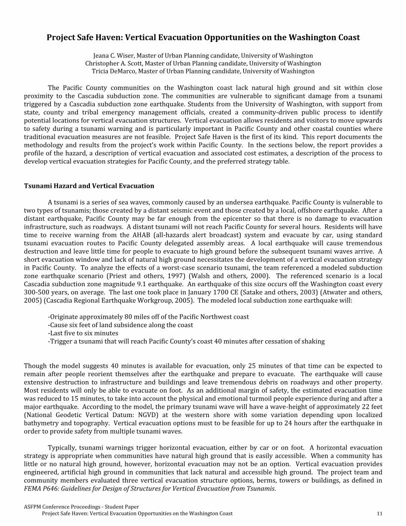
proximity to the Cascadia subduction zone. The communities are vulnerable to significant damage from a tsunami triggered by a Cascadia subduction zone earthquake. Students from the University of Washington, with support from state, county and tribal emergency management officials, created a community-driven public process to identify potential locations for vertical evacuation structures. Vertical evacuation allows residents and visitors to move upwards to safety during a tsunami warning and is particularly important in Pacific County and other coastal counties where traditional evacuation measures are not feasible. Project Safe Haven is the first of its kind. This report documents the methodology and results from the project’s work within Pacific County. In the sections below, the report provides a profile of the hazard, a description of vertical evacuation and associated cost estimates, a description of the process to develop vertical evacuation strategies for Pacific County, and the preferred strategy table.

Tsunami Hazard and Vertical Evacuation

A tsunami is a series of sea waves, commonly caused by an undersea earthquake. Pacific County is vulnerable to two types of tsunamis; those created by a distant seismic event and those created by a local, offshore earthquake. After a distant earthquake, Pacific County may be far enough from the epicenter so that there is no damage to evacuation infrastructure, such as roadways. A distant tsunami will not reach Pacific County for several hours. Residents will have time to receive warning from the AHAB (all-hazards alert broadcast) system and evacuate by car, using standard tsunami evacuation routes to Pacific County delegated assembly areas. A local earthquake will cause tremendous destruction and leave little time for people to evacuate to high ground before the subsequent tsunami waves arrive. A short evacuation window and lack of natural high ground necessitates the development of a vertical evacuation strategy in Pacific County. To analyze the effects of a worst-case scenario tsunami, the team referenced a modeled subduction zone earthquake scenario (Priest and others, 1997) (Walsh and others, 2000). The referenced scenario is a local Cascadia subduction zone magnitude 9.1 earthquake. An earthquake of this size occurs off the Washington coast every 300-500 years, on average. The last one took place in January 1700 CE (Satake and others, 2003) (Atwater and others, 2005) (Cascadia Regional Earthquake Workgroup, 2005). The modeled local subduction zone earthquake will:

-Originate approximately 80 miles off of the Pacific Northwest coast -Cause six feet of land subsidence along the coast -Last five to six minutes -Trigger a tsunami that will reach Pacific County’s coast 40 minutes after cessation of shaking Though the model suggests 40 minutes is available for evacuation, only 25 minutes of that time can be expected to remain after people reorient themselves after the earthquake and prepare to evacuate. The earthquake will cause extensive destruction to infrastructure and buildings and leave tremendous debris on roadways and other property. Most residents will only be able to evacuate on foot. As an additional margin of safety, the estimated evacuation time was reduced to 15 minutes, to take into account the physical and emotional turmoil people experience during and after a major earthquake. According to the model, the primary tsunami wave will have a wave-height of approximately 22 feet (National Geodetic Vertical Datum: NGVD) at the western shore with some variation depending upon localized bathymetry and topography. Vertical evacuation options must to be feasible for up to 24 hours after the earthquake in order to provide safety from multiple tsunami waves.

Typically, tsunami warnings trigger horizontal evacuation, either by car or on foot. A horizontal evacuation strategy is appropriate when communities have natural high ground that is easily accessible. When a community has little or no natural high ground, however, horizontal evacuation may not be an option. Vertical evacuation provides engineered, artificial high ground in communities that lack natural and accessible high ground. The project team and community members evaluated three vertical evacuation structure options, berms, towers or buildings, as defined in FEMA P646: Guidelines for Design of Structures for Vertical Evacuation from Tsunamis.

ASFPM Conference Proceedings - Student Paper Project Safe Haven: Vertical Evacuation Opportunities on the Washington Coast 12

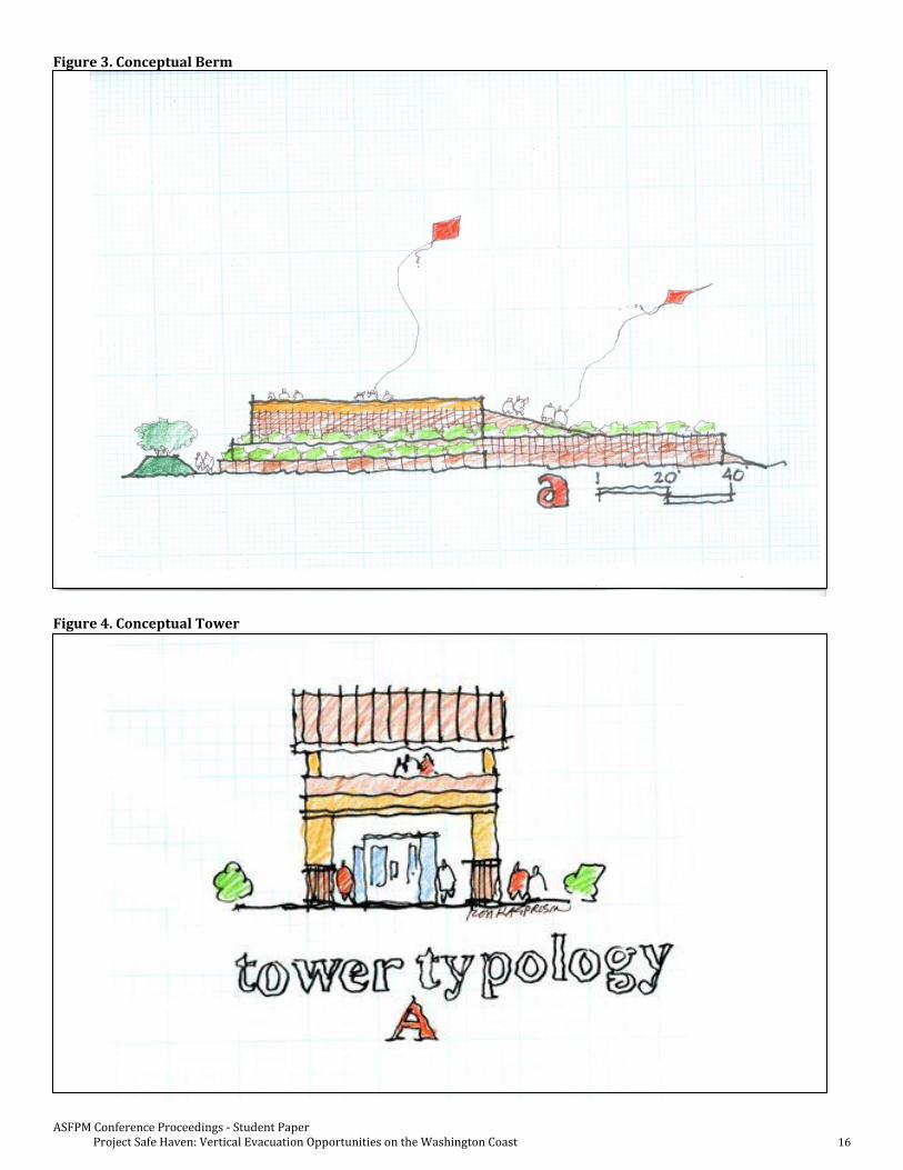
Berms are artificial high ground created from soil. They typically have ramps at a 1:4 slope providing access from the ground to the elevated surface. Berms have a large footprint on the landscape, giving the appearance of an engineered and designed hill. A berm has three component parts: a rounded front portion and gabion mound, the elevated safe haven area, and the access ramp. A berm can range in size from 1,000 square feet for 125 people up to 100,000 square feet for 12,500 people. The costs used for berm design were based primarily on RSMeans Unit Cost Data for 2010. According to this design, the cost of a berm increases equally with the addition of height or capacity. Estimated costs range from $300,000 – $900,000 depending on the required height and square footage.

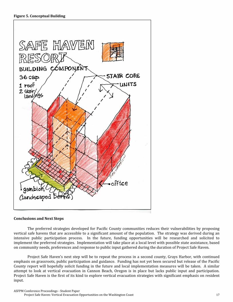
Towers can take the form of a simple elevated platform above the projected tsunami wave height, or a form such

as a lighthouse, that has a ramp or stairs leading to an elevation above projected wave height. A 500 square foot tower can hold 62 people and a 1,000 square foot tower can hold 125 people. The tower design used for construction cost estimates has five components: the foundation, a base isolation system, the support structure, superstructure, and methods of access. Two access options are included in the estimates; a breakaway stair system designed for daily use and for use to access the tower following a major earthquake. Following the tsunami event, evacuees would use a retractable staircase to leave the tower. The costs used for tower design were based primarily on RSMeans Building Construction Cost Data for 2010. Based on this generalized conceptual design, towers were determined to be the lowest cost. The cost of towers varies more greatly with increased capacity than with increased height. Estimated costs range from $110,000 - $170,000 depending on the required height and square footage.

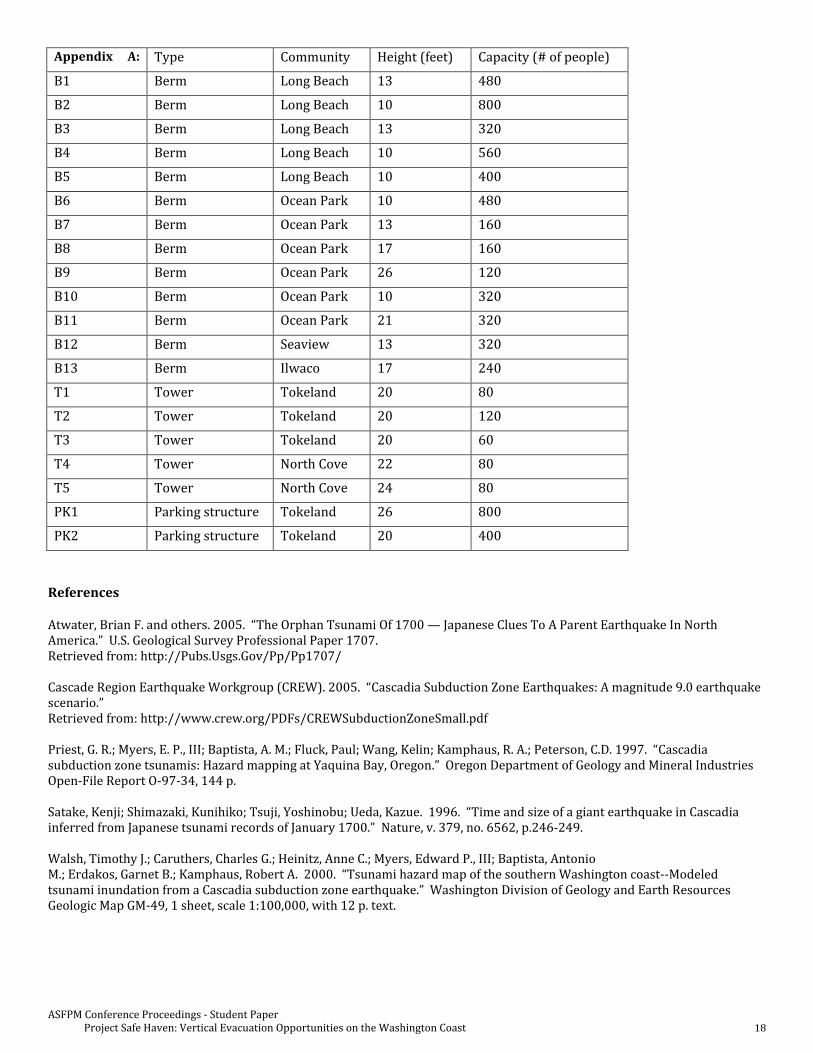
A building used as a tsunami evacuation structure has a ground floor that allows the tsunami wave to move

through it or is faced in a manner that the structural integrity of the building would support the force of the wave. Tsunami refugees seek safety in the upper floors of the building. Typical tsunami evacuation buildings are hotels or parking structures. For this project, the design used for construction cost estimates was based on citizen comments and preferences for two parking garages in the Tokeland area. In order to increase the likelihood of withstanding a tsunami, the first level of the building is considered “transparent,” having little surface area so as to reduce resistance against the force of the tsunami. The cost of a building depends greatly on the design requirements of the building’s primary use. The cost was based on parking garage cost according to the RSMeans Square Foot Costs Reference for 2010.

Methodology

In 2008, FEMA and NOAA released guidance on vertical evacuation. Several at-risk Pacific Coast communities began efforts to apply the FEMA guidance locally. In Pacific County, local officials documented their tsunami risk in the Pacific County Hazard Mitigation Plan. Under the direction of the state Earthquake and Tsunami Program Officer, Pacific County’s Emergency Manager, and the University of Washington Project Safe Haven, Pacific County was selected as the pilot community to conduct the first safe haven identification project. A steering committee composed of local and state officials, emergency managers, and scientists was established to guide the project and to select the targeted communities. Four Pacific County communities were selected as the project’s focus.

The team conducted site surveys in each of the four communities before initiating the public process. Unique

community attributes such as geography and land use were recognized and noted. Surveyed community attributes guided preparation for the first public meeting in each community and assisted with the development of approaches.

A series of two initial meetings were conducted in each community. The first meeting utilized the World Café

meeting process to identify and discuss the concept of vertical evacuation, various structure types, and conceptual site locations. The project team presented and discussed the alternatives that had been synthesized from the first meeting at the second meeting.

World Café meetings use “café style” conversations to facilitate small group brainstorming. During meeting #1

participants referenced large table maps of the community, in combination with walking circles and Lego models of vertical evacuation structures, to determine ideal placement locations. Each station represented a different type of vertical evacuation structure: berm, tower, or building. At the end of the World Café participants shared their discussion points and preferences for specific structure types and placement locations.

At meeting #2, the project team presented the alternatives derived from meeting #1 using maps and graphics.

Next, the team facilitated a large group brainstorming session regarding the strengths and weaknesses of each alternative using a strengths and weaknesses analysis technique. The goal of the meeting was to build consensus among those present and to develop a preferred strategy.

ASFPM Conference Proceedings - Student Paper Project Safe Haven: Vertical Evacuation Opportunities on the Washington Coast 13

After the series of initial community meetings were complete, the project team allowed time for the community

to mull and accept the preferred community strategies. The mulling process provided opportunities for both formal and informal community discussions about the preferred strategies. The project team occupied a booth at a Pacific County Emergency Preparedness Fair and presented preliminary strategies to the general public in the form of brochures and community profiles. The preliminary findings contributed to the community mulling process because it served as an educational component for residents who were unaware of Project Safe Haven. Ground-truth research at the site level for each proposed vertical evacuation site and solicitation of walking volunteers to confirm walking speed assumptions also took place during the community mulling process. Volunteers from all four communities participated in the walking study by walking from their home to the nearest proposed berm, tower, or buildings or assembly location and recording the time, distance, walking path, age, and any potential obstructions. This particular component of the project was essential in encouraging discussion, acceptance and excitement about the project. After the community was given time to mull, the project team reconvened to analyze data and develop the final strategy to be presented to the community. The team utilized new LiDAR elevation data in combination with wave height data for each conceptual site to determine necessary structure heights. Each conceptual site was designated berm, tower, parking structure, high ground, or assembly area. Some proposed berm sites were changed to high ground to reflect the new LiDAR elevation data.

The final conceptual sites were derived from the community participation processes with guidance from the

project team (Figures 1-2). The sites and strategies were confirmed during the community mulling process and ground-truthing trip. The maps were presented at the countywide meetings along with estimated capacities for each vertical evacuation site or structure (Appendix A). Two countywide meetings were held to confirm the preferred strategy and to receive further feedback about the project. Information about estimated costs, community processes, the tsunami hazard, and the intensive design workshops, commonly referred to as charrettes, was also presented.

ASFPM Conference Proceedings - Student Paper Project Safe Haven: Vertical Evacuation Opportunities on the Washington Coast 14

Figure 1. Preferred Vertical Evacuation Strategy: Long Beach Peninsula

ASFPM Conference Proceedings - Student Paper Project Safe Haven: Vertical Evacuation Opportunities on the Washington Coast 15

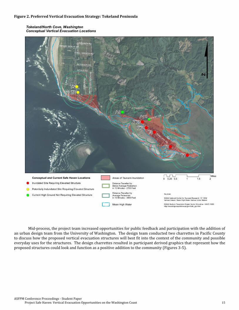
Figure 2. Preferred Vertical Evacuation Strategy: Tokeland Peninsula

Mid-process, the project team increased opportunities for public feedback and participation with the addition of an urban design team from the University of Washington. The design team conducted two charrettes in Pacific County to discuss how the proposed vertical evacuation structures will best fit into the context of the community and possible everyday uses for the structures. The design charrettes resulted in participant derived graphics that represent how the proposed structures could look and function as a positive addition to the community (Figures 3-5).

ASFPM Conference Proceedings - Student Paper Project Safe Haven: Vertical Evacuation Opportunities on the Washington Coast 16

Figure 3. Conceptual Berm

Figure 4. Conceptual Tower

ASFPM Conference Proceedings - Student Paper Project Safe Haven: Vertical Evacuation Opportunities on the Washington Coast 17

Figure 5. Conceptual Building

Conclusions and Next Steps

The preferred strategies developed for Pacific County communities reduces their vulnerabilities by proposing

vertical safe havens that are accessible to a significant amount of the population. The strategy was derived during an intensive public participation process. In the future, funding opportunities will be researched and solicited to implement the preferred strategies. Implementation will take place at a local level with possible state assistance, based on community needs, preferences and response to public input gathered during the duration of Project Safe Haven.

Project Safe Haven’s next step will be to repeat the process in a second county, Grays Harbor, with continued

emphasis on grassroots, public participation and guidance. Funding has not yet been secured but release of the Pacific County report will hopefully solicit funding in the future and local implementation measures will be taken. A similar attempt to look at vertical evacuation in Cannon Beach, Oregon is in place but lacks public input and participation. Project Safe Haven is the first of its kind to explore vertical evacuation strategies with significant emphasis on resident input.

ASFPM Conference Proceedings - Student Paper Project Safe Haven: Vertical Evacuation Opportunities on the Washington Coast 18

Appendix A:

Pacific

County

Preferred

Vertical

Evacuation

Strategy

TableMap

Legend

Type Community Height (feet) Capacity (# of people)

B1 Berm Long Beach 13 480

B2 Berm Long Beach 10 800

B3 Berm Long Beach 13 320

B4 Berm Long Beach 10 560

B5 Berm Long Beach 10 400

B6 Berm Ocean Park 10 480

B7 Berm Ocean Park 13 160

B8 Berm Ocean Park 17 160

B9 Berm Ocean Park 26 120

B10 Berm Ocean Park 10 320

B11 Berm Ocean Park 21 320

B12 Berm Seaview 13 320

B13 Berm Ilwaco 17 240

T1 Tower Tokeland 20 80

T2 Tower Tokeland 20 120

T3 Tower Tokeland 20 60

T4 Tower North Cove 22 80

T5 Tower North Cove 24 80

PK1 Parking structure Tokeland 26 800

PK2 Parking structure Tokeland 20 400

References

Atwater, Brian F. and others. 2005. “The Orphan Tsunami Of 1700 — Japanese Clues To A Parent Earthquake In North America.” U.S. Geological Survey Professional Paper 1707. Retrieved from: http://Pubs.Usgs.Gov/Pp/Pp1707/

Cascade Region Earthquake Workgroup (CREW). 2005. “Cascadia Subduction Zone Earthquakes: A magnitude 9.0 earthquake scenario.” Retrieved from: http://www.crew.org/PDFs/CREWSubductionZoneSmall.pdf

Priest, G. R.; Myers, E. P., III; Baptista, A. M.; Fluck, Paul; Wang, Kelin; Kamphaus, R. A.; Peterson, C.D. 1997. “Cascadia subduction zone tsunamis: Hazard mapping at Yaquina Bay, Oregon.” Oregon Department of Geology and Mineral Industries Open-File Report O-97-34, 144 p. Satake, Kenji; Shimazaki, Kunihiko; Tsuji, Yoshinobu; Ueda, Kazue. 1996. “Time and size of a giant earthquake in Cascadia inferred from Japanese tsunami records of January 1700.” Nature, v. 379, no. 6562, p.246-249. Walsh, Timothy J.; Caruthers, Charles G.; Heinitz, Anne C.; Myers, Edward P., III; Baptista, Antonio M.; Erdakos, Garnet B.; Kamphaus, Robert A. 2000. “Tsunami hazard map of the southern Washington coast--Modeled tsunami inundation from a Cascadia subduction zone earthquake.” Washington Division of Geology and Earth Resources Geologic Map GM-49, 1 sheet, scale 1:100,000, with 12 p. text.

ASFPM Conference Proceedings - Student Paper The Effect of Land-Cover Changes on Lag Time in the Banklick Creek Watershed, KY 19

The Effect of Land-cover Changes on Lag Time in the Banklick Creek Watershed, KY

Katelyn Toebbe, University of Louisville Department of Geography and Geosciences

Introduction

Urbanization in a watershed is known to affect the entire balance of the water network, often resulting in more frequent and severe flooding. In a natural environment, precipitation is: intercepted by vegetation and evapotranspired back into the atmosphere, stored in the soil, transported as overland flow to low order streams, or percolated down to the water table (Yang et al., 2009). The prevalence of impervious surfaces in urban areas retards penetration and infiltration and reduces friction and meandering, drastically increasing flow velocity and erosive force. The result is an increased amount of runoff, moving faster, meaning a shorter lag time to discharge. This manifests itself in less groundwater recharge and higher flood peaks (Wheater and Evans, 2009). Another result of urban development is the destruction of first and second order streams, which also contributes to flooding (Brilly et al. 2006).

The effects of urbanization on flooding have been widely investigated in the scientific community because in an urban environment, flooding is a threat to citizens and infrastructure (Yang et al. 2010). In a 2010 study, a team from Purdue University led by Gouxian Yang investigated the response of watersheds to urbanization in the White River Basin, Indiana. They made land use classes using unsupervised classification of Landsat thematic mapper (TM) and used them in an altered Anderson level- 2 classification scheme. They estimated high density urban pixels as 90 percent impervious area, and 35 percent low density. These are according to the Environmental Protection Agency (EPA)'s definition, that 80-100% of highly urbanized areas are impervious, and 20-49% of low-density urbanization is impervious (Yang et al. 2010). This helps account for the error introduced from a large pixel size, which may capture mixed land-cover types.

Methodology

a.) Study Area

The Banklick Creek watershed is a 58-square mile basin covering much of Kenton County and a small portion of Boone County, Kentucky. The creek itself is 19.2 miles long and drains northeast into the Licking River. It has six main tributaries including: Brushy Fork, Bullock Pen Creek, Fowler Creek, Holds Branch, Horse Branch, and Wolf Pen Branch. An active USGS gauging station, number 03254550, is present on the stream in the city of Erlanger, capturing 58% of the drainage area (Limnotech 2009). The topography surrounding Banklick is mostly rolling hills, many with steep slopes. It is underlain by limestone and shale. A majority of the soils in the area are considered hydrologic soil group “C”, and are easily eroded and are not conducive to infiltration when wet (Limnotech, 2009). The climate is temperate, characterized by humid, hot summers and relatively cold winters. The range of temperature averages annually is from 33°F to 76°F, and precipitation averages 42 inches (USDA Forest Service, 2007).

This watershed has been developing drastically in the past twenty years, although in the last ten, this development has been predominately in the headwaters and on ridges and slopes, which certainly has an impact on the watershed dynamics. This development along with the steep slopes of the Banklick channel and its tributaries, and the dense development along the stream channel early on, were identified as the three major causes of flooding in this creek by the US Army Corp of Engineers (Limnotech, 2009). The USGS gauging station used captures the area of interest for this study, the headwaters in the southern portion of the basin. The land cover classification was run for the entire watershed to better understand the overall basin characteristics; not much change is seen in the densely developed northern portion.

b.) Data

Discharge data from USGS station # 03254550 dates back to 1999, and was obtained in fifteen- minute increments for a ten-year study period from 2000 to 2010. Precipitation data was received from the National Climatic Data Center (NCDC) for station number 151855, the Covington, KY station at the Greater Cincinnati Airport, located approximately 3.5 miles from the Banklick Creek basin. The precipitation data from 2000 til May of 2010 was

ASFPM Conference Proceedings - Student Paper The Effect of Land-Cover Changes on Lag Time in the Banklick Creek Watershed, KY 20

obtained. Since there was not a full year's record for 2010, the decision was made to narrow the study period into four year increments, with study years of 2001, 2005, and 2009 to capture the trend of the 2000 decade. The three largest discharge events in each study year were identified and averaged into hourly records so that the two data types were in equal units. To quantify the urban growth in the Banklick Creek watershed over the last ten years, Landsat 4-5 Thematic Mapper (TM) images were obtained from 2000 to 2010 and classified. All images were taken in August and September. This ensures consistency of season, but also allows for enough selection for high-quality images (ranked 9 by NASA) with low (less than 30 %) cloud cover. The images were ordered using the United States Geological Survey (USGS) Global Visualizer (GloVis). Landsat bands 1 through 5 were stacked in ENVI+IDL by date and loaded into an RGB display using bands 4, 3, 2, creating a false-color image. The displays were then enhanced by using a Gaussian stretch tool to apply a normal distribution to the pixel values. This minimizes the possibility of variation between the images due to variations in the image capture, such as time of day, etc.

An unsupervised iterative self-organizing data analysis (ISODATA) classification was run to gain basic knowledge of the land cover classes in the study area. A maximum likelihood supervised classification was then performed in ENVI 4.8 to create major land cover classes in the area. Six classes were used, including forest, agriculture/grass, highly impervious, partial impervious, water, and bare ground. The forest class captures bushy dense vegetation and the agriculture class includes not only cropland but all low-lying less dense vegetation, such as lawns. Highly impervious areas are areas of definite impermeability, such as warehouses, city centers, and airports. The “partial impervious” class includes areas of mixed pixel values characteristic of suburban development, a mix of impermeability and grass. The water class was needed to capture water bodies in the area. “Bare Ground” is a necessary class due to its unique reflectance; it is important to define it separately from impervious surfaces. Pixel values between years may fluctuate between agriculture and bare ground due to weather conditions.

Change detection was then run in four-year increments, 2001-2005, and 2005 to 2010. Unfortunately, every Landsat image taken of the study area for the summer months in 2009 has detrimental cloud cover, making accurate analysis difficult. The decision was made to use 2010 imagery instead. This allows for capture of the land-cover change, although impervious surface values may be slightly over-estimated because of this.

Next, a watershed boundary shapefile was imported into ENVI 4.8 to limit analysis to the study area alone. Change detection statistics in ENVI 4.8 were then run to provide a detailed summary of the changes of land cover classes between each set of images, showing the changes from each class to another. In accordance with EPA guidelines, anything classified as “highly impervious” in this study is considered 95% impervious cover and “partially impervious” is considered 40% impervious.

Results

Table 1 shows the three top discharge events for the study years of 2001, 2005, and 2009. They are sorted by year and discharge in cubic feet per second (cfs). The date and military time are listed for both the precipitation and discharge peaks. The calculated lag times between precipitation peaks and discharge responses are shown, which are the focus of the study.

Table 1. Precipitation, Discharge, and Lag Time, Top 3 discharge events for 2001, 2005, and 2009

Peak Precipitation Peak Discharge Lag Time

1-3870 cfs 10/24/01 3:00 10/24/01 7:00 4 hrs

2001 Events 0-2650 cfs 7/18/01 0:00 7/18/01 4:00 4 hrs

2-2100 cfs 6/6/01 15:00 6/6/01 18:00 3 hrs

#1- 5360 cfs 3/28/05 3:00 3/28/05 4:00 1 hr

2005 Events #2- 5010 cfs 11/15/05 4:00 11/15/05 7:00 3 hrs

#3- 3830 cfs 1/3/05 9:00 1/3/05 11:00 2 hrs

#1- 9490 cfs 7/30/09 22:00 7/31/09 2:00 4 hrs

2009 Events #2- 1860 cfs 10/9/09 0:00 10/9/09 6:00 6 hrs

#3- 1810 cfs 2/27/09 3:00 2/27/09 7:00 4 hrs

ASFPM Conference Proceedings - Student Paper The Effect of Land-Cover Changes on Lag Time in the Banklick Creek Watershed, KY 21

Figures one through three show the Landsat images for 2001, 2005, and 2010 respectively, that were

classified and clipped to the Banklick Creek watershed. The class in red is highly impervious, magenta is partially impervious, green is dense vegetation such as forests, yellow is low-lying vegetation capturing grass and agriculture, and sienna is bare ground. Image Classification Results:

Figure 1. August 2001 Classified Image Figure 2. August 2005 Classified Image Figure 3. September 2010 Classified Image

Lag time was measured as clearly increasing between 2001 and 2005 (Table 1), which shows the effect of urban

development in the headwaters seen in the Figure 3, and not Figure 2. There is a 13,664,745 m2 increase in impervious surface area measured in this time. This area is calculated by multiplying the highly impervious surface area by 95% and adding it with 40% of the partially impervious area in Table 2. The increases in impervious land cover types are accompanied by a decrease in forest and agriculture or bare ground, which further confirms the development trends.

In 2005, many neighborhoods were under construction. These areas of packed ground and gravel were classified as highly impervious (red). Much of these clusters are then classified as partially impervious in the 2010 image (Figure 3). After construction, these sites were regraded and seeded, and lawns and vegetation were established.

This is why even though there is still an increase in impervious surface area from 2005 to 2010 of 5,538,240 m2, lag time is seen to go back up. The results suggest that even though there is significant development between 2001 and 2009, since the land has had time to allow growth of vegetation, the water is slowed back down to a longer lag time between precipitation peaks and discharge peaks. The 2005 image had a much larger “bare ground” class due to a drought that year, with the area only receiving 38.8 inches of precipitation. This creates a false increase in agriculture between 2005 and 2010 with the decrease in bare ground as the vegetation in these areas was reinstated.

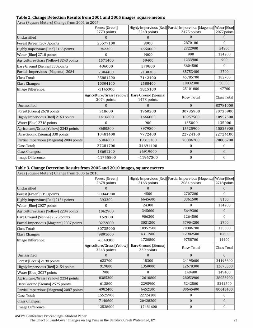
ASFPM Conference Proceedings - Student Paper The Effect of Land-Cover Changes on Lag Time in the Banklick Creek Watershed, KY 22

Table 2. Change Detection Results from 2001 and 2005 images, square meters Area (Square Meters) Change from 2001 to 2005

Forest [Green] 2779 points

Highly Impervious [Red] 2248 points

Partial Impervious [Magenta] 2475 points

Water [Blue] 2077 points

Unclassified 0 0 0 0

Forest [Green] 2678 points 25577100 9900 2870100 0

Highly Impervious [Red] 2163 points 942300 4554000 2322900 54900

Water [Blue] 2718 points 0 9000 900 124200

Agriculture/Grass [Yellow] 3243 points 1571400 59400 1233900 900

Bare Ground [Sienna] 330 points 486000 379800 3604500 0

Partial Impervious [Magenta] 2084 points

7304400 2130300 35753400 2700

Class Total; 35881200 7142400 45785700 182700

Class Changes: 10304100 2588400 10032300 58500

Image Difference: -5145300 3815100 25101000 -47700

Agriculture/Grass [Yellow]

2074 points Bare Ground [Sienna]

1473 points Row Total Class Total

Unclassified 0 0 0 83781000

Forest [Green] 2678 points 318600 1960200 30735900 30735900

Highly Impervious [Red] 2163 points 1416600 1666800 10957500 10957500

Water [Blue] 2718 points 0 900 135000 135000

Agriculture/Grass [Yellow] 3243 points 8680500 3979800 15525900 15525900

Bare Ground [Sienna] 330 points 10481400 7772400 22724100 22724100

Partial Impervious [Magenta] 2084 points 6384600 19311300 70886700 70886700

Class Total; 27281700 34691400 0 0

Class Changes: 18601200 26919000 0 0

Image Difference: -11755800 -11967300 0 0

Table 3. Change Detection Results from 2005 and 2010 images, square meters

Area (Square Meters) Change from 2005 to 2010

Forest [Green] 2678 points

Highly Impervious [Red] 2163 points

Partial Impervious [Magenta] 2084 points

Water [Blue] 2718 points

Unclassified 0 0 0 0

Forest [Green] 2198 points 20844900 4500 2707200 0

Highly Impervious [Red] 2154 points 393300 6645600 3361500 8100

Water [Blue] 2027 points 0 24300 0 124200

Agriculture/Grass [Yellow] 2234 points 1062900 345600 5649300 0

Bare Ground [Sienna] 2575 points 162000 906300 1264500 0

Partial Impervious [Magenta] 2087 points 8272800 3031200 57904200 2700

Class Total; 30735900 10957500 70886700 135000

Class Changes: 9891000 4311900 12982500 10800

Image Difference: -6540300 1720800 9758700 14400

Agriculture/Grass [Yellow]

3243 points Bare Ground [Sienna]

330 points Row Total Class Total

Unclassified 0 0 0 0

Forest [Green] 2198 points 623700 15300 24195600 24195600

Highly Impervious [Red] 2154 points 919800 1350000 12678300 12678300

Water [Blue] 2027 points 900 0 149400 149400

Agriculture/Grass [Yellow] 2234 points 8385300 12610800 28053900 28053900

Bare Ground [Sienna] 2575 points 613800 2295900 5242500 5242500

Partial Impervious [Magenta] 2087 points 4982400 6452100 80645400 80645400

Class Total; 15525900 22724100 0 0

Class Changes: 7140600 20428200 0 0

Image Difference: 12528000 -17481600 0 0

ASFPM Conference Proceedings - Student Paper The Effect of Land-Cover Changes on Lag Time in the Banklick Creek Watershed, KY 23

Conclusions The results of this study clearly show the effect that land cover has on lag time between precipitation and discharge peaks. Urbanization reduces infiltration and speeds up runoff, effectively reducing lag time, increasing the frequency and magnitude of flooding. The later results, however, show how with some time for vegetation to develop, lag time can be brought back up. It is critical that policy makers consider these effects when making zoning laws and considering flood mitigation. An effort should be made to preserve low-order streams and restore natural vegetation to prevent further flooding in a stream. Further studies beneficial to the understanding of this watershed could include higher resolution data, both in imagery and shorter-increment precipitation and discharge data. A larger, longer term study would be beneficial to have enough data to run significance tests. Hydrologic modeling such as HEC-HMS or the EPA's SWMM model could also be used to project future and model past conditions.

References

Brilly, M., Rusjan, S. and A. Vidmar. 2006. Monitoring the Impact of Urbanisation on the Glinscica Stream. Physics and Chemistry of the Earth 31: 1089-1096

Limnotech. 2009. Banklick Creek Watershed Characterization Report. Prepared for Sanitation District No. 1 of Northern Kentucky USDA Forest Service. 2007. Conditions & Closures: Climate in Kentucky. Available at: http://www.fs.fed.us/r8/boone/conditions/clim.shtml (last accessed 14 March 2010).

Wheater, H. and E. Evans. 2009. Land use, water management and future flood risk. Land Use Policy 26 (1): S25 1-S264

Yang, G., Bowling, L.C., Cherkauer, K. A., Pijanowski, B.C., and D. Niyogi. 2009. Hydro climatic Response of Watersheds to Urban Intensity: An Observational and Modeling-Based Analysis for the White River Basin, Indiana. Journal of Hydrometeorology 11: 122-138

ASFPM Conference Proceedings - Student Paper Uncertainty Analysis in Flood Inundation Mapping 24

Uncertainty Analysis in Flood Inundation Mapping

Younghun Jung and Venkatesh Merwade Purdue University

Abstract

The accuracy of flood inundation maps is determined by the uncertainty propagated from all variables involved in

the overall process including input data, model parameters and modeling approaches. This study investigates the

uncertainty arising from key variables (discharge, topography, and Manning’s n) among model variables in the East Fork

White River near Seymour, Indiana. Methodology of this study involves the first order approximation (FOA) method to

estimate the propagated uncertainty rates and the generalized likelihood uncertainty estimation (GLUE) to quantify the

uncertainty bounds. Uncertainty bounds in the GLUE procedure are evaluated by selecting a likelihood function, which is

a statistic (F-statistic) based on the area of observed and simulated flood inundation map. The results from GLUE show

that the uncertainty propagated from multiple variables produce an uncertainty bound of about 15% in the inundation

area compared to observed inundation.

Introduction and Objectives

Quantifying the role of uncertainty is critical for the improvement of flood prediction capabilities. Uncertainty in

flood inundation mapping arises from input data as well as modeling approaches including hydraulic modeling,

hydrologic modeling, and terrain analysis. Although the variables contributing to uncertainties in flood inundation

mapping are well documented by several studies (Romanowicz and Beven 1998; Pappenberger et al. 2005, 2006;

Merwade et al., 2008), it is impossible to completely remove these uncertainties due to constraints imposed by time,

cost, technology, and knowledge. Similarly, although the uncertain variables in flood inundation mapping are known, not

all of them contribute equally to the final uncertainty in the flood inundation map for a given circumstance. Therefore,

deciding the priority among the elements that cause uncertainty is the first step, and reducing the sources of uncertainty

for the prioritized variables is the second step in reducing the overall uncertainty in flood inundation mapping.

The objectives of this study are to: (i) estimate the propagated uncertainty rates of key variables in flood inundation

mapping by using the first order approximation (FOA) method; and (ii) quantify the uncertainty bounds arising from

multiple variables using the generalized likelihood uncertainty estimate (GLUE). Monte Carlo (MC) simulations using

HEC-RAS and triangle based interpolation are performed to investigate the uncertainty arising from discharge,

topography, and Manning’s n in East Fork White River near Seymour, Indiana as a study site.

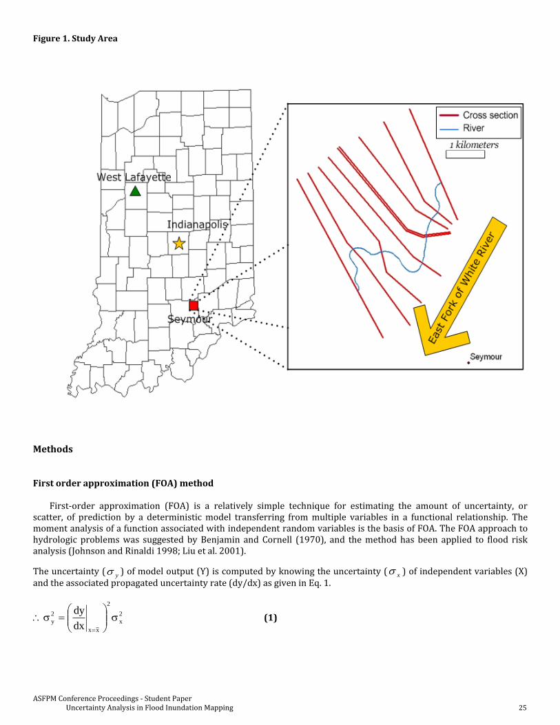
Study Area and Data

This study is performed along a 5 km reach (Seymour reach) of the East Fork of the White River near Seymour

Indiana (Figure 1). The East Fork of the White River begins in Columbus, Indiana, and joins the West Fork of the White

River before draining into the Wabash River. The region around the selected Seymour reach was affected by the July

2008 flood event. The Seymour reach is characterized by a relatively wide floodplain with U shaped cross-sections. The

topography data for extracting cross-sections and flood inundation mapping is obtained from the digital elevation model

(DEM) from the 2005 IndianaMap Color Orthophotography Project by Indiana University. A total of nine cross-sections

are extracted from the 1.5m horizontal resolution DEM. The average width of the Seymour reach cross-sections is 3.9km

with an average spacing of 700m. The flow data used for hydraulic modeling of the Seymour reach include the observed

discharge of 2729.7m3/s with a reach boundary condition of downstream normal depth. The land use for the Seymour

reach main channel ranges from a Manning’s n value of 0.04 to 0.05. In the floodplains, the Manning’s n value ranges

from a value of 0.04 to 0.12.

ASFPM Conference Proceedings - Student Paper Uncertainty Analysis in Flood Inundation Mapping 25

Figure 1. Study Area

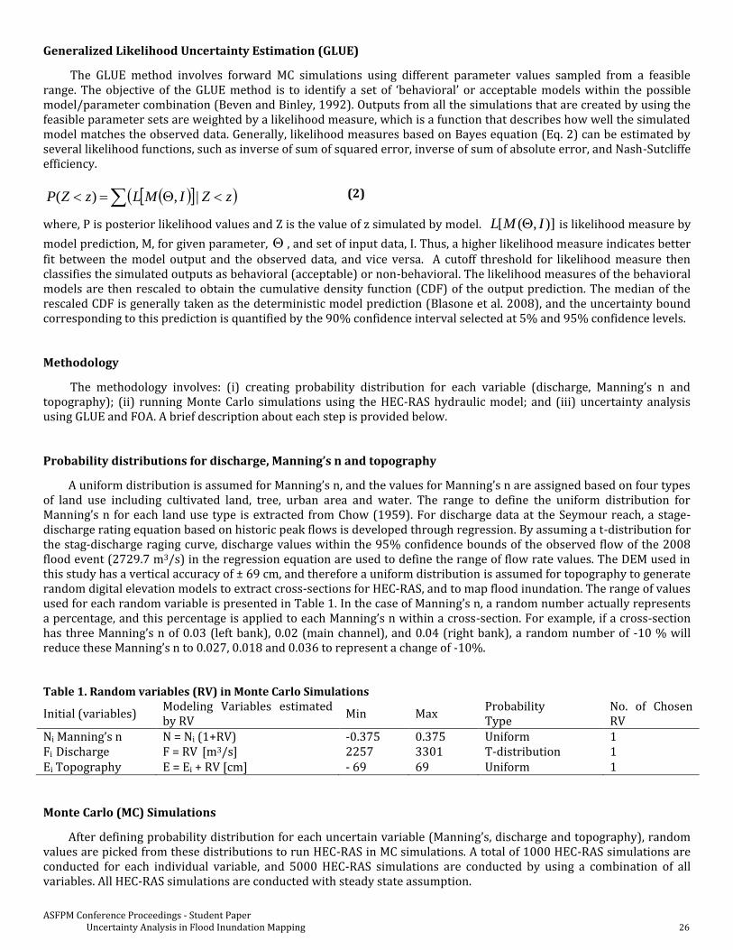
Methods First order approximation (FOA) method

First-order approximation (FOA) is a relatively simple technique for estimating the amount of uncertainty, or scatter, of prediction by a deterministic model transferring from multiple variables in a functional relationship. The moment analysis of a function associated with independent random variables is the basis of FOA. The FOA approach to hydrologic problems was suggested by Benjamin and Cornell (1970), and the method has been applied to flood risk analysis (Johnson and Rinaldi 1998; Liu et al. 2001). The uncertainty (

y ) of model output (Y) is computed by knowing the uncertainty ( x ) of independent variables (X) and the associated propagated uncertainty rate (dy/dx) as given in Eq. 1.

2

x

2

xx

2

ydx

dy

(1)

ASFPM Conference Proceedings - Student Paper Uncertainty Analysis in Flood Inundation Mapping 26

Generalized Likelihood Uncertainty Estimation (GLUE)

The GLUE method involves forward MC simulations using different parameter values sampled from a feasible range. The objective of the GLUE method is to identify a set of ‘behavioral’ or acceptable models within the possible model/parameter combination (Beven and Binley, 1992). Outputs from all the simulations that are created by using the feasible parameter sets are weighted by a likelihood measure, which is a function that describes how well the simulated model matches the observed data. Generally, likelihood measures based on Bayes equation (Eq. 2) can be estimated by several likelihood functions, such as inverse of sum of squared error, inverse of sum of absolute error, and Nash-Sutcliffe efficiency.

(2)

where, P is posterior likelihood values and Z is the value of z simulated by model. )],([ IML is likelihood measure by

model prediction, M, for given parameter, , and set of input data, I. Thus, a higher likelihood measure indicates better fit between the model output and the observed data, and vice versa. A cutoff threshold for likelihood measure then classifies the simulated outputs as behavioral (acceptable) or non-behavioral. The likelihood measures of the behavioral models are then rescaled to obtain the cumulative density function (CDF) of the output prediction. The median of the rescaled CDF is generally taken as the deterministic model prediction (Blasone et al. 2008), and the uncertainty bound corresponding to this prediction is quantified by the 90% confidence interval selected at 5% and 95% confidence levels. Methodology

The methodology involves: (i) creating probability distribution for each variable (discharge, Manning’s n and topography); (ii) running Monte Carlo simulations using the HEC-RAS hydraulic model; and (iii) uncertainty analysis using GLUE and FOA. A brief description about each step is provided below.

Probability distributions for discharge, Manning’s n and topography

A uniform distribution is assumed for Manning’s n, and the values for Manning’s n are assigned based on four types of land use including cultivated land, tree, urban area and water. The range to define the uniform distribution for Manning’s n for each land use type is extracted from Chow (1959). For discharge data at the Seymour reach, a stage-discharge rating equation based on historic peak flows is developed through regression. By assuming a t-distribution for the stag-discharge raging curve, discharge values within the 95% confidence bounds of the observed flow of the 2008 flood event (2729.7 m3/s) in the regression equation are used to define the range of flow rate values. The DEM used in this study has a vertical accuracy of ± 69 cm, and therefore a uniform distribution is assumed for topography to generate random digital elevation models to extract cross-sections for HEC-RAS, and to map flood inundation. The range of values used for each random variable is presented in Table 1. In the case of Manning’s n, a random number actually represents a percentage, and this percentage is applied to each Manning’s n within a cross-section. For example, if a cross-section has three Manning’s n of 0.03 (left bank), 0.02 (main channel), and 0.04 (right bank), a random number of -10 % will reduce these Manning’s n to 0.027, 0.018 and 0.036 to represent a change of -10%.

Table 1. Random variables (RV) in Monte Carlo Simulations

Initial (variables) Modeling Variables estimated by RV

Min Max Probability Type

No. of Chosen RV

Ni Manning’s n N = Ni (1+RV) -0.375 0.375 Uniform 1 Fi Discharge F = RV [m3/s] 2257 3301 T-distribution 1 Ei Topography E = Ei + RV [cm] - 69 69 Uniform 1

Monte Carlo (MC) Simulations

After defining probability distribution for each uncertain variable (Manning’s, discharge and topography), random values are picked from these distributions to run HEC-RAS in MC simulations. A total of 1000 HEC-RAS simulations are conducted for each individual variable, and 5000 HEC-RAS simulations are conducted by using a combination of all variables. All HEC-RAS simulations are conducted with steady state assumption.

zZIMLzZP |,)(

ASFPM Conference Proceedings - Student Paper Uncertainty Analysis in Flood Inundation Mapping 27

Estimation of the propagated uncertainty rate using the FOA method

FOA method requires a mathematical equation that relates random variables with model output to define the rate of propagation uncertainty in Eq. 1. In this study, a regression equation is developed to define a mathematical relationship between each target random variable (Manning’s n, discharge and topography) and flood inundation area. The propagated uncertainty rate is estimated through 1000 MC simulations for each variable. The propagated uncertainty rate is computed by taking the ratio of flood inundation area to the change rate (%) of each target random variable. This ratio defines the dy/dx term in Eq.1.

Quantification of uncertainty using GLUE

After MC simulations, all outputs are evaluated by a likelihood measure to reflect how well the simulated model compares with the observed or baseline output. The selection of a likelihood measure is a subjective process, and the uncertainty bound obtained using GLUE is affected by the choice of the likelihood measure. In this study, F-statistic (Eq. 3) that includes the spatial aspects of a flood inundation map is used to estimate the likelihood measure for the uncertainty bound.

(3)

where Ao indicates the observed inundation area, Ap refers to the predicted flood inundation area, and Aop represents the intersection of both observed and predicted inundation areas. Uncertainty bound using GLUE is estimated based on the output of MC simulations. Table 2. MC simulation results for Seymour Reach (Area in Km2)

Combination Manning’s n Topography Discharge

Min 6.706 9.935 9.204 10.441

Max 11.085 10.814 10.957 10.675

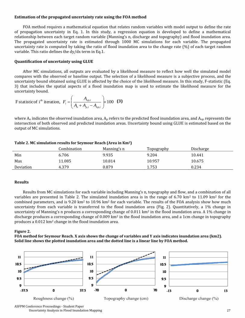
Deviation 4.379 0.879 1.753 0.234 Results

Results from MC simulations for each variable including Manning’s n, topography and flow, and a combination of all variables are presented in Table 2. The simulated inundation area is in the range of 6.70 km2 to 11.09 km2 for the combined parameters, and is 9.20 km2 to 10.96 km2 for each variable. The results of the FOA analysis show how much uncertainty from each variable is transferred to the flood inundation area (Fig. 2). Quantitatively, a 1% change in uncertainty of Manning’s n produces a corresponding change of 0.011 km2 in the flood inundation area. A 1% change in discharge produces a corresponding change of 0.009 km2 in the flood inundation area, and a 1cm change in topography produces a 0.012 km2 change in the flood inundation area. Figure 2. FOA method for Seymour Reach. X axis shows the change of variables and Y axis indicates inundation area (km2). Solid line shows the plotted inundation area and the dotted line is a linear line by FOA method.

100,iteration i of statistic F,,

,th

iopipo

iop

iAAA

AF

ASFPM Conference Proceedings - Student Paper Uncertainty Analysis in Flood Inundation Mapping 28

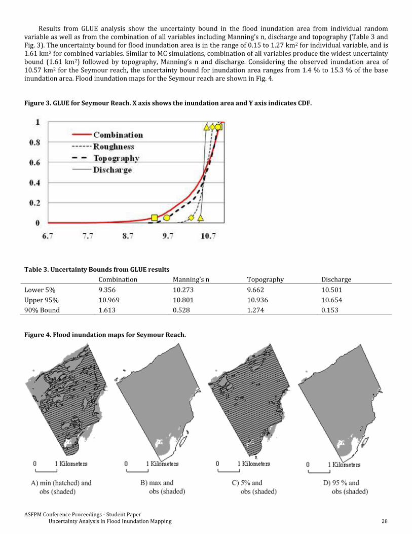
Results from GLUE analysis show the uncertainty bound in the flood inundation area from individual random variable as well as from the combination of all variables including Manning’s n, discharge and topography (Table 3 and Fig. 3). The uncertainty bound for flood inundation area is in the range of 0.15 to 1.27 km2 for individual variable, and is 1.61 km2 for combined variables. Similar to MC simulations, combination of all variables produce the widest uncertainty bound (1.61 km2) followed by topography, Manning’s n and discharge. Considering the observed inundation area of 10.57 km2 for the Seymour reach, the uncertainty bound for inundation area ranges from 1.4 % to 15.3 % of the base inundation area. Flood inundation maps for the Seymour reach are shown in Fig. 4.

Figure 3. GLUE for Seymour Reach. X axis shows the inundation area and Y axis indicates CDF.

Table 3. Uncertainty Bounds from GLUE results

Combination Manning’s n Topography Discharge

Lower 5% 9.356 10.273 9.662 10.501

Upper 95% 10.969 10.801 10.936 10.654

90% Bound 1.613 0.528 1.274 0.153 Figure 4. Flood inundation maps for Seymour Reach.

ASFPM Conference Proceedings - Student Paper Uncertainty Analysis in Flood Inundation Mapping 29

Conclusions The following conclusions are drawn from this study: This study presents an approach for quantifying the uncertainty and the propagation of uncertainty in flood

inundation mapping using FOA and GLUE methods. FOA analysis using the 2008 flood data on the Seymour reach shows that the propagation of uncertainty is highest for topography followed by Manning’s n and discharge.

The GLUE analysis also showed that topography emerged as the top uncertain variable for the Seymour Reach. This finding can be attributed to the accuracy of topography data in flood inundation modeling and mapping. This conclusion is consistent with past studies that have found the accuracy of topography data to play a major role in flood inundation mapping.

The uncertainty bound from each variable does not add up to produce the combined uncertainty bound, thus demonstrating the non-linear nature of uncertainty propagation in the overall flood inundation mapping process.

The findings of this study are based on one single reach in Indiana. More studies using different topographic and flow conditions are needed to generalize the role of uncertainty and uncertainty propagation in flood inundation mapping.

References Benjamin, J.R. and Cornell, C.A. 1970 “Probability, Statistics and Decision Making for Civil Engineers.” McGraw-Hill, New York, N.Y. Beven, K. J., and Binley, A. M. 1992 “The future of distributed models: model calibration and uncertainty prediction.” Hydrol. Process, 279-298. Blasone, R.-S., J. A. Vrugt, H. Madsen, D. Rosbjerg, B. A. Robinson, and G. A. Zyvoloski 2008 “Generalized likelihood uncertainty estimation (GLUE) using adaptive Markov chain Monte Carlo sampling.” Adv. Water Resour., 31, 630–648. Chow, V.T. 1959 “Open-channel hydraulics.” New York, McGraw-Hill Johnson, P. A., and Rinaldi, M. 1998 “Uncertainty in stream channel restoration. Uncertainty modeling and analysis in civil engineering.” B. M. Ayyub, ed., CRC Press, Boca Raton, Fla., 425–437. Liu, J., Tian, F., and Huang, Q. 2001 “A risk analyzing method for reservoir flood control.” Hydrology, 21(3): 1-3. Merwade, V.M., Olivera, F., Arabi, M., and Edleman, S. 2008 “Uncertainty in flood inundation mapping – current issues and future directions.” ASCE Journal of Hydrologic Engineering, 13 (7), 608–620 Pappenberger, F., K. Beven, et al. 2005 “Uncertainty in the calibration of effective roughness parameters in HEC-RAS using inundation and downstream level observations.” Journal of Hydrology 302(1-4): 46-69 Pappenberger, F., P. Matgen, et al. 2006 “Influence of uncertain boundary conditions and model structure on flood inundation predictions.” Advances in Water Resources 29(10): 1430-1449 Romanowicz, R. and Beven, K.J. 1998 “Dynamic real-time prediction of flood inundation probabilities.” Hydrol. Sci. J. 43: 181–196

ASFPM Conference Proceedings Louisiana Community Achieves Mitigation Success with First Elevation Project 30

Louisiana Community Achieves Mitigation Success with First Elevation Project

Jeff Heaton, Sr. Project Manager, Providence Holly Fonseca, Grants Officer, St. Charles Parish

Abstract

In 2010, St. Charles Parish, located just west of the New Orleans metropolitan area, received a statewide competitive Hazard Mitigation Grant Program (HMGP) award to elevate 16 homes after presidential declarations from flooding in 2005 and 2008. This grant of approximately $3 million was the first of its kind to be sought by the Parish government. Securing the federal funding afforded the Parish the opportunity to implement a pilot elevation program for owners of residences classified by the National Flood Insurance Program (NFIP) as Severe Repetitive Loss (SRL) structures. With success, the program will open the door for future endeavors to secure grant funding and expand the program to include owners of residences classified as Repetitive Loss (RL) structures. This paper will relate the inside story of how newly elected and appointed staff including the Parish President, Director of Planning & Zoning, Grants Officer and Director of Emergency Preparedness came together to participate in the Federal Emergency Management Agency’s (FEMA’s) Hazard Mitigation Grant Program. The paper will reveal views by the council, administration and public prior to the grant and how the process of hazard mitigation planning and the implementation of the elevation project altered those views. Before and after pictures of the homes elevated with the project grant will be included along with results of interviews with public officials and homeowners. This paper will be of interest and value to any community who may be considering applying for, or implementing, a residential elevation project. What Happened?

On August 28, 2005, Hurricane Katrina exploded into the east side of New Orleans. St. Charles Parish, a community of about 18,000 homes just northwest of New Orleans experienced high winds, power outages and flooding. The damage assessment concluded with 571 homes flooded and $13.3 Million in claims paid by the National Flood Insurance Program (NFIP). In the aftermath of Katrina/Rita, St. Charles Parish was determined by the NFIP to have 147 Repetitive Loss Structures (RLs) and 29 Severe Repetitive Loss Structures (SRLs).

At the next election cycle, local governing officials were replaced. Nearly all incumbents either abdicated or were voted out. The new Parish President, V.J. St. Pierre, Jr., received 46% of the popular vote on the primary ballot and the other leading candidate waived the run-off election and ceded to St. Pierre. All nine Council members were replaced; a new Grants Officer and new Planning and Zoning Director were appointed. To a significant extent, the motivation for change was the driving factor in the election results. The public wanted action and the new officials were determined to meet their needs.

However, in the fall of 2008, shortly after the new council and administration took office, Hurricanes Gustav and Ike barreled through the community. Damages included 74 homes flooded with $664,000 in NFIP claims. And in the winter of 2009, heavy rains resulted in 91 homes flooded and another $2 Million in flood claims. The total repetitive losses now reached over 600 RLs and over 50 SRLs. What Do We Do?

St. Charles officials knew there was a huge problem and a solution had to be found. We reached out to state, federal officials and consultants to find out what was possible. FEMA and the state equivalent, Governor’s Office of Homeland Security and Emergency Preparedness (GOHSEP) provided answers.

We learned that Hazard Mitigation Grant Program (HMGP) funding was available to elevate repetitive flood loss homes because of the presidentially declared disasters of Katrina/Rita and Gustav/Ike. We learned we were eligible by virtue of participating in the NFIP. We learned the process was to obtain Voluntary Participation Agreements from interested and eligible homeowners, complete a grant application and seek approval from GOHSEP and FEMA. We learned that most grants were 75/25 with the federal share at 75%, but that for Katrina/Rita, the state agreed to pay the 25% non-federal share. We learned that the NFIP would pay up to $30,000 per insured property (if in the flood zone and substantially damaged).

ASFPM Conference Proceedings Louisiana Community Achieves Mitigation Success with First Elevation Project 31

What Did the Council Say? For as much encouraging news we were able to find out, there were also many questions. Here are some of them along with the answers we later learned and circulated:

Will local contractors be used?

Yes, as long as they are properly licensed, insured, reasonably priced and selected by the homeowner

Do we have to pay upfront and seek reimbursement?

Yes and no. It is a reimbursement program, however, if the parish is deemed qualified to manage the grant, advances can be requested. Normally, advances on the payments expected to be required in the next 90 days will be approved and wired to Parish account.

What will homeowners who do not qualify say?

Perhaps, a good answer is what we will say to them. We will say that this is the first of many grants of this type that we intend to apply for, assuming that this one proves successful for both the Parish and our citizens. Homeowners who maintain their flood insurance and continue to incur losses will rise in the priority since the priority is based on those who wish to participate and the benefit-cost ratio of their individual project. The greater your losses the higher the benefits of your project.

Is this for all income levels?

Yes. Unfortunately repetitive flooding hits all income levels. The intent is to reduce flood claims and the associated pain, suffering and property damage. Documentation of flood losses is the key to getting qualified; there is no income information either gathered or assessed.

Will this stress out the Inspection Department?

No, elevation projects are like any other residential construction project. Inspections are required at defined junctures. The contractor calls for the inspections with a day or so notice and contractor payments are tied to passing inspections. The parish’s consultant or project manager, also an eligible expense under the grant, oversees the process.

What Did Homeowners Say? Here are some of the comments we heard from homeowners when we explained the program to them along with our answers:

“Will the contractor be responsible for repairing my sprinkler system or any landscaping that is damaged?”

The Contractor Agreement that spells out that the elevation contractor is responsible for repairing driveways, sidewalks and other infrastructure, but not landscaping. If the homeowner wishes to relocate shrubs and flowers prior to the construction, that is recommended.

“Can I choose my own contractor?”

The St. Charles program is managed in such a way that the homeowner interviews qualified contractors, obtains at least three bids in a format acceptable to the Parish and the State, and indicates their preferred contractor. If a lower qualified bid is received then the homeowner must pay the difference between the lowest qualified bid and the contractor of their choice. In this way the homeowner may choose the contractor they want, yet the grant is paying the lowest responsible price for the project.

“Can I elevate my driveway?”

Yes, we received a determination from the State grant administrators that driveways can be elevated and several are part of our program.

“What if I am handicapped?”

The program is required to comply with the Americans with Disabilities Act (ADA). If a homeowner can properly document that a member of the immediate family is permanently handicapped then the grant will cover building a ramp or, if the height is excessive, the installation of a lift.

“What are Duplication of Benefits?”

The federal government cannot duplicate payments made by one program for a particular purpose with benefits from another program. It is the responsibility of the grant coordinators to ensure that payments from all

ASFPM Conference Proceedings Louisiana Community Achieves Mitigation Success with First Elevation Project 32

programs are considered. For example, payments called Increased Cost of Compliance (ICC) paid by the NFIP as part of a flood claim for the purpose of elevating the home must be applied to the HMGP funded project and thereby reduce the payment from the HMGP grant. Also, payments made after Katrina for the purpose of elevation of homes are also considered DOB and must be deducted.

“What if I had no flood insurance?”

It is not a requirement of the HMGP that the home was insured prior to the disaster, but it must be insured after the home is elevated by both the current and any subsequent owners. Normally, the cost is relatively low since the elevated home is above the flood zone.

“Do I have to take the low bidder?”

As explained above, the homeowner may select a contractor other than the low bidder, but must pay the difference in cost between the lowest responsible bidder and the one they choose.

“Where do I live during construction?”

The grant has an allowance for temporary living expenses that reimburses the homeowner for actual lodging expenses based on an actual lease or lodging receipts. The maximum allowable expense is $1000 per month for no more than 4 months.

What Is the Process and Timeline?

The typical application timeline we were given by FEMA shows beginning implementation of the grant within 12

months or so of the disaster. Our actual timeline was far different. It could have been due to the enormity of the Katrina disaster and relatively rapid occurrence of subsequent disasters, but our advice is to prepare for an unpredictable timeframe. It took us almost three years to prepare an acceptable application to submit to our State agency, GOHSEP, another eight months for it to be acceptable to FEMA and then five months before FEMA actually approved the grant. We then worked to competitively procure a consultant to serve as Project Manager, brought the approved homeowners together, and started the bidding process. Our first homeowner elevation project began this past March, a full five and one half years after the disaster. Below are some before and after pictures of the first projects completed. Before/After Comments

Before we started the grant application and elevation project we had a lot of community anger, a lot of pessimism and a lot of frustration with government at all levels. We heard comments like:

“It won’t work out for me”

“Government programs are a waste of money”

“I hope we never have another flood”

Although our project is limited to 16 homes, we feel the results have paved the way to apply and manage more grants of this type and the faith in our government has been restored at least with those that volunteered to try the program. Now we hear comments like:

“Best thing that ever could have happened to me”

“This program saves taxpayers, local governments and citizens”

“I’m ready for the next flood”

For St. Charles Parish and our citizens, this program was a Win-Win. See Figures 1-8 for before and after photos.

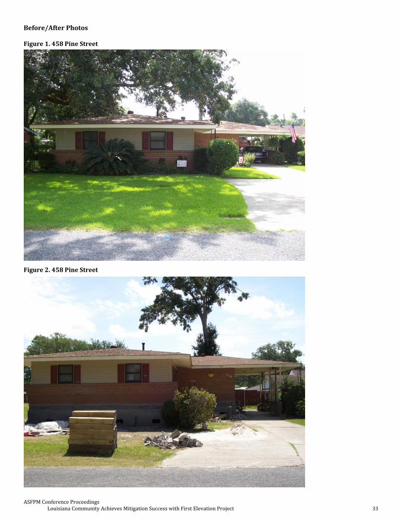
ASFPM Conference Proceedings Louisiana Community Achieves Mitigation Success with First Elevation Project 33

Before/After Photos Figure 1. 458 Pine Street

Figure 2. 458 Pine Street

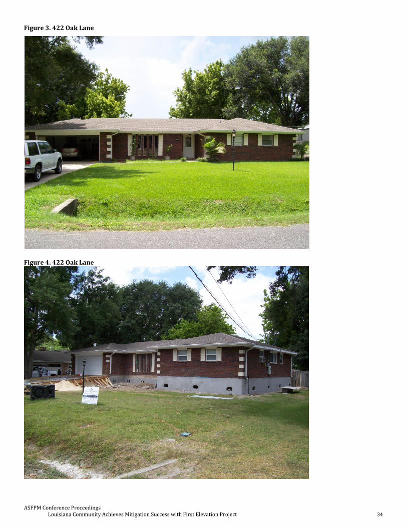
ASFPM Conference Proceedings Louisiana Community Achieves Mitigation Success with First Elevation Project 34

Figure 3. 422 Oak Lane

Figure 4. 422 Oak Lane

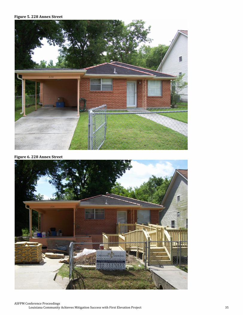
ASFPM Conference Proceedings Louisiana Community Achieves Mitigation Success with First Elevation Project 35

Figure 5. 228 Annex Street

Figure 6. 228 Annex Street

ASFPM Conference Proceedings Louisiana Community Achieves Mitigation Success with First Elevation Project 36

Figure 7. 130 Peter Lane

Figure 8. 130 Peter Lane

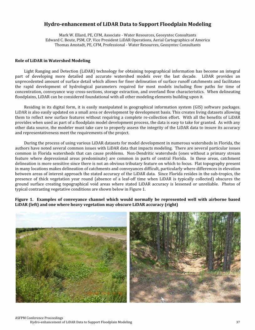
ASFPM Conference Proceedings Hydro-enhancement of LiDAR Data to Support Floodplain Modeling 37

Hydro-enhancement of LiDAR Data to Support Floodplain Modeling

Mark W. Ellard, PE, CFM, Associate - Water Resources, Geosyntec Consultants

Edward C. Beute, PSM, CP, Vice President LiDAR Operations, Aerial Cartographics of America Thomas Amstadt, PE, CFM, Professional - Water Resources, Geosyntec Consultants

Role of LiDAR in Watershed Modeling

Light Ranging and Detection (LiDAR) technology for obtaining topographical information has become an integral part of developing more detailed and accurate watershed models over the last decade. LiDAR provides an unprecedented amount of surface detail which allows for finer delineation of surface runoff catchments and facilitates the rapid development of hydrological parameters required for most models including flow paths for time of concentration, conveyance way cross-sections, storage extraction, and overland flow characteristics. When delineating floodplains, LiDAR can be considered foundational with all other modeling elements building upon it.

Residing in its digital form, it is easily manipulated in geographical information system (GIS) software packages.

LiDAR is also easily updated on a small area or development by development basis. This creates living datasets allowing them to reflect new surface features without requiring a complete re-collection effort. With all the benefits of LiDAR provides when used as part of a floodplain model development process, the data is easy to take for granted. As with any other data source, the modeler must take care to properly assess the integrity of the LiDAR data to insure its accuracy and representativeness meet the requirements of the project.

During the process of using various LiDAR datasets for model development in numerous watersheds in Florida, the

authors have noted several common issues with LiDAR data that impacts modeling. There are several particular issues common in Florida watersheds that can cause problems. Non-Dendritic watersheds (ones without a primary stream feature where depressional areas predominate) are common in parts of central Florida. In these areas, catchment delineation is more sensitive since there is not an obvious tributary feature on which to focus. Flat topography present in many locations makes delineation of catchments and conveyances difficult, particularly where differences in elevation between areas of interest approach the stated accuracy of the LiDAR data. Since Florida resides in the sub-tropics, the presence of thick vegetation year round (absence of a leaf-off time when LiDAR is typically collected) obscures the ground surface creating topographical void areas where stated LiDAR accuracy is lessened or unreliable. Photos of typical contrasting vegetative conditions are shown below in Figure 1. Figure 1. Examples of conveyance channel which would normally be represented well with airborne based LiDAR (left) and one where heavy vegetation may obscure LiDAR accuracy (right)

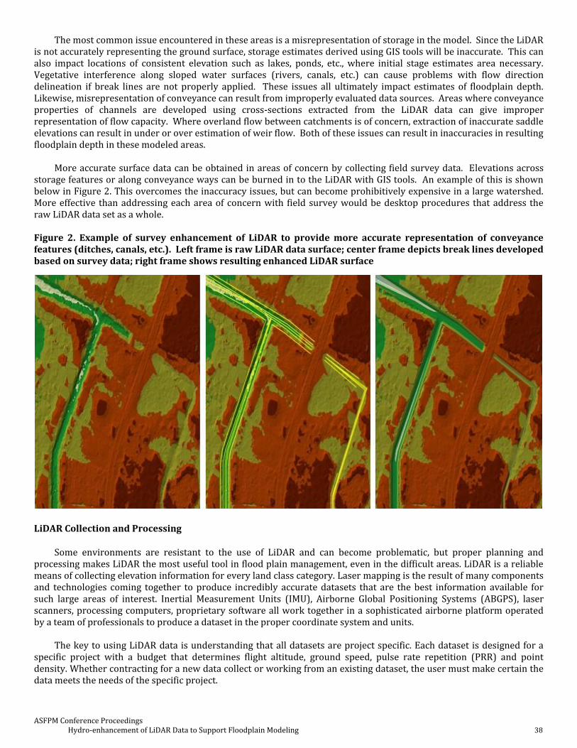
ASFPM Conference Proceedings Hydro-enhancement of LiDAR Data to Support Floodplain Modeling 38

The most common issue encountered in these areas is a misrepresentation of storage in the model. Since the LiDAR is not accurately representing the ground surface, storage estimates derived using GIS tools will be inaccurate. This can also impact locations of consistent elevation such as lakes, ponds, etc., where initial stage estimates area necessary. Vegetative interference along sloped water surfaces (rivers, canals, etc.) can cause problems with flow direction delineation if break lines are not properly applied. These issues all ultimately impact estimates of floodplain depth. Likewise, misrepresentation of conveyance can result from improperly evaluated data sources. Areas where conveyance properties of channels are developed using cross-sections extracted from the LiDAR data can give improper representation of flow capacity. Where overland flow between catchments is of concern, extraction of inaccurate saddle elevations can result in under or over estimation of weir flow. Both of these issues can result in inaccuracies in resulting floodplain depth in these modeled areas.

More accurate surface data can be obtained in areas of concern by collecting field survey data. Elevations across

storage features or along conveyance ways can be burned in to the LiDAR with GIS tools. An example of this is shown below in Figure 2. This overcomes the inaccuracy issues, but can become prohibitively expensive in a large watershed. More effective than addressing each area of concern with field survey would be desktop procedures that address the raw LiDAR data set as a whole. Figure 2. Example of survey enhancement of LiDAR to provide more accurate representation of conveyance features (ditches, canals, etc.). Left frame is raw LiDAR data surface; center frame depicts break lines developed based on survey data; right frame shows resulting enhanced LiDAR surface

LiDAR Collection and Processing

Some environments are resistant to the use of LiDAR and can become problematic, but proper planning and processing makes LiDAR the most useful tool in flood plain management, even in the difficult areas. LiDAR is a reliable means of collecting elevation information for every land class category. Laser mapping is the result of many components and technologies coming together to produce incredibly accurate datasets that are the best information available for such large areas of interest. Inertial Measurement Units (IMU), Airborne Global Positioning Systems (ABGPS), laser scanners, processing computers, proprietary software all work together in a sophisticated airborne platform operated by a team of professionals to produce a dataset in the proper coordinate system and units.

The key to using LiDAR data is understanding that all datasets are project specific. Each dataset is designed for a

specific project with a budget that determines flight altitude, ground speed, pulse rate repetition (PRR) and point density. Whether contracting for a new data collect or working from an existing dataset, the user must make certain the data meets the needs of the specific project.

ASFPM Conference Proceedings Hydro-enhancement of LiDAR Data to Support Floodplain Modeling 39

Classification Process

It is the classification process that adds additional information beyond the location of a point. Proper classification of LiDAR data can reveal whether a point belongs to a certain feature class such as ground, vegetation, structure, or water. Depending on the dataset and project needs, the classes to which points can be assigned is infinite. Automated classification is accomplished by subjecting the pre-processed data to a set of parameters where each point is analyzed to determine if it fits a specific condition and assigning that point to a group of like points. The benefit is that this can be accomplished with automated routines invoked in a batch processing mode. Small sections representative of the entire project should be tested in advance of the process to ascertain that the routine will produce the desired results. When acceptable results are achieved, the process can be launched to analyze the entire dataset.

A review of the data will reveal that automated routines classify most of the project correctly. Typically, 90-95% of

the data will be directed to the intended class. The remaining points have not been assigned because they did not meet the criteria defined in the routine. Points fall outside the parameters because of the large number of variables that are possible for each point making a completely automated classification unlikely. This leaves the remaining 5-10% to be classified using manual techniques where human intervention is necessary to locate those areas where the automated routines were unsuccessful. In this part of the process other classification tools are used to categorize the points to meet project expectations. It is a part of the Quality Control - Quality Assurance process and it is very labor intensive.

There are two common errors when classifying a dataset. The first is over-filtering the data. The result is data that

contains no artifacts and is very smooth. There is not a ripple to the ground data. The error in this case is that there is valuable information that has not been assigned to the class that can be useful to the end user. The data is not missing. It is in the point cloud usually in the unclassified or default class. The points often missed are the top of bank on conveyances and storage areas and other subtle drainage features. The second error is under-filtered data. This results in data that is very noisy. Artifacts in the form of low-lying vegetation have been included in the ground class. Modeling is compromised in both scenarios. Both of these datasets can be corrected with a fair amount of work. Given a preference, the over-filtered data will yield information easier than the under-filtered data. It is always easier to add data to the ground than it is to take it out of the ground data.

Typically, these issues are seen in areas of dense tree canopy where the ground is obscured. In open areas

drainage patterns are obvious and imagery can be used to solve these issues. It is not as simple in the areas that cannot be viewed with imagery. Image analysis may indicate the presence of a drainage pattern, but not reveal the ground or the actual location of the conveyance (Figure 3). Figure 3. Same area comparison of aerial imagery (left), LiDAR point surface representation (center), and example of classified LiDAR point cloud (right) with ground points in orange, unclassified areas in white, and estimated conveyance path in blue

LiDAR, however, is able to define both ground and drainage. Drainage features can be seen in a surface model with

the ground superimposed. It can be seen clearly in Figure 3 that the location of the conveyance is undetermined from the aerial (left frame). The over-filtered data in (showing ground in orange) reveals a wide area defining the conveyance (as seen in white). The white points are actually unclassified LiDAR points. They are points that did not meet the conditions set up in the automated routine parameter to be included in the ground class. At some point an attempt was made to locate the conveyance in the original data as represented by the blue line in the right frame of Figure 3.

ASFPM Conference Proceedings Hydro-enhancement of LiDAR Data to Support Floodplain Modeling 40

Following an enhancement of the data to include more points into the ground class through reclassification, there are noticeable differences in the surface as shown in Figure 4 below. Where there were no artifacts previously, the surface has now become noisy (as seen particularly in the northeast corner) due to the inclusion of some artifacts in the ground class. Previously the location of the conveyance was undetermined, now the location can be located very specifically. The difference in the surfaces is highlighted when the attempt to show the location of the conveyance from the old model is placed in the enhanced dataset. Better results are realized when the dataset is enhanced. Most datasets can be enhanced to reveal this level of detail. Figure 4. Comparison of raw LiDAR vs. Hydro-Enhancement of same area

Following are examples of LiDAR enhancement from existing datasets though reclassification. The white points in

the left frame of Figure 5 below are unclassified data not having met the criteria of the classification process. The orange points are those that have been classified as ground. The figures show clearly the added value from the enhancement. In the left frame of Figure 5 the surface definition is unacceptable due to the few number of ground points. Following enhancement, the right frame of Figure 5 shows a sufficient number of points added to the ground class to properly represent the surface. Figure 5. Profile view comparison of classified LiDAR points of same area – orange points classified as ground, white points classified as non-ground points

ASFPM Conference Proceedings Hydro-enhancement of LiDAR Data to Support Floodplain Modeling 41

The surface models in Figure 6 demonstrate improvements using enhancement classification techniques where

blue represents the lowest elevation and red the highest. While the data is noisy following the process, conveyances that were once blocked due to erroneous data are now open allowing proper modeling of the data. Figure 6. Comparison of raw LiDAR vs. Hydro-Enhancement of same area

All existing datasets should be examined before use to determine suitability for a project by identifying any holidays, voids, and point density. One should also consider enhancement of the data through reclassification to obtain additional ground points, identify structures and separate vegetation by height. Breaklines should always be included to hydro-enforce the data for the best surface model quality. Breaklines can be collected many ways including field surveys photogrammetry, stereo-imagery, Lidargrammetry, or through direct terrain extraction techniques where the breakline elevation and position are taken from the laser points using QCoherent LP360 or Cardinal Systems VrLiDAR software.

Modeling Results Impact

Enhancement of LiDAR has benefitted watershed modeling efforts by providing more accurate representation of storage and conveyance features. An example which benefitted from hydro-enhancement procedures is shown in Figure 7. This is a particular catchment area has flat topography and a channel feature shrouded with dense vegetation. Hydro-enhancement procedures were applied to the original LiDAR data set to better classify the points for hydrologic and hydraulic model representation.

Figure 7. Example model area – red outline delineates catchment boundary, blue lines channel location, and green stations cross-section locations

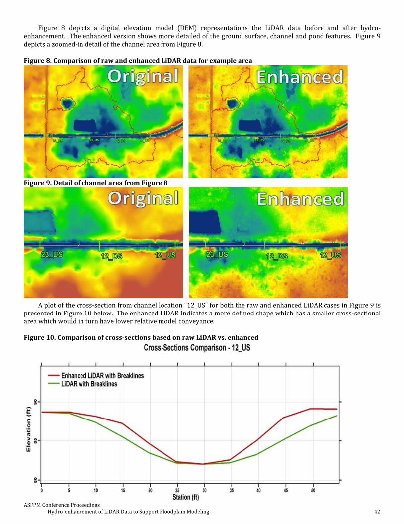
ASFPM Conference Proceedings Hydro-enhancement of LiDAR Data to Support Floodplain Modeling 42

Figure 8 depicts a digital elevation model (DEM) representations the LiDAR data before and after hydro-enhancement. The enhanced version shows more detailed of the ground surface, channel and pond features. Figure 9 depicts a zoomed-in detail of the channel area from Figure 8. Figure 8. Comparison of raw and enhanced LiDAR data for example area

Figure 9. Detail of channel area from Figure 8

A plot of the cross-section from channel location “12_US” for both the raw and enhanced LiDAR cases in Figure 9 is presented in Figure 10 below. The enhanced LiDAR indicates a more defined shape which has a smaller cross-sectional area which would in turn have lower relative model conveyance. Figure 10. Comparison of cross-sections based on raw LiDAR vs. enhanced

ASFPM Conference Proceedings Hydro-enhancement of LiDAR Data to Support Floodplain Modeling 43

The impact on modeling in this example is an increase in modeled flood stage using the enhanced LiDAR dataset representing a higher flood risk. This is shown in Figure 11. Figure 11. Model flood stage comparison: red based on enhanced data, blue original data

Conclusions

LiDAR plays a foundational role in today’s floodplain modeling efforts. The detailed topographical representation that LiDAR brings allows for increased accuracy and detail to be added to floodplain models, while expending less effort and budget than traditional model parameterization techniques. The modeler should take care and properly review the LiDAR sets, however, to ensure they meet the needs of the project. Proper classification of ground points is critical to accurately define conveyance ways and represent storage. Where issues arise with LiDAR accuracy through point misclassification in areas with dense vegetation along hydrographic features, hydro-enhancement of the LiDAR data set using the methods discussed in this paper helps to improves surface representation. This enhancement in turn leads to better model representation and increases floodplain delineation accuracy in these areas.

ASFPM Conference Proceedings Case Study on Impacts of Evolving Nearshore Bathymetry and Topography on Base Flood Elevations and Implications for Stakeholders 44

Case Study on Impacts of Evolving Nearshore Bathymetry and Topography on Base Flood Elevations and Implications for Stakeholders

D. Michael Parrish

Greenhorne & O'Mara, Inc.

Introduction

We present a case study of impacts of evolving nearshore bathymetry and topography on base flood elevations and provide a discussion of implications from various perspectives. The example site is located in Pacific County, Washington, on Long Beach. The sandy shore there is exposed to the Pacific Ocean. Some of the limitations of flood insurance rate maps are exposed and discussed.

Methodology

We simulated several flood and high wave events and estimated erosion effects as detailed below. We selected wave events based upon maximum hourly wave heights as received from the National Data Buoy Center for station 46029 (NDBC, 2011). A simple computer code assessed hourly wave heights by calculating the time between a given wave height and the nearest higher wave height. The code selected wave heights at least seven days apart from any greater wave height. For example, the highest hourly wave height is 13.8 m (45.3 ft). The next highest hourly wave height is 12.8 m (42.0 ft), and, since it occurred more than 7 days before the greater wave height, the 12.8 m wave height is accepted as an independent event. On the other hand, an 11.8 m (38.7 ft) wave height occurred only three hours after the previous wave height of 13.8 m, and is therefore excluded from the scenarios. 7 days was selected as the threshold in order to generate about 20 events per year for 15 years. We utilized the nearshore profile data presented in Ruggerio et al. (2007). They provide beach profiles for eight consecutive years, from the spring of 1998 to spring 2005 (Figure 1). In general, there appears to be an accretion of sand: the beach profile is moving seaward. We estimated beach slopes from these data for use in estimates of beach erosion (slopes—run over rise—vary from 34 to 50). Median grain size data for the same years, collected as part of their study, were also useful to us; the grain size parameter is needed for the erosion methodology employed (MK&A; FEMA, 2004). Our data source for water levels are the records for station 9440910, maintained by the National Atmospheric and Oceanographic Administration’s Tides and Currents program (NOAA, 2011). We computed runup according to the direct integration method (DIM; FEMA, 2004) and estimated storm duration as the time between wave heights that are half the peak wave height (i.e., full width at half maximum, FWHM).

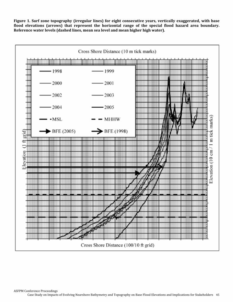
ASFPM Conference Proceedings Case Study on Impacts of Evolving Nearshore Bathymetry and Topography on Base Flood Elevations and Implications for Stakeholders 45

Figure 1. Surf zone topography (irregular lines) for eight consecutive years, vertically exaggerated, with base flood elevations (arrows) that represent the horizontal range of the special flood hazard area boundary. Reference water levels (dashed lines, mean sea level and mean higher high water).

ASFPM Conference Proceedings Case Study on Impacts of Evolving Nearshore Bathymetry and Topography on Base Flood Elevations and Implications for Stakeholders 46

Results Base flood elevations in this case are runup elevations. After rounding, all base flood elevations are 12 ft, except for the one developed with the 1998 topography, which is 13 ft. Although there was not much difference among the BFE’s computed using the various topographic data sets, there is a noticeable difference among the various horizontal runup extents. The extent of runup ranges about 60 m (200 ft) among the topographic datasets applied. This is significant at the typical map scales applied to flood insurance rate maps (FIRM’s; e.g., 1:6000). The effects of erosion in this case would seem not to modify the topography, since the actual dunes lie landward of what would otherwise be the toe of the eroded dune. In summary: at this location, for the period 1998 through 2005, the base flood elevations are fairly stable, while the boundary of the special flood hazard area is moving seaward. Discussion We would now present some of the implications of the foregoing results for the consideration of the reader. This cannot be an exhaustive account, but is meant to highlight some of the issues that we see and is meant to prompt further discussion.

Emergency planners may be interested to understand how coastal flood threats are changing depending upon beach configuration. As beach profiles change, the potential for actual coastal hazards also changes. In the case presented above, the hazard appears to be declining with time. This may prompt adjustments in emergency plans, as resources and attention are shifted to geographic areas more prone to hazards. And hazards here include not only coastal flooding but other natural and man-made hazards as well (e.g., fire, earthquake). We imagine a hypothetical situation where the beach continues to experience accretion and therefore the coastal flood hazard may become essentially negligible in comparison to other potential hazards. Many coastal flood studies begin with the collection of LiDAR or survey data on which to base the flood hazard calculations. The studies’ contract documents may specify that LiDAR from a specific year be implemented. We understand that this is meant to provide for the estimation of existing conditions to be mapped. However, as many studies require multiple years between the first proposed scope and acceptance by the affected communities, the corresponding flood hazard rate maps may already be out of date by the time they become effective. The value of conducting a new survey for a new study or of accepting the result of such a survey (even after quality control) verbatim, without consideration for temporal effects is debatable. Put another way, if there is not much change in topography, conducting a new survey seems unnecessary. On the other hand, if the topography is changing relatively rapidly, the use of a single survey is inconsistent with reality. It may be more respectful of the available data to estimate future (e.g., at the time of the effective date) conditions based upon multiple surveys. At present, FIRM’s are created based upon what are assumed to be existing conditions. These maps may be effective for decades before the same areas are restudied. In the interim, the hazards may change but the associated maps and insurance rates remain constant. Our example illustrates a case where this might result in overcharging a policy holder, as, for example, the special flood hazard area may move from landward of the owner’s residence to somewhere seaward of the residence. The inability to represent the dynamic extent of inundation on a static map may also result in financial difficulties in the converse case—that is, under representing risk on the FIRM may result in claims and expenses that exceed the premiums. Ideally, this will average out. But consider that the map revision process provides a disincentive to update maps where the affected parties would be shown to lie in regions more hazardous than previously thought. Letters of map change tend to be requested when the property owner can be shown to have less (even zero) financial obligation toward the National Flood Insurance Program than when flood insurance cost can be demonstrated to be increasing. Conversely, the property owner may have a disproportionate financial burden placed upon him or her in the case highlighted herein. The threat of hazardous wave action is moving seaward, but the map fails to communicate this.

ASFPM Conference Proceedings Case Study on Impacts of Evolving Nearshore Bathymetry and Topography on Base Flood Elevations and Implications for Stakeholders 47

Builders are charged with constructing structures that are intended to last decades. In an area where the flood hazards are changing significantly from year to year, the builder stands to lose regardless of whether the flood hazard is moving seaward or landward. If the hazard is moving landward, the problem is that the builder’s customer, having trusted the builder’s judgment in the siting of the structure, stands to be disappointed when the corresponding FIRM is revised or when a significant event affects the site. If the hazard is moving seaward, the builder has the potential for opportunity cost. Significant movement seaward of the coastal high hazard area, for example, might make room for additional rows of structures in the seaward direction (perhaps two rows of residences could fit within the 200 ft shift of our example), and thus additional profit for the builder. However, this additional profit might be unavailable to him or her depending upon the timing of the construction project. Location of the site relative to the coastal high hazard area also impacts costs of construction, as various building codes may come into play according to the relative site location. Floodplain managers may utilize FIRM’s in making decisions about how to best utilize the flood plain resource and about how to protect the public from potential disasters. However, an outdated FIRM may contain misinformation or disinformation about the location of the extent of the base flood.

Acknowledgements

Thanks to Mary Searing and Dan Saltsman of Greenhorne & O'Mara, Inc. for reviewing drafts of this paper and the corresponding presentation.

References

Ruggerio P et al. (2007) Beach Morphology Monitoring in the Columbia River Littoral Cell: 1997–2005. USGS Data Series 260. http://pubs.usgs.gov/ds/2007/260/

NOAA (2011) Tides and Currents. http://tidesandcurrents.noaa.gov NDBC (2011) National Data Buoy Center. http://www.ndbc.noaa.gov

FEMA (2004) Guidelines and Specifications for Flood Hazard Mapping Partners. Appendix D.4: Coastal Flooding Analyses and Mapping: Pacific Coast.

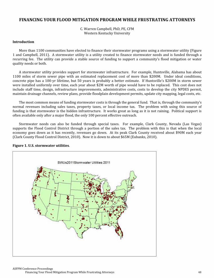
ASFPM Conference Proceedings Financing Your Flood Mitigation Program While Frustrating Attorneys 48

FINANCING YOUR FLOOD MITIGATION PROGRAM WHILE FRUSTRATING ATTORNEYS

C. Warren Campbell, PhD, PE, CFM Western Kentucky University

Introduction

More than 1100 communities have elected to finance their stormwater programs using a stormwater utility (Figure 1 and Campbell, 2011). A stormwater utility is a utility created to finance stormwater needs and is funded through a recurring fee. The utility can provide a stable source of funding to support a community’s flood mitigation or water quality needs or both.

A stormwater utility provides support for stormwater infrastructure. For example, Huntsville, Alabama has about 1100 miles of storm sewer pipe with an estimated replacement cost of more than $200M. Under ideal conditions, concrete pipe has a 100-yr lifetime, but 50 years is probably a better estimate. If Huntsville’s $200M in storm sewer were installed uniformly over time, each year about $2M worth of pipe would have to be replaced. This cost does not include staff time, design, infrastructure improvements, administrative costs, costs to develop the city NPDES permit, maintain drainage channels, review plans, provide floodplain development permits, update city mapping, legal costs, etc.

The most common means of funding stormwater costs is through the general fund. That is, through the community’s normal revenues including sales taxes, property taxes, or local income tax. The problem with using this source of funding is that stormwater is the hidden infrastructure. It works great as long as it is not raining. Political support is often available only after a major flood, the only 100 percent effective outreach.

Stormwater needs can also be funded through special taxes. For example, Clark County, Nevada (Las Vegas) supports the Flood Control District through a portion of the sales tax. The problem with this is that when the local economy goes down as it has recently, revenues go down. At its peak Clark County received about $90M each year (Clark County Flood Control District, 2010). Now it is down to about $65M (Eubanks, 2010). Figure 1. U.S. stormwater utilities.

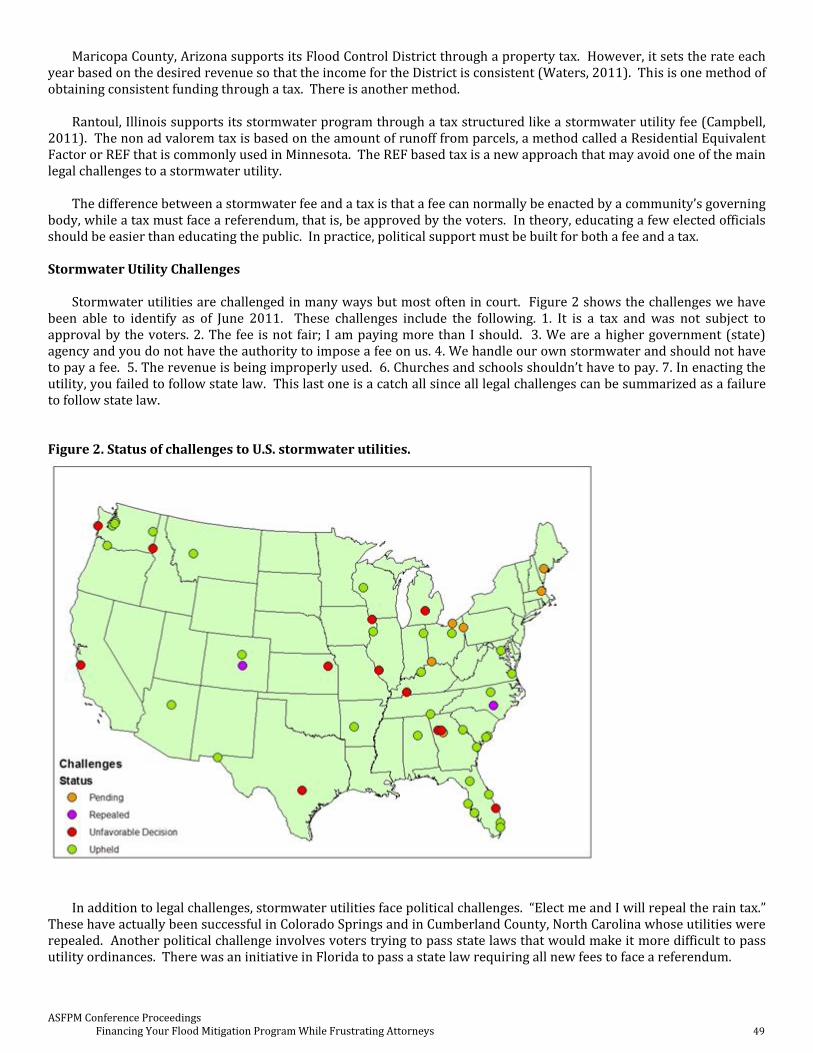
ASFPM Conference Proceedings Financing Your Flood Mitigation Program While Frustrating Attorneys 49

Maricopa County, Arizona supports its Flood Control District through a property tax. However, it sets the rate each year based on the desired revenue so that the income for the District is consistent (Waters, 2011). This is one method of obtaining consistent funding through a tax. There is another method.

Rantoul, Illinois supports its stormwater program through a tax structured like a stormwater utility fee (Campbell, 2011). The non ad valorem tax is based on the amount of runoff from parcels, a method called a Residential Equivalent Factor or REF that is commonly used in Minnesota. The REF based tax is a new approach that may avoid one of the main legal challenges to a stormwater utility.

The difference between a stormwater fee and a tax is that a fee can normally be enacted by a community’s governing body, while a tax must face a referendum, that is, be approved by the voters. In theory, educating a few elected officials should be easier than educating the public. In practice, political support must be built for both a fee and a tax. Stormwater Utility Challenges

Stormwater utilities are challenged in many ways but most often in court. Figure 2 shows the challenges we have been able to identify as of June 2011. These challenges include the following. 1. It is a tax and was not subject to approval by the voters. 2. The fee is not fair; I am paying more than I should. 3. We are a higher government (state) agency and you do not have the authority to impose a fee on us. 4. We handle our own stormwater and should not have to pay a fee. 5. The revenue is being improperly used. 6. Churches and schools shouldn’t have to pay. 7. In enacting the utility, you failed to follow state law. This last one is a catch all since all legal challenges can be summarized as a failure to follow state law.

Figure 2. Status of challenges to U.S. stormwater utilities.

In addition to legal challenges, stormwater utilities face political challenges. “Elect me and I will repeal the rain tax.” These have actually been successful in Colorado Springs and in Cumberland County, North Carolina whose utilities were repealed. Another political challenge involves voters trying to pass state laws that would make it more difficult to pass utility ordinances. There was an initiative in Florida to pass a state law requiring all new fees to face a referendum.

ASFPM Conference Proceedings Financing Your Flood Mitigation Program While Frustrating Attorneys 50

A recent unique challenge involved an opinion by the Attorney General of Georgia who was asked by the State Department of Transportation to review the requirement of the DOT to pay fees to the Douglas County stormwater utility. Inexplicably, he found that the DOT should not have to pay the fee. Later in accordance with this opinion, the state Department of Agriculture informed Garden City that they would not be paying their stormwater fee. Garden City, in accordance with its stormwater ordinance, informed the Department of Agriculture that they would be turning off their water and sewer if the bill was not paid in full. The Agriculture Department then decided to pay the fee and the Attorney General seemed to reverse himself, although this is unclear (Johnson, et al. 2009, and Ecological Solutions, Inc., 2010).

It is difficult to understand how an Attorney General could publish an opinion finding that state agencies are not

subject to utility bills. As far back as 1997, the Florida Attorney General gave the opposite opinion (Office of the Attorney General of Florida, 1997). Obviously, statutes differ from state to state. In the case of the Douglas County utility, their ordinance stated that non-payment resulted in a lien against the property. Since they could not place a lien against public land, their only option was a civil suit. By contrast, Garden City’s ordinance allowed the denial of water and sewer service which provided more leverage against the Georgia Agriculture Department. This ordinance gave leverage that the Douglas County ordinance lacked. The conclusion is obvious; write ordinances that give immediate leverage.

The question of Federal agencies being subject to stormwater fees was settled with a new Federal law which appears to make Federal agencies across the country subject to millions in unpaid fees. The bill states that reasonable charges for stormwater services are fees and not taxes, and Federal agencies are subject to them (ASFPM, 2011). Stormwater Utility Fee Systems

One way in which utilities are challenged is to claim fees are unfairly distributed. Several methods are used to establish fees: 1) flat fees for all properties, 2) based on the number and sizes of water meters, 3) tier fees based on ranges of impervious surface, 4) fees based on the Equivalent Residential Unit (ERU) method, and 5) fees based on the Residential Equivalent Factor (REF).

Tier systems break non-residential property into ranges of impervious surface. Each property pays the same fee as other properties in the same tier. If the monthly fee for a tier system is plotted against property impervious surface, an increasing stair step function results (Figure 3). Tier systems can be made fair but often are not. This will be discussed in more detail after we introduce the ERU.

An ERU is usually the average impervious area of a single family residential property. It is estimated by sampling single family residential properties in the community and averaging the impervious area. In the U.S., the average ERU is about 3,000 sq ft (Campbell, 2011). For nonresidential properties, the fee is based on the ratio of parcel impervious area to the ERU. If a Walmart has 300,000 sq ft of impervious surface in a town with an ERU fee of $4 per month, then the Walmart will pay $400 per month. An ERU system is basically a tier system with an infinite number of tiers (Reese, 2010).

Tier systems are subject to political gerrymandering. Figure 3 provides an example of a tier system that could be improved for better agreement with the ERU fee. In this example, the assumed ERU of the community is 3200 sq ft and a $3 per monthly base fee is assumed. The chart plots tier and ERU fees as a function of parcel impervious area. From the chart, very large parcels benefit from the tier fee. In this tier fee system, small and medium-sized businesses will pay disproportionately higher fees than they would under an ERU system.

The fee system can be improved using two systems. The first, shown in Figure 4, minimizes the maximum absolute

deviation from the ERU fee within a tier. To obtain the best absolute error tier system, the ERU fee curve should pass through the midpoint of each tier. In an optimum tier system, the maximum error is given by Equation 1.

(1)2

$3where

3200

difference in impervious areas of the upper and lower bounds of the tier

k IAMaximum Error

k

IA

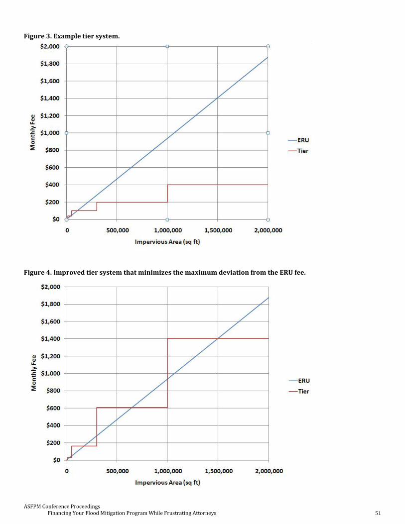
ASFPM Conference Proceedings Financing Your Flood Mitigation Program While Frustrating Attorneys 51

Figure 3. Example tier system.

Figure 4. Improved tier system that minimizes the maximum deviation from the ERU fee.

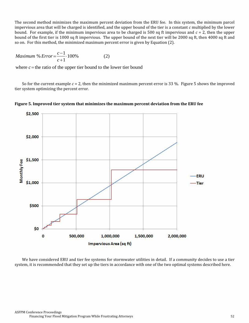
ASFPM Conference Proceedings Financing Your Flood Mitigation Program While Frustrating Attorneys 52

The second method minimizes the maximum percent deviation from the ERU fee. In this system, the minimum parcel impervious area that will be charged is identified, and the upper bound of the tier is a constant c multiplied by the lower bound. For example, if the minimum impervious area to be charged is 500 sq ft impervious and c = 2, then the upper bound of the first tier is 1000 sq ft impervious. The upper bound of the next tier will be 2000 sq ft, then 4000 sq ft and so on. For this method, the minimized maximum percent error is given by Equation (2).

1% 100% (2)

1

where the ratio of the upper tier bound to the lower tier bound

cMaximum Error

c

c

So for the current example c = 2, then the minimized maximum percent error is 33 %. Figure 5 shows the improved tier system optimizing the percent error. Figure 5. Improved tier system that minimizes the maximum percent deviation from the ERU fee

We have considered ERU and tier fee systems for stormwater utilities in detail. If a community decides to use a tier

system, it is recommended that they set up the tiers in accordance with one of the two optimal systems described here.

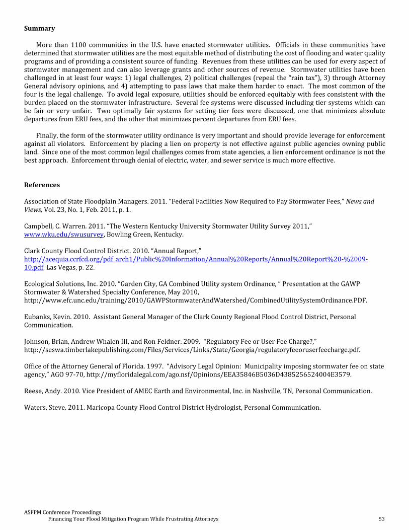
ASFPM Conference Proceedings Financing Your Flood Mitigation Program While Frustrating Attorneys 53

Summary

More than 1100 communities in the U.S. have enacted stormwater utilities. Officials in these communities have determined that stormwater utilities are the most equitable method of distributing the cost of flooding and water quality programs and of providing a consistent source of funding. Revenues from these utilities can be used for every aspect of stormwater management and can also leverage grants and other sources of revenue. Stormwater utilities have been challenged in at least four ways: 1) legal challenges, 2) political challenges (repeal the “rain tax”), 3) through Attorney General advisory opinions, and 4) attempting to pass laws that make them harder to enact. The most common of the four is the legal challenge. To avoid legal exposure, utilities should be enforced equitably with fees consistent with the burden placed on the stormwater infrastructure. Several fee systems were discussed including tier systems which can be fair or very unfair. Two optimally fair systems for setting tier fees were discussed, one that minimizes absolute departures from ERU fees, and the other that minimizes percent departures from ERU fees.

Finally, the form of the stormwater utility ordinance is very important and should provide leverage for enforcement

against all violators. Enforcement by placing a lien on property is not effective against public agencies owning public land. Since one of the most common legal challenges comes from state agencies, a lien enforcement ordinance is not the best approach. Enforcement through denial of electric, water, and sewer service is much more effective.

References Association of State Floodplain Managers. 2011. “Federal Facilities Now Required to Pay Stormwater Fees,” News and Views, Vol. 23, No. 1, Feb. 2011, p. 1. Campbell, C. Warren. 2011. “The Western Kentucky University Stormwater Utility Survey 2011,” www.wku.edu/swusurvey, Bowling Green, Kentucky. Clark County Flood Control District. 2010. “Annual Report,” http://acequia.ccrfcd.org/pdf_arch1/Public%20Information/Annual%20Reports/Annual%20Report%20-%2009-10.pdf, Las Vegas, p. 22. Ecological Solutions, Inc. 2010. “Garden City, GA Combined Utility system Ordinance, “ Presentation at the GAWP Stormwater & Watershed Specialty Conference, May 2010, http://www.efc.unc.edu/training/2010/GAWPStormwaterAndWatershed/CombinedUtilitySystemOrdinance.PDF. Eubanks, Kevin. 2010. Assistant General Manager of the Clark County Regional Flood Control District, Personal Communication. Johnson, Brian, Andrew Whalen III, and Ron Feldner. 2009. “Regulatory Fee or User Fee Charge?,” http://seswa.timberlakepublishing.com/Files/Services/Links/State/Georgia/regulatoryfeeoruserfeecharge.pdf. Office of the Attorney General of Florida. 1997. “Advisory Legal Opinion: Municipality imposing stormwater fee on state agency,” AGO 97-70, http://myfloridalegal.com/ago.nsf/Opinions/EEA35846B5036D4385256524004E3579. Reese, Andy. 2010. Vice President of AMEC Earth and Environmental, Inc. in Nashville, TN, Personal Communication. Waters, Steve. 2011. Maricopa County Flood Control District Hydrologist, Personal Communication.

ASFPM Conference Proceedings Fort Worth Roadway Flood Hazard Assessment 54

Fort Worth Roadway Flood Hazard Assessment

Steven E. Eubanks, P.E., CFM, City of Fort Worth Rich DeOtte, P.E., CFM, DeOtte, Inc.

Background

Due to flash flooding associated with sudden thunderstorms, every year in Texas motorists drown from driving into high water and being swept off the road. Many more are rescued, and countless lucky ones never leave the road, but just have their vehicles stalled and have to wait for a tow truck to pull them out. There have been many debates about how to prevent these incidents, from barricades to flashers to gates to hefty fines for water rescues. After two fatal incidents in 2000 and 2001, the City of Fort Worth opted to try a flasher system which would activate when a roadway was overtopped and shut off when the road was clear again. Due to budget, maintenance, and reliability concerns, the City elected not to install automatic gates also, but to rely on flashers only to warn motorists of the hazard ahead. A pilot system was installed at three locations in far east Fort Worth based on past fatalities and a long response time for City crews to arrive with barricades.

The flasher system equipment was obtained from High Sierra Electronics and consists of a pressure transducer at

each crossing connected to a nearby base station in a standpipe. These are programmed to go off when water begins overtopping the roadway, sending a radio signal to the flashers and an ALERT message to the base station. The base station then sends out a text or e-mail message to key personnel. A similar signal and messages are sent when water drops back below the roadway. All remote components are solar powered and all locations can be queried from the base station.

Figure 1. Vehicles continually drive into high water on one frequently overtopped roadway with a flasher and previous fatalities, even after barricades have been placed. Five vehicles stalled out here when Tropical Storm Hermine dropped six inches of rain on September 8, 2010, but all riders made it out safely.

ASFPM Conference Proceedings Fort Worth Roadway Flood Hazard Assessment 55

In early 2004 Fort Worth voters approved a bond election which had among other things $500,000 for expansion of the High-Water Warning System, which would fund installation at about fifteen additional crossings. Five fatalities at two low-water crossings on April 30 and June 2 caused system expansion to become a top priority. Identifying the most hazard locations to install these became a pressing issue. City staff began with a list of 32 locations used by Field Operations staff for frequent barricading, and a local consultant, DeOtte, Inc., was selected to help staff to rate these sites. Soon thereafter, a 1993 in-house study was made available (performed in response to previous flash flood fatalities) in which police and fire personnel identified over 700 locations within Fort Worth where they had experienced high water at some time in the past. City staff began comparing these locations to the FEMA Flood Insurance Rate Maps and to profiles in the accompanying Flood Insurance Study, removing duplicate locations as well as adding locations from newly annexed areas on the outskirts of town. This list was eventually pared down to a list of 285 potentially hazardous flood-prone roadway crossings, of which the first 32 locations were being assessed in the initial phase.

The Assessment

DeOtte, Inc., developed a preliminary ranking system based on eight (8) criteria which they determined were essential in assessing the hazard at a particular crossing. A scoring system was set up for each criterion, and the system was finalized after input from City staff. Subsequently, city staff identified a ninth criterion (detour length) which was added to the rating system. For presentation purposes, these have been organized into three groups: objective criteria, historical incident criteria, and judgment criteria. Objective Criteria These criteria are all determined by calculated or empirical data and are the initial basis for determining the likely hazard at a particular roadway crossing.

1. Depth of Water over Roadway: The greater the depth, the greater the likelihood that a vehicle could leave the

roadway or be inundated with persons inside. Overtopping depths were estimated from the FIS or other available studies, from physical evidence at the crossing, or by using best judgment based on rough hydrology and estimated culvert or bridge capacity. Depths from routine, 5-year and 10-year storms were considered in addition to 100-year depth. Scoring: Overtopping over three feet = 10 points; one to three feet = 8 points, and less than one foot = 5 points.

2. Frequency of Overtopping: Higher frequency overtopping lead to more opportunities for drivers to enter high

water. Although one would expect that with increased frequency drivers would become more aware of the hazard, repeated incidents in urban settings have demonstrated that that expectation is false. Overtopping frequency was estimated from the same information as the previous criterion. Scoring: Very frequent (more than once per year) = 10 points; frequent (every 1-5 years) = 5 points; infrequent (10-100-year storm) = 1 point.

3. Traffic Volumes: Although it is obvious that higher traffic volumes represent a greater chance of an incident, in

some cases it also leads to a higher expectations of safety from the traveling public. Further, in developing areas on the outskirts of town, many new residents used to urban conditions are not as expectant of undersized crossings common on rural roads (now with significantly more traffic) and so have a greater likelihood of driving into high water. Where traffic counts were not available, estimates were made during field inspection based on level of traffic and time of day. Scoring: Over 5000 vehicles per day (vpd) = 10 points; 1000-5000 vpd = 5 points; 500-1000 vpd = 3 points; less than 500 vpd = 1 point.

Historical Incident Criteria Actual incidents and reports at a site are not only an indication of true risk, but also raise public expectations for a response by local government.

4. Past Fatalities: That a fatality has occurred as a site documents that a risk exists independent of other factors. Every location with a fatal incident is given full points. Fortunately, no location in over 25 years of available records has had more than one fatal incident, although several incidents resulted in multiple fatalities. Scoring: One or more known fatalities = 10 points.

5. High Water Rescues: A rescue also documents that a genuine risk is present at a site, although without the tragedy of a fatality. Unfortunately, a number of sites have had multiple rescues. Available fire department records were reviewed to identify rescues in recent years. Scoring: 5 points per known rescue, up to a maximum of 20 points.

ASFPM Conference Proceedings Fort Worth Roadway Flood Hazard Assessment 56

Figure 2. Although seventeen people have lost their lives in Fort Worth since 1986 in roadway flooding incidents, countless others such as this young man who drove this car into high water have escaped unharmed.

6. Citizen Calls: Calls by citizens about hazardous conditions must be considered as a sign of genuine risk and in some cases avoided catastrophes. Some locations, however, are called in numerous times by citizens, while others, likely as dangerous or more so, are never reported. Scoring: ½ point per complaint, up to a maximum of 10 points. Judgment Criteria The last three criteria are indented to address intangible judgment factors that reflect either the likelihood for a driver to enter high water or the consequences if one did. These criteria were considered critical for discriminating among dangerous locations to find the ones likely most hazardous to drivers in the city.

7. Hazard Concealment: This criterion is the most difficult to explain and can be in some instances counter-intuitive. A crossing that looks extremely dangerous is more likely to be recognized as a hazard by drivers and less likely to be entered. In that light, most flood-related deaths result from a driver’s failure to recognize the hazard. This criterion assesses how concealed a hazard might be, either due to lack of lighting in a remote area or due to deceptive conditions such as smooth waters. Typically guard rails or other obstructions which create turbulence provide more visual clues to hazardous fast-moving water. An additional hazard relates to railroad overpasses, in which the roadway often has a pronounced sump as it dips below it. In one tragic accident in 1986, a vehicle stalled in high water under a railroad overpass and a mother and child who exited the vehicle to wade out were then sucked into inlets and drowned. Rating this can be difficult, and in several instances scores were re-assessed using the consensus judgment of at least two reviewers. Scoring: Still or hard-to-see water, or railroad overpass = 10 points; moving water but doesn’t look too bad = 7 points; crossing looks dangerous = 2 points.

8. Flooding or Downstream Threat: The consequences of a vehicle entering the water is also considered in hazard

assessment. An incised channel or steep drop-off represents an extremely dangerous condition for any vehicle leaving the roadway. Downstream vegetation may catch a floating vehicle, but may be as likely to cause it to submerge quickly under a limb. A vehicle floating into a roadside ditch contributed to at least one fatality in recent years. In other cases floodwaters spread so wide and shallow that a vehicle would likely stall out while still in slow-moving backwaters, reducing the threat to the vehicle or passengers. This can also be the case when the roadway is rather level, so that it acts as a shallow weir with reduced depth and velocity. In some situations—such as the railroad overpass condition described above—threat to a stalled vehicle still in the roadway must be considered. Rating this threat is subjective and in some cases may need to be determined by a consensus of opinion. Scoring: 50% or greater likelihood of a fatality = 10 points; 10%-50% = 8 points; less than 10% = 2 points.

ASFPM Conference Proceedings Fort Worth Roadway Flood Hazard Assessment 57

Figure 3. This railroad underpass was the site of two fatalities in 1986.

9. Detour Length: This criterion was developed to consider the driver’s inconvenience or impatience. A review

after the initial assessment indicated that a number of fatalities or rescues occurred in locations where a long detour would have been required. Rather than backtracking and going a long distance out of the way, some drivers appeared to be more willing to try to cross high water. Although distance rather than travel time was used, both could be considered. Scoring: Detour length greater than one-half mile = 10 points; 3 blocks to one-half mile = 8 points; less than 3 blocks = 1 point.

The Results

Based on the assessment of the original 32 locations, fifteen additional High-Water Warning Systems were installed, bringing the City’s total to eighteen. Subsequently the remaining 253 sites were assessed, some by an engineering intern working for the City and some by the consultant. DeOtte, Inc., performed a field review of the intern’s work to ensure consistency of judgment. Before selecting the highest ranking sites, City staff visited high-scoring locations to verify or modify factors such as Hazard Concealment and Downstream Threat. A two-page inspection form (available from the author) was used on each site, and the form, photos, FEMA profiles and related materials were assembled as hard copies into notebooks for future reference. Based on these rankings, a total of 30 additional High-Water Warning Systems are currently being installed to protect 38 crossings (several are so close to each other that a single transducer can be shared).

Future work includes upgrading several high-ranking crossings with capital improvement projects currently either

in planning or under design. Fort Worth is also in the beginning stages of developing a flood warning system. Two flasher sites already have complete weather stations, several more have rain gauges, and the rain gauge network is planned for expansion in the near future. In addition, lake level monitors are in use at several lakes, including on a 97-year-old city water supply lake with numerous homes around it subject to periodic flooding.

In spite of all of the flasher systems and in spite of roadways barricaded by city crews, drivers continue to enter high

water on a regular basis. Fort Worth has had seventeen fatalities since 1986, and the nine fatalities since 1996 place it second only to Bexar County (San Antonio) in Texas. Only one fatality has occurred since 2004, when Fort Worth began promoting the National Weather Service’s “Turn Around Don’t Drown” campaign. Ultimately it appears that targeting this program toward school children and young drivers may do more than any warning system to educate drivers to the danger of flooded roadways.

ASFPM Conference Proceedings 2-D Modeling as a Calibration Tool for Riverine Floodplain Analysis in the Front Range of Colorado 58

2-D Modeling as a Calibration Tool for Riverine Floodplain Analysis in the Front Range of Colorado

Alan D. Turner, P.E., CFM- CH2M HILL Engineers, Inc. Cory Hooper, P.E., CFM - CH2M HILL Engineers, Inc.

Introduction

In the front range of Colorado, stream channels are generally well channelized and confined to within the channel overbanks. However, in many cases floodplain encroachment, manmade structures, short reaches of stream, and alluvial fans exhibit multiple flow paths that are difficult to accurately model with typical 1-dimensional (1-D) models utilizing lateral weirs, inline weirs and flow junctions. 2-dimensional (2-D) models can quickly represent multiple flow paths, peak flows and flow quantity for each flow path. However, 2-D modeling can cause many problems as a standalone model. Regulatory issues surround 2-D models that can make them difficult to incorporate into existing Federal Emergency Management Agency (FEMA) regulatory models or to administer for local floodplain administrators. Using 2-D modeling as a calibration tool for 1-D modeling can provide an efficient method to define multiple flow paths and understand the peak flow rates along each of those flow paths. Once multiple flow paths are defined and the peak flow rates are understood, a 1-D model can be developed that replicates the multiple flow path reach.

Several streams from the front range of Colorado, including Coal Creek in Superior, Colorado, Willow Creek in Arapahoe County, Colorado and the Westfield Tributary in Castle Rock, Colorado were analyzed to determine the efficiency of utilizing a 2-D model to define the problems associated with multiple flow path streams. In addition, the use of a 1-D model to replicate the results of the 2-D model for regulatory compliance was examined to eliminate problems with existing FEMA 1-D regulatory models and to avoid floodplain management difficulties associated with 2-D models.

This paper will provide an understanding of the efficiencies involved in utilizing 2-D flow models as a calibration tool for 1-D regulatory models with multiple flow paths by evaluating the improved efficiency for creating and optimizing complicated 1-D model scenarios that include split flows and challenging hydraulic conditions based on 2-D models, evaluate when the developed 2-D model calibration approach is appropriate based on 2-D models. This will be accomplished by developing a methodology to apply the results from a 2-D hydraulic model to a regulated 1-D model,

Case Studies

Selected Case Studies

Three Front Range streams were selected as case studies for the paper. Each stream presented a different set of characteristics to determine the efficiency and functionality of utilizing 2-D models to improve the efficiency and accuracy of 1-D regulatory models.

The Willow Creek watershed was used as the control to develop the modeling methodology. The Willow Creek watershed is a watershed south of the Denver metro area and is located primarily in Arapahoe County. The watershed has an average slope of 0.8% and encompasses 6,047 acres. The land use characteristics throughout the basin include a primarily built out condition with fairly uniform distribution of retail commercial development and single family residential housing. The reach of interest encompassed approximately five miles in length and contained 10 hydraulic structures that were required to be modeled as they are undersized and create localized split flow conditions. An interesting characteristic of the stream is the channel has a very high manning's n value due to dense stands of trees and the willow understory that exist in and around the channel, while the overbanks generally include natural prairie vegetation or blue grass lawns with a lower manning's n value.

This stream was chosen due to its channelized characteristics which can be seen in Figure 1. The 100-year floodplain is well defined and contained in the channel of Willow Creek. The 1-D hydraulic model was simple to set up and provided a well defined standard set of parameters including, Manning's n, peak flow rates at key locations, and defined flow paths and localized split flow areas by which to evaluate and validate the key parameters to the 2-D model and the overall model floodplain.

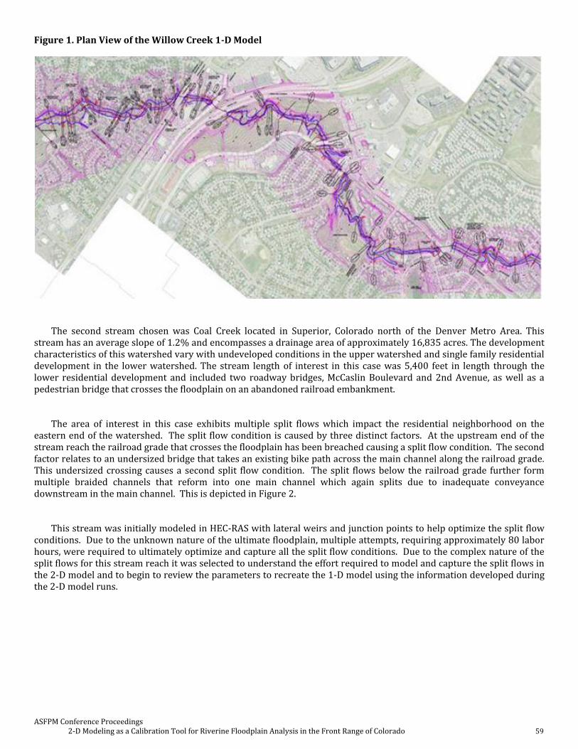
ASFPM Conference Proceedings 2-D Modeling as a Calibration Tool for Riverine Floodplain Analysis in the Front Range of Colorado 59

Figure 1. Plan View of the Willow Creek 1-D Model

The second stream chosen was Coal Creek located in Superior, Colorado north of the Denver Metro Area. This stream has an average slope of 1.2% and encompasses a drainage area of approximately 16,835 acres. The development characteristics of this watershed vary with undeveloped conditions in the upper watershed and single family residential development in the lower watershed. The stream length of interest in this case was 5,400 feet in length through the lower residential development and included two roadway bridges, McCaslin Boulevard and 2nd Avenue, as well as a pedestrian bridge that crosses the floodplain on an abandoned railroad embankment.

The area of interest in this case exhibits multiple split flows which impact the residential neighborhood on the eastern end of the watershed. The split flow condition is caused by three distinct factors. At the upstream end of the stream reach the railroad grade that crosses the floodplain has been breached causing a split flow condition. The second factor relates to an undersized bridge that takes an existing bike path across the main channel along the railroad grade. This undersized crossing causes a second split flow condition. The split flows below the railroad grade further form multiple braided channels that reform into one main channel which again splits due to inadequate conveyance downstream in the main channel. This is depicted in Figure 2.

This stream was initially modeled in HEC-RAS with lateral weirs and junction points to help optimize the split flow conditions. Due to the unknown nature of the ultimate floodplain, multiple attempts, requiring approximately 80 labor hours, were required to ultimately optimize and capture all the split flow conditions. Due to the complex nature of the split flows for this stream reach it was selected to understand the effort required to model and capture the split flows in the 2-D model and to begin to review the parameters to recreate the 1-D model using the information developed during the 2-D model runs.

ASFPM Conference Proceedings 2-D Modeling as a Calibration Tool for Riverine Floodplain Analysis in the Front Range of Colorado 60

Figure 2. Plan View of the Coal Creek 1-D Model

Figure 3. Plan View of the Westfield 1-D Model

The third case study selected was the Westfield Tributary to East Plum Creek in Castle Rock, Colorado. This stream is located south of the Denver Metro Area. This stream is a much smaller watershed than the previous two watersheds and encompasses approximately 441 acres and has an average slope of 3.5%. The existing land use within the basin is largely undeveloped with a few large acreage homes. The model included 3 hydraulic structures including a railroad crossing, frontage road crossing and the Interstate 25 crossing.

ASFPM Conference Proceedings 2-D Modeling as a Calibration Tool for Riverine Floodplain Analysis in the Front Range of Colorado 61

This stream was unique in that the outfall to East Plum Creek was not well defined. I-25, on the eastern edge of Figure 3 forms a physical barrier between East Plum Creek and the outfall of the Westfield Tributary. In developing the 1-D model assumptions were made as to where the main flow paths existed. Based on interviews with Town officials and local residents it was assumed that two main flow paths diverged and paralleled I-25 to an outfall culvert to the north of the channel and to an outfall culvert located south of the channel. There was evidence from the interviews that a third flow split occurred to the east over I-25, however it was assumed when developing the 1-D HEC-RAS model that this flow path was likely volume limited and would have a minimal floodplain and impact to I-25.

Development of 2-D Models

All of the 2-D models utilized similar development techniques. In all cases the underlying terrain data was 2-foot accuracy contours. These were converted into digital elevation maps in ArcView GIS and imported into the 2-D model to create the bathymetric data. The National Landuse Dataset raster produced by the U.S. Geological Survey (USGS, 2006) was used to populate the Manning's N value for the hydraulic computations. Land use was converted from the defined land use in the national dataset by utilizing the values in Table 1 below.

TABLE 1: Manning's N Values for selected land use covers.

Land Use or Cover Manning's N Value

Water 0.011

Concrete or Asphalt 0.020

Industrial 0.100

Commercial (Includes parking lots , vegetation and cars) 0.130

Residential Area (Includes structures, fences, cars and vegetation 0.200

Lawns, parks, open space with sparse trees and shrubs 0.090

Dense Brush, Trees, Natural Areas 0.110

Notes:

Finally, flow hydrographs previously developed were input to the 2-D grid in locations that replicated the tributary flow to the mainstem of interest. Flow rates in all cases were developed utilizing the Urban Drainage and Flood Control Districts (UDFCD) Colorado Urban Hydrograph Procedure (CUHP) computer program for sub-basin flow. These flows were then routed utilizing the Environmental Protection Agency's (EPA) Storm Water Management Model (SWMM) EPA-SWMM version 5. Table 2 below includes the major 2-D domain characteristics for each case study

TABLE 2

Case Study Grid Cell

Size (ft)

Total

number of

Grid Cells

Number of

Hydraulic

Structures

Number of

inflow

Hydrographs

Model run

time (hrs)

Model

Development

Time (hrs)

Willow Creek 14 168,801 10 31 96 160

Coal Creek 14 42,706 0 1 7 4

Westfield Tributary 14 134,771 3 6 3 4

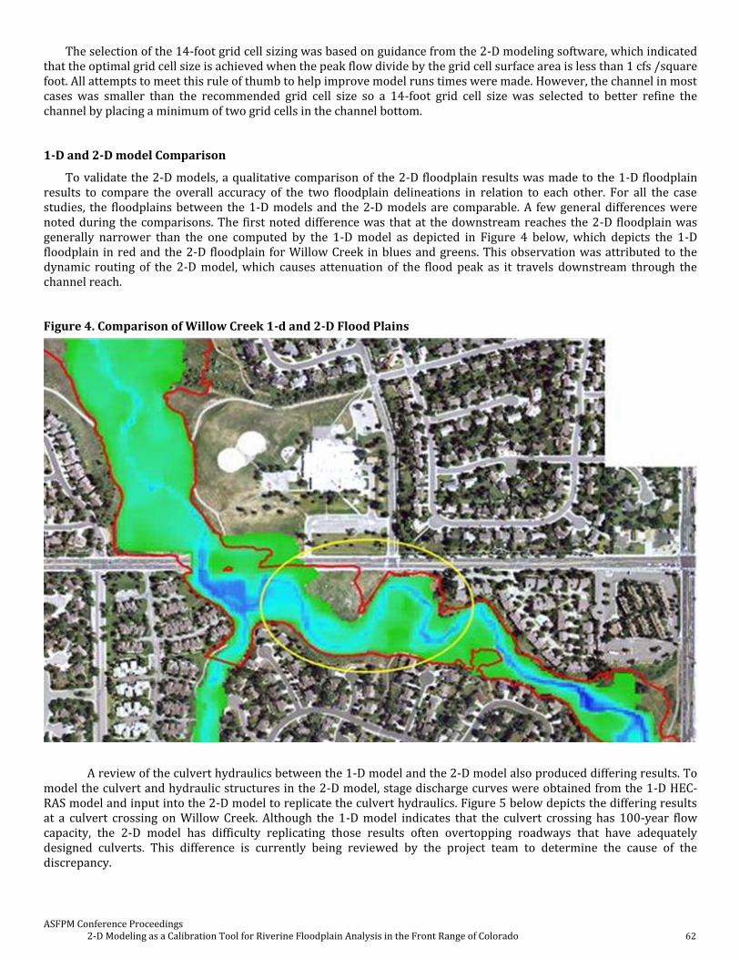
ASFPM Conference Proceedings 2-D Modeling as a Calibration Tool for Riverine Floodplain Analysis in the Front Range of Colorado 62

The selection of the 14-foot grid cell sizing was based on guidance from the 2-D modeling software, which indicated that the optimal grid cell size is achieved when the peak flow divide by the grid cell surface area is less than 1 cfs /square foot. All attempts to meet this rule of thumb to help improve model runs times were made. However, the channel in most cases was smaller than the recommended grid cell size so a 14-foot grid cell size was selected to better refine the channel by placing a minimum of two grid cells in the channel bottom.

1-D and 2-D model Comparison

To validate the 2-D models, a qualitative comparison of the 2-D floodplain results was made to the 1-D floodplain results to compare the overall accuracy of the two floodplain delineations in relation to each other. For all the case studies, the floodplains between the 1-D models and the 2-D models are comparable. A few general differences were noted during the comparisons. The first noted difference was that at the downstream reaches the 2-D floodplain was generally narrower than the one computed by the 1-D model as depicted in Figure 4 below, which depicts the 1-D floodplain in red and the 2-D floodplain for Willow Creek in blues and greens. This observation was attributed to the dynamic routing of the 2-D model, which causes attenuation of the flood peak as it travels downstream through the channel reach.

Figure 4. Comparison of Willow Creek 1-d and 2-D Flood Plains

A review of the culvert hydraulics between the 1-D model and the 2-D model also produced differing results. To model the culvert and hydraulic structures in the 2-D model, stage discharge curves were obtained from the 1-D HEC-RAS model and input into the 2-D model to replicate the culvert hydraulics. Figure 5 below depicts the differing results at a culvert crossing on Willow Creek. Although the 1-D model indicates that the culvert crossing has 100-year flow capacity, the 2-D model has difficulty replicating those results often overtopping roadways that have adequately designed culverts. This difference is currently being reviewed by the project team to determine the cause of the discrepancy.

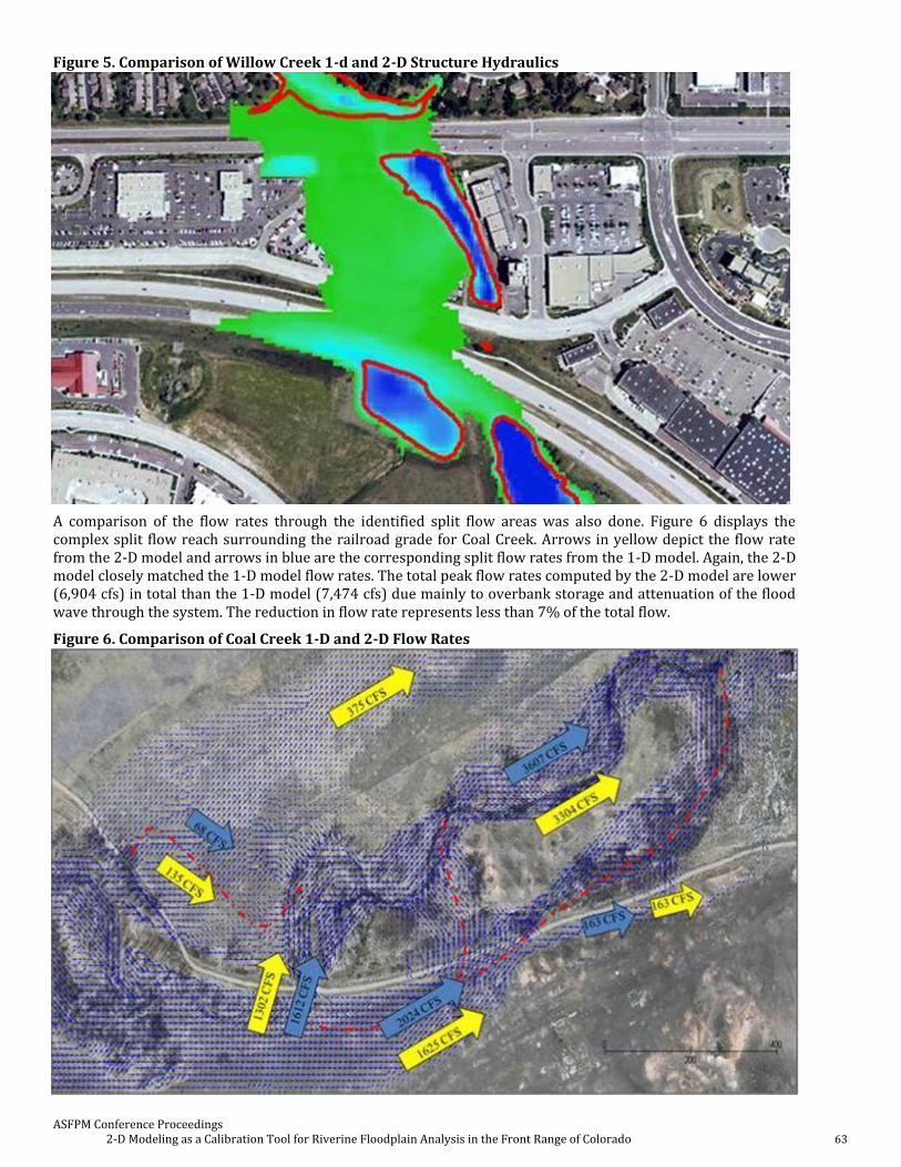
ASFPM Conference Proceedings 2-D Modeling as a Calibration Tool for Riverine Floodplain Analysis in the Front Range of Colorado 63

Figure 5. Comparison of Willow Creek 1-d and 2-D Structure Hydraulics

A comparison of the flow rates through the identified split flow areas was also done. Figure 6 displays the complex split flow reach surrounding the railroad grade for Coal Creek. Arrows in yellow depict the flow rate from the 2-D model and arrows in blue are the corresponding split flow rates from the 1-D model. Again, the 2-D model closely matched the 1-D model flow rates. The total peak flow rates computed by the 2-D model are lower (6,904 cfs) in total than the 1-D model (7,474 cfs) due mainly to overbank storage and attenuation of the flood wave through the system. The reduction in flow rate represents less than 7% of the total flow.

Figure 6. Comparison of Coal Creek 1-D and 2-D Flow Rates

ASFPM Conference Proceedings 2-D Modeling as a Calibration Tool for Riverine Floodplain Analysis in the Front Range of Colorado 64

How to go from a 2-D model to a 1-D model: General Guidance and Observations

Based on the analysis and the experience of the project team in developing the data for this paper, two general guidelines and observations were made that form the basis for model selection and floodplain analysis using either 1-D models or 2-D models.

1. Channelized river systems are better represented by 1-D Models.

Based on the experience modeling the Willow Creek floodplain in both a 1-D and 2-D model, it was found that the model set up time as and the debugging of the 2-D model were similar in nature to setting up a 1-D model, approximately 2-weeks. Based on this there was not a significant efficiency gain or timesavings that improved the delineation or understanding of the floodplain characteristics by utilizing the 2-D model.

2. River systems with complex split flows, unknown flow paths, and urban areas are better modeled in 2-D simulations and then moved to 1-D models for regulatory implementation.

The experience with Coal Creek and Westfield Tributaries realized significant efficacy improvements and timesavings as well as a better understanding of the split flow paths and floodplain behavior with the 2-D models. It was also found that the results of the 2-D modeling could be used to validate and build a 1-D model that would create similar results to the 2-D model.

Conclusions

1-D models will be the regulatory legacy for many years to come as the majority of floodplains throughout the U.S. have 1-D models for the basis of the regulation. There is a recent push to provide better more accurate floodplain data to better understand both the risk and hazard of floodplains areas. Improvements in technology, computing power and terrain data have led to the widespread acceptance of 2-D models. This paper has demonstrated the usefulness of 2-D models in improving both efficiency and accuracy of complex floodplains by helping to eliminate the guesswork and assumptions made to complete 1-D models and by helping reduce the model development time for complex systems.

However, the unsteady dynamic nature of 2-D models provides difficulties for jurisdictions in providing effective regulation of floodplains developed using 2-D models. Current regulations through The National Flood Insurance Policy were developed to reflect the floodplain data produced by 1-D models. By utilizing 2-D models, by conserving and computing flow volume, attenuating flow rates, and computing water surface elevations at each discretized grid cell cause difficulties with existing regulations that regulate to peak flow rates, Base Flood Elevations and floodways. By utilizing, the power of 2-D models to better define and create 1-D models, regulators and jurisdictions can take advantage of the improved efficiency and accuracy of 2-D models while providing a regulatory 1-D model that works with current regulations.