2009 Bioenergy

Report

Assessment of inter-linkages between bioenergy development and water availability ENV.D.2/SER/2008/0003r

July 2009

Ecologic – Institute for International and European Environmental Policy Berlin/Vienna

In co-operation with

The Authors:

Thomas Dworak (Ecologic Institute-Vienna) Berien Elbersen, Kees van Diepen, Igor Staritsky, Daniel van Kraalingen, Ivan Suppit (Alterra) Maria Berglund, Timo Kaphengst, Cornelius Laaser (Ecologic Institute-Berlin) Maria Ribeiro (Ecologic Institute-Vienna)

Ecologic, Institute for International and European Environmental Policy Auhofstrasse 4/7, 1130 Vienna, Austria, Tel: +43-664 73 59 2278 | Fax: +43-1-877 64 30 E-Mail: [email protected], www.ecologic.eu

-1-

mailto:[email protected]

-2-

TABLE OF CONTENT

DRAFT REPORT ........................................................................................................................................................................................1

ENV.D.2/SER/2008/0003R .......................................................................................................................................................................1

JULY 2009................................................................................................................................................................................................1

ECOLOGIC – INSTITUTE FOR INTERNATIONAL AND EUROPEAN ENVIRONMENTAL POLICY BERLIN/VIENNA ...............................................1

ACKNOWLEDGMENTS..............................................................................................................................................................................4

1 INTRODUCTION AND POLICY CONTEXT............................................................................................................................................5

1.1 AGRICULTURAL BIOENERGY PRODUCTION: EU POLICIES AND ENVIRONMENTAL ASPECTS......................................................................................... 5 1.2 OBJECTIVES OF THE STUDY......................................................................................................................................................................... 7

2 MAIN DEFINITIONS USED ................................................................................................................................................................8

3 WATER USE IN THE AGRICULTURAL BIOENERGY PATHWAYS ..........................................................................................................10

4 APPROACH TAKEN.........................................................................................................................................................................13

4.1 OVERALL APPROACH............................................................................................................................................................................... 13 4.2 ESTIMATING PRESENT IRRIGATION SHARES AND IRRIGATION WATER REQUIREMENTS FOR BIOENERGY CROPPING........................................................ 14 4.3 PREDICTING FUTURE CULTIVATION AND IRRIGATION PATTERNS AND WATER REQUIREMENTS FOR BIOENERGY CROPPING ............................................. 15

5 CURRENT ENERGY CROPS DISTRIBUTION IN THE EU.......................................................................................................................16

5.1 CURRENT WATER USE OF BIOENERGY CROPPING........................................................................................................................................... 17

6 IMPACTS OF FUTURE BIOENERGY DEVELOPMENTS ON IRRIGATION WATER DEMAND....................................................................20

6.1 THE THREE STORYLINES/SCENARIOS IN A NUTSHELL....................................................................................................................................... 20 6.2 MAIN DRIVERS INFLUENCING THE FUTURE OF BIOENERGY CROPPING WITHIN THE CURRENT POLICY FRAMEWORK ...................................................... 20 6.3 THE THREE STORYLINES IN DETAIL.............................................................................................................................................................. 25

6.3.1 Storyline 1: Business as Usual....................................................................................................................................................... 25 6.3.2 Storyline 2: Increased irrigation water demand........................................................................................................................... 26 6.3.3 Storyline 3: Water saving scenario – implications for the bioenergy targets............................................................................... 28 6.3.4 Implementation of the storyline specifications into calculation of irrigation requirements and biomass and energy yields ...... 28

6.4 UNCERTAINTIES IN THE STORYLINE DEVELOPMENT ........................................................................................................................................ 30 6.5 SCENARIO RESULTS................................................................................................................................................................................. 30

7 BIOENERGY IN THE CONTEXT OF CURRENT RIVER BASIN PLANNING...............................................................................................41

8 CONCLUSION AND RECOMMENDATIONS.......................................................................................................................................43

9 BIBLIOGRAPHY ..............................................................................................................................................................................45

ANNEX 1: DETAILED DESCRIPTION OF THE METHODS USED TO ESTIMATE WATER REQUIREMENTS AND YIELD LEVEL FOR BIOMASS CROPPING IN THE PRESENT AND FUTURE SITUATION.............................................................................................................................49

1. DEFINING THE STATE OF THE ART IN CROP GROWTH MODELLING AND CROP WATER REQUIREMENTS............................................................................ 49 2. FURTHER TECHNICAL DETAILS ON THE MODEL APPROACH TO ESTIMATING THE CURRENT WATER NEEDS OF BIOENERGY CROPS .......................................... 53 3. MODELLING OF WATER REQUIREMENTS OF PERENNIAL GRASSES FOR ESTIMATING FUTURE BIOENERGY IRRIGATION WATER REQUIREMENTS ........................ 55 4. IMPLEMENTATION OF 3 SCENARIO/STORYLINE SPECIFICATIONS INTO QUALITATIVE ESTIMATES OF IRRIGATION WATER USE, BIOMASS AND ENERGY YIELD LEVELS

PER RBD........................................................................................................................................................................................................... 80

ANNEX 2: PRESENT AREA OF ENERGY CROPS IN THE EU AND SOURCES USED .........................................................................................87

1. PRESENT AREA OF ENERGY CROPS IN THE EU (2006/2007)............................................................................................................................... 87

-3-

2. SOURCES .................................................................................................................................................................................................. 90

ANNEX 3: EUROPEAN RIVER BASINS AFFECTED BY WATER SCARCITY TODAY..........................................................................................97

ANNEX 4: CROP WATER REQUIREMENTS ............................................................................................................................................. 101

ANNEX 5: SUMMARY OF PRESENT SHARE OF BIOENERGY CROPS IN TOTAL CROPPING AREA AND IRRIGATION WATER USE.................. 102

ANNEX 6: CAPSIM ANIMLIB SCENARIO................................................................................................................................................. 105

ANNEX 7: STORYLINE CALCULATION RESULTS PER RBD ........................................................................................................................ 107

ANNEX 8: THE LINK BETWEEN WATER QUALITY AND QUANTITY........................................................................................................... 138

-4-

Acknowledgments

This report would not have been possible without the help of:

Martina Flörke and her team from the University of Kassel, who provided us with relevant data from their „WATERGAP“ model.

Gunter Wriedt, Marijn van der Velde, Alberto Aloe, Fayçal Bouraoui (JRC) who provided us information on the water requirements for irrigation in the European Union.

Ayis I. Iacovides (I.A.C.O), Josefina Maestru (Ministry of Environment of Spain), Nikzentaitis Vaidotas (SE Energy Agency), Panoutsou, Calliope (Imperial College, UK), Sven-Olov Ericson (Ministry of Enterprise, Energy and.

Communication, Sweden), Reskola Veli-Pekka (Ministry of Agriculture and Forestry, Finland) and Paweł Rutkowski (Warsaw University) who supported us with obtaining relevant information on the status of bioenergy cropping in the

various Member States.

-5-

1 Introduction and policy context In recent years, a growing concern has been expressed throughout the EU regarding drought events and water scarcity problems. Generally speaking, water scarcity is considered to occur when “there are insufficient water resources to satisfy long-term average requirements. Water scarcity refers to long-term water imbalances, combining low water availability with a level of water demand exceeding the supply capacity of the natural system” (European Commission, 2006a).

1.1 Agricultural bioenergy production: EU policies and environmental aspects The number of Member States (MS) that experience seasonal or long term droughts has increased over the years. In recognition of the acuteness of the water scarcity and drought challenges in Europe, the Commission undertook in 2006 and early 2007 an in-depth assessment of the situation at EU level. Furthermore, in July 2007 the Commission adopted a Communication on Water Scarcity and Droughts1, which identified an initial set of policy options to be taken at European, national and regional levels to address water scarcity within the Union. This set of proposed policies aims to move the EU towards a water-efficient and water-saving economy. One important factor in this context is future land use, which is crucial for mitigating water stress in the long run.

In parallel to these developments, bioenergy is becoming a more important energy source in order to reduce reliance on fossil sources and foreign imports. Bioenergies are also discussed as an important option to reduce greenhouse gas emissions, although there are also several concerns about this benefit2. On 17th of December 2008, the European Parliament accepted the Directive proposed by the European Commission on the promotion of the use of energy from renewable sources (European Parliament and of the Council, 2009). It sets out:

• a binding 20% target for the overall share of renewable energy by 2020 – the effort to be shared in an appropriate manner among MS; and

• a binding target for the share of renewable energy in the transport sector of 5% by 2015 and 10% by 2020.

• The legislation also includes standard criteria renewable energy production has to comply with in order to count towards the binding target.

• To reduce the risk of a negative GHG emissions, the Directive provides rules for calculating the greenhouse gas impact of biofuels, other bioliquids and their fossil fuel counterparts.

Three sectors are most relevant for renewable energy: electricity, heating and cooling and transport. It is up to the MS to decide on the mix of contributions from these sectors to reach their national targets and to choose the means that best suits their national circumstances. MS are also given the option to achieve their targets by supporting the development of renewable energy in other MS and third countries. Each MS shall adopt a national action plan setting out targets for the share of energy in 2020 and adequate measures to be taken to achieve these targets, including national policies to develop existing biomass resources and mobilise new biomass resources for different uses. The plans have to be forwarded to the Commission by 31 March 2010 at the latest.

1 See http://ec.europa.eu/environment/water/quantity/scarcity_en.htm 2 When all emissions are included using a life cycle analysis, the GHG mitigation benefits of bioenergies are quite variable and not always as good as has been claimed. Related emissions include emissions produced during the production and application of fertilizers, emission related to the transport of feedstocks and conversion and when carbon stocks in the soil and the covering vegetation are depleted as a result of land use change. However significant uncertainties surround the lifecycle GHG savings of bioenergies, in part because direct and indirect land uses effects are not adequately covered in current LCA. A review of around 60 recent life cycle analysis published confirmed that there are wide ranges of GHG balances, not always leading to positive results. For further details see: International Energy Agency (2008).

-6-

Feedstocks from agriculture will play an important role since it can be used in all three sectors and will be the main source for bioenergy production as long as second generation conversion techniques based on ligno-cellulosic material are not economical.

Therefore, the targets set by the EU for increasing biomass production necessitate substantial growth in agriculture production, which already led to a debate concerning potential benefits to the environment as well as possible conflicts with objectives of other EU policies, such as the Water Framework Directive (WFD)(European Parliament and Council, 2000). Intensive agriculture is a key driver preventing waters from achieving good status as required by the WFD (Kampa et al., 2009). However, the WFD itself sets outs provisions that allow achieving lower water status in the case of new modifications or as a result of new sustainable human development activities (see Box 1).

Box 1: Exemptions under the WFD

According to Art. 4.7 WFD Member States will not be in breach of this Directive when:

• failure to achieve good groundwater status, good ecological status or, where relevant, good ecological potential or to prevent deterioration in the status of a body of surface water or groundwater is the result of new modifications to the physical characteristics of a surface water body or alterations to the level of bodies of groundwater, or

• failure to prevent deterioration from high status to good status of a body of surface water is the result of new sustainable human development activities.

Growing bioenergy crops and the related construction of new reservoirs for irrigation might fall under these provisions, as large-scale bioenergy cropping may significantly increase land use intensity in several European regions. This may also cause, in particular, negative impacts on water quantity and quality as both issues are often influencing each other (see Annex 8).

Being aware of the environmental risks that can occur from certain farming practices and to reduce the risks of uncontrolled intensification, the EU`s Common Agricultural Policy (CAP) provides several safe guard mechanisms under its cross compliance scheme (European Council, 2003). Since 2005 all farmers receiving direct payments3 must respect Cross Compliance standards in two ways:

• First, they must respect the Statutory Management Requirements set-up in accordance with 19 EU Directives and Regulations4. The standards relate to the protection of the environment; public, animal and plant health; and animal welfare. With regard to water management, the most important Directives covered by Cross Compliance are the Groundwater Directive (80/68/EEC) and the Nitrate Directive (91/676/EEC) and to some extent the Sewage Sludge Directive (Directive 86/278/EEC), which will also be part of the River Basin (RB) management plans under the WFD.

• Second, all agricultural land for which farmers claim payment should be kept in Good Agricultural and Environmental Condition (GAEC). In general, GAEC’s focus is on the protection of soil and its positive side-effects on the reduction of diffuse pollution. It is up to the individual MS to define minimum GAEC requirements, which may differ depending on local conditions.

3 The main aim of the direct payment is to guarantee farmers more stable incomes. Farmers can decide what to produce in the knowledge that they will receive the same amount of aid, allowing them to adjust production to suit demand. 4 The Directives relevant to water protection are the Groundwater Directive (Art. 3), the Sewage Sludge Directive (Art. 3), the Nitrates Directive (Art. 4 and 5), the Conservation of Wild Birds (Art. 3, 4 (1), (2), (4), 5, 7 and 8), and the Conservation of natural habitats, wild flora and fauna (Art. 6, 13, 15, and 22(b)).

-7-

Furthermore, on 20 November 2008 the EU Agriculture Council reached a political agreement on the Health Check of the Common Policy (European Council, 2009). The “Health Check” agreement includes the addition of new standards related to water into the Good Agricultural and Environmental Condition (GAEC) of cross-compliance. Firstly, it includes new cross compliance elements in the Good Agricultural and Environmental Condition (GAEC) part: the new issue on the protection and management of water is designed to protect water against pollution and run-off and manage the use of water. This will involve the obligation of MS to require the establishment of buffer strips along water courses and to ensure compliance with authorisation procedures in cases where the use of water for irrigation is subject to authorisation. The start date for the irrigation GAEC is 1/1/2010; the buffer strip GAEC may start then as well but MS are only obliged to introduce it by 1/1/2012.

Further, under the Health Check the former requirement for arable farmers receiving direct payments to leave 10% of their land under set-aside is abolished. This abolishment was approved to allow farmers to maximise their production potential. Also, the energy crop premium (a premium of 31 € per hectare in 2007) has been abolished.

Within this policy framework future bioenergy production will develop. No clear storyline of these developments is available and the development will strongly depend on how MS implement the WFD and which measures will be taken to fulfil the obligations of the Renewable Energy Directive.

1.2 Objectives of the study It is in this context that the European Commission has tendered a study with following specific objectives:

• Analyse the different water needs and distribution of bioenergy crops grown or potentially grown in the next decades in the EU;

• Develop three scenarios focusing on future bioenergy developments and related land use until 2020;

• Assess the impacts of an increased bioenergy cropping on the River Basin level on future water availability for 2020 according to the 3 scenarios; and

• Support the Commission in linking water scarcity issues to agricultural policies.

-8-

2 Main definitions used

Water saving is one measure to avoid water scarcity and to improve aquatic ecosystems in the European Union (European Commission, 2006b). To have a common understanding of the terms related to water saving and bioenergy cropping some terms are clarified:

• Water demand/use is the total volume of water needed to satisfy the different water services5, including volumes ‘lost’ during transport, for example leaks from pipes and evaporation. In this study only the irrigation water demand is addressed.

• Water consumption relates to the amount of water abstracted which is no longer available for use because it has evaporated, transpired, been incorporated into products and crops, consumed by humans or livestock, ejected directly into sea, or otherwise removed from freshwater resources.

• Bioenergy from agriculture can in theory be produced from all types of plants (crops, trees, grassland cuttings and other plant residues) and from animal by-products/wastes. These agricultural biomass sources can be converted into electricity, heat and biofuels. In practice only a few sources from agriculture are used in the EU for conversion into bioenergy because of (current) use of these resources for other purposes, and/or technical and economic barriers.

• Biofuels for transport are currently in the EU (in 1st generation technologies) mainly converted from:

o oil seeds (rape, sunflower) or animal fats through transesterification into biodiesel and

o starch crops (maize, wheat, rye, potatoes) and sugar crops (sugar beet) through fermentation into bioethanol.

• For biogas production, mainly starch crops (maize and cereals) and/or animal manure are converted into gas through anaerobic digestion. Other feedstocks include harvest residues (straw), energy grasses (e.g. Miscanthus, giant reed) and grassland cuttings.

• First generation biofuels are made from sugar, starch, vegetable oil, or animal fats for which the conversion process is considered to be based on established (including commercial) technologies.

• Second generation biofuels are carbon-based fuels whose conversion is still based on several innovative process which are still under development and not yet commercial. They are produced from lignocellulosic biomass such as crop and forest residues, straw and or woody biomass crops (e.g. perennial grasses such Miscanthus, switchgrass, reed canary grass etc. and short rotation coppice trees such as willow, poplar).

• Crop water requirements: The transpiration of arable crops is one of the basic components of the water balance. To determine the impacts of bioenergy cropping on the water balance in the area of interest it is required to estimate the crop mix, their rotation and the type of irrigation. For bioenergy cropping currently four categories of plants can be identified:

o Classical crops: Today’s agricultural biomass production for bioenergy is mainly derived from rotational arable food crops such as maize, wheat, barley, sugar beet, potatoes and oil seeds (rape, sunflower). The production requirements of these crops when used for bioenergy are in principle not different from when they are used for feed and food purposes. It is expected however that this will

5 In this study water service refers to water supply and waste water removal.

-9-

change in the future as new varieties and species (including Genetic Modified Organisms) will be introduced more adapted to the requirements of a more efficient conversion process.

o Novel crops: Several research projects have started to investigate new or non-common crops which can be used as feedstock for bioenergy. These plants should provide considerable opportunities for increasing bioenergy production in the future, given their specific characteristics such as the ability to produce high yield under relatively poor (low input) situations. This also includes crops that may still deliver relatively high yields per hectare on poor soils (e.g. ‘waste’ lands or abandoned lands) or with no additional irrigation requirements. Further development work is needed, however, to establish these new crops for widespread cultivation (Joint Research Centre of the EU, European Environmental Agency, 2006) in different bio-climatic circumstances. Examples of such crops which are already under widespread investigation in the EU are Jerusalem artichoke (Helianthus tuberosus), Sweet sorghum (Sorghum bicolor), Cynara (Cynara cardunculus) or Castor bean (Ricinus communis) etc.

o Perennial biomass crops include woody species of short rotation coppices (SRC) (e.g. poplar and willow) and perennial energy grasses (e.g. Switchgrass, Miscanthus, Reed canary grass, Giant reed). Both SRC and perennial biomass grasses have a multi-annual lifecycle that can extend from 10 to 20 years and they have deep rooting systems. Because of this they are expected to have lower environmental impacts than most annual plants have (European Environment Agency, 2007) since their mechanisation and input requirements are generally lower per unit of production. The high hemi-cellulose and cellulose content of these woody crops potentially result in favourable net energy conversion ratios.

o Perennial grasses (Miscanthus, Reed canary grass, Giant reed, Switch grass) and Short Rotation Coppices (SRC) (e.g. willow and poplar) are recognised to provide a considerable opportunity to more sustainable bioenergy production but their use is currently severely limited. The technology for an efficient conversion of these crops, 2nd generation technology, is not expected to become commercially available before 2020. The introduction of these crops can therefore not be expected to take off as from 5 to 10 years from now. Furthermore, with the wide-spread commercial introduction of 2nd generation conversion technologies it is also expected that the need for land for biomass cropping will decrease as the use of ligno-cellulosic by- and waste products will increase.

-10-

3 Water use in the agricultural bioenergy pathways

Water use in bioenergy cropping is most relevant during crop production and conversion. At the crop production stage, local and regional considerations play a considerable role in water consumption and water use efficiency (WUE)6 as well as whether the feedstock is irrigated or not. Water use efficiency varies greatly among crop types: genrally C4 crops have higher WUE and productivity than C3 crops; perennial crops generally consume more water (if available) than annual crops but have higher yields (also per unit of water). Furthermore, water consumption and WUE depend on climate conditions, growing period and agronomic practice and also availability of water. Perennials also have a higher chance to deplete water resources because of their deeper rooting system, so in spite of their generally more efficient water use they can still cause unsustainable water use.

The wide range in WUE per crop is illustrated by the underneath estimates (in kg DM ha-1 mm-1 evapotranspiration) based on Berndes, 2002:

• Rapeseed: around 9-12 kg DM ha-1 mm-1;

• Sugarcane 17-33 kg DM ha-1 mm-1;

• Sugar beet 9-24 kg DM ha-1 mm-1;

• Corn 7-21 kg DM ha-1 mm-1;

• Wheat 6-36 kg DM ha-1 mm-1;

• lignocellulosic crops it can range between 9-95 kg DM ha-1 mm-1.

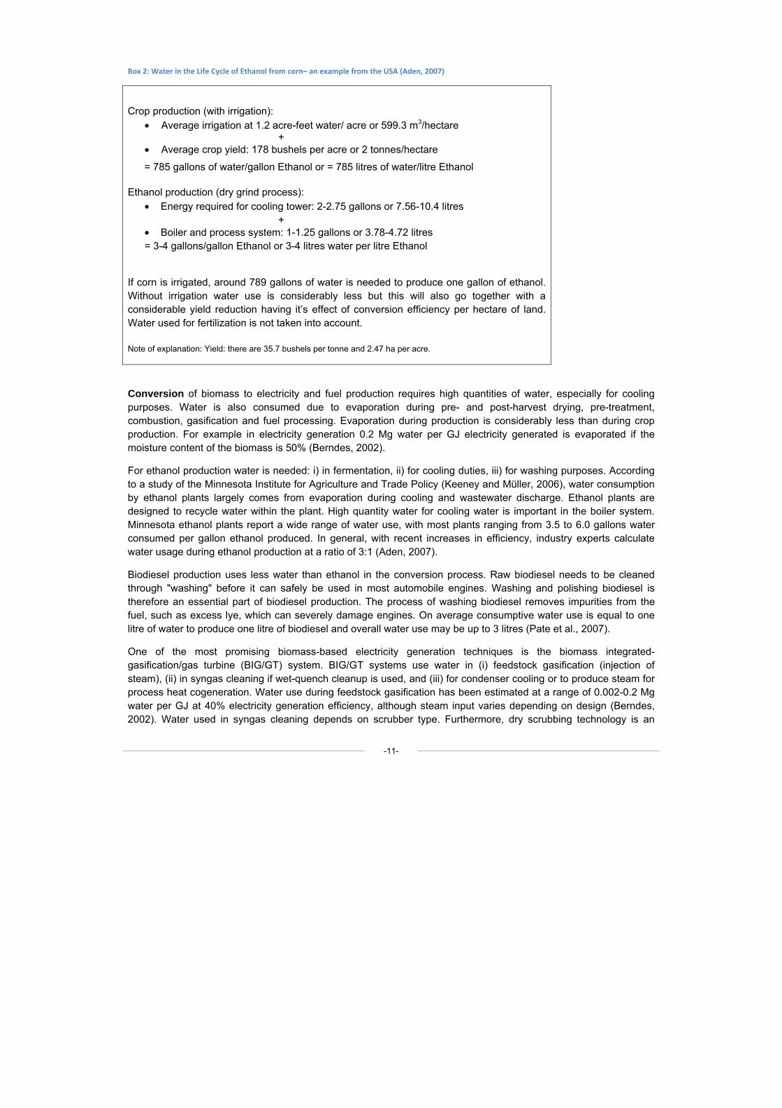
Water consumption is most significant for irrigated crops. At the moment bioenergy feedstocks in Europe are mostly rain fed; however, with increasing water scarcity as well as uncertainty regarding future climate conditions, the irrigated area for these crops will most likely increase. Data regarding total irrigation area and water consumption shre for bioenergy cropping are practically absent (see also Chapter 5 and Annex 2). According to a 2003 United States Department of Agriculture Farm survey, irrigated corn/maize requires around 785 gallons of water to produce one gallon of ethanol (see Box below)

6 Water Use Efficiency (WUE) is the amount of dry aboveground biomass produced per unit of evapotranspired water.

-11-

Box 2: Water in the Life Cycle of Ethanol from corn– an example from the USA (Aden, 2007)

Crop production (with irrigation): • Average irrigation at 1.2 acre-feet water/ acre or 599.3 m3/hectare

+ • Average crop yield: 178 bushels per acre or 2 tonnes/hectare

= 785 gallons of water/gallon Ethanol or = 785 litres of water/litre Ethanol Ethanol production (dry grind process):

• Energy required for cooling tower: 2-2.75 gallons or 7.56-10.4 litres +

• Boiler and process system: 1-1.25 gallons or 3.78-4.72 litres = 3-4 gallons/gallon Ethanol or 3-4 litres water per litre Ethanol

If corn is irrigated, around 789 gallons of water is needed to produce one gallon of ethanol. Without irrigation water use is considerably less but this will also go together with a considerable yield reduction having it’s effect of conversion efficiency per hectare of land. Water used for fertilization is not taken into account. Note of explanation: Yield: there are 35.7 bushels per tonne and 2.47 ha per acre.

Conversion of biomass to electricity and fuel production requires high quantities of water, especially for cooling purposes. Water is also consumed due to evaporation during pre- and post-harvest drying, pre-treatment, combustion, gasification and fuel processing. Evaporation during production is considerably less than during crop production. For example in electricity generation 0.2 Mg water per GJ electricity generated is evaporated if the moisture content of the biomass is 50% (Berndes, 2002).

For ethanol production water is needed: i) in fermentation, ii) for cooling duties, iii) for washing purposes. According to a study of the Minnesota Institute for Agriculture and Trade Policy (Keeney and Müller, 2006), water consumption by ethanol plants largely comes from evaporation during cooling and wastewater discharge. Ethanol plants are designed to recycle water within the plant. High quantity water for cooling water is important in the boiler system. Minnesota ethanol plants report a wide range of water use, with most plants ranging from 3.5 to 6.0 gallons water consumed per gallon ethanol produced. In general, with recent increases in efficiency, industry experts calculate water usage during ethanol production at a ratio of 3:1 (Aden, 2007).

Biodiesel production uses less water than ethanol in the conversion process. Raw biodiesel needs to be cleaned through "washing" before it can safely be used in most automobile engines. Washing and polishing biodiesel is therefore an essential part of biodiesel production. The process of washing biodiesel removes impurities from the fuel, such as excess lye, which can severely damage engines. On average consumptive water use is equal to one litre of water to produce one litre of biodiesel and overall water use may be up to 3 litres (Pate et al., 2007).

One of the most promising biomass-based electricity generation techniques is the biomass integrated-gasification/gas turbine (BIG/GT) system. BIG/GT systems use water in (i) feedstock gasification (injection of steam), (ii) in syngas cleaning if wet-quench cleanup is used, and (iii) for condenser cooling or to produce steam for process heat cogeneration. Water use during feedstock gasification has been estimated at a range of 0.002-0.2 Mg water per GJ at 40% electricity generation efficiency, although steam input varies depending on design (Berndes, 2002). Water used in syngas cleaning depends on scrubber type. Furthermore, dry scrubbing technology is an

-12-

option and can reduce water use. Much of the water used is recycled through wastewater treatment and does not add significant to consumptive water totals.

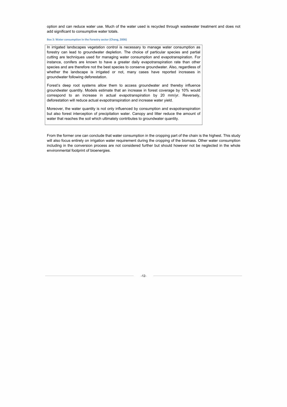
Box 3: Water consumption in the Forestry sector (Chang, 2006)

In irrigated landscapes vegetation control is necessary to manage water consumption as forestry can lead to groundwater depletion. The choice of particular species and partial cutting are techniques used for managing water consumption and evapotranspiration. For instance, conifers are known to have a greater daily evapotranspiration rate than other species and are therefore not the best species to conserve groundwater. Also, regardless of whether the landscape is irrigated or not, many cases have reported increases in groundwater following deforestation.

Forest’s deep root systems allow them to access groundwater and thereby influence groundwater quantity. Models estimate that an increase in forest coverage by 10% would correspond to an increase in actual evapotranspiration by 20 mm/yr. Reversely, deforestation will reduce actual evapotranspiration and increase water yield.

Moreover, the water quantity is not only influenced by consumption and evapotranspiration but also forest interception of precipitation water. Canopy and litter reduce the amount of water that reaches the soil which ultimately contributes to groundwater quantity.

From the former one can conclude that water consumption in the cropping part of the chain is the highest. This study will also focus entirely on irrigation water requirement during the cropping of the biomass. Other water consumption including in the conversion process are not considered further but should however not be neglected in the whole environmental footprint of bioenergies.

4 Approach taken

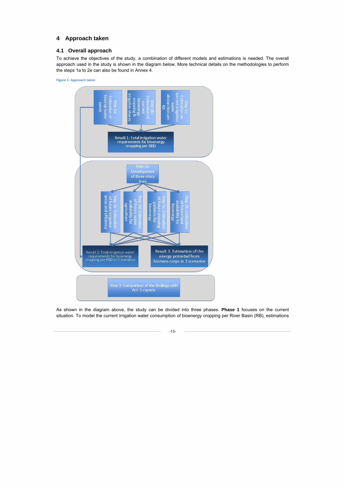
4.1 Overall approach To achieve the objectives of the study, a combination of different models and estimations is needed. The overall approach used in the study is shown in the diagram below. More technical details on the methodologies to perform the steps 1a to 2e can also be found in Annex 4.

Figure 1: Approach taken

As shown in the diagram above, the study can be divided into three phases. Phase 1 focuses on the current situation. To model the current irrigation water consumption of bioenergy cropping per River Basin (RB), estimations

-13-

-14-

were calculated for: i) crop water requirements per bioenergy crop; ii) the current bioenergy crops distribution and irrigation share in the EU-MS and iii) current water abstraction for irrigation per River Basins. Through the combination of these three elements, it is possible to estimate the total irrigation water requirements and share of total irrigation water consumption for current bioenergy cropping in each River Basin.

Under phase 2 three different storylines/scenarios were developed, drawing possible future developments of biomass cropping up to 2020. Based on these storylines, estimations were made about i) future land availability, ii) future cropping patterns and irrigation shares, iii) future water availability for the agricultural sector and iv) the development of future irrigation areas.

Finally, the results of phase 2 were compared with the Art. 5. Reports required by the WFD. In these reports (phase 3) MS should forecast future water consumption. These comparisons make it possible to judge the extent to which future bioenergy cropping is considered in each RB report.

4.2 Estimating present irrigation shares and irrigation water requirements for bioenergy cropping

Several steps were performed to calculate the relative irrigation water needs for different bioenergy crops.

Step 1: Estimation of the biomass cropping area and crop mix per region: To estimate the relative irrigation share it was necessary to first collect data per country on total bioenergy cropping area and types of bioenergy crops used. This information could be found through internet search and consultations with experts in different countries. An overview of the sources used is given in Annex 2 and a summary of the collected information is given in Table 1 in Chapter 5. It turned out that the information needed could generally be derived at national level, but that regional specific information was very difficult to be obtained, except for Spain and UK.

Step 2: Allocation of biomass crops to NUTS-2 regions: For the estimation of the irrigation water needs per crop and the further distribution of crops to River Basin Districts (RBD) it was necessary to further allocate crops first to NUTS-2 regions for countries at which this information was not made available at this level. To do this it was assumed that bioenergy crops are distributed regionally in the same way as conventional agricultural crops used for feed and food purposes. Data from Eurostat (Farm Structural Survey data, 2005) on the main crop shares per NUTS-2 were therefore used as a weighting factor to distribute the bioenergy crops over regions. The crops used as weighting were rape, sunflower, cereals (mix of wheat, barley), maize (corn and fodder maize) and sugarbeet.

Step 3: Estimation of irrigated area (share) of bioenergy crops: From the sources consulted it was not possible to obtain any hard information on the area of biomass crops under irrigation. The assumption was therefore made that all bioenergy crops are produced in the same way as conventional crops and are therefore assumed to be irrigated to the same extent as similar crops grown in the same region but then for food or feed purposes. The present irrigation share per crop per NUTS-2 region was then used as a weighting factor to apply to the total regional cropping area of the bioenergy crop. Figures on crop specific irrigation shares per NUTS-2 were obtained from the JRC database on water requirements for irrigation (Wriedt et al., 2008). This database contains statistical data on irrigation per crop obtained from Eurostat (FSS 2003) which have been allocated to a 10*10 km grid in a statistical and rule based procedure for the whole of Europe using different additional spatial information sources and local information on irrigation practices.

Step 4: Calculation of the irrigation water requirement per crop per region: The irrigation water requirement has been calculated as the total amount of water (in cm water layer per unit area) needed by a certain crop in addition to the rainfall for the realization of maximum potential yield. This maximum potential yield is defined as the maximum yield under prevailing weather conditions without any other growth constraints. In the absence of irrigation the maximum yield under rainfed conditions is determined by the amount of rainfall and its distribution over the growing season. This maximum water-limited yield is equal tot the potential yield in the case of sufficient rainfall, and is lower than the

-15-

potential yield in the case of drought. Both the potential and water-limited yield and the amount of water directly used by the crops for transpiration under potential conditions have been extracted from the data base of the Crop Growth Monitoring System (CGMS) of the MARS project of the Joint Research Centre.

Step 5: Once the per hectare irrigation water requirements were calculated in (step 4) these were multiplied by the total irrigated area every biomass crop was estimated to use (in step 3). This multiplication resulted in a total irrigation water requirements per NUTS-2 region. The final step was then to allocate the NUTS-2 irrigation water needs for bioenergy crops to the River Basin Districts (RBD) and to express them in relative shares in the total irrigation water needs per RBD. How this was done is further explained in Annex 1.

In Annex 1 further details are given given of the way the calculations of the irrigation water needs are made by the CGMS system and further details of all other steps described above. The Annex starts with an overview of the state of the art in crop growth and water use modelling and this is followed by the more technical details of how the CGMS system works and how the above described steps 2 to 5 were performed.

4.3 Predicting future cultivation and irrigation patterns and water requirements for bioenergy cropping

For the prediction of future water requirements of biomass cropping several steps were taken. Underneath the general brief characterisation of these steps is given and the more detailed and technical description of these steps is provided in Annex 2 (Section 3) and Chapter 6 where the three storylines according to which future bioenergy cropping and related irrigation water needs are described.

Step 1: Estimation is made of the future land and irrigation water availability per NUTS-2 region in three different storylines. In Chapter 6 it is further discussed how these estimates were made building on several former studies.

Step 2: Characterization of crops that can be used for bioenergy cropping per environmental zone, country, NUTS-2 and river basin District. In the EEA study “Estimating the environmentally compatible bioenergy potential from agriculture” (European Environment Agency, 2007), environmental pressure indicators and yields have been assessed for different biomass crops resulting in an initial crop-by-crop description. The information provided in the EEA study is also used here. However, it should be noted that under the EEA study water abstraction needs have been considered only in a qualitative way. In this study, a more detailed quantitative assessment of water needs per potential bioenergy crop is made and taken into consideration for the eventual inclusion in the bioenergy crop mix in every RBD under three different storylines.

Step 3: For each storyline, the calculation of the energy potential for each crop yield considering its land potential, the yield increase and harvested dry matter is specified together with the total irrigation water needs. The latter requires additional modelling applications including for perennial biomass crops. For modelling the water needs of the rotational arable crops much of the same irrigation water requirements already calculated by the CGMS system can be used, only adapting the calculations according to changes in expected yields and water use efficiency. For the perennial biomass crops new water use model runs have been performed as is extensively described in Annex 3 (Section 3).

Step 4: Once the per hectare irrigation water requirements have been calculated for all biomass cropping types and areas predicted to occur in every scenario and in every RBD the total irrigation water requirements can be added up. These can then be related to the total irrigation water availability to calculate the irrigation water shares for biomass cropping. How this was done is further explained in Annex 1 (Section 3). From the total cropping area per RBD and the yield information the total energy yield per RBD can then also be calculated using fixed conversion factors as specified in Chapter 6.

-16-

5 Current energy crops distribution in the EU

The biomass resulting of energy crops is grown on about 5.5 million hectares of agricultural land, which is about 3.2% of the total cropping area (NOT utilised agricultural area) in the EU-27. The large majority (82%) of the land used for biomass production is devoted to oil crops which are processed into biodiesel; the remainder is used for the production of ethanol crops (11%), biogas (7%), and perennials go mostly into electricity and heat generation (1%) (see also EEA, forthcoming).

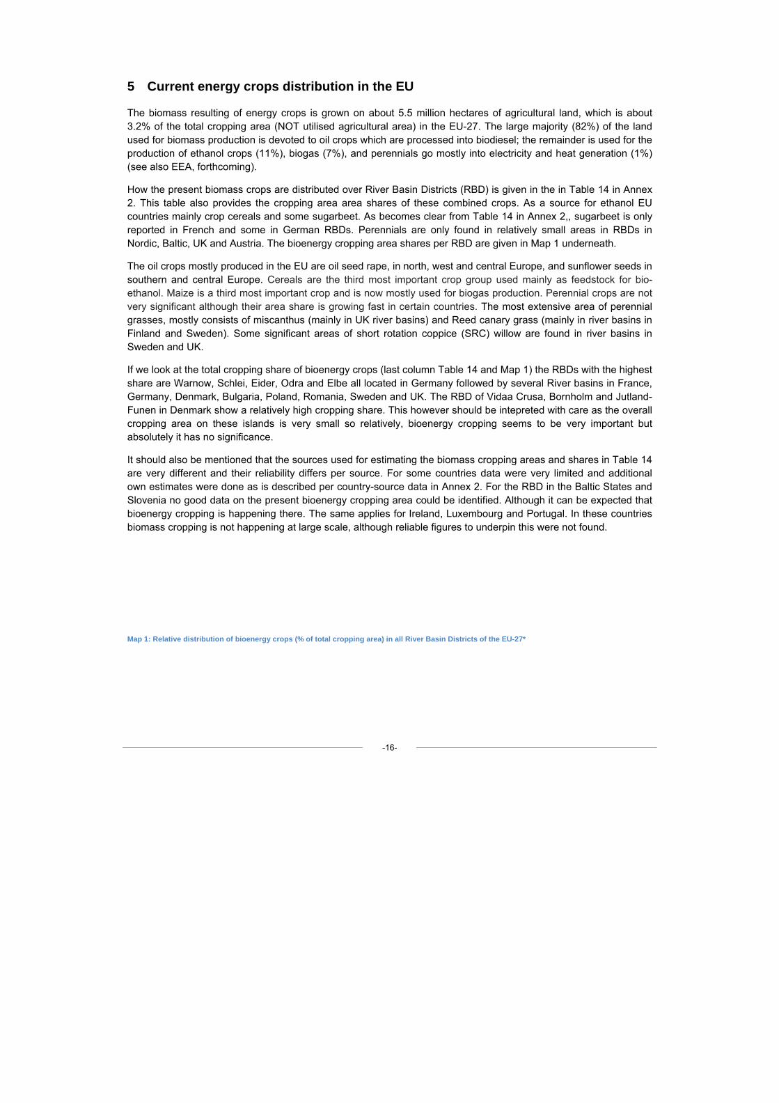
How the present biomass crops are distributed over River Basin Districts (RBD) is given in the in Table 14 in Annex 2. This table also provides the cropping area area shares of these combined crops. As a source for ethanol EU countries mainly crop cereals and some sugarbeet. As becomes clear from Table 14 in Annex 2,, sugarbeet is only reported in French and some in German RBDs. Perennials are only found in relatively small areas in RBDs in Nordic, Baltic, UK and Austria. The bioenergy cropping area shares per RBD are given in Map 1 underneath.

The oil crops mostly produced in the EU are oil seed rape, in north, west and central Europe, and sunflower seeds in southern and central Europe. Cereals are the third most important crop group used mainly as feedstock for bio-ethanol. Maize is a third most important crop and is now mostly used for biogas production. Perennial crops are not very significant although their area share is growing fast in certain countries. The most extensive area of perennial grasses, mostly consists of miscanthus (mainly in UK river basins) and Reed canary grass (mainly in river basins in Finland and Sweden). Some significant areas of short rotation coppice (SRC) willow are found in river basins in Sweden and UK.

If we look at the total cropping share of bioenergy crops (last column Table 14 and Map 1) the RBDs with the highest share are Warnow, Schlei, Eider, Odra and Elbe all located in Germany followed by several River basins in France, Germany, Denmark, Bulgaria, Poland, Romania, Sweden and UK. The RBD of Vidaa Crusa, Bornholm and Jutland-Funen in Denmark show a relatively high cropping share. This however should be intepreted with care as the overall cropping area on these islands is very small so relatively, bioenergy cropping seems to be very important but absolutely it has no significance.

It should also be mentioned that the sources used for estimating the biomass cropping areas and shares in Table 14 are very different and their reliability differs per source. For some countries data were very limited and additional own estimates were done as is described per country-source data in Annex 2. For the RBD in the Baltic States and Slovenia no good data on the present bioenergy cropping area could be identified. Although it can be expected that bioenergy cropping is happening there. The same applies for Ireland, Luxembourg and Portugal. In these countries biomass cropping is not happening at large scale, although reliable figures to underpin this were not found.

Map 1: Relative distribution of bioenergy crops (% of total cropping area) in all River Basin Districts of the EU-27*

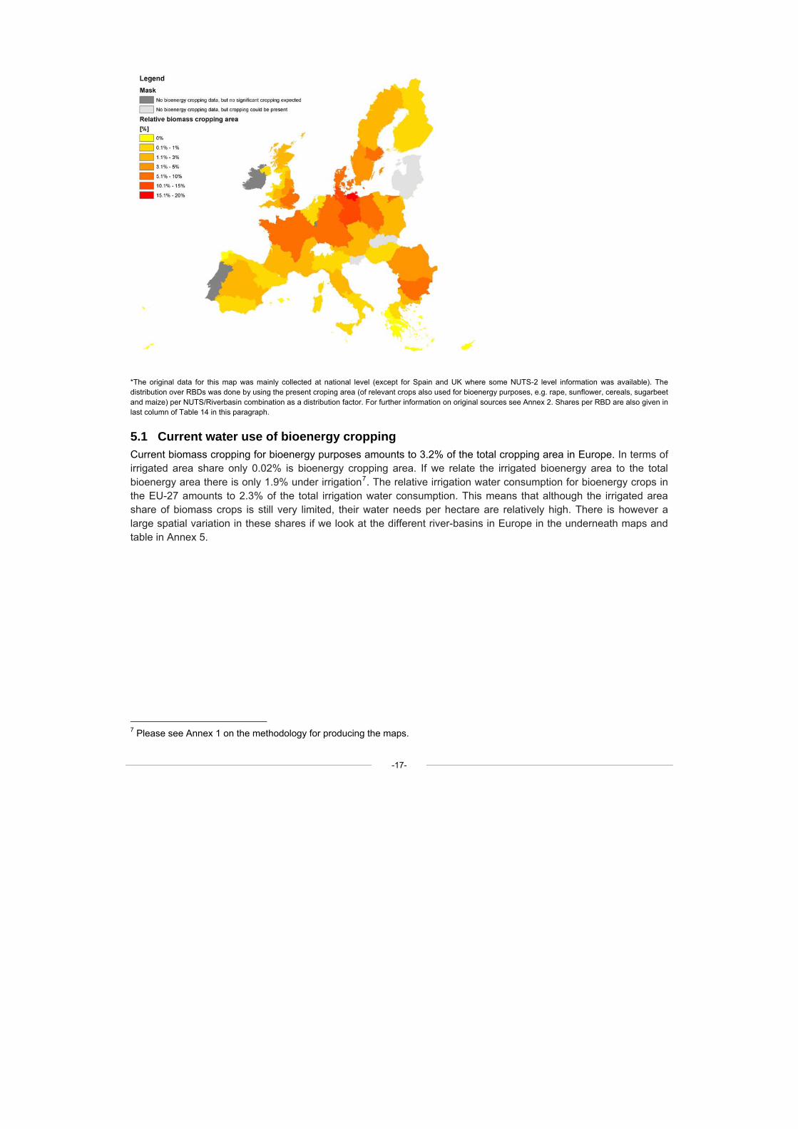
*The original data for this map was mainly collected at national level (except for Spain and UK where some NUTS-2 level information was available). The distribution over RBDs was done by using the present croping area (of relevant crops also used for bioenergy purposes, e.g. rape, sunflower, cereals, sugarbeet and maize) per NUTS/Riverbasin combination as a distribution factor. For further information on original sources see Annex 2. Shares per RBD are also given in last column of Table 14 in this paragraph.

5.1 Current water use of bioenergy cropping Current biomass cropping for bioenergy purposes amounts to 3.2% of the total cropping area in Europe. In terms of irrigated area share only 0.02% is bioenergy cropping area. If we relate the irrigated bioenergy area to the total bioenergy area there is only 1.9% under irrigation7. The relative irrigation water consumption for bioenergy crops in the EU-27 amounts to 2.3% of the total irrigation water consumption. This means that although the irrigated area share of biomass crops is still very limited, their water needs per hectare are relatively high. There is however a large spatial variation in these shares if we look at the different river-basins in Europe in the underneath maps and table in Annex 5.

7 Please see Annex 1 on the methodology for producing the maps.

-17-

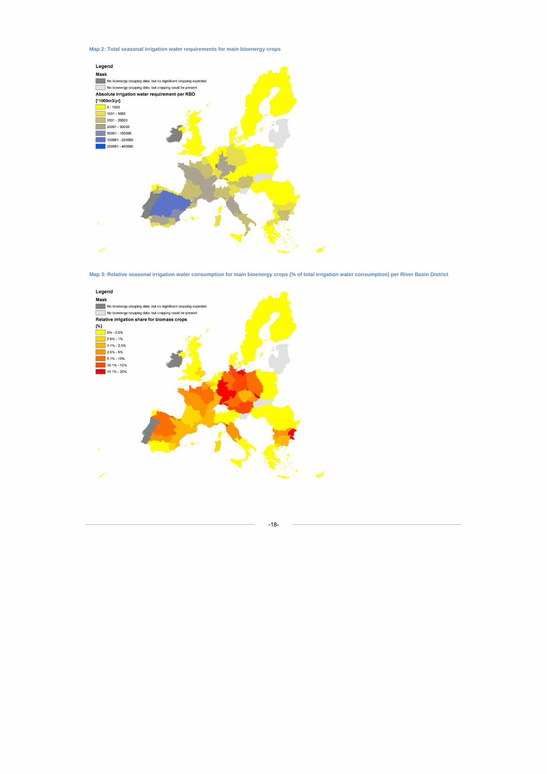
Map 2: Total seasonal irrigation water requirements for main bioenergy crops

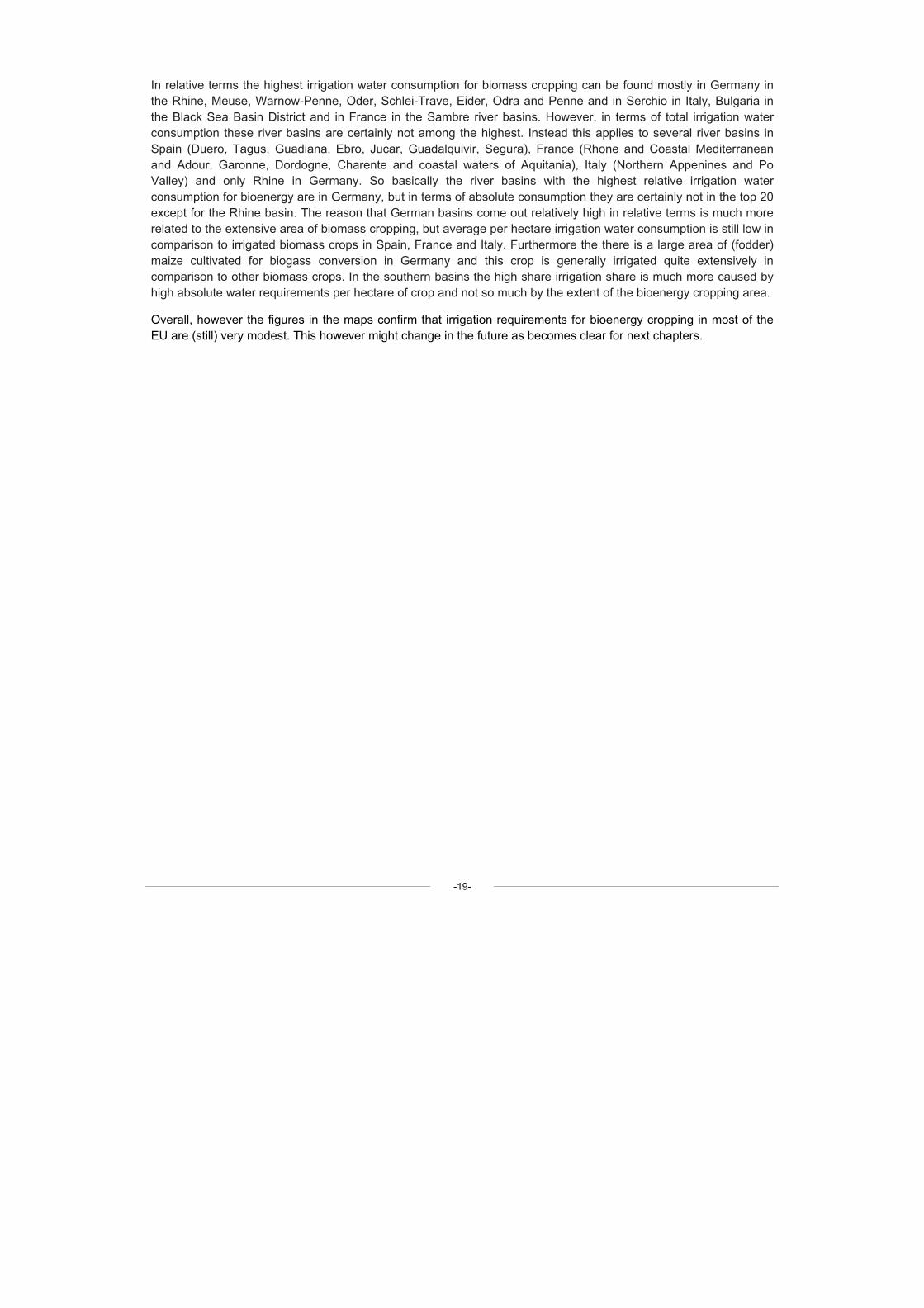
Map 3: Relative seasonal irrigation water consumption for main bioenergy crops (% of total irrigation water consumption) per River Basin District

-18-

-19-

In relative terms the highest irrigation water consumption for biomass cropping can be found mostly in Germany in the Rhine, Meuse, Warnow-Penne, Oder, Schlei-Trave, Eider, Odra and Penne and in Serchio in Italy, Bulgaria in the Black Sea Basin District and in France in the Sambre river basins. However, in terms of total irrigation water consumption these river basins are certainly not among the highest. Instead this applies to several river basins in Spain (Duero, Tagus, Guadiana, Ebro, Jucar, Guadalquivir, Segura), France (Rhone and Coastal Mediterranean and Adour, Garonne, Dordogne, Charente and coastal waters of Aquitania), Italy (Northern Appenines and Po Valley) and only Rhine in Germany. So basically the river basins with the highest relative irrigation water consumption for bioenergy are in Germany, but in terms of absolute consumption they are certainly not in the top 20 except for the Rhine basin. The reason that German basins come out relatively high in relative terms is much more related to the extensive area of biomass cropping, but average per hectare irrigation water consumption is still low in comparison to irrigated biomass crops in Spain, France and Italy. Furthermore the there is a large area of (fodder) maize cultivated for biogass conversion in Germany and this crop is generally irrigated quite extensively in comparison to other biomass crops. In the southern basins the high share irrigation share is much more caused by high absolute water requirements per hectare of crop and not so much by the extent of the bioenergy cropping area.

Overall, however the figures in the maps confirm that irrigation requirements for bioenergy cropping in most of the EU are (still) very modest. This however might change in the future as becomes clear for next chapters.

-20-

6 Impacts of future bioenergy developments on irrigation water demand

Based on the current policy framework, three different storylines have been developed, describing possible future developments of bioenergy cropping and irrigation patterns in Europe. These three storylines are based on several qualitative assumptions mostly based on published (scientific) references. These have been translated further into qualitative assumptions to allow the estimation of future spatial cropping shares and patterns and related irrigation water demand per RBD region. The three scenarios allow a comparison in terms of irrigation water requirements but also in terms of biomass and energy yields.

6.1 The three storylines/scenarios in a nutshell To estimate potential future pressures and impacts on water quantity from increasing cultivation of bioenergy crops at regional level, three different storylines have been developed. These describe alternative evolutions of bioenergy cropping patterns and irrigation policy specifications up to the year 20208. It is important to note that the storylines are based on expert judgments and do not consider economic modelling: The three storylines can be summarised as follows:

• Storyline 1: The overall water consumption for irrigation remains the same as today. While irrigation technologies used become more efficient (less water per ha used), the water saved is used to develop new irrigation areas for food and non food production.

• Storyline 2 is based on the developments set out in the first scenario, but due to an extensive use of Art. 4.7 WFD, new irrigation projects in several Basins and the reestablishment of old irrigation patterns in CEEC is assumed.

• Storyline 3 is also based on the assumptions set out in scenario one, but in those RBD already facing water stress (see Annex 3), a reduction of water abstraction by 40% is required.

As a result of the three storylines, the impact of increasing or limiting the opportunities for irrigated bioenergy cropping on energy potential can be estimated. However, it should be noted that several uncertainties are related to the developed scenarios and their translation into cropping and irrigation shares and irrigation water consumption. The results should therefore be interpreted as possible corridors of development rather then most likely futures. They do however show to what extent policy limitations on irrigation water use may influence the cropped bioenergy potential in the total EU and in different regions.

6.2 Main Drivers influencing the future of bioenergy cropping within the current policy framework

As set out in Section 1.1, the future bioenergy cropping pattern and practice in Europe will strongly depend on how the current policy framework will be further implemented. National renewable action plans are not fully available, making it more difficult to estimate where and how many hectares of targeted biomass crops will be grown in the future. However, this future pattern of bioenergy cropping will clearly depend on:

• Overall development of agricultural and energy markets and related relative prices.

• Local land and water availability,

8 According to the Terms of reference, also development until 2030 should be considered, but after some preliminary investigations it was agreed at the Kick off meeting that such scenarios would not deliver reliable results because of large uncertainties in policy making, technology developments and cropping practices.

-21-

• Technological state of developments,

• Share of available types of biomass converted into the three bioenergy categories (electricity, heating, transport),

• The impacts of climate change in the different regions especially in relation to changes in temperature and precipitation, and

By building on the assessment of previous studies, a further elaboration of the five issues is given underneath. They form the basis for the further specifications of the three storylines elaborated in this study and implemented into real estimates as presented in Section 6.3. More details on how the storyline specifications have been converted into estimates of land and irrigation water requirements and eventual biomass and energy yields are also described in Annex 1 (Sections 3 and 4).

Economic drivers

It is assumed that food and feed production have a higher priority than bioenergy cropping in the future and that this is reflected in market prices. In other words, margins that a farmer can achieve per crop remain higher for food than for bioenergy. Considering this for all scenarios it is assumed that:

• the self-sufficiency rates of Europe for food and feed is fixed for all scenarios and bioenergy crops are only grown on land that is not needed to satisfy this food and feed demand. In this study, the overall land availability for bioenergy cropping is therefore based on the CAPSIM Animlib scenario calculation results, assuming no implementation of bioenergy targets by 2020 but giving indications of the amount and type of land released from agriculture between 2000 and 2020 (see Annex 5);

• the share of costs for labour, water, fuel, feed, fertilizer, seed and other inputs consumed on the farm, and the rental value of farmland and dwellings remains stable; and

• the margins a farmer can achieve on the market remain stable.

• Enough economic incentives are in place to make farmers decide to grow energy crops on released agricultural and set-aside lands.

Land and water availability

Land availability and quality of land will be one important factor influencing the amount and type of cropped biomass feedstock produced in EU regions. Due to the large pressure from the energy sector to achieve the agreed targets and the resulting demand for biomass feedstock, the following assumptions were made with regard to land use changes9:

1) Land released from agricultural food and feed production is used for production of biomass for energy. However, the area that becomes available is first reduced by a share ranging from 0.5–2.0 % for non-agricultural purposes10.

9 As similar approach was used in European Environment Agency (2007). 10 The estimation on future land requirement for non-agricultural uses of released agricultural lands was made as follows; 0.5% Estonia, Latvia, Lithuania, Bulgaria, Turkey, Romania; 1.0% Hungary, Slovakia, Poland, Spain, Greece, Cyprus, Slovenia, Portugal, Czech Republic, Finland, Sweden, Ireland, Austria; 1.5% France, Denmark, Luxembourg, Italy, Malta; 2.0% Germany, United Kingdom, Belgium, Netherlands.

-22-

2) In addition it is also assumed that in countries for which statistical or published evidence is given of high (historical) land abandonment figures (based Pointereau et al., 2008) some more land is added to the released land pool (according to CAPSIM Animlib scenario calculations) that is expected to become available for biomass cropping. This additional abandoned land will be a maximum of 20% of the CAPSIM released land resource. This will only be the case for most CEEC countries and some Mediterranean countries. This land resource is added to the set-aside/fallow land pool.

3) Former set aside land is used for production of bioenergy. Part of the set aside land has already been used by farmers to grow bioenergy crops on in the last couple of years. It is assumed that this practice will continue even under the new conditions set out under the CAP Health Check.

4) Land that is already in use for biomass crop production in 2000 will remain in the future and will therefore be part of the future potential land.

5) It is assumed that land released in the arable category has a higher chance to be converted to biomass cropping, than released set-aside/fallow land. To implement this 100% of the released arable land (after correction for non-agricultural uses) is expected to be converted and only 50% of the released set-aside/fallow land pool.

In Annex 1, Table 13 the estimate of additional land for biomass cropping is presented by RBD in 2020 (derived from CAPSIM model runs and additional assumptions specific to this study, see Annex 1, Section 4). As becomes clear the RBD with the largest land potential are the Romanian and Bulgarian part of the Danube, the Vistula and Odra in Poland, the Nemunas in Latvia and the Elbe in Germany. In the south this applies to the North and South Apennines and the Po basin in Italy and the Duero, Ebro and Guadiana in Spain.

It is assumed that only the released arable and set-aside land are really available for biomass cropping. The released grassland cannot be used directly as ploughing-up grassland would lead to an unacceptable large release of carbon (Johnson and Roman, 2008) which can never be recovered by bioenergy cropping.

Furthermore, a maximum is set on the amount of land per region that can be used for biomass cropping by 2020. This maximum is set on 20% of the total 2020 cropping area as it cannot be expected that within 13 years time enough economic and technical means are available to convert a higher share of land.

This means that in 2020 almost 18 million hectares of agricultural land are expected to be potentially available for non-agricultural purposes. About one third consists of land that was already in use for biomass cropping in 2007/2008 (see Chapter 5) and the other 66% will be additionally available. The scenario specifications will determine how much of this potential land will also be converted to bioenergy cropping land (see Section 6.3 and 6.4).

Water availability

Water availability for irrigation can be a major constraint in many areas. The available irrigation water is influenced by the total water availability of a region, the abstraction needs of other sectors and losses in the supply system. In the WATER GAP project (Flörke and Alcamo, 2004) for Europe, water availability was estimated for the year 2020 as well as potential consumption rates. The WATER GAP assumptions on total water availability, sectoral water use for industry, domestic use form also the baseline for this study. The water abstraction for irrigation varies in each scenario (see Section 6.3). In all cases it is assumed that irrigation patterns develop firstly on current rain fed agricultural land and secondly on abandoned land and thirdly on set aside land.

Per scenario different amounts of (additional) irrigation water volumes per region will be available for biomass cropping. It is assumed however, that if irrigation water volumes remain stable for a RBD the irrigation share of the biomass cropping areas that continue to exist between 2007 and 2020 remain stable. If additional irrigation water is

-23-

available in a RBD (according to the scenario specification (see Section 6.3) this will allow some additional irrigation in biomass crops. However most of the water (at least 2/3) that becomes available for irrigation will be used for feed and food crops and the rest maybe used for biomass crops.

Furthermore, biomass crops will only be irrigated if this leads to a significantly higher yield in that typical location and/or if this crop can only deliver an economic yield in that location with irrigation (e.g. certain perennials in Mediterranean regions).

To estimate the water availability in 2020 and to put the bioenergy irrigation water needs in a relative position the Wriedt et al. (2008) figures are used as the basis (in 2003) from which extrapolations on irrigation water availability in 2020 are made. Wriedt et al. (2008) uses data of 2003 to estimate the present regional distribution of irrigation patterns and water consumption. It was also considered to use the future predictions on water consumption from the „WATERGAP“ model (Flörke and Alcamo, 2004) but there are several reason why it was preferred to use the Wriedt et al. (2008) database above the „WATERGAP“ model outcomes:

1) Wriedt et al. (2008) data are more spatially detailed (10*10 km grid) then the „WATERGAP“ base data and scenario results. „WATERGAP“ uses 0.5° by 0.5° minutes grid cells (250 km*250 km grids in EU).

2) Wriedt et al. (2008) uses more recent and spatially detailed base data from Eurostat and national sources (2003-2005) to map the baseline and fit it to the present cropping pattern while Flörke and Alcamo (2004) build most of their database from 2000 sources.

3) Irrigation water use predictions in the scenario need to be compared to the present situation. For comparison Wriedt et al. (2008) is used as a starting point for both situations. If „WATERGAP“ would have been used no good comparison was possible.

4) „WATERGAP“ predicted extend of irrigated area up-to 2030 and our study only looks at 2020 situation.

5) Driving forces for change in irrigation are part of our own storyline assumptions and they do not match with the ones taken in the „WATERGAP“ assessment.

6) However, assumptions provided by „WATERGAP“ study on water use efficiency improvements for the future were also used in our study. They were however applied to our Wriedt et al. (2008) baseline situation.

In spite of all these differences it is interesting to place the main outcomes of our study in the context of the „WATERGAP“ model predictions. This will be done in Section 6.5 of this study.

Technological developments (2nd generation of biofuels)

The development of second generation biofuels is dependent on technological development, and technologies influences the type of feedstock needed by processors. 1st generation biofuels production is already in place, the technology is mature and less expensive than the conversion of lignocellulosic compounds for the production of ethanol (Gray et al., 2006).

The processes for developing second-generation biofuels are much more complex than those used for first-generation fuels and both the technologies and the logistics are still at a very early stage. While natural oils are extracted from the plants to produce first-generation biofuels, second-generation processes, which work with waste and ‘woody’ materials, require complex catalysis and chemical alteration procedures to create the oils in the first place. So far, only certain small experimental or demonstration plants exist and production is nowhere near to being started on a commercial level.

According to a study on behalf of the JRC, it is unlikely that 2nd generation biofuels will be competitive with 1st generation by 2020 (Edwards et al., 2007). The techno-economic analysis indicates that 2nd generation biofuels will

-24-

be much more expensive than first generation biofuels. Costs are dominated by investment costs of the plant. In order to arrive at overall production costs competitive with first generation biofuels, one would have to assume very significant “learning” to reduce the capital cost by 2020.

This slow technological change is also influenced by the fact that the integration of new crops into traditional farming practices by farmers is low. This is why farmers first opt to go for food and feed production, and bioenergy crops are more likely to appear in places where land is released. Furthermore, the readiness to change traditional farming practices is low, which makes it more likely for farmers to take up rotational arable biomass crops than perennials, unless land that is available has a lower quality and is less suited for rotational arable cropping. Perennials, which require farmers to take land out of their rotation for 15 to 20 years, are not expected and that is why perennial are more likely to be placed on the lower quality lands which are expected to become available through the taking into use of set-aside and abandoned land categories by 2020. Perennials produced by 2020 are not so much seen as feedstock for the 2nd generation biofuels, but much more for production of bio-electricity and heat.

Share of available types of biomass converted into the three bioenergy categories

As stated in Chapter 2, biomass feedstock can be converted into transport fuels, heat and electricity. The share of these three energy types produced from bioenergy crops in the overall energy system has a direct influence on cropping patterns (e.g. the conversion of (woody) biomass to electricity and heat is more energy and GHG efficient than the conversion to biofuels). Considering the requirements set out under the Renewable Energy Directive, it is expected that biomass based heat and electricity applications will become considerably more important. However, as the Directive also calls for a binding share of renewable energy in the transport sector of 10% by 2020, it is assumed that this will require strong involvement of agriculture feedstocks produced on irrigated and non irrigated land. For each scenario a specific development of the irrigated area share and water consumption is assumed.

Climate change

According to a recent report for the European Commission (Iglesias et al., 2007), the climatic impacts presented in Map 4 are forecasted for the four agri-climatic zones in EU-27. In order to adapt to these new challenges, agricultural water use has to be optimised, especially in central and southern European water-scarce regions. Northern regions will face an increase in nutrient losses and erosion due to increased precipitation, with negative impacts such as eutrophication of aquatic ecosystems. Regional planning, landscape design and farming techniques are important tools in such an adaptation process.

However it should be noted that the long term changes (e.g. increase in temperature) due to climate change until 2020 are expected to be moderate. The main medium term impact will come from a higher frequency of extreme weather events such as very hot summers with risks of water shortages, heavy rainfalls with subsequent flooding, heavy storms with damages and risks for floods and coastal erosion (European Commission, 2009).

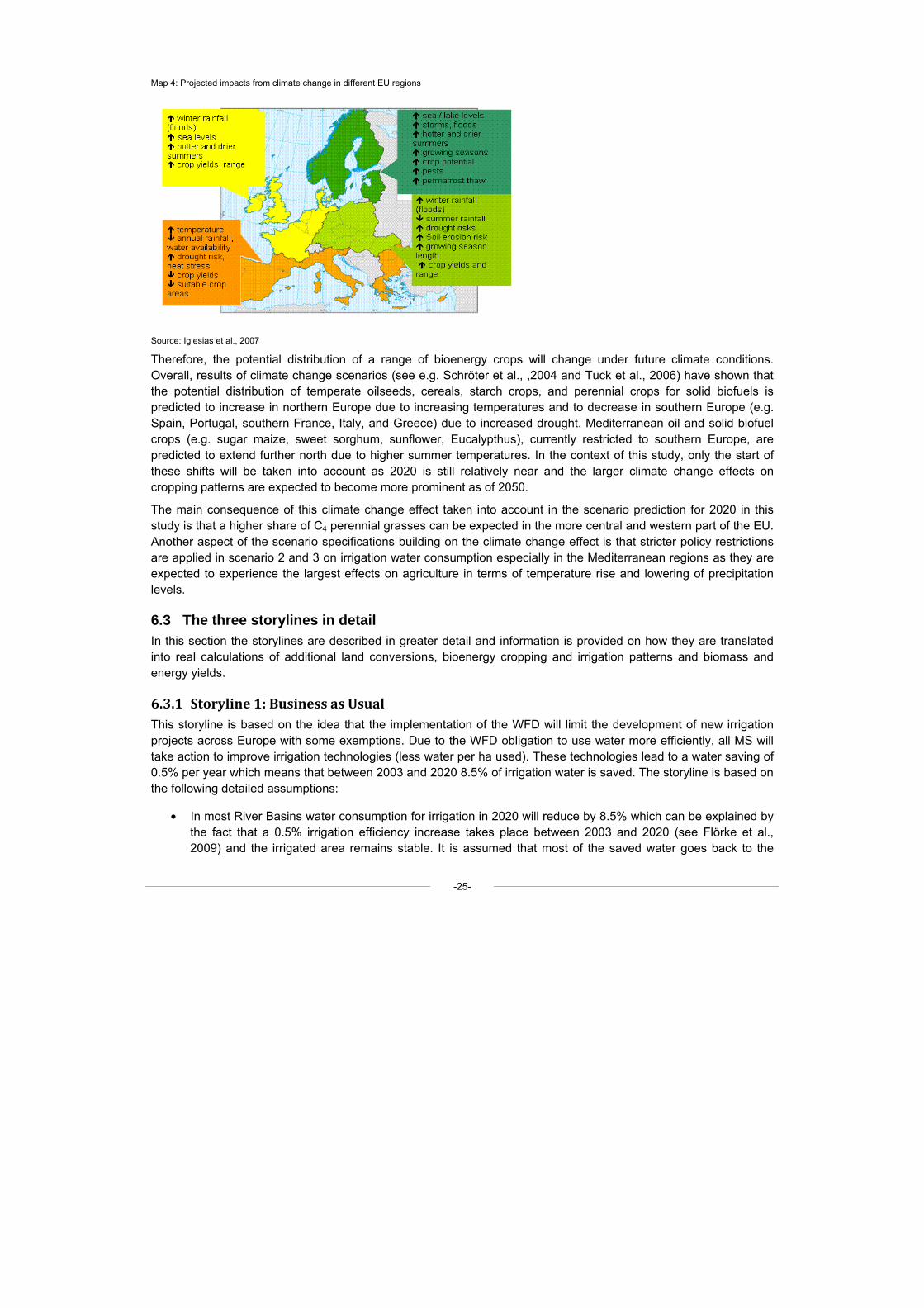
Map 4: Projected impacts from climate change in different EU regions

Source: Iglesias et al., 2007

Therefore, the potential distribution of a range of bioenergy crops will change under future climate conditions. Overall, results of climate change scenarios (see e.g. Schröter et al., ,2004 and Tuck et al., 2006) have shown that the potential distribution of temperate oilseeds, cereals, starch crops, and perennial crops for solid biofuels is predicted to increase in northern Europe due to increasing temperatures and to decrease in southern Europe (e.g. Spain, Portugal, southern France, Italy, and Greece) due to increased drought. Mediterranean oil and solid biofuel crops (e.g. sugar maize, sweet sorghum, sunflower, Eucalypthus), currently restricted to southern Europe, are predicted to extend further north due to higher summer temperatures. In the context of this study, only the start of these shifts will be taken into account as 2020 is still relatively near and the larger climate change effects on cropping patterns are expected to become more prominent as of 2050.

The main consequence of this climate change effect taken into account in the scenario prediction for 2020 in this study is that a higher share of C4 perennial grasses can be expected in the more central and western part of the EU. Another aspect of the scenario specifications building on the climate change effect is that stricter policy restrictions are applied in scenario 2 and 3 on irrigation water consumption especially in the Mediterranean regions as they are expected to experience the largest effects on agriculture in terms of temperature rise and lowering of precipitation levels.

6.3 The three storylines in detail In this section the storylines are described in greater detail and information is provided on how they are translated into real calculations of additional land conversions, bioenergy cropping and irrigation patterns and biomass and energy yields.

6.3.1 Storyline 1: Business as Usual This storyline is based on the idea that the implementation of the WFD will limit the development of new irrigation projects across Europe with some exemptions. Due to the WFD obligation to use water more efficiently, all MS will take action to improve irrigation technologies (less water per ha used). These technologies lead to a water saving of 0.5% per year which means that between 2003 and 2020 8.5% of irrigation water is saved. The storyline is based on the following detailed assumptions:

• In most River Basins water consumption for irrigation in 2020 will reduce by 8.5% which can be explained by the fact that a 0.5% irrigation efficiency increase takes place between 2003 and 2020 (see Flörke et al., 2009) and the irrigated area remains stable. It is assumed that most of the saved water goes back to the

-25-

-26-

environment. Only for the River Basins in Portugal, Spain, Italy, south UK, Bulgaria and Romania11. the irrigation water savings are used to develop new or re-activate former irrigation areas (no decrease or increase in water consumption is expected in these basins) for additional food, feed and biomass crops. It is assumed that more water will be used for food crops for two reasons: a) Food production remains more important than bioenergy crops and b) the water will be mainly used to irrigate “high value crops” such as e.g. fruits, vegetables or cotton. The share is assumed to be 1/3 of additional water for bioenergy crops and 2/3 to food crops. The additional water for bioenergy goes for 50% to rotational arables and 50% to perennials.

• For the bioenergy crop mix it is assumed that the type of released land dictates the mix of rotational arable and perennial crops per region. All rotational crops are placed on the released arable land which is the ‘best’ soil, an can only be placed on a maximum of 20% of the land in the set-aside-abandonment land category assumed to be taken into production. The rest of the land in this last category will go to perennials which is certainly realistic in countries like Sweden, Finland, UK and the Baltic states where national documents on the future developments of bioenergy cropping show that strong incentives to grow perennials will be set.

6.3.2 Storyline 2: Increased irrigation water demand. Storyline 2 assumes that the demand for bioenergy will push new irrigation projects in several European regions. The following developments are assumed:

• In Italy, Malta, Greece, Portugal, RB in Spain which are not facing water stress at the moment12 south UK and four of the CEEC (Hungary, Romania, Bulgaria, Poland), the irrigation area and the irrigation water demand is predicted to grow. Due to the political and economic transformations in the 1980s in most of the CEEC countries, the irrigated areas have diminished drastically but there are several plans to reactivate and/or extend these areas again in order to improve market competition (Dirksen, Huppert, 2006). It is assumed that the increase in irrigated water abstraction will be as specified in the table below. Also irrigation efficiency increases 0.5% per year (based on Flörke et al., 2009). The saved water will be used to develop new irrigation areas in order to supply the food (2/3 of saved water) and bioenergy demand (1/3 of saved water).

11 According to the Portuguese Rural development program a new irrigated area is planned. In the case of Romania and Bulgaria old existing infrastructure is envisaged to be reactivated. In the case of Sweden, UK and Finland it is expected that due to more favorable climatic conditions the agricultural sector will boost and new irrigation systems will be established. 12 As the Spanish law gives the highest priority to water supply to public it is assumed that in RB which are already facing water stress, no new irrigation projects will be allowed.

-27-

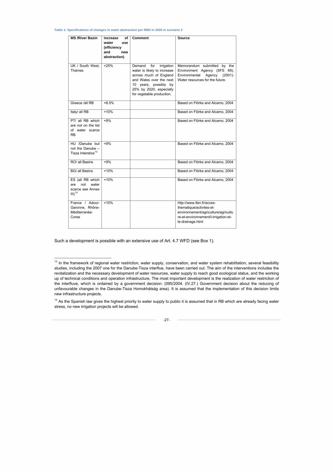
Table 1: Specifications of changes in water abstraction per RBD in 2020 in scenario 2

MS /River Basin increase of water use (efficiency and new abstraction)

Comment Source

UK / South West, Thames

+25% Demand for irrigation water is likely to increase across much of England and Wales over the next 10 years, possibly by 25% by 2020, especially for vegetable production.

Memorandum submitted by the Environment Agency (SFS 69), Environmental Agency (2001): Water resources for the future.

Greece /all RB +8.5% Based on Flörke and Alcamo, 2004

Italy/ all RB +10% Based on Flörke and Alcamo, 2004

PT/ all RB which are not on the list of water scarce RB

+9% Based on Flörke and Alcamo, 2004

HU /Danube but not the Danube –Tisza Interstice13


RO/ all Basins +9% Based on Flörke and Alcamo, 2004

BG/ all Basins +10% Based on Flörke and Alcamo, 2004

ES (all RB which are not water scarce see Annex III)14


France / Adour-Garonne, Rhône-Méditerranée-Corse

+10% http://www.ifen.fr/acces-thematique/activites-et-environnement/agriculture/agriculture-et-environnement/l-irrigation-et-le-drainage.html

Such a development is possible with an extensive use of Art. 4.7 WFD (see Box 1).

13 In the framework of regional water restriction, water supply, conservation, and water system rehabilitation, several feasibility studies, including the 2007 one for the Danube-Tisza interflue, have been carried out. The aim of the interventions includes the revitalization and the necessary development of water resources, water supply to reach good ecological status, and the working up of technical conditions and operation infrastructure. The most important development is the realization of water restriction of the interfluve, which is ordained by a government decision: (095/2004. (IV.27.) Government decision about the reducing of unfavourable changes in the Danube-Tisza Homokhátság area). It is assumed that the implementation of this decision limits new infrastructure projects. 14 As the Spanish law gives the highest priority to water supply to public it is assumed that in RB which are already facing water stress, no new irrigation projects will be allowed.

-28-

• For River Basins in Finland, Sweden, Denmark, Ireland, Belgium, Austria, Germany, the Netherlands, Czech Republic, Slovakia, Slovenia, remaining France and Spain, Cyprus, in the Baltic States water abstraction for irrigation is expected to reduce by 8.5% (2003-2020) due to efficiency increase (0.5% per annum as set out by Flörke and Alcamo, 2004). Further, as climate change effects are not predicted to take extreme changes by 2020 (See e.g. Tuck et al., 2006 and Flörke, et al., 2009). No additional irrigation is needed to keep agricultural production and yields at stable levels. Furthermore, in several of these River Basins the irrigable areas has already been fully explored

• For the bioenergy crop mix it is assumed that the type of released land dictates the mix of rotational arable and perennial crops per region. All rotational crops are placed on the released arable land which is the ‘best’ soil, an can only be placed on a maximum of 20% of the land in the set-aside-abandonment land category assumed to be taken into production. The rest of the land in this last category will go to perennials. Additional irrigation water, if available in 2020 can go for 1/3 to bioenergy cropping which will be distributed for 50% to rotational arables and 50% to perennials.

6.3.3 Storyline 3: Water saving scenario – implications for the bioenergy targets Storyline 3 assumes that the EU is taking action in the area of water saving. The storyline is based on the following detailed assumptions:

• All River Basins currently facing water stress (see Annex 3) have to reduce water abstraction for irrigation by 40%15. As high value crops will be irrigated first bioenergy crops will be irrigated to a minimal. This applies also to the bioenergy areas that were irrigated in 2007 and that have continued to remain in production. In river basins of Bulgaria, Romania, Hungary, which are not expected to be water-stressed an increase in irrigation area and water abstraction (+5% in 2020) is expected in order to ensure competitive agriculture. For the remaining MS/River Basins the irrigation water abstraction will also reduce as efficiency is improving (0.5% a year (2003-2020)) and the irrigated area is assumed to remain stable. The savings of 8.5% for this period will mostly go back to the environment and a small share to serve additional domestic needs.

• The crop mix is estimated to be the same as in storyline 1 and 2, but in the Mediterranean zone less perennials will be grown given the fact that these crops are expected to only delivering economic yields if irrigated under strong arid circumstances (Christou et al., 2004). As the overall water abstraction for irrigation has to be reduced, the focus of irrigation in these regions cannot be expected to be towards perennials as “high value crops” will be prioritised first (Dworak et al., unpublished). This means that perennials are not expected to be grown so wide spread as in the other 2 storylines in the Mediterranean under this storyline. This also means that under this storyline in some regions, where the amount of released land is strongly concentrated in the low quality category, e.g. the set-aside-abandoned land category, not all additional land can be used for biomass cropping. The total additional biomass cropping area share may therefore turn out to be relatively lower.

In the remaining countries perennials are not considered to be irrigated to a large extend as the total irrigated area remains stable (no large climate change effect expected for these regions by 2020) and all water saved due to more efficient irrigation systems will be returned to the environment.

6.3.4 Implementation of the storyline specifications into calculation of irrigation requirements and biomass and energy yields

Implementation of storylines is done in the first instance at the level of NUTS-2 areas, since this is the level at which most of the input information is readily available or to which it can easily be allocated (if only national data available).

15 This value was provided by Commission services based on the 2007 Communication on water scarcity and droughts.

-29-

The CAPSIM data on land availability are for example provided at National level and redistributed to regions according to crop weighting factors obtained from Wriedt et al. (2008) per NUTS-2 area. The same applies to most information on present and future biomass cropping mix derived from reports and policy documents.

The implementation of the storyline into quantitative results involves the following steps, which are described in greater detail in Annex 1.

Step 1: Estimation of land availability according to CAPSIM and desaggregation of land availability from national to regional (NUTS-2) level. CAPSIM predicts the land need in 2020 for arable, set-aside-fallow, grasslands and permanent crops. By comparing the land use of these crop categories between 2000 and 2020 an estimate can be made of types of land released in these categories. This then results into a potential land availability which needs to be translated further to an estimate of land that is likely to be converted to biomass cropping.

Step 2: Estimation of 2020 bioenergy crop mix (see Annex 7). This mix is selected according to a combination of information on:

• Present biomass cropping mix (see Chapter 5)

• Future biomass crop mix as specified in national Rural Development Plans or other national documents.

• The environmentally compatible crop mix as specified in the EEA (2008) study on the environmentally compatible biomass potential.

• The irrigation water availability. Certain crops, such as perennials in the Southern Mediterranean will only deliver economic yields if irrigation is applied and certainly in scenario 3 this will lead to a more limited distribution of this cropping type.

• Type of land availability. Rotational arable crops have higher requirements for soil quality and can only be grown on land that was released in the arable category. Perennials are more likely to be grown on lower quality of land, e.g. land formally identified as set-aside or abandoned. So if a large proportion of the released land consists of these last 2 categories the perennial area share will be higher.

Step 3: Distribution of the total biomass crop mix (identified in step 2) over the total land area released per region (as predicted in step 1). This distribution will determine the eventual total cropping area used for biomass crop per scenario and per region. In this step the final crop mix is determined per region, while in step 2 the average crop mix is still determined at the national level. In this step the overall crop mix is fitted to the production circumstances in a region and land quality. Crops that do not fit with the regional bio-climatic circumstances are not allocated to that region, even if they are part of the national bioenergy crop mix (determined in step 2).

Step 4: Identification of the regions that are water scarce and the ones where additional irrigation water will be available for biomass cropping. Calculate per region (NUTS-2) the total amount of additional water availability, given scenario specifications, to be used for food and feed and for biomass cropping. And in the water scarce regions in the case of scenario 3, the amount of water that is no longer available for irrigation because of water saving measures.

Step 5: (only applicable to storyline 1 and 2) Identify per region whether there is room for irrigation of biomass crops and what amount of water can be used for these crops. It is assumed that in the RB where irrigation area can increase (specified per scenario) 1/3 of the water that becomes available can be used for biomass cropping. The distribution of irrigation water available for biomass cropping should be distributed over crops but only if this leads to a significantly higher yield in that typical location. For rotational arable crops, which in principle get 50% of the available addition water for bioenergy, irrigation is only possible if irrigation practice is already common for this crop in that region and it is among the most water efficient irrigated bioenergy crops. For perennials, who also get 50% of

-30-

irrigation water available, a prioritization is to the most water efficient type which can be a C3 or a C4 perennial grass, depending on the location in the EU. So high yielding (Tons DM/ha) and very water efficient crops (Liters/ton DM) get higher priority in irrigation.

Step 6: Disaggregation of all calculated information from the region levels (NUTS-2) to the grid levels in order to aggregate the grid level information to the total RBD region levels and make total calculations.

Step 7: Mapping of information derived from Step 6 and calculate results at RBD level. This results in the information presented in the next section.

6.4 Uncertainties in the storyline development The development of scenarios or storylines is always depending in assumptions and predictions of future developments. It is important to note that the future development of bioenergy is currently highly uncertainty. Even if political targets are agreed the ways of achieving these targets are currently not fully known. MS are in the process of drawing their action plans indicating how to achieve the renewable and biofuel targets. These plans may differ widely from the assumptions made in this study in particular on land availability and crop mixes. More environmental friendly approaches (e.g. limiting the use of grassland) might be considered.

Land can be available in many places, but it will be determined by market forces, stimulation measures and willingness of the farmers whether this will really lead to a conversion into biomass production. Furthermore, how much of the biomass will eventually be cropped within the EU is an even bigger unknown. Integrated modelling efforts have only recently started to get realistic predictions on this matter.

Further the current CAP regime will end in 2013. The future regime can not predict at this stage. This is related to several uncertainties such as budgets for bioenegy cropping or importance of environmental concerns.

A further uncertainty is the impact of climate change on the regional level. Several uncertainties limit the accuracy of current projections. One relates to the degree of temperature increase and its geographic distribution. Another pertains to the concomitant changes likely to occur in the precipitation patterns that determine the water supply to crops, and to the evaporative demand imposed on crops by the warmer climate. There is a further uncertainty regarding the physiological response of crops to enriched carbon dioxide in the atmosphere.

Another very uncertain factor is whether and to which part of the biomass cropping will be done under rain-fed and irrigated management in every region. This again is a matter of access to water, presence of irrigation infrastructure and economics. In many places in Europe additional irrigation will not lead to a very large increase in yields, but in the South irrigation can make a large difference. Whether irrigation will be practiced and whether it will be of significant influence on the decision to start cropping biomass or not in every region still requires much social-economic research. Agricultural micro-economics have shown in the past that only small differences in gross margins, caused e.g. by use of irrigation, could make farmers decide to apply a certain crop under a certain management practice. In this study this issue has not been taken into account at all. The only aspect which was involved was access to irrigation water and infrastructure.

Finally the development of EU and world market for agricultural products and energy might develop different than assumed in the storyline. Prices might change, imports might differ.

6.5 Scenario results Given the assumption that the 2007/2008 cropping area share remains stable until 2020 and that bioenergy cropping is stimulated sufficiently to make the conversion of released agricultural land attractive enough, it was estimated that the overall bioenergy cropping area will become 4.5 times larger between now and 2020 (see Table 2). The relative bioenergy cropping area share will only show a modest increase from 3% to almost 6%, depending on the scenario (Table 2). This is of course a relative increase as it will also go together with an additional overall increase in the

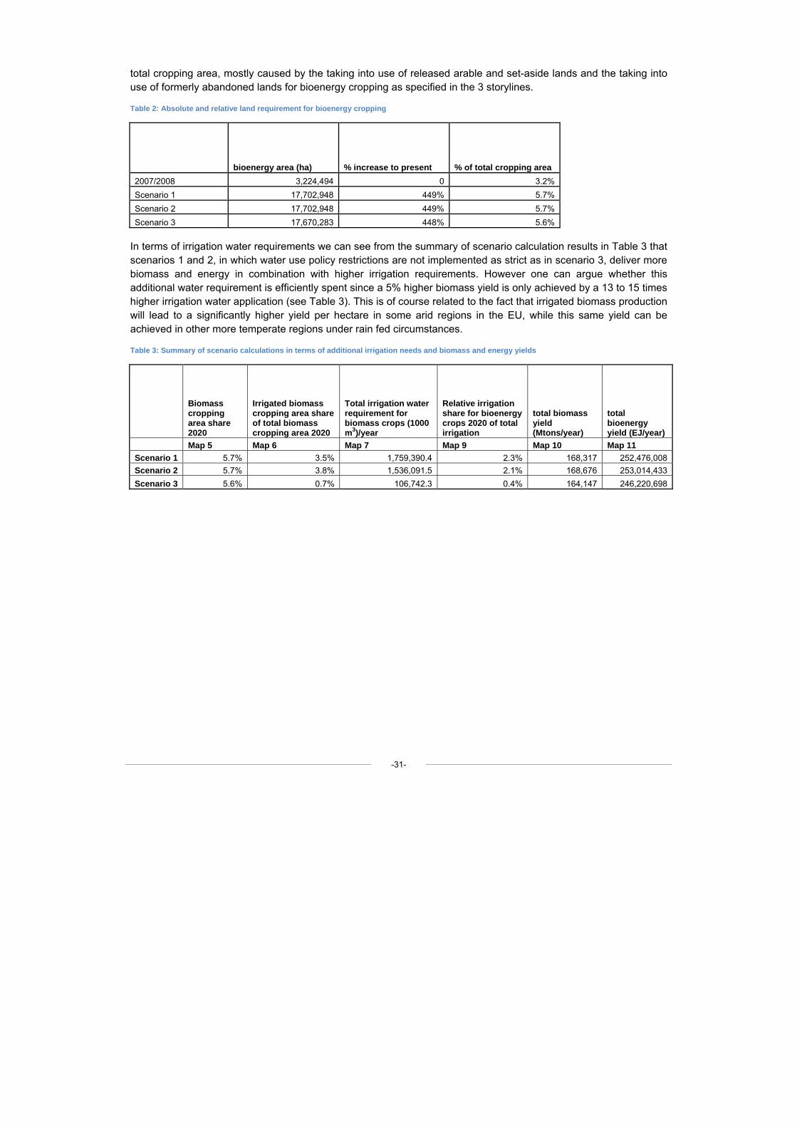
-31-

total cropping area, mostly caused by the taking into use of released arable and set-aside lands and the taking into use of formerly abandoned lands for bioenergy cropping as specified in the 3 storylines.

Table 2: Absolute and relative land requirement for bioenergy cropping

bioenergy area (ha) % increase to present % of total cropping area 2007/2008 3,224,494 0 3.2%Scenario 1 17,702,948 449% 5.7%Scenario 2 17,702,948 449% 5.7%Scenario 3 17,670,283 448% 5.6%

In terms of irrigation water requirements we can see from the summary of scenario calculation results in Table 3 that scenarios 1 and 2, in which water use policy restrictions are not implemented as strict as in scenario 3, deliver more biomass and energy in combination with higher irrigation requirements. However one can argue whether this additional water requirement is efficiently spent since a 5% higher biomass yield is only achieved by a 13 to 15 times higher irrigation water application (see Table 3). This is of course related to the fact that irrigated biomass production will lead to a significantly higher yield per hectare in some arid regions in the EU, while this same yield can be achieved in other more temperate regions under rain fed circumstances.

Table 3: Summary of scenario calculations in terms of additional irrigation needs and biomass and energy yields

Biomass cropping area share 2020

Irrigated biomass cropping area share of total biomass cropping area 2020

Total irrigation water requirement for biomass crops (1000 m3)/year

Relative irrigation share for bioenergy crops 2020 of total irrigation

total biomass yield (Mtons/year)

total bioenergy yield (EJ/year)

Map 5 Map 6 Map 7 Map 9 Map 10 Map 11 Scenario 1 5.7% 3.5% 1,759,390.4 2.3% 168,317 252,476,008Scenario 2 5.7% 3.8% 1,536,091.5 2.1% 168,676 253,014,433Scenario 3 5.6% 0.7% 106,742.3 0.4% 164,147 246,220,698

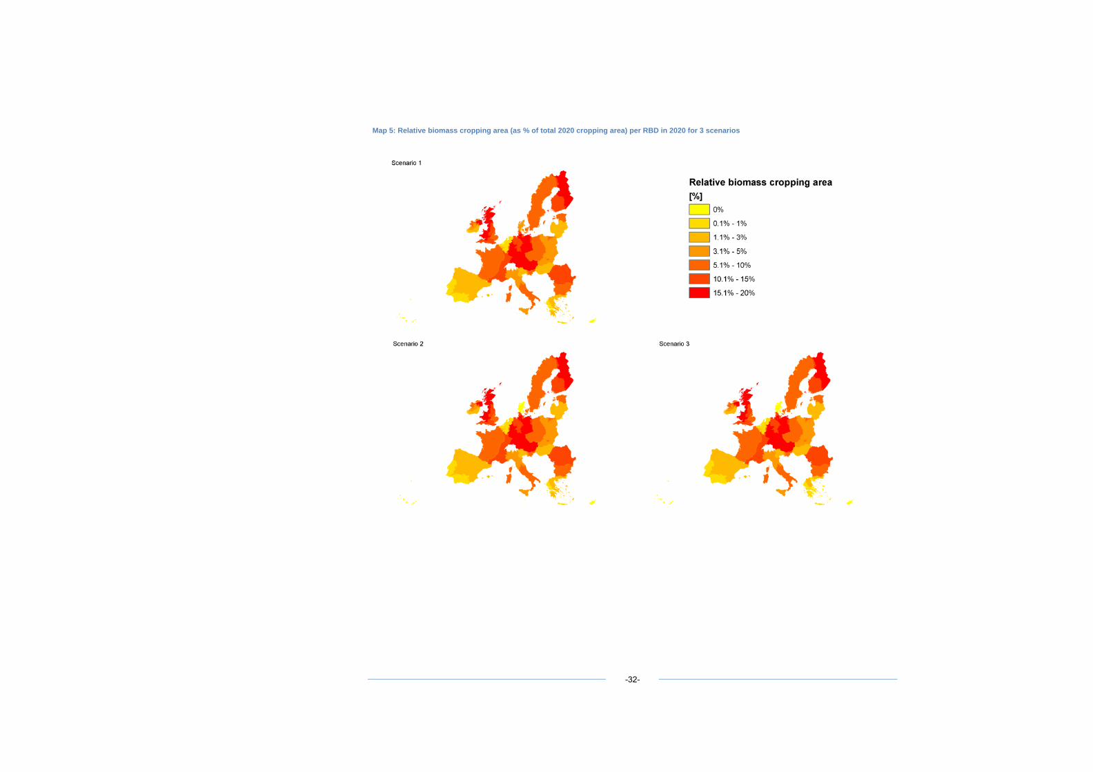
Map 5: Relative biomass cropping area (as % of total 2020 cropping area) per RBD in 2020 for 3 scenarios

-32-

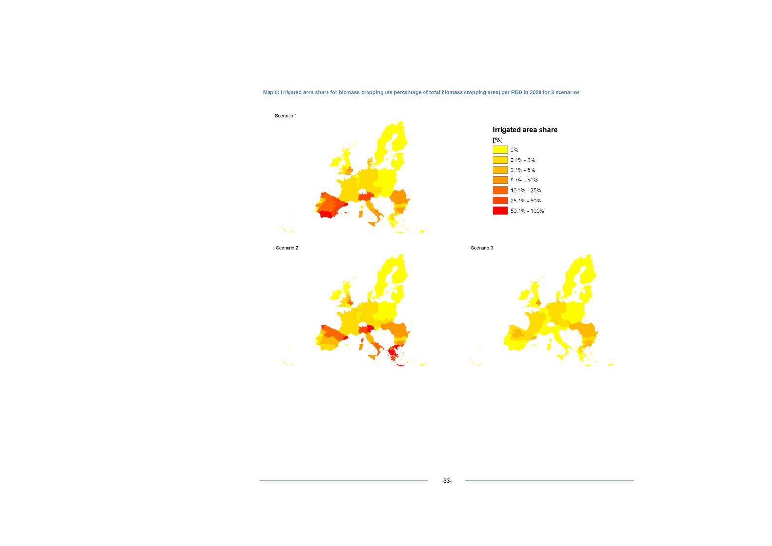
Map 6: Irrigated area share for biomass cropping (as percentage of total biomass cropping area) per RBD in 2020 for 3 scenarios

-33-

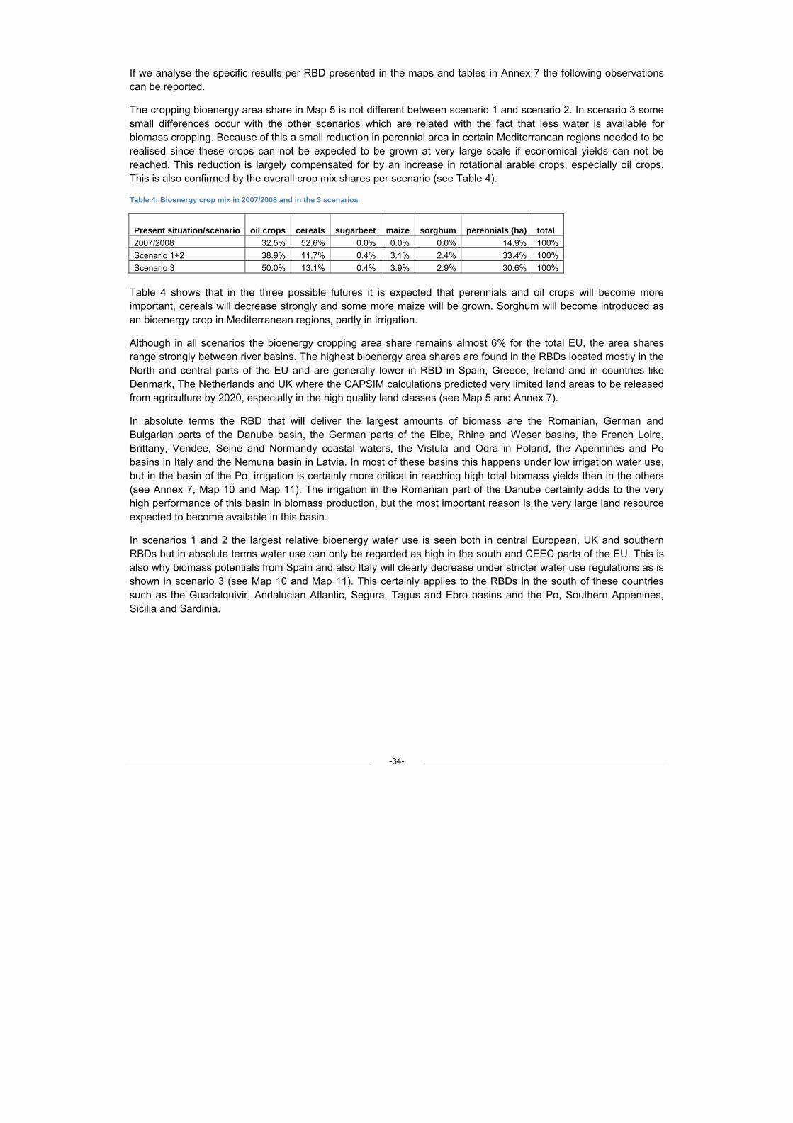
-34-

If we analyse the specific results per RBD presented in the maps and tables in Annex 7 the following observations can be reported.

The cropping bioenergy area share in Map 5 is not different between scenario 1 and scenario 2. In scenario 3 some small differences occur with the other scenarios which are related with the fact that less water is available for biomass cropping. Because of this a small reduction in perennial area in certain Mediterranean regions needed to be realised since these crops can not be expected to be grown at very large scale if economical yields can not be reached. This reduction is largely compensated for by an increase in rotational arable crops, especially oil crops. This is also confirmed by the overall crop mix shares per scenario (see Table 4).

Table 4: Bioenergy crop mix in 2007/2008 and in the 3 scenarios

Present situation/scenario oil crops cereals sugarbeet maize sorghum perennials (ha) total 2007/2008 32.5% 52.6% 0.0% 0.0% 0.0% 14.9% 100% Scenario 1+2 38.9% 11.7% 0.4% 3.1% 2.4% 33.4% 100% Scenario 3 50.0% 13.1% 0.4% 3.9% 2.9% 30.6% 100%

Table 4 shows that in the three possible futures it is expected that perennials and oil crops will become more important, cereals will decrease strongly and some more maize will be grown. Sorghum will become introduced as an bioenergy crop in Mediterranean regions, partly in irrigation.

Although in all scenarios the bioenergy cropping area share remains almost 6% for the total EU, the area shares range strongly between river basins. The highest bioenergy area shares are found in the RBDs located mostly in the North and central parts of the EU and are generally lower in RBD in Spain, Greece, Ireland and in countries like Denmark, The Netherlands and UK where the CAPSIM calculations predicted very limited land areas to be released from agriculture by 2020, especially in the high quality land classes (see Map 5 and Annex 7).

In absolute terms the RBD that will deliver the largest amounts of biomass are the Romanian, German and Bulgarian parts of the Danube basin, the German parts of the Elbe, Rhine and Weser basins, the French Loire, Brittany, Vendee, Seine and Normandy coastal waters, the Vistula and Odra in Poland, the Apennines and Po basins in Italy and the Nemuna basin in Latvia. In most of these basins this happens under low irrigation water use, but in the basin of the Po, irrigation is certainly more critical in reaching high total biomass yields then in the others (see Annex 7, Map 10 and Map 11). The irrigation in the Romanian part of the Danube certainly adds to the very high performance of this basin in biomass production, but the most important reason is the very large land resource expected to become available in this basin.

In scenarios 1 and 2 the largest relative bioenergy water use is seen both in central European, UK and southern RBDs but in absolute terms water use can only be regarded as high in the south and CEEC parts of the EU. This is also why biomass potentials from Spain and also Italy will clearly decrease under stricter water use regulations as is shown in scenario 3 (see Map 10 and Map 11). This certainly applies to the RBDs in the south of these countries such as the Guadalquivir, Andalucian Atlantic, Segura, Tagus and Ebro basins and the Po, Southern Appenines, Sicilia and Sardinia.

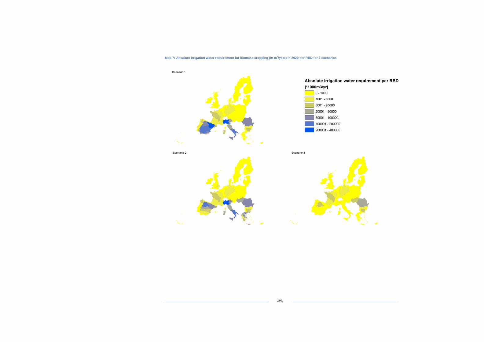
Map 7: Absolute irrigation water requirement for biomass cropping (in m3/year) in 2020 per RBD for 3 scenarios

-35-

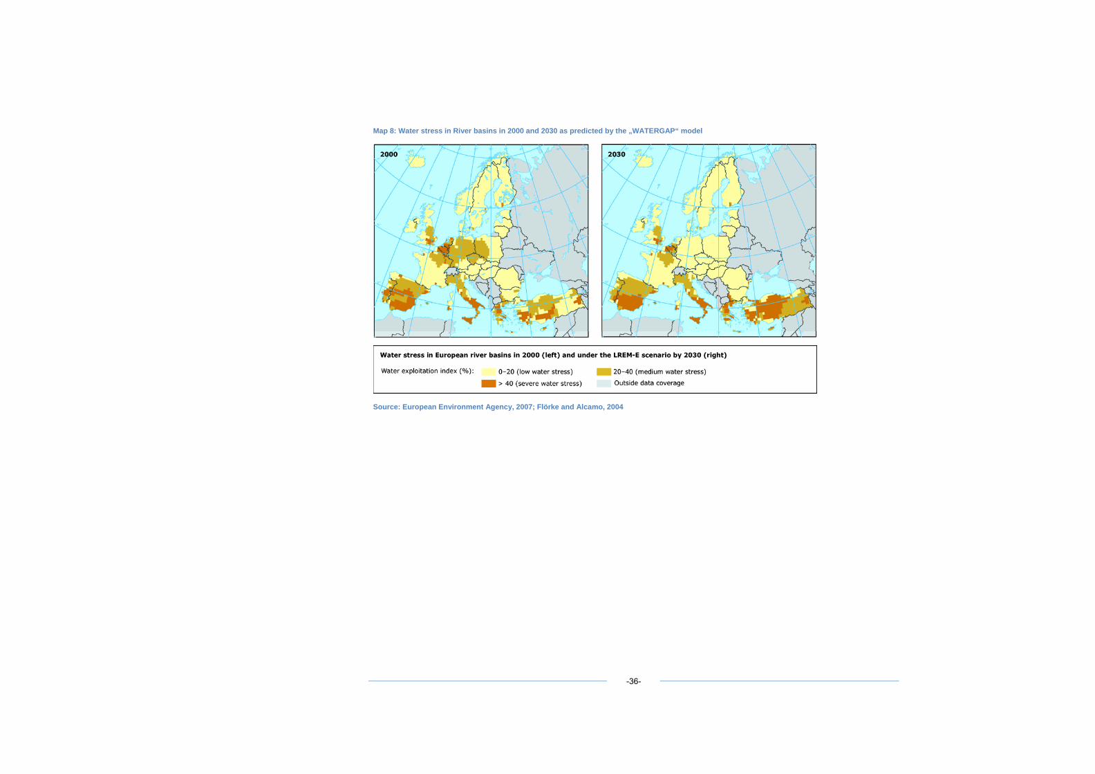
Map 8: Water stress in River basins in 2000 and 2030 as predicted by the „WATERGAP“ model

Source: European Environment Agency, 2007; Flörke and Alcamo, 2004

-36-

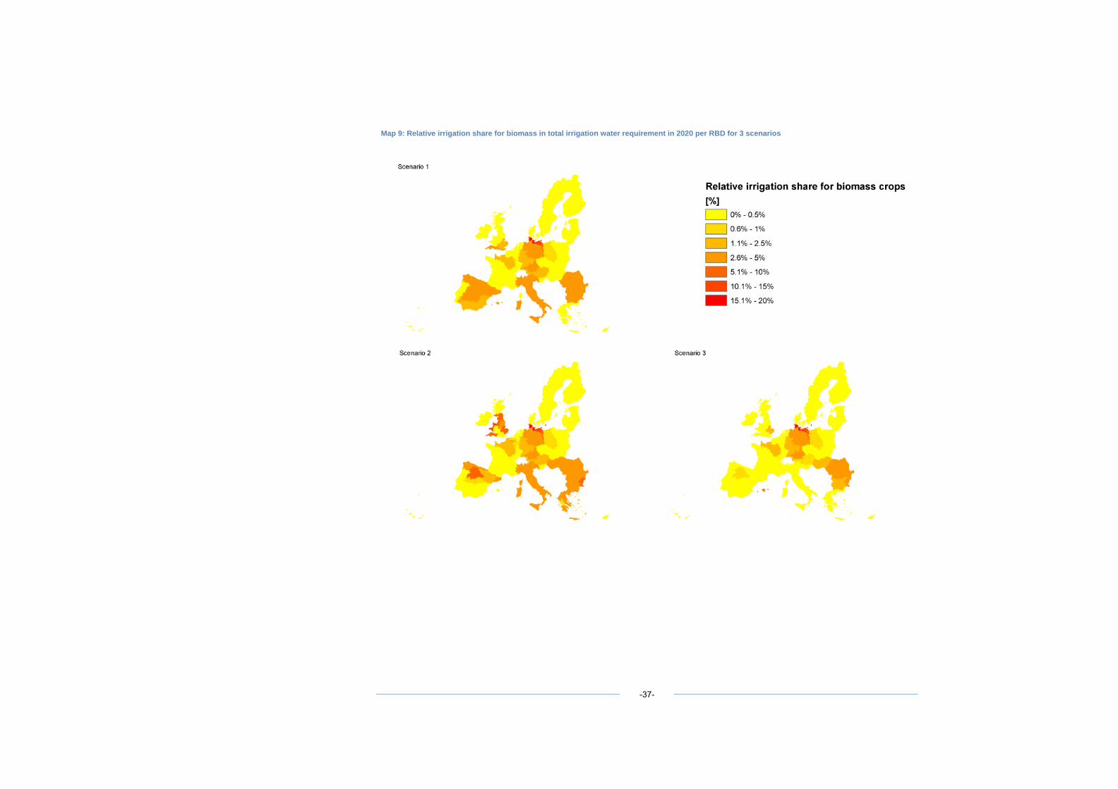
Map 9: Relative irrigation share for biomass in total irrigation water requirement in 2020 per RBD for 3 scenarios

-37-

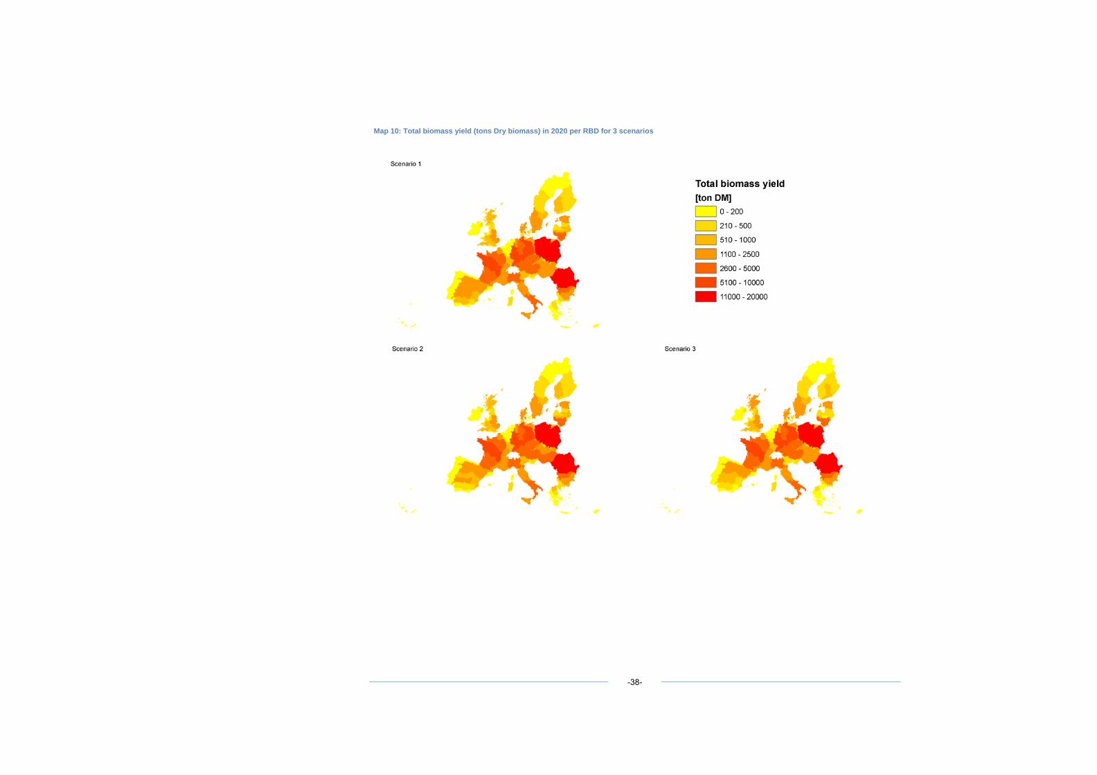
-38-

Map 10: Total biomass yield (tons Dry biomass) in 2020 per RBD for 3 scenarios

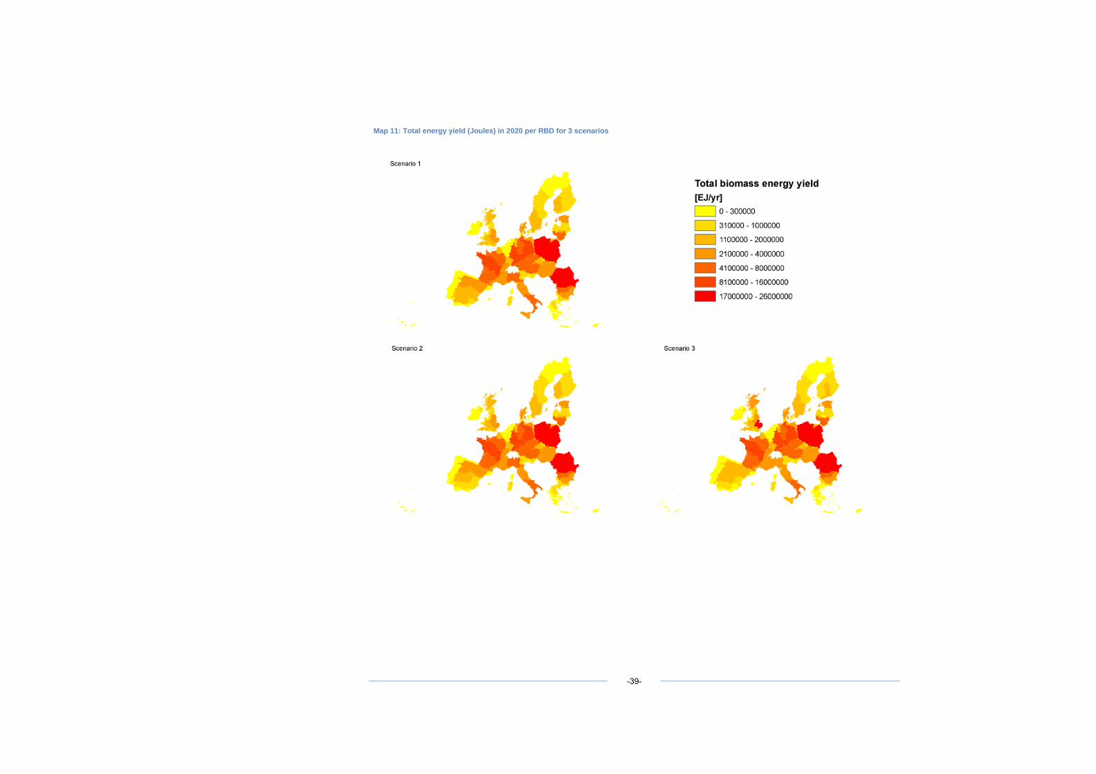
Map 11: Total energy yield (Joules) in 2020 per RBD for 3 scenarios

-39-

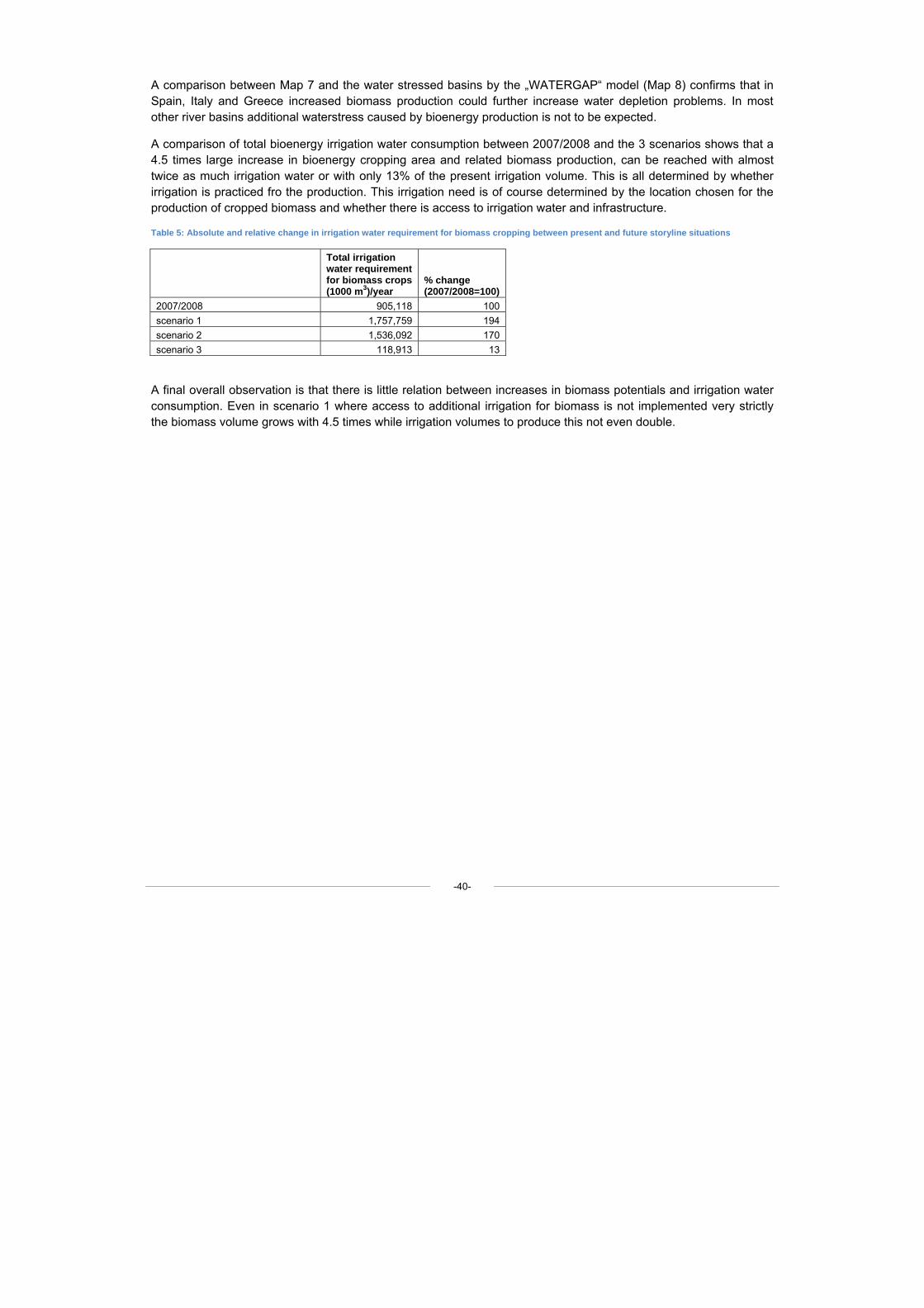
-40-

A comparison between Map 7 and the water stressed basins by the „WATERGAP“ model (Map 8) confirms that in Spain, Italy and Greece increased biomass production could further increase water depletion problems. In most other river basins additional waterstress caused by bioenergy production is not to be expected.

A comparison of total bioenergy irrigation water consumption between 2007/2008 and the 3 scenarios shows that a 4.5 times large increase in bioenergy cropping area and related biomass production, can be reached with almost twice as much irrigation water or with only 13% of the present irrigation volume. This is all determined by whether irrigation is practiced fro the production. This irrigation need is of course determined by the location chosen for the production of cropped biomass and whether there is access to irrigation water and infrastructure.

Table 5: Absolute and relative change in irrigation water requirement for biomass cropping between present and future storyline situations


% change (2007/2008=100)

2007/2008 905,118 100 scenario 1 1,757,759 194 scenario 2 1,536,092 170 scenario 3 118,913 13

A final overall observation is that there is little relation between increases in biomass potentials and irrigation water consumption. Even in scenario 1 where access to additional irrigation for biomass is not implemented very strictly the biomass volume grows with 4.5 times while irrigation volumes to produce this not even double.

-41-

7 Bioenergy in the context of current river basin planning

MS are currently in the process of drawing river basin management plans, including summaries of programmes of measures, in order to reach the main goal of “good status” of all waters.

In these plans also future water demand should be considered by MS. Annex III of the WFD it is states that: “The economic analysis shall contain enough information in sufficient detail (…) to take into account of long term forecasts of supply and demand for water in the RBD”. The increasing bioenergy demand is likely to influence this future demand and it is important to be aware of such changes in order to reduce the risk of water scarcity, but also to meet the

In the light of this study it was also an objective to assess to which extend bioenergy cropping is considered by MS in accordance with Annex III and as a risk for not achieving the good quantitative status.

In a first step the Art. 5 reports from 2003/2004 where used for this exercise. However it should be noted that an in-depth assessment for all Member Stated was not possible with the time and the resources given. So only those countries having already a high share in bioenergy cropping and those countries which are currently discussing a significant boost of their bioenergy activities were assessed16. From this assessment the following picture can be drawn:

• Some effort was done by the MS on the issue of forecasts, probably linked to the fact that this point is explicitly mentioned in the Annex III of the WFD. Only few MS did not provide any information on these issues (DK, LT, SI, SK, BUL (but that country provided some general information on future water supply for the Danube roof report), LU and BE (that both also did not provide information at the national level but contributed to the international basin roof reports)), while in some others only the issue of future water demand was mentioned but not of future water supply (e.g. EE, ESP).

• The work on this issue carried out by the MS mainly focuses on domestic (and partly also for industry) supply and demand. Bioenergy as part of agriculture where not addressed. Only for AUT, CZ and HU, where forecasts for water supply in four categories (households, industry without cooling water, industrial cooling water and agriculture) and total water demand including water losses by 2015 where provided.

In a second step the reports on the significant water management issues required under Art. 14. WFD where assessed. These reports are building beside other issues a basis for the development of the River Basin Management Plans. From the assessment it came clear that agriculture plays the most predominant role (Kampa et al., 2009). As shown in Figure 2 water abstraction for irrigation is the second most significant pressure reported by the MS in their draft River Basin Management Plans as regards to water quantity.

16 Germany, France, Austria, Spain, Romania, Bulgaria, Poland, Baltic States, Northern Countries.

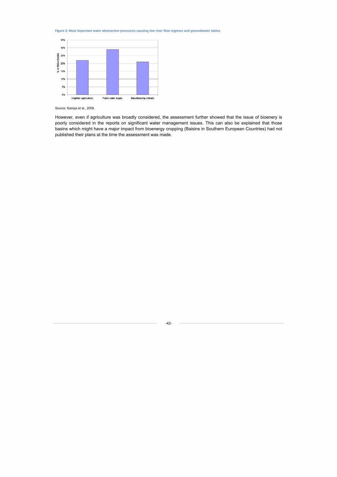
Figure 2: Most important water abstraction pressures causing low river flow regimes and groundwater tables

Source: Kampa et al., 2009.

However, even if agriculture was broadly considered, the assessment further showed that the issue of bioenery is poorly considered in the reports on significant water management issues. This can also be explained that those basins which might have a major impact from bioenergy cropping (Baisins in Southern European Countries) had not published their plans at the time the assessment was made.

-42-

-43-

8 Conclusion and recommendations

The future of bioenergy cropping and the achievement of the agreed bioenergy targets will strongly depend on water availability, and farming has significant impacts in terms of water quality and quantity (related to irrigation). Over-abstraction remains an issue and effective land-use planning needs to be ensured at appropriate levels. Particular attention in the case of water quantity needs to be paid to river basins facing quasi-permanent water stress or scarcity. This study analysed the potential impacts from bioenergy cropping on water quantity issues. It assessed the current situation and developed three storylines of potential developments.

While the current situation shows only a limited impact of bioenergy on water consumption this might change in the future depending on how policies will increase or decrease irrigation. The main conclusion from this scenario exercise can be summarised as follows:

• Stricter restrictions on water use in water scarce regions of the EU will not significantly influence the potential of the EU to produce large quantities of biomass. The potential biomass production is much more influenced by the amount of land to become available for biomass cropping then by the availability of irrigation water. This of course does not apply to all RBD regions in the EU, but for all basins outside the Mediterranean this is certainly the case. Stricter implementation of the Water Framework Directive in the South will therefore have consequences for the capacity of these countries to reach the biofuel targets, but it will certainly have positive influence on the environment under increased water demand for biomass cropping.

• A significant increase in biomass production in the EU will not need to increase the total irrigation water consumption. Stricter water use restrictions are only needed in the most water scarce regions to reach this low additional pressure on water resources for biomass cropping.

• In order to reach the bioenergy targets by 2020 it is most efficient therefore to stimulate the cropping of biomass in the Northern and central parts of Europe then in the South. The taking into use of additional land and efficient production techniques are more critical in reaching the targets then access to irrigation water.

• Placing the above made conclusions also in the context of future water consumption patterns as predicted by the „WATERGAP“ model (Flörke and Alcamo, 2004), an estimate of the potential future contribution of bioenergy to the total water withdrawals in a region can be made. Since according to the „WATERGAP“ predictions water withdrawals in Southern Europe and in the EU Candidate States are currently dominated by agricultural water use, and this will remain the same in the future, the contribution to biomass irrigation water consumption could then become more important. Combined with our results we can therefore conclude that in Southern Europe (France, Greece, Italy, Portugal and Spain) increased biomass cropping can be responsible for extra water abstraction problems. In Table 6 the bioenergy irrigation abstraction results are combined with the „WATERGAP“ 2030 baseline predictions on water shares of the total agricultural sector and total water withdrawals in the South of Europe in order to estimate bioenergy’s contribution to total water withdrawals.

It shows that in scenario 1, with no strict limits on use of water savings, bioenergy could contribute with 2.6% to the agricultural water abstraction level and with 1.4% to the total water abstraction. Stricter water abstraction measures for bioenergy could therefore have some effect but remain in the range of 1% to 3% of total water withdrawals.

Table 6: Bioenergy contribution to total water withdrawals in 2030 (Southern Europe*)

Bioenergy water use (1000 m3)/year)

% agriculture of total water abstraction

contribution bioenergy to total water abstraction

-44-

Scenario 1 1,757,759 2.6% 1.4% Scenario 2 1,536,092 2.2% 1.2% Scenario 3 118,913 0.2% 0.1% „WATERGAP“* 2030 agricultural water use = 68,344,000 in 1,000 m3

„WATERGAP“* 2030 total water withdrawals = 126,833,000 in 1,000 m3

*Includes France, Spain, Greece, Italy and Portugal

In order to reduce the pressure in these areas alternative water supply options like wastewater reuse could be considered as potential solutions. Theoretically, nutrients in domestic wastewater and organic waste are almost sufficient to fertilise crops, which would reduce fertilizer and fresh water needs. Human health considerations, which often block the use of wastewater in the agriculture sector, are not relevant for bioenergy production.

• In all other European regions this level will certainly be much lower given the outcomes of our scenario prediction that water abstraction rates are much lower for bioenergy and agricultural water abstraction in general is much lower for these regions. In increase in irrigated bioenergy cropping could therefore considered if WFD objectives are still met. This refers to water quality (see Annex 8) as well as water quantity.

-45-

9 Bibliography

Aden, A. (2007): Water Usage for Current and Future Ethanol Production. Southwest Hydrology September – October 2007, available at: www.swhydro.arizona.edu/archive/V6_N5/feature4.pdf.

Allen, R.G., L.S. Pereira, D. Raes and M. Smith (1998): Crop evapotranspiration: guidelines for computing crop water requirements. Irrigation and Drainage Paper nr. 56. FAO, Rome, Italy, 300 pp.

Barz, M.; Ahlhaus, M. (2005): Use of Bioenergy in the Baltic Sea Regions. Conference Proceedings. 2nd International Baltic Bioenergy Conference. Bioenergy Conference, Stralsund, available at: http://www.fh-stralsund.de/dokumentenverwaltung/dokumanagement/psfile/file/48/Proceeding457544033413a.pdf.

Berndes, G. (2002): Bioenergy and water – the implications of large-scale bioenergy production for water use and supply. Global Environmental Change 12 (4): 253-271.

Bioheritage (2008): The future of European semi‐natural grasslands. Workshop report 20/21 October 2008, Konstanz.

Boons-Prins, E.R., G.H.J. de Koning, C.A. van Diepen, F.W.T. Penning de Vries. (1993): Crop specific simulation parameters for yield forecasting across the European Community. Simulation Reports CABO-TT 32. 43 pp and 123 pp Annexes.

Brainbows Informationsmanagement GmbH (2007): Biomasse-Ressourcenpotenzial in Österreich -Studie im Auftrag der RENERGIE Raiffeisen Managementgesellschaft für erneuerbare Energie GmbH. Endbericht, 07.05.2007.

Bruton, T.; McDermott, R. (2006): Bioenergy industry sets targets for future, available at: http://www.farmersjournal.ie/2006/0128/farmmanagement/crops/index.shtml.

Chang, M. (2006). Forest Hydrology: An Introduction to Water and Forests, 2nd Ed. London: Taylor & Francis.

Christou, M.; Fernandez, J.; Gosse, G.; Venturi, G.; Bridgwater, A.; Scheurlen, K.; Obernberger, I.; Van de Beld, L.; Soldatos, P.; Reinhardt, G. (2004): Bioenergy Chains from Perennial Crops in South Europe. In Proc. of the 2nd World Conference and Exhibitions on Biomass, Rom.

Committee on Water Implications of Biofuels Production in the United States, National Research Council (2008): Water Implications of Biofuels Production in the United States, available at: http://www.nap.edu/catalog.php?record_id=12039#toc.

Cosentino, S.L., Patanè, C., Sanzone, E., Copani, V., Foti, S., (2007): Effects of soil water content and nitrogen supply on the productivity of Miscanthus x giganteus Greef et Deu. in a Mediterranean environment. Industrial Crops and Products 25 (207), 75-88.

Diepen, C.A. van, Wolf, J., Keulen, H. van (1989): WOFOST: a simulation model of crop production. Soil Use and Management, 5:16-24.

Dirksen, W.; Huppert, W. (eds.) (2006): Irrigation Sector Reform in Central and Eastern European Countries. GTZ (Deutsche Gesellschaft für Technische Zusammenarbeit), Eschborn, ICID, New Delhi.

Doorenbos, J. and A.H. Kassam (1979): Yield response to water. Irrigation and Drainage. Paper nr. 33. FAO, Rome, Italy, 193 pp.

Doran, M. (2008): TS 4E – The Surveyors Role in Promoting Sustainability and the Use of Sustainable Resources. Contribution of Energy Crops in Displacing Fossil Fuels in the EU Integrating Generations. FIG Working Week 2008. Stockholm, Sweden 14-19 June 2008, available at: http://www.fig.net/pub/fig2008/papers/ts04e/ts04e_02_doran_3082.pdf.

http://www.swhydro.arizona.edu/archive/V6_N5/feature4.pdf

http://www.fh-stralsund.de/dokumentenverwaltung/dokumanagement/psfile/file/48/Proceeding457544033413a.pdf

http://www.fh-stralsund.de/dokumentenverwaltung/dokumanagement/psfile/file/48/Proceeding457544033413a.pdf

http://www.fig.net/pub/fig2008/papers/ts04e/ts04e_02_doran_3082.pdf

-46-

Dworak, T.; Eppler, U.; Petersen, J.E.; Schlegel, S.; Laaser, C. (2008): A review of the possible impact of biomass production from agriculture on water.

Dworak, T.; Strosser, P.; Joyce, J. (unpublished): Scenarios of water demand management – Impacts at regional level.

Edwards, R.; Larive, J-F; Mahieu, V.; Rouveirolles, P.; (2007): Well-to-wheels analysis of future automotive fuels and power trains in the European context. Commissioned by JRC, Eucar and Concawe.

European Commission (2002): European Agriculture entering the 21st century. Directorate General Agriculture; Brussels, October, 2002.

European Commission (2004): Prospects for agricultural markets. Directorate General Agriculture; Brussels, July, 2004.

European Commission (2006a): Water Scarcity and Drought, In-depth assessment, First interim report.

European Commission (2006b): Water scarcity Management in the context of the WFD, Policy Summary.

European Commission (2009): Regions 2020 – The climate change challenge for European regions, available at: http://ec.europa.eu/regional_policy/sources/docoffic/working/regions2020/pdf/regions2020_climat.pdf.

European Council (1979): Council Directive 79/409/EEC of 2 April 1979 on the conservation of wild birds.

European Council (1979): Council Directive 80/68/EEC of 17 December 1979 on the protection of groundwater against pollution caused by certain dangerous substances.

European Council (1986): Council Directive 86/278/EEC of 12 June 1986 on the protection of the environment, and in particular of the soil, when sewage sludge is used in agriculture.

European Council (1991): Council Directive 91/676/EEC of 12 December 1991 concerning the protection of waters against pollution caused by nitrates from agricultural sources.

European Council (1992): Council Directive 92/43/EEC of 21 May 1992 on the conservation of natural habitats and of wild fauna and flora.

European Council (2003): Council Regulation (EC) No 1782/2003 of 29 September 2003 establishing common rules for direct support schemes under the common agricultural policy and establishing certain support schemes for farmers.

European Council (2009): Council Regulation (EC) No 73/2009 of 19 January 2009 establishing common rules for direct support schemes for farmers under the common agricultural policy and establishing certain support schemes for farmers, amending Regulations (EC) No 1290/2005, (EC) No 247/2006, (EC) No 378/2007 and repealing Regulation (EC) No 1782/2003.

European Environment Agency (2007): Estimating the environmentally compatible bio-energy potential from agriculture, EEA technical Report 12/2007. Copenhagen: EEA, available at http://reports.eea.europa.eu/technical_report_2007_12/en.

European Parliament and of the Council (2000): Directive 2000/60/EC of 22 December 2000 establishing a framework for the Community action in the field of water policy.

European Parliament and of the Council (2009): Directive 2009/28/EC of 23 April 2009 on the promotion of the use of energy from renewable sources and amending and subsequently repealing Directives 2001/77/EC and 2003/30/EC.

http://ec.europa.eu/regional_policy/sources/docoffic/working/regions2020/pdf/regions2020_climat.pdf

http://reports.eea.europa.eu/technical_report_2007_12/en

-47-

Flörke, M.; Alcamo, J. (2004): European outlook on water use. Final report, Center for Environmental Systems Research, Kassel. Garofalo, R. (2007): Biodiesel Chains: Promoting favourable conditions to establish biodiesel market actions. WP 2 “Biodiesel market status”. Deliverable 7: EU-27 Biodiesel Report.

Gray, K.; Zhao, L.; Emptage, M. (2006): Biothanol. Current Opinion in Chemical Biology 10 (2): 141–146.

Hénard, M.-C.; Audran, X. (2007): France Bio-Fuels – French Biofuel Production Plans 2007, available at: http://www.fas.usda.gov/gainfiles/200701/146279894.pdf.

Iglesias A; Avis, K.; Benzie, M.; Fisher, P.; Harley, M.; Hodgson, N.; Horrocks, L., Moneo, M.; Webb, J. (2007): Adaptation to Climate Change in the Agricultural Sector. Report to European Commission Directorate - General for Agriculture and Rural Development.

International Energy Agency (2008): From 1st to 2nd-Generation Biofuel Technologies – An overview of current industry and RD&D activities.

Johnson, F. X.; Roman, M. (2008): Biofuels sustainability criteria: Relevant issues to the proposed Directive on the promotion of the use of energy from renewable sources. Consolidated study (IP/A/ ENVI/IC/2008-051), prepared for the European Parliament: Policy Department Economic and Scientific Policy, Brussels.

Joint Research Centre of the EU, European Environmental Agency (2006): Proceedings of an expert meeting on energy crops in the Mediterranean; Madrid.

Kampa, E.; Dworak, T.; Grandmougin,B.; Cheung-Ah-Seung, E.; Mattheiß, V.; Strosser, P., Campling, P. (2009): Active Involvement in River basin Management – Plunge into the debate, Conference document for the 2nd European Water Conference, 2-3 April 2009, Brussels.

Keeney, D.; Müller, M. (2006): Water use by Ethanol Plants: Potential Challenges. Minnesota: Institute for Agriculture and Trade Policy, available at: www.agobservatory.org/library.cfm?refid=89449.

Keulen, H. van, Wolf J. (Eds) (1986): Modelling of agricultural production: weather, soils and crops. Simulation Monographs, Pudoc Wageningen, The Netherlands.

Kondilia, E. M.; Kaldellis, J. K. (2007): Biofuel implementation in East Europe: Current status and future prospects. Renewable and Sustainable Energy Reviews 11: 2137–2151.

Leppiman, A. (2005): Current status of bioenergy and future prospects in Baltic Sea Area, available at: http://www.nordicinnovation.net/_img/leppiman.pdf.

Lewandowski, I., Scurlock, J.M.O., Lindvall, E., Christou, M., (2003): The development and current status of perennial rhizomatous grasses as energy crops in the US and Europe. Biomass and Bioenergy 25 (2003), 335 – 361.

Lind, O. T.; Davalos-Lind, L. (2002): Interaction of water quantity with water quality: The Lake Chapala example. Advances in Mexican Limnology: Basic and Applied Aspects. Special Issue. Hydrobiologia. Kluwer Academic/Plenum Publishers. 467:159-167.

Nilsson, C.; Malm-Renöfält, B. (2008): Linking flow regime and water quality in rivers: a challenge to adaptive catchment management. Ecology and Society 13 (2), available at: http://www.ecologyandsociety.org/vol13/iss2/art18/.

Panoutsou, C. (2008): Bioenergy in Greece: Policies, diffusion framework and stakeholder interactions. Energy Policy 36 (10): 3674-3685.

Pate, R.; Hightower, M.; Cameron, C.; Einfeld, W. (2007.): Overview of Energy-Water Interdependencies and the Emerging Energy Demands on Water Resources. Report SAND 2007-1249C. Las Alamos, NM: Sandia National Laboratories in National Academy of Sciences.

http://www.agobservatory.org/library.cfm?refid=89449

http://www.nordicinnovation.net/_img/leppiman.pdf

http://www.ecologyandsociety.org/vol13/iss2/art18/

-48-

Perini, S. (2007): Italy – Trade Policy Monitoring – Biofuels 2007, available at: http://www.fas.usda.gov/gainfiles/200704/146280702.pdf.

Raab (2007): Presentation on Bioenergie vom Acker – Potenziale in Österreich und in der erweiterten EU, at the Wintertagung 2007, 13. Februar 2007.

Schröter, D.; Acosta-Michlik, L.; Arnell, A. W.; Araújo, M. B.; Badeck, F.; Bakker, M.; Bondeau, A.; Bugmann, H.; Carter, T.; de la Vega-Leinert, A. C.; Erhard, M.; Espiñeira, G. Z.; Ewert, F.; Fritsch, U.; Friedlingstein, P.; Glendining, M.; Gracia, C. A.; Hickler, T.; House, J.; Hulme, M.; Kankaanpää, S.; Klein, R. J. T.; Krukenberg, B.; Lavorel, S.; Leemans, R.; Lindner, M.; Liski, J.; Metzger, M. J.; Meyer, J.; Mitchell, T.; Mohren, F.; Morales, P.; Moreno, M. J.; Reginster, I.; Reidsma, P.; Rounsevell, M.; Pla, E.; Pluimers, J.; Prentice, I. C.; Pussinen, A.; Sánchez, A.; Sabaté, S.; Sitch, S.; Smith, B.; Smith, J.; Smith, P.; Sykes, M. T.; Thonicke, K.; Thuiller, W.; Tuck, G.; van der Werf, G.; Vayreda, J.; Wattenbach, M.; Wilson, D. W.; Woodward, F. I.; Zaehle, S.; Zierl, B.; Zudin, S.; Cramer, W. (2004): Advanced Terrestrial Ecosystem Analysis and Modeling (ATEAM). Final report 2004, available at http://www.pik-potsdam.de/ateam/ateam_final_report_sections_5_to_6.pdf.

Supit, I., Hooijer, A.A., Diepen, C.A. van, (Eds.) (1994): System description of the WOFOST 6.0 crop simulation model implemented in CGMS. Publication EUR 15956 EN of the Office for Official Publications of the EU, Luxembourg.

Tilman, D.; Hill, J.; Lehman, C.: (2006): Carbon-Negative Biofuels from Low-Input High-Diversity Grassland Biomass. Science 314 (5805): 1598-1600.

Tuck, G.; Glendining, M. J.; Smith, P.; House, J. I.; Wattenbach, M. (2006): The potential distribution of bioenergy crops in Europe under present and future climate. Biomass and Bioenergy 30 (3): 183-197.

Vossen, P., Rijks, D.A. (1995):. Early crop yield assessment of the EU countries. The system implemented by the Joint Research Centre. Publication EUR 16318 EN of the Office for Official Publications of the EU, Luxembourg.

Wesolowski, J. (2005): Sources of energy from agricultural crops in Poland, available at: http://www.agri.ee/public/juurkataloog/BIOENERGEETIKA/Wesolowski.ppt

Wriedt, G.; van der Velde, M.; Aloe, A.; Bouraoui, F. (2008): Water Requirements for Irrigation in the European Union. EUR Scientific and Technical Research Series. European Commission, Joint Research Centre, Ispra.

-49-

Annex 1: Detailed description of the methods used to estimate water requirements and yield level for biomass cropping in the present and future situation

1. Defining the state of the art in crop growth modelling and crop water requirements The most widely applied and therefore classical method of estimating crop water use and related crop yield is the “crop yield response to water procedure” described in by the FAO (Doorenbos and Kassam, 1979). The approach is based on the quantification of the cumulative crop evapotranspiration during the crop growing season.

The maximum evapotranspiration is the water requirement for the crop, defined as:

ETm = Kc x ET0

Where:

Kc: crop coefficient according to Doorenbos and Pruitt

ET0: potential Evaporation and Transpiration in mm/day or mm/decade according to Penman-Monteith

This maximum evapotranspiration rate ETm is realized when the root zone is well watered and the soil surface wet. The value of the Kc coefficients depends on crop type and canopy cover. When water supply to the crop roots is insufficient, the actual evapotranspiration ETa is reduced, and a water deficit develops in the crop, often called crop water stress, whereby the growth of the crop will be reduced proportionally.

As reference yield linked to maximum evapotranspiration is used the maximum yield Ym achievable in a given climate under ideal, constraint-free conditions, i.e. assuming perfect management of water and fertilizer and control of pests and diseases. The actual yield of a field crop or tree crop Ya affected by drought stress can be quantified by relating the relative yield loss to relative reduction in evapotranspiration using the following equation:

(Ym-Ya)/Ym = Ky (ETm-ETa)/ETm

Often also written as:

1 – (Ya / Ym) = Ky (1 – [ETa / ETm])

Where:

Ym and Ya are the maximum and actual yield, ETm and ETa are the maximum and actual evapotranspiration, and Ky is the proportionality factor between relative yield loss and relative reduction in evapotranspiration.

While the evapotranspiration for a given crop field is calculated on the basis of daily (or 10-daily) weather data and an assumed crop canopy curve (LAI curve) , the maximum yield is estimated directly on the basis of crop field trials or farm surveys. Crop yield can also be modeled by assuming that the accumulated biomass is directly related to the amount of crop evapotranspiration. The proportionality factor is the water use efficiency (WUE), which can be taken from literature. Similarly a fixed harvest index can be chosen to determine the yield as useful fraction of the total crop biomass. Alternatively, it is also possible to quantify the biomass using a crop simulation model, which takes into account the basic physiological crop growth processes such as photosynthesis, respiration, growth and decay of leaves and other plant organs and crop phenology.

The calculation procedure is valid for a homogeneous crop field. For application at the scale of a farm, region, country or continent the agricultural area is subdivided in calculation units, defined by crop type, crop calendar, weather and soil conditions, possibly split by management level, and into irrigated and rainfed areas.

-50-

The original crop response procedure is a water-driven crop model that requires a relatively low number of parameters and input data to estimate the yield response to water of the major field crops

The “crop yield response to water procedure” has been applied for the assessment of both irrigation requirements and of crop yield reduction due to drought.

The method is consistent, simple and robust and therefore attractive. However, its simplicity and its reliance on empirical and partly intuitive parameters form also particular limitations of the method. For specific applications refinements in the modeling procedures have been developed over the years, both in the calculation of the crop water balance and of the development and growth of the crop.

The FAO Water Satisfaction Index (WSI)

The FAO CSWB or CSSWB (Crop Specific (Soil) Water Balance) was first published in 1986 by FAO with examples from semi-arid tropical climates. The main output of CSWB was the Water Requirement Satisfaction Index (WRSI or WSI). Since then the index has become the most widely used crop yield indicator for the assessment of yield reduction due to drought, all over the world. At the same time many variants of the calculation procedure, model coefficients, and of data standards have been developed, which are being applied at local to global scales. The index is a qualitative index, expressed as a percentage of maximum yield, which can be used independently, or combined with other models, such as FAO’s crop yield functions according to FAO’s yield response to water stress. In addition, the CWSB method requires the calculation of the soil water storage, and evapotranspiration deficit, and provides an estimate of duration that the soil has been dry, which themselves can be used as qualitative indicators of the outcome of the regional cropping season.

The Global WSI model (GWSI) developed by JRC Agri4Cast is based on the FAO-CWSB method and applied to the whole world with a resolution of 1x1 degree climatic grid cells, which are subdivided into smaller agricultural land areas (0.1x0.1 degrees) .GWSI contains a simple soil water balance model which is used to assess the impact of weather conditions on crops. The water balance of the specific crop is calculated in time increments: decades (10-days). The equation of the water balance is:

Wt = Wt-1 + R – ETm

Where:

Wt: amount of available water stored in the soil at the end of a dekad (t).

Wt-1: amount of available water stored in the soil at the end of the previous dekad (t-1).

R: cumulated rainfall during the dekad (mm/dekad).

ETm: cumulated maximum evapotranspiration during the dekad for a given crop (mm/dekad) defined as: ETm = Kc x ET0

The soil profile functions as a water reservoir, like a bucket. When (Rain - ETm) exceeds the storage capacity, the excess rainfall is accounted for as water surplus or deep percolation. Run-off is not taken into account because 1 by 1 degree is too coarse to account for local run-off and run-on which average each other out. It is assumed that all rainfall is effective. The storage capacity of the soil profile is the amount of water between field capacity and wilting point taken for the whole rooting depth.

The water surplus (deep percolation) is defined as follows:

IF Wt > StorageCapacity: WaterSurplus = Wt - StorageCapacity

If Wt becomes less than 0 the soil has a severe water deficit, D. This is an important variable to calculate the WSI.

IF Wt < 0: D = Wt

At the end of the calculation time step Wt is reset between the limits 0 and Storage capacity.

The output variables of GWSI at the end of the growing season are cumulated values (since planting date) for Water Satisfaction Index (WSI), Water Deficit (D), Water Surplus (WS), ETa , Rainfall, Yield (on regional level).

As reference the long term average of these indicators is used, based on the 15 most recent and complete years.

The WSI is a qualitative index expressing to which percentage the crop water requirements have been met. It is calculated on the basis of 10-daily values of D, by summing the values of D and dividing this sum by the total seasonal water requirement of the plant:

⎟⎟⎟⎟⎟

⎠

⎞

⎟⎠

⎞

⎟⎠

⎞|

⎜⎜⎜⎜⎜

⎝

⎛

⎜⎝

⎛

⎜⎝

⎛

−∗=

∑

∑

=

=n

d

n

d

WR

DWSI

1

1|

1100

Where:

D = Soil water deficit (mm/dekad)

WR = Maximum plant water requirement or ETm (mm/dekad)

d = dekad

n = harvest dekad

The WSI decreases when water stress is experienced. From the equation it can be understood that the decrease in WSI is highest when the severity of D is high, and when the growth cycle (thus sum of ETm) is short.

An attractive option that is sometimes applied is to extend the FAO-CSWB model from a soil water model into a crop yield model by applying the ratio ETa/ETm in a crop yield function. Such as used in the FAO crop yield response model of Doorenbos and Kassam (1979). The ratio [ETa / ETm] can be replaced by the WSI value, which leads to the same results.

The “crop yield response to water procedure” is updated recently in the Aquastat model (Raes et al., 2009). Important improvements are the separation of the ET into soil evaporation (E) and crop transpiration (Tr) and the distinction between final yield (Y), biomass (B) and harvest index (HI). The splitting of ET makes the non-productive consumptive use of water (E) visible, especially relevant before canopy closure.

The new Acquastat model offers more detail in the modeling of the soil-plant-atmosphere continuum. The new components include the soil water balance; and a crop model. The crop model simulates the plant dynamics during the growth cycle in terms of phenology, aerial canopy, rooting depth, biomass production and harvestable yield. Additionally, some management aspects are explicitly considered (e.g. irrigation, fertilization, etc.), as they will affect the soil water balance, crop development and therefore final yield.

The WOFOST model

Apart from water-driven crop models developed by FAO a number of crop models have been developed by the school of CT de Wit since the 1960’s with the aim to determine the upper limits of production, as determined by

-51-

-52-

climatic conditions and the genetic potential of the crop. These models are based on a number of crop physiological responses to weather and soil conditions. This has resulted in a family of crop growth models, of which SUCROS, WOFOST and ORYZA are the best known members.

These models are used to explain or predict the potential and attainable yields of crops under the environmental and management conditions, and to compare these yields against actual yields in a field, farm, or a region, to quantify the yield gap and to identify the constraints limiting crop production. The WOFOST model is the weather driven crop engine of the Crop Growth Monitoring System (CGMS) of the JRC-Agri4Cast action.

The principles of the WOFOST crop growth simulation model have been discussed by van Keulen and Wolf (1986) and van Diepen et al. (1989). Its implementation in CGMS and its structure is described by Supit et al. (1994), and its application by Vossen and Rijks (1995).

In WOFOST first, instantaneous photosynthesis, calculated at three depths in the canopy for three moments of the day, is integrated over the depth of the canopy and over the light period to arrive at daily total canopy photosynthesis. After subtracting maintenance respiration, assimilates are partitioned over roots, stems, leaves and grains as a function of the development stage, which is calculated by integrating the daily development rate, described as a function of temperature and photoperiod. Assimilates are then converted into structural plant material taking into account growth respiration. Leaf area growth is driven by temperature and limited by assimilate availability.

Above ground dry matter accumulation and its distribution over leaves, stems and grains on a hectare basis are simulated from sowing to maturity on the basis of physiological processes as determined by the crop’s response to daily weather: (rainfall, solar radiation, photoperiod, minimum and maximum temperature and air humidity), soil moisture status (i.e. Ta/Tp, alike the FAO models) and management practices (i.e. sowing density, planting date, etc.). Water supply to the roots, infiltration, runoff, percolation, capillary rise and redistribution of water in a one-dimensional profile are derived from hydraulic characteristics and moisture storage capacity of the soil.

Crop model parameters describing the specific growth potentials of individual crops are an essential input to any crop growth simulation model. Boons-Prins et al. (1993) constructed the first CGMS crop files for: winter wheat, spring wheat, barley rice, potato, sugar beet, field beans, soybean, rapeseed, sunflower on the basis of data from field trials executed in Belgium, United Kingdom and the Netherlands and the specific crop literature. These crop files contain basic information such as rooting depth, temperature threshold for growth, etc. Also included is detailed physiological information such as heat sums to reach various phonological stages, energy conversion, portioning of assimilates over various plant organs. For specific crop varieties grown in certain regions some parameters in the crop files have been modified. Since new crop varieties are constantly introduced, crop parameters that describe crop growth and development, such as for example the temperature sums to reach the flowering stage, are regularly updated and calibrated as new information comes available.

The need for soil data is twofold. Rooting depth and water retention characteristics determine the maximum available water that can be stored by the soil. Important system aspects like initial available water at the start of the growing season and the soil capacity to buffer infiltrated rainfall are influenced by these soil properties. Further, soil data are used to define whether a crop has to be included in the simulation for a given soil type. For instance shallow soil types are excluded as these soils are not be cropped in reality. The current CGMS is based on the Soil Geographical Database of Europe (SGDBE) version 4 covering pan Europe. The resolution available for geographical representation is 1:1,000,000 for most countries. The SGDBE contains list of Soil Typologic Units (STU), characterizing distinct soil types that have been identified and described. The STU are described by attributes specifying the nature and properties of the soils, for example texture, the moisture regime, the stoniness etc. Because it is not technically feasible to delineate each STU on the map, the STUs are grouped into Soil Mapping Units (SMU) to form soil associations..Soil attributes like rooting depth and water retention required in the

-53-

crop water model of CGMS have been derived from basic properties like soil name and texture applying so called pedotransfer rules.

CGMS-Europe contains a meteo data base with historic daily meteorological data from weather stations. For the EU15 and neighbouring countries data from approximately 380 stations with data since 1976 are available, in some cases back to 1930. Since about 1990 the data set was extended with stations from eastern Europe, western Russia, Maghreb and Turkey, while the station density increased over the entire area . Presently, data from nearly 7100 stations is available. Of these stations about 2500 receive daily meteorological information. The historic data were converted into consistent units and scanned for inconsistencies and non realistic values. Variables covered are global radiation, air temperature, dew-point temperature (humidity), pressure at sea level, wind speed, amounts of precipitation, clouds, and sunshine duration.

Although CGMS can be applied at station level, CGMS runs on a 50 by 50 km grid for the following reasons: irregular spatial distribution of the meteorological stations, spatial variability of the crop and land use, crop and soil information. The weather variables needed as input are: precipitation, minimum and maximum temperature, global radiation, wind speed and vapour pressure. The data interpolation is based on the averaging of values from weather stations surrounding a given grid cell, with a preference for a number of three similar stations, Similarity is expressed as a score based on distance between grid centre and station, difference in altitude and in distance to the coast, and position relative to a climatic barrier.

The interpolation is executed in two steps: first, from the list of suitable stations a set of stations is selected that is most suitable for the interpolation. Second, a simple average is calculated for most of the meteorological parameters, with a correction for the altitude difference between the station and grid cell centre in case of temperature and vapour pressure. As an exception rainfall data are taken directly from the most similar station. This empirical interpolation method is robust and accurate.

2. Further technical details on the model approach to estimating the current water needs of bioenergy crops To perform step 4 (see Chapter 4, Section 4.2), which is the determination of the present irrigation water requirements of bioenergy crops, the potential and water-limited yield and the amount of water directly used by the crops for transpiration under potential conditions have been extracted from the data base of the Crop Growth Monitoring System (CGMS) of the MARS project of the Joint Research Center. The data have been collected for six crops at NUTS-2 level. EU-29 has 258 NUTS-2 regions. The six crops are winter wheat, spring barley, grain maize, oil seed rape, sunflower and sugar beet17.

CGMS uses a grid cells of 50x50 km as basic climatic grid on which daily weather data are available as time series over many years. In this study the five-year period of 2003-2007 has been used as input for the simulation of crop growth and water use with CGMS. The simulations have been carried out for all regions where the agricultural statistics mention that the crop is grown. In addition to weather data the simulation model requires as input soil data and crop parameters for each given crop. The final simulated values of yield and water use at the end of the season have been averaged over the five years, and aggregated over NUTS-2 regions.

17 The water use requirements and rainfall deficiency could have also be determined from the Global Water Satisfaction Index (GWSI) system of JRC for the same crops of interest: Spring barley, grain maize, spring wheat, grain sorghum, soybean. However, the administrative subdivision of Europe applied in GWSI is based on FAO’s global administrative maps which does not correspond to the NUTS-2 level subdivision over Europe, and requires manual recoding. Since the CGMS provided data at NUTS-2 which were more easy to convert further to the River Basin Districts (RBD) boundaries we made a choice for the CGMS based modelling runs.

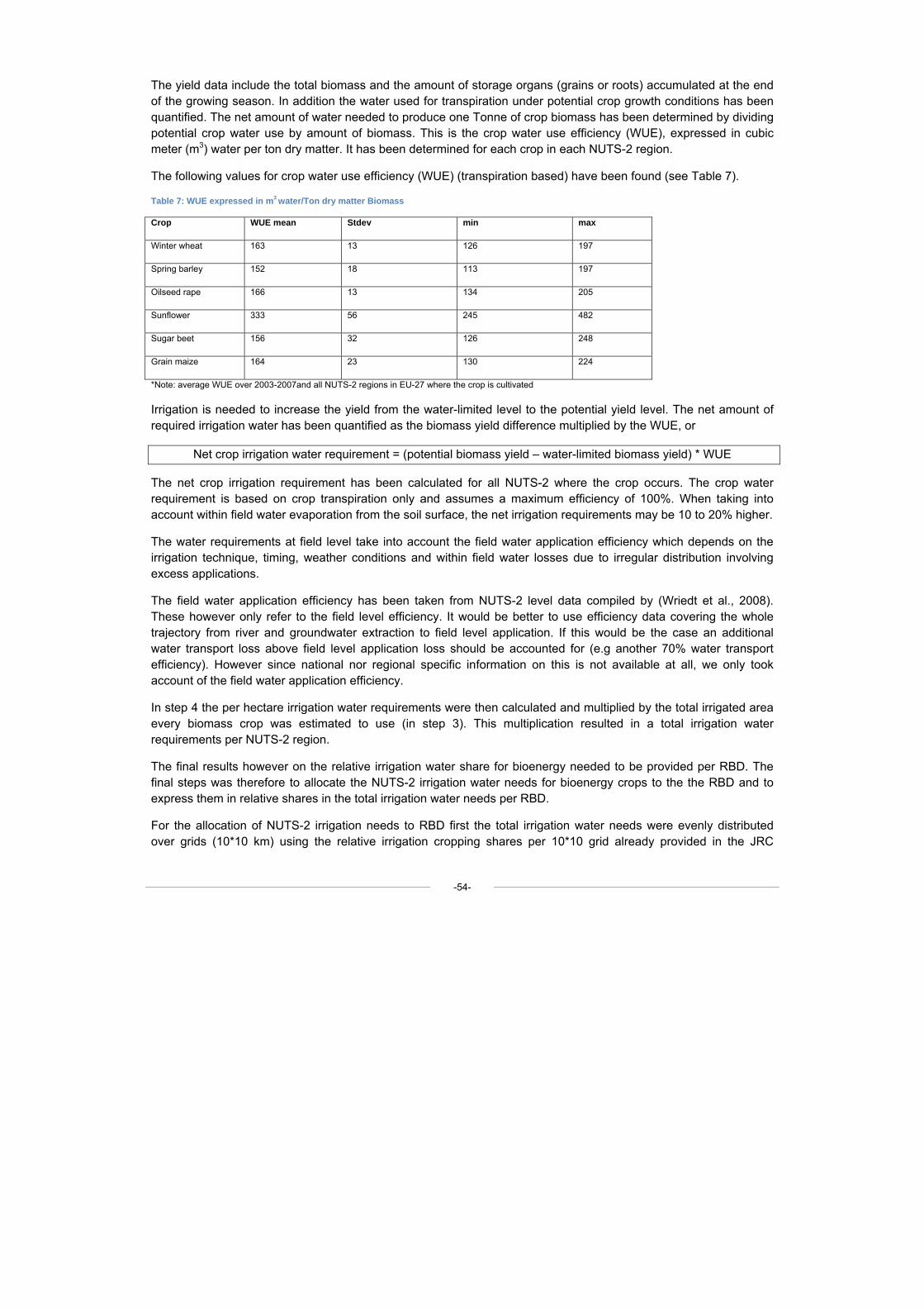
-54-

The yield data include the total biomass and the amount of storage organs (grains or roots) accumulated at the end of the growing season. In addition the water used for transpiration under potential crop growth conditions has been quantified. The net amount of water needed to produce one Tonne of crop biomass has been determined by dividing potential crop water use by amount of biomass. This is the crop water use efficiency (WUE), expressed in cubic meter (m3) water per ton dry matter. It has been determined for each crop in each NUTS-2 region.

The following values for crop water use efficiency (WUE) (transpiration based) have been found (see Table 7).

Table 7: WUE expressed in m3 water/Ton dry matter Biomass

Crop WUE mean Stdev min max

Winter wheat 163 13 126 197

Spring barley 152 18 113 197

Oilseed rape 166 13 134 205

Sunflower 333 56 245 482

Sugar beet 156 32 126 248

Grain maize 164 23 130 224

*Note: average WUE over 2003-2007and all NUTS-2 regions in EU-27 where the crop is cultivated

Irrigation is needed to increase the yield from the water-limited level to the potential yield level. The net amount of required irrigation water has been quantified as the biomass yield difference multiplied by the WUE, or

Net crop irrigation water requirement = (potential biomass yield – water-limited biomass yield) * WUE

The net crop irrigation requirement has been calculated for all NUTS-2 where the crop occurs. The crop water requirement is based on crop transpiration only and assumes a maximum efficiency of 100%. When taking into account within field water evaporation from the soil surface, the net irrigation requirements may be 10 to 20% higher.

The water requirements at field level take into account the field water application efficiency which depends on the irrigation technique, timing, weather conditions and within field water losses due to irregular distribution involving excess applications.

The field water application efficiency has been taken from NUTS-2 level data compiled by (Wriedt et al., 2008). These however only refer to the field level efficiency. It would be better to use efficiency data covering the whole trajectory from river and groundwater extraction to field level application. If this would be the case an additional water transport loss above field level application loss should be accounted for (e.g another 70% water transport efficiency). However since national nor regional specific information on this is not available at all, we only took account of the field water application efficiency.

In step 4 the per hectare irrigation water requirements were then calculated and multiplied by the total irrigated area every biomass crop was estimated to use (in step 3). This multiplication resulted in a total irrigation water requirements per NUTS-2 region.

The final results however on the relative irrigation water share for bioenergy needed to be provided per RBD. The final steps was therefore to allocate the NUTS-2 irrigation water needs for bioenergy crops to the the RBD and to express them in relative shares in the total irrigation water needs per RBD.

For the allocation of NUTS-2 irrigation needs to RBD first the total irrigation water needs were evenly distributed over grids (10*10 km) using the relative irrigation cropping shares per 10*10 grid already provided in the JRC

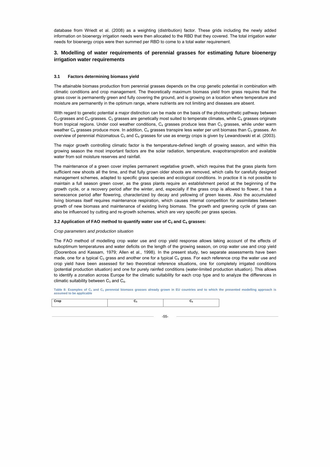
-55-

database from Wriedt et al. (2008) as a weighting (distribution) factor. These grids including the newly added information on bioenergy irrigation needs were then allocated to the RBD that they covered. The total irrigation water needs for bioenergy crops were then summed per RBD to come to a total water requirement.

3. Modelling of water requirements of perennial grasses for estimating future bioenergy irrigation water requirements

3.1 Factors determining biomass yield

The attainable biomass production from perennial grasses depends on the crop genetic potential in combination with climatic conditions and crop management. The theoretically maximum biomass yield from grass requires that the grass cover is permanently green and fully covering the ground, and is growing on a location where temperature and moisture are permanently in the optimum range, where nutrients are not limiting and diseases are absent.

With regard to genetic potential a major distinction can be made on the basis of the photosynthetic pathway between C3-grasses and C4-grasses. C3 grasses are genetically most suited to temperate climates, while C4 grasses originate from tropical regions. Under cool weather conditions, C4 grasses produce less than C3 grasses, while under warm weather C4 grasses produce more. In addition, C4 grasses transpire less water per unit biomass than C3 grasses. An overview of perennial rhizomatous C3 and C4 grasses for use as energy crops is given by Lewandowski et al. (2003).

The major growth controlling climatic factor is the temperature-defined length of growing season, and within this growing season the most important factors are the solar radiation, temperature, evapotranspiration and available water from soil moisture reserves and rainfall.

The maintenance of a green cover implies permanent vegetative growth, which requires that the grass plants form sufficient new shoots all the time, and that fully grown older shoots are removed, which calls for carefully designed management schemes, adapted to specific grass species and ecological conditions. In practice it is not possible to maintain a full season green cover, as the grass plants require an establishment period at the beginning of the growth cycle, or a recovery period after the winter, and, especially if the grass crop is allowed to flower, it has a senescence period after flowering, characterized by decay and yellowing of green leaves. Also the accumulated living biomass itself requires maintenance respiration, which causes internal competition for assimilates between growth of new biomass and maintenance of existing living biomass. The growth and greening cycle of grass can also be influenced by cutting and re-growth schemes, which are very specific per grass species.

3.2 Application of FAO method to quantify water use of C3 and C4 grasses:

Crop parameters and production situation

The FAO method of modelling crop water use and crop yield response allows taking account of the effects of suboptimum temperatures and water deficits on the length of the growing season, on crop water use and crop yield (Doorenbos and Kassam, 1979; Allen et al., 1998). In the present study, two separate assessments have been made, one for a typical C3 grass and another one for a typical C4 grass. For each reference crop the water use and crop yield have been assessed for two theoretical reference situations, one for completely irrigated conditions (potential production situation) and one for purely rainfed conditions (water-limited production situation). This allows to identify a zonation across Europe for the climatic suitability for each crop type and to analyze the differences in climatic suitability between C3 and C4.

Table 8: Examples of C3 and C4 perennial biomass grasses already grown in EU countries and to which the presented modelling approach is assumed to be applicable

Crop C3 C4

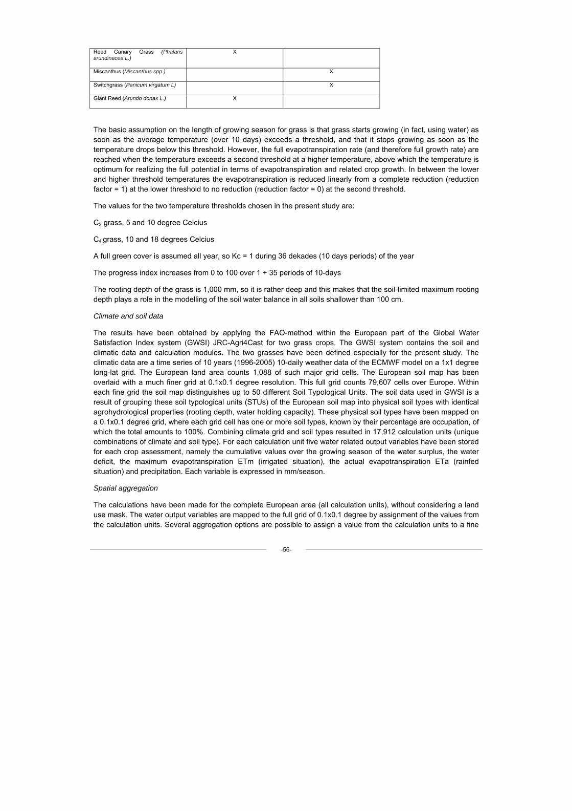
-56-

Reed Canary Grass (Phalaris arundinacea L.)

X

Miscanthus (Miscanthus spp.) X

Switchgrass (Panicum virgatum L) X

Giant Reed (Arundo donax L.) X

The basic assumption on the length of growing season for grass is that grass starts growing (in fact, using water) as soon as the average temperature (over 10 days) exceeds a threshold, and that it stops growing as soon as the temperature drops below this threshold. However, the full evapotranspiration rate (and therefore full growth rate) are reached when the temperature exceeds a second threshold at a higher temperature, above which the temperature is optimum for realizing the full potential in terms of evapotranspiration and related crop growth. In between the lower and higher threshold temperatures the evapotranspiration is reduced linearly from a complete reduction (reduction factor = 1) at the lower threshold to no reduction (reduction factor = 0) at the second threshold.

The values for the two temperature thresholds chosen in the present study are:

C3 grass, 5 and 10 degree Celcius

C4 grass, 10 and 18 degrees Celcius

A full green cover is assumed all year, so Kc = 1 during 36 dekades (10 days periods) of the year

The progress index increases from 0 to 100 over 1 + 35 periods of 10-days

The rooting depth of the grass is 1,000 mm, so it is rather deep and this makes that the soil-limited maximum rooting depth plays a role in the modelling of the soil water balance in all soils shallower than 100 cm.

Climate and soil data

The results have been obtained by applying the FAO-method within the European part of the Global Water Satisfaction Index system (GWSI) JRC-Agri4Cast for two grass crops. The GWSI system contains the soil and climatic data and calculation modules. The two grasses have been defined especially for the present study. The climatic data are a time series of 10 years (1996-2005) 10-daily weather data of the ECMWF model on a 1x1 degree long-lat grid. The European land area counts 1,088 of such major grid cells. The European soil map has been overlaid with a much finer grid at 0.1x0.1 degree resolution. This full grid counts 79,607 cells over Europe. Within each fine grid the soil map distinguishes up to 50 different Soil Typological Units. The soil data used in GWSI is a result of grouping these soil typological units (STUs) of the European soil map into physical soil types with identical agrohydrological properties (rooting depth, water holding capacity). These physical soil types have been mapped on a 0.1x0.1 degree grid, where each grid cell has one or more soil types, known by their percentage are occupation, of which the total amounts to 100%. Combining climate grid and soil types resulted in 17,912 calculation units (unique combinations of climate and soil type). For each calculation unit five water related output variables have been stored for each crop assessment, namely the cumulative values over the growing season of the water surplus, the water deficit, the maximum evapotranspiration ETm (irrigated situation), the actual evapotranspiration ETa (rainfed situation) and precipitation. Each variable is expressed in mm/season.

Spatial aggregation

The calculations have been made for the complete European area (all calculation units), without considering a land use mask. The water output variables are mapped to the full grid of 0.1x0.1 degree by assignment of the values from the calculation units. Several aggregation options are possible to assign a value from the calculation units to a fine

-57-

grid cell. In the present study we have chosen for the area weighted average value over each grid cell. Other reasonable alternatives are to take the value of the largest soil type within a cell, or the value of the best soil, or the value of the 25 percentile best soils in the cells. However, the area weighted value is the most unbiased value in a postprocessing, e.g, in order to combine these results with a land use mask and to distinguish regional yield patterns in relation with current agricultural areas.

The fine grid data are a basis for aggregation to NUTS-2 or national values, or to values at River Basin.

3.3 Translating water use into biomass potential yields

The maximum grass yield has been calculated by assuming characteristic water use efficiency values from the literature for C3 and C4 grasses. WUE is expressed in gram dry matter per kg used water. The range in WUE values is from 1 to 5 gr DM per kg ET. (Note that its inverse value is used as well. The corresponding range is expressed as between 1,000 and 200 kg ET per kg DM). As the basic conversion is 1 mm water = 10 m3 per hectare = 10,000 kg/ha, another expression of the range in WUE is from 10 to 50 kg DM per mm ET. We have chosen the WUE values as follows:

• WUE for C3 crops 30 kg DM per mm water use

• WUE for C4 crops 40 kg DM per mm water use

• nil (zero percent) harvest losses

With a range in ETa values of 200 to 1,300 mm over Europe , this leads to a range in theoretically maximum yield levels of 6,000 – 40,000 kg/hectare for C3 grasses, and 7000- 50,000 kg/hectare for C4 grasses. Note that on the same location the modelled ETa value for C3 and C4 are often different, due to differences in temperature response. These maximum yield levels are not attainable in reality for reasons explained earlier. A fraction of 70% of these maximum yields is a more realistic biomass yield ceiling, and 50% of these maximum yields is probably a fair target under intensive management.

When the choice is for extensive management and low external inputs, the value of the maximum yield maps is that it shows zones with relatively high and relatively low potential, and the differences in potential between typical C3 and C4 crops.

3.4 Results of the biomass assessment for C3 and C4 grasses

The assessment of the maximum yields leads to a set of four European yield maps showing a regional yield pattern for the following reference situations with a legend showing the range in yields

Table 9: Assessment of the maximum yields

Grass yield kg/ha C3 C4 Potential <5,000 to 40,000

(Map 12) <5,000 to >45,000 (Map 13)

Water limited <5000 to 20000 (Map 14)

<5,000 to 20,000 (Map 15)

Next, difference between C3 and C4 and potential and water limited yield levels can be analyzed, which results in four additional yield difference maps.

Table 10: Difference between C3 and C4 and potential and water limited yield levels

Grass yield kg/ha C3 grass C3-C4 difference C4 grass Potential grass yield <5,000 to 40,000 (Map 12) Up to + 8,000 in

northwest Europe <5,000 to >45,000 (Map 13)

-58-

Up to – 8,000 in south Europe (Map 16)

Pot – watlim difference

0-30,000 (Map 18)

0-35,000 (Map 19)

Water limited grass yield <5,000 to 20,000 (Map 14)

Up to + 8,000 in northwest Europe Up to – 4,000 in south and SE Europe (Map 17)

<5,000 to 20,000 (Map 15)

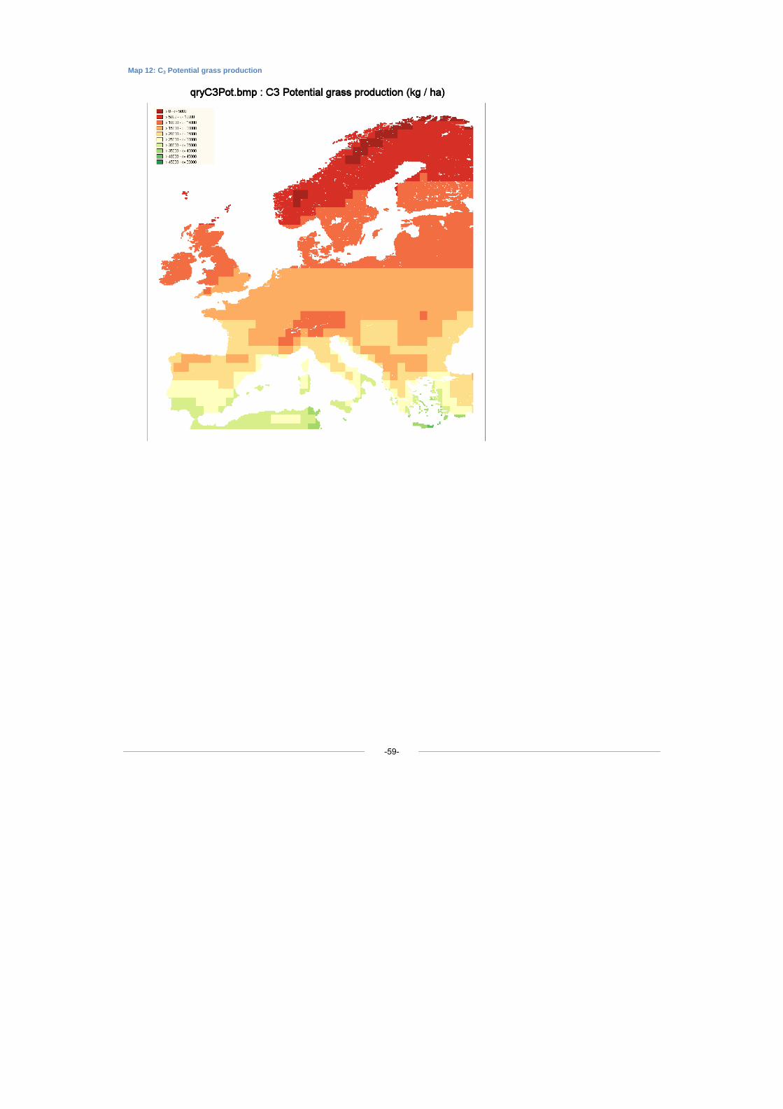
Map 12: C3 Potential grass production

-59-

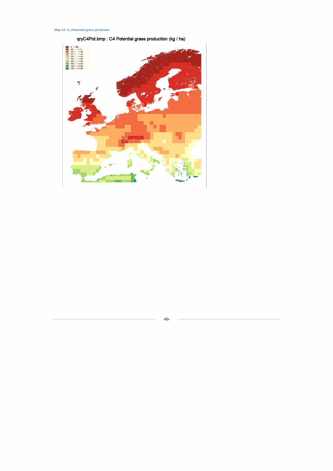
Map 13: C4 Potential grass prodction

-60-

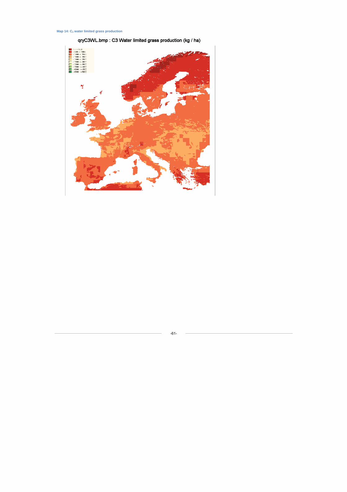
Map 14: C3 water limited grass production

-61-

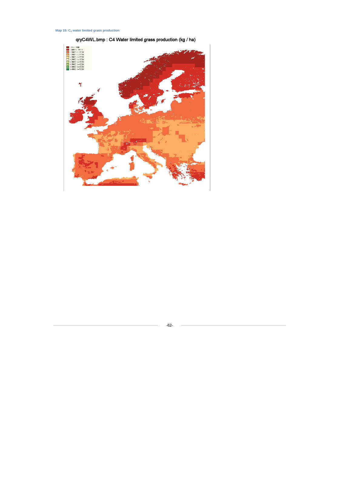
Map 15: C4 water limited grass production

-62-

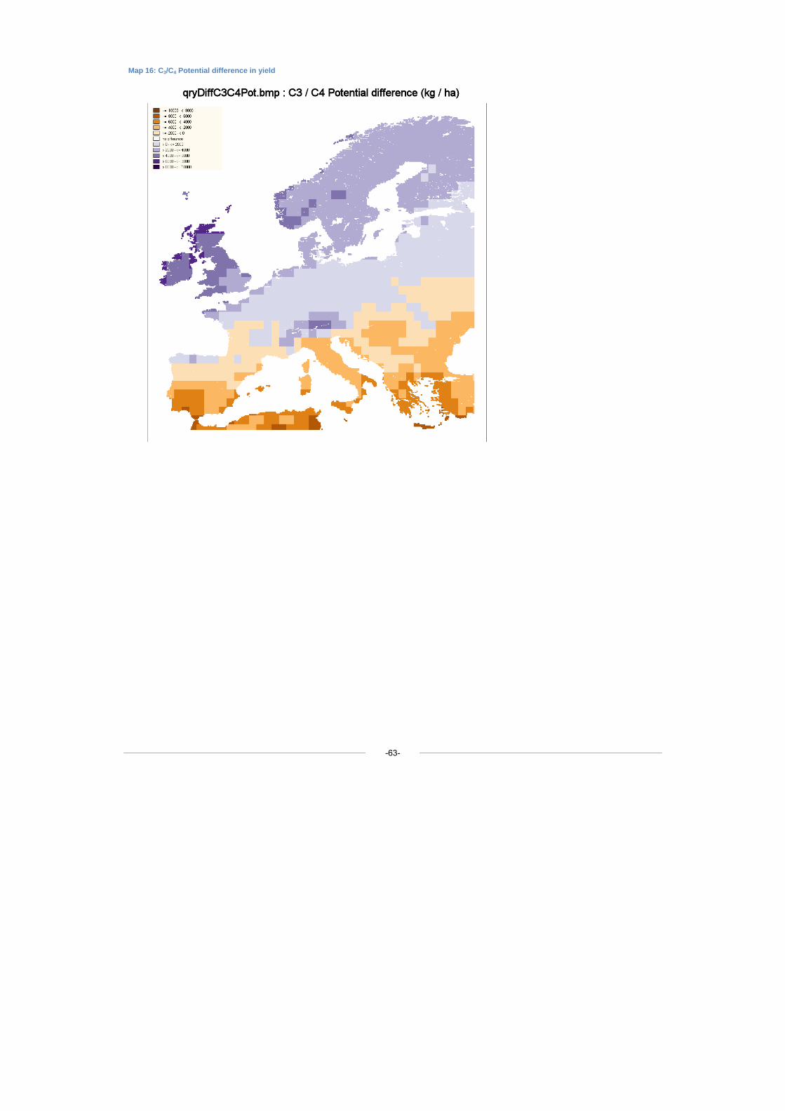
Map 16: C3/C4 Potential difference in yield

-63-

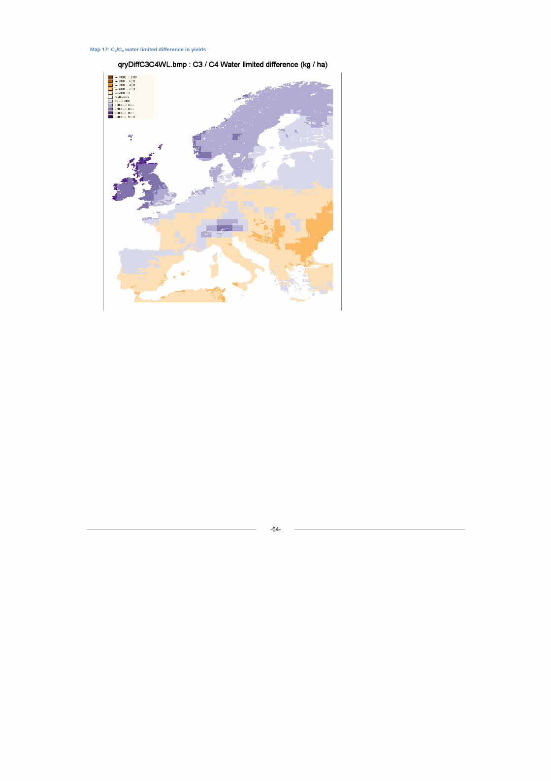
Map 17: C3/C4 water limited difference in yields

-64-

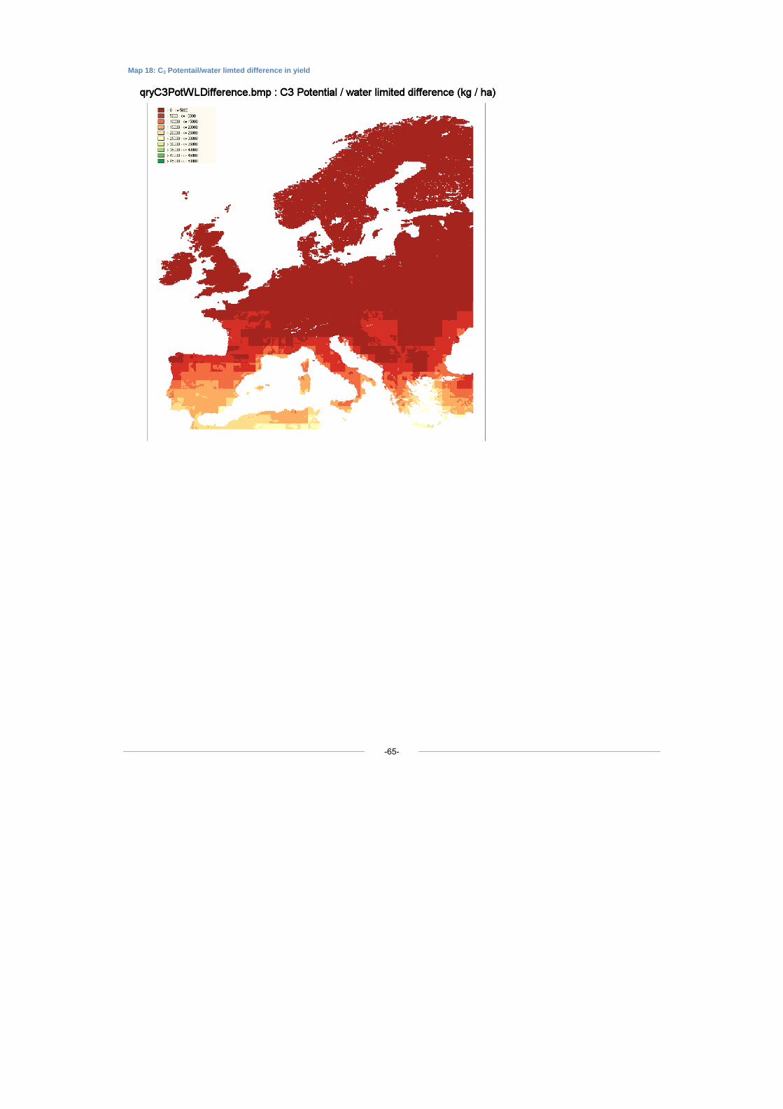
Map 18: C3 Potentail/water limted difference in yield

-65-

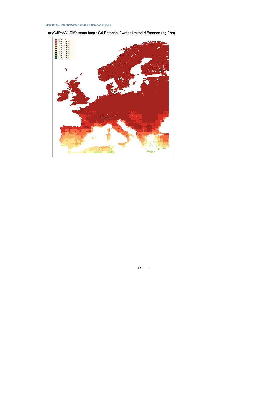
Map 19: C4 Potential/water limited difference in yield

-66-

-67-

It shows that the potential yield of C3 grass exceeds the C4 yields in the northern half of Europe and in the mountainous areas. The dividing line runs in the direction SWW-NEE. Just north of the dividing line are the Spanish Atlantic north coast, Brittany, Massif central and Alps in France, the Alpine and Carpathian regions, Poland and Bielorussia. The highest differences are in the areas with long cool summers, especially in Ireland and western UK, in the Alps and in a few areas in Norway. A second area with somewhat smaller differences in yield are Scandinavia and Finland, which have a short cool summer, and in the coastal strips along the Channel and in the North Sea region, which have slightly warmer summer than western UK. In the whole area of the northern European low plain from Brussels to Moscow the C3 grass has a slight advantage above the C4 grass. However, under water limited conditions the C4 grass has a relative advantage in those parts of the European plain where drought periods occur regularly in the summer, especially in soil regions with a lot of sandy soils, such as eastern Germany and Poland, except the coastal strip along the Baltic Sea. In northern European regions without water stress in the growing season the C3 grass maintains its advantage over C4 crops.

In the southern half of Europe potential grass yields of both C3 and C4 grasses increase southwards, but the C4 grass out-yields the C3 grass. The difference is largest under potential (irrigated) conditions in the far south

Also under water-limited conditions C4 grass out-yields the C3 grass. But the difference is levelled of by the increasing drought stress in the most southern regions.

The highest water-limited grass yields for C4 grasses are southern France, but not in the Mediterranean part, in northern Italy and all the area east of Warschau-Vienna, down to the west coast of the Black Sea, and West-Ukraine. The highest water-limited yields of C3 grass are slightly below the C4 yields and occur in the same regions as for C4 grass and for the Benelux countries. In all these areas a rather favourable balance exists between rainfall and evapotranspiration, during the entire growing season between winter and late autumn.

Conclusions for mapping of yield and water need levels:

From the above exercise we have derived a database specifying per 0.1x0.1 degree grid the total attainable and water limited yield for C3 and C4 crops and the related water need to arrive to this potential. From the latter we can also specify the irrigation water need per grid by subtracting the water need under total attainable yield with the under a water limited yield. The yields per location also provide the basis for the calculation of the potential energy yield from the C3 and C4 crops per location.

-68-

3.5 Translating biomass yield of perennial grasses over Europe into obtainable under current farming conditions fort the scenario assessments

The estimated theoretical maximum biomass productions for C3 and C4 perennial grasses assume optimum management conditions, which implies that a full green cover is reached soon after the start of the growing season, and sufficient nutrient availability from soil and fertilizer during the entire growing period. Two separate yield estimates have been made, one under full irrigation and one under purely rainfed conditions. These two production levels, potential and water-limited, should correspond with the highest yields observed in field experiments. In reality, the yields are often lower, due to suboptimum conditions such as nutrient shortage or incomplete plant cover.

For example, Consentino et al. (2007) report for a Miscanthus (a C4 grass) field experiment in Catania, Sicily, where the combined irrigation and nitrogen effects were studied, a maximum biomass yield of 27 T/ha dry matter under full nitrogen and water supply, 19 T/ha under full irrigation and low nitrogen level, and 17 T/ha under limited irrigation and nitrogen conditions. For the second year in the same multi-year experiment, the biomass yields were 18, 14.6 and 14.5 T/ha dry matter respectively. Note that there was not a purely rainfed situation in this trial. This shows inter-year yield variability, and important yield reductions due to limiting soil and water conditions. The annual biomass production for the same region (Sicily, NUTS itg1) according to to GWSI model was 35 tonnes DM ha-1 year-1 under potential conditions and 15 tonnes under water-limited conditions. In this case the maximum observed yield is 77% of the potential yield.

Lewandowski et al. (2003) provide a review of perennial grasses for use as energy crops in the US and Europe, and provide reported yield ranges from literature, per grass species and country. It is not clear under what kind of conditions these grasses were grown but we may assume that the highest yields are related to intensive crop management and our estimates of potential and water-limited biomass yields should correspond to these observed yields, while the lowest yields are probably below our water-limited yields, unless the reported yields are from irrigated fields.

The following table provides the comparison of yields reported by Lewandowski et al. (2003) and our yield estimates, per crop type and country.

Table 11: Comparison of observed and simulated biomass yield in some European countries for C3 and C4 grasses

Country C4 grass observed

C3 grass observed C4 simulated C3 simulated

Biomass yields are in tonnes DM ha-1 year-1

sw switch gra

mi Miscanthus

gr giant reed rcg reed canary pot potential wl water-lim Pot potential wl water- lim

Finland 5-12 (rcg) 8-11 (pot)

8-10 (wl)

Sweden 5-12 (rcg) 7-12 (pot)

7-12 (wl)

Denmark 5-15 (mi) 10-11 (pot)

10-10 (wl)

Britain 11 (sw) 6-12 (rcg) 5-13 (pot) 10-16 (pot)

10-15 (mi) 5-13 (wl) 10-14 (wl)

Germany 4-30 (mi) 15-20 (gr) 12-16 (pot) 14-16 (pot)

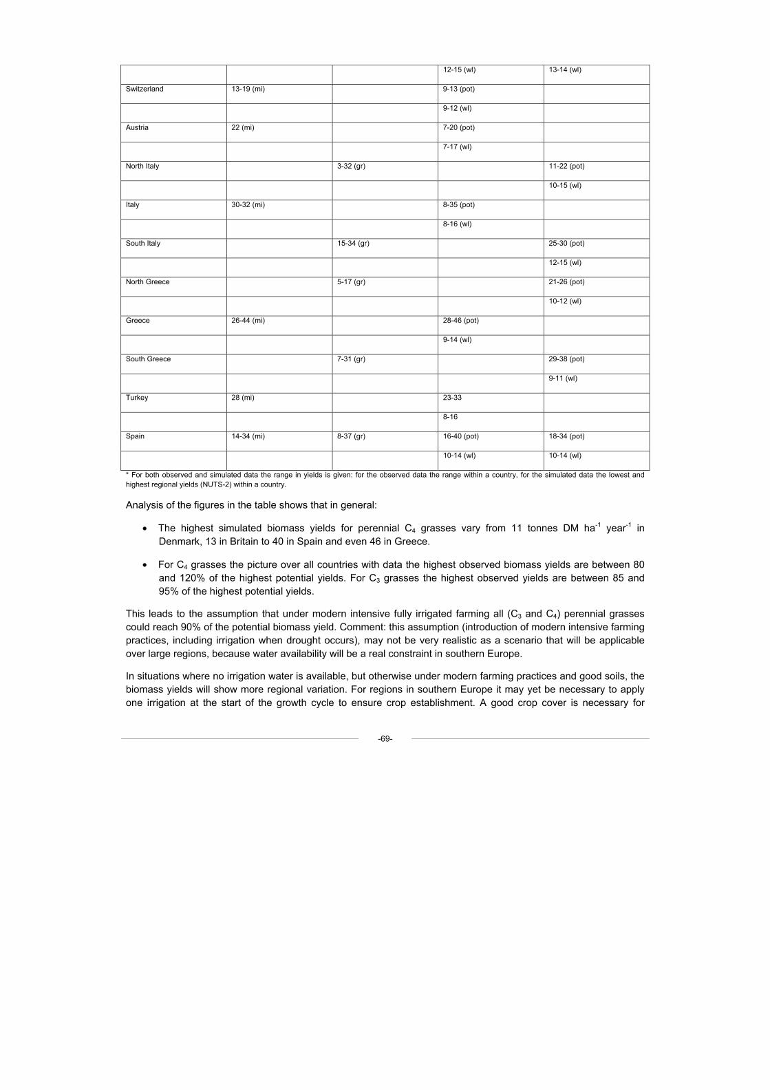
-69-

12-15 (wl) 13-14 (wl)

Switzerland 13-19 (mi) 9-13 (pot)

9-12 (wl)

Austria 22 (mi) 7-20 (pot)

7-17 (wl)

North Italy 3-32 (gr) 11-22 (pot)

10-15 (wl)

Italy 30-32 (mi) 8-35 (pot)

8-16 (wl)

South Italy 15-34 (gr) 25-30 (pot)

12-15 (wl)

North Greece 5-17 (gr) 21-26 (pot)

10-12 (wl)

Greece 26-44 (mi) 28-46 (pot)

9-14 (wl)

South Greece 7-31 (gr) 29-38 (pot)

9-11 (wl)

Turkey 28 (mi) 23-33

8-16

Spain 14-34 (mi) 8-37 (gr) 16-40 (pot) 18-34 (pot)

10-14 (wl) 10-14 (wl)

* For both observed and simulated data the range in yields is given: for the observed data the range within a country, for the simulated data the lowest and highest regional yields (NUTS-2) within a country.

Analysis of the figures in the table shows that in general:

• The highest simulated biomass yields for perennial C4 grasses vary from 11 tonnes DM ha-1 year-1 in Denmark, 13 in Britain to 40 in Spain and even 46 in Greece.

• For C4 grasses the picture over all countries with data the highest observed biomass yields are between 80 and 120% of the highest potential yields. For C3 grasses the highest observed yields are between 85 and 95% of the highest potential yields.

This leads to the assumption that under modern intensive fully irrigated farming all (C3 and C4) perennial grasses could reach 90% of the potential biomass yield. Comment: this assumption (introduction of modern intensive farming practices, including irrigation when drought occurs), may not be very realistic as a scenario that will be applicable over large regions, because water availability will be a real constraint in southern Europe.

In situations where no irrigation water is available, but otherwise under modern farming practices and good soils, the biomass yields will show more regional variation. For regions in southern Europe it may yet be necessary to apply one irrigation at the start of the growth cycle to ensure crop establishment. A good crop cover is necessary for

-70-

reaching the full water-limited yield. The assumption of modern farm technology is justified, as large scale biomass cropping will be organized as a new agricultural business which will not evolve from traditional farming.

The basic set of assumptions for the yield level is that the production ceiling is set at 90% of the potential production, but will not exceed the water-limited production. This can be assessed easily by taking the lowest value of the following two yield levels: (90% of potential yield) and (100% of the water-limited yield).

Comment 1: This assumption means that in areas with sufficient rainfall (northern half of Europe) the attainable production will be close to 90% of the potential yield, but especially in southern Europe the rainfed biomass production will be down to 50 or 25% of the maximum irrigated production.

Comment 2: It appears from the observed yield data however, that for the southern European countries the lowest observed yields are above the water-limited yields, implying that the bio-energy grasses are irrigated at least partly. Yet the assumption that the large scale introduction of new biomass crops should rely largely on rainfed cropping seems justified.

In situation of extensive arable farming and low soil quality (shallow, or otherwise marginally productive soils) the biomass production will be lower than under intensive farming. We assume that the range of yield levels for these situations can be found in the tail of the observed yields, e.g. below the midyield in the range of observed yields per region (or per country). In reality the variability in biomass yields under extensive farming systems will be high. A reasonable first guess would be to assess the obtainable biomass yield under extensive arable farming as the lowest yield of the following two: (50% of the potential yield) and (80% of the water limited yield).

-71-

Summary on assessment of attainable grass yield

In summary we can derive from the set of regional mean potential and water-limited yields for C3 and C4 perennial grasses three attainable biomass yield levels, according to the type of cropping:

• Modern fully irrigated cropping: all grasses could reach 90% of the potential biomass yield.

• Modern rainfed cropping (apart from crop establishment irrigation): attainable grass yield equals the lowest value of the following two yield levels: (90% of potential yield) and (100% of the water-limited yield).

• Extensive cropping: the lowest yield of the following two: (50% of the potential yield) and (80% of the water limited yield).

These 3 yield levels have been used in the scenario studies to estimate the final total yield levels of C3 and C4 biomass grasses.

In Table 12 an overview is given of these three yield levels in different EU regions as modeled with the Global Water Satisfaction Index system (GWSI) described above and converted into attainable yields according to the rules described above in this Section.

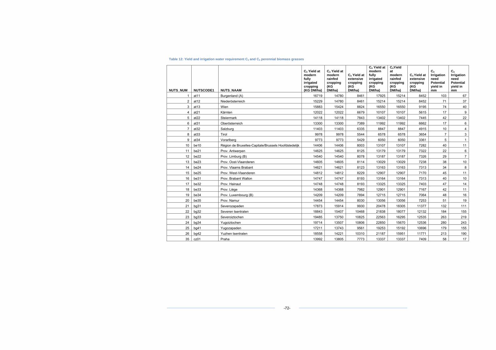
Table 12: Yield and irrigation water requirement C3 and C4 perennial biomass grasses

NUTS_NUM NUTSCODE1 NUTS_NAAM

C3 Yield at modern fully irrigated cropping (KG DM/ha)

C3 Yield at modern rainfed cropping (KG DM/ha)

C3 Yield at extensive cropping (KG DM/ha)

C4 Yield at modern fully irrigated cropping (KG DM/ha)

C4Yield at modern rainfed cropping (KG DM/ha)

C4 Yield at extensive cropping (KG DM/ha)

C3 Irrigation need Potential yield in mm

C4 Irrigation need Potential yield in mm

1 at11 Burgenland (A) 16719 14780 8461 17925 15214 8452 103 67 2 at12 Niederösterreich 15229 14780 8461 15214 15214 8452 71 37 3 at13 Wien 15883 15424 8824 16550 16550 9195 74 40 4 at21 Kärnten 12022 12022 6679 10107 10107 5615 17 9 5 at22 Steiermark 14118 14118 7843 13402 13402 7445 42 22 6 at31 Oberösterreich 13300 13300 7389 11992 11992 6662 17 6 7 at32 Salzburg 11403 11403 6335 8847 8847 4915 10 4 8 at33 Tirol 9978 9978 5544 6578 6578 3654 7 3 9 at34 Vorarlberg 9773 9773 5429 6050 6050 3361 5 1

10 be10 Région de Bruxelles-Capitale/Brussels Hoofdstedelijk 14406 14406 8003 13107 13107 7282 40 11 11 be21 Prov. Antwerpen 14625 14625 8125 13179 13179 7322 22 6 12 be22 Prov. Limburg (B) 14540 14540 8078 13187 13187 7326 29 7 13 be23 Prov. Oost-Vlaanderen 14605 14605 8114 13029 13029 7238 38 10 14 be24 Prov. Vlaams Brabant 14621 14621 8123 13163 13163 7313 34 8 15 be25 Prov. West-Vlaanderen 14812 14812 8229 12907 12907 7170 45 11 16 be31 Prov. Brabant Wallon 14747 14747 8193 13164 13164 7313 40 10 17 be32 Prov. Hainaut 14748 14748 8193 13325 13325 7403 47 14 18 be33 Prov. Liège 14368 14368 7982 12901 12901 7167 42 11 19 be34 Prov. Luxembourg (B) 14209 14209 7894 12715 12715 7064 48 16 20 be35 Prov. Namur 14454 14454 8030 13056 13056 7253 51 19 21 bg31 Severozapaden 17873 15914 9930 20478 18305 11377 132 111 22 bg32 Severen tsentralen 18843 15407 10468 21838 18077 12132 184 155 23 bg33 Severoiztochen 19485 13750 10825 22563 16295 12535 263 219 24 bg34 Yugoiztochen 19714 13507 10806 22850 15670 12536 280 243 25 bg41 Yugozapaden 17211 13743 9561 19253 15192 10696 179 155 26 bg42 Yuzhen tsentralen 18558 14221 10310 21187 15951 11771 213 190 35 cz01 Praha 13992 13805 7773 13337 13337 7409 58 17

-72-

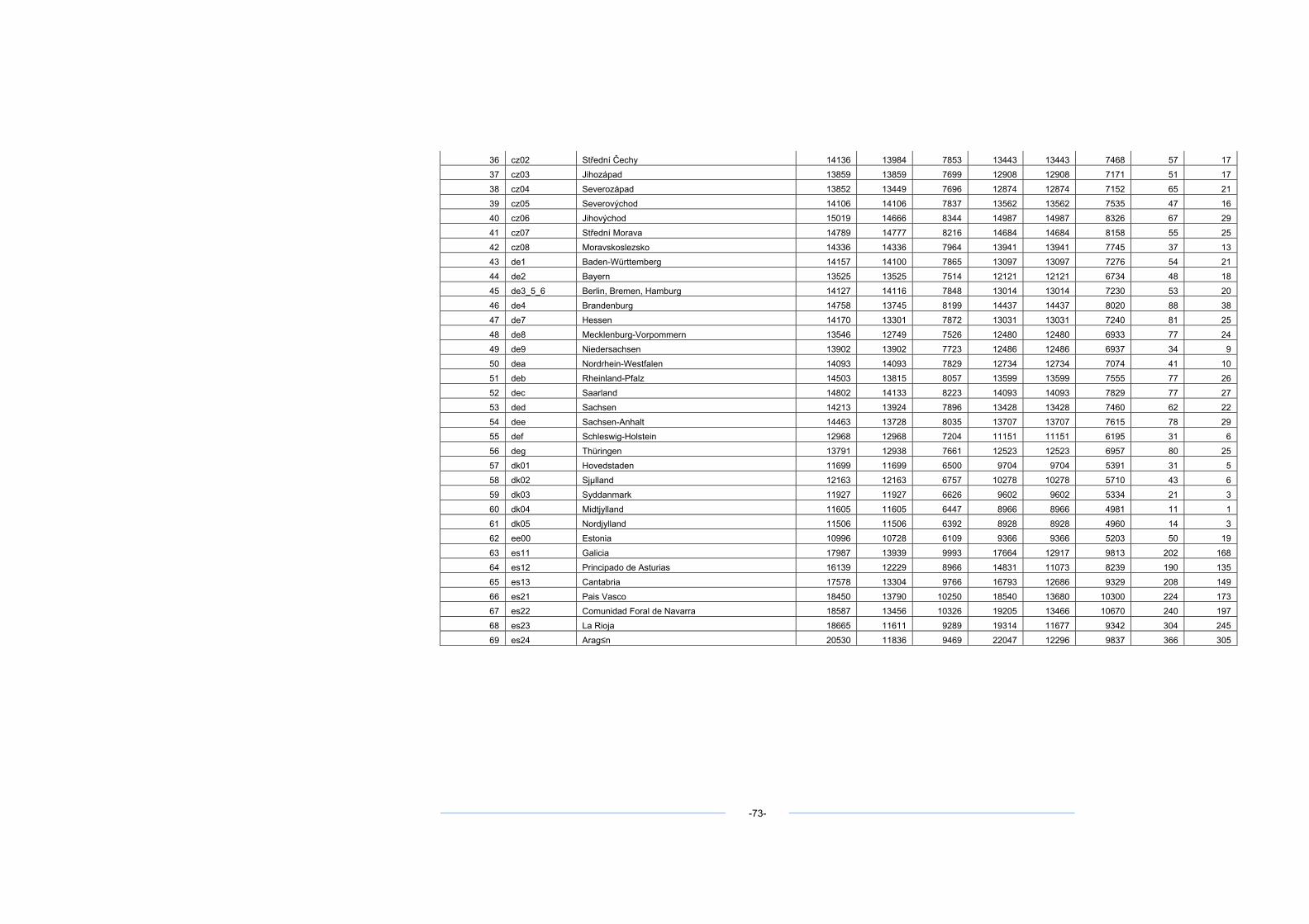
36 cz02 Střední Čechy 14136 13984 7853 13443 13443 7468 57 17 37 cz03 Jihozápad 13859 13859 7699 12908 12908 7171 51 17 38 cz04 Severozápad 13852 13449 7696 12874 12874 7152 65 21 39 cz05 Severovýchod 14106 14106 7837 13562 13562 7535 47 16 40 cz06 Jihovýchod 15019 14666 8344 14987 14987 8326 67 29 41 cz07 Střední Morava 14789 14777 8216 14684 14684 8158 55 25 42 cz08 Moravskoslezsko 14336 14336 7964 13941 13941 7745 37 13 43 de1 Baden-Württemberg 14157 14100 7865 13097 13097 7276 54 21 44 de2 Bayern 13525 13525 7514 12121 12121 6734 48 18 45 de3_5_6 Berlin, Bremen, Hamburg 14127 14116 7848 13014 13014 7230 53 20 46 de4 Brandenburg 14758 13745 8199 14437 14437 8020 88 38 47 de7 Hessen 14170 13301 7872 13031 13031 7240 81 25 48 de8 Mecklenburg-Vorpommern 13546 12749 7526 12480 12480 6933 77 24 49 de9 Niedersachsen 13902 13902 7723 12486 12486 6937 34 9 50 dea Nordrhein-Westfalen 14093 14093 7829 12734 12734 7074 41 10 51 deb Rheinland-Pfalz 14503 13815 8057 13599 13599 7555 77 26 52 dec Saarland 14802 14133 8223 14093 14093 7829 77 27 53 ded Sachsen 14213 13924 7896 13428 13428 7460 62 22 54 dee Sachsen-Anhalt 14463 13728 8035 13707 13707 7615 78 29 55 def Schleswig-Holstein 12968 12968 7204 11151 11151 6195 31 6 56 deg Thüringen 13791 12938 7661 12523 12523 6957 80 25 57 dk01 Hovedstaden 11699 11699 6500 9704 9704 5391 31 5 58 dk02 Sjµlland 12163 12163 6757 10278 10278 5710 43 6 59 dk03 Syddanmark 11927 11927 6626 9602 9602 5334 21 3 60 dk04 Midtjylland 11605 11605 6447 8966 8966 4981 11 1 61 dk05 Nordjylland 11506 11506 6392 8928 8928 4960 14 3 62 ee00 Estonia 10996 10728 6109 9366 9366 5203 50 19 63 es11 Galicia 17987 13939 9993 17664 12917 9813 202 168 64 es12 Principado de Asturias 16139 12229 8966 14831 11073 8239 190 135 65 es13 Cantabria 17578 13304 9766 16793 12686 9329 208 149 66 es21 Pais Vasco 18450 13790 10250 18540 13680 10300 224 173 67 es22 Comunidad Foral de Navarra 18587 13456 10326 19205 13466 10670 240 197 68 es23 La Rioja 18665 11611 9289 19314 11677 9342 304 245 69 es24 Arag≤n 20530 11836 9469 22047 12296 9837 366 305

-73-

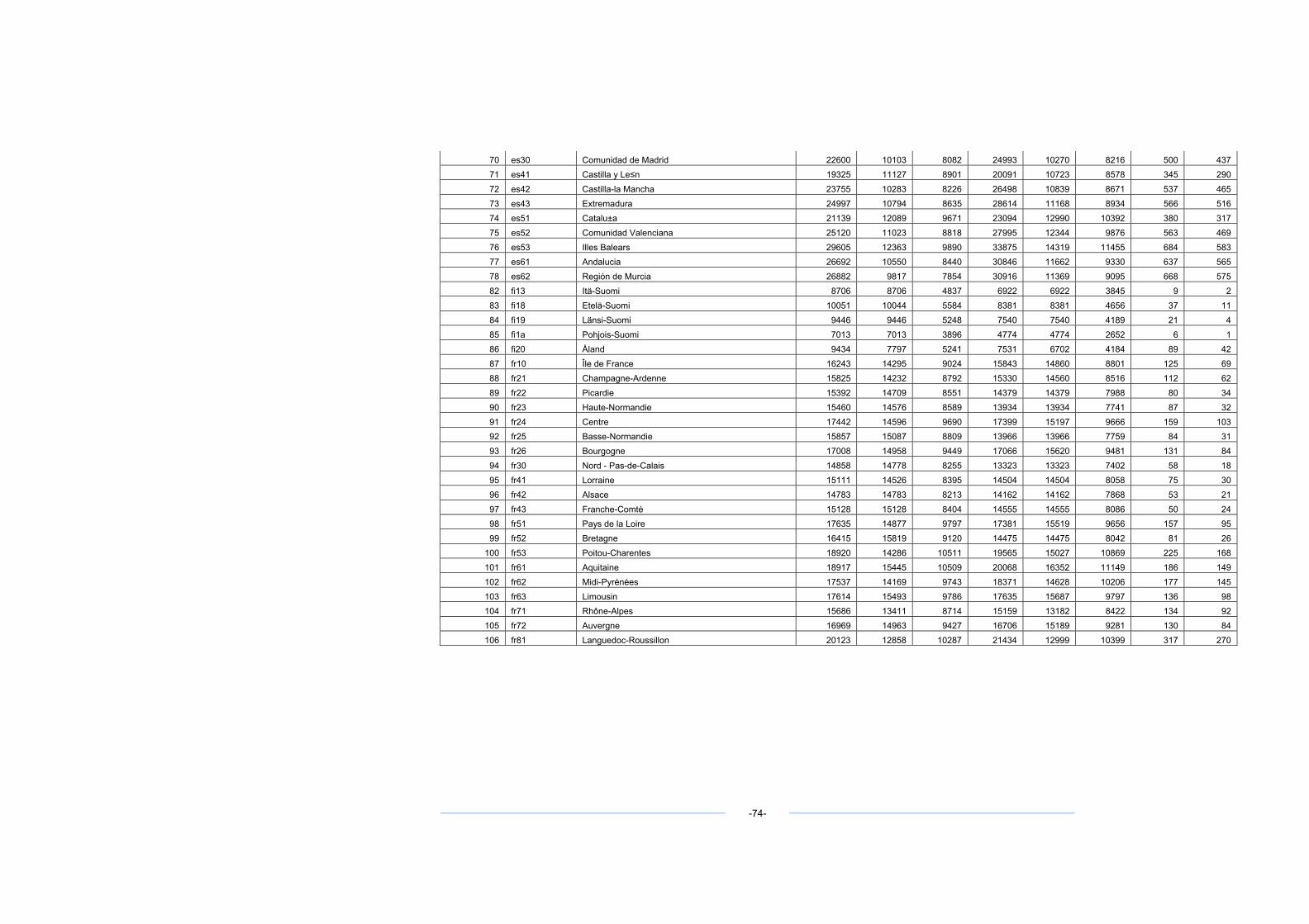
70 es30 Comunidad de Madrid 22600 10103 8082 24993 10270 8216 500 437 71 es41 Castilla y Le≤n 19325 11127 8901 20091 10723 8578 345 290 72 es42 Castilla-la Mancha 23755 10283 8226 26498 10839 8671 537 465 73 es43 Extremadura 24997 10794 8635 28614 11168 8934 566 516 74 es51 Catalu±a 21139 12089 9671 23094 12990 10392 380 317 75 es52 Comunidad Valenciana 25120 11023 8818 27995 12344 9876 563 469 76 es53 Illes Balears 29605 12363 9890 33875 14319 11455 684 583 77 es61 Andalucia 26692 10550 8440 30846 11662 9330 637 565 78 es62 Región de Murcia 26882 9817 7854 30916 11369 9095 668 575 82 fi13 Itä-Suomi 8706 8706 4837 6922 6922 3845 9 2 83 fi18 Etelä-Suomi 10051 10044 5584 8381 8381 4656 37 11 84 fi19 Länsi-Suomi 9446 9446 5248 7540 7540 4189 21 4 85 fi1a Pohjois-Suomi 7013 7013 3896 4774 4774 2652 6 1 86 fi20 Åland 9434 7797 5241 7531 6702 4184 89 42 87 fr10 Île de France 16243 14295 9024 15843 14860 8801 125 69 88 fr21 Champagne-Ardenne 15825 14232 8792 15330 14560 8516 112 62 89 fr22 Picardie 15392 14709 8551 14379 14379 7988 80 34 90 fr23 Haute-Normandie 15460 14576 8589 13934 13934 7741 87 32 91 fr24 Centre 17442 14596 9690 17399 15197 9666 159 103 92 fr25 Basse-Normandie 15857 15087 8809 13966 13966 7759 84 31 93 fr26 Bourgogne 17008 14958 9449 17066 15620 9481 131 84 94 fr30 Nord - Pas-de-Calais 14858 14778 8255 13323 13323 7402 58 18 95 fr41 Lorraine 15111 14526 8395 14504 14504 8058 75 30 96 fr42 Alsace 14783 14783 8213 14162 14162 7868 53 21 97 fr43 Franche-Comté 15128 15128 8404 14555 14555 8086 50 24 98 fr51 Pays de la Loire 17635 14877 9797 17381 15519 9656 157 95 99 fr52 Bretagne 16415 15819 9120 14475 14475 8042 81 26

100 fr53 Poitou-Charentes 18920 14286 10511 19565 15027 10869 225 168 101 fr61 Aquitaine 18917 15445 10509 20068 16352 11149 186 149 102 fr62 Midi-Pyrénées 17537 14169 9743 18371 14628 10206 177 145 103 fr63 Limousin 17614 15493 9786 17635 15687 9797 136 98 104 fr71 Rhône-Alpes 15686 13411 8714 15159 13182 8422 134 92 105 fr72 Auvergne 16969 14963 9427 16706 15189 9281 130 84 106 fr81 Languedoc-Roussillon 20123 12858 10287 21434 12999 10399 317 270

-74-

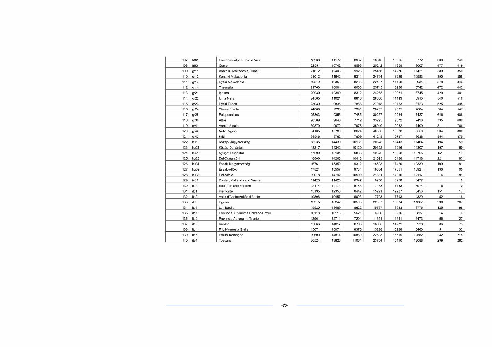
107 fr82 Provence-Alpes-Côte d'Azur 18238 11172 8937 18846 10965 8772 303 249 108 fr83 Corse 22551 10742 8593 25212 11259 9007 477 419 109 gr11 Anatoliki Makedonia, Thraki 21672 12403 9923 25456 14276 11421 389 350 110 gr12 Kentriki Makedonia 21012 11642 9314 24794 13229 10583 390 358 111 gr13 Dytiki Makedonia 19519 10356 8285 22497 11168 8934 378 346 112 gr14 Thessalia 21760 10004 8003 25745 10928 8742 472 442 113 gr21 Ipeiros 20930 10390 8312 24268 10931 8745 429 401 114 gr22 Ionia Nisia 24505 11021 8816 28600 11143 8915 540 516 115 gr23 Dytiki Ellada 23030 9835 7868 27048 10153 8123 525 498 116 gr24 Sterea Ellada 24089 9238 7391 28259 9505 7604 584 547 117 gr25 Peloponnisos 25863 9356 7485 30257 9284 7427 646 608 118 gr30 Attiki 28509 9640 7712 33225 9372 7498 735 689 119 gr41 Voreio Aigaio 30879 9972 7978 35910 9262 7409 811 766 120 gr42 Notio Aigaio 34105 10780 8624 40596 10688 8550 904 860 121 gr43 Kriti 34546 9762 7809 41218 10797 8638 954 875 122 hu10 Közép-Magyarország 18235 14430 10131 20528 16443 11404 194 159 123 hu21 Közép-Dunántúl 18217 14342 10120 20352 16216 11307 197 160 124 hu22 Nyugat-Dunántúl 17699 15134 9833 19376 16968 10765 151 114 125 hu23 Dél-Dunántúl·l 18806 14268 10448 21093 16128 11718 221 183 126 hu31 Észak-Magyarország 16761 15350 9312 18593 17420 10330 109 81 127 hu32 Észak-Alföld 17521 15557 9734 19664 17651 10924 130 105 128 hu33 Dél-Alföld 19078 14792 10599 21811 17010 12117 214 181 129 ie01 Border, Midlands and Western 11425 11425 6347 6258 6258 3477 1 0 130 ie02 Southern and Eastern 12174 12174 6763 7153 7153 3974 6 0 131 itc1 Piemonte 15195 12350 8442 15221 12227 8456 151 117 132 itc2 Valle d'Aosta/Vallée d'Aoste 10806 10457 6003 7793 7793 4329 52 18 133 itc3 Liguria 19915 13242 10593 22067 13834 11067 296 267 134 itc4 Lombardia 15520 13489 8622 15797 13623 8776 125 98 135 itd1 Provincia Autonoma Bolzano-Bozen 10118 10118 5621 6906 6906 3837 14 6 136 itd2 Provincia Autonoma Trento 12961 12711 7201 11651 11651 6473 56 27 137 itd3 Veneto 15666 14817 8703 16088 14972 8938 86 73 138 itd4 Friuli-Venezia Giulia 15074 15074 8375 15228 15228 8460 51 32 139 itd5 Emilia-Romagna 19600 14814 10889 22593 16519 12552 232 215 140 ite1 Toscana 20524 13826 11061 23754 15110 12088 299 282

-75-

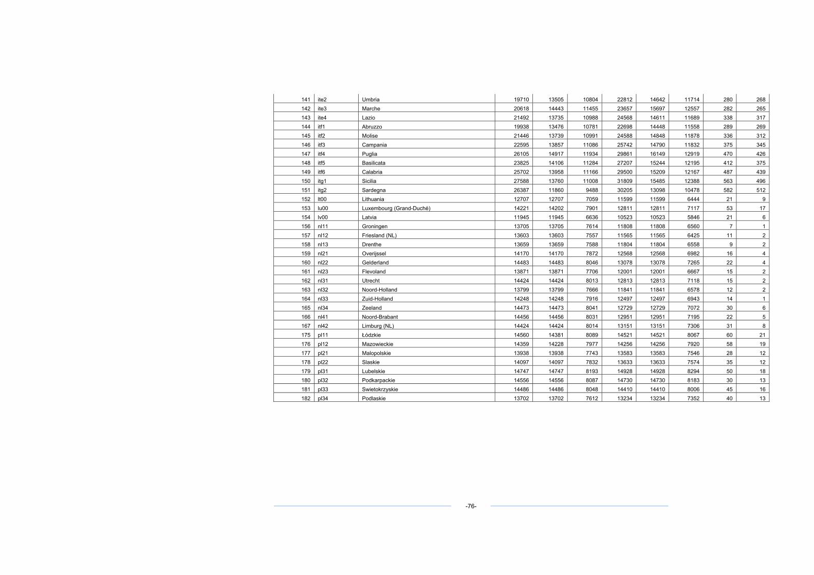
141 ite2 Umbria 19710 13505 10804 22812 14642 11714 280 268 142 ite3 Marche 20618 14443 11455 23657 15697 12557 282 265 143 ite4 Lazio 21492 13735 10988 24568 14611 11689 338 317 144 itf1 Abruzzo 19938 13476 10781 22698 14448 11558 289 269 145 itf2 Molise 21446 13739 10991 24588 14848 11878 336 312 146 itf3 Campania 22595 13857 11086 25742 14790 11832 375 345 147 itf4 Puglia 26105 14917 11934 29861 16149 12919 470 426 148 itf5 Basilicata 23825 14106 11284 27207 15244 12195 412 375 149 itf6 Calabria 25702 13958 11166 29500 15209 12167 487 439 150 itg1 Sicilia 27588 13760 11008 31809 15485 12388 563 496 151 itg2 Sardegna 26387 11860 9488 30205 13098 10478 582 512 152 lt00 Lithuania 12707 12707 7059 11599 11599 6444 21 9 153 lu00 Luxembourg (Grand-Duché) 14221 14202 7901 12811 12811 7117 53 17 154 lv00 Latvia 11945 11945 6636 10523 10523 5846 21 6 156 nl11 Groningen 13705 13705 7614 11808 11808 6560 7 1 157 nl12 Friesland (NL) 13603 13603 7557 11565 11565 6425 11 2 158 nl13 Drenthe 13659 13659 7588 11804 11804 6558 9 2 159 nl21 Overijssel 14170 14170 7872 12568 12568 6982 16 4 160 nl22 Gelderland 14483 14483 8046 13078 13078 7265 22 4 161 nl23 Flevoland 13871 13871 7706 12001 12001 6667 15 2 162 nl31 Utrecht 14424 14424 8013 12813 12813 7118 15 2 163 nl32 Noord-Holland 13799 13799 7666 11841 11841 6578 12 2 164 nl33 Zuid-Holland 14248 14248 7916 12497 12497 6943 14 1 165 nl34 Zeeland 14473 14473 8041 12729 12729 7072 30 6 166 nl41 Noord-Brabant 14456 14456 8031 12951 12951 7195 22 5 167 nl42 Limburg (NL) 14424 14424 8014 13151 13151 7306 31 8 175 pl11 Łódzkie 14560 14381 8089 14521 14521 8067 60 21 176 pl12 Mazowieckie 14359 14228 7977 14256 14256 7920 58 19 177 pl21 Malopolskie 13938 13938 7743 13583 13583 7546 28 12 178 pl22 Slaskie 14097 14097 7832 13633 13633 7574 35 12 179 pl31 Lubelskie 14747 14747 8193 14928 14928 8294 50 18 180 pl32 Podkarpackie 14556 14556 8087 14730 14730 8183 30 13 181 pl33 Swietokrzyskie 14486 14486 8048 14410 14410 8006 45 16 182 pl34 Podlaskie 13702 13702 7612 13234 13234 7352 40 13

-76-

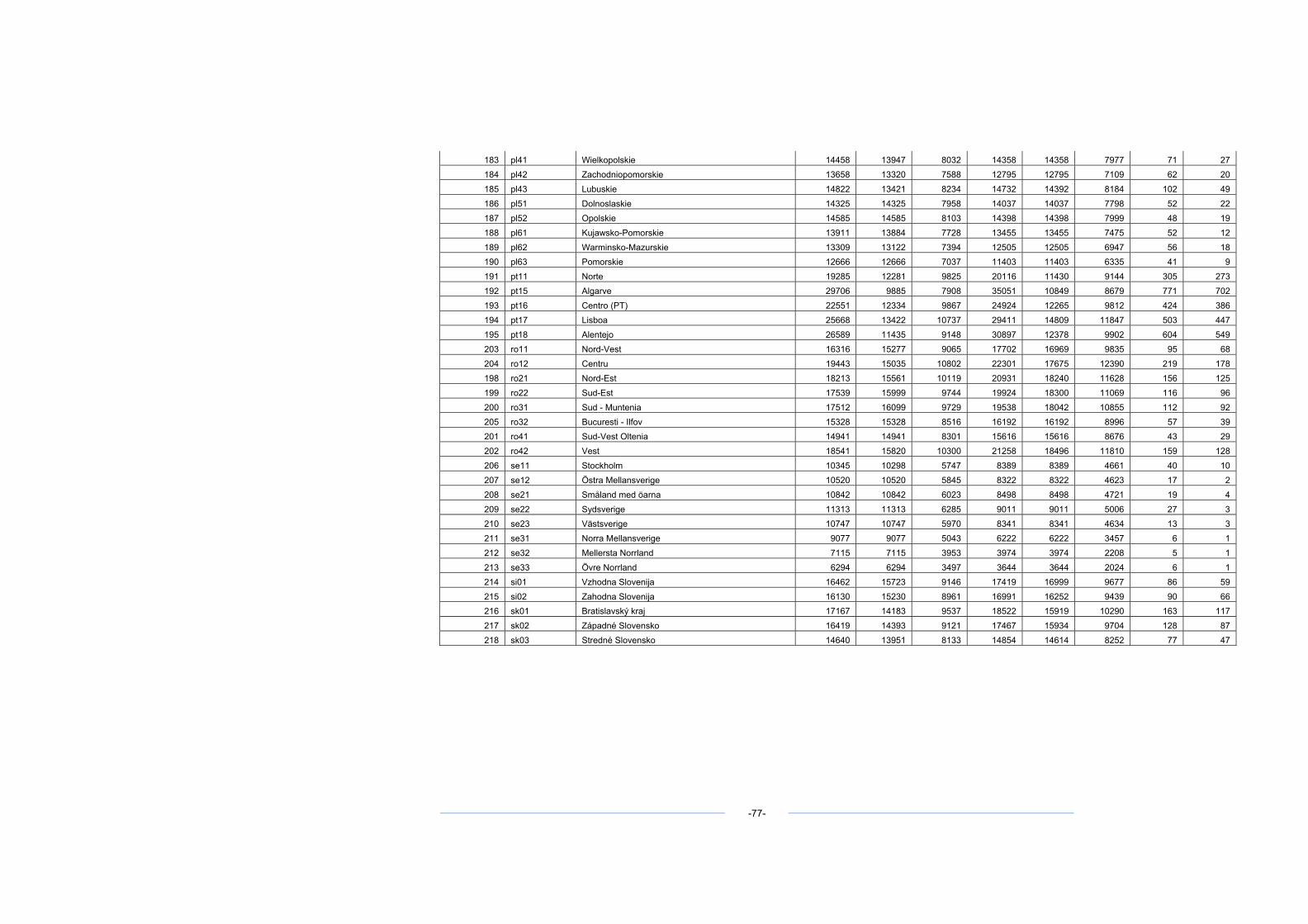
183 pl41 Wielkopolskie 14458 13947 8032 14358 14358 7977 71 27 184 pl42 Zachodniopomorskie 13658 13320 7588 12795 12795 7109 62 20 185 pl43 Lubuskie 14822 13421 8234 14732 14392 8184 102 49 186 pl51 Dolnoslaskie 14325 14325 7958 14037 14037 7798 52 22 187 pl52 Opolskie 14585 14585 8103 14398 14398 7999 48 19 188 pl61 Kujawsko-Pomorskie 13911 13884 7728 13455 13455 7475 52 12 189 pl62 Warminsko-Mazurskie 13309 13122 7394 12505 12505 6947 56 18 190 pl63 Pomorskie 12666 12666 7037 11403 11403 6335 41 9 191 pt11 Norte 19285 12281 9825 20116 11430 9144 305 273 192 pt15 Algarve 29706 9885 7908 35051 10849 8679 771 702 193 pt16 Centro (PT) 22551 12334 9867 24924 12265 9812 424 386 194 pt17 Lisboa 25668 13422 10737 29411 14809 11847 503 447 195 pt18 Alentejo 26589 11435 9148 30897 12378 9902 604 549 203 ro11 Nord-Vest 16316 15277 9065 17702 16969 9835 95 68 204 ro12 Centru 19443 15035 10802 22301 17675 12390 219 178 198 ro21 Nord-Est 18213 15561 10119 20931 18240 11628 156 125 199 ro22 Sud-Est 17539 15999 9744 19924 18300 11069 116 96 200 ro31 Sud - Muntenia 17512 16099 9729 19538 18042 10855 112 92 205 ro32 Bucuresti - Ilfov 15328 15328 8516 16192 16192 8996 57 39 201 ro41 Sud-Vest Oltenia 14941 14941 8301 15616 15616 8676 43 29 202 ro42 Vest 18541 15820 10300 21258 18496 11810 159 128 206 se11 Stockholm 10345 10298 5747 8389 8389 4661 40 10 207 se12 Östra Mellansverige 10520 10520 5845 8322 8322 4623 17 2 208 se21 Småland med öarna 10842 10842 6023 8498 8498 4721 19 4 209 se22 Sydsverige 11313 11313 6285 9011 9011 5006 27 3 210 se23 Västsverige 10747 10747 5970 8341 8341 4634 13 3 211 se31 Norra Mellansverige 9077 9077 5043 6222 6222 3457 6 1 212 se32 Mellersta Norrland 7115 7115 3953 3974 3974 2208 5 1 213 se33 Övre Norrland 6294 6294 3497 3644 3644 2024 6 1 214 si01 Vzhodna Slovenija 16462 15723 9146 17419 16999 9677 86 59 215 si02 Zahodna Slovenija 16130 15230 8961 16991 16252 9439 90 66 216 sk01 Bratislavský kraj 17167 14183 9537 18522 15919 10290 163 117 217 sk02 Západné Slovensko 16419 14393 9121 17467 15934 9704 128 87 218 sk03 Stredné Slovensko 14640 13951 8133 14854 14614 8252 77 47

-77-

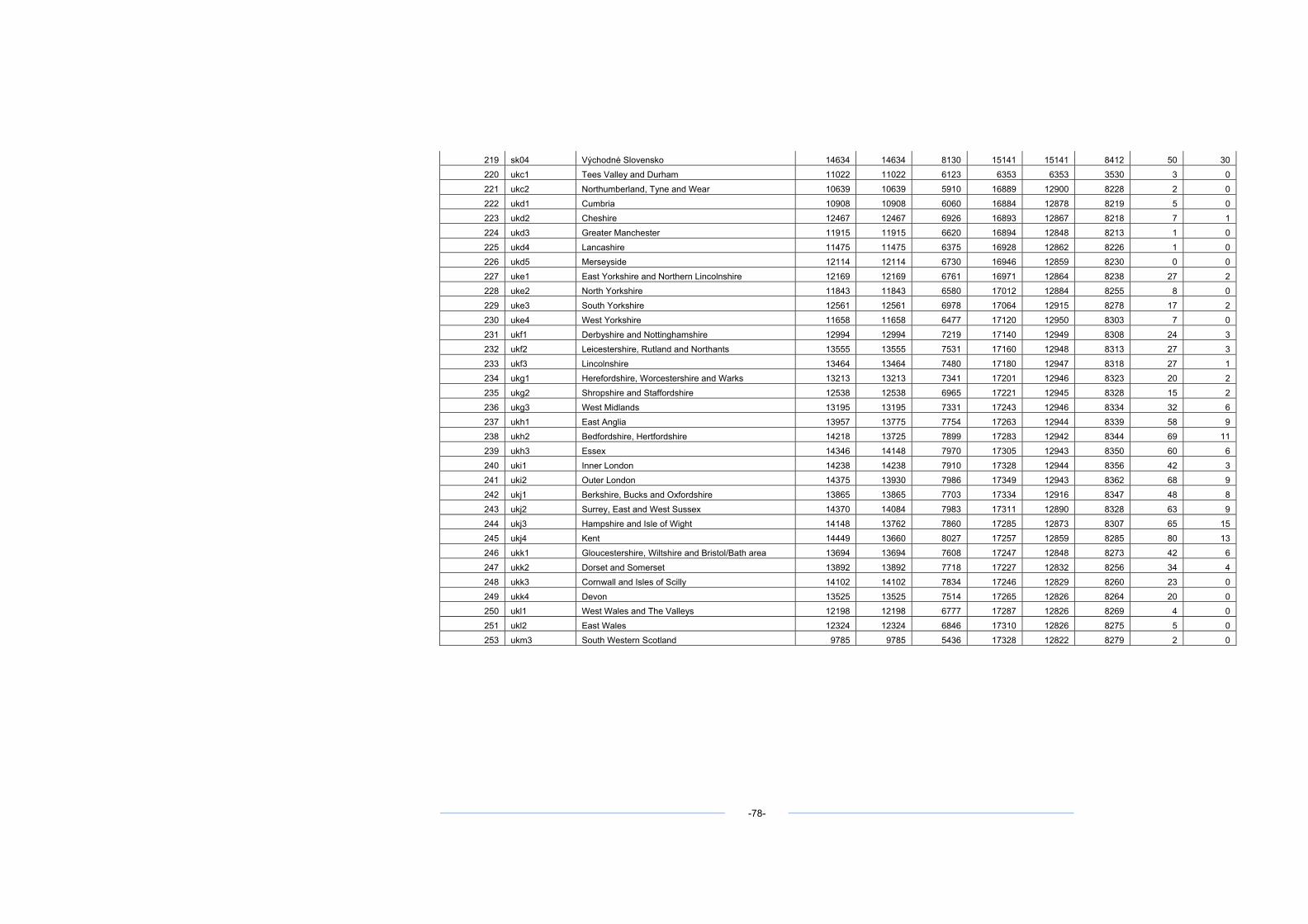
219 sk04 Východné Slovensko 14634 14634 8130 15141 15141 8412 50 30 220 ukc1 Tees Valley and Durham 11022 11022 6123 6353 6353 3530 3 0 221 ukc2 Northumberland, Tyne and Wear 10639 10639 5910 16889 12900 8228 2 0 222 ukd1 Cumbria 10908 10908 6060 16884 12878 8219 5 0 223 ukd2 Cheshire 12467 12467 6926 16893 12867 8218 7 1 224 ukd3 Greater Manchester 11915 11915 6620 16894 12848 8213 1 0 225 ukd4 Lancashire 11475 11475 6375 16928 12862 8226 1 0 226 ukd5 Merseyside 12114 12114 6730 16946 12859 8230 0 0 227 uke1 East Yorkshire and Northern Lincolnshire 12169 12169 6761 16971 12864 8238 27 2 228 uke2 North Yorkshire 11843 11843 6580 17012 12884 8255 8 0 229 uke3 South Yorkshire 12561 12561 6978 17064 12915 8278 17 2 230 uke4 West Yorkshire 11658 11658 6477 17120 12950 8303 7 0 231 ukf1 Derbyshire and Nottinghamshire 12994 12994 7219 17140 12949 8308 24 3 232 ukf2 Leicestershire, Rutland and Northants 13555 13555 7531 17160 12948 8313 27 3 233 ukf3 Lincolnshire 13464 13464 7480 17180 12947 8318 27 1 234 ukg1 Herefordshire, Worcestershire and Warks 13213 13213 7341 17201 12946 8323 20 2 235 ukg2 Shropshire and Staffordshire 12538 12538 6965 17221 12945 8328 15 2 236 ukg3 West Midlands 13195 13195 7331 17243 12946 8334 32 6 237 ukh1 East Anglia 13957 13775 7754 17263 12944 8339 58 9 238 ukh2 Bedfordshire, Hertfordshire 14218 13725 7899 17283 12942 8344 69 11 239 ukh3 Essex 14346 14148 7970 17305 12943 8350 60 6 240 uki1 Inner London 14238 14238 7910 17328 12944 8356 42 3 241 uki2 Outer London 14375 13930 7986 17349 12943 8362 68 9 242 ukj1 Berkshire, Bucks and Oxfordshire 13865 13865 7703 17334 12916 8347 48 8 243 ukj2 Surrey, East and West Sussex 14370 14084 7983 17311 12890 8328 63 9 244 ukj3 Hampshire and Isle of Wight 14148 13762 7860 17285 12873 8307 65 15 245 ukj4 Kent 14449 13660 8027 17257 12859 8285 80 13 246 ukk1 Gloucestershire, Wiltshire and Bristol/Bath area 13694 13694 7608 17247 12848 8273 42 6 247 ukk2 Dorset and Somerset 13892 13892 7718 17227 12832 8256 34 4 248 ukk3 Cornwall and Isles of Scilly 14102 14102 7834 17246 12829 8260 23 0 249 ukk4 Devon 13525 13525 7514 17265 12826 8264 20 0 250 ukl1 West Wales and The Valleys 12198 12198 6777 17287 12826 8269 4 0 251 ukl2 East Wales 12324 12324 6846 17310 12826 8275 5 0 253 ukm3 South Western Scotland 9785 9785 5436 17328 12822 8279 2 0

-78-

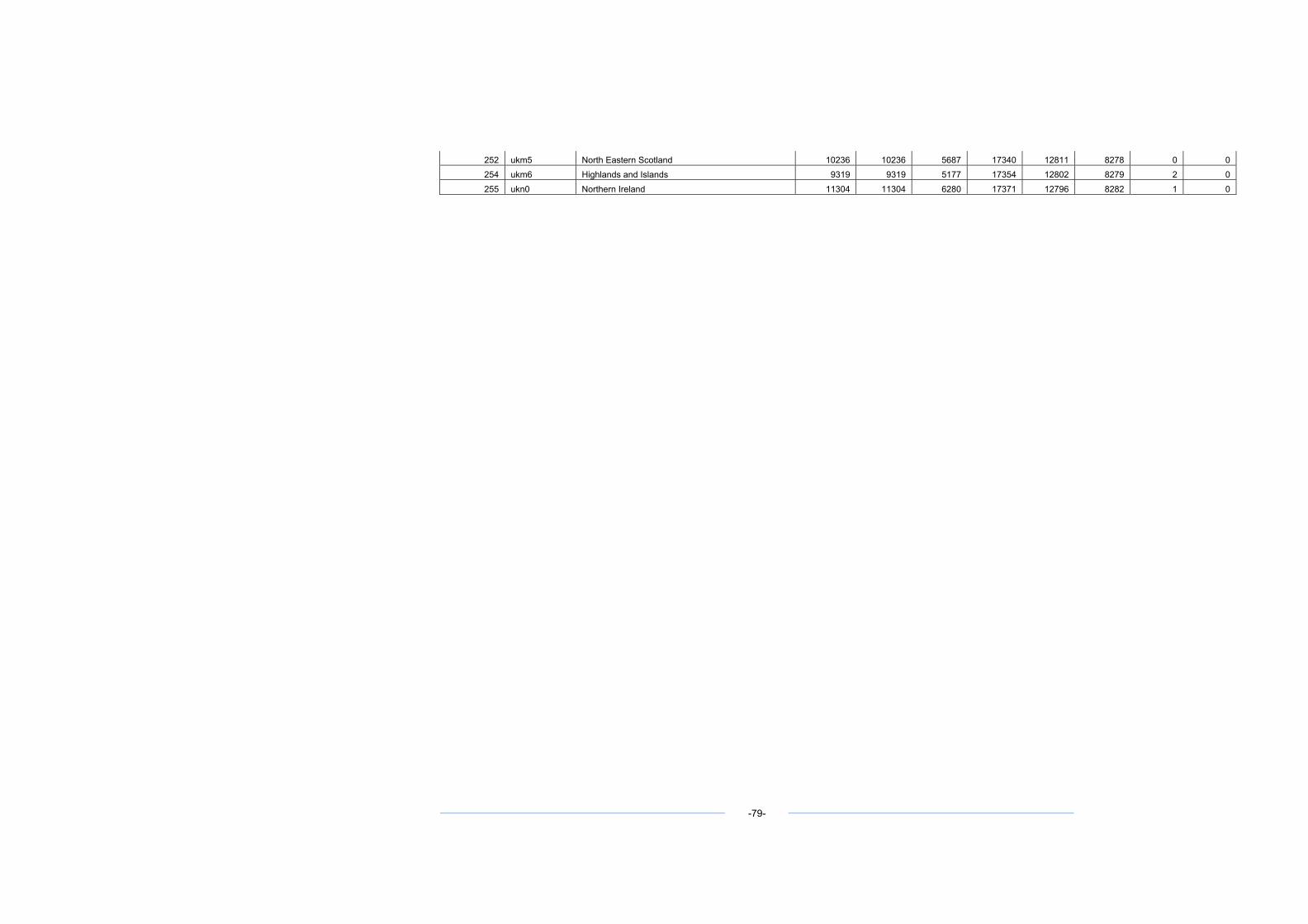
-79-

252 ukm5 North Eastern Scotland 10236 10236 5687 17340 12811 8278 0 0 254 ukm6 Highlands and Islands 9319 9319 5177 17354 12802 8279 2 0 255 ukn0 Northern Ireland 11304 11304 6280 17371 12796 8282 1 0

-80-

4. Implementation of 3 scenario/storyline specifications into qualitative estimates of irrigation water use, biomass and energy yield levels per RBD

Step 1: Estimation of land availability according to CAPSIM and desaggregation of land availability from national to regional (NUTS-2) level.

CAPSIM predicts the land need in 2020 for arable, set-aside-fallow, grasslands and permanent crops. By comparing the land use of these crop categories between 2000 and 2020 an estimate can be made of types of land released in these categories.

This then results into a potential land availability which needs to be translated further to an estimate of land that is likely to be converted to biomass cropping.

This is done by assuming the following detailed rules:

1. A proportion of 1% to 4% (depending on urbanization pressure per country (based on EEA (2007), Table 13) of the released land is removed from the potential to be used for non-agricultural purposes.

2. It is assumed that land released in the arable category has a higher chance to be converted to biomass cropping, than released set-aside/fallow land. To implement this 100% of the released arable land (after correction for non-agricultural uses) is expected to be converted and initially only 50% of the released set-aside/fallow land.

3. In countries for which statistical or published evidence is given of high passed land abandonment figures (based Pointereau et al., 2008) an extra 10% or 20% of released land (according to CAPSIM) is expected to be available for biomass cropping. This will only be the case for most CEEC countries and some Mediterranean countries. This land resource is added to the set-aside/fallow land pool.

4. For the latter categories, e.g. released set-aside/fallow and abandoned land, it could well be the case that even less of the 50% share is used depending on the initial crop mix assumed for every region. After all, the assumption is that perennials can grow on both good arable land and lower quality land in the set-aside/fallow land abandonment pool. But for the arable rotational crops the land quality requirements are higher. This means that if a large share of bioenergy crops is assumed to belong to this rotational type and this share cannot be fitted with the released arable land pool, the remainder cannot be automatically placed in the lower quality land pool. If this mis-match exist it leads to a reduction of land to become available for biomass cropping in a region. Because of this it will well be the case that less then 50% of the total land release is really going to be used (also depends on step 3).

5. The present (2006-2007) bioenergy cropping area is assumed to continue to be maintained in biomass cropping in 2020. This means that the present bioenergy cropping area should be added up with the released land resource as predicted by CAPSIM. Overall, this present bioenergy cropping area is seen as a land use that was mainly created under influence of national and regional stimulation policies which have not been taken into account in the CAPSIM scenario applications (CAPSIM assumes no stimulation policy for bioenergy). In practice many of these 2006/2007 bioenergy crops were also growing on set-aside land (at least in EU-15) for which the CAPSIM scenario only assumed a set-aside obligation and no active use for bioenergy through the 45 Euro per hectare non-food support. The assumption is however that this non-food support was not the (main) reason that farmers were growing the bioenergy crops, but rather other local stimulation and market opportunities made it attractive. In the future we assume that EU-national and regional governments and local markets remain giving enough stimulus to continue this cropping pattern. On

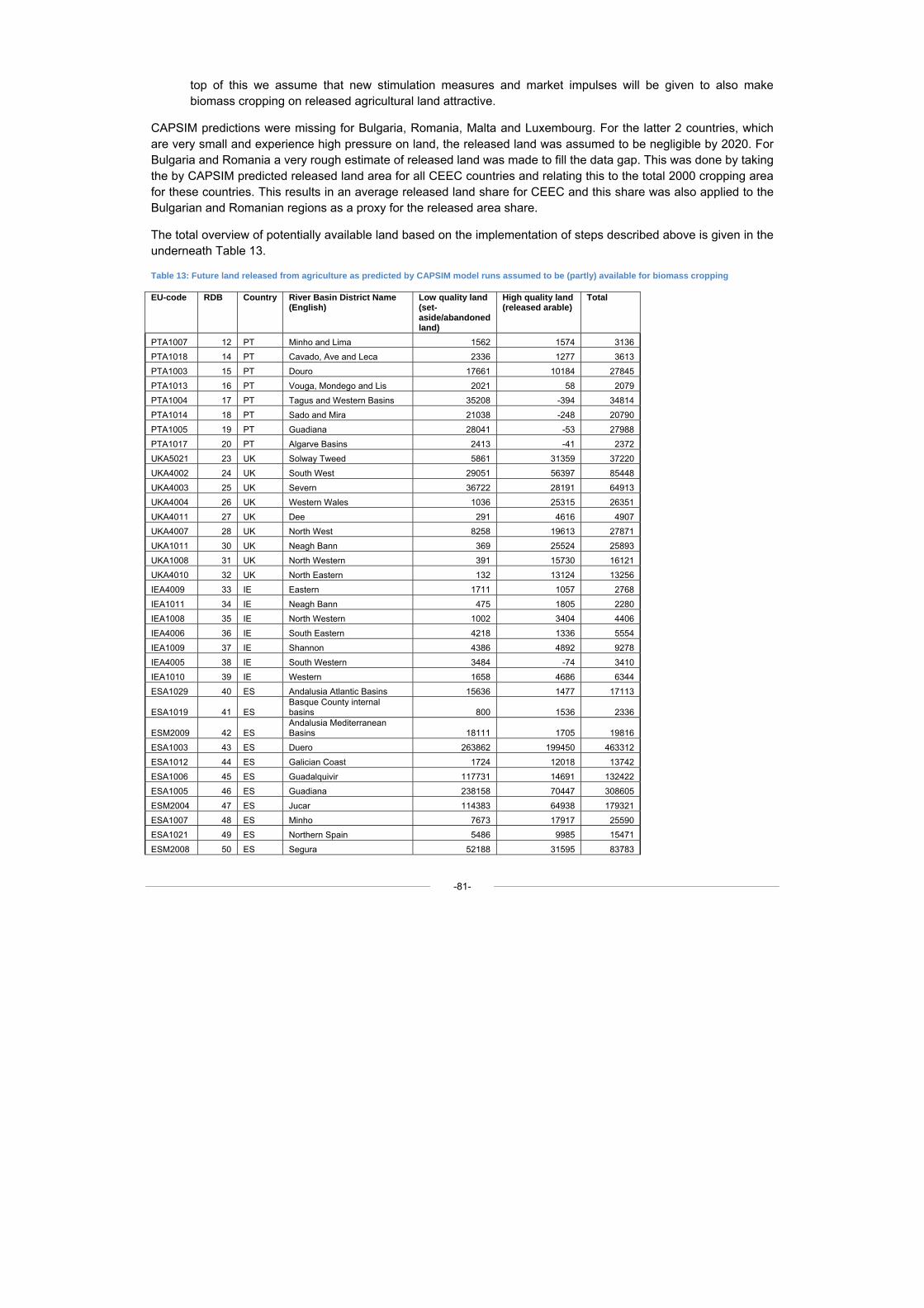
-81-

top of this we assume that new stimulation measures and market impulses will be given to also make biomass cropping on released agricultural land attractive.

CAPSIM predictions were missing for Bulgaria, Romania, Malta and Luxembourg. For the latter 2 countries, which are very small and experience high pressure on land, the released land was assumed to be negligible by 2020. For Bulgaria and Romania a very rough estimate of released land was made to fill the data gap. This was done by taking the by CAPSIM predicted released land area for all CEEC countries and relating this to the total 2000 cropping area for these countries. This results in an average released land share for CEEC and this share was also applied to the Bulgarian and Romanian regions as a proxy for the released area share.

The total overview of potentially available land based on the implementation of steps described above is given in the underneath Table 13.

Table 13: Future land released from agriculture as predicted by CAPSIM model runs assumed to be (partly) available for biomass cropping

EU-code RDB Country River Basin District Name (English)

Low quality land (set-aside/abandoned land)

High quality land (released arable)

Total

PTA1007 12 PT Minho and Lima 1562 1574 3136 PTA1018 14 PT Cavado, Ave and Leca 2336 1277 3613 PTA1003 15 PT Douro 17661 10184 27845 PTA1013 16 PT Vouga, Mondego and Lis 2021 58 2079 PTA1004 17 PT Tagus and Western Basins 35208 -394 34814 PTA1014 18 PT Sado and Mira 21038 -248 20790 PTA1005 19 PT Guadiana 28041 -53 27988 PTA1017 20 PT Algarve Basins 2413 -41 2372 UKA5021 23 UK Solway Tweed 5861 31359 37220 UKA4002 24 UK South West 29051 56397 85448 UKA4003 25 UK Severn 36722 28191 64913 UKA4004 26 UK Western Wales 1036 25315 26351 UKA4011 27 UK Dee 291 4616 4907 UKA4007 28 UK North West 8258 19613 27871 UKA1011 30 UK Neagh Bann 369 25524 25893 UKA1008 31 UK North Western 391 15730 16121 UKA4010 32 UK North Eastern 132 13124 13256 IEA4009 33 IE Eastern 1711 1057 2768 IEA1011 34 IE Neagh Bann 475 1805 2280 IEA1008 35 IE North Western 1002 3404 4406 IEA4006 36 IE South Eastern 4218 1336 5554 IEA1009 37 IE Shannon 4386 4892 9278 IEA4005 38 IE South Western 3484 -74 3410 IEA1010 39 IE Western 1658 4686 6344 ESA1029 40 ES Andalusia Atlantic Basins 15636 1477 17113

ESA1019 41 ES Basque County internal basins 800 1536 2336

ESM2009 42 ES Andalusia Mediterranean Basins 18111 1705 19816

ESA1003 43 ES Duero 263862 199450 463312 ESA1012 44 ES Galician Coast 1724 12018 13742 ESA1006 45 ES Guadalquivir 117731 14691 132422 ESA1005 46 ES Guadiana 238158 70447 308605 ESM2004 47 ES Jucar 114383 64938 179321 ESA1007 48 ES Minho 7673 17917 25590 ESA1021 49 ES Northern Spain 5486 9985 15471 ESM2008 50 ES Segura 52188 31595 83783

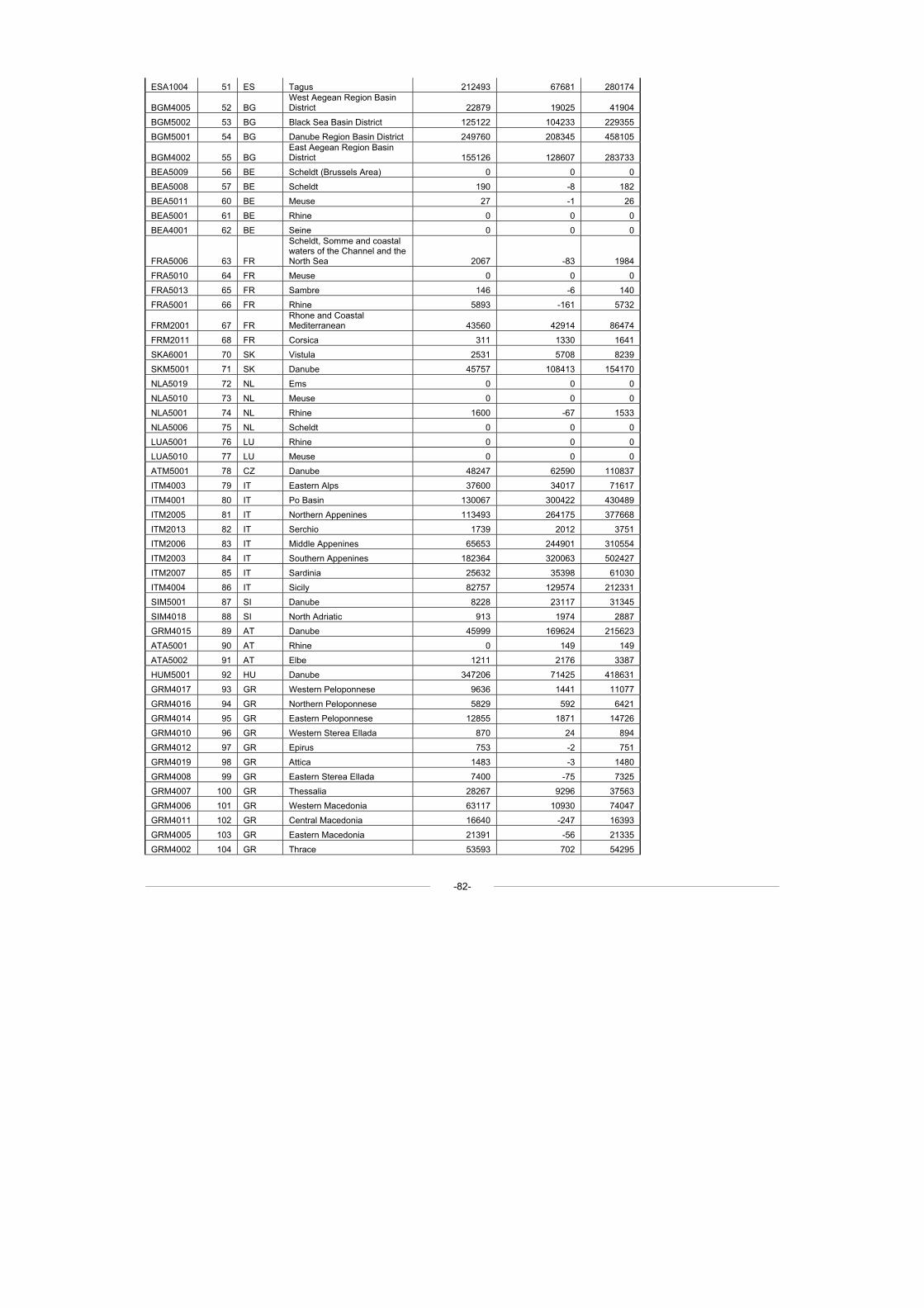
-82-

ESA1004 51 ES Tagus 212493 67681 280174

BGM4005 52 BG West Aegean Region Basin District 22879 19025 41904

BGM5002 53 BG Black Sea Basin District 125122 104233 229355 BGM5001 54 BG Danube Region Basin District 249760 208345 458105

BGM4002 55 BG East Aegean Region Basin District 155126 128607 283733

BEA5009 56 BE Scheldt (Brussels Area) 0 0 0 BEA5008 57 BE Scheldt 190 -8 182 BEA5011 60 BE Meuse 27 -1 26 BEA5001 61 BE Rhine 0 0 0 BEA4001 62 BE Seine 0 0 0

FRA5006 63 FR

Scheldt, Somme and coastal waters of the Channel and the North Sea 2067 -83 1984

FRA5010 64 FR Meuse 0 0 0 FRA5013 65 FR Sambre 146 -6 140 FRA5001 66 FR Rhine 5893 -161 5732

FRM2001 67 FR Rhone and Coastal Mediterranean 43560 42914 86474

FRM2011 68 FR Corsica 311 1330 1641 SKA6001 70 SK Vistula 2531 5708 8239 SKM5001 71 SK Danube 45757 108413 154170 NLA5019 72 NL Ems 0 0 0 NLA5010 73 NL Meuse 0 0 0 NLA5001 74 NL Rhine 1600 -67 1533 NLA5006 75 NL Scheldt 0 0 0 LUA5001 76 LU Rhine 0 0 0 LUA5010 77 LU Meuse 0 0 0 ATM5001 78 CZ Danube 48247 62590 110837 ITM4003 79 IT Eastern Alps 37600 34017 71617 ITM4001 80 IT Po Basin 130067 300422 430489 ITM2005 81 IT Northern Appenines 113493 264175 377668 ITM2013 82 IT Serchio 1739 2012 3751 ITM2006 83 IT Middle Appenines 65653 244901 310554 ITM2003 84 IT Southern Appenines 182364 320063 502427 ITM2007 85 IT Sardinia 25632 35398 61030 ITM4004 86 IT Sicily 82757 129574 212331 SIM5001 87 SI Danube 8228 23117 31345 SIM4018 88 SI North Adriatic 913 1974 2887 GRM4015 89 AT Danube 45999 169624 215623 ATA5001 90 AT Rhine 0 149 149 ATA5002 91 AT Elbe 1211 2176 3387 HUM5001 92 HU Danube 347206 71425 418631 GRM4017 93 GR Western Peloponnese 9636 1441 11077 GRM4016 94 GR Northern Peloponnese 5829 592 6421 GRM4014 95 GR Eastern Peloponnese 12855 1871 14726 GRM4010 96 GR Western Sterea Ellada 870 24 894 GRM4012 97 GR Epirus 753 -2 751 GRM4019 98 GR Attica 1483 -3 1480 GRM4008 99 GR Eastern Sterea Ellada 7400 -75 7325 GRM4007 100 GR Thessalia 28267 9296 37563 GRM4006 101 GR Western Macedonia 63117 10930 74047 GRM4011 102 GR Central Macedonia 16640 -247 16393 GRM4005 103 GR Eastern Macedonia 21391 -56 21335 GRM4002 104 GR Thrace 53593 702 54295

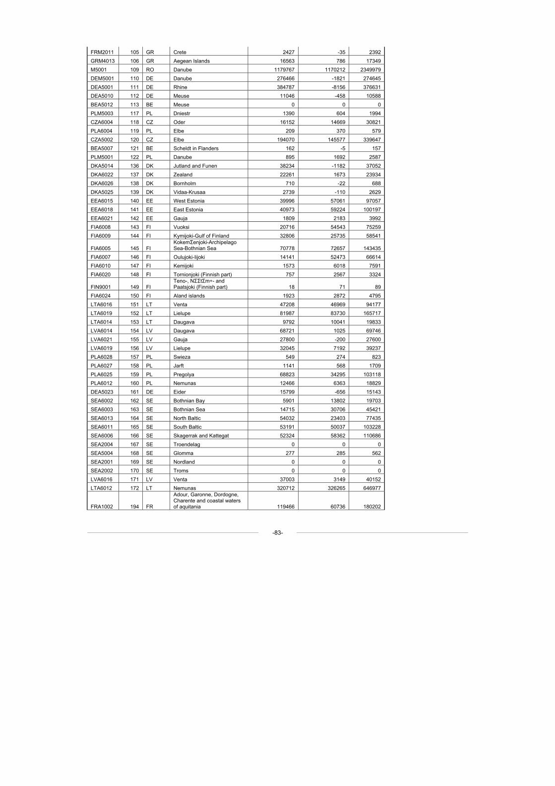
-83-

FRM2011 105 GR Crete 2427 -35 2392 GRM4013 106 GR Aegean Islands 16563 786 17349 M5001 109 RO Danube 1179767 1170212 2349979 DEM5001 110 DE Danube 276466 -1821 274645 DEA5001 111 DE Rhine 384787 -8156 376631 DEA5010 112 DE Meuse 11046 -458 10588 BEA5012 113 BE Meuse 0 0 0 PLM5003 117 PL Dniestr 1390 604 1994 CZA6004 118 CZ Oder 16152 14669 30821 PLA6004 119 PL Elbe 209 370 579 CZA5002 120 CZ Elbe 194070 145577 339647 BEA5007 121 BE Scheldt in Flanders 162 -5 157 PLM5001 122 PL Danube 895 1692 2587 DKA5014 136 DK Jutland and Funen 38234 -1182 37052 DKA6022 137 DK Zealand 22261 1673 23934 DKA6026 138 DK Bornholm 710 -22 688 DKA5025 139 DK Vidaa-Krusaa 2739 -110 2629 EEA6015 140 EE West Estonia 39996 57061 97057 EEA6018 141 EE East Estonia 40973 59224 100197 EEA6021 142 EE Gauja 1809 2183 3992 FIA6008 143 FI Vuoksi 20716 54543 75259 FIA6009 144 FI Kymijoki-Gulf of Finland 32806 25735 58541

FIA6005 145 FI KokemΣenjoki-Archipelago Sea-Bothnian Sea 70778 72657 143435

FIA6007 146 FI Oulujoki-Iijoki 14141 52473 66614 FIA6010 147 FI Kemijoki 1573 6018 7591 FIA6020 148 FI Tornionjoki (Finnish part) 757 2567 3324

FIN9001 149 FI Teno-, NΣΣtΣm÷- and Paatsjoki (Finnish part) 18 71 89

FIA6024 150 FI Aland islands 1923 2872 4795 LTA6016 151 LT Venta 47208 46969 94177 LTA6019 152 LT Lielupe 81987 83730 165717 LTA6014 153 LT Daugava 9792 10041 19833 LVA6014 154 LV Daugava 68721 1025 69746 LVA6021 155 LV Gauja 27800 -200 27600 LVA6019 156 LV Lielupe 32045 7192 39237 PLA6028 157 PL Swieza 549 274 823 PLA6027 158 PL Jarft 1141 568 1709 PLA6025 159 PL Pregolya 68823 34295 103118 PLA6012 160 PL Nemunas 12466 6363 18829 DEA5023 161 DE Eider 15799 -656 15143 SEA6002 162 SE Bothnian Bay 5901 13802 19703 SEA6003 163 SE Bothnian Sea 14715 30706 45421 SEA6013 164 SE North Baltic 54032 23403 77435 SEA6011 165 SE South Baltic 53191 50037 103228 SEA6006 166 SE Skagerrak and Kattegat 52324 58362 110686 SEA2004 167 SE Troendelag 0 0 0 SEA5004 168 SE Glomma 277 285 562 SEA2001 169 SE Nordland 0 0 0 SEA2002 170 SE Troms 0 0 0 LVA6016 171 LV Venta 37003 3149 40152 LTA6012 172 LT Nemunas 320712 326265 646977

FRA1002 194 FR

Adour, Garonne, Dordogne, Charente and coastal waters of aquitania 119466 60736 180202

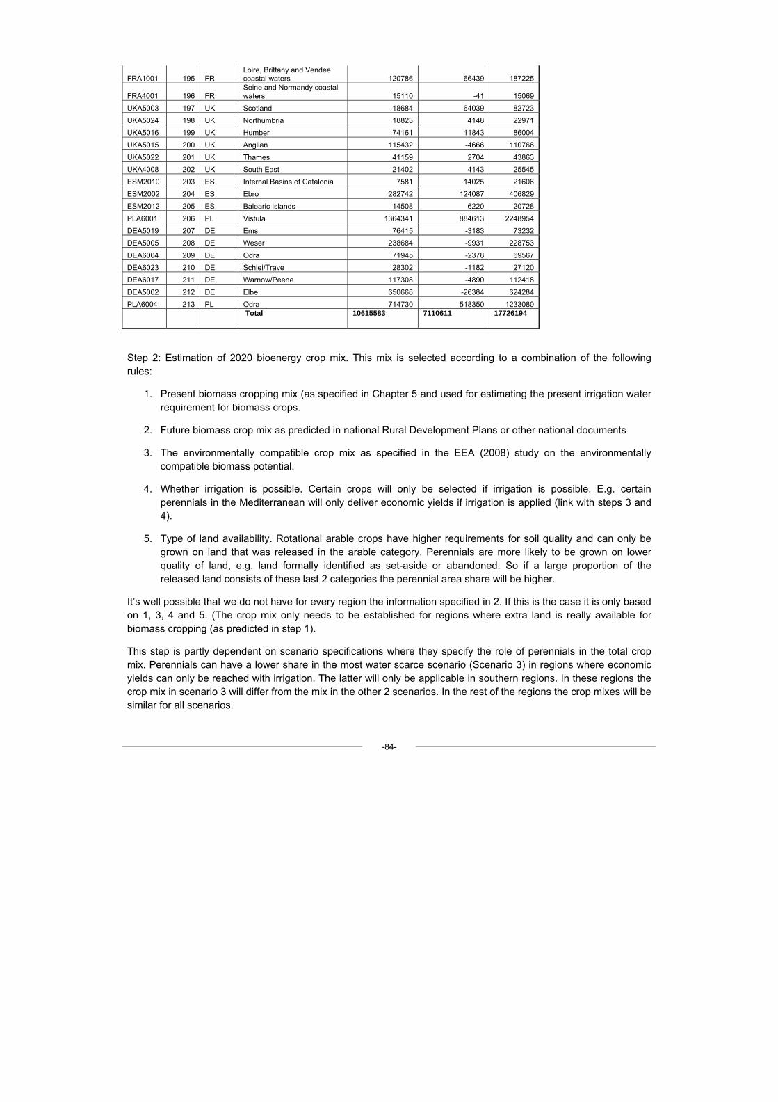
-84-

FRA1001 195 FR Loire, Brittany and Vendee coastal waters 120786 66439 187225

FRA4001 196 FR Seine and Normandy coastal waters 15110 -41 15069

UKA5003 197 UK Scotland 18684 64039 82723 UKA5024 198 UK Northumbria 18823 4148 22971 UKA5016 199 UK Humber 74161 11843 86004 UKA5015 200 UK Anglian 115432 -4666 110766 UKA5022 201 UK Thames 41159 2704 43863 UKA4008 202 UK South East 21402 4143 25545 ESM2010 203 ES Internal Basins of Catalonia 7581 14025 21606 ESM2002 204 ES Ebro 282742 124087 406829 ESM2012 205 ES Balearic Islands 14508 6220 20728 PLA6001 206 PL Vistula 1364341 884613 2248954 DEA5019 207 DE Ems 76415 -3183 73232 DEA5005 208 DE Weser 238684 -9931 228753 DEA6004 209 DE Odra 71945 -2378 69567 DEA6023 210 DE Schlei/Trave 28302 -1182 27120 DEA6017 211 DE Warnow/Peene 117308 -4890 112418 DEA5002 212 DE Elbe 650668 -26384 624284 PLA6004 213 PL Odra 714730 518350 1233080 Total 10615583 7110611 17726194

Step 2: Estimation of 2020 bioenergy crop mix. This mix is selected according to a combination of the following rules:

1. Present biomass cropping mix (as specified in Chapter 5 and used for estimating the present irrigation water requirement for biomass crops.

2. Future biomass crop mix as predicted in national Rural Development Plans or other national documents

3. The environmentally compatible crop mix as specified in the EEA (2008) study on the environmentally compatible biomass potential.

4. Whether irrigation is possible. Certain crops will only be selected if irrigation is possible. E.g. certain perennials in the Mediterranean will only deliver economic yields if irrigation is applied (link with steps 3 and 4).

5. Type of land availability. Rotational arable crops have higher requirements for soil quality and can only be grown on land that was released in the arable category. Perennials are more likely to be grown on lower quality of land, e.g. land formally identified as set-aside or abandoned. So if a large proportion of the released land consists of these last 2 categories the perennial area share will be higher.

It’s well possible that we do not have for every region the information specified in 2. If this is the case it is only based on 1, 3, 4 and 5. (The crop mix only needs to be established for regions where extra land is really available for biomass cropping (as predicted in step 1).

This step is partly dependent on scenario specifications where they specify the role of perennials in the total crop mix. Perennials can have a lower share in the most water scarce scenario (Scenario 3) in regions where economic yields can only be reached with irrigation. The latter will only be applicable in southern regions. In these regions the crop mix in scenario 3 will differ from the mix in the other 2 scenarios. In the rest of the regions the crop mixes will be similar for all scenarios.

-85-

Step 3: Distribute the total biomass crop mix (identified in step 2) over the total land area released per region (as predicted in step 1) and determine the final cropping area per biomass crop and region. In this step the final crop mix is determined per region, while in step 2 the average crop mix is still determined at the national level. In this step the overall crop mix is fitted to the production circumstances in a region and land quality. Crops that do not fit with the regional bio-climatic circumstances are not allocated to that region, even if they are part of the national bioenergy crop mix (determined in step 2). In addition, the crop mix is also fitted to the type (quality) of land released. Rotational arable crops can only be allocated to land released in the arable category (in step 1) and if this is not enough only a small part (up to 20%) of the released set-aside/fallow and abandoned land category. This is because it can only be assumed for a small part of this land that it has enough quality (or minor costs need to be made to make it suited) to be used for rotational cropping. So the final crop mix per region can turn out differently then the average national bioenergy crop mix.

Furthermore, because the mix does not always fit to the quality of released land it could well be that not all released land is really allocated to bioenergy cropping. This may often be the case as in many regions much more land is released in the set-aside/fallow abandonment category then in the arable category. This means that a large part of the rotational arable crop types cannot be allocated. This will then lead to a lower land allocation for bioenergy crops in that region and it will not lead to a complete shift in the cropping mix towards perennials in that region.

Step 4: Identification of the regions that are water scarce and the ones where additional irrigation water will be available for biomass cropping. Calculate per region (NUTS-2) the total amount of additional water availability, given scenario specifications, to be used for food and feed and for biomass cropping. And in the water scarce regions in the case of scenario 3, the amount of water that is no longer available for irrigation because of water saving measures.

Step 5: Identify per region whether there is room for irrigation of biomass crops and what amount of water can be used for these crops. It is assumed that in the RB where irrigation area can increase (specified per scenario) 1/3 of the water that becomes available can be used for biomass cropping. Distribute this total amount of water according to a weighting over the biomass crop mix specified already in step 2. The distribution of irrigation water available for biomass cropping should be distributed by taking account of the following rules/weighting:

1. Biomass crops will only be irrigated if this leads to a significantly higher yield in that typical location and/or if this crop can only deliver an economic yield in that location with irrigation (e.g. certain perennials in Mediterranean regions). Yield-water requirement levels are known per region/10*10 grid from the MARS-CGMS model-weather assessments for the most common rotational arable crops (see Annex 1 description). For the perennials separate crop growth modeling has been applied to determine the yield-water-requirement combinations per (15*15 km grid) for the whole of Europe under water limited and irrigated circumstances. From these calculations the practical yield-irrigation levels and yield levels under water limited conditions can be derived per grid/region.

2. Crops are only selected for irrigation if irrigation practice is already common in that region. Information about how common irrigation is for that crop in that region can be determined on the basis of irrigation crop shares in 2005 as predicted by Wriedt et al. (2008). For perennials this information is however not available.

3. A prioritization is determined according to which the irrigation water is distributed over the total biomass crop mix. High yielding (Tons DM/ha) and very water efficient crops (Liters/ton DM) get higher priority.

Step 6: Disaggregation of all calculated information from the region levels (NUTS-2) to the grid level in order to allocate the grid level information to RBD and make total calculations per RBD. This involves allocation to grid level of the following categories of information:

1. biomass cropping area per crop,

-86-

2. Irrigated area share per biomass crop

3. Yield level (tons Dry biomass) per biomass crop under water limited and irrigation condition (to calculate this see Section 3.3 and 3.4 in this Annex.

4. Translation of the yields in biomass to energy yield. For the conversion it was assumed that 1 kg of dry air biomass (15% water contents) equals 15 MJ energy.

Step 7: Mapping of information derived from Step 6 and calculate results at RBD level. This resulted in all mapped and tabled results presented in Chapter 6 and Annex 7:

Relative biomass cropping area (as % of total 2020 cropping area) per RBD in 2020 for 3 scenarios (3 maps, with same legend, try to make comparable to same map for 2007 situation (Map 1))

• Irrigated area share for biomass cropping (as percentage of total biomass cropping area) per RBD in 2020 for 3 scenarios

• Absolute irrigation water requirement for biomass cropping (in m3/year) in 2020 per RBD for 3 scenarios

• Relative irrigation share for biomass in total irrigation water requirement in 2020 per RBD for 3 scenarios

• Total biomass yield (tons Dry biomass) in 2020 per RBD for 3 scenarios

• Total biomass energy yield (in MJ/year) in 2020 per RBD for 3 scenarios (3 maps, with same legend)

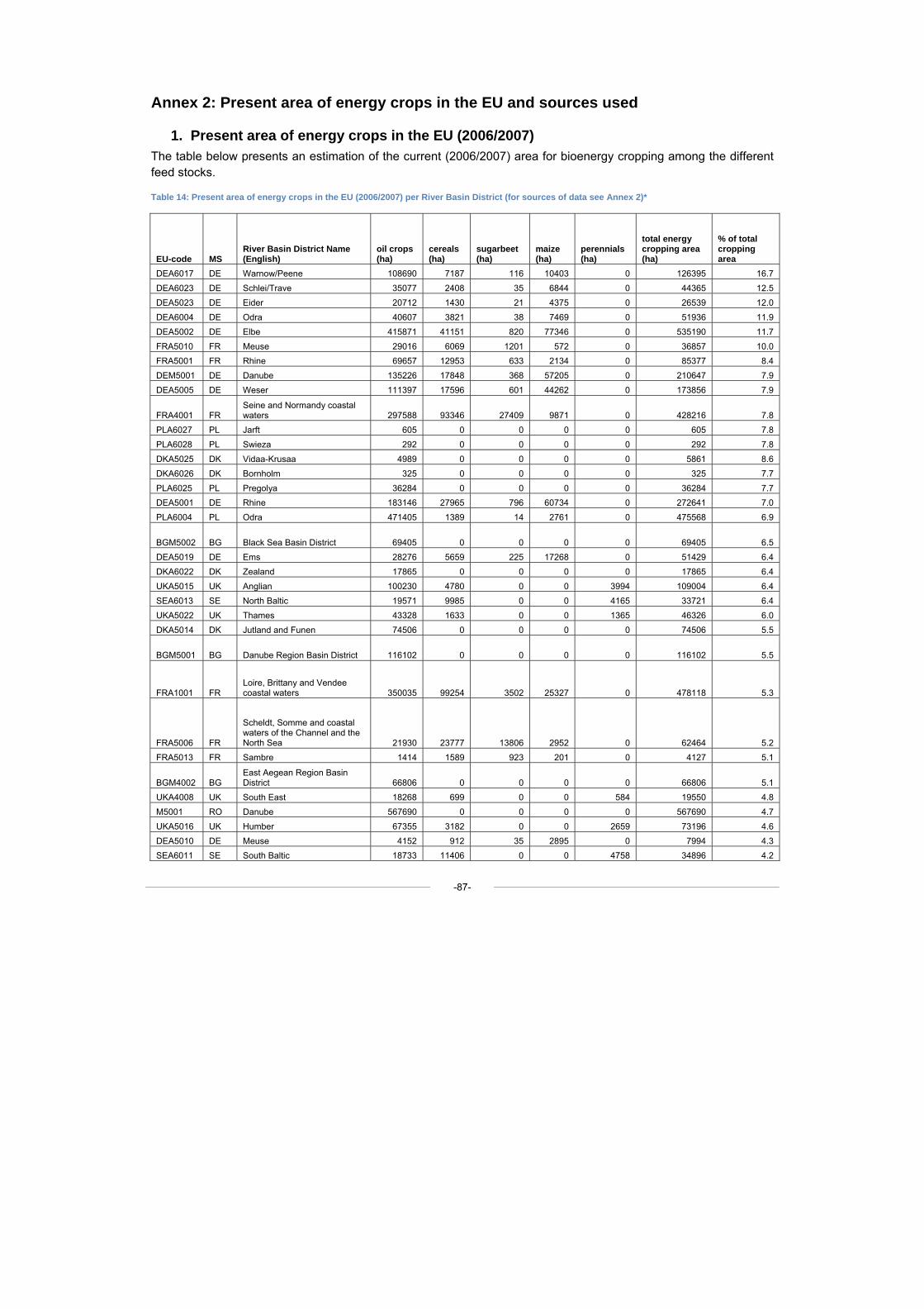
-87-

Annex 2: Present area of energy crops in the EU and sources used

1. Present area of energy crops in the EU (2006/2007) The table below presents an estimation of the current (2006/2007) area for bioenergy cropping among the different feed stocks.

Table 14: Present area of energy crops in the EU (2006/2007) per River Basin District (for sources of data see Annex 2)*

EU-code MS River Basin District Name (English)

oil crops (ha)

cereals (ha)

sugarbeet (ha)

maize (ha)

perennials (ha)

total energy cropping area (ha)

% of total cropping area

DEA6017 DE Warnow/Peene 108690 7187 116 10403 0 126395 16.7 DEA6023 DE Schlei/Trave 35077 2408 35 6844 0 44365 12.5 DEA5023 DE Eider 20712 1430 21 4375 0 26539 12.0 DEA6004 DE Odra 40607 3821 38 7469 0 51936 11.9 DEA5002 DE Elbe 415871 41151 820 77346 0 535190 11.7 FRA5010 FR Meuse 29016 6069 1201 572 0 36857 10.0 FRA5001 FR Rhine 69657 12953 633 2134 0 85377 8.4 DEM5001 DE Danube 135226 17848 368 57205 0 210647 7.9 DEA5005 DE Weser 111397 17596 601 44262 0 173856 7.9

FRA4001 FR Seine and Normandy coastal waters 297588 93346 27409 9871 0 428216 7.8

PLA6027 PL Jarft 605 0 0 0 0 605 7.8 PLA6028 PL Swieza 292 0 0 0 0 292 7.8 DKA5025 DK Vidaa-Krusaa 4989 0 0 0 0 5861 8.6 DKA6026 DK Bornholm 325 0 0 0 0 325 7.7 PLA6025 PL Pregolya 36284 0 0 0 0 36284 7.7 DEA5001 DE Rhine 183146 27965 796 60734 0 272641 7.0 PLA6004 PL Odra 471405 1389 14 2761 0 475568 6.9

BGM5002 BG Black Sea Basin District 69405 0 0 0 0 69405 6.5 DEA5019 DE Ems 28276 5659 225 17268 0 51429 6.4 DKA6022 DK Zealand 17865 0 0 0 0 17865 6.4 UKA5015 UK Anglian 100230 4780 0 0 3994 109004 6.4 SEA6013 SE North Baltic 19571 9985 0 0 4165 33721 6.4 UKA5022 UK Thames 43328 1633 0 0 1365 46326 6.0 DKA5014 DK Jutland and Funen 74506 0 0 0 0 74506 5.5

BGM5001 BG Danube Region Basin District 116102 0 0 0 0 116102 5.5

FRA1001 FR Loire, Brittany and Vendee coastal waters 350035 99254 3502 25327 0 478118 5.3

FRA5006 FR

Scheldt, Somme and coastal waters of the Channel and the North Sea 21930 23777 13806 2952 0 62464 5.2

FRA5013 FR Sambre 1414 1589 923 201 0 4127 5.1

BGM4002 BG East Aegean Region Basin District 66806 0 0 0 0 66806 5.1

UKA4008 UK South East 18268 699 0 0 584 19550 4.8 M5001 RO Danube 567690 0 0 0 0 567690 4.7 UKA5016 UK Humber 67355 3182 0 0 2659 73196 4.6 DEA5010 DE Meuse 4152 912 35 2895 0 7994 4.3 SEA6011 SE South Baltic 18733 11406 0 0 4758 34896 4.2

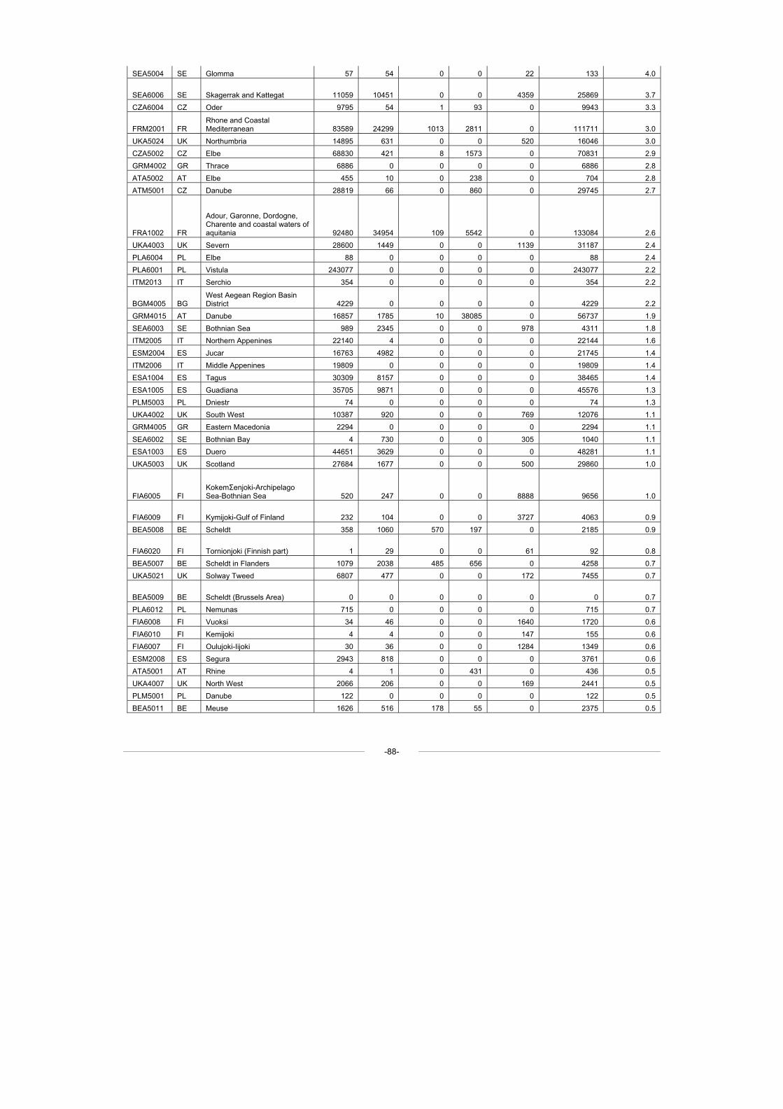
-88-

SEA5004 SE Glomma 57 54 0 0 22 133 4.0

SEA6006 SE Skagerrak and Kattegat 11059 10451 0 0 4359 25869 3.7 CZA6004 CZ Oder 9795 54 1 93 0 9943 3.3

FRM2001 FR Rhone and Coastal Mediterranean 83589 24299 1013 2811 0 111711 3.0

UKA5024 UK Northumbria 14895 631 0 0 520 16046 3.0 CZA5002 CZ Elbe 68830 421 8 1573 0 70831 2.9 GRM4002 GR Thrace 6886 0 0 0 0 6886 2.8 ATA5002 AT Elbe 455 10 0 238 0 704 2.8 ATM5001 CZ Danube 28819 66 0 860 0 29745 2.7

FRA1002 FR

Adour, Garonne, Dordogne, Charente and coastal waters of aquitania 92480 34954 109 5542 0 133084 2.6

UKA4003 UK Severn 28600 1449 0 0 1139 31187 2.4 PLA6004 PL Elbe 88 0 0 0 0 88 2.4 PLA6001 PL Vistula 243077 0 0 0 0 243077 2.2 ITM2013 IT Serchio 354 0 0 0 0 354 2.2

BGM4005 BG West Aegean Region Basin District 4229 0 0 0 0 4229 2.2

GRM4015 AT Danube 16857 1785 10 38085 0 56737 1.9 SEA6003 SE Bothnian Sea 989 2345 0 0 978 4311 1.8 ITM2005 IT Northern Appenines 22140 4 0 0 0 22144 1.6 ESM2004 ES Jucar 16763 4982 0 0 0 21745 1.4 ITM2006 IT Middle Appenines 19809 0 0 0 0 19809 1.4 ESA1004 ES Tagus 30309 8157 0 0 0 38465 1.4 ESA1005 ES Guadiana 35705 9871 0 0 0 45576 1.3 PLM5003 PL Dniestr 74 0 0 0 0 74 1.3 UKA4002 UK South West 10387 920 0 0 769 12076 1.1 GRM4005 GR Eastern Macedonia 2294 0 0 0 0 2294 1.1 SEA6002 SE Bothnian Bay 4 730 0 0 305 1040 1.1 ESA1003 ES Duero 44651 3629 0 0 0 48281 1.1 UKA5003 UK Scotland 27684 1677 0 0 500 29860 1.0

FIA6005 FI KokemΣenjoki-Archipelago Sea-Bothnian Sea 520 247 0 0 8888 9656 1.0

FIA6009 FI Kymijoki-Gulf of Finland 232 104 0 0 3727 4063 0.9

BEA5008 BE Scheldt 358 1060 570 197 0 2185 0.9

FIA6020 FI Tornionjoki (Finnish part) 1 29 0 0 61 92 0.8 BEA5007 BE Scheldt in Flanders 1079 2038 485 656 0 4258 0.7 UKA5021 UK Solway Tweed 6807 477 0 0 172 7455 0.7

BEA5009 BE Scheldt (Brussels Area) 0 0 0 0 0 0 0.7 PLA6012 PL Nemunas 715 0 0 0 0 715 0.7 FIA6008 FI Vuoksi 34 46 0 0 1640 1720 0.6 FIA6010 FI Kemijoki 4 4 0 0 147 155 0.6 FIA6007 FI Oulujoki-Iijoki 30 36 0 0 1284 1349 0.6 ESM2008 ES Segura 2943 818 0 0 0 3761 0.6 ATA5001 AT Rhine 4 1 0 431 0 436 0.5 UKA4007 UK North West 2066 206 0 0 169 2441 0.5 PLM5001 PL Danube 122 0 0 0 0 122 0.5 BEA5011 BE Meuse 1626 516 178 55 0 2375 0.5

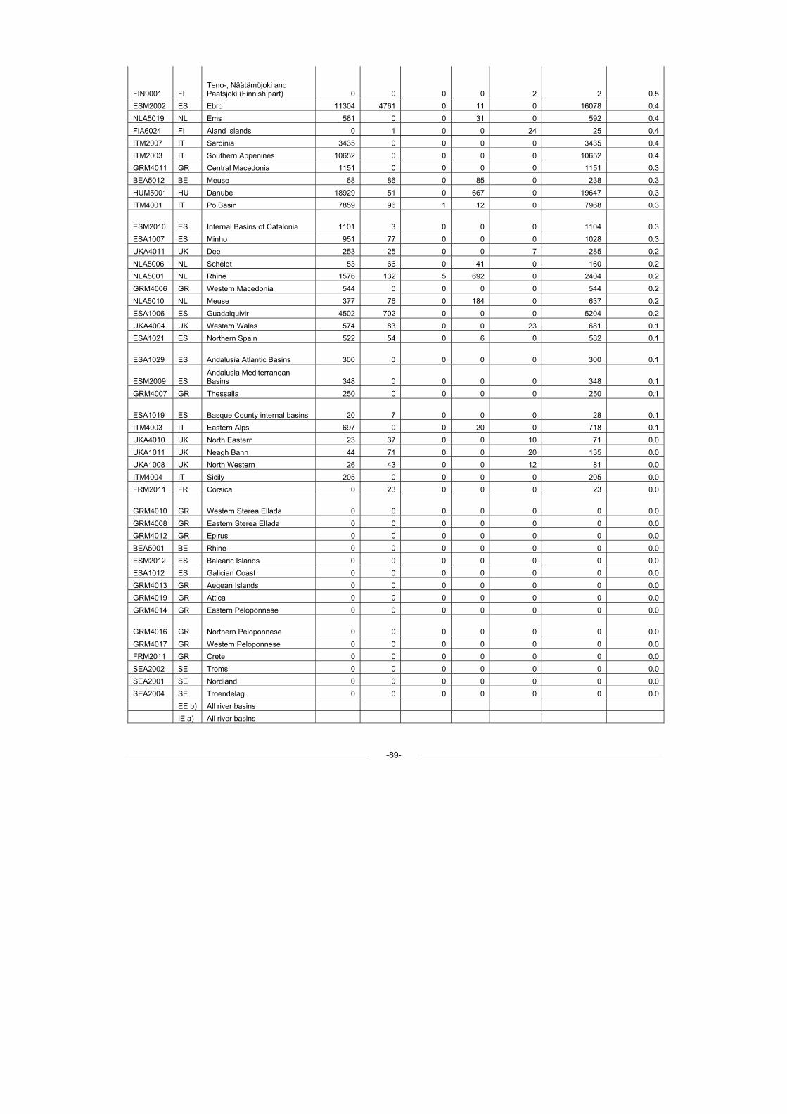
-89-

FIN9001 FI Teno-, Näätämöjoki and Paatsjoki (Finnish part) 0 0 0 0 2 2 0.5

ESM2002 ES Ebro 11304 4761 0 11 0 16078 0.4 NLA5019 NL Ems 561 0 0 31 0 592 0.4 FIA6024 FI Aland islands 0 1 0 0 24 25 0.4 ITM2007 IT Sardinia 3435 0 0 0 0 3435 0.4 ITM2003 IT Southern Appenines 10652 0 0 0 0 10652 0.4 GRM4011 GR Central Macedonia 1151 0 0 0 0 1151 0.3 BEA5012 BE Meuse 68 86 0 85 0 238 0.3 HUM5001 HU Danube 18929 51 0 667 0 19647 0.3 ITM4001 IT Po Basin 7859 96 1 12 0 7968 0.3

ESM2010 ES Internal Basins of Catalonia 1101 3 0 0 0 1104 0.3 ESA1007 ES Minho 951 77 0 0 0 1028 0.3 UKA4011 UK Dee 253 25 0 0 7 285 0.2 NLA5006 NL Scheldt 53 66 0 41 0 160 0.2 NLA5001 NL Rhine 1576 132 5 692 0 2404 0.2 GRM4006 GR Western Macedonia 544 0 0 0 0 544 0.2 NLA5010 NL Meuse 377 76 0 184 0 637 0.2 ESA1006 ES Guadalquivir 4502 702 0 0 0 5204 0.2 UKA4004 UK Western Wales 574 83 0 0 23 681 0.1 ESA1021 ES Northern Spain 522 54 0 6 0 582 0.1

ESA1029 ES Andalusia Atlantic Basins 300 0 0 0 0 300 0.1

ESM2009 ES Andalusia Mediterranean Basins 348 0 0 0 0 348 0.1

GRM4007 GR Thessalia 250 0 0 0 0 250 0.1

ESA1019 ES Basque County internal basins 20 7 0 0 0 28 0.1 ITM4003 IT Eastern Alps 697 0 0 20 0 718 0.1 UKA4010 UK North Eastern 23 37 0 0 10 71 0.0 UKA1011 UK Neagh Bann 44 71 0 0 20 135 0.0 UKA1008 UK North Western 26 43 0 0 12 81 0.0 ITM4004 IT Sicily 205 0 0 0 0 205 0.0 FRM2011 FR Corsica 0 23 0 0 0 23 0.0

GRM4010 GR Western Sterea Ellada 0 0 0 0 0 0 0.0

GRM4008 GR Eastern Sterea Ellada 0 0 0 0 0 0 0.0 GRM4012 GR Epirus 0 0 0 0 0 0 0.0 BEA5001 BE Rhine 0 0 0 0 0 0 0.0 ESM2012 ES Balearic Islands 0 0 0 0 0 0 0.0 ESA1012 ES Galician Coast 0 0 0 0 0 0 0.0 GRM4013 GR Aegean Islands 0 0 0 0 0 0 0.0 GRM4019 GR Attica 0 0 0 0 0 0 0.0 GRM4014 GR Eastern Peloponnese 0 0 0 0 0 0 0.0

GRM4016 GR Northern Peloponnese 0 0 0 0 0 0 0.0

GRM4017 GR Western Peloponnese 0 0 0 0 0 0 0.0 FRM2011 GR Crete 0 0 0 0 0 0 0.0 SEA2002 SE Troms 0 0 0 0 0 0 0.0 SEA2001 SE Nordland 0 0 0 0 0 0 0.0 SEA2004 SE Troendelag 0 0 0 0 0 0 0.0 EE b) All river basins IE a) All river basins

-90-

LT b) All river basins LV b) All river basins LU a) All river basins PT a) All river basins SI b) All river basins Total EU-27 4453290 515054 52988 385994 42304 5449636 3.2

a) MS where bioenergy cropping is currently not relevant b) MS where data on bioenergy cropping is missing * The original data for this table was mainly collected at national level (except for Spain and UK where some NUTS-2 level information was available). The distribution over River basins was done by using the present croping area (of relevant crops also used for bioenergy purposes, e.g. rape, sunflower, cereals, sugarbeet and maize) per NUTS/Riverbasin combination as a distribution factor. For further information on original sources see Annex 2.

2. Sources

Austria

Bioenergy production in 2006 (Brainbows Informationsmanagement GmbH (2007) and Raab (2007)):

• SRC (Miscanthus und others): some 100 ha

• Cereals for heating: more than 1,500 ha

• Biogas (Silage Maize and fodder: around 40,000 ha

• Bioethanol: no production ha

• Rape seed (biodiesel): about 15,000 ha

Belgium (only Flanders)

Information was received from Linda Meiresonne working for the Linda Research Institute for Nature and Forest. The underneath figures were derived from the Ministry of Agriculture. Arable crops: inventory based on applications for energy subsidy (45 €/ha) or set aside subsidy.

-91-

Energy – Situation 2007:

• Rapeseed: 507 ha

• Wheat: 200 ha

• Mais: 521 ha

Energy – Situation 2008:


• Mais: 508 ha

Set aside – Situation 2007:


• Wheat: 1,164 ha

• Mais: 139 ha

• Tricale: 2 ha

The Flemish region had 622,133 ha of agricultural land in 2007 (normal arable land and set-aside). So 0.45% of the agricultural area was occupied with targeted energy crops.

Bulgaria

A rough indication on oil cropping area for biodiesel purposes were derived from a European Biodiesel Board (EEB) report.

In this report it is stated biodiesel production first started in Bulgaria as early as 2001, and was mainly based on used cooking oils collected from restaurants, as developed by the company SAMPO in Brussartzi (North-Western Bulgaria). However, there has been a rapid increase in production of sunflower and rapeseed-based biodiesel. Today indeed, the energy crops used as raw material for biodiesel are mainly rapeseed and sunflower, although it should be noted that some climatic restrictions exist for rapeseed cultivation’ (Garofalo, 2007).

Based on this statement the present area of rape and oil seeds was taken from the FSS 2007 and then it was assumed that 1/3 of the production coming from this area was used for biodiesel production.

This leads to the following cropping area:

• Oil seed rape: 335 ha

• Sunflower: 257,759 ha

• Total: 258,094 ha

Cyprus

-92-

The hectares in agriculture used for bioenergy cropping in Cyprus is zero. In general the main reasons for not having such a RES in Cyprus is a) the requirements in high level technological knowledge (planning of installation, treatment of raw material). b) Lack of previous experience, c) Increased water requirement of energy crops in relation to the water stressed agriculture (Personal communication Ayis I. Iacovides).

Denmark:

Information on the cropping area was derived the Danish Ministry of Food, Agriculture and Fisheries, which specifies a total area of 95,000 hectares of oil seed rape. Leppiman (2005) also specifies that in Denmark biomass (mainly straw, wood and manure) accounts for nearly 10 % of the total energy production.

Estonia

Today energy crops (mainly Rapeseed) are grown within an area that does not exceed 50 thousand hectares. The harvest is about 70 – 80 thousand tonnes, which is not sufficient to produce biodiesel. Cereal production (approximately 600-760 thousand tonnes) does not currently cover domestic demand for fodder, foodstuff, seed and industrial needs. Therefore additional cereal is being imported to cover demand (not for conversion into ethanol)(Barz and Ahlhaus, 2005).

France

Until 2005 bioethanol in France was produced primarily from sugarbeet and secondarily from wheat: most bioethanol production is likely to be derived from wheat in 2008, at the expense of sugarbeet. According to the French Ministry of Agriculture, 300,000 hectares of wheat, 50,000 hectares of corn and 50,000 hectares of sugar beet are expected to produce bioethanol by 2008. For wheat and corn, this will represent less than 5% of the total grain acreage (Hénard and Audran, 2007).

France: Situation 2007/2008:

• OSR: 872,352 ha

• Sunflower: 80,000 ha

• Corn maize: 50,000 ha

• Starch (cereals): 300,000 ha

• Sugerbeet: 50,000 ha

• Total: 1,352,352 ha

Germany

There is significant increase in biomass cultivation for bioenergy purpose in Germany. The biggest production is focused on biodiesel. The oil seed crop cover already over 1,100,000 hectares, which is almost 10% of the arable land (Figure 3). Germany as a large central European country has 11.8 mill. hectares of arable land. Future biomass potentials in Germany for energy crops are stipulated to be even up to 2 mill. hectares or 17% of the arable land on medium to long terms.

Rapid growth in interest in biogas has been noticed recently in Germany. Between 2004 and 2005 the area dedicated for biogas energy crops increased over six times. Around 80% of the applied crops is maize, harvested for maize silage. Further growth is expected. In 2007 Germany had the highest number of biogas plants in Europe (around 3000). Biogas is produced from manure, industrial organic waste but especially from cultivated energy crops. Energy crops state for over 46% of the substrates. Share of animal manure is around 24% of feedstock

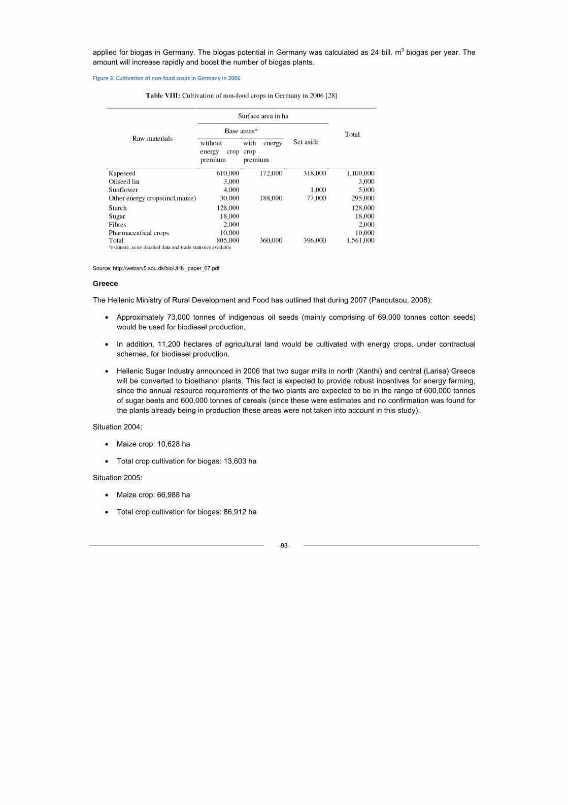
applied for biogas in Germany. The biogas potential in Germany was calculated as 24 bill. m3 biogas per year. The amount will increase rapidly and boost the number of biogas plants.

Figure 3: Cultivation of non-food crops in Germany in 2006

Source: http://websrv5.sdu.dk/bio/JHN_paper_07.pdf

Greece

The Hellenic Ministry of Rural Development and Food has outlined that during 2007 (Panoutsou, 2008):

• Approximately 73,000 tonnes of indigenous oil seeds (mainly comprising of 69,000 tonnes cotton seeds) would be used for biodiesel production,

• In addition, 11,200 hectares of agricultural land would be cultivated with energy crops, under contractual schemes, for biodiesel production.

• Hellenic Sugar Industry announced in 2006 that two sugar mills in north (Xanthi) and central (Larisa) Greece will be converted to bioethanol plants. This fact is expected to provide robust incentives for energy farming, since the annual resource requirements of the two plants are expected to be in the range of 600,000 tonnes of sugar beets and 600,000 tonnes of cereals (since these were estimates and no confirmation was found for the plants already being in production these areas were not taken into account in this study).

Situation 2004:

• Maize crop: 10,628 ha

• Total crop cultivation for biogas: 13,603 ha

Situation 2005:

• Maize crop: 66,988 ha

• Total crop cultivation for biogas: 86,912 ha

-93-

-94-

Hungary

In Hungary on 18,500 hectares energy crops were grown in 2008 (Doran, 2008).

Ireland

At present, biomass provides over half of Ireland's renewable energy - mainly through wood used for heating in the domestic and wood processing industry sectors (Bruton and McDermott, 2006).

Italy

Biodiesel in Italy is mainly produced from rapeseed oil (about 70% of the total) and soybean oil (20%), with the remainder coming from both sun and palm oils. Rapeseed oil is imported from other EU countries, while soybean oil is either imported from the EU or domestically produced from imported beans (oil from domestic beans, being GM free, is used for food consumption). According to industry sources, this year (2007) some 65,000 hectares have been or will be planted to oilseeds (50,000 hectares to sunflower seeds and 15,000 hectares to rapeseeds) under cultivation contracts between growers and the processing industry for the production of biodiesel. In 2006 bioethanol production rose to 1,280,000 hectoliters, obtained from alcohol produced from both the distillation of wine surpluses and molasses (Perini, 2007).

Poland

With plantations of about 2,000 hectares (2006) willows are mostly used as energy crop. Secondly, straw is becoming more popular for energy use, but it is currently only marginal in relation to overall production. Poland has set a target for expanding the area used for energy crops up to 160-200 thousand hectares in 2010 representing 1.2 – 1.4% of whole arable land in Poland. It may be an alternative sources of income for farmers. Now cultivation area of energetic willow is only 5.4 thousand hectares (Wesolowski, 2005).

Portugal

9,000 hectares area under energy crops in 2008 (Doran, 2008)

Romania

Romania has a significant potential for production of bioethanol from sweet sorghum and biodiesel from rape oil and sunflower oil. It also has very good prospects as a net exporter within the EU. In Romania, in 2004, almost all of 100,000 tonnes of rapeseed, 70,000 tonnes of sunflower and 408,000 tonnes of sunflower seeds were exported possibly for bioenergy production (Kondilia and Kaldellis, 2007).

UK

Final data used were derived from www.nnfcc.co.uk (National non-food crops website). The data on this website specify the following (in hectares):

England:

• SRC-willow: 3,083 ha

• SRC-poplar: 5 ha

• Miscanthus: 5,772 ha

Wales:

http://www.nnfcc.co.uk/

-95-

• SRC-willow: 7 ha

Scotland:


N-Ireland:


UK (region unknown):



Total:

• OSR: 320,542 ha

• Wheat; 14,614 ha

• Barley: 1,303 ha


• SRC-poplar: 5 ha


In addition other information was also provided on: http://www.rcep.org.uk/biomass/chapter2.pdf

It specified that willow (Salix spp.) has already been used in commercial or near commercial operations in the UK. Investment in developing new varieties with increased yield stability and improved crop management has made willow increasingly competitive as an energy source. Willow chips are a reliable source of fuel of a consistent quality, suitable for firing in CHP and district heating plants. Willow has been grown extensively in Scandinavia for fuel, and in Sweden some 15,000 hectares of land are dedicated to its production for renewable energy. Consequently, much more information about cultivation, harvesting and yields is available for willow than for the other potential energy crops.

The grass miscanthus (Miscanthus spp.) is attracting an increasing amount of interest but it is still largely at trial stage in the UK. Among other potential candidate species, poplar (Populus spp.) is closest to providing an alternative source of fuel. Poplar is being trialled in short rotation coppice (SRC) plantations, as well as being tried in silvoarable agro-forestry where it is intercropped with arable species.

There are currently 1,795 hectares of land under cultivation of commercial willow SRC and miscanthus in the UK; at least 1,500 hectares of this is willow. The land dedicated to energy crops totals less than 0.01% of the total arable land in the UK. The Defra Non- Food Crops Strategy states that domestically grown crops should meet a significant part of the demand for energy and raw materials in the UK. The National Farmers’ Union suggests that up to 20% of crops grown in the UK could be made available for non-food uses (i.e. for fuels or industrial materials), by 2020; hence, there is scope for a significant expansion of energy crop production in the UK. Planning crops in order to

http://www.rcep.org.uk/biomass/chapter2.pdf

-96-

achieve the maximum environmental benefits and yields in areas close to demand is the challenge to be met by the farmers and energy generating companies.

http://www.defra.gov.uk/farm/crops/industrial/research/reports/biofuels_prospects.pdf

In 2001, over 23,000 hectares of oilseed rape was grown on UK farms for biodiesel production, though virtually all was processed in mainland Europe on an .equivalence trade basis.. Until recently UK biodiesel production was limited to 200 tonnes. The reduction in duty from April 2002 is likely to increase this significantly. However, currently no crops are registered for bioethanol production on set-aside and no bioethanol is currently being produced.

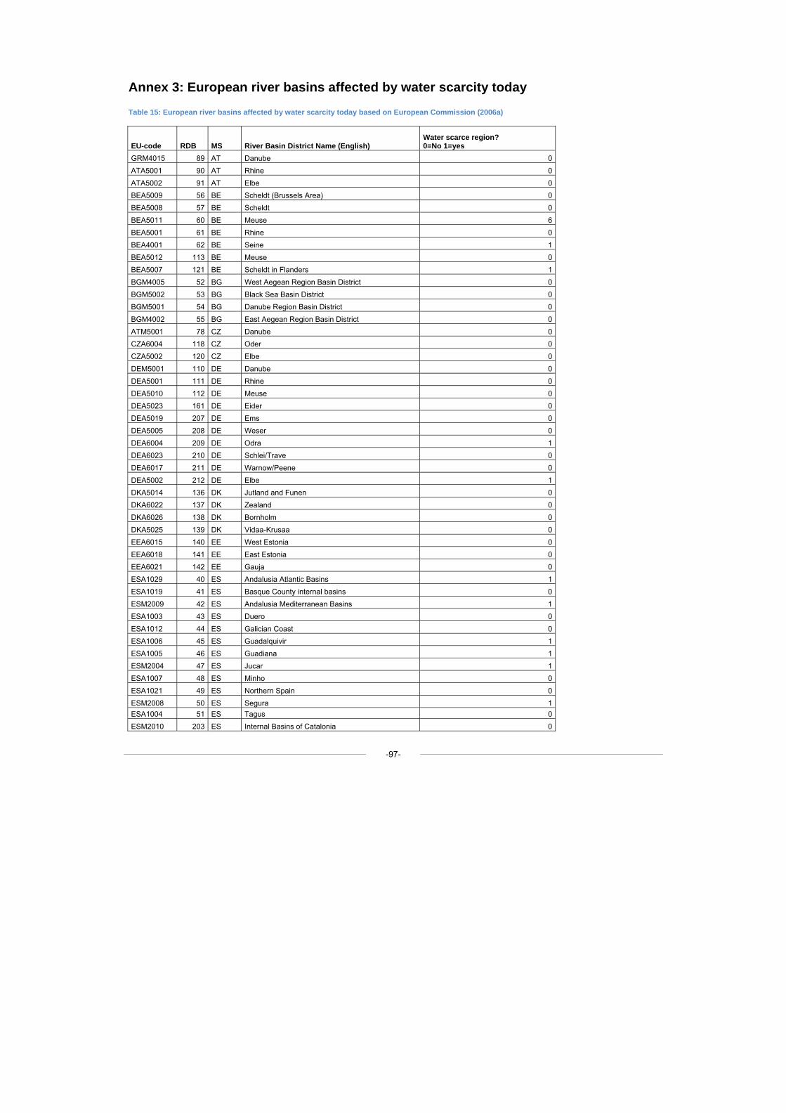
-97-

Annex 3: European river basins affected by water scarcity today

Table 15: European river basins affected by water scarcity today based on European Commission (2006a)

EU-code RDB MS River Basin District Name (English) Water scarce region? 0=No 1=yes

GRM4015 89 AT Danube 0ATA5001 90 AT Rhine 0ATA5002 91 AT Elbe 0BEA5009 56 BE Scheldt (Brussels Area) 0BEA5008 57 BE Scheldt 0BEA5011 60 BE Meuse 6BEA5001 61 BE Rhine 0BEA4001 62 BE Seine 1BEA5012 113 BE Meuse 0BEA5007 121 BE Scheldt in Flanders 1BGM4005 52 BG West Aegean Region Basin District 0BGM5002 53 BG Black Sea Basin District 0BGM5001 54 BG Danube Region Basin District 0BGM4002 55 BG East Aegean Region Basin District 0ATM5001 78 CZ Danube 0CZA6004 118 CZ Oder 0CZA5002 120 CZ Elbe 0DEM5001 110 DE Danube 0DEA5001 111 DE Rhine 0DEA5010 112 DE Meuse 0DEA5023 161 DE Eider 0DEA5019 207 DE Ems 0DEA5005 208 DE Weser 0DEA6004 209 DE Odra 1DEA6023 210 DE Schlei/Trave 0DEA6017 211 DE Warnow/Peene 0DEA5002 212 DE Elbe 1DKA5014 136 DK Jutland and Funen 0DKA6022 137 DK Zealand 0DKA6026 138 DK Bornholm 0DKA5025 139 DK Vidaa-Krusaa 0EEA6015 140 EE West Estonia 0EEA6018 141 EE East Estonia 0EEA6021 142 EE Gauja 0ESA1029 40 ES Andalusia Atlantic Basins 1ESA1019 41 ES Basque County internal basins 0ESM2009 42 ES Andalusia Mediterranean Basins 1ESA1003 43 ES Duero 0ESA1012 44 ES Galician Coast 0ESA1006 45 ES Guadalquivir 1ESA1005 46 ES Guadiana 1ESM2004 47 ES Jucar 1ESA1007 48 ES Minho 0ESA1021 49 ES Northern Spain 0ESM2008 50 ES Segura 1ESA1004 51 ES Tagus 0ESM2010 203 ES Internal Basins of Catalonia 0

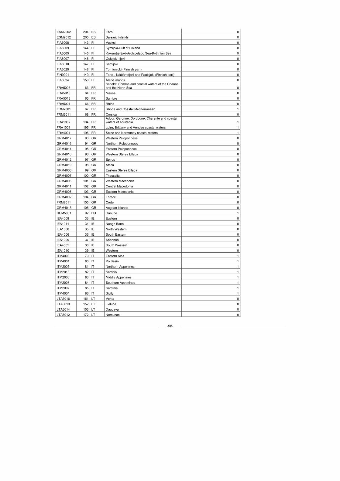
-98-

ESM2002 204 ES Ebro 0ESM2012 205 ES Balearic Islands 0FIA6008 143 FI Vuoksi 0FIA6009 144 FI Kymijoki-Gulf of Finland 0FIA6005 145 FI Kokemäenjoki-Archipelago Sea-Bothnian Sea 0FIA6007 146 FI Oulujoki-Iijoki 0FIA6010 147 FI Kemijoki 0FIA6020 148 FI Tornionjoki (Finnish part) 0FIN9001 149 FI Teno-, Näätämöjoki and Paatsjoki (Finnish part) 0FIA6024 150 FI Aland islands 0

FRA5006 63 FR Scheldt, Somme and coastal waters of the Channel and the North Sea 0

FRA5010 64 FR Meuse 0FRA5013 65 FR Sambre 0FRA5001 66 FR Rhine 0FRM2001 67 FR Rhone and Coastal Mediterranean 1FRM2011 68 FR Corsica 0

FRA1002 194 FR Adour, Garonne, Dordogne, Charente and coastal waters of aquitania 1

FRA1001 195 FR Loire, Brittany and Vendee coastal waters 1FRA4001 196 FR Seine and Normandy coastal waters 1GRM4017 93 GR Western Peloponnese 0GRM4016 94 GR Northern Peloponnese 0GRM4014 95 GR Eastern Peloponnese 0GRM4010 96 GR Western Sterea Ellada 0GRM4012 97 GR Epirus 0GRM4019 98 GR Attica 0GRM4008 99 GR Eastern Sterea Ellada 0GRM4007 100 GR Thessalia 0GRM4006 101 GR Western Macedonia 0GRM4011 102 GR Central Macedonia 0GRM4005 103 GR Eastern Macedonia 0GRM4002 104 GR Thrace 0FRM2011 105 GR Crete 0GRM4013 106 GR Aegean Islands 0HUM5001 92 HU Danube 1IEA4009 33 IE Eastern 0IEA1011 34 IE Neagh Bann 0IEA1008 35 IE North Western 0IEA4006 36 IE South Eastern 0IEA1009 37 IE Shannon 0IEA4005 38 IE South Western 0IEA1010 39 IE Western 0ITM4003 79 IT Eastern Alps 1ITM4001 80 IT Po Basin 1ITM2005 81 IT Northern Appenines 1ITM2013 82 IT Serchio 1ITM2006 83 IT Middle Appenines 1ITM2003 84 IT Southern Appenines 1ITM2007 85 IT Sardinia 1ITM4004 86 IT Sicily 1LTA6016 151 LT Venta 0LTA6019 152 LT Lielupe 0LTA6014 153 LT Daugava 0LTA6012 172 LT Nemunas 0

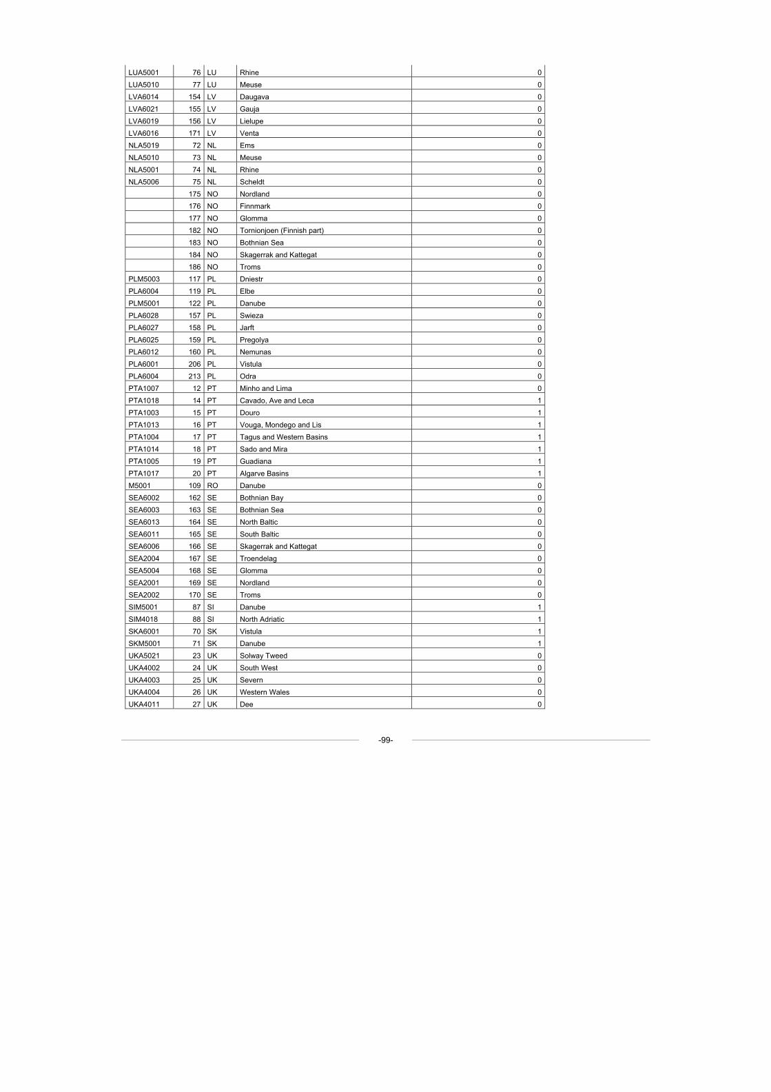
-99-

LUA5001 76 LU Rhine 0LUA5010 77 LU Meuse 0LVA6014 154 LV Daugava 0LVA6021 155 LV Gauja 0LVA6019 156 LV Lielupe 0LVA6016 171 LV Venta 0NLA5019 72 NL Ems 0NLA5010 73 NL Meuse 0NLA5001 74 NL Rhine 0NLA5006 75 NL Scheldt 0 175 NO Nordland 0 176 NO Finnmark 0 177 NO Glomma 0 182 NO Tornionjoen (Finnish part) 0 183 NO Bothnian Sea 0 184 NO Skagerrak and Kattegat 0 186 NO Troms 0PLM5003 117 PL Dniestr 0PLA6004 119 PL Elbe 0PLM5001 122 PL Danube 0PLA6028 157 PL Swieza 0PLA6027 158 PL Jarft 0PLA6025 159 PL Pregolya 0PLA6012 160 PL Nemunas 0PLA6001 206 PL Vistula 0PLA6004 213 PL Odra 0PTA1007 12 PT Minho and Lima 0PTA1018 14 PT Cavado, Ave and Leca 1PTA1003 15 PT Douro 1PTA1013 16 PT Vouga, Mondego and Lis 1PTA1004 17 PT Tagus and Western Basins 1PTA1014 18 PT Sado and Mira 1PTA1005 19 PT Guadiana 1PTA1017 20 PT Algarve Basins 1M5001 109 RO Danube 0SEA6002 162 SE Bothnian Bay 0SEA6003 163 SE Bothnian Sea 0SEA6013 164 SE North Baltic 0SEA6011 165 SE South Baltic 0SEA6006 166 SE Skagerrak and Kattegat 0SEA2004 167 SE Troendelag 0SEA5004 168 SE Glomma 0SEA2001 169 SE Nordland 0SEA2002 170 SE Troms 0SIM5001 87 SI Danube 1SIM4018 88 SI North Adriatic 1SKA6001 70 SK Vistula 1SKM5001 71 SK Danube 1UKA5021 23 UK Solway Tweed 0UKA4002 24 UK South West 0UKA4003 25 UK Severn 0UKA4004 26 UK Western Wales 0UKA4011 27 UK Dee 0

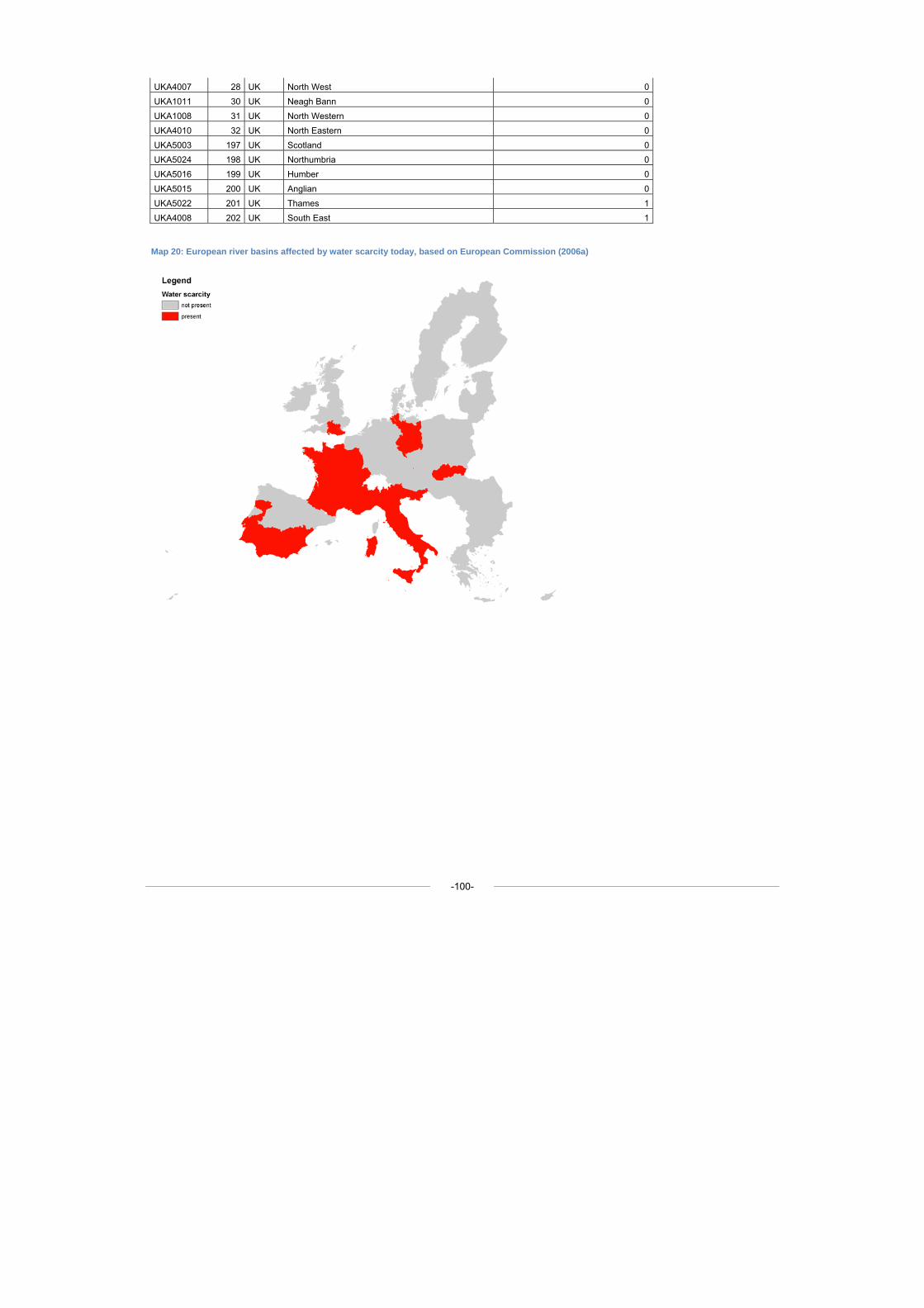
UKA4007 28 UK North West 0UKA1011 30 UK Neagh Bann 0UKA1008 31 UK North Western 0UKA4010 32 UK North Eastern 0UKA5003 197 UK Scotland 0UKA5024 198 UK Northumbria 0UKA5016 199 UK Humber 0UKA5015 200 UK Anglian 0UKA5022 201 UK Thames 1UKA4008 202 UK South East 1

Map 20: European river basins affected by water scarcity today, based on European Commission (2006a)

-100-

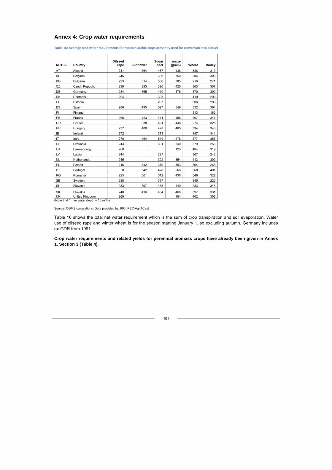
-101-

Annex 4: Crop water requirements

Table 16: Average crop water requirements for rotation arable crops presently used for conversion into biofuel

NUTS-0 Country Oilseed

rape Sunflower Sugar

beet maize

(grain) Wheat Barley

AT Austria 241 364 467 438 386 313 BE Belgium 246 389 350 384 306 BG Bulgaria 223 314 538 385 216 271 CZ Czech Republic 230 393 390 420 363 307 DE Germany 234 365 410 376 370 300 DK Denmark 294 393 419 290 EE Estonia 287 306 206 ES Spain 286 495 597 549 332 394 FI Finland 313 183 FR France 266 423 441 456 397 347 GR Greece 338 491 448 274 325 HU Hungary 237 400 428 465 394 343 IE Ireland 272 373 447 341 IT Italy 278 464 540 478 377 357 LT Lithuania 243 301 340 379 256 LU Luxembourg 260 125 404 319 LV Latvia 244 297 367 242 NL Netherlands 245 392 354 413 300 PL Poland 216 342 370 353 364 268 PT Portugal 0 542 428 566 368 401 RO Romania 225 361 512 438 348 322 SE Sweden 288 397 345 222 SI Slovenia 233 397 468 449 283 346

SK Slovakia 240 416 484 468 397 331 UK United Kingdom 269 184 402 306

(Note that 1 mm water depth = 10 m3/ha)

Source: CGMS calculations: Data provided by JRC-IPSC-Agri4Cast

Table 16 shows the total net water requirement which is the sum of crop transpiration and soil evaporation. Water use of oilseed rape and winter wheat is for the season starting January 1, so excluding autumn. Germany includes ex-GDR from 1991.

Crop water requirements and related yields for perennial biomass crops have already been given in Annex 1, Section 3 (Table 4).

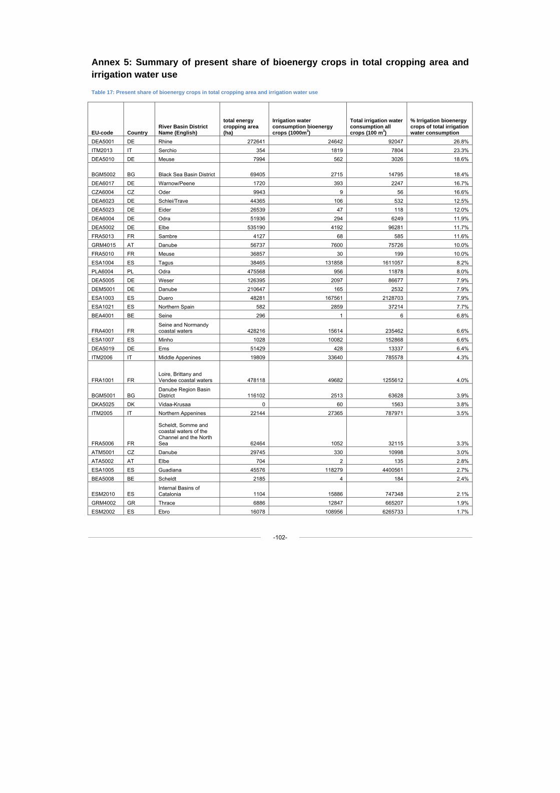
-102-

Annex 5: Summary of present share of bioenergy crops in total cropping area and irrigation water use

Table 17: Present share of bioenergy crops in total cropping area and irrigation water use

EU-code Country River Basin District Name (English)

total energy cropping area (ha)

Irrigation water consumption bioenergy crops (1000m3)

Total irrigation water consumption all crops (100 m3)

% Irrigation bioenergy crops of total irrigation water consumption

DEA5001 DE Rhine 272641 24642 92047 26.8% ITM2013 IT Serchio 354 1819 7804 23.3% DEA5010 DE Meuse 7994 562 3026 18.6%

BGM5002 BG Black Sea Basin District 69405 2715 14795 18.4%

DEA6017 DE Warnow/Peene 1720 393 2247 16.7% CZA6004 CZ Oder 9943 9 56 16.6% DEA6023 DE Schlei/Trave 44365 106 532 12.5% DEA5023 DE Eider 26539 47 118 12.0% DEA6004 DE Odra 51936 294 6249 11.9% DEA5002 DE Elbe 535190 4192 96281 11.7% FRA5013 FR Sambre 4127 68 585 11.6% GRM4015 AT Danube 56737 7600 75726 10.0% FRA5010 FR Meuse 36857 30 199 10.0% ESA1004 ES Tagus 38465 131858 1611057 8.2% PLA6004 PL Odra 475568 956 11878 8.0% DEA5005 DE Weser 126395 2097 86677 7.9% DEM5001 DE Danube 210647 165 2532 7.9% ESA1003 ES Duero 48281 167561 2128703 7.9% ESA1021 ES Northern Spain 582 2859 37214 7.7% BEA4001 BE Seine 296 1 6 6.8%

FRA4001 FR Seine and Normandy coastal waters 428216 15614 235462 6.6%

ESA1007 ES Minho 1028 10082 152868 6.6% DEA5019 DE Ems 51429 428 13337 6.4% ITM2006 IT Middle Appenines 19809 33640 785578 4.3%

FRA1001 FR Loire, Brittany and Vendee coastal waters 478118 49682 1255612 4.0%

BGM5001 BG Danube Region Basin District 116102 2513 63628 3.9%

DKA5025 DK Vidaa-Krusaa 0 60 1563 3.8% ITM2005 IT Northern Appenines 22144 27365 787971 3.5%

FRA5006 FR

Scheldt, Somme and coastal waters of the Channel and the North Sea 62464 1052 32115 3.3%

ATM5001 CZ Danube 29745 330 10998 3.0% ATA5002 AT Elbe 704 2 135 2.8% ESA1005 ES Guadiana 45576 118279 4400561 2.7% BEA5008 BE Scheldt 2185 4 184 2.4%

ESM2010 ES Internal Basins of Catalonia 1104 15886 747348 2.1%

GRM4002 GR Thrace 6886 12847 665207 1.9% ESM2002 ES Ebro 16078 108956 6265733 1.7%

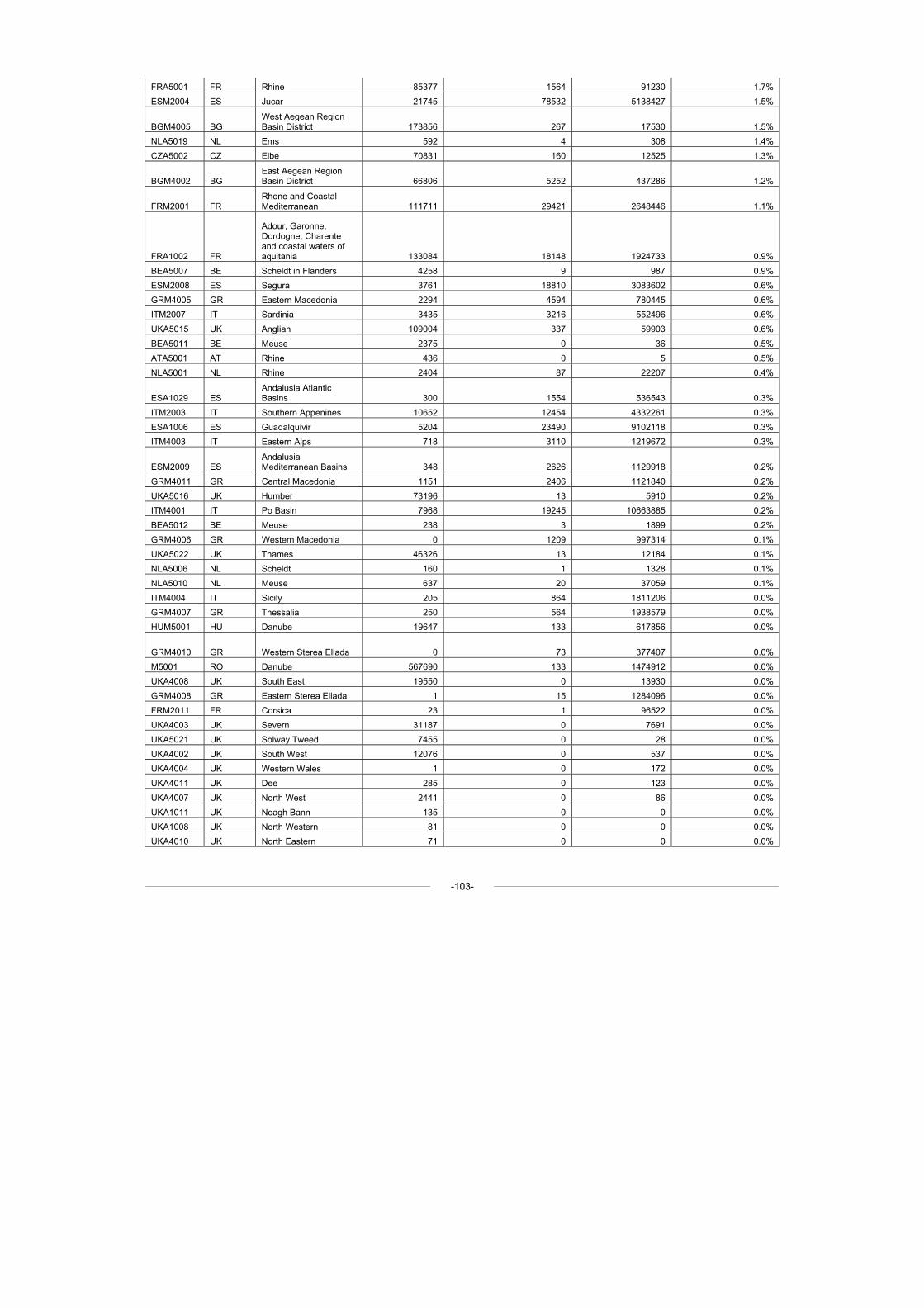
-103-

FRA5001 FR Rhine 85377 1564 91230 1.7% ESM2004 ES Jucar 21745 78532 5138427 1.5%

BGM4005 BG West Aegean Region Basin District 173856 267 17530 1.5%

NLA5019 NL Ems 592 4 308 1.4% CZA5002 CZ Elbe 70831 160 12525 1.3%

BGM4002 BG East Aegean Region Basin District 66806 5252 437286 1.2%

FRM2001 FR Rhone and Coastal Mediterranean 111711 29421 2648446 1.1%

FRA1002 FR

Adour, Garonne, Dordogne, Charente and coastal waters of aquitania 133084 18148 1924733 0.9%

BEA5007 BE Scheldt in Flanders 4258 9 987 0.9% ESM2008 ES Segura 3761 18810 3083602 0.6% GRM4005 GR Eastern Macedonia 2294 4594 780445 0.6% ITM2007 IT Sardinia 3435 3216 552496 0.6% UKA5015 UK Anglian 109004 337 59903 0.6% BEA5011 BE Meuse 2375 0 36 0.5% ATA5001 AT Rhine 436 0 5 0.5% NLA5001 NL Rhine 2404 87 22207 0.4%

ESA1029 ES Andalusia Atlantic Basins 300 1554 536543 0.3%

ITM2003 IT Southern Appenines 10652 12454 4332261 0.3% ESA1006 ES Guadalquivir 5204 23490 9102118 0.3% ITM4003 IT Eastern Alps 718 3110 1219672 0.3%

ESM2009 ES Andalusia Mediterranean Basins 348 2626 1129918 0.2%

GRM4011 GR Central Macedonia 1151 2406 1121840 0.2% UKA5016 UK Humber 73196 13 5910 0.2% ITM4001 IT Po Basin 7968 19245 10663885 0.2% BEA5012 BE Meuse 238 3 1899 0.2% GRM4006 GR Western Macedonia 0 1209 997314 0.1% UKA5022 UK Thames 46326 13 12184 0.1% NLA5006 NL Scheldt 160 1 1328 0.1% NLA5010 NL Meuse 637 20 37059 0.1% ITM4004 IT Sicily 205 864 1811206 0.0% GRM4007 GR Thessalia 250 564 1938579 0.0% HUM5001 HU Danube 19647 133 617856 0.0%

GRM4010 GR Western Sterea Ellada 0 73 377407 0.0% M5001 RO Danube 567690 133 1474912 0.0% UKA4008 UK South East 19550 0 13930 0.0% GRM4008 GR Eastern Sterea Ellada 1 15 1284096 0.0% FRM2011 FR Corsica 23 1 96522 0.0% UKA4003 UK Severn 31187 0 7691 0.0% UKA5021 UK Solway Tweed 7455 0 28 0.0% UKA4002 UK South West 12076 0 537 0.0% UKA4004 UK Western Wales 1 0 172 0.0% UKA4011 UK Dee 285 0 123 0.0% UKA4007 UK North West 2441 0 86 0.0% UKA1011 UK Neagh Bann 135 0 0 0.0% UKA1008 UK North Western 81 0 0 0.0% UKA4010 UK North Eastern 71 0 0 0.0%

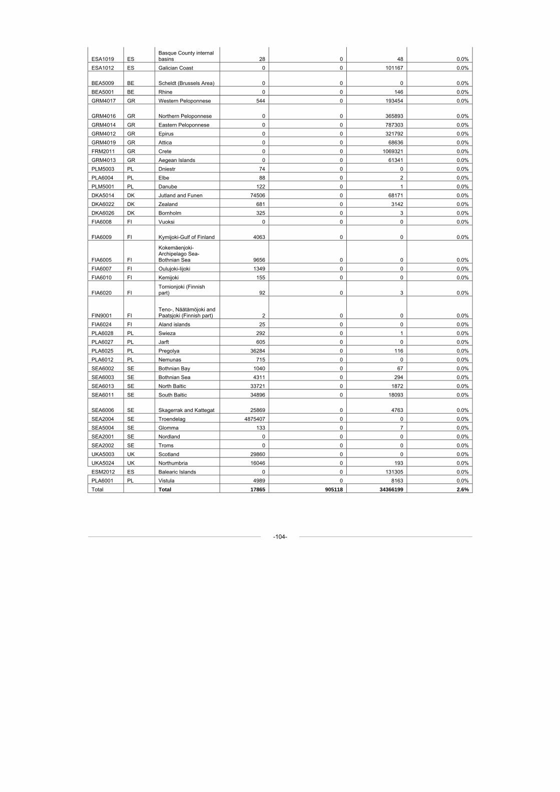
-104-

ESA1019 ES Basque County internal basins 28 0 48 0.0%

ESA1012 ES Galician Coast 0 0 101167 0.0%

BEA5009 BE Scheldt (Brussels Area) 0 0 0 0.0%

BEA5001 BE Rhine 0 0 146 0.0% GRM4017 GR Western Peloponnese 544 0 193454 0.0%

GRM4016 GR Northern Peloponnese 0 0 365893 0.0%

GRM4014 GR Eastern Peloponnese 0 0 787303 0.0% GRM4012 GR Epirus 0 0 321792 0.0% GRM4019 GR Attica 0 0 68636 0.0% FRM2011 GR Crete 0 0 1069321 0.0% GRM4013 GR Aegean Islands 0 0 61341 0.0% PLM5003 PL Dniestr 74 0 0 0.0% PLA6004 PL Elbe 88 0 2 0.0% PLM5001 PL Danube 122 0 1 0.0% DKA5014 DK Jutland and Funen 74506 0 68171 0.0% DKA6022 DK Zealand 681 0 3142 0.0% DKA6026 DK Bornholm 325 0 3 0.0% FIA6008 FI Vuoksi 0 0 0 0.0%

FIA6009 FI Kymijoki-Gulf of Finland 4063 0 0 0.0%

FIA6005 FI

Kokemäenjoki-Archipelago Sea-Bothnian Sea 9656 0 0 0.0%

FIA6007 FI Oulujoki-Iijoki 1349 0 0 0.0% FIA6010 FI Kemijoki 155 0 0 0.0%

FIA6020 FI Tornionjoki (Finnish part) 92 0 3 0.0%

FIN9001 FI Teno-, Näätämöjoki and Paatsjoki (Finnish part) 2 0 0 0.0%

FIA6024 FI Aland islands 25 0 0 0.0% PLA6028 PL Swieza 292 0 1 0.0% PLA6027 PL Jarft 605 0 0 0.0% PLA6025 PL Pregolya 36284 0 116 0.0% PLA6012 PL Nemunas 715 0 0 0.0% SEA6002 SE Bothnian Bay 1040 0 67 0.0% SEA6003 SE Bothnian Sea 4311 0 294 0.0% SEA6013 SE North Baltic 33721 0 1872 0.0% SEA6011 SE South Baltic 34896 0 18093 0.0%

SEA6006 SE Skagerrak and Kattegat 25869 0 4763 0.0%

SEA2004 SE Troendelag 4875407 0 0 0.0% SEA5004 SE Glomma 133 0 7 0.0% SEA2001 SE Nordland 0 0 0 0.0% SEA2002 SE Troms 0 0 0 0.0% UKA5003 UK Scotland 29860 0 0 0.0% UKA5024 UK Northumbria 16046 0 193 0.0% ESM2012 ES Balearic Islands 0 0 131305 0.0% PLA6001 PL Vistula 4989 0 8163 0.0% Total Total 17865 905118 34366199 2.6%

-105-

Annex 6: CAPSIM Animlib Scenario

The CAPSIM model provides results for all agricultural commodities expressed in production size, yields and land requirements by 2010, 2020 and 202518. It covers 23 MS of the European Union; Cyprus and Malta are not included due to limited data availability. The study builds on results from existing projection studies, namely the European Commission (2004) ‘Prospects for agricultural markets’ (July 2004), FAPRI, the USDA/ERS baseline model, IMPACT and FAO projections, integrating these into the CAPSIM model. In this way expert judgements from different projection studies are combined and an average projection is derived. In order to make the projections, the CAPSIM model uses a partial equilibrium modelling approach.

CAPSIM contains a broad range of social, economic, technological and policy orientated assumptions. Exogenous assumptions were split into demand and supply side factors:

Demand side:

• Population growth and household expenditure are taken from the set of key assumptions compiled by the PRIMES modelling team, given in 10-year intervals from 1990 to 2030. Because the ex post data differ from EUROSTAT population data, which provide the bulk of the CAPSIM database, the projections have been expressed in index form (relative to 2000).

• Consumption is driven by price movements and other issues (lifestyle, habits) interpreted as preference shifts over time. Price changes are partly endogenous, partly exogenous. For market clearing, either exogenous international market prices are taken, where net trade is endogenous, or exogenous net trade prices are taken, which are determined endogenously.

• Assumptions on international prices and on EU net trade are derived from the projections of international agencies. Demand and supply side interact on markets. For tradable products, international prices (border prices) are linked to EU prices using a price transmission equation based on the law of one price. Without border measures, these international prices would directly apply to EU markets. Price policy instruments are tariffs or, after tariffs are removed, administered prices with associated flexible levies or export subsidies. For non-tradable products (fodder, calves), market clearing occurs at the Member State level.

• The non-agricultural (general) price index is an important special case, which was specified in line with assumptions on the €/$ exchange rate. The exchange rate used in the baseline projection was fixed at 1.1 $/€ from 2001 onwards, in line with European Commission assumptions when the report was prepared.

Supply Side:

• The key assumptions operating on the supply side are technological changes, yield developments and price variables. Depending on the trade regime, the latter are determined through interaction with the demand side.

• CAPSIM distinguishes activity levels and yields such that crop yields, for example, are an explicit modelling input. Other changes, such as long run shifts in manure and housing systems, can only be incorporated in the form of parameter shifts of the nutrient balance description and cannot be analysed as a separate activity.

• Regarding structural change of farm size distribution, part time farming and labour force changes, explicit analysis goes beyond the scope of CAPSIM. However, structural change may be considered as a special

18 Extrapolated to 2030 for the purpose of this study; see Section 3.2.1.

-106-

type of technological change, when viewed from an aggregate perspective. Considerable efforts have been made to capture the bottom line of these shifts in behavioural functions on the supply and demand side with a sophisticated set of trend projections. These trend projections incorporate a significant number of technological constraints (nutrient balances, land balance) as well as identities (production = area * yield) to compensate for detailed modelling of the individual contributions to overall technological change, such as genetic improvements, capital accumulation, input quality and structural change.

• Policy strongly influences incentives on the supply side. The gross revenues from operations are the result of both market revenues and different types of CAP payments.

• Obligatory set aside is specified according to the July 2004 DG Agriculture projections. Non-food production is treated in the same manner.

The behavioural functions in the CAPSIM model – which include functions for activity levels, input demand, consumer demand and processing – may shift over time. They usually reflect linear or nonlinear impacts of technological or structural change.

In the Animlib scenario, the quota regime for milk ends in 2025. This is preceded by a gradual drop in the administrative prices for butter and skimmed milk powder as well as tariffs for dairy products, starting after 2011. Similarly, market interventions for beef are eliminated, and tariffs for the different meats and eggs are removed. Consequently, EU market prices are assumed to be identical to border (world market) prices in the year 2025. The reduction in milk prices also decreases quota rents. Once those reach zero, dairy cow herds (-10%) adjust until marginal production costs are equal to the reduced milk price (-33%). Additionally, the lower price of beef (-30%) compared to the reference run will reduce beef production (-4%). At the same time, market prices for pork (-13%) and poultry (-28%) will line up with world markets, and herds adjust (-5% for pigs and -11% for poultry). The reduced herd sizes also lower the demand for fodder and allow a reduction of the fodder area (-2%), which in turn leads to an expansion of other crops (cereals: +1%).

The remaining coupled payments are for protein crops and for paddy rice (compensation for strong price cut). The only relevant intervention price is for sugar, which has been decreased according to the 2004 Commission proposal (down from 632 € to 421 €)19. Intervention prices for cereals remain in place, but they become irrelevant as world prices are assumed to increase (in nominal terms) and become equivalent or even higher than EU prices from 2020 onwards.

19 This does not incorporate the sugar reform agreement from December 2005. Overall, however, the assumptions used in CAPSIM do not diverge significantly from the present agreement.

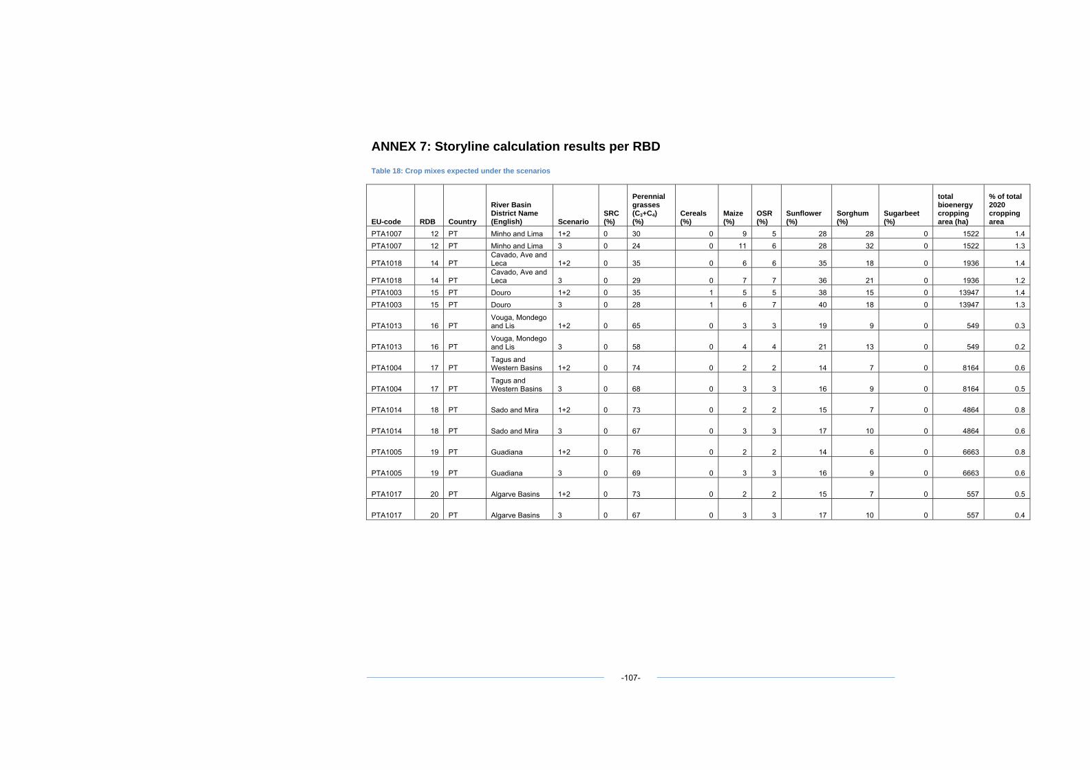
ANNEX 7: Storyline calculation results per RBD

Table 18: Crop mixes expected under the scenarios

EU-code RDB Country

River Basin District Name (English) Scenario

SRC (%)

Perennial grasses (C3+C4) (%)

Cereals (%)

Maize (%)

OSR (%)

Sunflower (%)

Sorghum (%)

Sugarbeet (%)

total bioenergy cropping area (ha)

% of total 2020 cropping area

PTA1007 12 PT Minho and Lima 1+2 0 30 0 9 5 28 28 0 1522 1.4 PTA1007 12 PT Minho and Lima 3 0 24 0 11 6 28 32 0 1522 1.3

PTA1018 14 PT Cavado, Ave and Leca 1+2 0 35 0 6 6 35 18 0 1936 1.4

PTA1018 14 PT Cavado, Ave and Leca 3 0 29 0 7 7 36 21 0 1936 1.2

PTA1003 15 PT Douro 1+2 0 35 1 5 5 38 15 0 13947 1.4 PTA1003 15 PT Douro 3 0 28 1 6 7 40 18 0 13947 1.3

PTA1013 16 PT Vouga, Mondego and Lis 1+2 0 65 0 3 3 19 9 0 549 0.3

PTA1013 16 PT Vouga, Mondego and Lis 3 0 58 0 4 4 21 13 0 549 0.2

PTA1004 17 PT Tagus and Western Basins 1+2 0 74 0 2 2 14 7 0 8164 0.6

PTA1004 17 PT Tagus and Western Basins 3 0 68 0 3 3 16 9 0 8164 0.5

PTA1014 18 PT Sado and Mira 1+2 0 73 0 2 2 15 7 0 4864 0.8

PTA1014 18 PT Sado and Mira 3 0 67 0 3 3 17 10 0 4864 0.6

PTA1005 19 PT Guadiana 1+2 0 76 0 2 2 14 6 0 6663 0.8

PTA1005 19 PT Guadiana 3 0 69 0 3 3 16 9 0 6663 0.6

PTA1017 20 PT Algarve Basins 1+2 0 73 0 2 2 15 7 0 557 0.5

PTA1017 20 PT Algarve Basins 3 0 67 0 3 3 17 10 0 557 0.4

-107-

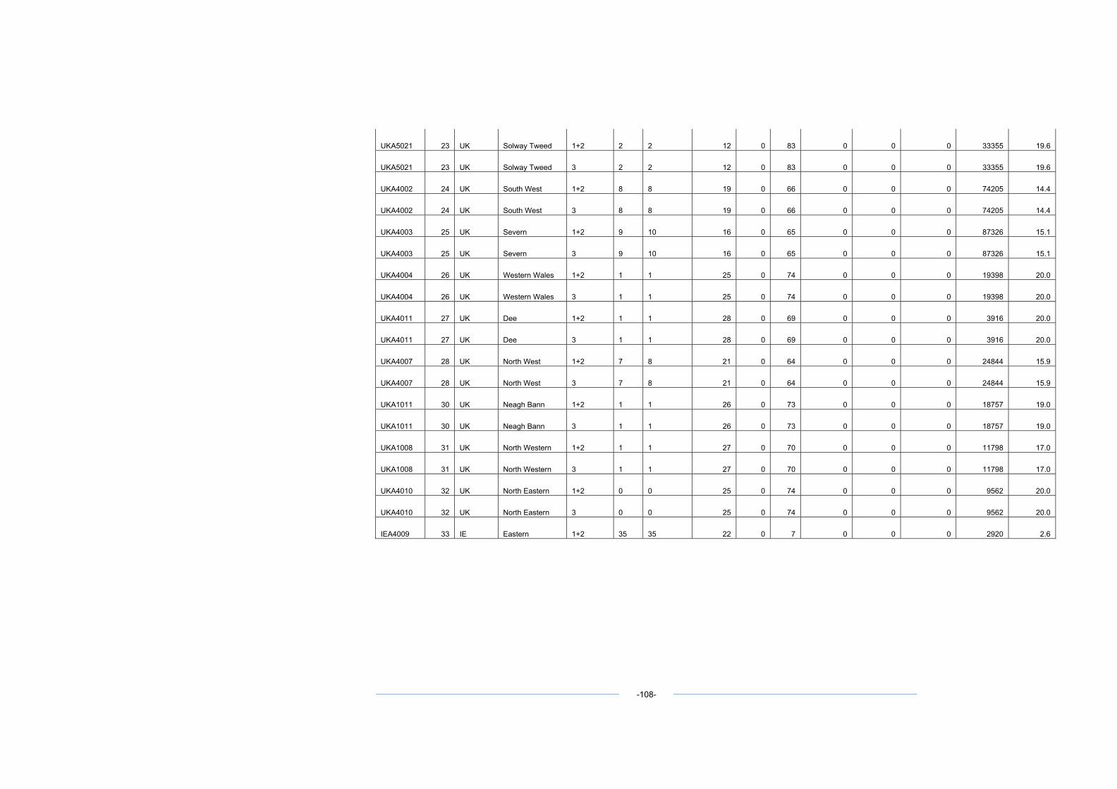
UKA5021 23 UK Solway Tweed 1+2 2 2 12 0 83 0 0 0 33355 19.6

UKA5021 23 UK Solway Tweed 3 2 2 12 0 83 0 0 0 33355 19.6

UKA4002 24 UK South West 1+2 8 8 19 0 66 0 0 0 74205 14.4

UKA4002 24 UK South West 3 8 8 19 0 66 0 0 0 74205 14.4

UKA4003 25 UK Severn 1+2 9 10 16 0 65 0 0 0 87326 15.1

UKA4003 25 UK Severn 3 9 10 16 0 65 0 0 0 87326 15.1

UKA4004 26 UK Western Wales 1+2 1 1 25 0 74 0 0 0 19398 20.0

UKA4004 26 UK Western Wales 3 1 1 25 0 74 0 0 0 19398 20.0

UKA4011 27 UK Dee 1+2 1 1 28 0 69 0 0 0 3916 20.0

UKA4011 27 UK Dee 3 1 1 28 0 69 0 0 0 3916 20.0

UKA4007 28 UK North West 1+2 7 8 21 0 64 0 0 0 24844 15.9

UKA4007 28 UK North West 3 7 8 21 0 64 0 0 0 24844 15.9

UKA1011 30 UK Neagh Bann 1+2 1 1 26 0 73 0 0 0 18757 19.0

UKA1011 30 UK Neagh Bann 3 1 1 26 0 73 0 0 0 18757 19.0

UKA1008 31 UK North Western 1+2 1 1 27 0 70 0 0 0 11798 17.0

UKA1008 31 UK North Western 3 1 1 27 0 70 0 0 0 11798 17.0

UKA4010 32 UK North Eastern 1+2 0 0 25 0 74 0 0 0 9562 20.0

UKA4010 32 UK North Eastern 3 0 0 25 0 74 0 0 0 9562 20.0

IEA4009 33 IE Eastern 1+2 35 35 22 0 7 0 0 0 2920 2.6

-108-

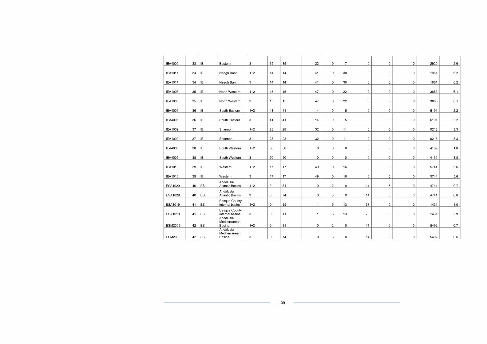
IEA4009 33 IE Eastern 3 35 35 22 0 7 0 0 0 2920 2.6

IEA1011 34 IE Neagh Bann 1+2 14 14 41 0 30 0 0 0 1961 6.2

IEA1011 34 IE Neagh Bann 3 14 14 41 0 30 0 0 0 1961 6.2

IEA1008 35 IE North Western 1+2 15 15 47 0 22 0 0 0 3883 6.1

IEA1008 35 IE North Western 3 15 15 47 0 22 0 0 0 3883 6.1

IEA4006 36 IE South Eastern 1+2 41 41 14 0 5 0 0 0 6191 2.2

IEA4006 36 IE South Eastern 3 41 41 14 0 5 0 0 0 6191 2.2

IEA1009 37 IE Shannon 1+2 28 28 32 0 11 0 0 0 9218 3.3

IEA1009 37 IE Shannon 3 28 28 32 0 11 0 0 0 9218 3.3

IEA4005 38 IE South Western 1+2 50 50 0 0 0 0 0 0 4169 1.8

IEA4005 38 IE South Western 3 50 50 0 0 0 0 0 0 4169 1.8

IEA1010 39 IE Western 1+2 17 17 49 0 16 0 0 0 5744 5.6

IEA1010 39 IE Western 3 17 17 49 0 16 0 0 0 5744 5.6

ESA1029 40 ES Andalusia Atlantic Basins 1+2 0 81 0 2 0 11 6 0 4741 0.7

ESA1029 40 ES Andalusia Atlantic Basins 3 0 74 0 3 0 14 8 0 4741 0.6

ESA1019 41 ES Basque County internal basins 1+2 0 15 1 5 13 67 0 0 1431 3.0

ESA1019 41 ES Basque County internal basins 3 0 11 1 5 13 70 0 0 1431 2.9

ESM2009 42 ES

Andalusia Mediterranean Basins 1+2 0 81 0 2 0 11 6 0 5492 0.7

ESM2009 42 ES

Andalusia Mediterranean Basins 3 0 74 0 3 0 14 8 0 5492 0.6

-109-

ESA1003 43 ES Duero 1+2 0 33 2 3 5 47 10 0 214449 2.3

ESA1003 43 ES Duero 3 0 25 2 4 5 52 11 0 214449 2.1

ESA1012 44 ES Galician Coast 1+2 0 12 0 22 0 0 66 0 4908 1.7

ESA1012 44 ES Galician Coast 3 0 8 0 23 0 0 69 0 4908 1.6

ESA1006 45 ES Guadalquivir 1+2 0 71 2 2 0 19 7 0 41682 0.9

ESA1006 45 ES Guadalquivir 3 0 62 2 3 0 24 9 0 41682 0.7

ESA1005 46 ES Guadiana 1+2 0 42 7 3 0 40 8 0 154710 2.2

ESA1005 46 ES Guadiana 3 0 33 7 3 0 47 9 0 154710 1.9

ESM2004 47 ES Jucar 1+2 0 37 6 3 0 44 10 0 88819 2.2

ESM2004 47 ES Jucar 3 0 29 6 4 1 50 11 0 88819 2.0

ESA1007 48 ES Minho 1+2 0 22 1 14 2 21 40 0 10237 1.9

ESA1007 48 ES Minho 3 0 16 1 15 2 23 43 0 10237 1.8

ESA1021 49 ES Northern Spain 1+2 0 17 1 22 6 40 14 0 9106 3.0

ESA1021 49 ES Northern Spain 3 0 12 1 23 7 43 14 0 9106 2.8

ESM2008 50 ES Segura 1+2 0 43 3 4 0 39 12 0 33093 1.8

ESM2008 50 ES Segura 3 0 34 3 5 0 45 14 0 33093 1.6

ESA1004 51 ES Tagus 1+2 0 42 6 3 0 40 9 0 138879 2.2

ESA1004 51 ES Tagus 3 0 33 7 3 0 46 10 0 138879 2.0

BGM4005 52 BG

West Aegean Region Basin District 1+2 6 19 31 0 6 38 0 0 33625 5.6

-110-

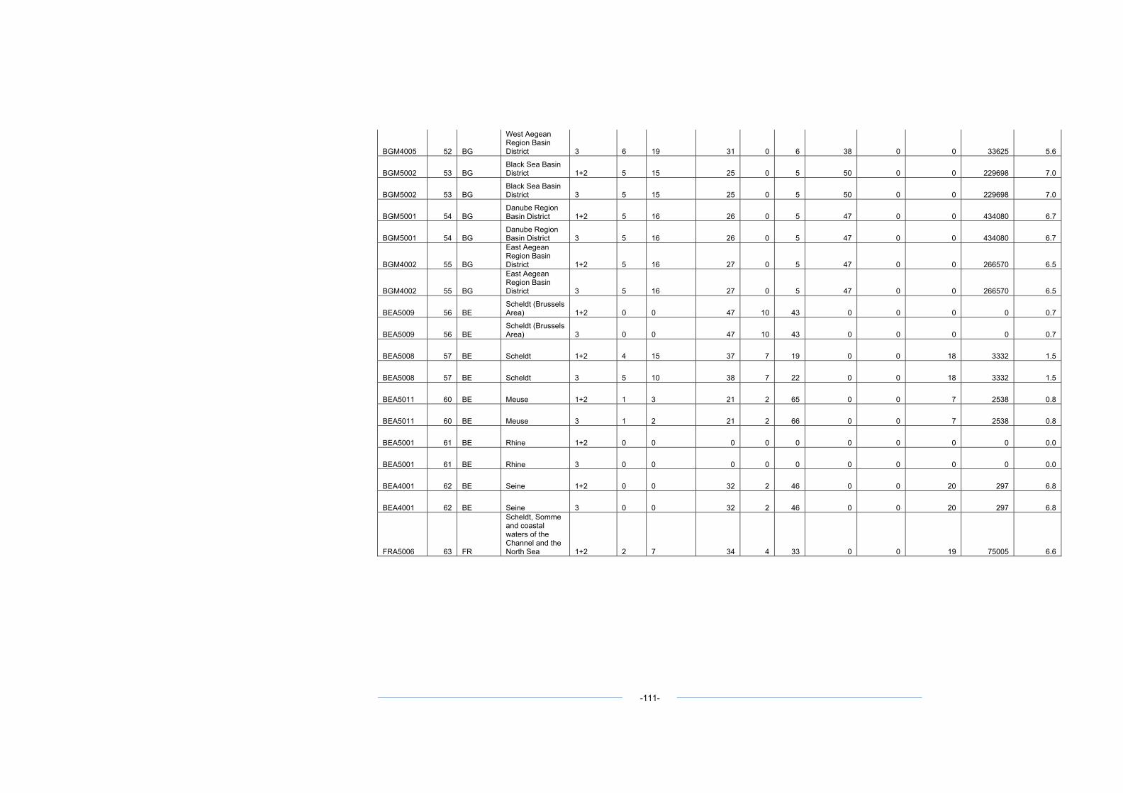
BGM4005 52 BG

West Aegean Region Basin District 3 6 19 31 0 6 38 0 0 33625 5.6

BGM5002 53 BG Black Sea Basin District 1+2 5 15 25 0 5 50 0 0 229698 7.0

BGM5002 53 BG Black Sea Basin District 3 5 15 25 0 5 50 0 0 229698 7.0

BGM5001 54 BG Danube Region Basin District 1+2 5 16 26 0 5 47 0 0 434080 6.7

BGM5001 54 BG Danube Region Basin District 3 5 16 26 0 5 47 0 0 434080 6.7

BGM4002 55 BG

East Aegean Region Basin District 1+2 5 16 27 0 5 47 0 0 266570 6.5

BGM4002 55 BG

East Aegean Region Basin District 3 5 16 27 0 5 47 0 0 266570 6.5

BEA5009 56 BE Scheldt (Brussels Area) 1+2 0 0 47 10 43 0 0 0 0 0.7

BEA5009 56 BE Scheldt (Brussels Area) 3 0 0 47 10 43 0 0 0 0 0.7

BEA5008 57 BE Scheldt 1+2 4 15 37 7 19 0 0 18 3332 1.5

BEA5008 57 BE Scheldt 3 5 10 38 7 22 0 0 18 3332 1.5

BEA5011 60 BE Meuse 1+2 1 3 21 2 65 0 0 7 2538 0.8

BEA5011 60 BE Meuse 3 1 2 21 2 66 0 0 7 2538 0.8

BEA5001 61 BE Rhine 1+2 0 0 0 0 0 0 0 0 0 0.0

BEA5001 61 BE Rhine 3 0 0 0 0 0 0 0 0 0 0.0

BEA4001 62 BE Seine 1+2 0 0 32 2 46 0 0 20 297 6.8

BEA4001 62 BE Seine 3 0 0 32 2 46 0 0 20 297 6.8

FRA5006 63 FR

Scheldt, Somme and coastal waters of the Channel and the North Sea 1+2 2 7 34 4 33 0 0 19 75005 6.6

-111-

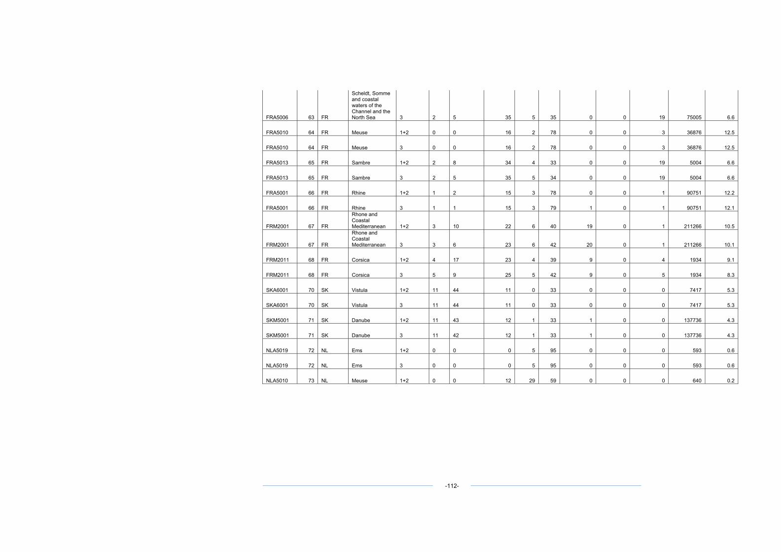
FRA5006 63 FR

Scheldt, Somme and coastal waters of the Channel and the North Sea 3 2 5 35 5 35 0 0 19 75005 6.6

FRA5010 64 FR Meuse 1+2 0 0 16 2 78 0 0 3 36876 12.5

FRA5010 64 FR Meuse 3 0 0 16 2 78 0 0 3 36876 12.5

FRA5013 65 FR Sambre 1+2 2 8 34 4 33 0 0 19 5004 6.6

FRA5013 65 FR Sambre 3 2 5 35 5 34 0 0 19 5004 6.6

FRA5001 66 FR Rhine 1+2 1 2 15 3 78 0 0 1 90751 12.2

FRA5001 66 FR Rhine 3 1 1 15 3 79 1 0 1 90751 12.1

FRM2001 67 FR

Rhone and Coastal Mediterranean 1+2 3 10 22 6 40 19 0 1 211266 10.5

FRM2001 67 FR

Rhone and Coastal Mediterranean 3 3 6 23 6 42 20 0 1 211266 10.1

FRM2011 68 FR Corsica 1+2 4 17 23 4 39 9 0 4 1934 9.1

FRM2011 68 FR Corsica 3 5 9 25 5 42 9 0 5 1934 8.3

SKA6001 70 SK Vistula 1+2 11 44 11 0 33 0 0 0 7417 5.3

SKA6001 70 SK Vistula 3 11 44 11 0 33 0 0 0 7417 5.3

SKM5001 71 SK Danube 1+2 11 43 12 1 33 1 0 0 137736 4.3

SKM5001 71 SK Danube 3 11 42 12 1 33 1 0 0 137736 4.3

NLA5019 72 NL Ems 1+2 0 0 0 5 95 0 0 0 593 0.6

NLA5019 72 NL Ems 3 0 0 0 5 95 0 0 0 593 0.6

NLA5010 73 NL Meuse 1+2 0 0 12 29 59 0 0 0 640 0.2

-112-

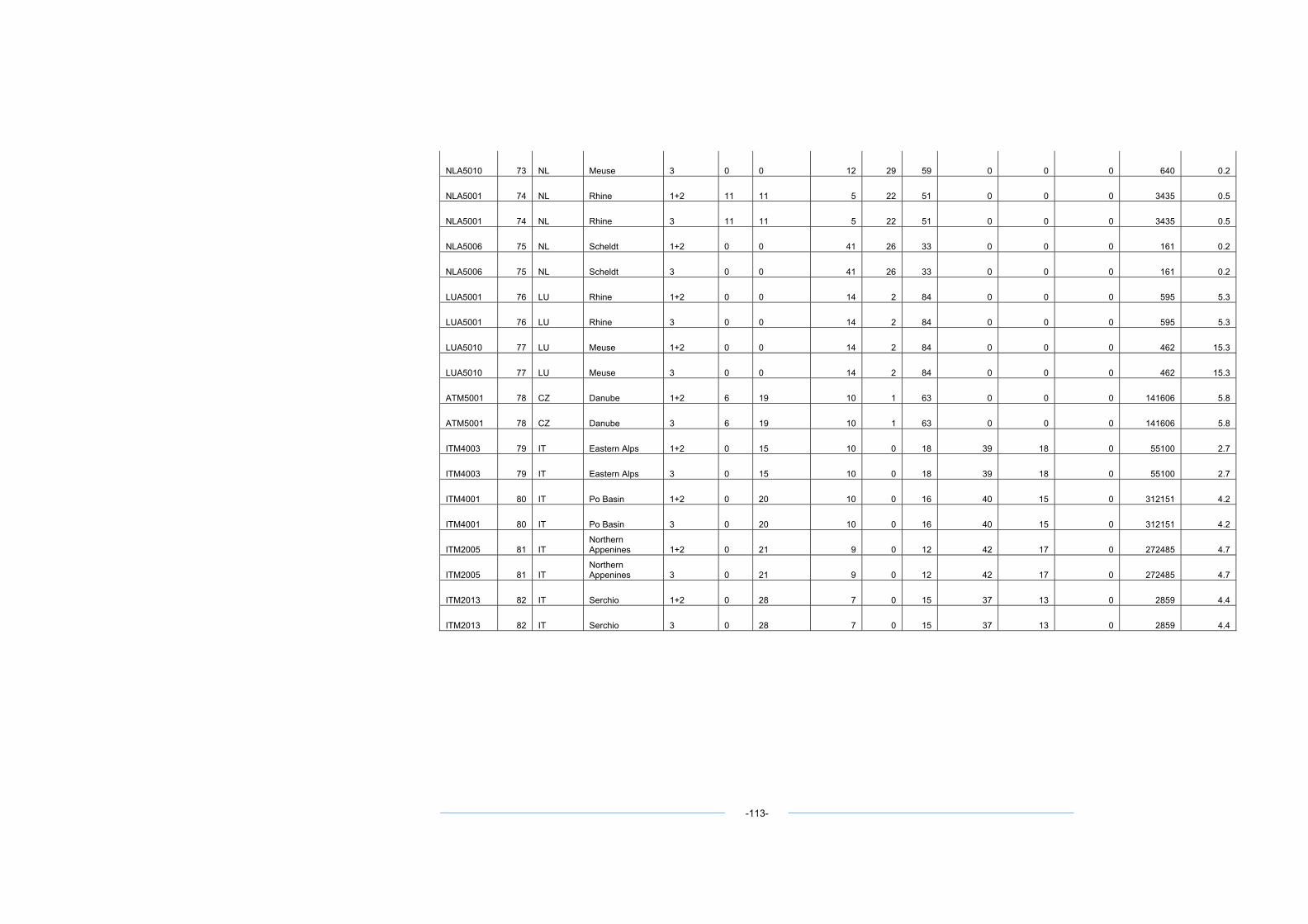
NLA5010 73 NL Meuse 3 0 0 12 29 59 0 0 0 640 0.2

NLA5001 74 NL Rhine 1+2 11 11 5 22 51 0 0 0 3435 0.5

NLA5001 74 NL Rhine 3 11 11 5 22 51 0 0 0 3435 0.5

NLA5006 75 NL Scheldt 1+2 0 0 41 26 33 0 0 0 161 0.2

NLA5006 75 NL Scheldt 3 0 0 41 26 33 0 0 0 161 0.2

LUA5001 76 LU Rhine 1+2 0 0 14 2 84 0 0 0 595 5.3

LUA5001 76 LU Rhine 3 0 0 14 2 84 0 0 0 595 5.3

LUA5010 77 LU Meuse 1+2 0 0 14 2 84 0 0 0 462 15.3

LUA5010 77 LU Meuse 3 0 0 14 2 84 0 0 0 462 15.3

ATM5001 78 CZ Danube 1+2 6 19 10 1 63 0 0 0 141606 5.8

ATM5001 78 CZ Danube 3 6 19 10 1 63 0 0 0 141606 5.8

ITM4003 79 IT Eastern Alps 1+2 0 15 10 0 18 39 18 0 55100 2.7

ITM4003 79 IT Eastern Alps 3 0 15 10 0 18 39 18 0 55100 2.7

ITM4001 80 IT Po Basin 1+2 0 20 10 0 16 40 15 0 312151 4.2

ITM4001 80 IT Po Basin 3 0 20 10 0 16 40 15 0 312151 4.2

ITM2005 81 IT Northern Appenines 1+2 0 21 9 0 12 42 17 0 272485 4.7

ITM2005 81 IT Northern Appenines 3 0 21 9 0 12 42 17 0 272485 4.7

ITM2013 82 IT Serchio 1+2 0 28 7 0 15 37 13 0 2859 4.4

ITM2013 82 IT Serchio 3 0 28 7 0 15 37 13 0 2859 4.4

-113-

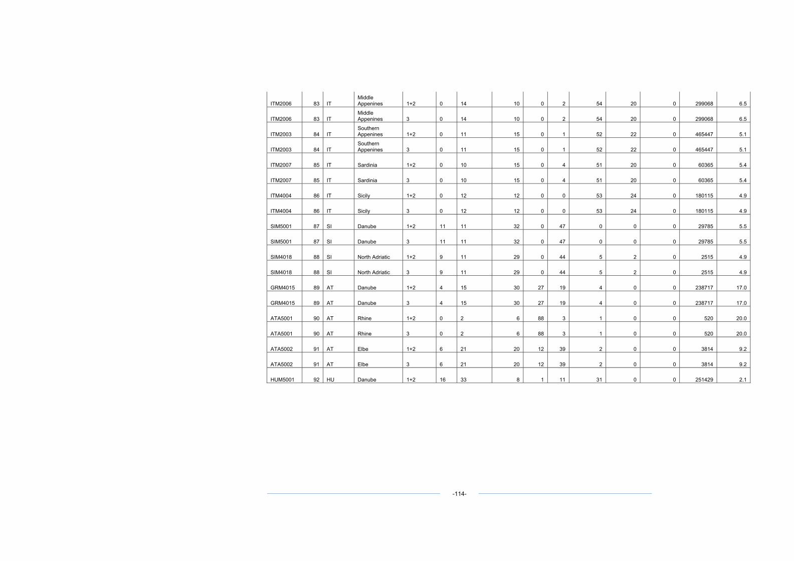
ITM2006 83 IT Middle Appenines 1+2 0 14 10 0 2 54 20 0 299068 6.5

ITM2006 83 IT Middle Appenines 3 0 14 10 0 2 54 20 0 299068 6.5

ITM2003 84 IT Southern Appenines 1+2 0 11 15 0 1 52 22 0 465447 5.1

ITM2003 84 IT Southern Appenines 3 0 11 15 0 1 52 22 0 465447 5.1

ITM2007 85 IT Sardinia 1+2 0 10 15 0 4 51 20 0 60365 5.4

ITM2007 85 IT Sardinia 3 0 10 15 0 4 51 20 0 60365 5.4

ITM4004 86 IT Sicily 1+2 0 12 12 0 0 53 24 0 180115 4.9

ITM4004 86 IT Sicily 3 0 12 12 0 0 53 24 0 180115 4.9

SIM5001 87 SI Danube 1+2 11 11 32 0 47 0 0 0 29785 5.5

SIM5001 87 SI Danube 3 11 11 32 0 47 0 0 0 29785 5.5

SIM4018 88 SI North Adriatic 1+2 9 11 29 0 44 5 2 0 2515 4.9

SIM4018 88 SI North Adriatic 3 9 11 29 0 44 5 2 0 2515 4.9

GRM4015 89 AT Danube 1+2 4 15 30 27 19 4 0 0 238717 17.0

GRM4015 89 AT Danube 3 4 15 30 27 19 4 0 0 238717 17.0

ATA5001 90 AT Rhine 1+2 0 2 6 88 3 1 0 0 520 20.0

ATA5001 90 AT Rhine 3 0 2 6 88 3 1 0 0 520 20.0

ATA5002 91 AT Elbe 1+2 6 21 20 12 39 2 0 0 3814 9.2

ATA5002 91 AT Elbe 3 6 21 20 12 39 2 0 0 3814 9.2

HUM5001 92 HU Danube 1+2 16 33 8 1 11 31 0 0 251429 2.1

-114-

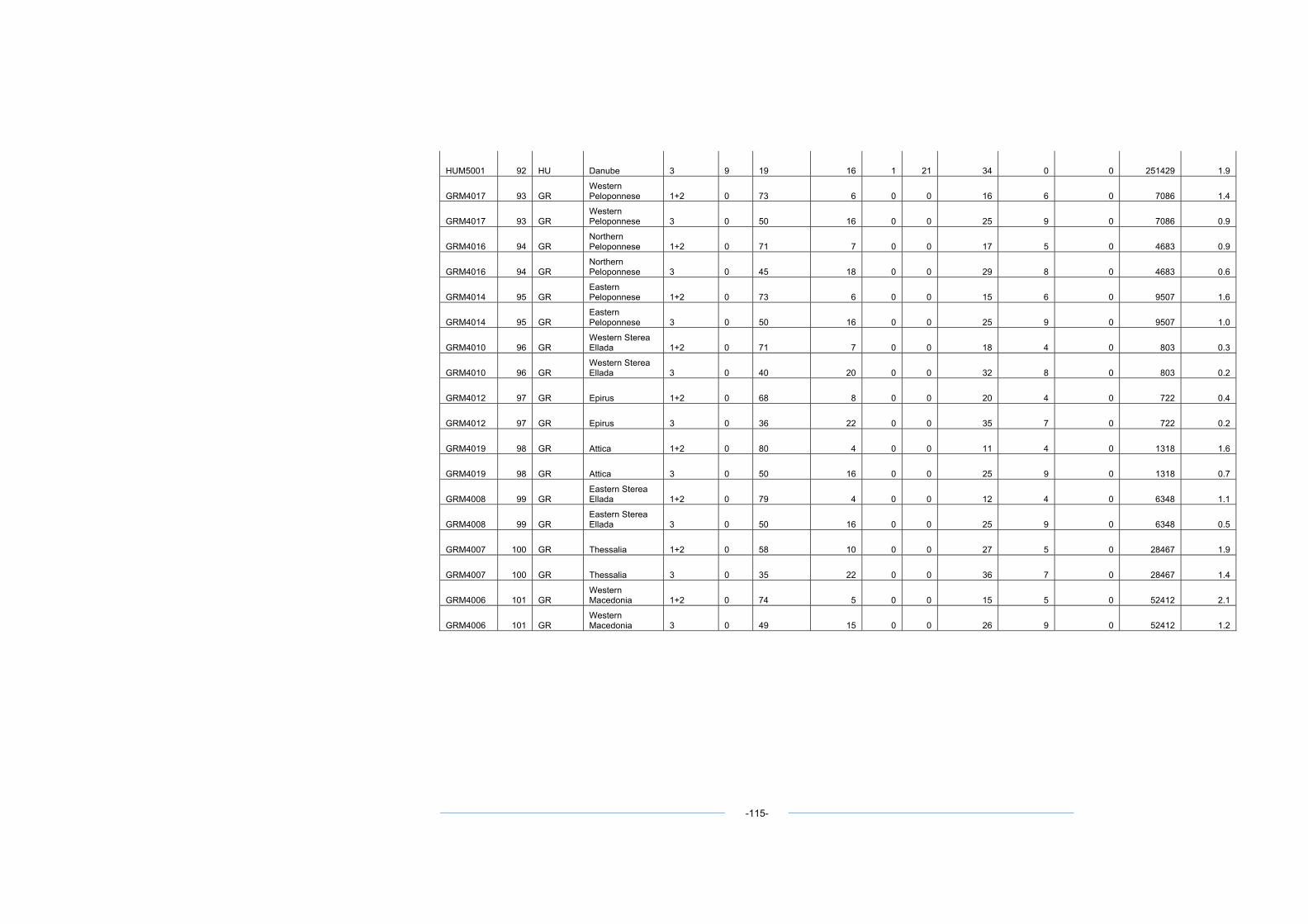
HUM5001 92 HU Danube 3 9 19 16 1 21 34 0 0 251429 1.9

GRM4017 93 GR Western Peloponnese 1+2 0 73 6 0 0 16 6 0 7086 1.4

GRM4017 93 GR Western Peloponnese 3 0 50 16 0 0 25 9 0 7086 0.9

GRM4016 94 GR Northern Peloponnese 1+2 0 71 7 0 0 17 5 0 4683 0.9

GRM4016 94 GR Northern Peloponnese 3 0 45 18 0 0 29 8 0 4683 0.6

GRM4014 95 GR Eastern Peloponnese 1+2 0 73 6 0 0 15 6 0 9507 1.6

GRM4014 95 GR Eastern Peloponnese 3 0 50 16 0 0 25 9 0 9507 1.0

GRM4010 96 GR Western Sterea Ellada 1+2 0 71 7 0 0 18 4 0 803 0.3

GRM4010 96 GR Western Sterea Ellada 3 0 40 20 0 0 32 8 0 803 0.2

GRM4012 97 GR Epirus 1+2 0 68 8 0 0 20 4 0 722 0.4

GRM4012 97 GR Epirus 3 0 36 22 0 0 35 7 0 722 0.2

GRM4019 98 GR Attica 1+2 0 80 4 0 0 11 4 0 1318 1.6

GRM4019 98 GR Attica 3 0 50 16 0 0 25 9 0 1318 0.7

GRM4008 99 GR Eastern Sterea Ellada 1+2 0 79 4 0 0 12 4 0 6348 1.1

GRM4008 99 GR Eastern Sterea Ellada 3 0 50 16 0 0 25 9 0 6348 0.5

GRM4007 100 GR Thessalia 1+2 0 58 10 0 0 27 5 0 28467 1.9

GRM4007 100 GR Thessalia 3 0 35 22 0 0 36 7 0 28467 1.4

GRM4006 101 GR Western Macedonia 1+2 0 74 5 0 0 15 5 0 52412 2.1

GRM4006 101 GR Western Macedonia 3 0 49 15 0 0 26 9 0 52412 1.2

-115-

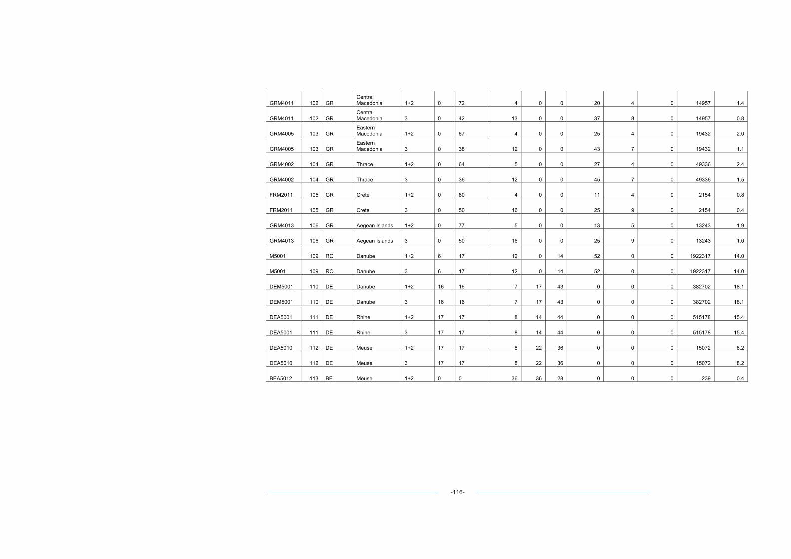
GRM4011 102 GR Central Macedonia 1+2 0 72 4 0 0 20 4 0 14957 1.4

GRM4011 102 GR Central Macedonia 3 0 42 13 0 0 37 8 0 14957 0.8

GRM4005 103 GR Eastern Macedonia 1+2 0 67 4 0 0 25 4 0 19432 2.0

GRM4005 103 GR Eastern Macedonia 3 0 38 12 0 0 43 7 0 19432 1.1

GRM4002 104 GR Thrace 1+2 0 64 5 0 0 27 4 0 49336 2.4

GRM4002 104 GR Thrace 3 0 36 12 0 0 45 7 0 49336 1.5

FRM2011 105 GR Crete 1+2 0 80 4 0 0 11 4 0 2154 0.8

FRM2011 105 GR Crete 3 0 50 16 0 0 25 9 0 2154 0.4

GRM4013 106 GR Aegean Islands 1+2 0 77 5 0 0 13 5 0 13243 1.9

GRM4013 106 GR Aegean Islands 3 0 50 16 0 0 25 9 0 13243 1.0

M5001 109 RO Danube 1+2 6 17 12 0 14 52 0 0 1922317 14.0

M5001 109 RO Danube 3 6 17 12 0 14 52 0 0 1922317 14.0

DEM5001 110 DE Danube 1+2 16 16 7 17 43 0 0 0 382702 18.1

DEM5001 110 DE Danube 3 16 16 7 17 43 0 0 0 382702 18.1

DEA5001 111 DE Rhine 1+2 17 17 8 14 44 0 0 0 515178 15.4

DEA5001 111 DE Rhine 3 17 17 8 14 44 0 0 0 515178 15.4

DEA5010 112 DE Meuse 1+2 17 17 8 22 36 0 0 0 15072 8.2

DEA5010 112 DE Meuse 3 17 17 8 22 36 0 0 0 15072 8.2

BEA5012 113 BE Meuse 1+2 0 0 36 36 28 0 0 0 239 0.4

-116-

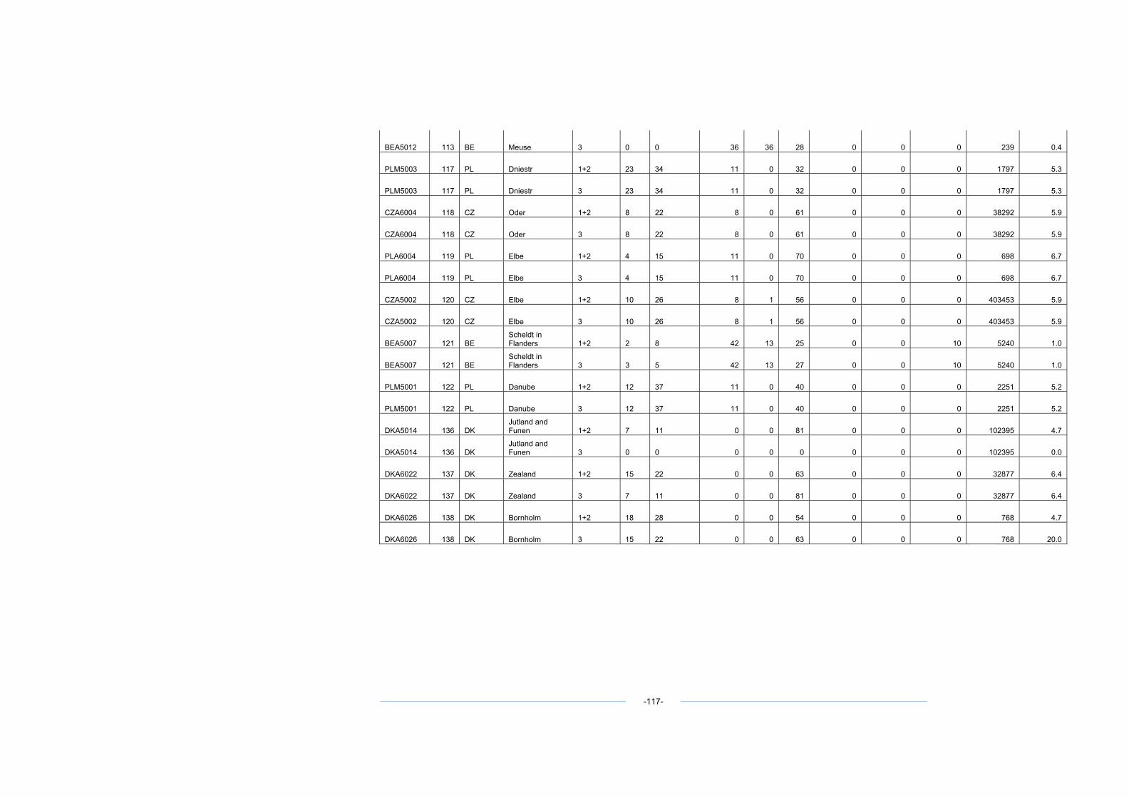
BEA5012 113 BE Meuse 3 0 0 36 36 28 0 0 0 239 0.4

PLM5003 117 PL Dniestr 1+2 23 34 11 0 32 0 0 0 1797 5.3

PLM5003 117 PL Dniestr 3 23 34 11 0 32 0 0 0 1797 5.3

CZA6004 118 CZ Oder 1+2 8 22 8 0 61 0 0 0 38292 5.9

CZA6004 118 CZ Oder 3 8 22 8 0 61 0 0 0 38292 5.9

PLA6004 119 PL Elbe 1+2 4 15 11 0 70 0 0 0 698 6.7

PLA6004 119 PL Elbe 3 4 15 11 0 70 0 0 0 698 6.7

CZA5002 120 CZ Elbe 1+2 10 26 8 1 56 0 0 0 403453 5.9

CZA5002 120 CZ Elbe 3 10 26 8 1 56 0 0 0 403453 5.9

BEA5007 121 BE Scheldt in Flanders 1+2 2 8 42 13 25 0 0 10 5240 1.0

BEA5007 121 BE Scheldt in Flanders 3 3 5 42 13 27 0 0 10 5240 1.0

PLM5001 122 PL Danube 1+2 12 37 11 0 40 0 0 0 2251 5.2

PLM5001 122 PL Danube 3 12 37 11 0 40 0 0 0 2251 5.2

DKA5014 136 DK Jutland and Funen 1+2 7 11 0 0 81 0 0 0 102395 4.7

DKA5014 136 DK Jutland and Funen 3 0 0 0 0 0 0 0 0 102395 0.0

DKA6022 137 DK Zealand 1+2 15 22 0 0 63 0 0 0 32877 6.4

DKA6022 137 DK Zealand 3 7 11 0 0 81 0 0 0 32877 6.4

DKA6026 138 DK Bornholm 1+2 18 28 0 0 54 0 0 0 768 4.7

DKA6026 138 DK Bornholm 3 15 22 0 0 63 0 0 0 768 20.0

-117-

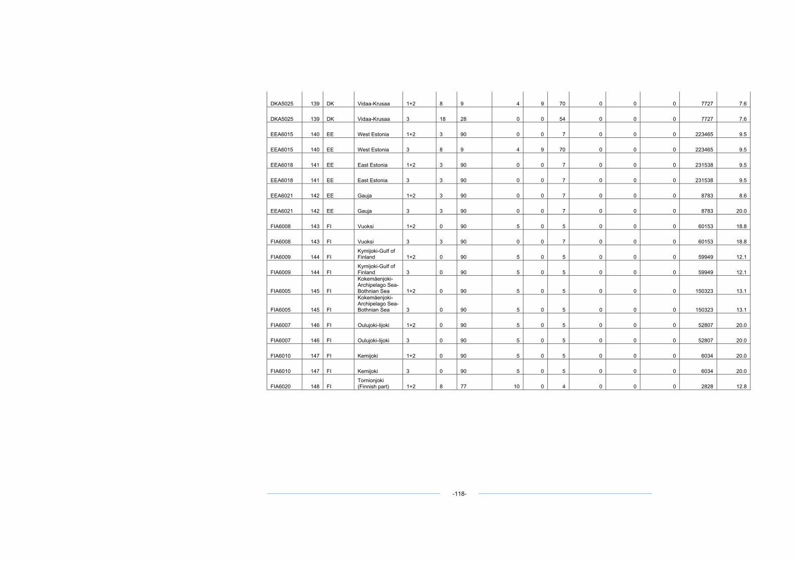
DKA5025 139 DK Vidaa-Krusaa 1+2 8 9 4 9 70 0 0 0 7727 7.6

DKA5025 139 DK Vidaa-Krusaa 3 18 28 0 0 54 0 0 0 7727 7.6

EEA6015 140 EE West Estonia 1+2 3 90 0 0 7 0 0 0 223465 9.5

EEA6015 140 EE West Estonia 3 8 9 4 9 70 0 0 0 223465 9.5

EEA6018 141 EE East Estonia 1+2 3 90 0 0 7 0 0 0 231538 9.5

EEA6018 141 EE East Estonia 3 3 90 0 0 7 0 0 0 231538 9.5

EEA6021 142 EE Gauja 1+2 3 90 0 0 7 0 0 0 8783 8.6

EEA6021 142 EE Gauja 3 3 90 0 0 7 0 0 0 8783 20.0

FIA6008 143 FI Vuoksi 1+2 0 90 5 0 5 0 0 0 60153 18.8

FIA6008 143 FI Vuoksi 3 3 90 0 0 7 0 0 0 60153 18.8

FIA6009 144 FI Kymijoki-Gulf of Finland 1+2 0 90 5 0 5 0 0 0 59949 12.1

FIA6009 144 FI Kymijoki-Gulf of Finland 3 0 90 5 0 5 0 0 0 59949 12.1

FIA6005 145 FI

Kokemäenjoki-Archipelago Sea-Bothnian Sea 1+2 0 90 5 0 5 0 0 0 150323 13.1

FIA6005 145 FI

Kokemäenjoki-Archipelago Sea-Bothnian Sea 3 0 90 5 0 5 0 0 0 150323 13.1

FIA6007 146 FI Oulujoki-Iijoki 1+2 0 90 5 0 5 0 0 0 52807 20.0

FIA6007 146 FI Oulujoki-Iijoki 3 0 90 5 0 5 0 0 0 52807 20.0

FIA6010 147 FI Kemijoki 1+2 0 90 5 0 5 0 0 0 6034 20.0

FIA6010 147 FI Kemijoki 3 0 90 5 0 5 0 0 0 6034 20.0

FIA6020 148 FI Tornionjoki (Finnish part) 1+2 8 77 10 0 4 0 0 0 2828 12.8

-118-

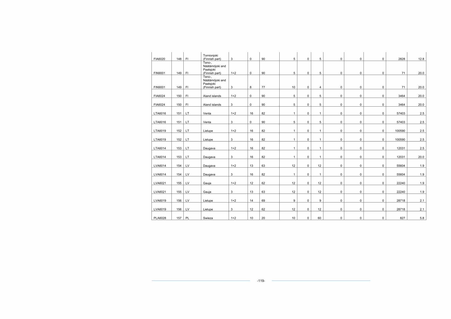
FIA6020 148 FI Tornionjoki (Finnish part) 3 0 90 5 0 5 0 0 0 2828 12.8

FIN9001 149 FI

Teno-, Näätämöjoki and Paatsjoki (Finnish part) 1+2 0 90 5 0 5 0 0 0 71 20.0

FIN9001 149 FI

Teno-, Näätämöjoki and Paatsjoki (Finnish part) 3 8 77 10 0 4 0 0 0 71 20.0

FIA6024 150 FI Aland islands 1+2 0 90 5 0 5 0 0 0 3464 20.0

FIA6024 150 FI Aland islands 3 0 90 5 0 5 0 0 0 3464 20.0

LTA6016 151 LT Venta 1+2 16 82 1 0 1 0 0 0 57403 2.5

LTA6016 151 LT Venta 3 0 90 5 0 5 0 0 0 57403 2.5

LTA6019 152 LT Lielupe 1+2 16 82 1 0 1 0 0 0 100590 2.5

LTA6019 152 LT Lielupe 3 16 82 1 0 1 0 0 0 100590 2.5

LTA6014 153 LT Daugava 1+2 16 82 1 0 1 0 0 0 12031 2.5

LTA6014 153 LT Daugava 3 16 82 1 0 1 0 0 0 12031 20.0

LVA6014 154 LV Daugava 1+2 13 63 12 0 12 0 0 0 55604 1.9

LVA6014 154 LV Daugava 3 16 82 1 0 1 0 0 0 55604 1.9

LVA6021 155 LV Gauja 1+2 12 62 12 0 12 0 0 0 22240 1.9

LVA6021 155 LV Gauja 3 13 63 12 0 12 0 0 0 22240 1.9

LVA6019 156 LV Lielupe 1+2 14 69 9 0 9 0 0 0 28718 2.1

LVA6019 156 LV Lielupe 3 12 62 12 0 12 0 0 0 28718 2.1

PLA6028 157 PL Swieza 1+2 10 20 10 0 60 0 0 0 827 5.8

-119-

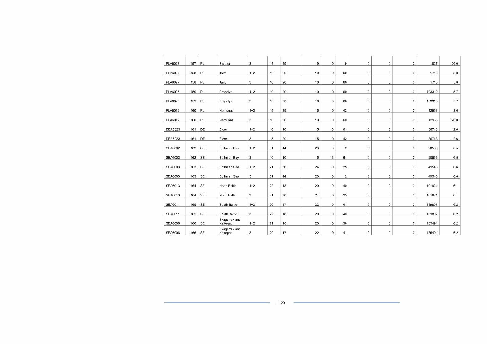
PLA6028 157 PL Swieza 3 14 69 9 0 9 0 0 0 827 20.0

PLA6027 158 PL Jarft 1+2 10 20 10 0 60 0 0 0 1716 5.8

PLA6027 158 PL Jarft 3 10 20 10 0 60 0 0 0 1716 5.8

PLA6025 159 PL Pregolya 1+2 10 20 10 0 60 0 0 0 103310 5.7

PLA6025 159 PL Pregolya 3 10 20 10 0 60 0 0 0 103310 5.7

PLA6012 160 PL Nemunas 1+2 15 29 15 0 42 0 0 0 12953 3.6

PLA6012 160 PL Nemunas 3 10 20 10 0 60 0 0 0 12953 20.0

DEA5023 161 DE Eider 1+2 10 10 5 13 61 0 0 0 36743 12.6

DEA5023 161 DE Eider 3 15 29 15 0 42 0 0 0 36743 12.6

SEA6002 162 SE Bothnian Bay 1+2 31 44 23 0 2 0 0 0 20566 6.5

SEA6002 162 SE Bothnian Bay 3 10 10 5 13 61 0 0 0 20566 6.5

SEA6003 163 SE Bothnian Sea 1+2 21 30 24 0 25 0 0 0 49546 6.6

SEA6003 163 SE Bothnian Sea 3 31 44 23 0 2 0 0 0 49546 6.6

SEA6013 164 SE North Baltic 1+2 22 18 20 0 40 0 0 0 101921 6.1

SEA6013 164 SE North Baltic 3 21 30 24 0 25 0 0 0 101921 6.1

SEA6011 165 SE South Baltic 1+2 20 17 22 0 41 0 0 0 139807 6.2

SEA6011 165 SE South Baltic 3 22 18 20 0 40 0 0 0 139807 6.2

SEA6006 166 SE Skagerrak and Kattegat 1+2 21 18 23 0 38 0 0 0 135491 6.2

SEA6006 166 SE Skagerrak and Kattegat 3 20 17 22 0 41 0 0 0 135491 6.2

-120-

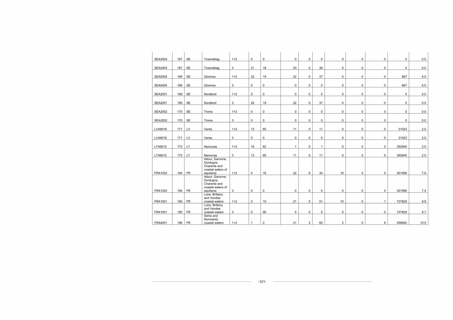
SEA2004 167 SE Troendelag 1+2 0 0 0 0 0 0 0 0 0 0.0

SEA2004 167 SE Troendelag 3 21 18 23 0 38 0 0 0 0 0.0

SEA5004 168 SE Glomma 1+2 22 19 22 0 37 0 0 0 667 6.0

SEA5004 168 SE Glomma 3 0 0 0 0 0 0 0 0 667 6.0

SEA2001 169 SE Nordland 1+2 0 0 0 0 0 0 0 0 0 0.0

SEA2001 169 SE Nordland 3 22 19 22 0 37 0 0 0 0 0.0

SEA2002 170 SE Troms 1+2 0 0 0 0 0 0 0 0 0 0.0

SEA2002 170 SE Troms 3 0 0 0 0 0 0 0 0 0 0.0

LVA6016 171 LV Venta 1+2 13 65 11 0 11 0 0 0 31023 2.0

LVA6016 171 LV Venta 3 0 0 0 0 0 0 0 0 31023 2.0

LTA6012 172 LT Nemunas 1+2 16 82 1 0 1 0 0 0 392945 2.5

LTA6012 172 LT Nemunas 3 13 65 11 0 11 0 0 0 392945 2.5

FRA1002 194 FR

Adour, Garonne, Dordogne, Charente and coastal waters of aquitania 1+2 4 16 22 6 34 18 0 0 301566 7.9

FRA1002 194 FR

Adour, Garonne, Dordogne, Charente and coastal waters of aquitania 3 0 0 0 0 0 0 0 0 301566 7.4

FRA1001 195 FR

Loire, Brittany and Vendee coastal waters 1+2 2 10 21 5 51 10 0 1 727829 9.9

FRA1001 195 FR

Loire, Brittany and Vendee coastal waters 3 0 90 5 0 5 0 0 0 727829 9.7

FRA4001 196 FR

Seine and Normandy coastal waters 1+2 1 2 21 2 65 2 0 6 456682 10.0

-121-

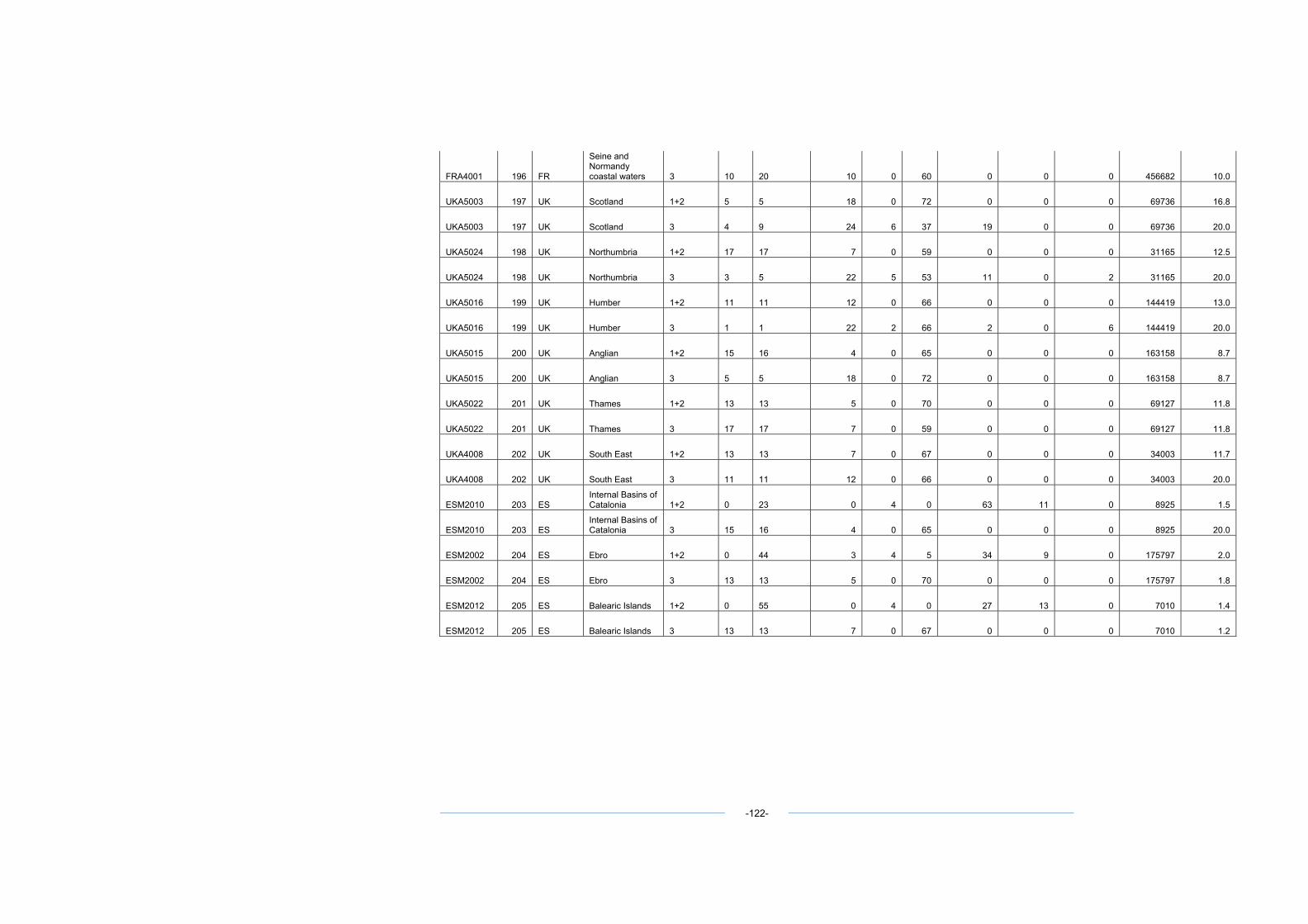
FRA4001 196 FR

Seine and Normandy coastal waters 3 10 20 10 0 60 0 0 0 456682 10.0

UKA5003 197 UK Scotland 1+2 5 5 18 0 72 0 0 0 69736 16.8

UKA5003 197 UK Scotland 3 4 9 24 6 37 19 0 0 69736 20.0

UKA5024 198 UK Northumbria 1+2 17 17 7 0 59 0 0 0 31165 12.5

UKA5024 198 UK Northumbria 3 3 5 22 5 53 11 0 2 31165 20.0

UKA5016 199 UK Humber 1+2 11 11 12 0 66 0 0 0 144419 13.0

UKA5016 199 UK Humber 3 1 1 22 2 66 2 0 6 144419 20.0

UKA5015 200 UK Anglian 1+2 15 16 4 0 65 0 0 0 163158 8.7

UKA5015 200 UK Anglian 3 5 5 18 0 72 0 0 0 163158 8.7

UKA5022 201 UK Thames 1+2 13 13 5 0 70 0 0 0 69127 11.8

UKA5022 201 UK Thames 3 17 17 7 0 59 0 0 0 69127 11.8

UKA4008 202 UK South East 1+2 13 13 7 0 67 0 0 0 34003 11.7

UKA4008 202 UK South East 3 11 11 12 0 66 0 0 0 34003 20.0

ESM2010 203 ES Internal Basins of Catalonia 1+2 0 23 0 4 0 63 11 0 8925 1.5

ESM2010 203 ES Internal Basins of Catalonia 3 15 16 4 0 65 0 0 0 8925 20.0

ESM2002 204 ES Ebro 1+2 0 44 3 4 5 34 9 0 175797 2.0

ESM2002 204 ES Ebro 3 13 13 5 0 70 0 0 0 175797 1.8

ESM2012 205 ES Balearic Islands 1+2 0 55 0 4 0 27 13 0 7010 1.4

ESM2012 205 ES Balearic Islands 3 13 13 7 0 67 0 0 0 7010 1.2

-122-

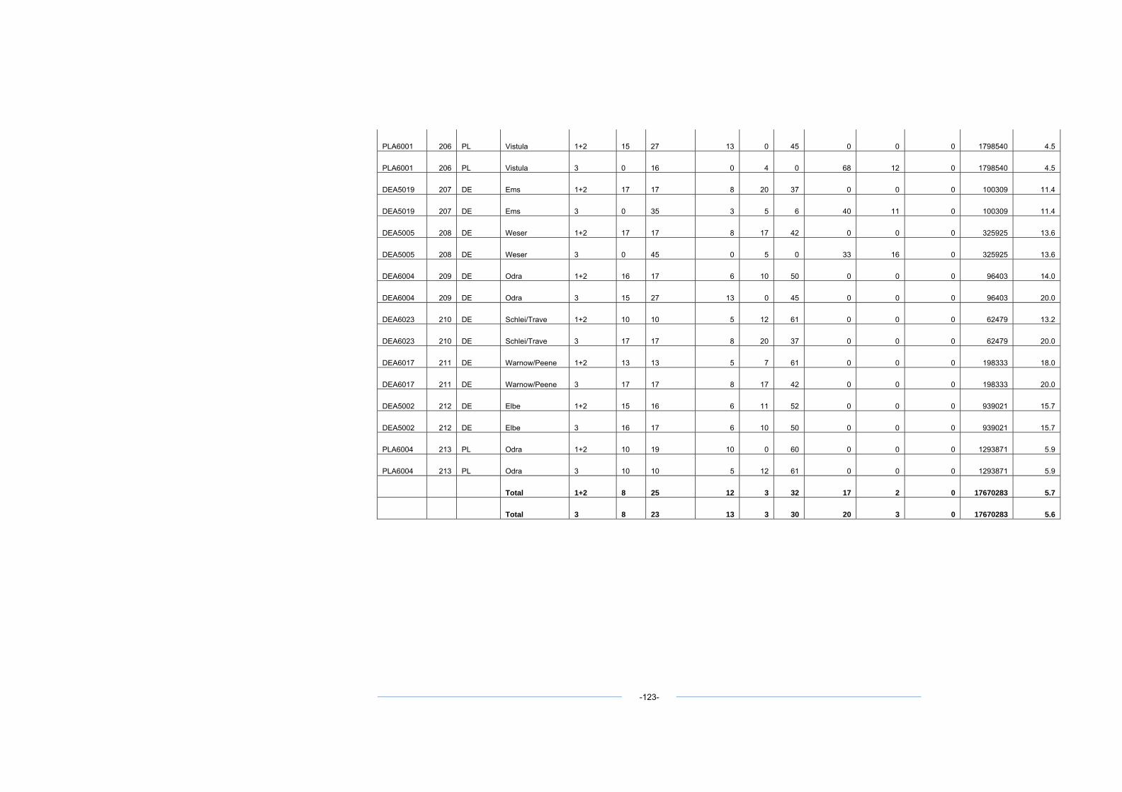
PLA6001 206 PL Vistula 1+2 15 27 13 0 45 0 0 0 1798540 4.5

PLA6001 206 PL Vistula 3 0 16 0 4 0 68 12 0 1798540 4.5

DEA5019 207 DE Ems 1+2 17 17 8 20 37 0 0 0 100309 11.4

DEA5019 207 DE Ems 3 0 35 3 5 6 40 11 0 100309 11.4

DEA5005 208 DE Weser 1+2 17 17 8 17 42 0 0 0 325925 13.6

DEA5005 208 DE Weser 3 0 45 0 5 0 33 16 0 325925 13.6

DEA6004 209 DE Odra 1+2 16 17 6 10 50 0 0 0 96403 14.0

DEA6004 209 DE Odra 3 15 27 13 0 45 0 0 0 96403 20.0

DEA6023 210 DE Schlei/Trave 1+2 10 10 5 12 61 0 0 0 62479 13.2

DEA6023 210 DE Schlei/Trave 3 17 17 8 20 37 0 0 0 62479 20.0

DEA6017 211 DE Warnow/Peene 1+2 13 13 5 7 61 0 0 0 198333 18.0

DEA6017 211 DE Warnow/Peene 3 17 17 8 17 42 0 0 0 198333 20.0

DEA5002 212 DE Elbe 1+2 15 16 6 11 52 0 0 0 939021 15.7

DEA5002 212 DE Elbe 3 16 17 6 10 50 0 0 0 939021 15.7

PLA6004 213 PL Odra 1+2 10 19 10 0 60 0 0 0 1293871 5.9

PLA6004 213 PL Odra 3 10 10 5 12 61 0 0 0 1293871 5.9

Total 1+2 8 25 12 3 32 17 2 0 17670283 5.7

Total 3 8 23 13 3 30 20 3 0 17670283 5.6

-123-

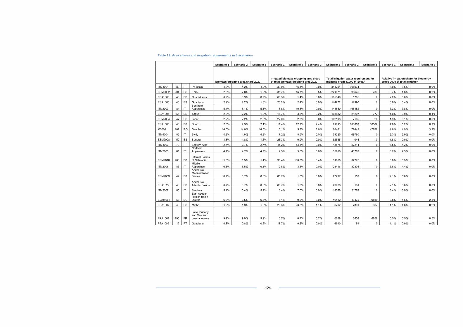
Table 19: Area shares and irrigation requirements in 3 scenarios

Scenario 1 Scenario 2 Scenario 3 Scenario 1 Scenario 2 Scenario 3 Scenario 1 Scenario 2 Scenario 3 Scenario 1 Scenario 2 Scenario 3

Biomass cropping area share 2020 Irrigated biomass croppnig area share of total biomass cropping area 2020


Relative irrigation share for bioenergy crops 2020 of total irrigation

ITM4001 80 IT Po Basin 4.2% 4.2% 4.2% 39.0% 46.1% 0.0% 311751 366634 0 3.0% 3.5% 0.0%

ESM2002 204 ES Ebro 2.0% 2.0% 1.8% 35.7% 16.7% 0.5% 221671 98675 733 3.7% 1.8% 0.0%

ESA1006 45 ES Guadalquivir 0.9% 0.9% 0.7% 68.3% 1.4% 0.0% 165340 1765 0 2.2% 0.0% 0.0%

ESA1005 46 ES Guadiana 2.2% 2.2% 1.8% 20.2% 2.4% 0.0% 144772 12990 0 3.6% 0.4% 0.0%

ITM2003 84 IT Southern Appenines 5.1% 5.1% 5.1% 8.8% 10.3% 0.0% 141650 166452 0 3.3% 3.8% 0.0%

ESA1004 51 ES Tagus 2.2% 2.2% 1.9% 16.7% 3.8% 0.2% 103882 21207 777 4.0% 0.9% 0.1%

ESM2004 47 ES Jucar 2.2% 2.2% 2.0% 27.0% 2.3% 0.0% 102198 7105 20 1.9% 0.1% 0.0%

ESA1003 43 ES Duero 2.3% 2.3% 2.1% 11.4% 12.9% 2.4% 91093 103063 16387 4.6% 5.2% 0.9%

M5001 109 RO Danube 14.0% 14.0% 14.0% 5.1% 5.3% 3.6% 68461 72442 47786 4.6% 4.9% 3.2%

ITM4004 86 IT Sicily 4.9% 4.9% 4.9% 7.2% 8.5% 0.0% 59325 69780 0 3.3% 3.9% 0.0%

ESM2008 50 ES Segura 1.8% 1.8% 1.6% 28.3% 0.9% 0.0% 52565 1045 0 1.8% 0.0% 0.0%

ITM4003 79 IT Eastern Alps 2.7% 2.7% 2.7% 45.2% 53.1% 0.0% 48678 57214 0 3.5% 4.2% 0.0%

ITM2005 81 IT Northern Appenines 4.7% 4.7% 4.7% 4.3% 5.0% 0.0% 35918 41789 0 3.7% 4.3% 0.0%

ESM2010 203 ES Internal Basins of Catalonia 1.5% 1.5% 1.4% 90.4% 100.0% 3.4% 31850 37275 0 3.0% 3.5% 0.0%

ITM2006 83 IT Middle Appenines 6.5% 6.5% 6.5% 2.8% 3.3% 0.0% 28416 32876 0 3.8% 4.4% 0.0%

ESM2009 42 ES

Andalusia Mediterranean Basins 0.7% 0.7% 0.6% 85.7% 1.0% 0.0% 27717 152 0 2.1% 0.0% 0.0%

ESA1029 40 ES Andalusia Atlantic Basins 0.7% 0.7% 0.6% 85.7% 1.0% 0.0% 23928 131 0 2.1% 0.0% 0.0%

ITM2007 85 IT Sardinia 5.4% 5.4% 5.4% 6.4% 7.5% 0.0% 18556 21778 0 3.4% 3.9% 0.0%

BGM4002 55 BG

East Aegean Region Basin District 6.5% 6.5% 6.5% 8.1% 9.5% 5.0% 16412 19475 9839 3.8% 4.5% 2.3%

ESA1007 48 ES Minho 1.9% 1.9% 1.8% 20.3% 23.8% 1.1% 6762 7891 367 4.1% 4.8% 0.2%

FRA1001 195 FR

Loire, Brittany and Vendee coastal waters 9.9% 9.9% 9.9% 0.7% 0.7% 0.7% 6658 6658 6658 0.5% 0.5% 0.5%

PTA1005 19 PT Guadiana 0.8% 0.8% 0.6% 18.7% 0.2% 0.0% 6540 51 0 1.1% 0.0% 0.0%

-124-

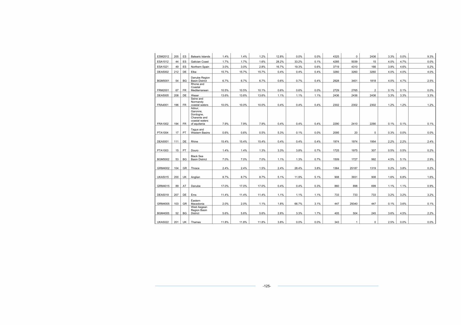
ESM2012 205 ES Balearic Islands 1.4% 1.4% 1.2% 12.8% 0.0% 0.0% 4325 0 2436 3.3% 0.0% 9.3%

ESA1012 44 ES Galician Coast 1.7% 1.7% 1.6% 28.2% 33.2% 0.1% 4285 5039 15 4.0% 4.7% 0.0%

ESA1021 49 ES Northern Spain 3.0% 3.0% 2.8% 16.7% 19.3% 0.6% 3719 4310 166 3.9% 4.6% 0.2%

DEA5002 212 DE Elbe 15.7% 15.7% 15.7% 0.4% 0.4% 0.4% 3260 3260 3260 4.0% 4.0% 4.0%

BGM5001 54 BG Danube Region Basin District 6.7% 6.7% 6.7% 0.6% 0.7% 0.4% 2928 3401 1818 4.0% 4.7% 2.5%

FRM2001 67 FR

Rhone and Coastal Mediterranean 10.5% 10.5% 10.1% 0.6% 0.6% 0.0% 2729 2765 2 0.1% 0.1% 0.0%

DEA5005 208 DE Weser 13.6% 13.6% 13.6% 1.1% 1.1% 1.1% 2436 2436 2436 3.3% 3.3% 3.3%

FRA4001 196 FR

Seine and Normandy coastal waters 10.0% 10.0% 10.0% 0.4% 0.4% 0.4% 2302 2302 2302 1.2% 1.2% 1.2%

FRA1002 194 FR

Adour, Garonne, Dordogne, Charente and coastal waters of aquitania 7.9% 7.9% 7.9% 0.4% 0.4% 0.4% 2290 2410 2290 0.1% 0.1% 0.1%

PTA1004 17 PT Tagus and Western Basins 0.6% 0.6% 0.5% 5.3% 0.1% 0.0% 2095 20 0 0.3% 0.0% 0.0%

DEA5001 111 DE Rhine 15.4% 15.4% 15.4% 0.4% 0.4% 0.4% 1974 1974 1954 2.2% 2.2% 2.4%

PTA1003 15 PT Douro 1.4% 1.4% 1.3% 3.3% 3.8% 0.7% 1725 1975 307 0.5% 0.5% 0.2%

BGM5002 53 BG Black Sea Basin District 7.0% 7.0% 7.0% 1.1% 1.3% 0.7% 1509 1727 992 4.5% 5.1% 2.9%

GRM4002 104 GR Thrace 2.4% 2.4% 1.5% 2.4% 28.4% 3.8% 1364 25187 1319 0.2% 3.8% 0.2%

UKA5015 200 UK Anglian 8.7% 8.7% 8.7% 5.1% 11.9% 5.1% 908 3931 908 1.6% 6.8% 1.6%

GRM4015 89 AT Danube 17.0% 17.0% 17.0% 0.4% 0.4% 0.3% 860 898 699 1.1% 1.1% 0.9%

DEA5019 207 DE Ems 11.4% 11.4% 11.4% 1.1% 1.1% 1.1% 733 733 733 3.2% 3.2% 3.2%

GRM4005 103 GR Eastern Macedonia 2.0% 2.0% 1.1% 1.8% 66.7% 3.1% 447 29340 447 0.1% 3.6% 0.1%

BGM4005 52 BG

West Aegean Region Basin District 5.6% 5.6% 5.6% 2.8% 3.3% 1.7% 405 504 245 3.6% 4.5% 2.2%

UKA5022 201 UK Thames 11.8% 11.8% 11.8% 3.8% 0.0% 0.0% 343 1 0 2.5% 0.0% 0.0%

-125-

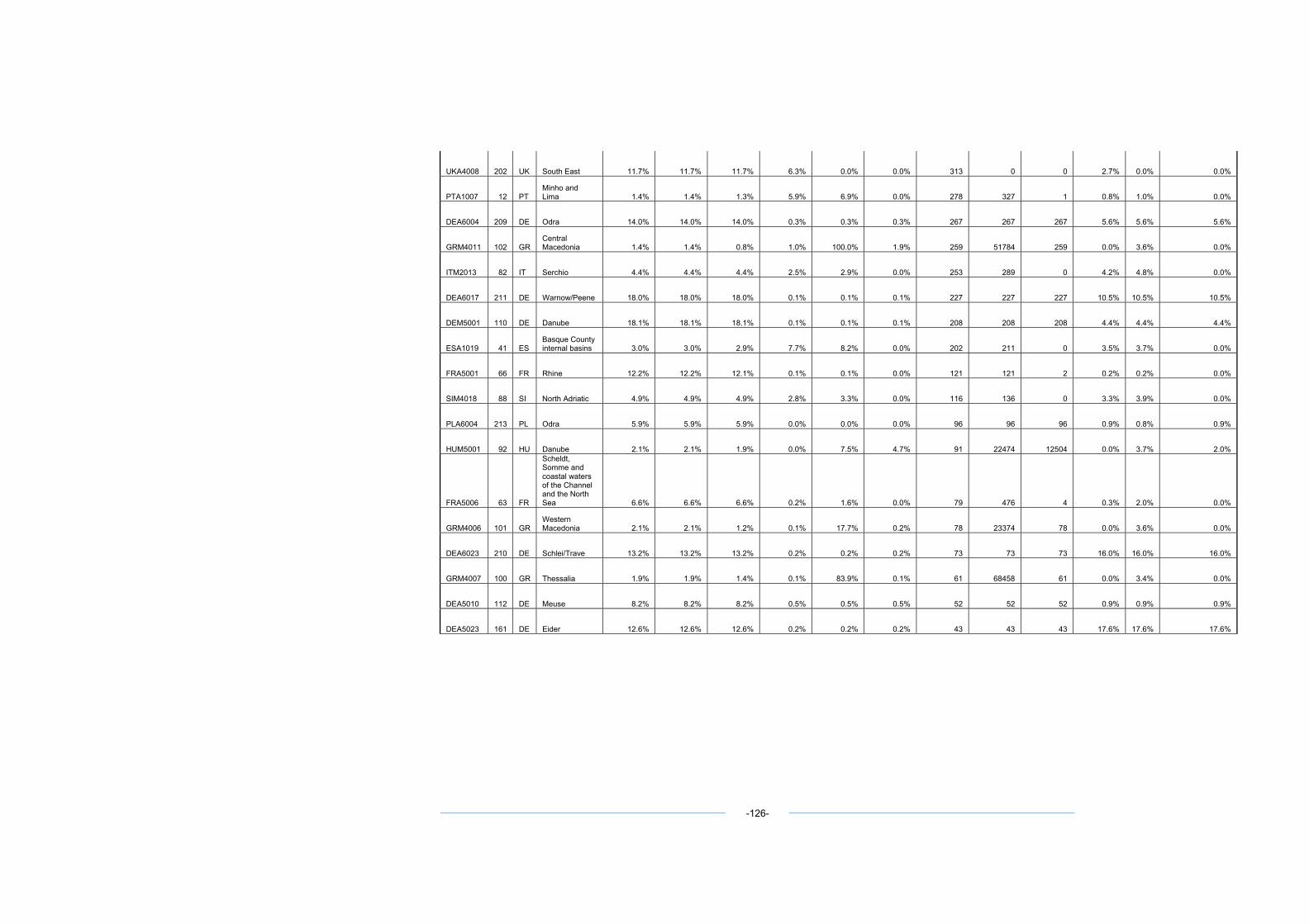
UKA4008 202 UK South East 11.7% 11.7% 11.7% 6.3% 0.0% 0.0% 313 0 0 2.7% 0.0% 0.0%

PTA1007 12 PT Minho and Lima 1.4% 1.4% 1.3% 5.9% 6.9% 0.0% 278 327 1 0.8% 1.0% 0.0%

DEA6004 209 DE Odra 14.0% 14.0% 14.0% 0.3% 0.3% 0.3% 267 267 267 5.6% 5.6% 5.6%

GRM4011 102 GR Central Macedonia 1.4% 1.4% 0.8% 1.0% 100.0% 1.9% 259 51784 259 0.0% 3.6% 0.0%

ITM2013 82 IT Serchio 4.4% 4.4% 4.4% 2.5% 2.9% 0.0% 253 289 0 4.2% 4.8% 0.0%

DEA6017 211 DE Warnow/Peene 18.0% 18.0% 18.0% 0.1% 0.1% 0.1% 227 227 227 10.5% 10.5% 10.5%

DEM5001 110 DE Danube 18.1% 18.1% 18.1% 0.1% 0.1% 0.1% 208 208 208 4.4% 4.4% 4.4%

ESA1019 41 ES Basque County internal basins 3.0% 3.0% 2.9% 7.7% 8.2% 0.0% 202 211 0 3.5% 3.7% 0.0%

FRA5001 66 FR Rhine 12.2% 12.2% 12.1% 0.1% 0.1% 0.0% 121 121 2 0.2% 0.2% 0.0%

SIM4018 88 SI North Adriatic 4.9% 4.9% 4.9% 2.8% 3.3% 0.0% 116 136 0 3.3% 3.9% 0.0%

PLA6004 213 PL Odra 5.9% 5.9% 5.9% 0.0% 0.0% 0.0% 96 96 96 0.9% 0.8% 0.9%

HUM5001 92 HU Danube 2.1% 2.1% 1.9% 0.0% 7.5% 4.7% 91 22474 12504 0.0% 3.7% 2.0%

FRA5006 63 FR

Scheldt, Somme and coastal waters of the Channel and the North Sea 6.6% 6.6% 6.6% 0.2% 1.6% 0.0% 79 476 4 0.3% 2.0% 0.0%

GRM4006 101 GR Western Macedonia 2.1% 2.1% 1.2% 0.1% 17.7% 0.2% 78 23374 78 0.0% 3.6% 0.0%

DEA6023 210 DE Schlei/Trave 13.2% 13.2% 13.2% 0.2% 0.2% 0.2% 73 73 73 16.0% 16.0% 16.0%

GRM4007 100 GR Thessalia 1.9% 1.9% 1.4% 0.1% 83.9% 0.1% 61 68458 61 0.0% 3.4% 0.0%

DEA5010 112 DE Meuse 8.2% 8.2% 8.2% 0.5% 0.5% 0.5% 52 52 52 0.9% 0.9% 0.9%

DEA5023 161 DE Eider 12.6% 12.6% 12.6% 0.2% 0.2% 0.2% 43 43 43 17.6% 17.6% 17.6%

-126-

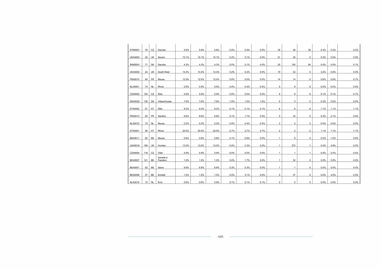
ATM5001 78 CZ Danube 5.8% 5.8% 5.8% 0.0% 0.0% 0.0% 39 39 39 0.3% 0.3% 0.3%

UKA4003 25 UK Severn 15.1% 15.1% 15.1% 0.2% 0.1% 0.0% 21 35 0 0.3% 0.5% 0.0%

SKM5001 71 SK Danube 4.3% 4.3% 4.3% 0.0% 0.1% 0.0% 20 100 64 0.0% 0.0% 0.1%

UKA4002 24 UK South West 14.4% 14.4% 14.4% 0.2% 0.2% 0.0% 19 32 0 3.2% 5.6% 0.0%

FRA5010 64 FR Meuse 12.5% 12.5% 12.5% 0.0% 0.0% 0.0% 14 14 0 0.6% 0.6% 0.1%

NLA5001 74 NL Rhine 0.5% 0.5% 0.5% 0.4% 0.4% 0.4% 9 9 9 0.0% 0.0% 0.0%

CZA5002 120 CZ Elbe 5.9% 5.9% 5.9% 0.0% 0.0% 0.0% 9 9 9 0.1% 0.1% 0.1%

DKA5025 139 DK Vidaa-Krusaa 7.6% 7.6% 7.6% 1.5% 1.5% 1.5% 6 0 0 0.3% 0.0% 0.0%

ATA5002 91 AT Elbe 9.2% 9.2% 9.2% 0.1% 0.1% 0.1% 6 6 6 1.1% 1.1% 1.1%

FRA5013 65 FR Sambre 6.6% 6.6% 6.6% 0.1% 1.7% 0.0% 5 33 0 0.3% 2.1% 0.0%

NLA5010 73 NL Meuse 0.2% 0.2% 0.2% 0.4% 0.4% 0.4% 2 2 2 0.0% 0.0% 0.0%

ATA5001 90 AT Rhine 20.0% 20.0% 20.0% 2.7% 2.7% 2.7% 2 2 2 1.1% 1.1% 1.1%

BEA5011 60 BE Meuse 0.8% 0.8% 0.8% 0.1% 0.6% 0.0% 1 6 0 0.2% 1.0% 0.0%

UKA5016 199 UK Humber 13.0% 13.0% 13.0% 0.0% 2.3% 0.0% 1 372 1 0.0% 4.8% 0.0%

CZA6004 118 CZ Oder 5.9% 5.9% 5.9% 0.0% 0.0% 0.0% 1 1 1 0.4% 0.4% 0.4%

BEA5007 121 BE Scheldt in Flanders 1.0% 1.0% 1.0% 0.0% 1.7% 0.0% 1 32 0 0.0% 0.9% 0.0%

BEA4001 62 BE Seine 6.8% 6.8% 6.8% 0.3% 0.3% 0.0% 1 1 0 0.5% 0.5% 0.0%

BEA5008 57 BE Scheldt 1.5% 1.5% 1.5% 0.0% 3.1% 0.0% 0 37 0 0.0% 4.0% 0.0%

NLA5019 72 NL Ems 0.6% 0.6% 0.6% 0.1% 0.1% 0.1% 0 0 0 0.0% 0.0% 0.0%

-127-

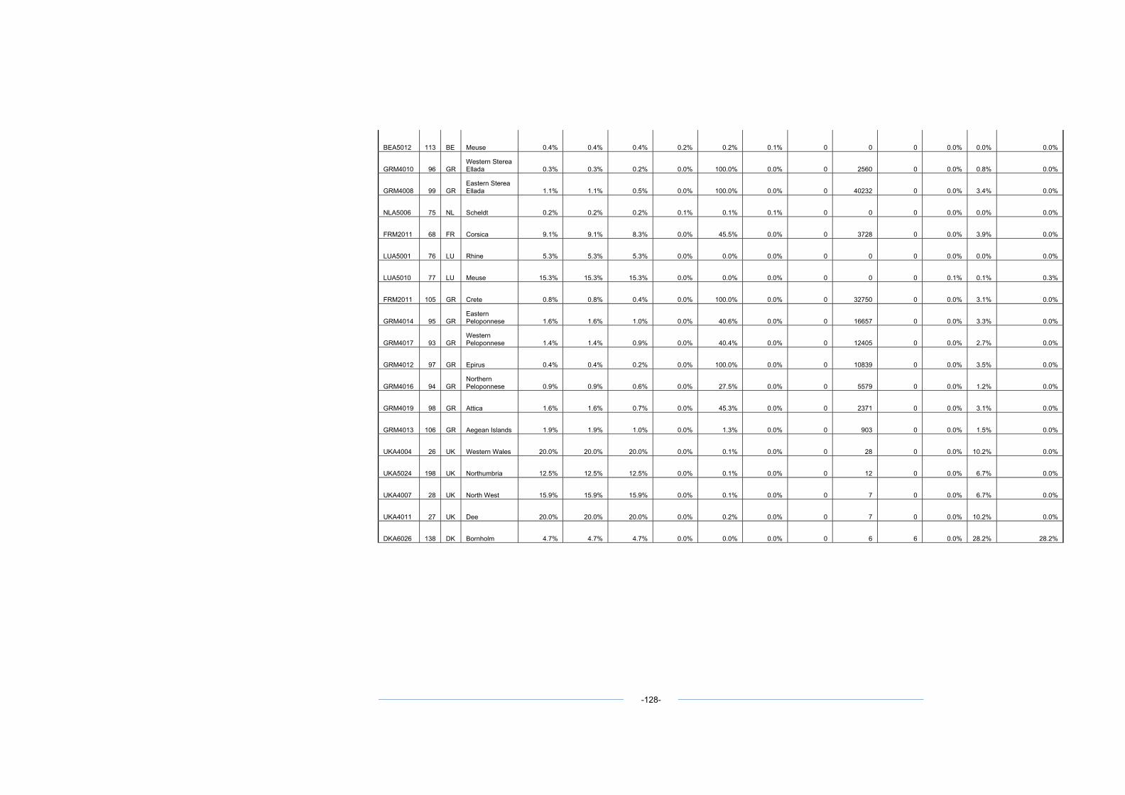
BEA5012 113 BE Meuse 0.4% 0.4% 0.4% 0.2% 0.2% 0.1% 0 0 0 0.0% 0.0% 0.0%

GRM4010 96 GR Western Sterea Ellada 0.3% 0.3% 0.2% 0.0% 100.0% 0.0% 0 2560 0 0.0% 0.8% 0.0%

GRM4008 99 GR Eastern Sterea Ellada 1.1% 1.1% 0.5% 0.0% 100.0% 0.0% 0 40232 0 0.0% 3.4% 0.0%

NLA5006 75 NL Scheldt 0.2% 0.2% 0.2% 0.1% 0.1% 0.1% 0 0 0 0.0% 0.0% 0.0%

FRM2011 68 FR Corsica 9.1% 9.1% 8.3% 0.0% 45.5% 0.0% 0 3728 0 0.0% 3.9% 0.0%

LUA5001 76 LU Rhine 5.3% 5.3% 5.3% 0.0% 0.0% 0.0% 0 0 0 0.0% 0.0% 0.0%

LUA5010 77 LU Meuse 15.3% 15.3% 15.3% 0.0% 0.0% 0.0% 0 0 0 0.1% 0.1% 0.3%

FRM2011 105 GR Crete 0.8% 0.8% 0.4% 0.0% 100.0% 0.0% 0 32750 0 0.0% 3.1% 0.0%

GRM4014 95 GR Eastern Peloponnese 1.6% 1.6% 1.0% 0.0% 40.6% 0.0% 0 16657 0 0.0% 3.3% 0.0%

GRM4017 93 GR Western Peloponnese 1.4% 1.4% 0.9% 0.0% 40.4% 0.0% 0 12405 0 0.0% 2.7% 0.0%

GRM4012 97 GR Epirus 0.4% 0.4% 0.2% 0.0% 100.0% 0.0% 0 10839 0 0.0% 3.5% 0.0%

GRM4016 94 GR Northern Peloponnese 0.9% 0.9% 0.6% 0.0% 27.5% 0.0% 0 5579 0 0.0% 1.2% 0.0%

GRM4019 98 GR Attica 1.6% 1.6% 0.7% 0.0% 45.3% 0.0% 0 2371 0 0.0% 3.1% 0.0%

GRM4013 106 GR Aegean Islands 1.9% 1.9% 1.0% 0.0% 1.3% 0.0% 0 903 0 0.0% 1.5% 0.0%

UKA4004 26 UK Western Wales 20.0% 20.0% 20.0% 0.0% 0.1% 0.0% 0 28 0 0.0% 10.2% 0.0%

UKA5024 198 UK Northumbria 12.5% 12.5% 12.5% 0.0% 0.1% 0.0% 0 12 0 0.0% 6.7% 0.0%

UKA4007 28 UK North West 15.9% 15.9% 15.9% 0.0% 0.1% 0.0% 0 7 0 0.0% 6.7% 0.0%

UKA4011 27 UK Dee 20.0% 20.0% 20.0% 0.0% 0.2% 0.0% 0 7 0 0.0% 10.2% 0.0%

DKA6026 138 DK Bornholm 4.7% 4.7% 4.7% 0.0% 0.0% 0.0% 0 6 6 0.0% 28.2% 28.2%

-128-

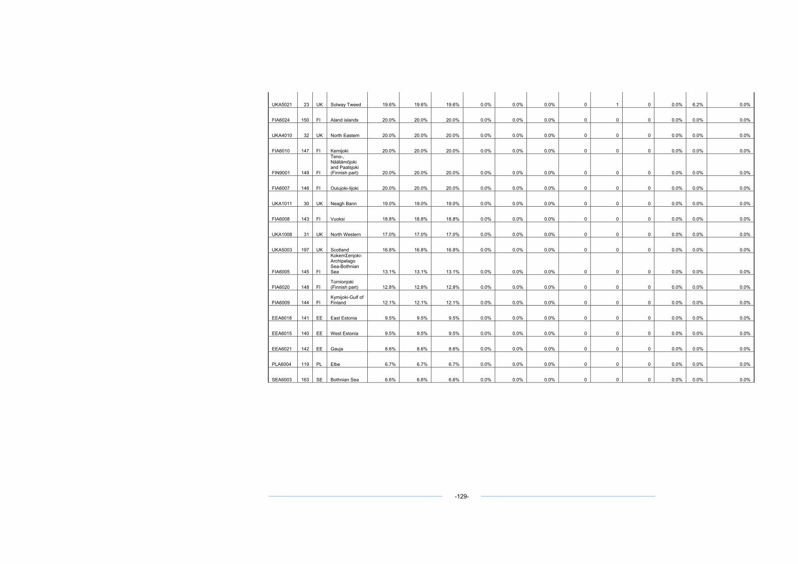
UKA5021 23 UK Solway Tweed 19.6% 19.6% 19.6% 0.0% 0.0% 0.0% 0 1 0 0.0% 6.2% 0.0%

FIA6024 150 FI Aland islands 20.0% 20.0% 20.0% 0.0% 0.0% 0.0% 0 0 0 0.0% 0.0% 0.0%

UKA4010 32 UK North Eastern 20.0% 20.0% 20.0% 0.0% 0.0% 0.0% 0 0 0 0.0% 0.0% 0.0%

FIA6010 147 FI Kemijoki 20.0% 20.0% 20.0% 0.0% 0.0% 0.0% 0 0 0 0.0% 0.0% 0.0%

FIN9001 149 FI

Teno-, Näätämöjoki and Paatsjoki (Finnish part) 20.0% 20.0% 20.0% 0.0% 0.0% 0.0% 0 0 0 0.0% 0.0% 0.0%

FIA6007 146 FI Oulujoki-Iijoki 20.0% 20.0% 20.0% 0.0% 0.0% 0.0% 0 0 0 0.0% 0.0% 0.0%

UKA1011 30 UK Neagh Bann 19.0% 19.0% 19.0% 0.0% 0.0% 0.0% 0 0 0 0.0% 0.0% 0.0%

FIA6008 143 FI Vuoksi 18.8% 18.8% 18.8% 0.0% 0.0% 0.0% 0 0 0 0.0% 0.0% 0.0%

UKA1008 31 UK North Western 17.0% 17.0% 17.0% 0.0% 0.0% 0.0% 0 0 0 0.0% 0.0% 0.0%

UKA5003 197 UK Scotland 16.8% 16.8% 16.8% 0.0% 0.0% 0.0% 0 0 0 0.0% 0.0% 0.0%

FIA6005 145 FI

KokemΣenjoki-Archipelago Sea-Bothnian Sea 13.1% 13.1% 13.1% 0.0% 0.0% 0.0% 0 0 0 0.0% 0.0% 0.0%

FIA6020 148 FI Tornionjoki (Finnish part) 12.8% 12.8% 12.8% 0.0% 0.0% 0.0% 0 0 0 0.0% 0.0% 0.0%

FIA6009 144 FI Kymijoki-Gulf of Finland 12.1% 12.1% 12.1% 0.0% 0.0% 0.0% 0 0 0 0.0% 0.0% 0.0%

EEA6018 141 EE East Estonia 9.5% 9.5% 9.5% 0.0% 0.0% 0.0% 0 0 0 0.0% 0.0% 0.0%

EEA6015 140 EE West Estonia 9.5% 9.5% 9.5% 0.0% 0.0% 0.0% 0 0 0 0.0% 0.0% 0.0%

EEA6021 142 EE Gauja 8.6% 8.6% 8.6% 0.0% 0.0% 0.0% 0 0 0 0.0% 0.0% 0.0%

PLA6004 119 PL Elbe 6.7% 6.7% 6.7% 0.0% 0.0% 0.0% 0 0 0 0.0% 0.0% 0.0%

SEA6003 163 SE Bothnian Sea 6.6% 6.6% 6.6% 0.0% 0.0% 0.0% 0 0 0 0.0% 0.0% 0.0%

-129-

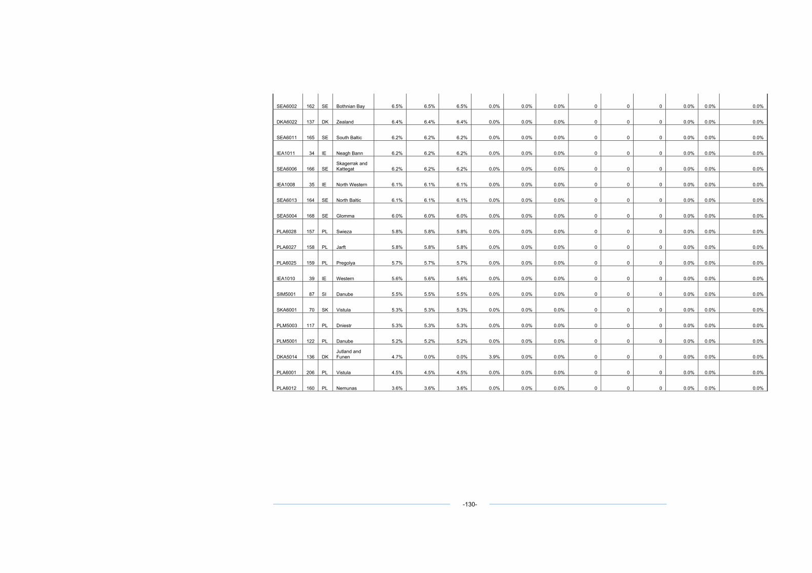
SEA6002 162 SE Bothnian Bay 6.5% 6.5% 6.5% 0.0% 0.0% 0.0% 0 0 0 0.0% 0.0% 0.0%

DKA6022 137 DK Zealand 6.4% 6.4% 6.4% 0.0% 0.0% 0.0% 0 0 0 0.0% 0.0% 0.0%

SEA6011 165 SE South Baltic 6.2% 6.2% 6.2% 0.0% 0.0% 0.0% 0 0 0 0.0% 0.0% 0.0%

IEA1011 34 IE Neagh Bann 6.2% 6.2% 6.2% 0.0% 0.0% 0.0% 0 0 0 0.0% 0.0% 0.0%

SEA6006 166 SE Skagerrak and Kattegat 6.2% 6.2% 6.2% 0.0% 0.0% 0.0% 0 0 0 0.0% 0.0% 0.0%

IEA1008 35 IE North Western 6.1% 6.1% 6.1% 0.0% 0.0% 0.0% 0 0 0 0.0% 0.0% 0.0%

SEA6013 164 SE North Baltic 6.1% 6.1% 6.1% 0.0% 0.0% 0.0% 0 0 0 0.0% 0.0% 0.0%

SEA5004 168 SE Glomma 6.0% 6.0% 6.0% 0.0% 0.0% 0.0% 0 0 0 0.0% 0.0% 0.0%

PLA6028 157 PL Swieza 5.8% 5.8% 5.8% 0.0% 0.0% 0.0% 0 0 0 0.0% 0.0% 0.0%

PLA6027 158 PL Jarft 5.8% 5.8% 5.8% 0.0% 0.0% 0.0% 0 0 0 0.0% 0.0% 0.0%

PLA6025 159 PL Pregolya 5.7% 5.7% 5.7% 0.0% 0.0% 0.0% 0 0 0 0.0% 0.0% 0.0%

IEA1010 39 IE Western 5.6% 5.6% 5.6% 0.0% 0.0% 0.0% 0 0 0 0.0% 0.0% 0.0%

SIM5001 87 SI Danube 5.5% 5.5% 5.5% 0.0% 0.0% 0.0% 0 0 0 0.0% 0.0% 0.0%

SKA6001 70 SK Vistula 5.3% 5.3% 5.3% 0.0% 0.0% 0.0% 0 0 0 0.0% 0.0% 0.0%

PLM5003 117 PL Dniestr 5.3% 5.3% 5.3% 0.0% 0.0% 0.0% 0 0 0 0.0% 0.0% 0.0%

PLM5001 122 PL Danube 5.2% 5.2% 5.2% 0.0% 0.0% 0.0% 0 0 0 0.0% 0.0% 0.0%

DKA5014 136 DK Jutland and Funen 4.7% 0.0% 0.0% 3.9% 0.0% 0.0% 0 0 0 0.0% 0.0% 0.0%

PLA6001 206 PL Vistula 4.5% 4.5% 4.5% 0.0% 0.0% 0.0% 0 0 0 0.0% 0.0% 0.0%

PLA6012 160 PL Nemunas 3.6% 3.6% 3.6% 0.0% 0.0% 0.0% 0 0 0 0.0% 0.0% 0.0%

-130-

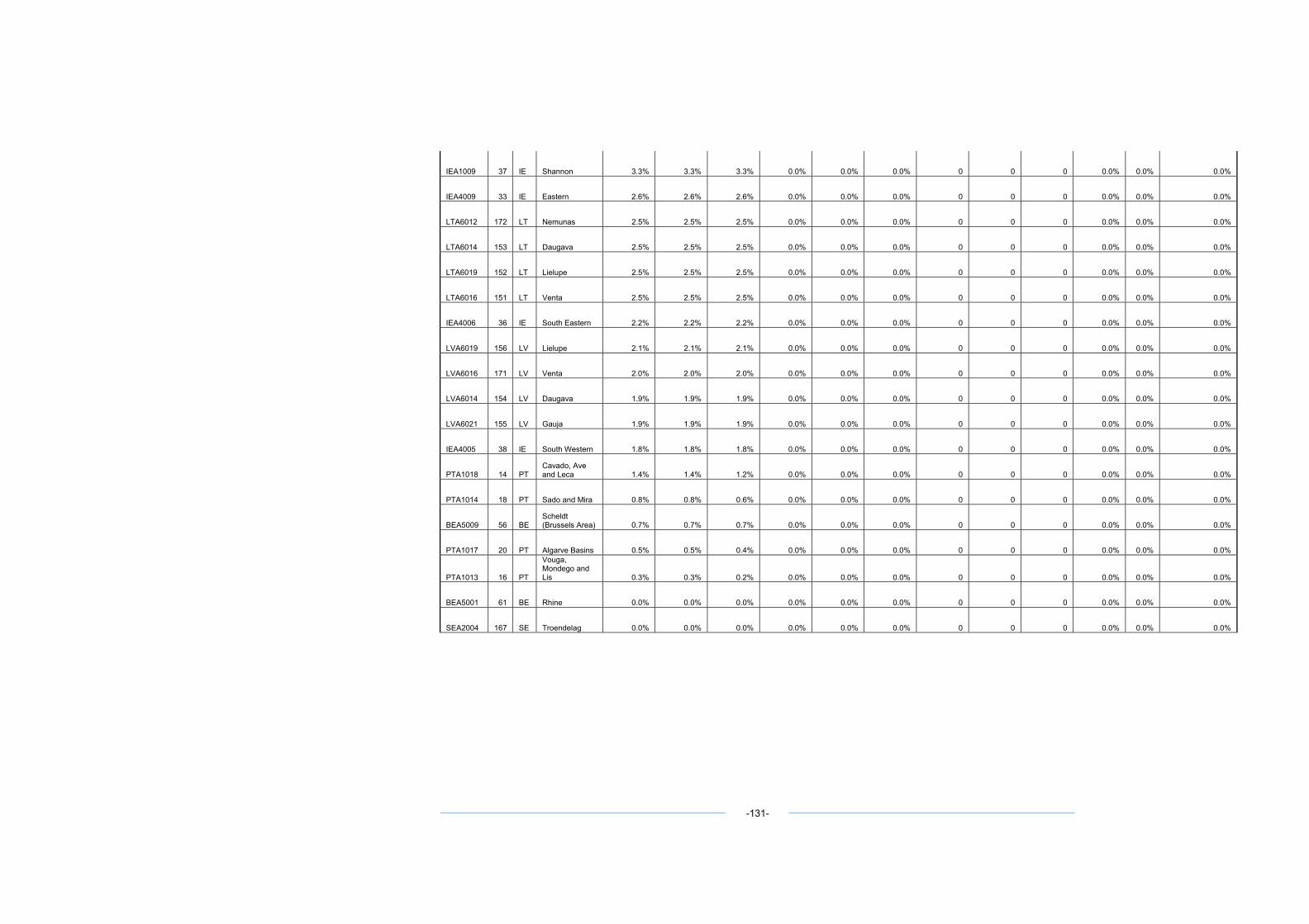
IEA1009 37 IE Shannon 3.3% 3.3% 3.3% 0.0% 0.0% 0.0% 0 0 0 0.0% 0.0% 0.0%

IEA4009 33 IE Eastern 2.6% 2.6% 2.6% 0.0% 0.0% 0.0% 0 0 0 0.0% 0.0% 0.0%

LTA6012 172 LT Nemunas 2.5% 2.5% 2.5% 0.0% 0.0% 0.0% 0 0 0 0.0% 0.0% 0.0%

LTA6014 153 LT Daugava 2.5% 2.5% 2.5% 0.0% 0.0% 0.0% 0 0 0 0.0% 0.0% 0.0%

LTA6019 152 LT Lielupe 2.5% 2.5% 2.5% 0.0% 0.0% 0.0% 0 0 0 0.0% 0.0% 0.0%

LTA6016 151 LT Venta 2.5% 2.5% 2.5% 0.0% 0.0% 0.0% 0 0 0 0.0% 0.0% 0.0%

IEA4006 36 IE South Eastern 2.2% 2.2% 2.2% 0.0% 0.0% 0.0% 0 0 0 0.0% 0.0% 0.0%

LVA6019 156 LV Lielupe 2.1% 2.1% 2.1% 0.0% 0.0% 0.0% 0 0 0 0.0% 0.0% 0.0%

LVA6016 171 LV Venta 2.0% 2.0% 2.0% 0.0% 0.0% 0.0% 0 0 0 0.0% 0.0% 0.0%

LVA6014 154 LV Daugava 1.9% 1.9% 1.9% 0.0% 0.0% 0.0% 0 0 0 0.0% 0.0% 0.0%

LVA6021 155 LV Gauja 1.9% 1.9% 1.9% 0.0% 0.0% 0.0% 0 0 0 0.0% 0.0% 0.0%

IEA4005 38 IE South Western 1.8% 1.8% 1.8% 0.0% 0.0% 0.0% 0 0 0 0.0% 0.0% 0.0%

PTA1018 14 PT Cavado, Ave and Leca 1.4% 1.4% 1.2% 0.0% 0.0% 0.0% 0 0 0 0.0% 0.0% 0.0%

PTA1014 18 PT Sado and Mira 0.8% 0.8% 0.6% 0.0% 0.0% 0.0% 0 0 0 0.0% 0.0% 0.0%

BEA5009 56 BE Scheldt (Brussels Area) 0.7% 0.7% 0.7% 0.0% 0.0% 0.0% 0 0 0 0.0% 0.0% 0.0%

PTA1017 20 PT Algarve Basins 0.5% 0.5% 0.4% 0.0% 0.0% 0.0% 0 0 0 0.0% 0.0% 0.0%

PTA1013 16 PT

Vouga, Mondego and Lis 0.3% 0.3% 0.2% 0.0% 0.0% 0.0% 0 0 0 0.0% 0.0% 0.0%

BEA5001 61 BE Rhine 0.0% 0.0% 0.0% 0.0% 0.0% 0.0% 0 0 0 0.0% 0.0% 0.0%

SEA2004 167 SE Troendelag 0.0% 0.0% 0.0% 0.0% 0.0% 0.0% 0 0 0 0.0% 0.0% 0.0%

-131-

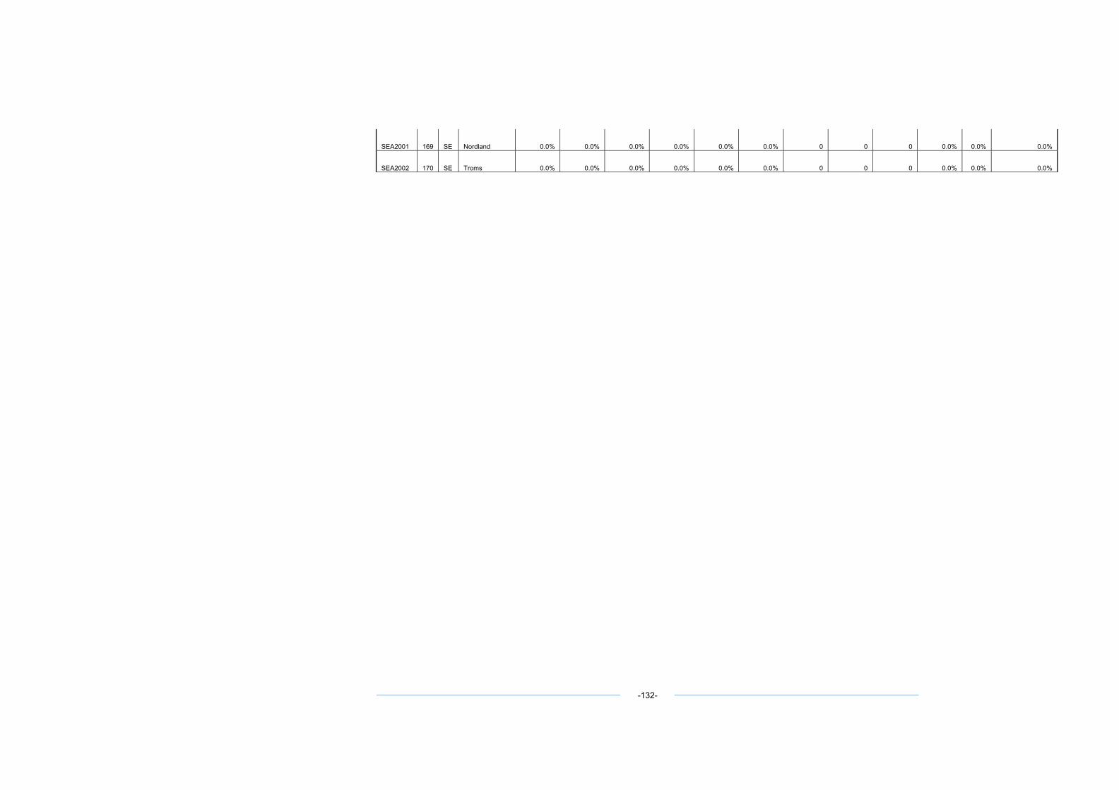
SEA2001 169 SE Nordland 0.0% 0.0% 0.0% 0.0% 0.0% 0.0% 0 0 0 0.0% 0.0% 0.0%

SEA2002 170 SE Troms 0.0% 0.0% 0.0% 0.0% 0.0% 0.0% 0 0 0 0.0% 0.0% 0.0%

-132-

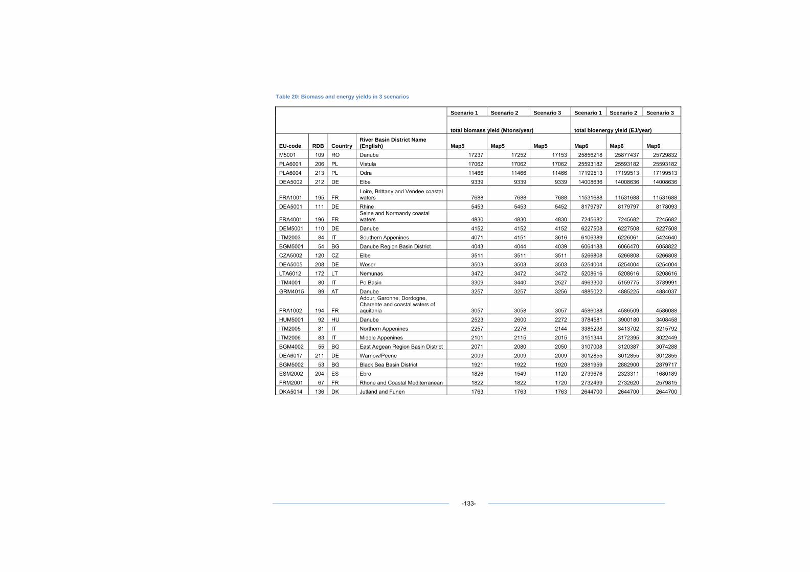
Table 20: Biomass and energy yields in 3 scenarios

Scenario 1 Scenario 2 Scenario 3 Scenario 1 Scenario 2 Scenario 3

total biomass yield (Mtons/year) total bioenergy yield (EJ/year)

EU-code RDB Country River Basin District Name (English) Map5 Map5 Map5 Map6 Map6 Map6

M5001 109 RO Danube 17237 17252 17153 25856218 25877437 25729832 PLA6001 206 PL Vistula 17062 17062 17062 25593182 25593182 25593182 PLA6004 213 PL Odra 11466 11466 11466 17199513 17199513 17199513 DEA5002 212 DE Elbe 9339 9339 9339 14008636 14008636 14008636

FRA1001 195 FR Loire, Brittany and Vendee coastal waters 7688 7688 7688 11531688 11531688 11531688

DEA5001 111 DE Rhine 5453 5453 5452 8179797 8179797 8178093

FRA4001 196 FR Seine and Normandy coastal waters 4830 4830 4830 7245682 7245682 7245682

DEM5001 110 DE Danube 4152 4152 4152 6227508 6227508 6227508 ITM2003 84 IT Southern Appenines 4071 4151 3616 6106389 6226061 5424640 BGM5001 54 BG Danube Region Basin District 4043 4044 4039 6064188 6066470 6058822 CZA5002 120 CZ Elbe 3511 3511 3511 5266808 5266808 5266808 DEA5005 208 DE Weser 3503 3503 3503 5254004 5254004 5254004 LTA6012 172 LT Nemunas 3472 3472 3472 5208616 5208616 5208616 ITM4001 80 IT Po Basin 3309 3440 2527 4963300 5159775 3789991 GRM4015 89 AT Danube 3257 3257 3256 4885022 4885225 4884037

FRA1002 194 FR

Adour, Garonne, Dordogne, Charente and coastal waters of aquitania 3057 3058 3057 4586088 4586509 4586088

HUM5001 92 HU Danube 2523 2600 2272 3784581 3900180 3408458 ITM2005 81 IT Northern Appenines 2257 2276 2144 3385238 3413702 3215792 ITM2006 83 IT Middle Appenines 2101 2115 2015 3151344 3172395 3022449 BGM4002 55 BG East Aegean Region Basin District 2071 2080 2050 3107008 3120387 3074288 DEA6017 211 DE Warnow/Peene 2009 2009 2009 3012855 3012855 3012855 BGM5002 53 BG Black Sea Basin District 1921 1922 1920 2881959 2882900 2879717 ESM2002 204 ES Ebro 1826 1549 1120 2739676 2323311 1680189 FRM2001 67 FR Rhone and Coastal Mediterranean 1822 1822 1720 2732499 2732620 2579815 DKA5014 136 DK Jutland and Funen 1763 1763 1763 2644700 2644700 2644700

-133-

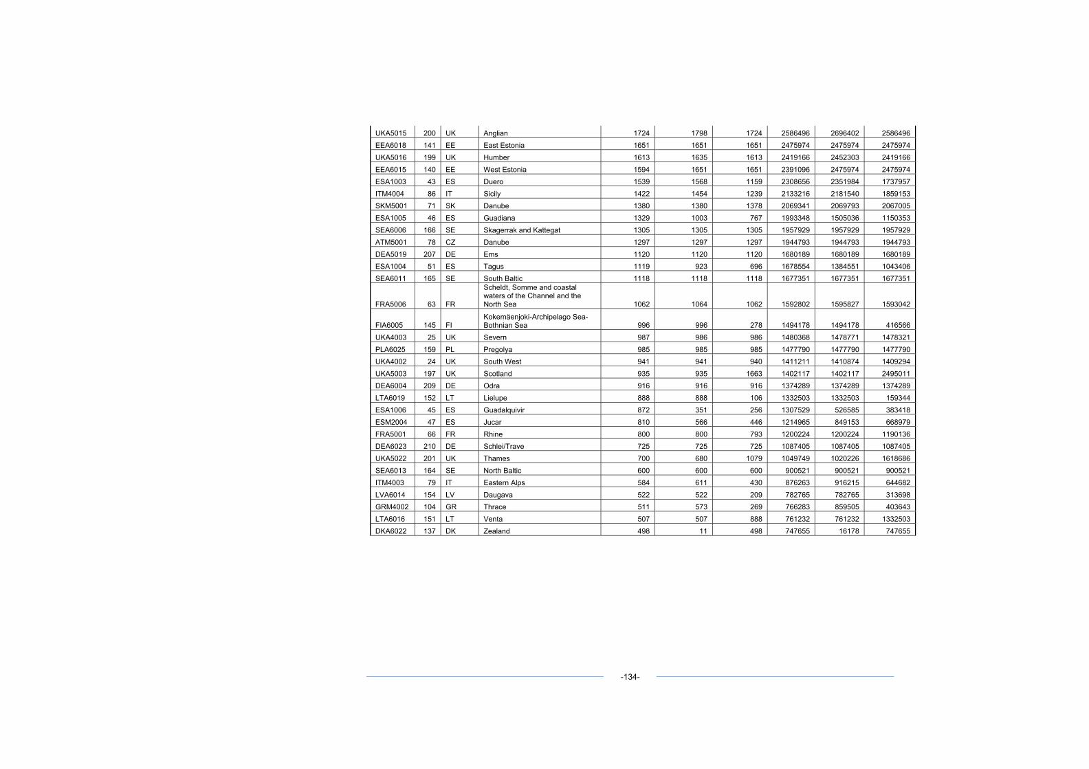
UKA5015 200 UK Anglian 1724 1798 1724 2586496 2696402 2586496 EEA6018 141 EE East Estonia 1651 1651 1651 2475974 2475974 2475974 UKA5016 199 UK Humber 1613 1635 1613 2419166 2452303 2419166 EEA6015 140 EE West Estonia 1594 1651 1651 2391096 2475974 2475974 ESA1003 43 ES Duero 1539 1568 1159 2308656 2351984 1737957 ITM4004 86 IT Sicily 1422 1454 1239 2133216 2181540 1859153 SKM5001 71 SK Danube 1380 1380 1378 2069341 2069793 2067005 ESA1005 46 ES Guadiana 1329 1003 767 1993348 1505036 1150353 SEA6006 166 SE Skagerrak and Kattegat 1305 1305 1305 1957929 1957929 1957929 ATM5001 78 CZ Danube 1297 1297 1297 1944793 1944793 1944793 DEA5019 207 DE Ems 1120 1120 1120 1680189 1680189 1680189 ESA1004 51 ES Tagus 1119 923 696 1678554 1384551 1043406 SEA6011 165 SE South Baltic 1118 1118 1118 1677351 1677351 1677351

FRA5006 63 FR

Scheldt, Somme and coastal waters of the Channel and the North Sea 1062 1064 1062 1592802 1595827 1593042

FIA6005 145 FI Kokemäenjoki-Archipelago Sea-Bothnian Sea 996 996 278 1494178 1494178 416566

UKA4003 25 UK Severn 987 986 986 1480368 1478771 1478321 PLA6025 159 PL Pregolya 985 985 985 1477790 1477790 1477790 UKA4002 24 UK South West 941 941 940 1411211 1410874 1409294 UKA5003 197 UK Scotland 935 935 1663 1402117 1402117 2495011 DEA6004 209 DE Odra 916 916 916 1374289 1374289 1374289 LTA6019 152 LT Lielupe 888 888 106 1332503 1332503 159344 ESA1006 45 ES Guadalquivir 872 351 256 1307529 526585 383418 ESM2004 47 ES Jucar 810 566 446 1214965 849153 668979 FRA5001 66 FR Rhine 800 800 793 1200224 1200224 1190136 DEA6023 210 DE Schlei/Trave 725 725 725 1087405 1087405 1087405 UKA5022 201 UK Thames 700 680 1079 1049749 1020226 1618686 SEA6013 164 SE North Baltic 600 600 600 900521 900521 900521 ITM4003 79 IT Eastern Alps 584 611 430 876263 916215 644682 LVA6014 154 LV Daugava 522 522 209 782765 782765 313698 GRM4002 104 GR Thrace 511 573 269 766283 859505 403643 LTA6016 151 LT Venta 507 507 888 761232 761232 1332503 DKA6022 137 DK Zealand 498 11 498 747655 16178 747655

-134-

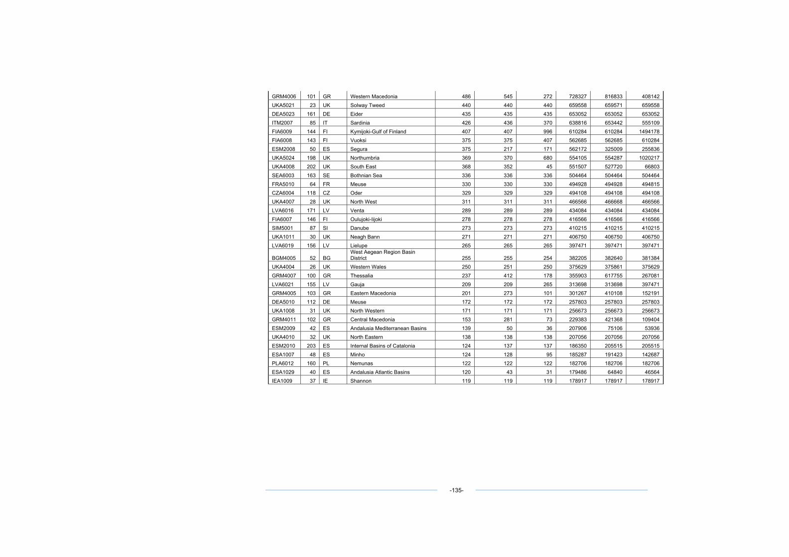
GRM4006 101 GR Western Macedonia 486 545 272 728327 816833 408142 UKA5021 23 UK Solway Tweed 440 440 440 659558 659571 659558 DEA5023 161 DE Eider 435 435 435 653052 653052 653052 ITM2007 85 IT Sardinia 426 436 370 638816 653442 555109 FIA6009 144 FI Kymijoki-Gulf of Finland 407 407 996 610284 610284 1494178 FIA6008 143 FI Vuoksi 375 375 407 562685 562685 610284 ESM2008 50 ES Segura 375 217 171 562172 325009 255836 UKA5024 198 UK Northumbria 369 370 680 554105 554287 1020217 UKA4008 202 UK South East 368 352 45 551507 527720 66803 SEA6003 163 SE Bothnian Sea 336 336 336 504464 504464 504464 FRA5010 64 FR Meuse 330 330 330 494928 494928 494815 CZA6004 118 CZ Oder 329 329 329 494108 494108 494108 UKA4007 28 UK North West 311 311 311 466566 466668 466566 LVA6016 171 LV Venta 289 289 289 434084 434084 434084 FIA6007 146 FI Oulujoki-Iijoki 278 278 278 416566 416566 416566 SIM5001 87 SI Danube 273 273 273 410215 410215 410215 UKA1011 30 UK Neagh Bann 271 271 271 406750 406750 406750 LVA6019 156 LV Lielupe 265 265 265 397471 397471 397471

BGM4005 52 BG West Aegean Region Basin District 255 255 254 382205 382640 381384

UKA4004 26 UK Western Wales 250 251 250 375629 375861 375629 GRM4007 100 GR Thessalia 237 412 178 355903 617755 267081 LVA6021 155 LV Gauja 209 209 265 313698 313698 397471 GRM4005 103 GR Eastern Macedonia 201 273 101 301267 410108 152191 DEA5010 112 DE Meuse 172 172 172 257803 257803 257803 UKA1008 31 UK North Western 171 171 171 256673 256673 256673 GRM4011 102 GR Central Macedonia 153 281 73 229383 421368 109404 ESM2009 42 ES Andalusia Mediterranean Basins 139 50 36 207906 75106 53936 UKA4010 32 UK North Eastern 138 138 138 207056 207056 207056 ESM2010 203 ES Internal Basins of Catalonia 124 137 137 186350 205515 205515 ESA1007 48 ES Minho 124 128 95 185287 191423 142687 PLA6012 160 PL Nemunas 122 122 122 182706 182706 182706 ESA1029 40 ES Andalusia Atlantic Basins 120 43 31 179486 64840 46564 IEA1009 37 IE Shannon 119 119 119 178917 178917 178917

-135-

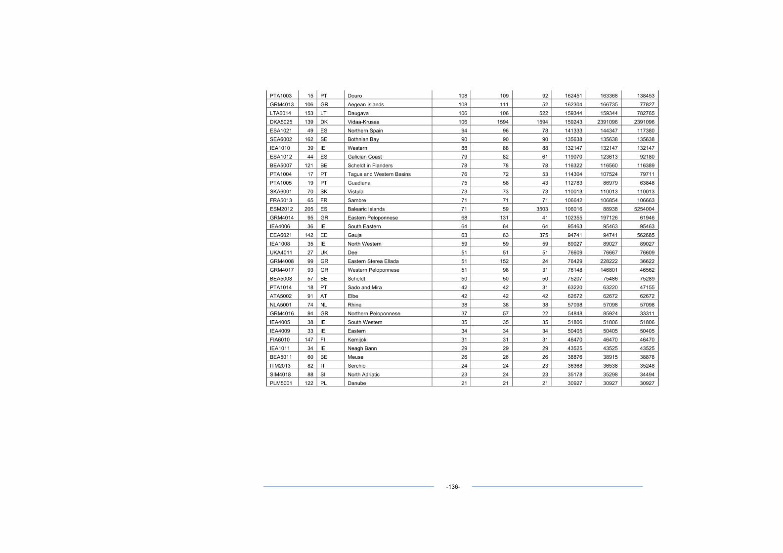
PTA1003 15 PT Douro 108 109 92 162451 163368 138453 GRM4013 106 GR Aegean Islands 108 111 52 162304 166735 77827 LTA6014 153 LT Daugava 106 106 522 159344 159344 782765 DKA5025 139 DK Vidaa-Krusaa 106 1594 1594 159243 2391096 2391096 ESA1021 49 ES Northern Spain 94 96 78 141333 144347 117380 SEA6002 162 SE Bothnian Bay 90 90 90 135638 135638 135638 IEA1010 39 IE Western 88 88 88 132147 132147 132147 ESA1012 44 ES Galician Coast 79 82 61 119070 123613 92180 BEA5007 121 BE Scheldt in Flanders 78 78 78 116322 116560 116389 PTA1004 17 PT Tagus and Western Basins 76 72 53 114304 107524 79711 PTA1005 19 PT Guadiana 75 58 43 112783 86979 63848 SKA6001 70 SK Vistula 73 73 73 110013 110013 110013 FRA5013 65 FR Sambre 71 71 71 106642 106854 106663 ESM2012 205 ES Balearic Islands 71 59 3503 106016 88938 5254004 GRM4014 95 GR Eastern Peloponnese 68 131 41 102355 197126 61946 IEA4006 36 IE South Eastern 64 64 64 95463 95463 95463 EEA6021 142 EE Gauja 63 63 375 94741 94741 562685 IEA1008 35 IE North Western 59 59 59 89027 89027 89027 UKA4011 27 UK Dee 51 51 51 76609 76667 76609 GRM4008 99 GR Eastern Sterea Ellada 51 152 24 76429 228222 36622 GRM4017 93 GR Western Peloponnese 51 98 31 76148 146801 46562 BEA5008 57 BE Scheldt 50 50 50 75207 75486 75289 PTA1014 18 PT Sado and Mira 42 42 31 63220 63220 47155 ATA5002 91 AT Elbe 42 42 42 62672 62672 62672 NLA5001 74 NL Rhine 38 38 38 57098 57098 57098 GRM4016 94 GR Northern Peloponnese 37 57 22 54848 85924 33311 IEA4005 38 IE South Western 35 35 35 51806 51806 51806 IEA4009 33 IE Eastern 34 34 34 50405 50405 50405 FIA6010 147 FI Kemijoki 31 31 31 46470 46470 46470 IEA1011 34 IE Neagh Bann 29 29 29 43525 43525 43525 BEA5011 60 BE Meuse 26 26 26 38876 38915 38878 ITM2013 82 IT Serchio 24 24 23 36368 36538 35248 SIM4018 88 SI North Adriatic 23 24 23 35178 35298 34494 PLM5001 122 PL Danube 21 21 21 30927 30927 30927

-136-

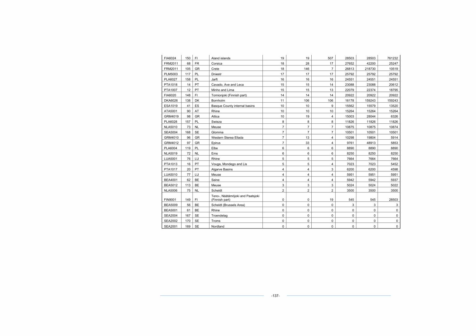
-137-

FIA6024 150 FI Aland islands 19 19 507 28503 28503 761232 FRM2011 68 FR Corsica 18 28 17 27652 42200 25247 FRM2011 105 GR Crete 18 146 7 26813 218730 10519 PLM5003 117 PL Dniestr 17 17 17 25792 25792 25792 PLA6027 158 PL Jarft 16 16 16 24551 24551 24551 PTA1018 14 PT Cavado, Ave and Leca 15 15 14 23088 23088 20612 PTA1007 12 PT Minho and Lima 15 15 13 22079 22374 18795 FIA6020 148 FI Tornionjoki (Finnish part) 14 14 14 20922 20922 20922 DKA6026 138 DK Bornholm 11 106 106 16178 159243 159243 ESA1019 41 ES Basque County internal basins 10 10 9 15562 15579 13520 ATA5001 90 AT Rhine 10 10 10 15264 15264 15264 GRM4019 98 GR Attica 10 19 4 15003 28044 6326 PLA6028 157 PL Swieza 8 8 8 11826 11826 11826 NLA5010 73 NL Meuse 7 7 7 10875 10875 10874 SEA5004 168 SE Glomma 7 7 7 10501 10501 10501 GRM4010 96 GR Western Sterea Ellada 7 13 4 10298 19804 5914 GRM4012 97 GR Epirus 7 33 4 9761 48913 5853 PLA6004 119 PL Elbe 6 6 6 8890 8890 8890 NLA5019 72 NL Ems 6 6 6 8250 8250 8250 LUA5001 76 LU Rhine 5 5 5 7664 7664 7664 PTA1013 16 PT Vouga, Mondego and Lis 5 5 4 7023 7023 5452 PTA1017 20 PT Algarve Basins 4 4 3 6200 6200 4598 LUA5010 77 LU Meuse 4 4 4 5951 5951 5951 BEA4001 62 BE Seine 4 4 4 5942 5942 5937 BEA5012 113 BE Meuse 3 3 3 5024 5024 5022 NLA5006 75 NL Scheldt 2 2 2 3500 3500 3500

FIN9001 149 FI Teno-, Näätämöjoki and Paatsjoki (Finnish part) 0 0 19 545 545 28503

BEA5009 56 BE Scheldt (Brussels Area) 0 0 0 3 3 3 BEA5001 61 BE Rhine 0 0 0 0 0 0 SEA2004 167 SE Troendelag 0 0 0 0 0 0 SEA2002 170 SE Troms 0 0 0 0 0 0

SEA2001 169 SE Nordland 0 0 0 0 0 0

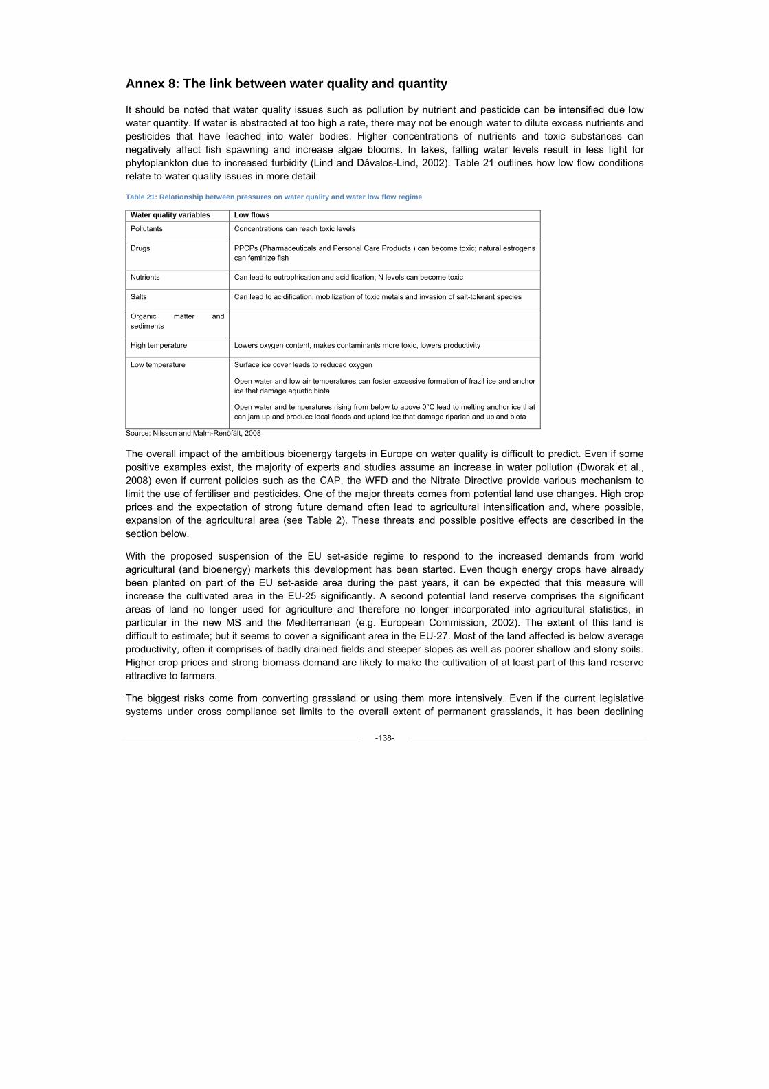
-138-

Annex 8: The link between water quality and quantity

It should be noted that water quality issues such as pollution by nutrient and pesticide can be intensified due low water quantity. If water is abstracted at too high a rate, there may not be enough water to dilute excess nutrients and pesticides that have leached into water bodies. Higher concentrations of nutrients and toxic substances can negatively affect fish spawning and increase algae blooms. In lakes, falling water levels result in less light for phytoplankton due to increased turbidity (Lind and Dávalos-Lind, 2002). Table 21 outlines how low flow conditions relate to water quality issues in more detail:

Table 21: Relationship between pressures on water quality and water low flow regime

Water quality variables Low flows

Pollutants Concentrations can reach toxic levels

Drugs PPCPs (Pharmaceuticals and Personal Care Products ) can become toxic; natural estrogens can feminize fish

Nutrients Can lead to eutrophication and acidification; N levels can become toxic

Salts Can lead to acidification, mobilization of toxic metals and invasion of salt-tolerant species

Organic matter and sediments

High temperature Lowers oxygen content, makes contaminants more toxic, lowers productivity

Low temperature Surface ice cover leads to reduced oxygen

Open water and low air temperatures can foster excessive formation of frazil ice and anchor ice that damage aquatic biota

Open water and temperatures rising from below to above 0°C lead to melting anchor ice that can jam up and produce local floods and upland ice that damage riparian and upland biota

Source: Nilsson and Malm-Renöfält, 2008

The overall impact of the ambitious bioenergy targets in Europe on water quality is difficult to predict. Even if some positive examples exist, the majority of experts and studies assume an increase in water pollution (Dworak et al., 2008) even if current policies such as the CAP, the WFD and the Nitrate Directive provide various mechanism to limit the use of fertiliser and pesticides. One of the major threats comes from potential land use changes. High crop prices and the expectation of strong future demand often lead to agricultural intensification and, where possible, expansion of the agricultural area (see Table 2). These threats and possible positive effects are described in the section below.

With the proposed suspension of the EU set-aside regime to respond to the increased demands from world agricultural (and bioenergy) markets this development has been started. Even though energy crops have already been planted on part of the EU set-aside area during the past years, it can be expected that this measure will increase the cultivated area in the EU-25 significantly. A second potential land reserve comprises the significant areas of land no longer used for agriculture and therefore no longer incorporated into agricultural statistics, in particular in the new MS and the Mediterranean (e.g. European Commission, 2002). The extent of this land is difficult to estimate; but it seems to cover a significant area in the EU-27. Most of the land affected is below average productivity, often it comprises of badly drained fields and steeper slopes as well as poorer shallow and stony soils. Higher crop prices and strong biomass demand are likely to make the cultivation of at least part of this land reserve attractive to farmers.

The biggest risks come from converting grassland or using them more intensively. Even if the current legislative systems under cross compliance set limits to the overall extent of permanent grasslands, it has been declining

-139-

gradually for several decades20. Several factors, including afforestation, the intensification of livestock farming, development of sites for housing, etc. play an essential role in this process. With regard to bioenergy cropping a conversion of permanent grassland through ploughing would pose significant water protection problems. Initially, there is a massive release of nutrients (and soil carbon) following the decomposition of the considerable quantity of organic matter in the upper layers of the soil. In addition turning grassland into arable land can drastically increase soil erosion rates depending on the cropping patterns and management, leading to higher surface run-off of nutrients to surface waters. The 2006 EEA bioenergy potential study, which was also considered when estimating the future land release, expects that a substantial amount of grassland (several million hectares) will be taken out of use in the period to 2030. The chances of converting these into bioenergy cropping area will then increase significantly.

Further the use of grassland, which is no longer needed for dairy cattle production due to the recent policy changes21, becomes more attractive become intensified. In particular nutrient emissions might increase as grass production for biogas has to increase. On the other side, manure use will decrease. In particular the new EU

countries, which still have vast areas of well‐managed grasslands, might be effected by intensification and

conversions to cropping land under influence of economic forces induced by increased globalisation and a high demands for cereals and bioenergy (Bioheritage, 2008).

However on the positive side the introduction of innovative bioenergy crops (such as perennials) and biomass cropping systems (such as double cropping) can in some cases lead to an extensification of land use They can add to crop diversity and combine a high yield with lower environmental pressures (lower input use), when compared to intensive food farming systems. Perennial bioenergy crops and short rotation forestry generally have less impact on: soil erosion and compaction, nutrient inputs into ground and surface water and pesticide pollution (European Environment Agency, 2007). Research examples show that biofuels derived from low-input high-diversity (LIHD) mixtures of native grassland perennials can provide more usable energy, greater greenhouse gas reductions, and less agrichemical pollution per hectare than can corn grain ethanol or soybean biodiesel. High-diversity grasslands had increasingly higher bioenergy yields that were 238% greater than monoculture yields after a decade (Tilman et al., 2006).

20 The current system allows a loss of 10% of ‘permanent pastures’ at national or regional level (which can mean almost complete loss in the most vulnerable areas), and also allows for the ‘offset’ of semi-natural biodiversity and carbon rich grasslands by a similar area of artificial grass cover on arable land. 21 Under CAP health check (see Official Journal of the European Union, L 30, Volume 52 of 31 January 2009) milk quotas will expire by April 2015. A 'soft landing' is ensured by increasing quotas by 1% every year between 2009/10 and 2013/14. For Italy, the 5% increase will be introduced immediately in 2009/10. In 2009/10 and 2010/11, farmers who exceed their milk quotas by more than 6% will have to pay a levy 50% higher than the normal penalty.

2009 Bioenergy

Documents

Transcript of 2009 Bioenergy