2007:220 CIV

M A S T E R ' S T H E S I S

Undermatching Butt Weldsin High Strength Steel

Svante Törnblom

Luleå University of Technology

MSc Programmes in Engineering Civil and mining Engineering

Department of Civil and Environmental EngineeringDivision of Structural Engineering

2007:220 CIV - ISSN: 1402-1617 - ISRN: LTU-EX--07/220--SE

PREFACE

Preface

This is the beginning of the end of a journey that started about five years ago. In the middle of August in 2002 I packed all my belongings into a model -72 Volvo 142 that I had inherited from my grandfather. The 1000 km trip from Gotland to Luleå was a good way to see Sweden at a moderate pace (the car wouldn’t go faster than 90 km/h) and to prepare myself mentally for the coming life as a student. At this stage I did not know where this journey would end, all I knew was that I had been accepted to an open engineering programme which would give me a master’s degree. Today, I’m fairly sure that the end of the journey will be a master’s degree in civil engineering, where this thesis is the final document. This work was initiated by Ramböll Sverige AB. SSAB Oxelösund financed the project and supplied material, welding, testing equipment and knowledge. I would like to express my gratitude to the persons who made this work possible. At first I would like to thank Professor Peter Collin who drafted me and gave me the opportunity to present this thesis in cooperation between Ramböll and LTU. I would also like to thank Daniel Stemne, at SSAB Oxelösund, who sacrificed his time to make me understand aspects of welding in high-strength steel. Thanks to Professor Bernt Johansson, who has listened to me and given me useful advice. Mats Fried and Simo Hietala, at SSAB Oxelösund, have done a magnificent job, welding and fabricating the test specimens and later testing them until fracture. A special thanks to my classmates. There have been many fruitful discussions, both related and non-related to school, during our “fika-” breaks. Finally, Lena, thank you for all the help and support at home when I was trying to finish this thesis off during some sunny/rainy summer weeks. Luleå, September 2007

Svante Törnblom

i

ABSTRACT

Abstract

The last years improvements in steel making technologies have resulted in steel grades with higher tensile strength, hardness, weldability etc. compared to conventional construction steel. This category steel gives lighter and smaller sized structures and cost reductions. Since the weld metal is still only a cast alloy whose strength mainly depends on its chemical composition, the differences in mechanical properties between the base plate and the consumable are increasing. The question is how to choose the undermatching level between the base plate and weld metal without compromising the global strength of the joint. In this master’s thesis, the effects of different weld geometries on the mechanical properties of undermatched welds in high strength quenched and tempered steel, are studied. Different undermatching levels have been accomplished by combining two different steels; Weldox 960 and Weldox 1100 together with two consumables; Filarc PZ6145 and Filarc PZ6149. Two methods have been used to gather information; 30 test specimens have been manufactured and tested at SSAB’s plant in Oxelösund and previous studies in this field have been analyzed in a literature review. Three different parameters were chosen to be studied in the laboratory tests, only one parameter was changed at a time:

• Width- to thickness relation • Undermatching • Relative thickness

The hypothesis was that if the weld metal is softer than the adjacent steel, it will yield before the base metal does. When the weld starts to deform, this deformation is constrained by the non-yielded surrounding metal. Tension is developed in both the width- and thickness directions, in addition to tension in the longitudinal direction due to the applied load. When the weld experiences tension in two or three material directions, the mean stress or hydrostatic stress in the weld is increased. As the hydrostatic stress is increased, by constraint, the magnitudes of the deviatoric stresses, which govern yielding, are reduced. This results in a stronger weld where increases in the applied load can be achieved. When the width- to thickness relation was studied, five different specimen widths, from 6 mm to 96 mm, were created out of the same plate. All specimens were taken from the same coupon which means that the welding parameters were identical for all specimens. In this case the effect of the width was obvious; the ultimate strength of the joint increased from 1070 MPa (6 mm) to 1192 MPa (96 mm). The ultimate strength of the weld metal was, in this case, 1015 MPa. When it comes to undermatching, all test specimens in Weldox 960 steel, welded with the stronger electrode, fractured in the base metal. This in spite of that the ratio between the weld metal’s and base metal’s yield strengths was as low as 0,77. In other literature only 15 % undermatching is recommended to achieve the full base metal strength in a joint. Only two different relative thicknesses could be accomplished. It was still obvious that the joint with a large weld volume had a lower strength than the one with a smaller volume.

ii

SAMMANFATTNING

Sammanfattning

De senaste årens förbättringar i ståltillverkningsindustrin har gett stålkvaliteter med högre hållfasthet, hårdhet, svetsbarhet etc. jämfört med konventionella konstruktionsstål. Den här sortens stål ger lättare och mindre konstruktioner och kostnadsminskningar. Eftersom svetsgodset fortfarande enbart är en legering, vars hållfasthet i huvudsak beror på dess kemiska sammansättning, ökar skillnaderna i mekaniska egenskaper mellan grundplåt och tillsatsmaterial. Frågan är, således, hur man väljer matchningsgrad mellan tillsatsmaterial och grundplåt utan att avsevärt minska den globala hållfastheten i förbandet. I det här examensarbetet undersöks vilken inverkan olika svetsgeometrier har på de mekaniska egenskaperna hos undermatchade svetsar i höghållfasta, seghärdade konstruktionsstål. Olika undermatchningsgrader har åstadkommits genom att kombinera två olika stål; Weldox 960 och Weldox 1100, tillsammans med två olika tillsatsmaterial; Filarc PZ 6145 och Filarc PZ 6149. Två olika metoder har använts för att samla information; dels har 30 stycken provkroppar tillverkats och dragits sönder hos SSAB i Oxelösund och dels har tidigare undersökningar inom detta område studerats i en litteraturstudie. Tre olika parametrar valdes ut för undersökning i de praktiska testerna, enbart en parameter ändrades åt gången:

• Sambandet mellan provstavsbredd och plåttjocklek • Undermatchningsgrad • Relativ tjocklek (förhållande mellan svetsgodsets bredd och plåttjockleken)

Hypotesen var att om svetsgodset är mjukare än kringliggande plåt kommer det att börja flyta innan grundmaterialet gör det. Då svetsen börjar deformeras, hindras denna deformation av att kringliggande material inte flyter. Dragspänningar utvecklas i svetsens tjockleks- och längsriktingar utöver den spänning som finns i lastriktningen. När svetsen påverkas av dragspänningar i fler än två riktningar ökar medelspänningen eller den hydrostatiska spänningen. Då den hydrostatiska spänningen ökar, p.g.a inspänning, minskar de deviatoriska spänningarna som styr flytgränsen. Detta ger en starkare svets som kan belastas mer. Då sambandet mellan provstavsbredd och plåttjocklek utreddes tillverkades fem olika provstavsbredder från 6 mm till 96 mm, ur samma plåt. Alla prov togs ur samma svetskupong, d.v.s. att svetsparametrarna var identiska för de olika proven. Här kunde breddens inverkan tydligt påvisas; förbandets brotthållfasthet ökade från 1070 MPa (6mm) till 1192 MPa (96mm). Brottgränsen för svetsgodset var i det här fallet 1015 MPa. Vad gäller undermatchningsgraden så gick samtliga provstavar i Weldox 960 plåt, svetsade med den starkare elektroden i brott i grundplåten. Detta trots att förhållandet mellan elektrodens- och grundplåtens flytgränser var så lågt som 0,77. I annan litteratur rekommenderas endast 15 % undermatchning för att kunna uppnå grundplåtens hållfasthet i förbandet. Enbart två olika relativa tjocklekar kunde åstadkommas. Det var ändå tydligt att förbandet med stor svetsgodsvolym hade lägre hållfasthet än det med en mindre volym.

iii

TABLE OF CONTENTS

Table of Contents

Preface...................................................................................................................................................... i Abstract ................................................................................................................................................... ii Sammanfattning ..................................................................................................................................... iii Table of Contents ................................................................................................................................... iv List of Figures ....................................................................................................................................... vii Nomenclature ......................................................................................................................................... ix 1 Introduction .................................................................................................................................- 1 -

1.1 Background........................................................................................................................- 1 - 1.2 Aim and method (purpose) ................................................................................................- 1 -

1.2.1 Approach .......................................................................................................................- 2 - 1.2.2 Gathering information ...................................................................................................- 3 -

1.3 Scope and demarcation ......................................................................................................- 3 - 1.4 Disposition of the report ....................................................................................................- 3 -

2 Welding .......................................................................................................................................- 5 - 2.1 History ...............................................................................................................................- 5 - 2.2 Welding Processes .............................................................................................................- 5 -

2.2.1 Manual Metal Arc welding (MMA) ..............................................................................- 5 - 2.2.2 Submerged Arc Welding (SAW)...................................................................................- 6 - 2.2.3 Gas Metal Arc Welding (GMAW) ................................................................................- 6 -

2.2.3.1 MAG (Metal Active Gas) .....................................................................................- 7 - 2.2.3.2 MIG (Metal Inert Gas) ..........................................................................................- 7 - 2.2.3.3 FCAW (Flux-Cored Arc Welding) .......................................................................- 7 - 2.2.3.4 TIG (Tungsten Inert Gas)......................................................................................- 7 - 2.2.3.5 Highly productive GMAW with solid electrode...................................................- 7 -

2.3 Hardening/Heat treatment ..................................................................................................- 8 - 2.4 Weld geometry.................................................................................................................- 10 - 2.5 Heat Affected Zones ........................................................................................................- 11 -

2.5.1 Single pass welds.........................................................................................................- 11 - 2.5.2 Multi run welds............................................................................................................- 13 -

2.6 Weld thermal cycle of base material................................................................................- 13 - 2.7 Weldability.......................................................................................................................- 14 - 2.8 Cracking...........................................................................................................................- 14 - 2.9 Electrode Matching..........................................................................................................- 15 -

3 Testing methods ........................................................................................................................- 19 - 3.1 Hardness testing ...............................................................................................................- 19 -

3.1.1 Brinell hardness testing ...............................................................................................- 19 - 3.1.2 Vickers hardness test ...................................................................................................- 20 - 3.1.3 Rockwell hardness test ................................................................................................- 20 -

3.2 Tensile testing ..................................................................................................................- 20 - 3.3 Fracture toughness testing................................................................................................- 22 -

3.3.1 Background..................................................................................................................- 22 - 3.3.2 Test specimens.............................................................................................................- 23 - 3.3.3 Instrumentation and loading ........................................................................................- 24 - 3.3.4 Fracture toughness parameters ....................................................................................- 24 - 3.3.5 Charpy impact test .......................................................................................................- 24 - 3.3.6 Definition.....................................................................................................................- 25 - 3.3.7 Quantitative results ......................................................................................................- 25 - 3.3.8 Qualitative results ........................................................................................................- 25 - 3.3.9 Quality classes .............................................................................................................- 26 -

iv

TABLE OF CONTENTS

4 Theory .......................................................................................................................................- 27 - 4.1 Static strength of welded joints........................................................................................- 27 - 4.2 Influence of heat input .....................................................................................................- 29 - 4.3 Influence of the steel type ................................................................................................- 29 - 4.4 Softer weld metal .............................................................................................................- 30 - 4.5 Work hardening and necking ...........................................................................................- 30 -

4.5.1 Definitions of stress and strain ....................................................................................- 31 - 4.5.2 Relationships between true and engineering stress and strain .....................................- 32 - 4.5.3 Necking and triaxiality ................................................................................................- 34 -

5 Previous work............................................................................................................................- 35 - 5.1 Dexter (1997) ...................................................................................................................- 35 -

5.1.1 Introduction .................................................................................................................- 35 - 5.1.2 Structural requirements................................................................................................- 36 - 5.1.3 Significance of strain-hardening (Y/T ratio) ...............................................................- 38 - 5.1.4 Significance of constraint ............................................................................................- 40 - 5.1.5 Effect of weld defects and cracks ................................................................................- 42 - 5.1.6 Conclusions .................................................................................................................- 42 -

5.2 Loureiro (2002)................................................................................................................- 42 - 5.2.1 Experimental procedure...............................................................................................- 43 - 5.2.2 Results and discussion .................................................................................................- 43 -

5.2.2.1 Thermal cycles ....................................................................................................- 43 - 5.2.2.2 Microstructures ...................................................................................................- 43 - 5.2.2.3 Hardness..............................................................................................................- 43 - 5.2.2.4 Tensile properties................................................................................................- 44 -

5.2.3 Conclusions .................................................................................................................- 46 - 5.3 Fernandes et al. (2004).....................................................................................................- 46 -

5.3.1 Introduction .................................................................................................................- 46 - 5.3.2 Procedure .....................................................................................................................- 47 - 5.3.3 Results and discussion .................................................................................................- 49 -

5.3.3.1 Strength and ductility of the overall sample .......................................................- 49 - 5.3.3.2 Study of the influence of constraint in the plastic behaviour of the HAZ ..........- 52 - 5.3.3.3 Influence of the HAZ dimension in the constraint effect....................................- 53 - 5.3.3.4 Influence of the mismatch in the constraint effects ............................................- 55 -

5.3.4 Conclusions .................................................................................................................- 56 - 6 Laboratory tests .........................................................................................................................- 57 -

6.1 Aim and approach ............................................................................................................- 57 - 6.1.1 Width- to Thickness.....................................................................................................- 57 - 6.1.2 Undermatching ............................................................................................................- 57 - 6.1.3 Relative thickness ........................................................................................................- 58 - 6.1.4 Number of specimens ..................................................................................................- 59 -

6.2 Experimental Procedure...................................................................................................- 59 - 6.2.1 Base materials..............................................................................................................- 60 - 6.2.2 Preparation of joints.....................................................................................................- 60 - 6.2.3 Welding processes .......................................................................................................- 61 - 6.2.4 Electrodes ....................................................................................................................- 61 - 6.2.5 Welding parameters.....................................................................................................- 62 - 6.2.6 Non destructive testing ................................................................................................- 62 - 6.2.7 Static tension tests .......................................................................................................- 62 - 6.2.8 Macro tests...................................................................................................................- 63 -

7 Results .......................................................................................................................................- 64 - 7.1 Mechanical tests of welded joints ....................................................................................- 64 - 7.2 Mechanical tests on weld metals......................................................................................- 65 - 7.3 Macro tests .......................................................................................................................- 65 -

7.3.1 Test No.1-1 ..................................................................................................................- 66 - 7.3.2 Test No.1-2 ..................................................................................................................- 66 -

v

TABLE OF CONTENTS

7.3.3 Test No.2 .....................................................................................................................- 66 - 7.3.4 Test No.3 .....................................................................................................................- 67 - 7.3.5 Test No.4 .....................................................................................................................- 67 - 7.3.6 Test No.5 .....................................................................................................................- 67 - 7.3.7 Test No.6 .....................................................................................................................- 68 -

8 Analysis and Discussion............................................................................................................- 69 - 8.1 Width- to thickness relation .............................................................................................- 69 - 8.2 Undermatching.................................................................................................................- 70 - 8.3 Relative thickness ............................................................................................................- 70 - 8.4 Discussion (answers to questions asked in chapter 1) .....................................................- 71 - 8.5 Possible Sources of Error.................................................................................................- 72 - 8.6 Future Work.....................................................................................................................- 72 -

9 References .................................................................................................................................- 74 - Appendix A – Examples of Calculations ..........................................................................................- 77 - Appendix B – Stress-Strain Plots ......................................................................................................- 79 - Appendix C – Welding Results .........................................................................................................- 84 - Appendix D – Results from Macro Tests ..........................................................................................- 91 - Appendix E - Specimen Photos.........................................................................................................- 98 -

vi

LIST OF FIGURES

List of Figures

FIGURE 1. APPROACH ......................................................................................................................................... - 2 - FIGURE 2. THE STRUCTURE OF THE REPORT ........................................................................................................ - 4 - FIGURE 3. EXAMPLES OF CUBIC UNIT CELLS, BERGH (1987). .............................................................................. - 8 - FIGURE 4. IRON-IRON CARBIDE PHASE DIAGRAM, THELNING (1985). ................................................................. - 9 - FIGURE 5. TERMINOLOGY FOR DIFFERENT PARTS OF THE JOINT, WEMAN (2002). ............................................. - 10 - FIGURE 6. COMMON WELDING GEOMETRIES, WEMAN (2002). .......................................................................... - 10 - FIGURE 7. NOMENCLATURE FOR BOUNDARIES AND DIFFERENT ZONES ACCORDING TO THE SWEDISH WELDING

COMMISSION, WEMAN (2002). .................................................................................................................. - 11 - FIGURE 8. HEAT AFFECTED ZONE OF A ONE RUN WELD, BLOMQVIST (1995). .................................................... - 12 - FIGURE 9. STRUCTURAL DISTRIBUTION WITHIN MULTI-LAYER WELDED JOINT HAZ, HAMADA (2003)............. - 13 - FIGURE 10. EFFECT OF BASE METAL YIELD STRENGTH VARIATION ON WELD METAL MATCHING (HATCHED AREA

REPRESENTS UNDERMATCHING DENSITY), DENYS (1994). ........................................................................ - 16 - FIGURE 11. EFFECT OF WELD METAL OVERMATCHING (A) AND WELD METAL UNDERMATCHING (B) ON STRESS

AND STRAIN DISTRIBUTION IN A LONGITUDINALLY (A) AND TRANSVERSALLY (B) LOADED WELDMENT, DENYS (1994). ...................................................................................................................................................... - 17 -

FIGURE 12. SCHEMATIC DIAGRAM SHOWING BASE METAL – WELD METAL COMBINATIONS WITH INDICATION OF THE CORRESPONDING YIELD PATTERN AND FAILURE LOCATION, DENYS (1994). ...................................... - 18 -

FIGURE 13. REPRESENTATION OF THE EFFECT OF WELD METAL STRAIN HARDENING ON WELD STRAIN, EW, FOR AN UNDERMATCHING WELD METAL, DENYS (1994)........................................................................................ - 18 -

FIGURE 14. TEST SPECIMEN BEFORE AND AFTER TENSILE TEST, THELNING (1985). .......................................... - 21 - FIGURE 15. FRACTURE MECHANICS TESTING, TWI (2007)................................................................................ - 23 - FIGURE 16. EXAMPLES OF COMMON FRACTURE TOUGHNESS TEST SPECIMEN TYPES, TWI (2007). ................... - 23 - FIGURE 17. STANDARD THREE-POINT, IMPACT LOADED CHARPY SPECIMEN AND IMPACT MACHINE, YUE (1997). ... -

26 - FIGURE 18. HARDNESS PROFILE TRANSVERSE A WELDED JOINT, SSAB OXELÖSUND (2007). ........................... - 27 - FIGURE 19. STRENGTH OF A TEST SPECIMEN AS A FUNCTION OF THE RELATIVE THICKNESS, SATOH AND TOYODA

(1975). ...................................................................................................................................................... - 28 - FIGURE 20. EFFECT OF SPECIMEN WIDTH ON ULTIMATE TENSILE STRENGTH, SATOH AND TOYODA (1975). ..... - 29 - FIGURE 22. TRUE-STRESS, TRUE-STRAIN CURVE, KEY TO STEEL (2007) ........................................................... - 31 - FIGURE 23. LOG/LOG PLOT OF TRUE STRESS-STRAIN CURVE KEY TO STEEL (2007). ......................................... - 33 -

FIGURE 24. VARIOUS FORMS OF POWER CURVE, nKσ ε= ⋅ KEY TO STEEL (2007)......................................... - 33 - FIGURE 25. NORMALIZED LOAD-DISPLACEMENT CURVES FOR TENSION SPECIMENS WITH THREE DIFFERENT WELD

METALS. .................................................................................................................................................... - 37 - FIGURE 26. NORMALISED LOAD-DISPLACEMENT CURVE FOR TENSILE TEST WITH A HOLE AS A STRESS

CONCENTRATION SHOWING THE EFFECT OF YIELD-TO-TENSILE RATIO ON DUCTILITY. .............................. - 38 - FIGURE 27. NORMALISED LOAD-DISPLACEMENT CURVE FOR TENSILE TEST WITHOUT A HOLE AS A STRESS

CONCENTRATION SHOWING THE EFFECT OF YIELD-TO-TENSILE RATIO ON DUCTILITY. .............................. - 38 - FIGURE 28. EXPERIMENTAL LOAD-DEFLECTION CURVES FOR THE HSLA-80 AND EH36 CCT SPECIMENS.

DISPLACEMENT WAS MEASURED OVER A 460 MM GAUGE LENGTH............................................................ - 39 - FIGURE 29. TRANSVERSE WELD DEFORMATIONS THAT LEAD TO CONSTRAINT IN PLATES. ................................ - 40 -

vii

LIST OF FIGURES

FIGURE 30. VICKERS HARDNESS MEASURED IN A CROSS-SECTION OF THE WELDS, IN A DIRECTION TRANSVERSE TO THE WELD BEADS, 5 MM BENEATH THE PLATE SURFACE. WM—WELD METAL; HAZ—HEAT-AFFECTED ZONE; BM—BASE METAL. BARS INDICATE THE 95% CONFIDENCE LIMITS FOR THE MEAN.................................. - 44 -

FIGURE 31. VICKERS HARDNESS MEASURED IN THE WM, THROUGH THE THICKNESS. HALF THICKNESS—. BARS INDICATE THE 95% CONFIDENCE LIMITS FOR THE MEAN. .......................................................................... - 44 -

FIGURE 32. STRESS-STRAIN CURVES CORRESPONDING TO THE MECHANICAL BEHAVIOUR OF THE VARIOUS WELDING ZONES. THE GREY CURVE CORRESPONDS TO THE MECHANICAL BEHAVIOUR OF THE ADJACENT MATERIALS (BM AND WM) AND THE BLACK CURVES REPRESENT HYPOTHETICAL CONDITIONS STUDIED FOR HAZ MATERIALS. Y0

HAZ = 400 MPA......................................................................................................... - 48 - FIGURE 33. STRESS-STRAIN CURVES CORRESPONDING TO THE MECHANICAL BEHAVIOUR OF THE VARIOUS

WELDING ZONES. THE GREY CURVE CORRESPONDS TO THE MECHANICAL BEHAVIOUR OF THE ADJACENT MATERIALS (BM AND WM) AND THE BLACK CURVES REPRESENT HYPOTHETICAL CONDITIONS STUDIED FOR HAZ MATERIALS. Y0

HAZ = 500 MPA......................................................................................................... - 48 - FIGURE 34. STRESS-STRAIN CURVES CORRESPONDING TO THE MECHANICAL BEHAVIOUR OF THE VARIOUS

WELDING ZONES. THE GREY CURVE CORRESPONDS TO THE MECHANICAL BEHAVIOUR OF THE ADJACENT MATERIALS (BM AND WM) AND THE BLACK CURVES REPRESENT HYPOTHETICAL CONDITIONS STUDIED FOR HAZ MATERIALS. Y0

HAZ = 600 MPA......................................................................................................... - 48 - FIGURE 35. NORMALISED LOAD VALUES AS A FUNCTION OF THE TENSILE STRENGTH MISMATCH FOR DIFFERENT

HAZ YIELD STRENGTHS AND HAZ WIDTHS. ............................................................................................. - 49 - FIGURE 36. EQUIVALENT STRESS DISTRIBUTION FOR A HAZL4 SAMPLE WITH OVERMATCH TENSILE STRENGTH IN

THE HAZ. PLOTTED VALUES FOR THREE TENSILE DISPLACEMENTS: 0.1, 1.0 AND 2.5 MM. ........................ - 50 - FIGURE 37. NORMALISED LOAD VALUES AS A FUNCTION OF THE TENSILE STRENGTH MISMATCH (MTS), FOR

DIFFERENT HAZ WIDTH TO SAMPLE THICKNESS RATIOS. .......................................................................... - 50 - FIGURE 38. DUCTILITY AS A FUNCTION OF THE TENSILE STRENGTH MISMATCH, FOR DIFFERENT HAZ YIELD

STRESSES AND HAZ WIDTHS. .................................................................................................................... - 51 - FIGURE 39. STRAIN DISTRIBUTION ALONG THE SAMPLES HAZL6 AND HAZL1 FOR VARIOUS TENSILE STRENGTH

MISMATCH RATIOS. ................................................................................................................................... - 52 - FIGURE 40. STRAIN ENERGY RATIO AS A FUCTION OF THE HARDENING COEFFICIENT (N) FOR VARIOUS HAZ

WIDTHS IN THE CASE OF HAZ YIELD STRENGTH = 400 MPA ..................................................................... - 53 - FIGURE 41. STRAIN ENERGY RATIO AS A FUNCTION OF THE HARDENING COEFFICIENT (N) FOR VARIOUS HAZ

WIDTHS AND HAZ YIELD STRENGTH = 500 AND 600 MPA. ....................................................................... - 54 - FIGURE 42. EQUIVALENT STRESS AND STRESS IN THE THICKNESS DIRECTION IN THE HAZ AT THREE ELONGATION

VALUES FOR THE SAMPLES HAZL1 AND HAZL6. GREY LINE CORRESPONDS TO THE MAXIMUM STRESS IN A TENSILE TEST OF A HOMOGENEOUS SAMPLE OF THE HAZ MATERIAL........................................................ - 54 -

FIGURE 43. EQUIVALENT STRESS DISTRIBUTION FOR THE HAZL1 SAMPLE WITH DIFFERENT HAZ MATERIALS: Y0 = 400 MPA, N = 0,08 AND Y0 = 400 MPA, N = 0,16. GREY LINES CORRESPOND TO THE MAXIMUM STRESS IN A TENSILE TEST OF A HOMOGENEOUS SAMPLE OF THE HAZ AND ADJACENT MATERIALS ............................. - 55 -

FIGURE 44. JOINT DESIGNS, SINGLE-V JOINT PREPARATION .............................................................................. - 61 - FIGURE 45. DIMENSIONS OF THE TEST SPECIMEN. ............................................................................................. - 63 - FIGURE 46. EFFECT OF WIDTH- TO THICKNESS RELATION ON THE STRENGTH OF WELDED JOINTS ..................... - 69 -

viii

NOMENCLATURE

Nomenclature

Symbols Symbol Explanation Unit E Young’s modulus, the modulus of elasticity [GPa] fu Ultimate strength (σu, Rm) [MPa] fy Yield strength (σy, Re Rp0,2) [MPa] Abbreviations AWS American Welding Society BCC Body Centred Cubic BM Base Metal CT Compact Tension CTOD Crack Tip Opening Displacement CVN Charpy V-Notch DBTT Ductile to Brittle Transition Temperature FCAW Flux Cored Arc Welding FCC Face Centred Cubic FL Fusion Line FZ Fusion Zone GMAW Gas Metal Arc Welding GSY Gross Section Yielding HAZ Heat Affected Zone HB Brinell Hardness HPS High Performance Steel HR Rockwell Hardness HSLA High Strength Low Alloy HV Vickers Hardness IIW International Institute of Welding MAG Metal Active Gas MIG Metal Inert Gas MMA Manual Metal Arc MSYS Minimum Specified Yield Strength NSY Net Section Yielding QT Quenched and Tempered SAW Submerged Arc Welding SENB Single Edge Notch Bend SMAW Shielded Metal Arc Welding TIG Tungsten Inert Gas TIME Transferred Ionized Molten Energy TTT Time Temperature Transformation TWI The Welding Institute WM Weld Metal YS Yield Strength

ix

INTRODUCTION

1 Introduction

1.1 Background

In the last two decades, there have been significant improvements in steel making technologies, both in terms of metallurgical advances and rolling and heat treatment process developments. This have resulted in “high-performance steel” (HPS) grades, which offer higher performance in tensile strength, toughness, weldability, cold formability and corrosion resistance compared to the traditionally used steel grades, IABSE (2005). Steel grades of this category generally lead to cost reductions, smaller sized components, lightweight structures and less welding work. For example, in medium and long span bridges, the weight reduction can reach 20%. Most importantly, these new grades contribute to a sustainable environment due to improved durability properties and reduced material use, IABSE (2005). The upgrading of steels and new design rules for weight saving in constructions request higher demands on reliable welds, in terms of strength, fatigue resistance and safety against brittle fracture. The question is how to meet these requirements and thus how to match the weld metal with the parent metal. By adopting new rolling and cooling techniques, the difference between the mechanical properties of the parent metal and the weld metal increases. The weld metal, contrary to the parent metal, is still a cast alloy whose strength mainly depends on its chemistry, Blomqvist (1995). By the very nature, welded joints are highly inhomogeneous. The microstructure varies in different regions of welded joints, both in the weld metal and in the heat affected zone. Welded joints are therefore considered to be the weakest link in many engineering structures. In these structures, the design and selection of degree of matching level of welded joints are essential to the structural integrity, Blomqvist (1995). 1.2 Aim and method

The aim of this master’s thesis is to study the effect of different welding procedures (heat input) and weld-geometries (specimen width and relative thickness) on the mechanical properties of undermatched welds in high strength steel. The influence of these parameters on the performance of the welded joint under tension is analysed. Questions to be answered are:

• Can the global strength of an undermatched test specimen achieve the base plate strength? • What effect does the specimen width have on the performance of the joint and why?

(constraint). • How does the heat input affect the performance of the joint and why? • How much can a transverse butt weld be undermatched without loss of strength or

ductility? • What is the effect of heat input on the hardness in the WM and HAZ? • How does the heat input affect the yield- and tensile strength undermatching? • Is there a level of undermatching that will induce a concentration of plastic flow in the

of the joint? weakest zone and therefore reduce the strength and ductility • Does the ductility decrease with decreasing undermatching? • Does the ductility increase with a reduction of the effective thickness?

- 1 -

INTRODUCTION

• Are there any differences in the joint performance of quenched and tempered (Weldox

he aim will be attained by analyzing previous studies in this field and by static tension tests at SSAB

k is finished, some light will hopefully be shed on how undermatched butt welds in high trength WELDOX steel perform under tension and how important parameters influences this

he different activities that have been performed during the time for this thesis are illustrated in Figure 1. This is a rough model, where some activities overlap each other.

work with him. There as also some time for a study visit to the steel plant to explain the process to me and I got to see the

welding equipment and testing hall that would be used for our tests.

1100) and quenched and low temperature tempered (Weldox 960) steel? Tin Oxelösund. When this worsperformance. T

Figure 1. Approach

Problem definition

Visit SSAB Oxelosund

Redefining the problem

Literature search

Literature search Test-planning

Practical tests, SSAB Oxelosund

Results and analysis

Discussion and conclusion

1.2.1 Approach The project started off with establishing a definition of the problem. My supervisors at LTU/Ramböll, professors Peter Collin and Bernt Johansson, presented what intentions they had and what the expected outcome was. Simultaneously, a literature search was initiated to promote my own knowledge in the area. After some weeks, SSAB’s steel plant in Oxelösund was visited. I got to meet my supervisor at SSAB, Daniel Stemne, and had the opportunity to discuss the w

- 2 -

INTRODUCTION

After having discussed the work with SSAB the problem was redefined when new, important, aspects were pointed out and some different welding methods introduced. Back in Luleå my literature search was intensified and a preliminary test plan was established. The test plan described what parameters

ere interesting to study and how many tests that would be performed.

t results. The conclusions that could be drawn from these tests were presented in the end f the report.

ture and have ministered articles. Other cientific articles have been found through Google Scholar™.

1.3 Scope and demarcation

tension tests. he results will be analyzed and compared to previous studies on similar test specimens.

he only joints studied are butt joints loaded in tension transverse to the weld axis.

he electrode strengths are decided to be:

• f = 580-680 [MPa]

tress-strain curves are to be plotted for the parent metal, the electrodes and the specimens.

5 (failure elongation) is to be analyzed.

ield- and ultimate strength is to be recorded.

is made of WELDOX® 1100 & 960 with a yield strength (Re 0,2) of 100 & 960 [MPa] respectively.

1.4 Disposition of the report

ome metallurgy, heat affected zones the parent plate, weldability, cracking and electrode matching.

esting metal and welds. For example; hardness sting, tensile testing and fracture toughness testing

d to occur when varying arameters like the weld geometry, the heat input and undermatching level.

welds and a numerical study of the plastic behaviour in tension of welds in high trength steel.

w In the beginning of April the testing could start, after this our own results were analyzed and compared to previous teso 1.2.2 Gathering information Theory and information from many different sources have been used to get several opinions and a wide intake of material. The foundation of the literature search is frequently reappearing material in studies concerning undermatching butt welds loaded in tension. The literature search has been done with the help of our university library’s data base “Lucia” and by accessing TWI’s and IIW’s search engines. My supervisors have helped me to find suitable literas

Within this master’s thesis, a total of 30 test specimens will loaded until fracture, in static T T T

• fu = 950-1050 [MPa]u

S A Y The steel plates used in the tests1

Chapter 2 describes different welding methods, weld geometry, sin Chapter 3 describes parameters and methods for tte Chapter 4 describes the theory behind the phenomena that is anticipatep Chapter 5 presents previous work in this field. Three different papers are described which discusses the structural behaviour of undermatched welds, the effect of heat input on plastic deformation in undermatched s

- 3 -

INTRODUCTION

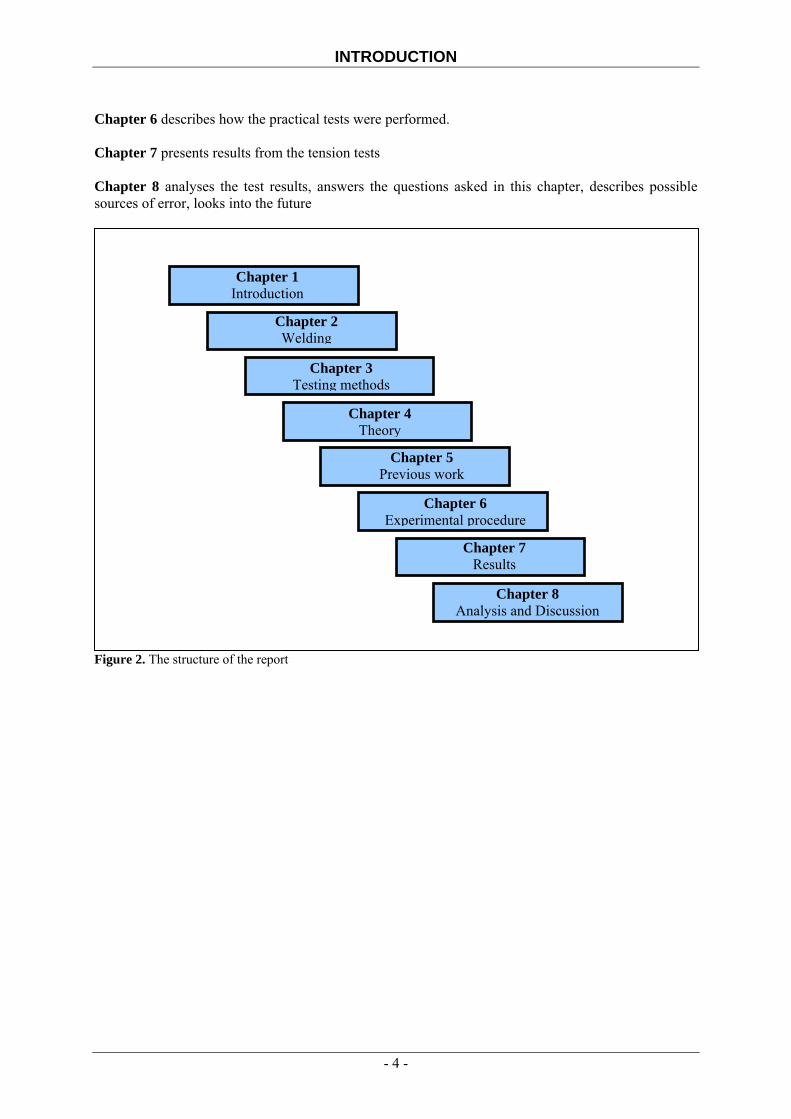
Chapter 6 describes how the practical tests were performed.

hapter 7 presents results from the tension tests

nswers the questions asked in this chapter, describes possible ources of error, looks into the future

igure 2. The structure of the report

C Chapter 8 analyses the test results, as

F

Chapter 1 Introduction

Chapter 2 Welding

Chapter 3 Testing methods

Chapter 4 Theory

Chapter 5 Previous work

Chapter 6 Experimental procedure

Chapter 7 Results

Chapter 8 Analysis and Discussion

- 4 -

WELDING

2 Welding

2.1 History

Welding is a fabrication process that joins materials, usually metals or plastics, by causing coalescence. This is often done by melting the work pieces and adding a filler material to form a pool of molten material that cools to become a joint, Weman (2002). This is in contrast with, for example soldering, where a material with a lower melting-point forms a bond between the work pieces without melting the base metal. People have been joining metals for several thousand years. The earliest examples of welding are from the Bronze and Iron Ages in Europe and the Middle East. During the medieval period advances were made in forge welding, in which blacksmiths pounded heated metal until bonding occurred. However when the Industrial Revolution, in the 19th century, took place welding was transformed. Invention of metal electrodes and the discovery of the electric arc changed the available techniques, according to Eriksson (1989). Most welding processes require high temperatures to unify the metals. Several different energy sources can be used, including a gas flame, an electric arc, a laser, an electron beam, friction and ultrasound, Svetskommissionen (2007). When modern welding was introduced, arc welding and its different welding methods became the largest and mostly used process. As the name indicates, the heat source is an electric arc between the base material and an electrode. The power supply can, according to Weman (2002) use either direct (DC) or alternating (AC) current and consumable or non-consumable electrodes are used. Electrical energy, transformed to heat, can generate an arc temperature up to 7000˚C. One of the main problems concerning welding is that heated metals react with the surrounding air. To protect the hot metal from the air is therefore important in welding. There are many different methods to protect the weld puddle from the air, ranging from flux covered electrodes (giving a protective slag) to inert or active shielding gases. Sometimes all the air is removed and welding is performed in vacuum. In 1906, the Swede Oscar Kjellberg obtained a patent for the covered electrode. He used welding to repair things but was not satisfied with his results. He covered his electrode with a material that melted and produced shielding slag. The result was extraordinary good and made the foundation for one of today’s largest welding companies, ESAB (Elektriska Svetsnings AB), Weman (2002). 2.2 Welding Processes

Below is a short description of some common welding processes, Bergh (1987) and Svetskommissionen (2007). 2.2.1 Manual Metal Arc welding (MMA) Welding with covered electrodes or MMA is also known as Shielded Metal Arc Welding (SMAW) or stick welding. The electrode is made up of a core of steel which is covered with a flux. Electric current strikes an arc between the base material and the consumable electrode rod. When liquefied metal drops from the electrode core are transported by the arc into the weld pool they are protected from the air by CO2 gas formed by substances in the flux. The slag floats to the top of the puddle where it protects the molten material during the hardening.

- 5 -

WELDING

Electrodes are divided into three different groups depending on the chemical composition of the slag; acid, basic and rutile. Acid electrodes give an even and shiny pass. The slag is easy to remove. The weld has a lower yielding point and tensile strength than rutile or basic electrodes but gives a larger possible elongation. This kind of electrode is very rare in Sweden today. Rutile electrodes are easy to weld with and to ignite. The risk of hydrogen cracks limits the usage to carbon steels with a yield strength less than 440 [MPa] or carbon-manganese steels. Basic electrodes give a high quality weld in terms of strength, ductility and safety against heat induced cracks. The slag is normally harder to remove. Basic electrodes are hydroscopic and must therefore be protected from moisture. In spite of the rather long weld times due to electrode changes and slag chipping, it is probably the most common welding process for construction steels. Equipment is relatively inexpensive and the method is well suited for both the workshop and field jobs. Manual metal arc welding can be used for plate thicknesses larger than 2 mm. 2.2.2 Submerged Arc Welding (SAW) SAW-welding is a highly productive, mechanized welding method that can be performed with one or several continuous electrodes. The arc(s) are burning under a layer of protective flux that melts close to the arc and produces slag on the weld. The non-molten excess flux can be recycled. The arc is not visible under the flux, hence the name. The method is suitable for plate thicknesses above 2 mm and is often used for long horizontal welds, like for example beams. 2.2.3 Gas Metal Arc Welding (GMAW) In this method an arc is maintained between a continuous wire-electrode and the work piece. The weld is protected from contamination by an inert or active gas. Since the electrode is fed continuously, welding speeds are greater for GMAW than for MMA. Outside welding should be avoided since the protection from the gas decreases even in light winds. Gas metal arc welding with solid electrode is applied with short circuited metal transfer, called short-arc GMAW or with small molten metal droplets, called spray-arc GMAW. The short-arc welding is performed with low current and voltage and the electrode wire is thin. As a result the heat input is reduced, making it possible to weld thinner material while decreasing the amount of distortion and residual stress in the weld area. The droplets form on the tip of the electrode, but instead of dropping into the weld pool they bridge the gap between the electrode and the weld pool as a result of the greater wire feed rate. This causes a short circuit and extinguishes the arc, but is quickly reignited after the surface tension of the pool pulls the molten metal bead off the electrode tip. This process is repeated about 100 times per second, making the arc appear constant to the human eye. Spray-arc was the first metal transfer method used in GMAW. In this variation, molten metal droplets are rapidly passed along the stable electric arc from the electrode to the work piece. High amounts of voltage and current are necessary together with a relatively thick electrode. This means that the process involves high heat input and a large weld area and heat affected zone. As a result it is generally used on work pieces of thicknesses above 4 mm.

- 6 -

WELDING

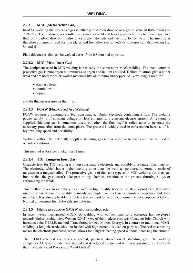
2.2.3.1 MAG (Metal Active Gas) In MAG-welding the protective gas is either pure carbon dioxide or a gas mixture of 80% argon and 20% CO2. The mixture gives a softer arc, smoother weld and fewer spatters but is a bit more expensive than only carbon dioxide. It also gives higher strength and ductility to the weld. The mixture is therefore commonly used for thin plates and low alloy steels. Today’s mixtures can also contain He, O2 and H2. Plate thicknesses that can be welded varies from 0,8 mm and upwards.

2.2.3.2 MIG (Metal Inert Gas) The equipment used in MIG-welding is basically the same as in MAG-welding. The most common protective gas is pure argon but mixtures of argon and helium are used. Helium mixtures give a hotter weld and are used for thick walled materials like aluminium and copper. MIG-welding is used for;

• stainless steels • a inium lum• copper

and for thicknesses greater than 1 mm.

2.2.3.3 FCAW (Flux-Cored Arc Welding) FCAW requires a continuously fed, consumable, tubular electrode containing a flux. The welding power supply is of constant voltage or, less commonly, a constant electric current. An externally supplied shielding gas is sometimes used, but often the flux itself is relied upon to generate the necessary protection from the atmosphere. The process is widely used in construction because of its high welding speed and portability. Welding without the externally supplied shielding gas is less sensitive to winds and can be used in outside conditions. This method is for steel thicker than 2 mm.

2.2.3.4 TIG (Tungsten Inert Gas) Characteristic for TIG-welding is a non-consumable electrode and possibly a separate filler material. The electrode, which has a higher melting point than the weld temperature, is normally made of tungsten or a tungsten alloy. The protective gas is of the same type as in MIG-welding. An inert gas implies that the gas doesn’t take part in any chemical reaction in the process (burning alloys or carbonizing the weld). This method gives an extremely clean weld of high quality because no slag is produced. It is often used in areas where the quality demands are high like nuclear-, chemistry-, airplane- and food industries. It is also applicable for metals that are hard to weld like titanium, Monel, copper-nickel etc. Normal dimensions for TIG-welds are 0,5-6 mm.

2.2.3.5 Highly productive GMAW with solid electrode In recent years mechanized MIG/MAG-welding with conventional solid electrode has developed towards higher productivity, Weman (2002). One of the predecessors was Canadian John Church who introduced the T.I.M.E.-method (Transferred Ionized Molten Energy). In contrast to traditional MAG-welding, a long electrode stick-out loaded with high current, is used on purpose. The resistive heating makes the electrode preheated, which allows for a higher feeding speed without increasing the current. The T.I.M.E.-method comprises a special, patented, 4-component shielding gas. The welding companies AGA and Linde have studied and developed the method with new gas mixtures. They call their methods Rapid Processing™ and Linfast®.

- 7 -

WELDING

With higher feeding speeds the productivity increases as well, sometimes up to 20 kg molten electrode per hour. The welding speed can be doubled, compared to conventional MAG-welding, with sustained weld deposit appearance and penetration profile. Different arc types are used. The most commonly used is a type of forced short arc which can be used on ordinary welding equipment. Yet another method to increase productivity and welding speeds is to use double electrodes. Both electrodes can be connected to the same source of current, this implies a more or less common arc (twin arc). If you instead have double sources of current, each connected to a separate electrode, it is referred to as tandem welding. The electrodes are still so close to each other that they weld in the same weld pool. The weld speeds can be at least doubled with double electrodes, in thin plates welding speeds can be even higher. 2.3 Hardening/Heat treatment

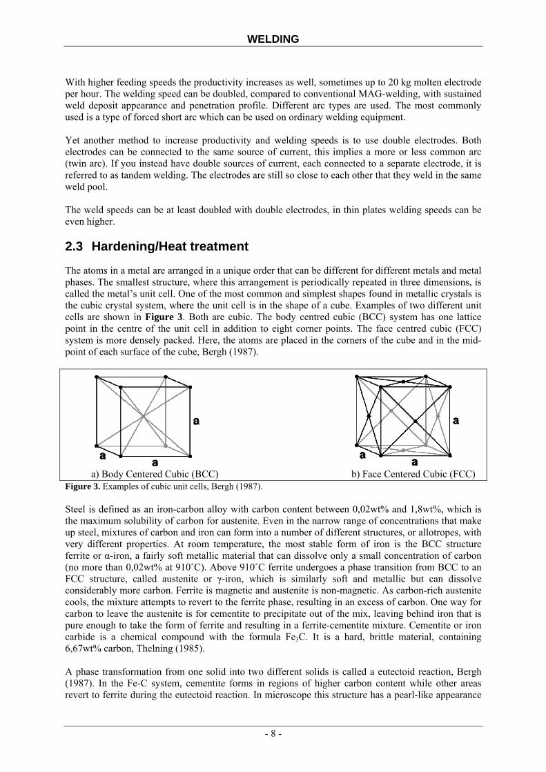
The atoms in a metal are arranged in a unique order that can be different for different metals and metal phases. The smallest structure, where this arrangement is periodically repeated in three dimensions, is called the metal’s unit cell. One of the most common and simplest shapes found in metallic crystals is the cubic crystal system, where the unit cell is in the shape of a cube. Examples of two different unit cells are shown in Figure 3. Both are cubic. The body centred cubic (BCC) system has one lattice point in the centre of the unit cell in addition to eight corner points. The face centred cubic (FCC) system is more densely packed. Here, the atoms are placed in the corners of the cube and in the mid-point of each surface of the cube, Bergh (1987).

a) Body Centered Cubic (BCC) b) Face Centered Cubic (FCC) Figure 3. Examples of cubic unit cells, Bergh (1987). Steel is defined as an iron-carbon alloy with carbon content between 0,02wt% and 1,8wt%, which is the maximum solubility of carbon for austenite. Even in the narrow range of concentrations that make up steel, mixtures of carbon and iron can form into a number of different structures, or allotropes, with very different properties. At room temperature, the most stable form of iron is the BCC structure ferrite or α-iron, a fairly soft metallic material that can dissolve only a small concentration of carbon (no more than 0,02wt% at 910˚C). Above 910˚C ferrite undergoes a phase transition from BCC to an FCC structure, called austenite or γ-iron, which is similarly soft and metallic but can dissolve considerably more carbon. Ferrite is magnetic and austenite is non-magnetic. As carbon-rich austenite cools, the mixture attempts to revert to the ferrite phase, resulting in an excess of carbon. One way for carbon to leave the austenite is for cementite to precipitate out of the mix, leaving behind iron that is pure enough to take the form of ferrite and resulting in a ferrite-cementite mixture. Cementite or iron carbide is a chemical compound with the formula Fe3C. It is a hard, brittle material, containing 6,67wt% carbon, Thelning (1985). A phase transformation from one solid into two different solids is called a eutectoid reaction, Bergh (1987). In the Fe-C system, cementite forms in regions of higher carbon content while other areas revert to ferrite during the eutectoid reaction. In microscope this structure has a pearl-like appearance

- 8 -

WELDING

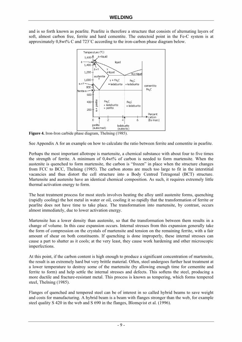
and is so forth known as pearlite. Pearlite is therefore a structure that consists of alternating layers of soft, almost carbon free, ferrite and hard cementite. The eutectoid point in the Fe-C system is at approximately 0,8wt% C and 723˚C according to the iron-carbon phase diagram below.

Figure 4. Iron-Iron carbide phase diagram, Thelning (1985).

See Appendix A for an example on how to calculate the ratio between ferrite and cementite in pearlite. Perhaps the most important allotrope is martensite, a chemical substance with about four to five times the strength of ferrite. A minimum of 0,4wt% of carbon is needed to form martensite. When the austenite is quenched to form martensite, the carbon is “frozen” in place when the structure changes from FCC to BCC, Thelning (1985). The carbon atoms are much too large to fit in the interstitial vacancies and thus distort the cell structure into a Body Centred Tetragonal (BCT) structure. Martensite and austenite have an identical chemical composition. As such, it requires extremely little thermal activation energy to form. The heat treatment process for most steels involves heating the alloy until austenite forms, quenching (rapidly cooling) the hot metal in water or oil, cooling it so rapidly that the transformation of ferrite or pearlite does not have time to take place. The transformation into martensite, by contrast, occurs almost immediately, due to lower activation energy. Martensite has a lower density than austenite, so that the transformation between them results in a change of volume. In this case expansion occurs. Internal stresses from this expansion generally take the form of compression on the crystals of martensite and tension on the remaining ferrite, with a fair amount of shear on both constituents. If quenching is done improperly, these internal stresses can cause a part to shatter as it cools; at the very least, they cause work hardening and other microscopic imperfections. At this point, if the carbon content is high enough to produce a significant concentration of martensite, the result is an extremely hard but very brittle material. Often, steel undergoes further heat treatment at a lower temperature to destroy some of the martensite (by allowing enough time for cementite and ferrite to form) and help settle the internal stresses and defects. This softens the steel, producing a more ductile and fracture-resistant metal. This process is known as tempering, which forms tempered steel, Thelning (1985). Flanges of quenched and tempered steel can be of interest in so called hybrid beams to save weight and costs for manufacturing. A hybrid beam is a beam with flanges stronger than the web, for example steel quality S 420 in the web and S 690 in the flanges, Blomqvist et al. (1996).

- 9 -

WELDING

2.4 Weld geometry

The weld geometry is chosen considering the welding process and thickness of the work piece. It is important to choose a geometry which satisfies the required demands on strength and quality without an unnecessarily large weld volume. The welding costs increases with the volume and an increase of the heat input can cause fracture resistance- and deformation problems Weman (2002).

Figure 5. Terminology for different parts of the joint, Weman (2002).

Groove angle

Bevel angle

Root opening Root

Root face and Groove face

Welds can be shaped geometrically in many different ways. The five basic types of weld joints are (Figure 6); the butt joint, the lap-joint, the corner joint, the edge joint and the T-joint, Eriksson (1989). Other variations exist as well – for example double-V preparation joints are characterized by the two pieces of material each tapering to a single centre point at one-half of their height. Single-U and double-U preparation joints are also fairly common. Lap joints are often more than two pieces thick, depending on the process used and the thickness of the material, many pieces can be welded together in a lap-joint geometry.

Figure 6. Common welding geometries, Weman (2002).

1a: Square butt joint

1b: Double-V preparation butt joint

1c: Single-U preparation butt joint

2: Lap-joint

3: Full open corner joint

4: Flanged edge joint

5: T-joint

- 10 -

WELDING

Often particular joint designs are used, almost exclusively, by certain welding processes. For example, resistance spot welding, laser beam welding, and electron beam welding are most frequently performed on lap-joints. However, some welding methods, like shielded metal arc welding, are extremely versatile and can weld virtually any type of joint, Weman (2002). 2.5 Heat Affected Zones

After welding, a number of distinct regions can be identified in the weld area. The weld itself is called the fusion zone – more specifically this is where the filler material has blended together with the base metal to a hardened weld puddle, Weman (2002). The properties of the fusion zone depend primarily on the filler material used and its compatibility with the base materials. It is surrounded by the heat-affected zone, the area that had its microstructure and properties altered by the weld. These properties depend on the base material’s behaviour when subjected to heat. The metal in this area is often weaker than both the base material and the fusion zone and is also where residual stresses are found. In the heat affected zone of a welded joint the peak temperature has been high enough to produce solid-state microstructural changes, but too low to cause melting. The size, microstructural characteristics and mechanical properties of the HAZ are a function of the type of base metal being welded, chemical composition of the base metal, heat input and the part thickness. The transduced zone in Figure 7 is commonly divided into; a normalized zone and an over-heated zone, Weman (2002).

Figure 7. Nomenclature for boundaries and different zones according to the Swedish welding commission, Weman (2002).

Initial joint surface

Non-affected base material

Penetration zone

Transduced zone

Structurally changed zone

Melting boundary

Transmission boundary

Boundary for structural changes

Weld (fusion zone) Weld affected base material

Weld-affected area (HAZ)

Regions that are expected in single- and multi pass HAZ are described in the next section. 2.5.1 Single pass welds The heat affected zone of a single bead is divided into four major zones, each with its own properties, Figure 8. Region Approximate peak temperature Coarse-grained HAZ (CGHAZ) 1100˚C – melting point Fine-grained HAZ (FGHAZ) Ac3

* - 1100˚C Intercritical HAZ (ICHAZ) Ac1

† – Ac3

* The temperature at which austenitic transformation is completed during the heating process † The temperature at which austenitic transformation commences during the heating process

- 11 -

WELDING

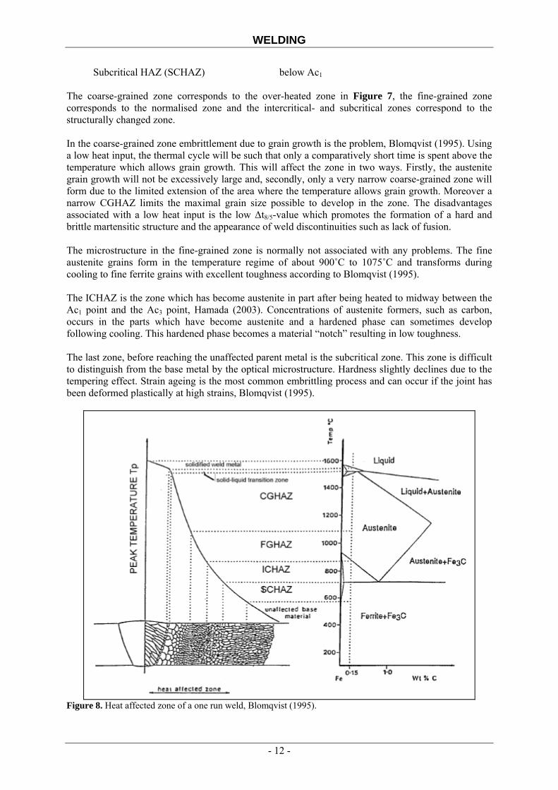
Subcritical HAZ (SCHAZ) below Ac1 The coarse-grained zone corresponds to the over-heated zone in Figure 7, the fine-grained zone corresponds to the normalised zone and the intercritical- and subcritical zones correspond to the structurally changed zone. In the coarse-grained zone embrittlement due to grain growth is the problem, Blomqvist (1995). Using a low heat input, the thermal cycle will be such that only a comparatively short time is spent above the temperature which allows grain growth. This will affect the zone in two ways. Firstly, the austenite grain growth will not be excessively large and, secondly, only a very narrow coarse-grained zone will form due to the limited extension of the area where the temperature allows grain growth. Moreover a narrow CGHAZ limits the maximal grain size possible to develop in the zone. The disadvantages associated with a low heat input is the low Δt8/5-value which promotes the formation of a hard and brittle martensitic structure and the appearance of weld discontinuities such as lack of fusion. The microstructure in the fine-grained zone is normally not associated with any problems. The fine austenite grains form in the temperature regime of about 900˚C to 1075˚C and transforms during cooling to fine ferrite grains with excellent toughness according to Blomqvist (1995). The ICHAZ is the zone which has become austenite in part after being heated to midway between the Ac1 point and the Ac3 point, Hamada (2003). Concentrations of austenite formers, such as carbon, occurs in the parts which have become austenite and a hardened phase can sometimes develop following cooling. This hardened phase becomes a material “notch” resulting in low toughness. The last zone, before reaching the unaffected parent metal is the subcritical zone. This zone is difficult to distinguish from the base metal by the optical microstructure. Hardness slightly declines due to the tempering effect. Strain ageing is the most common embrittling process and can occur if the joint has been deformed plastically at high strains, Blomqvist (1995).

Figure 8. Heat affected zone of a one run weld, Blomqvist (1995).

- 12 -

WELDING

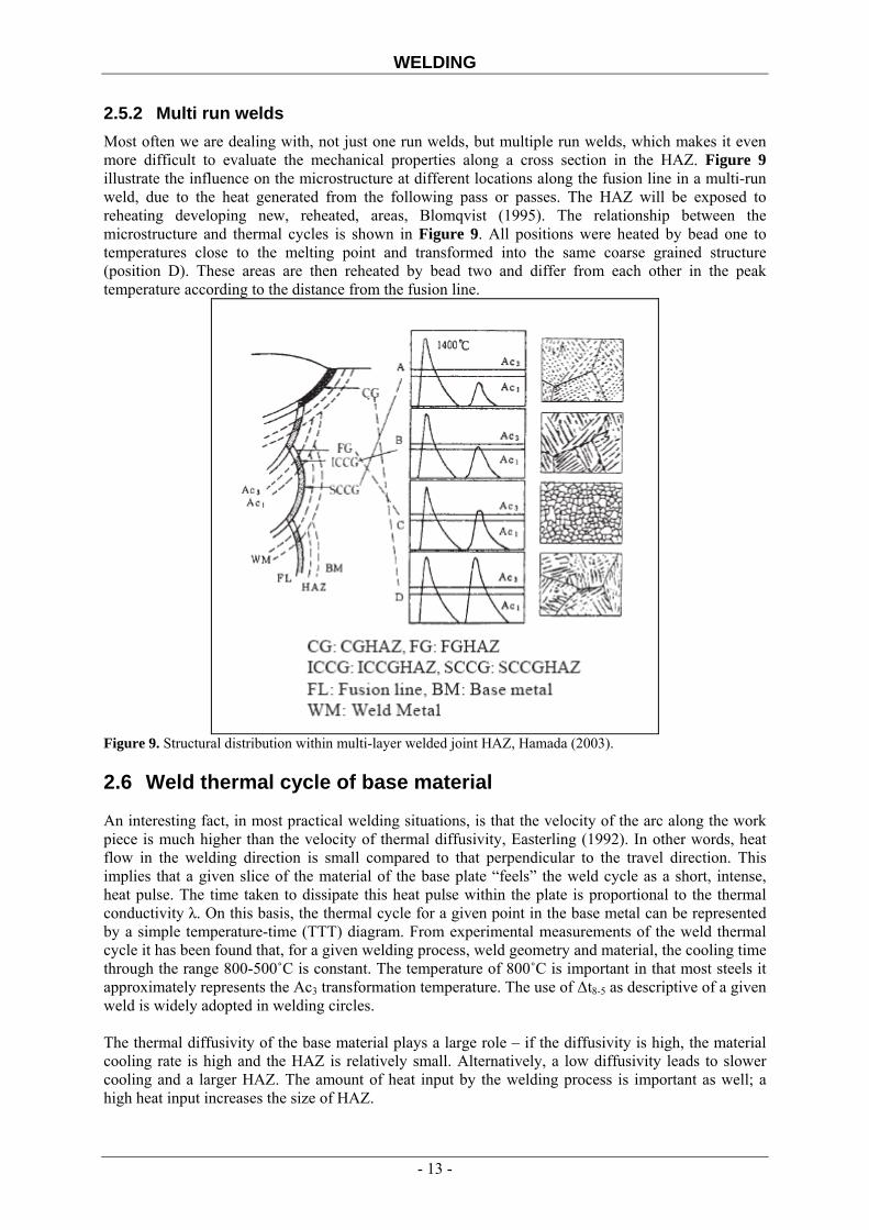
2.5.2 Multi run welds Most often we are dealing with, not just one run welds, but multiple run welds, which makes it even more difficult to evaluate the mechanical properties along a cross section in the HAZ. Figure 9 illustrate the influence on the microstructure at different locations along the fusion line in a multi-run weld, due to the heat generated from the following pass or passes. The HAZ will be exposed to reheating developing new, reheated, areas, Blomqvist (1995). The relationship between the microstructure and thermal cycles is shown in Figure 9. All positions were heated by bead one to temperatures close to the melting point and transformed into the same coarse grained structure (position D). These areas are then reheated by bead two and differ from each other in the peak temperature according to the distance from the fusion line.

Figure 9. Structural distribution within multi-layer welded joint HAZ, Hamada (2003). 2.6 Weld thermal cycle of base material

An interesting fact, in most practical welding situations, is that the velocity of the arc along the work piece is much higher than the velocity of thermal diffusivity, Easterling (1992). In other words, heat flow in the welding direction is small compared to that perpendicular to the travel direction. This implies that a given slice of the material of the base plate “feels” the weld cycle as a short, intense, heat pulse. The time taken to dissipate this heat pulse within the plate is proportional to the thermal conductivity λ. On this basis, the thermal cycle for a given point in the base metal can be represented by a simple temperature-time (TTT) diagram. From experimental measurements of the weld thermal cycle it has been found that, for a given welding process, weld geometry and material, the cooling time through the range 800-500˚C is constant. The temperature of 800˚C is important in that most steels it approximately represents the Ac3 transformation temperature. The use of Δt8-5 as descriptive of a given weld is widely adopted in welding circles. The thermal diffusivity of the base material plays a large role – if the diffusivity is high, the material cooling rate is high and the HAZ is relatively small. Alternatively, a low diffusivity leads to slower cooling and a larger HAZ. The amount of heat input by the welding process is important as well; a high heat input increases the size of HAZ.

- 13 -

WELDING

For thick plates, Δt8-5 is approximately proportional to the heat input Q. Qkt 58 ⋅≈Δ − (2.1) where k is in the range of 4-5 seconds per kJ/mm for conventional structural steels, Qiu et al. (2001). 2.7 Weldability

Most often, the quality of a weld is judged by its strength and the strength of the material around it. Many factors influence this, including the welding method, the amount and concentration of heat input, the base material, the filler material, the flux, the design of the joint and interactions between all these factors, Weman (2002). To test the quality of a weld either destructive or non-destructive methods are used to verify that welds are defect-free, have acceptable levels of residual stresses and distortion and have acceptable heat-affected zone (HAZ) properties. Not all metals are suitable for welding and all filler metals do not work well with acceptable base materials. The weldability of steel is inversely proportional to a property known as the hardenability of the steel, which measures the ease of forming martensite during heat treatment. The hardenability of the steel depends on its chemical composition, with higher concentrations of carbon and other alloying elements such as manganese, chromium, silicon, molybdenum, vanadium, copper and nickel tend to increase the hardness and decrease the weldability of the material, Easterling (1992). Each of these substances influences the hardness and weldability to different magnitudes. This makes a method of comparison necessary to judge the difference in hardness between two alloys made of different alloying elements. A measure known as the equivalent carbon content is used to compare the relative weldabilities of different alloys by comparing their properties to plain carbon steel.

15

NiCu5

VMoCr6

MnCEc+

+++

++= (2.2)

A steel is considered fully weldable if Ec is below 0,41. For higher Ec levels the steel is denoted limited weldable, which in general means that welding should be performed with a pre-heated work-piece to reduce the cooling rate Weman (2002). Stainless steels, because of their high chromium content, tend to behave differently with respect to weldability than other steels. Austenitic grades of stainless steel tend to be the most weldable, but they are especially sensitive to distortion due to their high coefficient of thermal expansion. Hot cracking is possible if the amount of ferrite in the weld is not controlled, to alleviate this problem an electrode is used that deposits a weld metal containing a small amount of ferrite. Other types of stainless steels, such as ferritic and martensitic stainless steels, are not as easily welded and must often be preheated and welded with special electrodes Weman (2002). 2.8 Cracking

Welding methods that involve melting metal at the site of the joint are prone to shrinkage as the heated metal cools. Shrinkage, in turn, can introduce residual stresses and both longitudinal and rotational distortion, Eriksson (1989). Distortion can pose a major problem since the final product is not the desired shape. To alleviate rotational distortion, the work pieces can be offset, so that the welding results in a correctly shaped piece. Other methods of limiting distortion, such as clamping the work pieces in place, cause the build-up of residual stress in the heat-affected zone of the base material. These stresses can reduce the strength of the base material and can lead to failure through cold cracking.

- 14 -

WELDING

Another name for cold cracking is hydrogen-induced cracking or delayed cracking. The common source of hydrogen is from moisture. Grease, oxides and other contaminants are also potential sources of hydrogen, Coe (1973). Hydrogen from these sources can be introduced into the weld region through the welding electrode, shielding materials, the base metal surface and the atmosphere. The cracking occurs in the heat-affected zone (HAZ) of the base material and in the fusion zone (FZ). While the reasons for cracking are the same, controlling the factors that cause cracking can be different for the HAZ and FZ. For the HAZ, control of cracking comes from the steel making processes, which incorporate means to avoid susceptible microstructures and eliminate sources of hydrogen in the base metal. For the FZ, control of susceptibility to hydrogen-induced cracking is achieved by adding alloying elements in the consumables and using proper welding techniques, including preheat and heat input. The most common and effective method of eliminating hydrogen-induced cracking is by specifying minimum preheat and interpass temperatures for welding. In general, a higher preheat temperature reduces the chance for formation of brittle microstructures and gives more time for the hydrogen to diffuse from the weld, Coe (1973). A ground rule when welding quenched and tempered steel is to always use consumables with low hydrogen content, Blomqvist et al. (1996). The other type of cracking, hot cracking or solidification cracking, can occur in all metals and happens in the fusion zone of a weld. To reduce the probability of this type of cracking, excess material restraint should be avoided and a proper filler material should be utilized, Eriksson (1989). 2.9 Electrode Matching

A mismatch in a weld is regarded as a difference in the strength levels between the weld metal, base metal and the heat-affected zone, Blomqvist et al. (1996). The mismatch factor M is identified as the ratio of the yield strength of the weld metal to the yield strength of the base metal.

bmy

wmy

ff

M = (2.3)

For M > 1 the weld is over-matched otherwise it is under-matched. It has been shown that the volume of the weld metal (the width of the weld in relation to the plate thickness), using an undermatching electrode, can be considered to be a “soft zone” which is crucial for the strength of the joint. By minimizing the volume of the weld metal it has shown to be possible, despite an undermatching weld, to achieve a joint that matches the base metal in strength. This is possible due to the tri-axial stress distribution that occurs when loading the weld. This triaxiality in a surrounding material of higher strength increases the strength of the joint, Blomqvist et al. (1996). To combine over- and undermatching weld metals is common today, Blomqvist et al. (1996). This means that the root pass is undermatching and the filler passes are welded with overmatching consumables. That the weld metal contains a small amount of soft additive does not reduce the strength of the joint significantly. For EHS (Extra High Strength) steels, with yield strengths of approximately 500 MPa, there is a large number of electrodes to utilize. The values presented by the electrode manufactures are often results from standardized conditions. In practice the weld metal’s strength and ductility is not only dependant on its chemical composition but also on the welding procedure i.e. the choice of heat input, electrode diameter, number of passes, the weld geometry and so on, Blomqvist et al. (1996).

- 15 -

WELDING

An important aspect, when welding high strength steels, is to choose a consumable with the lowest possible strength. A consumable of lower strength than the base material simplifies the welding and makes it easier to attain a crack-free joint, Blomqvist et al. (1996). Welding with undermatching electrodes normally results in a weld with high ductility. According to Blomqvist et al. (1996), advantages of welding with undermatching electrodes are;

• a reduction of residual stresses in the joint • a reduction of the influence of welding discontinuities, related to manufacturing • better ductility • less need for pre-heating when welding thicker plates

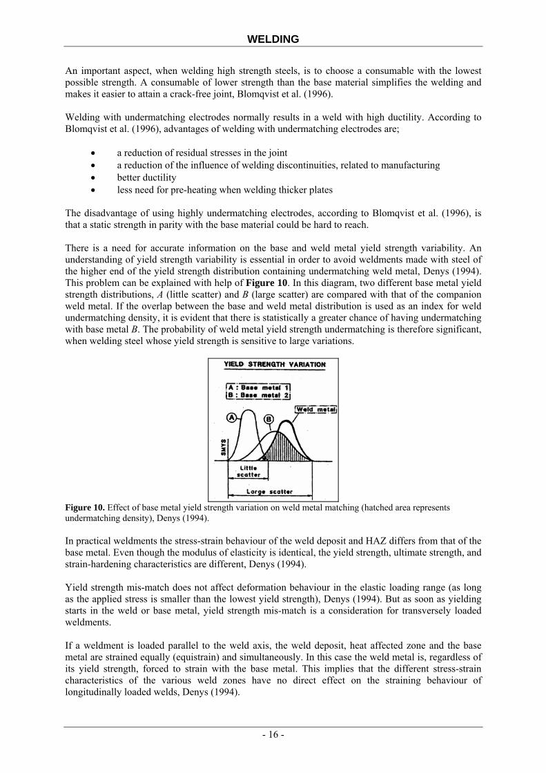
The disadvantage of using highly undermatching electrodes, according to Blomqvist et al. (1996), is that a static strength in parity with the base material could be hard to reach. There is a need for accurate information on the base and weld metal yield strength variability. An understanding of yield strength variability is essential in order to avoid weldments made with steel of the higher end of the yield strength distribution containing undermatching weld metal, Denys (1994). This problem can be explained with help of Figure 10. In this diagram, two different base metal yield strength distributions, A (little scatter) and B (large scatter) are compared with that of the companion weld metal. If the overlap between the base and weld metal distribution is used as an index for weld undermatching density, it is evident that there is statistically a greater chance of having undermatching with base metal B. The probability of weld metal yield strength undermatching is therefore significant, when welding steel whose yield strength is sensitive to large variations.

Figure 10. Effect of base metal yield strength variation on weld metal matching (hatched area represents undermatching density), Denys (1994). In practical weldments the stress-strain behaviour of the weld deposit and HAZ differs from that of the base metal. Even though the modulus of elasticity is identical, the yield strength, ultimate strength, and strain-hardening characteristics are different, Denys (1994). Yield strength mis-match does not affect deformation behaviour in the elastic loading range (as long as the applied stress is smaller than the lowest yield strength), Denys (1994). But as soon as yielding starts in the weld or base metal, yield strength mis-match is a consideration for transversely loaded weldments. If a weldment is loaded parallel to the weld axis, the weld deposit, heat affected zone and the base metal are strained equally (equistrain) and simultaneously. In this case the weld metal is, regardless of its yield strength, forced to strain with the base metal. This implies that the different stress-strain characteristics of the various weld zones have no direct effect on the straining behaviour of longitudinally loaded welds, Denys (1994).

- 16 -

WELDING

The load-elongation behaviour of a transversely loaded weldment at the onset of yielding is controlled by the weld metal with the lowest yield strength, i.e. either the base- or weld metal yield strength

etermines the onset of plastic straining, Denys (1994). d

Figure 11. Effect of weld metal overmatching (A) and weld metal undermatching (B) on stress and strain

istribution in a longitudinally (a) and transversally (b) loaded weldment, Denys (1994).

base metal is required to initiate plastic deformation in an overmatching weld metal, enys (1994).

n ardening capacity or the yield- to tensile strength ratios of the base and weld metals, Denys (1994).

and weld metal ultimate tensile strength (TW), can be ombined in six ways (Table 1), Denys (1994).

tal – base metal comMBINATION SEQU ENA

d When the weld metal yield strength is lower than that of the base metal, the applied strain is concentrated as plastic strain in the weld metal and HAZ regions. If the weld metal yield strength exceeds the base metal yield strength, plastic straining occurs in the base metal. For base metal yielding to occur, in undermatching weldments, the weld metal must strain harden. Equally, strain-hardening of theD The knowledge of the base- and weld metal yield strengths alone is not sufficient to determine the yielding pattern and the plastic straining capability of a weldment. It also depends on the straih Several different base- and weld metal combinations are used to fabricate weldments. From a theoretical point of view, the four variables; base metal yield strength (YB), weld metal yield strength (YW), base metal ultimate tensile strength (TB) c Table 1. Weld me binations CO ENCE OF PHENOM TYPE A YW<TW<YB<TB Undermatching B YW<YB<TW<TB Undermatching C YW<YB<TB<TW Undermatching D YB<TB<YW<TW Overmatching E YB<YW<TB<TW Overmatching F YB<YW<TW<TB Overmatching Figure 12 summarizes the deformation behaviour at failure. The hatched areas represent plastically strained region(s) at failure and the dashed lines indicate the location of failure. Combination A, B and C produce undermatching weldments, whereas combinations D, E and F contain a weld deposit which is overmatching in yield strength. Figure 12 illustrates that five of the six combinations fail only after base metal yielding, Denys (1994).

- 17 -

WELDING

Figure 12. Schematic diagram showing base metal – weld metal combinations with indication of the corresponding yield pattern and failure location, Denys (1994). Figure 12 verifies that yield strength variability makes it possible to obtain different weld combinations for a steel delivered to a certain minimum specified yield strength, Denys (1994). Other important features are:

• base metal yielding is not excluded for yield strength undermatching weld metal (combinations B and C);

• base metal failure can occur with yield strength undermatching weld metal (combination C); • base metal failure can occur with an elastically stressed overmatching weld metal

(combination D); • weld metal failure is not excluded with yield strength overmatching weld metal

(combination F). The failure – deformation behaviour depends also on the base- and weld metal strain hardening capability (Figure 13). For example, for undermatching weld metals with a very low strain hardening capacity or very high YS/TS-ratio, the probability of base metal plastic straining is low or even excluded, Denys (1994). Conversely, weld metals having high strain hardening capacity foster base metal plastic straining. Figure 13 illustrates, moreover, that with decreasing strain hardening capacity more weld metal straining (ew) is required to reach the base metal yield strength.

Figure 13. Representation of the effect of weld metal strain hardening on weld strain, ew, for an undermatching weld metal, Denys (1994).

- 18 -

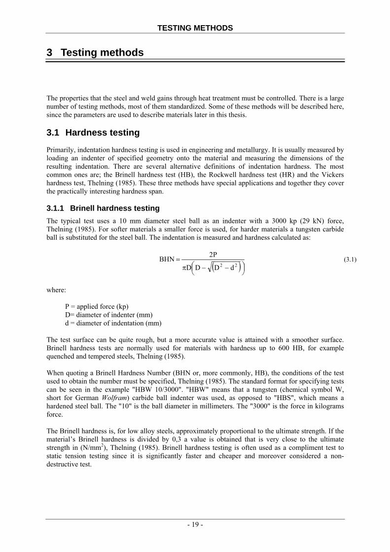
TESTING METHODS

3 Testing methods

The properties that the steel and weld gains through heat treatment must be controlled. There is a large number of testing methods, most of them standardized. Some of these methods will be described here, since the parameters are used to describe materials later in this thesis. 3.1 Hardness testing

Primarily, indentation hardness testing is used in engineering and metallurgy. It is usually measured by loading an indenter of specified geometry onto the material and measuring the dimensions of the resulting indentation. There are several alternative definitions of indentation hardness. The most common ones are; the Brinell hardness test (HB), the Rockwell hardness test (HR) and the Vickers hardness test, Thelning (1985). These three methods have special applications and together they cover the practically interesting hardness span. 3.1.1 Brinell hardness testing The typical test uses a 10 mm diameter steel ball as an indenter with a 3000 kp (29 kN) force, Thelning (1985). For softer materials a smaller force is used, for harder materials a tungsten carbide ball is substituted for the steel ball. The indentation is measured and hardness calculated as:

( )⎟

⎠⎞⎜

⎝⎛ −−π

=22 dDDD

P2BHN (3.1)

where:

P = applied force (kp) D= diameter of indenter (mm) d = diameter of indentation (mm)

The test surface can be quite rough, but a more accurate value is attained with a smoother surface. Brinell hardness tests are normally used for materials with hardness up to 600 HB, for example quenched and tempered steels, Thelning (1985). When quoting a Brinell Hardness Number (BHN or, more commonly, HB), the conditions of the test used to obtain the number must be specified, Thelning (1985). The standard format for specifying tests can be seen in the example "HBW 10/3000". "HBW" means that a tungsten (chemical symbol W, short for German Wolfram) carbide ball indenter was used, as opposed to "HBS", which means a hardened steel ball. The "10" is the ball diameter in millimeters. The "3000" is the force in kilograms force. The Brinell hardness is, for low alloy steels, approximately proportional to the ultimate strength. If the material’s Brinell hardness is divided by 0,3 a value is obtained that is very close to the ultimate strength in (N/mm2), Thelning (1985). Brinell hardness testing is often used as a compliment test to static tension testing since it is significantly faster and cheaper and moreover considered a non-destructive test.

- 19 -

TESTING METHODS

3.1.2 Vickers hardness test The Vickers hardness test is an alternative method to measure the hardness of materials. The reasons to why it is easier to use than other hardness tests is that calculations are not dependent on the size of the indenter and also that the indenter can be used for all materials irrespective of hardness, Thelning (1985). The Vickers hardness test uses a diamond, with the shape of a square-based pyramid with an angle of 136˚ between opposite faces, as an indenter, Thelning (1985). Loads of various magnitudes can be applied, depending on the hardness of the material to be measured. The diagonals of the quadratic indent are measured and the Vickers Pyramid Number (HV) can be found in tables.

2dP854,1

APHV ⋅≈= (3.2)

where P = applied force (kp) d = average length of the diagonal left by the indenter (mm) Vickers hardness numbers are reported as 850HV10, where 850 is the hardness number, HV gives the hardness scale (Vickers) and 10 indicates the load used in kp, Thelning (1985). 3.1.3 Rockwell hardness test There are several alternative Rockwell scales; the most commonly used being the “B” and “C” scales. Both express the hardness as an arbitrary dimensionless number. Of the hardness testing methods based on measuring the depth or width of the indentation, Rockwell is the fastest method thanks to its ability to display hardness values directly with relatively high accuracy, Thelning (1985). In all scales the sample is loaded with a minor load (F0) followed by a major load (F1) applied during 5-10 s. After unburdening to the minor load the hardness can be noted directly from a dial. The hardness is a function of the increase in penetration achieved by loading and unloading F1, Thelning (1985). 3.2 Tensile testing

The tensile test is one of the older material-testing methods and has been used, since the beginning of industrialism (1830’s), to determine the stress a material can be exposed to during a static load, Eriksson (2005). Normally, in tensile tests, a smooth cylindrical (circular cross-sectional area) or parallelepiped (rectangular cross-sectional area) test specimen is used. The specimen is often equipped with grip areas to ease the mounting into the machine and to avoid having fracture in the area being gripped, Eriksson (2005). The modern testing equipment is an electronically controlled, hydraulic/mechanic machine, originally it was completely mechanical. The specimen is forced to deform, in terms of elongation, until fracture occurs. The loading-rate is low and the time to perform a test is in the vicinity of a minute, Eriksson (2005). During the course of the test, the load and elongation of the test specimen are recorded. The stress, σ, in the specimen is:

- 20 -

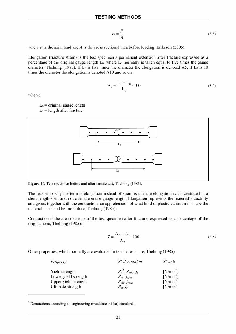
TESTING METHODS

AF

=σ (3.3)

where F is the axial load and A is the cross sectional area before loading, Eriksson (2005). Elongation (fracture strain) is the test specimen’s permanent extension after fracture expressed as a percentage of the original gauge length L0, where L0 normally is taken equal to five times the gauge diameter, Thelning (1985). If L0 is five times the diameter the elongation is denoted A5, if L0 is 10 times the diameter the elongation is denoted A10 and so on.

100L

LLA

0

01i ⋅

−= (3.4)

where: L0 = original gauge length L1 = length after fracture

Figure 14. Test specimen before and after tensile test, Thelning (1985).

A0

L0

L1

A1

The reason to why the term is elongation instead of strain is that the elongation is concentrated in a short length-span and not over the entire gauge length. Elongation represents the material’s ductility and gives, together with the contraction, an apprehension of what kind of plastic variation in shape the material can stand before failure, Thelning (1985). Contraction is the area decrease of the test specimen after fracture, expressed as a percentage of the original area, Thelning (1985):

100A

AAZ

0

10 ⋅−

= (3.5)

Other properties, which normally are evaluated in tensile tests, are, Thelning (1985): Property SI-denotation SI-unit Yield strength Re

3, Rp0,2 y, f [N/mm ] 2

Lower yield strength ReL, fy,inf [N/mm2] Upper yield strength ReH, fy,sup [N/mm2] Ultimate strength Rm, fu [N/mm2]

3 Denotations according to engineering (maskintekniska) standards

- 21 -

TESTING METHODS

The yield strength is the largest stress for which deformations are elastic. An irregular transition area appears in mild steels of medium strength. In this area, both an upper- and lower yield strength is determined. The yield strength for high-strength steels, which lacks a well defined yield plateau, is in practice defined as the stress that corresponds to a small permanent deformation, 0,2% - called the 0,2 offset yield strength, Eriksson (2005). The ultimate strength is determined from the σ-ε-diagram, as the maximum point of the curve, Eriksson (2005). 3.3 Fracture toughness testing

3.3.1 Background During pre-World War II, welding rivalled riveting as a method of joining steel. There were, however, a large number of brittle failures in foremost bridges and ships during this time. These break-downs initiated the development of modern construction steels with high strength, ductility and weldability, Eriksson (2005). The most well known failures include the Hasselt bridge in Belgium (1938) and the transport ship Schenectady in Portland (1942). During WW II, USA built a large number of, so called Liberty ships, in a short time. These ships were designed to transport military materiel to Europe for the invasion of Normandy. Out of approximately 5000 ships, 1000 were severely damaged by brittle fracture and over 200 were more or less split in halves, Eriksson (2005). Extensive investigations revealed that the fracture started in a crack-like, initial, defect often close to sharp corners or welded joints. Steels that were considered ductile to very low temperatures according to conventional tensile tests, could actually fail at room temperature due to defects. New testing methods, which would imitate critical factors for brittle failure, were developed. A common element of the different test specimens was that all had an initial defect, Eriksson (2005). The resistance to fracture of a material is known as its fracture toughness. Fracture toughness generally depends on temperature, environment, loading rate, the composition of the material and its microstructure, together with geometric effects (constraint). These factors are of particular importance for welded joints where the metallurgical and geometric effects are complex, TWI (2007). Fracture toughness is a critical input parameter for fracture-mechanics based fitness-for-service assessments. Although fracture toughness can sometimes be obtained from the literature or materials properties databases, it is preferable to determine this by experiment for the particular material and joint being assessed, TWI (2007). Various measures of “toughness” exist, including the widely used but qualitative Charpy impact test. Although it is possible to correlate Charpy energy with fracture toughness, a large degree of uncertainty is associated with correlations because they are empirical. It is preferable to determine fracture toughness in a rigorous fashion, in terms of K (stress intensity factor), CTOD (crack tip opening displacement) or J (the J integral). Standards exist for performing fracture mechanics tests, with the most common specimen configuration shown in Figure 15 (the single edged notch bend, SENB, specimen). A sharp fatigue notch is inserted in the specimen, which is loaded to failure. The crack driving force is calculated for the failure condition, giving the fracture toughness, TWI (2007).

- 22 -

TESTING METHODS

Figure 15. Fracture mechanics testing, TWI (2007). 3.3.2 Test specimens The most widely used fracture toughness test configurations are the single edge notch bend (SENB or three point bend) and the compact (CT) specimens, as shown in Figure 16. The compact specimen has the advantage that it requires less material, but is more expensive to machine and more complex to test compared with the SENB specimen. Also special requirements are needed for temperature control (e.g. use of an environmental chamber). SENB specimens are typically immersed in a bath for low temperature tests. Although the compact specimen is loaded in tension, the crack tip conditions are predominantly bending (high constraint). If limited material is available, it is possible to fabricate SENB specimens by welding extension pieces (for the loading arms) to the material sample. Electron beam welding is typically used, because the weld is narrow and causes little distortion, TWI (2007).

Figure 16. Examples of common fracture toughness test specimen types, TWI (2007). Other specimen configurations include centre-cracked tension (CCT) panels, single edge notch tension (SENT) specimens and shallow-crack tests. These specialized tests are associated with lower levels of constraint and can be more structurally representative than standard SENB or CT specimens, TWI (2007). The position and orientation of the specimen is important. In particular, the location and orientation of the notch is critical, especially for welded joints. Typically, the notch (fatigue pre-crack) is positioned such that a chosen microstructure is sampled. The orientation of the notch is defined with respect to either the weld axis for welded joints, or the rolling direction or forging axis for other components, TWI (2007).

- 23 -

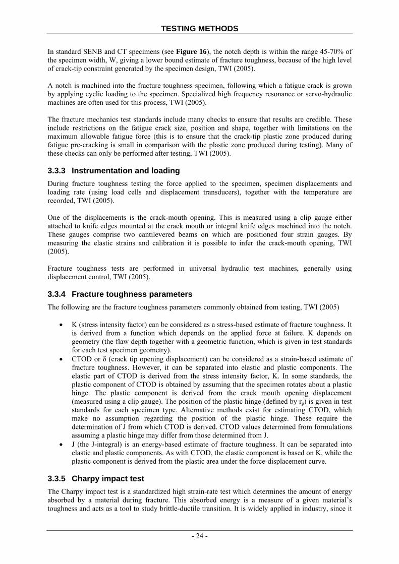
TESTING METHODS

In standard SENB and CT specimens (see Figure 16), the notch depth is within the range 45-70% of the specimen width, W, giving a lower bound estimate of fracture toughness, because of the high level of crack-tip constraint generated by the specimen design, TWI (2005). A notch is machined into the fracture toughness specimen, following which a fatigue crack is grown by applying cyclic loading to the specimen. Specialized high frequency resonance or servo-hydraulic machines are often used for this process, TWI (2005). The fracture mechanics test standards include many checks to ensure that results are credible. These include restrictions on the fatigue crack size, position and shape, together with limitations on the maximum allowable fatigue force (this is to ensure that the crack-tip plastic zone produced during fatigue pre-cracking is small in comparison with the plastic zone produced during testing). Many of these checks can only be performed after testing, TWI (2005). 3.3.3 Instrumentation and loading During fracture toughness testing the force applied to the specimen, specimen displacements and loading rate (using load cells and displacement transducers), together with the temperature are recorded, TWI (2005). One of the displacements is the crack-mouth opening. This is measured using a clip gauge either attached to knife edges mounted at the crack mouth or integral knife edges machined into the notch. These gauges comprise two cantilevered beams on which are positioned four strain gauges. By measuring the elastic strains and calibration it is possible to infer the crack-mouth opening, TWI (2005). Fracture toughness tests are performed in universal hydraulic test machines, generally using displacement control, TWI (2005). 3.3.4 Fracture toughness parameters The following are the fracture toughness parameters commonly obtained from testing, TWI (2005)

• K (stress intensity factor) can be considered as a stress-based estimate of fracture toughness. It is derived from a function which depends on the applied force at failure. K depends on geometry (the flaw depth together with a geometric function, which is given in test standards for each test specimen geometry).

• CTOD or δ (crack tip opening displacement) can be considered as a strain-based estimate of fracture toughness. However, it can be separated into elastic and plastic components. The elastic part of CTOD is derived from the stress intensity factor, K. In some standards, the plastic component of CTOD is obtained by assuming that the specimen rotates about a plastic hinge. The plastic component is derived from the crack mouth opening displacement (measured using a clip gauge). The position of the plastic hinge (defined by rp) is given in test standards for each specimen type. Alternative methods exist for estimating CTOD, which make no assumption regarding the position of the plastic hinge. These require the determination of J from which CTOD is derived. CTOD values determined from formulations assuming a plastic hinge may differ from those determined from J.

• J (the J-integral) is an energy-based estimate of fracture toughness. It can be separated into elastic and plastic components. As with CTOD, the elastic component is based on K, while the plastic component is derived from the plastic area under the force-displacement curve.

3.3.5 Charpy impact test The Charpy impact test is a standardized high strain-rate test which determines the amount of energy absorbed by a material during fracture. This absorbed energy is a measure of a given material’s toughness and acts as a tool to study brittle-ductile transition. It is widely applied in industry, since it

- 24 -

TESTING METHODS

is easy to prepare and conduct and results can be obtained quickly and cheaply. But a major disadvantage is that all results are only comparative, TWI (2005). It was developed by the French scientist Georges Charpy, TWI (2005). The qualitative results of the fracture may be used to determine the toughness of the material. Also, this test may be done with the material at various temperatures to determine the brittle-ductile transition temperature, TWI (2005). 3.3.6 Definition The apparatus consists of a pendulum hammer swinging at a notched sample of material (Figure 17). The energy transferred to the material can be inferred by comparing the difference in the height of the hammer before and after fracture. If a typical 325-J machine was used, the extreme final positions of the pendulum would be either at the same height of the pendulum before it was released (indicating no energy loss in breaking the sample), or at the bottom of its travel (indicating that the specimen absorbed the full 325 joules of energy). The dial provides a direct readout of the energy absorbed by the sample, Eriksson (2005). The notch in the sample affects the results of the impact test, thus it is necessary for the notch to be of regular dimensions and geometry. The size of the sample can also affect results since the dimensions determine whether or not the material is in plane strain. This difference can greatly affect conclusions made, Eriksson (2005). 3.3.7 Quantitative results The quantitative result of the impact test – the energy needed to fracture a material – can be used to measure the toughness of the material and the yield strength. Also, the strain rate may be studied and analyzed for its affect on fracture, Eriksson (2005). The ductile-brittle transition temperature (DBTT) may be derived from the temperature where the energy needed to fracture the material drastically changes. However, in practice there is no sharp transition so it is difficult to obtain a precise transition temperature. An exact DBTT may be empirically derived in many ways; a specific absorbed energy, change in aspect of fracture (such as 50% of the area is cleavage), Eriksson (2005). 3.3.8 Qualitative results The qualitative results of the impact test can be used to determine the ductility of the material. If the material breaks with jagged edges or shear lips, then the fracture was ductile. Usually a material does not break in just one way or the other and thus comparing the jagged to flat surface areas of the fracture will give an estimate of the percentage of ductile and brittle fracture, Eriksson (2005).

- 25 -

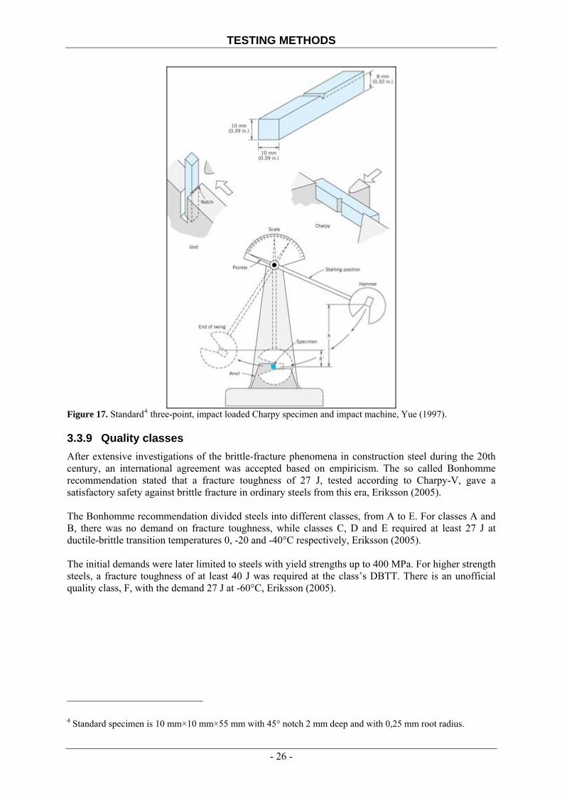
TESTING METHODS

Figure 17. Standard4 three-point, impact loaded Charpy specimen and impact machine, Yue (1997). 3.3.9 Quality classes After extensive investigations of the brittle-fracture phenomena in construction steel during the 20th century, an international agreement was accepted based on empiricism. The so called Bonhomme recommendation stated that a fracture toughness of 27 J, tested according to Charpy-V, gave a satisfactory safety against brittle fracture in ordinary steels from this era, Eriksson (2005). The Bonhomme recommendation divided steels into different classes, from A to E. For classes A and B, there was no demand on fracture toughness, while classes C, D and E required at least 27 J at ductile-brittle transition temperatures 0, -20 and -40°C respectively, Eriksson (2005). The initial demands were later limited to steels with yield strengths up to 400 MPa. For higher strength steels, a fracture toughness of at least 40 J was required at the class’s DBTT. There is an unofficial quality class, F, with the demand 27 J at -60°C, Eriksson (2005).

4 Standard specimen is 10 mm×10 mm×55 mm with 45° notch 2 mm deep and with 0,25 mm root radius.

- 26 -

THEORY

4 Theory

4.1 Static strength of welded joints

Normally the designer works under the presumption that the yield strength is the same for the weld metal and the base metal. This is, however, a truth with modification. In reality, the welded joint is made up of several, united, thin layers of various strengths. This is revealed by testing the hardness of the joint. Figure 18 shows that immediately outside the over-heated zone is a layer with very low hardness and the hardness is proportional to the ultimate strength, Hannerz (xxxx).

Figure 18. Hardness profile transverse a welded joint, SSAB Oxelösund (2007). This problem has employed scientists in both Russia and Japan, Hannerz (xxxx). If a uniaxial load is applied transverse to a butt weld the yield criteria is initially sσ=σ (4.1) when the stresses are 1σ 032 =σ=σ If there is a thin soft zone in the weld, surrounded by a harder material, this uniaxial state of stress is rapidly transformed to the multiaxial state of stress where, 321 ,, σσσ all differ from zero, Hannerz (xxxx). When this triaxial state occurs, the yield criteria is changed to s21 σ=σ−σ (4.2) Depending on that the plastic yielding is locally restrained. The global strength is so forth, in practice, higher than what is obtained by simply transcribing the lowest hardness to a yield- or ultimate strength.

- 27 -

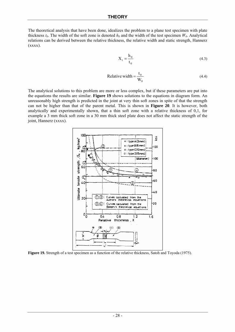
THEORY

The theoretical analysis that have been done, idealizes the problem to a plane test specimen with plate thickness t0. The width of the soft zone is denoted h0 and the width of the test specimen W0. Analytical relations can be derived between the relative thickness, the relative width and static strength, Hannerz (xxxx).

0

0t t

hX = (4.3)

0

0

Wt

widthRelative = (4.4)

The analytical solutions to this problem are more or less complex, but if these parameters are put into the equations the results are similar. Figure 19 shows solutions to the equations in diagram form. An unreasonably high strength is predicted in the joint at very thin soft zones in spite of that the strength can not be higher than that of the parent metal. This is shown in Figure 20. It is however, both analytically and experimentally shown, that a thin soft zone with a relative thickness of 0,1, for example a 3 mm thick soft zone in a 30 mm thick steel plate does not affect the static strength of the joint, Hannerz (xxxx).

Figure 19. Strength of a test specimen as a function of the relative thickness, Satoh and Toyoda (1975).

- 28 -

THEORY

Figure 20. Effect of specimen width on ultimate tensile strength, Satoh and Toyoda (1975). 4.2 Influence of heat input

The heat input is significant for how fast the weld cools and can be calculated by, Weman (2002):

60 efficiency

1000U IQv⋅ ⋅

= ⋅⋅

[kJ/mm] (4.5)

where U = voltage (V), I = current (A) and v = welding speed (mm/min). The efficiency is dependant on the welding process used with manual metal arc welding having a value of 0,75, gas metal arc welding and submerged arc welding, 0,9 and gas tungsten arc welding, 0,8. Low heat input means faster cooling. When welding thick steels with high equivalent carbon content it might be necessary to preheat the work piece to avoid cracks. Too high heat input results in a brittle weld. When welding thin plates in ordinary construction steels, a low heat input is to prefer with respect to stresses in the weld and deformations that easily can cause problems, Weman (2002). The added energy strongly influences the width of the soft zone and the heat input should, according to the analytical calculations, be crucial to the strength of the joint, Hannerz (xxxx). The width of the soft zone is actually proportional to the heat input. Practical tests have also proven that the strength of butt welded joints in QT-steels with Re = 700 MPa is sensitive to high heat input and that the failure will be localized in the soft zone. Too high heat input should, in other words, be avoided for high strength QT-steels. Extremely high energy welding methods should not be used, the steel manufacturer can normally inform about the maximum allowed heat input, Hannerz (xxxx). 4.3 Influence of the steel type

If a steel manufacturer chooses to fabricate his QT-steel with an extremely low equivalent carbon content to increase the weldability of the steel, then the steel is less usable for high energy welding. Steels that are very prone to this are the quenched (not tempered) steels. When using this type of

- 29 -

THEORY

steels, soft zones must always be taken into account, especially in an abrasive environment where hardness is of primary significance, Hannerz (xxxx). 4.4 Softer weld metal

To reduce the tendency for hydrogen cracks, a softer welding electrode can be used. This lessens the joint’s stiffness a bit and the demand for pre heating is not as strong, Hannerz (xxxx). Japanese tests have shown that from both a static and dynamic point of view, a 90 % hardness of the weld metal is acceptable. An undermatching weld in a butt joint is actually the same thing as a fairly wide soft zone, Hannerz (xxxx). 4.5 Work hardening and necking

When the stress, during a tensile test, reaches a critical level, plastic deformation (yielding) will occur at the weakest part of the test sample, somewhere along the gauge length. This local extension under tensile loading will cause a simultaneous area constriction so that the true local stress is higher at this location than anywhere else along the gauge length, Hertzberg (1983). Consequently, it would be expected that all additional deformation would concentrate in this most highly stressed region. Such is the case in an ideally plastic material. For all other materials, however, this localized plastic deformation strain hardens the material, thereby making it more resistant to further damage. At this point the applied stress must be increased to produce additional plastic deformation at the second weakest position along the gauge length. Here again the material strain hardens and the process continues. On a macroscopic scale, the gauge length extends uniformly together with a uniform reduction in cross-sectional area. (Plastic deformation is a constant volume process). With increasing load, a point is reached where the strain hardening capacity of the material is exhausted and the nth local area contraction is no longer balanced by a corresponding increase in material strength, Hertzberg (1983). At this maximum load, further plastic deformation is localized in the necked region, since the stress increases continually with areal contraction even though the applied load is decreasing as a result of elastic unloading in the test bar outside the necked area. Eventually the neck will fail, Hertzberg (1983).

1. Ultimate strength 2. Yield strength 3. Rupture 4. Strain hardening region 5. Necking region

The engineering stress-strain curve does not give a true indication of the deformation characteristics of a metal because it is based entirely on the original dimensions of the specimen, and these dimensions change continuously during the test, Key to Steel (2007). Since engineering stress is based on the original cross-sectional area, the

Figure 21. Stress vs. strain curve for a typical structural steel.

- 30 -

THEORY

decreasing load on the sample after the neck has formed (maximum load) will result in the computation of a decreasing stress, Hertzberg (1983). Actually, the metal continues to strain-harden all the way up to fracture, so that the stress required to produce further deformation should also increase. If the true stress, based on the actual cross-sectional area of the specimen, is used, it is found that the stress-strain curve increases continuously up to fracture. If the strain measurement is also based on instantaneous measurements, the curve, which is obtained, is known as a true-stress-true-strain curve. This is also known as a flow curve since it represents the basic plastic-flow characteristics of the material. Any point on the flow curve can be considered the yield stress for a metal strained in tension by the amount shown on the curve. Thus, if the load is removed at this point and then reapplied, the material will behave elastically throughout the entire range of reloading, Key to Steel (2007).

Figure 22. True-stress, true-strain curve, Key to Steel (2007) Figure 22 compares the true-stress-true-strain curve with its corresponding engineering stress-strain curve. Note that because of the relatively large plastic strains, the elastic region has been compressed into the y-axis. In agreement with equations (4.12) and (4.14) the true-stress-true-strain curve is always to the left of the engineering curve until the maximum load is reached. However, beyond maximum load the high-localized strains in the necked region far exceed the engineering strain calculated from equation (4.14). Frequently the flow curve is linear from maximum load to fracture, while in other cases its slope continuously decreases up to fracture. The formation of a necked region or mild notch introduces triaxial stresses, which make it difficult to determine accurately the longitudinal tensile stress on out to fracture, Key to Steel (2007). 4.5.1 Definitions of stress and strain The definition of the terms stress and strain may be done in two, generally accepted forms, Hertzberg (1983). The first definitions, used extensively in engineering practice, are:

0area sectional-cross initial

loadstress gengineerinAP

eng ===σ (4.6)

1length initial

lengthin changestrain gengineerin00

0

00

0 −=−=−

===ll

ll

ll

lll fff

engε (4.7)

Where lf = final gauge length l0 = initial gauge length Alternatively, stress and strain can be defined by:

- 31 -

THEORY

i

true AP

===area sectional-cross ousinstantane

loadstress trueσ (4.8)

[ ] ( ) ( )length initial

length finallnlnlnlnlnstrain true0

00

0

=⎟⎟⎠

⎞⎜⎜⎝

⎛=−==== ∫ l

llll

ldl f

fll

l

ltrue

f

f

ε (4.9)

The basic difference regarding the definitions for true stress and strain is the recognition of the relation between gauge length and diameter changes that are associated with plastic deformation, Hertzberg (1983). Because plastic deformation is a constant volume process such that constant2211 =⋅=⋅= lAlAV (4.10) an extension of the initial gauge length will produce a corresponding contraction of the gauge diameter, Hertzberg (1983). There are two examples in Appendix A to visualise the differences between true- end engineering stress and strain. The definition of true strain given in equation (4.9) makes it possible to define the strain given to a rod by considering the total change in length of the rod as having taken place in either one step or any number of steps, Hertzberg (1983). Take, for example, a wire drawn in two steps with intermediate unloading. The two deformation strains would be (l1-l0)/l0 and (l2-l1)/l1. If these two increments were added, the result would not be equal to a final strain of (l2-l0)/l0. On the other hand, summation of true strains does lead to the correct result:

tottruel

lll

ll

ε==+0

2

1

2

0

1 lnlnln (4.11)

4.5.2 Relationships between true and engineering stress and strain Equation (4.7) gives:

( ) truef

engf

eng ll

ll

εεε ==+⇒=+00

ln1ln1 (4.12)

The constant volume process implies:

( )00

0 111AAl

lAA eng

ieng

f

i

+=⇒+==ε

ε (4.13)

Which, together with the definition of true stress gives:

( ) ( 110

+=+== engengengi

true AP

AP εσεσ ) (4.14)

The derivation of the above equation assumes both constancy of volume and a homogeneous strain distribution along the gauge length of the tension specimen. Therefore, equation (4.14) should only be used until the onset of necking. Beyond maximum load, the true stress should be determined from actual measurements of load and cross-sectional area, Key to Steel (2007).

- 32 -

THEORY

The portion of the true stress-strain curve (from the onset of yielding to the maximum load) may be described empirically by the relationship generally attributed to Hollomon, Hertzberg (1983): (4.15) nK εσ ⋅= Where σ = true stress ε = true plastic strain n = strain hardening coefficient K = material constant defined as the true stress at a true strain of 1.0 The magnitude of the strain hardening coefficient reflects the ability of the material to resist further deformation. In the limit, n may be equal to unity, which represents ideally elastic behaviour, or equal to zero, which represents an ideally plastic material. Values of n are sensitive to thermo-dynamical treatment; they are generally larger for materials in the hardened condition and smaller in the cold worked state, Hertzberg (1983). The strain hardening coefficient can be derived by plotting true stress and associated true strain values on a log-log paper. If the Hollomon equation was absolutely correct, the result would be a straight line with a slope equal to n. This is, however, not always found to be the case and reflects the fact that this relationship is only an empirical approximation. If a non-linear log-log plot is the result for a given material, the strain-hardening coefficient is often defined at a particular strain value. In general, n increases with decreasing strength level and with decreasing mobility of certain dislocations in the crystalline lattice, Hertzberg (1983).

Figure 23. Log/log plot of true stress-strain curve Key to Steel (2007).

Figure 24. Various forms of power curve, nKσ ε= ⋅ Key to Steel (2007).

- 33 -

THEORY

4.5.3 Necking and triaxiality In addition to the necking strains, a triaxial stress state exists in the vicinity of the neck. The radial (σr) and transverse (σt) stresses that are induced are developed as a result of a Poisson effect. In effect, the more highly stressed material within the neck wishes to pull in to accommodate the large local extensions. Since the material immediately adjacent to the necked area experiences a much lower stress level, these regions will resist such contractions by exerting induced tensile stresses that act to retard deepening of the neck. Consequently, the triaxial stress field acts to plastically constrain the material from deforming in the reduced area. To provide for such plastic flow, the axial stress must be increased. The stress values recorded on the true stress-strain curve after the onset of necking reflect the higher axial stresses necessitated by the triaxial stress condition, Hertzberg (1983). In terms of the radius of curvature of the neck contour R and the radius of the minimum cross-sectional area a, Bridgeman was able to correct the applied axial stress (σapp) to determine the true stress (σtrue) that would be necessary to deform the material were it not for the presence of the neck, Hertzberg (1983). The corrected true stress-strain curve shown in Figure 22 can be determined from the Bridgeman relation:

( ) ( )[ ]RaaRapp

true

21ln211

++=

σσ

(4.16)

- 34 -

PREVIOUS WORK

5 Previous work

5.1 Dexter (1997)

This report discusses the behaviour and performance of structures, which can be affected by strength undermatching of welds. Data from experiments on full-scale structural elements like, for example wide-plate tests, are reviewed. The importance of strain-hardening for ductility and fracture resistance of structural members and connections is also discussed. Another interesting aspect of this paper is the discussion of which roles strain-hardening and constraint have on the ductility of undermatched welds. 5.1.1 Introduction For joints, where failure could be catastrophic, the welding-codes require the weld metal to be overmatched. This protects the weld from localized plastic strain, i.e. forces the plastic deformation to occur in the parent plate. For non-critical structural members, however, and joints subjected to certain types of loading, the welds may be undermatched. For steel with yield strength less than 500-600 MPa, the overmatching requirement in the codes presents no special problem. Strength undermatching in welds is therefore only an issue for structures made in high strength steel. The U.S. Navy uses high strength steel in their surface ships. There are two different grades, according to the military specification, known as HSLA-805 (560 MPa yield strength) and HSLA-100 (690 MPa yield strength). These steels have more stringent toughness requirements than corresponding steels intended for civil markets. The fracture properties make these steels ideal for connections where a weld, transverse to the loading direction, is loaded in tension. It is not easy, however, to find overmatching filler metals which are resistant to hydrogen-assisted cracking, for 690 MPa yield strength steel. There is a standard overmatching electrode for HSLA-100, called Mil-120 with an ultimate strength of 830 MPa. This is nominally a 10% overmatch relative to the MSYS (minimum specified yield strength) of the steel. The most commonly used undermatching wire is Mil-100S-1 (690 MPa ultimate strength). This wire’s minimum allowed yield strength is 565 MPa, which represents an 18 % (565/690) undermatch of the base metal. The 100S-1 wire could be undermatched as much as 37% (565/900), if the steel is made of the maximum allowed yield strength, which is 900 MPa. Welds that are undermatched only about 10 percent relative to the MSYS of the parent plate can easily be produced by controlling the maximum heat input and the associated minimum cooling rate. Because of the 120S-1 wire’s higher carbon and alloy levels, it is much more susceptible to hydrogen-assisted cracking and consequently requires stringent preheating. The 100S-1 wire, on the other hand, can be used without or only with minimal preheat. The undermatching filler metal does not only have better weldability, but also has 50 percent higher notch toughness at service temperatures. These advantages reduces welding costs and results in a joint with improved fracture resistance, when using a moderately undermatched 100S-1 electrode. In real welding-applications, there is a great probability of unintentional undermatching when the actual yield strengths of the weld- and base metals are not known. If the plate has higher strength than the MSYS, welds can unknowingly be undermatched. According to the specification, the yield

5 80 ksi = 551,6 MPa

- 35 -

PREVIOUS WORK

strength for HSLA-100 should remain in range 690-900 MPa, for example. Tensile test data from the steel mills shows that the mean yield strength is 745 MPa and the coefficient of variation is about 5,5 %. In addition to higher yield strength of the parent metal, the weld filler metal may have lower strength than expected. The weld metal certification tests are often performed in thicker plates than the application, which implies that the cooling rate and consequently the strength could be lower in the application. Weld undermatch in a relatively thin plate has, for example, been examined in a study at General Dynamics Boat Division. Fifty-four specimens were fabricated in HY-100 steel (690 MPa MSYS) with overmatching 120S-1 welding wires using thicknesses between 9 and 16 mm and several weld processes. Table 2. Tensile tests for welding of thin plates with Mil-120S-1 Thickness [mm] Welding process Number of Specimens Avg. YS [MPa] Avg. TS [MPa]

SMAW 10 613 756 9 GMAW 6 702 819 P-GMAW 6 630 825 SMAW 8 633 763

13 GMAW 6 657 798 P-GMAW 6 596 814 SMAW 3 653 752

16 GMAW 5 704 817 P-GMAW 4 659 821

All Specimens 54 645 793 Table 2 shows that only 11 % of the specimens achieved the required 704 MPa yield strength and that the average was almost 60 MPa under that value, which represents an undermatch of 6-7 percent relative to the MSYS. Shielded metal arc welding (SMAW) in 9 mm thick plate produced the lowest weld metal strength, where the average yield strength was 613 MPa. The important parameter is the undermatch relative to actual yield strengths. Unintentional undermatched welds are a potential hazard without guidelines governing their impact on structural performance. 5.1.2 Structural requirements Of the primary structural requirements (stiffness, strength, ductility, resistance to corrosion, fatigue resistance and fracture resistance), undermatched welds only have a significant effect on the strength, fracture resistance and ductility of structures. Undermatched welds have no effect on fatigue strength, according to earlier studies. The strength may be limited by:

1. Gross-section yielding (GSY) in tension or shear 2. Buckling from compression, shear or bending 3. Fracture in tension or shear

Buckling will, in thin-plate structures, initiate in the elastic range and should therefore not be significantly affected by undermatched welds. Research indicates that the buckling-strength of even thicker plates is not adversely affected by undermatching.

- 36 -

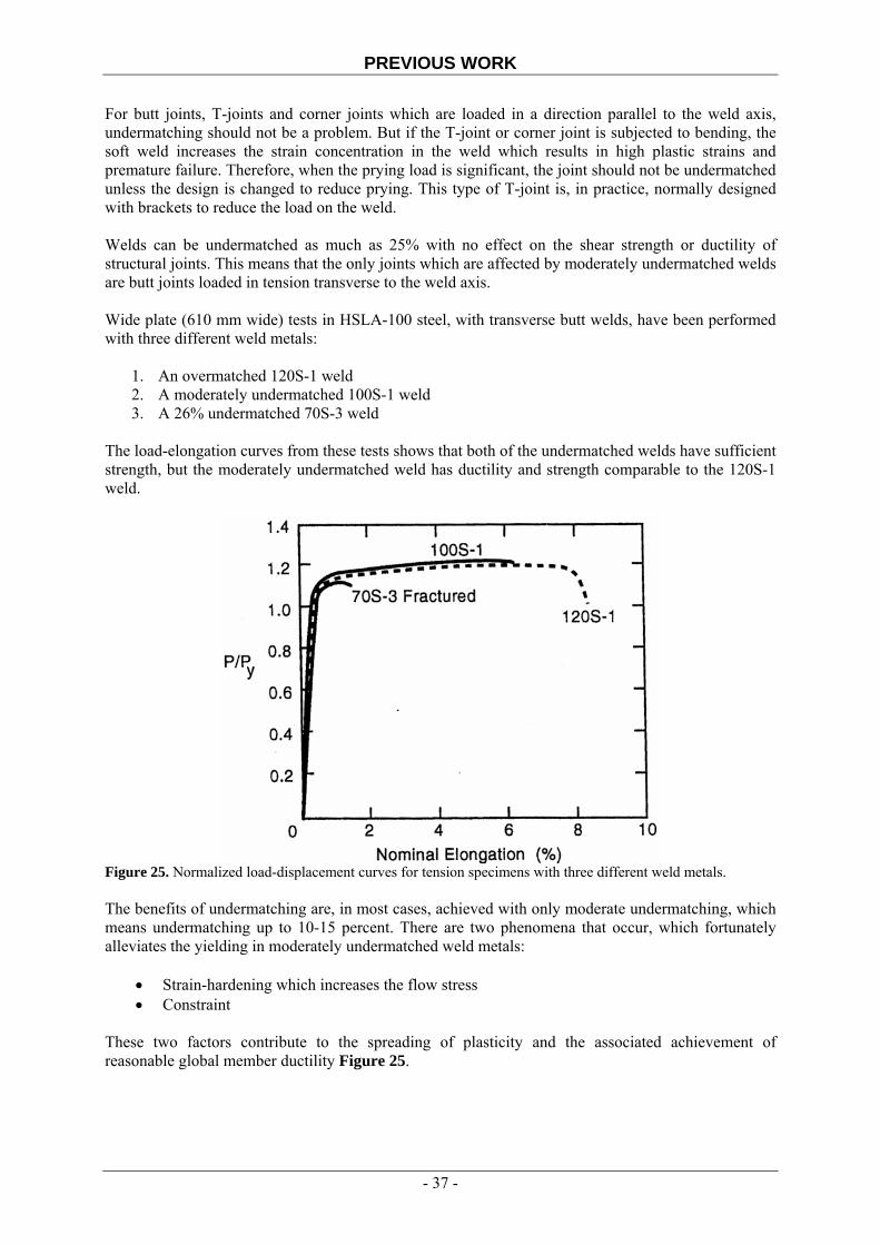
PREVIOUS WORK

For butt joints, T-joints and corner joints which are loaded in a direction parallel to the weld axis, undermatching should not be a problem. But if the T-joint or corner joint is subjected to bending, the soft weld increases the strain concentration in the weld which results in high plastic strains and premature failure. Therefore, when the prying load is significant, the joint should not be undermatched unless the design is changed to reduce prying. This type of T-joint is, in practice, normally designed with brackets to reduce the load on the weld. Welds can be undermatched as much as 25% with no effect on the shear strength or ductility of structural joints. This means that the only joints which are affected by moderately undermatched welds are butt joints loaded in tension transverse to the weld axis. Wide plate (610 mm wide) tests in HSLA-100 steel, with transverse butt welds, have been performed with three different weld metals:

1. An overmatched 120S-1 weld 2. A moderately undermatched 100S-1 weld 3. A 26% undermatched 70S-3 weld

The load-elongation curves from these tests shows that both of the undermatched welds have sufficient strength, but the moderately undermatched weld has ductility and strength comparable to the 120S-1 weld.

Figure 25. Normalized load-displacement curves for tension specimens with three different weld metals. The benefits of undermatching are, in most cases, achieved with only moderate undermatching, which means undermatching up to 10-15 percent. There are two phenomena that occur, which fortunately alleviates the yielding in moderately undermatched weld metals:

• Strain-hardening which increases the flow stress • Constraint

These two factors contribute to the spreading of plasticity and the associated achievement of reasonable global member ductility Figure 25.

- 37 -

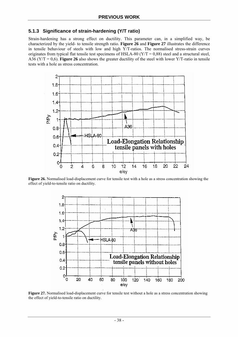
PREVIOUS WORK

5.1.3 Significance of strain-hardening (Y/T ratio) Strain-hardening has a strong effect on ductility. This parameter can, in a simplified way, be characterized by the yield- to tensile strength ratio. Figure 26 and Figure 27 illustrates the difference in tensile behaviour of steels with low and high Y/T-ratios. The normalised stress-strain curves originates from typical flat tensile test specimens of HSLA-80 (Y/T = 0,88) steel and a structural steel, A36 (Y/T = 0,6). Figure 26 also shows the greater ductility of the steel with lower Y/T-ratio in tensile tests with a hole as stress concentration.

Figure 26. Normalised load-displacement curve for tensile test with a hole as a stress concentration showing the effect of yield-to-tensile ratio on ductility.

Figure 27. Normalised load-displacement curve for tensile test without a hole as a stress concentration showing the effect of yield-to-tensile ratio on ductility.

- 38 -

PREVIOUS WORK

With undermatched welds, the situation is similar to that of the net section of bolted joints. The gross section is inherently stronger because of the decreased cross-sectional area of the plane that contains the bolt holes. If ductile gross-section failure is desired, in bolt-joint design, the ratio of the net- to gross sectional area can not be less than the Y/T-ratio of the steel. The strain-hardening effect is counted on to delay the localization of strain in the net section until the gross section has yielded. For bolted joints in high-strength A514 (690 MPa MSYS) steel with a Y/T-ratio of about 0,93, the minimum ratio of net- to gross area must exceed 0,87 if the undesirable net section failure mode with low ductility is to be avoided. The minimum allowable ratio of net- to gross area is slightly smaller than what it would be if only strain-hardening was accounted for. The additional effect is probably due to constraint. A design approach which ignores the constraint-effect is on the conservative side in this case. In earlier days, when the majority of structural codes were developed often based on full-scale tests, most of the structural steels had a low Y/T-ratio (below 0,75). With today’s structural steel, from electrical furnaces that allows unintentional alloying, the Y/T-ratio is much higher. It is, in fact, possible to find ordinary structural steel (350 MPa MSYS) with a Y/T-ratio that exceeds 0,9 nowadays. It is not completely clear if these high Y/T-ratio steels will behave in the way that the codes anticipate. Beyond a certain level of toughness, the yield-to-tensile strength ratio of the steel or weld metal, has a greater effect on ductility than that of increased toughness. The plastic deformation can be spread away from a notch or a crack in a steel or a weld metal with a Y/T-ratio lower than 0,8. This means that gross-section yielding can develop resulting in increased overall elongation. Steel or weld metal which has higher Y/T-ratios, tend to concentrate the plastic deformation to a narrow band close to the notch or the crack. The typical Charpy V-notch (CVN) and fracture toughness test (J/CTOD) specimen are too small and deeply notched to develop the benefit of gross-section yielding that a low Y/T-ratio promotes. This is why these tests do not show much difference between steel or weld metals with widely varying Y/T-ratios.

Figure 28. Experimental load-deflection curves for the HSLA-80 and EH36 CCT specimens. Displacement was measured over a 460 mm gauge length.

- 39 -

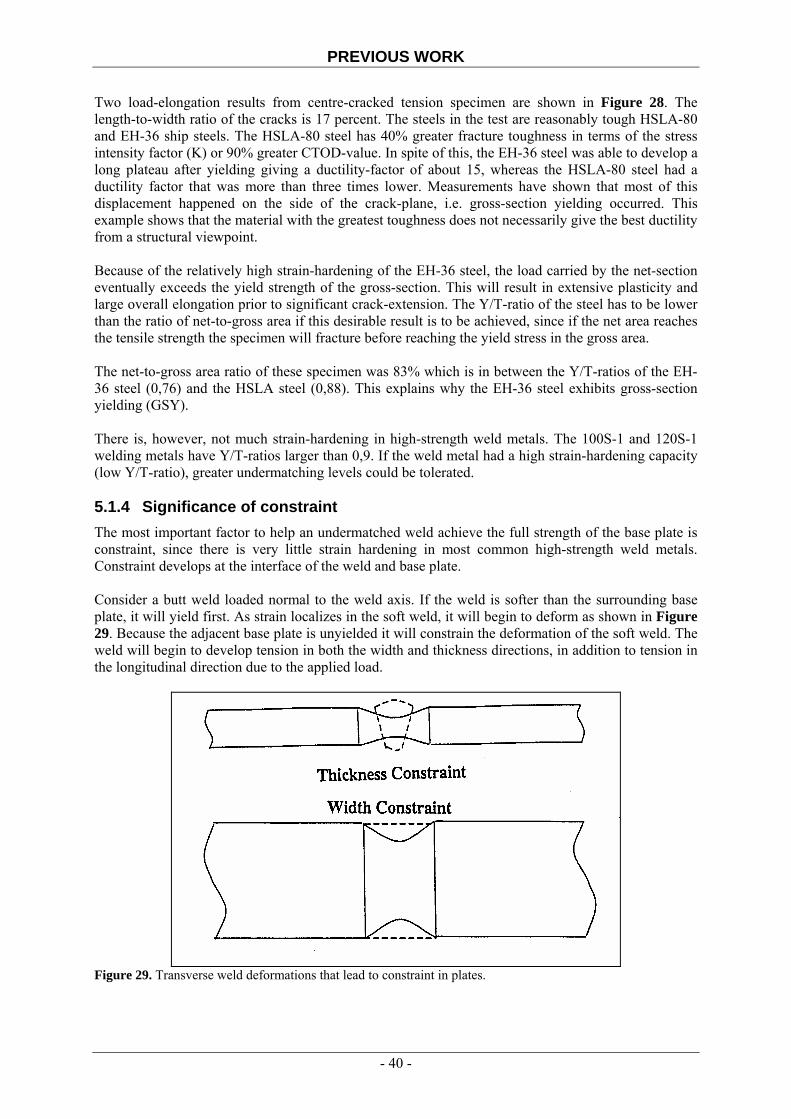
PREVIOUS WORK

Two load-elongation results from centre-cracked tension specimen are shown in Figure 28. The length-to-width ratio of the cracks is 17 percent. The steels in the test are reasonably tough HSLA-80 and EH-36 ship steels. The HSLA-80 steel has 40% greater fracture toughness in terms of the stress intensity factor (K) or 90% greater CTOD-value. In spite of this, the EH-36 steel was able to develop a long plateau after yielding giving a ductility-factor of about 15, whereas the HSLA-80 steel had a ductility factor that was more than three times lower. Measurements have shown that most of this displacement happened on the side of the crack-plane, i.e. gross-section yielding occurred. This example shows that the material with the greatest toughness does not necessarily give the best ductility from a structural viewpoint. Because of the relatively high strain-hardening of the EH-36 steel, the load carried by the net-section eventually exceeds the yield strength of the gross-section. This will result in extensive plasticity and large overall elongation prior to significant crack-extension. The Y/T-ratio of the steel has to be lower than the ratio of net-to-gross area if this desirable result is to be achieved, since if the net area reaches the tensile strength the specimen will fracture before reaching the yield stress in the gross area. The net-to-gross area ratio of these specimen was 83% which is in between the Y/T-ratios of the EH-36 steel (0,76) and the HSLA steel (0,88). This explains why the EH-36 steel exhibits gross-section yielding (GSY). There is, however, not much strain-hardening in high-strength weld metals. The 100S-1 and 120S-1 welding metals have Y/T-ratios larger than 0,9. If the weld metal had a high strain-hardening capacity (low Y/T-ratio), greater undermatching levels could be tolerated. 5.1.4 Significance of constraint The most important factor to help an undermatched weld achieve the full strength of the base plate is constraint, since there is very little strain hardening in most common high-strength weld metals. Constraint develops at the interface of the weld and base plate. Consider a butt weld loaded normal to the weld axis. If the weld is softer than the surrounding base plate, it will yield first. As strain localizes in the soft weld, it will begin to deform as shown in Figure 29. Because the adjacent base plate is unyielded it will constrain the deformation of the soft weld. The weld will begin to develop tension in both the width and thickness directions, in addition to tension in the longitudinal direction due to the applied load.

Figure 29. Transverse weld deformations that lead to constraint in plates.

- 40 -

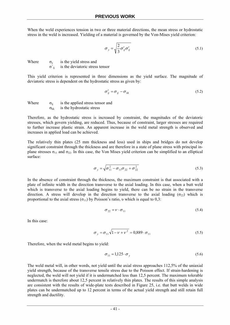
PREVIOUS WORK

When the weld experiences tension in two or three material directions, the mean stress or hydrostatic stress in the weld is increased. Yielding of a material is governed by the Von-Mises yield criterion:

ijijy σσσ ′′=32

(5.1)

Where σy is the yield stress and σ´ij is the deviatoric stress tensor This yield criterion is represented in three dimensions as the yield surface. The magnitude of deviatoric stress is dependent on the hydrostatic stress as given by: kkijij σσσ −=′ (5.2)

Where σij is the applied stress tensor and σkk is the hydrostatic stress Therefore, as the hydrostatic stress is increased by constraint, the magnitudes of the deviatoric stresses, which govern yielding, are reduced. Thus, because of constraint, larger stresses are required to further increase plastic strain. An apparent increase in the weld metal strength is observed and increases in applied load can be achieved. The relatively thin plates (25 mm thickness and less) used in ships and bridges do not develop significant constraint through the thickness and are therefore in a state of plane stress with principal in-plane stresses σ11 and σ22. In this case, the Von Mises yield criterion can be simplified to an elliptical surface: 2

222211211 σσσσσ +−=y (5.3)

In the absence of constraint through the thickness, the maximum constraint is that associated with a plate of infinite width in the direction transverse to the axial loading. In this case, when a butt weld which is transverse to the axial loading begins to yield, there can be no strain in the transverse direction. A stress will develop in the direction transverse to the axial loading (σ22) which is proportional to the axial stress (σ11) by Poisson’s ratio, υ which is equal to 0,3: 1122 σνσ ⋅= (5.4) In this case: 11

211 889,01 σννσσ ⋅=+−=y (5.5)

Therefore, when the weld metal begins to yield: yσσ ⋅= 125,111 (5.6)

The weld metal will, in other words, not yield until the axial stress approaches 112,5% of the uniaxial yield strength, because of the transverse tensile stress due to the Poisson effect. If strain-hardening is neglected, the weld will not yield if it is undermatched less than 12,5 percent. The maximum tolerable undermatch is therefore about 12,5 percent in relatively thin plates. The results of this simple analysis are consistent with the results of wide-plate tests described in Figure 25, i.e. that butt welds in wide plates can be undermatched up to 12 percent in terms of the actual yield strength and still retain full strength and ductility.

- 41 -

PREVIOUS WORK

Higher levels of undermatching can be tolerated in thicker sections due to the development of through-thickness constraint. But, because of the potential problems with brittle fracture of thick section weldments and how constraint adversely affects the potential for brittle fracture, the development of through-thickness constraint must be viewed with great caution. If sufficient constraint can be developed, yielding will eventually spread outside the soft weld which means that gross-section yielding of the weldment will be reached. When GSY is achieved, the full base plate strength and significant ductility is also achieved, even with an undermatched weld. 5.1.5 Effect of weld defects and cracks Fracture research indicates that there is a significant effect of undermatching on wide-plate tests with transverse through-thickness or surface-cracks along the centreline of the weld. These results have led to a general reluctance to accept undermatched welds. This specimen geometry is, however, not realistic. Most welding cracks occur along the fusion line or in the HAZ. Fatigue cracks occur at the weld toe and typically propagate in the HAZ. There is, in fact, research that shows that undermatching has relatively little effect on cracks near the fusion-line, compared to cracks at the weld centreline. In 1993, the first international symposium on Mis-matching of welds concluded, that undermatching was considered to have an effect, if the total elongation of the wide-plate test was significantly reduced for undermatched welds compared to overmatched ones. The consensus was that undermatching had a significant effect for small cracks in the middle of the weld. There was typically no undermatching effect for the following conditions:

a) Cracks on the fusion line b) Surface cracks at the root of single-V groove welds c) Large cracks, i.e. through cracks greater than 25 percent of the width or surface cracks greater

than 15 percent of the area d) Cracks in welds subjected to a strain gradient, such as near a stress concentration or for

members in bending e) Cleavage fracture which occurs below the weld yield strength

5.1.6 Conclusions The only welds of concern for undermatching are butt welds loaded in tension perpendicular to the weld axis. These critical welds can be undermatched up to 25% and still achieve the full yield strength of the base plate. The ductility and fracture resistance will, however, be compromised at this level of undermatching. Transverse butt welds without reinforcement in wide panels can tolerate undermatching up to 12% without loss of strength and ductility. This is fortunate, because there are indications that despite the prescription of weld metal which is nominally overmatched, unintentional undermatching may still occur in high-strength steel structures. When this possible undermatch is compounded by intentionally undermatching up to 10 percent nominally, special attention must be given to verification of actual weld metal strength and base metal strength. 5.2 Loureiro (2002)

The aim of this work was to study the effect of the welding procedure on the microstructure and mechanical properties of undermatched welds and analyze its influence on the performance under tension of the welded joint. Two different heat inputs were used in order to obtain distinct mechanical properties in the weld metal (WM) and the heat-affected zone (HAZ) of the welds.

- 42 -

PREVIOUS WORK

5.2.1 Experimental procedure Welds were produced in 25 mm thick coupon plates of high strength quenched and tempered steel (RQT 701-British Steel). A K-type joint preparation was used and welds were performed transversely to the rolling direction. Two soft root beads were executed in each coupon plate by manual metal arc, before automatic welding. After this submerged arc welds were produced with heat inputs of 2 kJ/mm (reference R2) and 5 kJ/mm (reference R5). Thermal cycles, microstructures, hardness and tensile properties were studied and evaluated. Tensile specimens sampling the WM, the WM and HAZ together (WH) and both zones and the base material (WHB) were extracted. The specimens were cylindrical with 8 mm diameter and 12,5 mm gauge length for zones W and WH. For zones WHB and the base material, the gauge length was 50 mm. 5.2.2 Results and discussion

5.2.2.1 Thermal cycles Two thermal cycle curves were obtained for the coarse grained heat-affected zone; one for 2 kJ/mm and one for 5 kJ/mm heat input. The peak temperature in each case was 1350˚C and the cooling time between 800 and 500˚C (Δt8-5) was 6 and 28 s respectively. A significant decrease in the cooling rate was observed with the increase of heat input. The time spent above 1000˚C increased from 3 s to 8 s. A change of the slope of the curve reveals a phase transformation. With increasing heat input the phase transformation temperatures increases, suggesting changes in the microstructures obtained in each case. The starting and ending temperature of phase transformation for the different heat inputs are:

490T 2Rs = ˚C ˚C 385T 2R

f =

560T 5Rs = ˚C ˚C 450T 2R

f =

5.2.2.2 Microstructures The microstructure of the deposited WM was mainly composed of acicular ferrite, with some islands of primary ferrite. A slight coarsening of the microstructure with the increase of heat input could be observed in micrographs. The austenite grain size (γ g.s.) was measured in the CGHAZ of the welds near the fusion line. A substantial growth was obtained with increasing heat input. The grain sizes were measured following a line parallel to the fusion line at a distance of 50 μm from it;

γ g.sR2 = 36 ± 4 μm γ g.sR5 = 83 ± 6 μm

The grain size of the parent plate was 12,5 ± 2 μm. The increase of heat input and consequently the time above 1000˚C and the cooling time, promotes the formation and coarsening of upper bainite and even the appearance of some ferrite side plates.

5.2.2.3 Hardness Vickers hardness indentations were made, using a 1 kg load along a line parallel to the plate surface and situated 6 mm beneath the surface. Hardness was also measured in the WM, through the thickness. The increase of heat input induced a marked decrease of hardness in the WM and HAZ of the welds. This reduction may be associated to the microstructural changes observed in these zones. In the WM

- 43 -

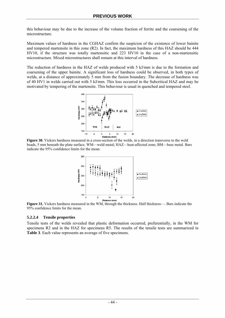
PREVIOUS WORK

this behaviour may be due to the increase of the volume fraction of ferrite and the coarsening of the microstructure. Maximum values of hardness in the CGHAZ confirm the suspicion of the existence of lower bainite and tempered martensite in this zone (R2). In fact, the maximum hardness of this HAZ should be 444 HV10, if the structure was totally martensitic and 223 HV10 in the case of a non-martensitic microstructure. Mixed microstructures shall remain at this interval of hardness. The reduction of hardness in the HAZ of welds produced with 5 kJ/mm is due to the formation and coarsening of the upper bainite. A significant loss of hardness could be observed, in both types of welds, at a distance of approximately 5 mm from the fusion boundary. The decrease of hardness was of 40 HV1 in welds carried out with 5 kJ/mm. This loss occurred in the Subcritical HAZ and may be motivated by tempering of the martensite. This behaviour is usual in quenched and tempered steel.

Figure 30. Vickers hardness measured in a cross-section of the welds, in a direction transverse to the weld beads, 5 mm beneath the plate surface. WM—weld metal; HAZ—heat-affected zone; BM—base metal. Bars indicate the 95% confidence limits for the mean.

Figure 31. Vickers hardness measured in the WM, through the thickness. Half thickness—. Bars indicate the 95% confidence limits for the mean.

5.2.2.4 Tensile properties Tensile tests of the welds revealed that plastic deformation occurred, preferentially, in the WM for specimens R2 and in the HAZ for specimens R5. The results of the tensile tests are summarized in Table 3. Each value represents an average of five specimens.

- 44 -

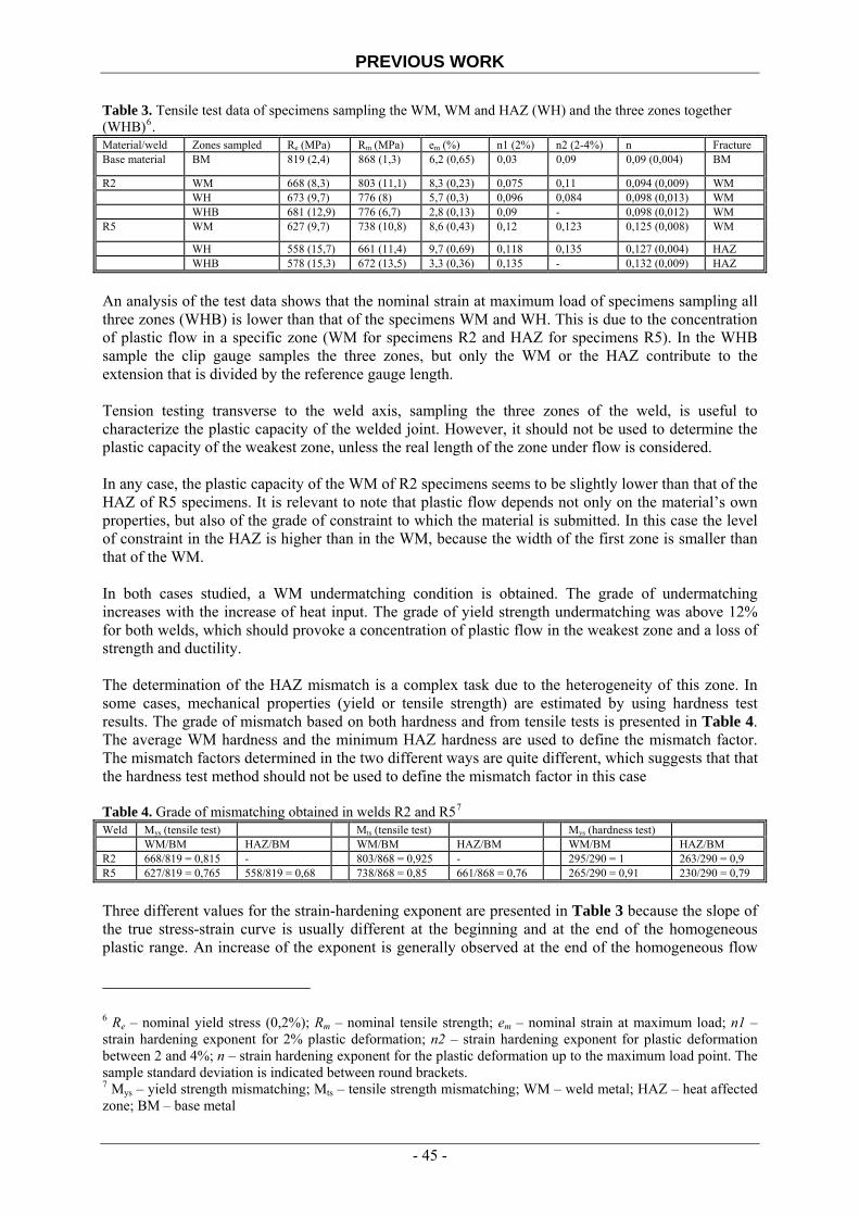
PREVIOUS WORK

Table 3. Tensile test data of specimens sampling the WM, WM and HAZ (WH) and the three zones together (WHB)6. Material/weld Zones sampled Re (MPa) Rm (MPa) em (%) n1 (2%) n2 (2-4%) n Fracture Base material BM 819 (2,4) 868 (1,3) 6,2 (0,65) 0,03 0,09 0,09 (0,004) BM

R2 WM 668 (8,3) 803 (11,1) 8,3 (0,23) 0,075 0,11 0,094 (0,009) WM WH 673 (9,7) 776 (8) 5,7 (0,3) 0,096 0,084 0,098 (0,013) WM WHB 681 (12,9) 776 (6,7) 2,8 (0,13) 0,09 - 0,098 (0,012) WM R5 WM 627 (9,7) 738 (10,8) 8,6 (0,43) 0,12 0,123 0,125 (0,008) WM

WH 558 (15,7) 661 (11,4) 9,7 (0,69) 0,118 0,135 0,127 (0,004) HAZ WHB 578 (15,3) 672 (13,5) 3,3 (0,36) 0,135 - 0,132 (0,009) HAZ

An analysis of the test data shows that the nominal strain at maximum load of specimens sampling all three zones (WHB) is lower than that of the specimens WM and WH. This is due to the concentration of plastic flow in a specific zone (WM for specimens R2 and HAZ for specimens R5). In the WHB sample the clip gauge samples the three zones, but only the WM or the HAZ contribute to the extension that is divided by the reference gauge length. Tension testing transverse to the weld axis, sampling the three zones of the weld, is useful to characterize the plastic capacity of the welded joint. However, it should not be used to determine the plastic capacity of the weakest zone, unless the real length of the zone under flow is considered. In any case, the plastic capacity of the WM of R2 specimens seems to be slightly lower than that of the HAZ of R5 specimens. It is relevant to note that plastic flow depends not only on the material’s own properties, but also of the grade of constraint to which the material is submitted. In this case the level of constraint in the HAZ is higher than in the WM, because the width of the first zone is smaller than that of the WM. In both cases studied, a WM undermatching condition is obtained. The grade of undermatching increases with the increase of heat input. The grade of yield strength undermatching was above 12% for both welds, which should provoke a concentration of plastic flow in the weakest zone and a loss of strength and ductility. The determination of the HAZ mismatch is a complex task due to the heterogeneity of this zone. In some cases, mechanical properties (yield or tensile strength) are estimated by using hardness test results. The grade of mismatch based on both hardness and from tensile tests is presented in Table 4. The average WM hardness and the minimum HAZ hardness are used to define the mismatch factor. The mismatch factors determined in the two different ways are quite different, which suggests that that the hardness test method should not be used to define the mismatch factor in this case Table 4. Grade of mismatching obtained in welds R2 and R57

Weld Mys (tensile test) Mts (tensile test) Mys (hardness test) WM/BM HAZ/BM WM/BM HAZ/BM WM/BM HAZ/BM R2 668/819 = 0,815 - 803/868 = 0,925 - 295/290 = 1 263/290 = 0,9 R5 627/819 = 0,765 558/819 = 0,68 738/868 = 0,85 661/868 = 0,76 265/290 = 0,91 230/290 = 0,79

Three different values for the strain-hardening exponent are presented in Table 3 because the slope of the true stress-strain curve is usually different at the beginning and at the end of the homogeneous plastic range. An increase of the exponent is generally observed at the end of the homogeneous flow

6 Re – nominal yield stress (0,2%); Rm – nominal tensile strength; em – nominal strain at maximum load; n1 – strain hardening exponent for 2% plastic deformation; n2 – strain hardening exponent for plastic deformation between 2 and 4%; n – strain hardening exponent for the plastic deformation up to the maximum load point. The sample standard deviation is indicated between round brackets. 7 Mys – yield strength mismatching; Mts – tensile strength mismatching; WM – weld metal; HAZ – heat affected zone; BM – base metal

- 45 -

PREVIOUS WORK

range. The strain-hardening rate (n), evaluated between the yield point and the maximum load point is frequently used when assessing these structures. Table 3 shows that there is only a slight difference between the n-value obtained in a specimen sampling the zone under plastic flow and that of the specimen sampling the zones of the weld altogether (for R2 nWM = 0,094 and nWHB = 0,098; for R5 nWH = 0,127 and nWHB = 0,132). According to these results the n-value obtained in tension tests, perpendicular to the weld axis, may be used to characterize the weakest material of undermatched welds. The strain-hardening exponent n of R5 specimens is higher than that of R2 specimens, suggesting larger plastic capacity of the HAZ of R5 than the WM of R2. A larger undermatching may be tolerated if the material suffering plastic flow has a high strain-hardening rate. This is due to the hardening of the material and the spread of plastic flow to the adjacent one. In R5 welds, the weakest material is the HAZ, which has an n of approximately 0,13, that is enough to allow the transfer of part of the plastic deformation to the WM. The tensile strength of the HAZ is higher than the yield strength of the adjacent WM. 5.2.3 Conclusions The following conclusions may be drawn from the results presented above:

• The increase of heat input produces a coarsening of the microstructure of both the WM and HAZ.

• A loss of hardness was also observed in the subcritical zone, probably due to carbide precipitation.

• The increase of heat input increases the yield and tensile strength undermatching of the WM and HAZ.

• The WM yield strength undermatching induces a concentration of plastic flow in the weakest zone and a loss of strength and ductility of the weld when loaded in tension.

• The hardness test method should not be used to define the mismatch factor of several zones of the weld.

5.3 Fernandes et al. (2004)

In this study, the influence of mismatch between material properties and constraint on the plastic deformation behaviour of the heat affected zone of welds in high-strength steels is investigated, using finite element simulations. Numerical results of tensile tests of welded samples with different hypothetical widths for the heat affected zone and various material mismatch levels are shown. The analysis concerns the overall strength and ductility of the joint in relation to the plastic behaviour of the heat affected zone. The influence of the yield strength, tensile strength and constraint on the stress and plastic strain distribution in the soft heat affected zone is also discussed. 5.3.1 Introduction In a defect-free weld, global mechanical behaviour depends on the mismatch in mechanical properties between the different welded zones, its dimension and loading mode. To ensure good tensile performance of joints, the manufacturers use a welding overmatch approach. When the overmatching requirement is achieved, a soft structure can appear in the HAZ. The mechanical properties in this zone can drastically differ from the unaffected base metal depending on the heating and cooling conditions imposed by the welding process and on the structure and chemical composition of the base plate. This is current in high strength steels for which slow cooling rates can cause a considerable loss in the yield strength of the base plate.

- 46 -

PREVIOUS WORK

In this context, it is important to determine the influence of the presence of a soft material on the overall mechanical behaviour of the joint. However, the experimental analysis of the stress-strain distribution in a welded joint is a very difficult task. The non-linearities involved in the process, such as the different elasto-plastic behaviour of the various welded zones, its geometries, the non-homogeneous strain and stress distribution makes all possible experimental analysis very complicated. Using numerical simulation, it is possible to analyse individually the various phenomena that occur in a tensile test of a welded joint. The main purpose of this work is to evaluate the influence of the degree of mismatch of material properties and the size of the HAZ on the plastic behaviour observed in tension of defect-free welded plates. The local and overall plastic behaviour of the joint is studied by modelling an arbitrarily chosen material for the HAZ and progressively changing the width of this zone. The influence of material mismatch is studied simulating various hypothetical materials for the same HAZ dimensions. 5.3.2 Procedure In order to determine the influence of the mismatch in material properties in the plastic deformation behaviour of the welded joints, several numerical simulations of tensile tests were performed. Finite element meshes with three different material domains that represent the WM, BM and HAZ were used. For the WM and BM the same mechanical properties were considered, representing an evenmatch joint with 700 MPa yield strength and hardening coefficient, n = 0,08. Table 5 summarises the mechanical properties of the HAZ and values of yield strength mismatch (MYS = Y0

HAZ/Y0ADJ) and

tensile strength mismatch (MTS = YmaxHAZ/Ymax

ADJ) relative to the adjacent materials (WM and BM) studied in this work. In this text the term undermatching is used when the mismatch parameters M < 1, evenmatch when M ≈ 1 and overmatching when M > 1. Table 5. Material properties and strength mismatch ratios. [MPa] MTS

HAZ0Y MYS (n =0,08) (n = 0,1) (n = 0,12) (n = 0,14) (n = 0,16)

400 0,57 0,65 0,71 0,79 0,88 0,98 500 0,71 0,81 0,89 0,99 1,10 1,23 600 0,86 0,97 1,07 1,19 - - Figure 32, Figure 33 and Figure 34 presents the stress-strain curves for the various HAZ materials studied. From these curves it is possible to perform an analysis of the mechanical behaviour of the materials of the joint. For example, for the HAZ material with 400 MPa yield strength, the figure indicates yield and tensile strength undermatch (MYS and MTS < 1, see Table 5) for all hardening values, except n = 0,16, that represents tensile strength evenmatch (MTS ≈ 1). For the hardening values 0.08, 0.10 and 0.12 the maximum load of the HAZ material is lower than the yield stress of the adjacent materials, but for n = 0.14 and n = 0.16 yielding of the adjacent materials must occur before the maximum load is reached in the HAZ material. When the HAZ materials have 500 and 600 MPa yield strengths, yielding of the adjacent materials is possible in all situations, except for Y0

HAZ = 500 MPa with n = 0.08. For (Y0HAZ = 500, n = 0.14 and

0.16) and (Y0HAZ = 600, n = 0.10 and 0.12) the maximum load is lowest for the WM and BM

presenting tensile strength overmatch in the HAZ (MTS > 1). It is important to enhance the materials (Y0

HAZ = 400, n = 0.16), (Y0HAZ = 500, n = 0.12) and (Y0

HAZ = 600, n = 0.08) which represents the tensile strength evenmatch situations (MTS ≈ 1).

- 47 -

PREVIOUS WORK

Figure 32. Stress-strain curves corresponding to the mechanical behaviour of the various welding zones. The grey curve corresponds to the mechanical behaviour of the adjacent materials (BM and WM) and the black curves represent hypothetical conditions studied for HAZ materials. Y0

HAZ = 400 MPa

Figure 33. Stress-strain curves corresponding to the mechanical behaviour of the various welding zones. The grey curve corresponds to the mechanical behaviour of the adjacent materials (BM and WM) and the black curves represent hypothetical conditions studied for HAZ materials. Y0

HAZ = 500 MPa

Figure 34. Stress-strain curves corresponding to the mechanical behaviour of the various welding zones. The grey curve corresponds to the mechanical behaviour of the adjacent materials (BM and WM) and the black curves represent hypothetical conditions studied for HAZ materials. Y0

HAZ = 600 MPa

In order to regard the influence of the HAZ size in the geometrical constraint effect and consequently in the mechanical behaviour of the joint, various HAZ widths (lHAZ) were represented in the finite element meshes used in the numerical simulations. These meshes represent samples with a square cross section (6.125·6.125 mm2). As the ratio of the width of the softened zone to the plate thickness (lHAZ/e) is an important parameter characterising the change of strength in the joint, in the present study it covers the range 1/6 to 1. Table 6 shows the various HAZ widths studied in the present work.

- 48 -

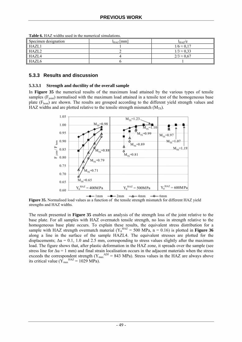
PREVIOUS WORK

Table 6. HAZ widths used in the numerical simulations. Specimen designation lHAZ [mm] lHAZ/e HAZL1 1 1/6 ≈ 0,17 HAZL2 2 1/3 ≈ 0,33 HAZL4 4 2/3 ≈ 0,67 HAZL6 6 1 5.3.3 Results and discussion

5.3.3.1 Strength and ductility of the overall sample In Figure 35 the numerical results of the maximum load attained by the various types of tensile samples (Fjoint) normalised with the maximum load attained in a tensile test of the homogeneous base plate (Fhom) are shown. The results are grouped according to the different yield strength values and HAZ widths and are plotted relative to the tensile strength mismatch (MTS).

Figure 35. Normalised load values as a function of the tensile strength mismatch for different HAZ yield strengths and HAZ widths.

The result presented in Figure 35 enables an analysis of the strength loss of the joint relative to the base plate. For all samples with HAZ overmatch tensile strength, no loss in strength relative to the homogeneous base plate occurs. To explain these results, the equivalent stress distribution for a sample with HAZ strength overmatch material (Y0

HAZ = 500 MPa, n = 0.16) is plotted in Figure 36 along a line in the surface of the sample HAZL4. The equivalent stresses are plotted for the displacements; Δu = 0.1, 1.0 and 2.5 mm, corresponding to stress values slightly after the maximum load. The figure shows that, after plastic deformation in the HAZ zone, it spreads over the sample (see stress line for Δu = 1 mm) and final strain localisation occurs in the adjacent materials when the stress exceeds the correspondent strength (Ymax

ADJ = 843 MPa). Stress values in the HAZ are always above its critical value (Ymax

HAZ = 1029 MPa).

- 49 -

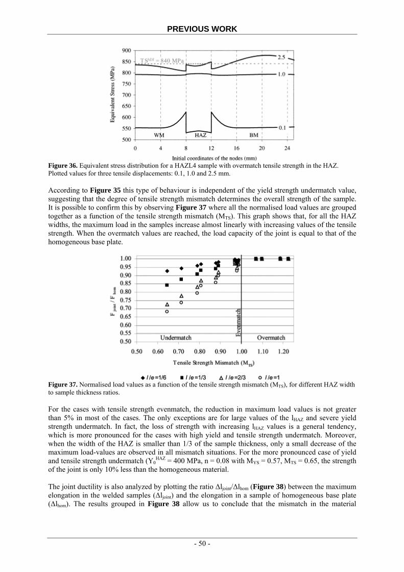
PREVIOUS WORK

Figure 36. Equivalent stress distribution for a HAZL4 sample with overmatch tensile strength in the HAZ. Plotted values for three tensile displacements: 0.1, 1.0 and 2.5 mm.

According to Figure 35 this type of behaviour is independent of the yield strength undermatch value, suggesting that the degree of tensile strength mismatch determines the overall strength of the sample. It is possible to confirm this by observing Figure 37 where all the normalised load values are grouped together as a function of the tensile strength mismatch (MTS). This graph shows that, for all the HAZ widths, the maximum load in the samples increase almost linearly with increasing values of the tensile strength. When the overmatch values are reached, the load capacity of the joint is equal to that of the homogeneous base plate.

Figure 37. Normalised load values as a function of the tensile strength mismatch (MTS), for different HAZ width to sample thickness ratios.

For the cases with tensile strength evenmatch, the reduction in maximum load values is not greater than 5% in most of the cases. The only exceptions are for large values of the lHAZ and severe yield strength undermatch. In fact, the loss of strength with increasing lHAZ values is a general tendency, which is more pronounced for the cases with high yield and tensile strength undermatch. Moreover, when the width of the HAZ is smaller than 1/3 of the sample thickness, only a small decrease of the maximum load-values are observed in all mismatch situations. For the more pronounced case of yield and tensile strength undermatch (Y0

HAZ = 400 MPa, n = 0.08 with MYS = 0.57, MTS = 0.65, the strength of the joint is only 10% less than the homogeneous material. The joint ductility is also analyzed by plotting the ratio Δljoint/Δlhom (Figure 38) between the maximum elongation in the welded samples (Δljoint) and the elongation in a sample of homogeneous base plate (Δlhom). The results grouped in Figure 38 allow us to conclude that the mismatch in the material

- 50 -

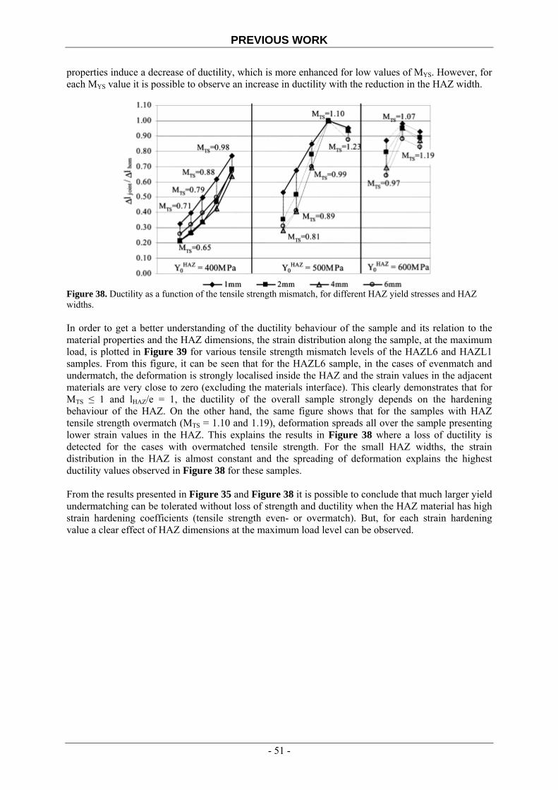
PREVIOUS WORK

properties induce a decrease of ductility, which is more enhanced for low values of MYS. However, for each MYS value it is possible to observe an increase in ductility with the reduction in the HAZ width.

Figure 38. Ductility as a function of the tensile strength mismatch, for different HAZ yield stresses and HAZ widths. In order to get a better understanding of the ductility behaviour of the sample and its relation to the material properties and the HAZ dimensions, the strain distribution along the sample, at the maximum load, is plotted in Figure 39 for various tensile strength mismatch levels of the HAZL6 and HAZL1 samples. From this figure, it can be seen that for the HAZL6 sample, in the cases of evenmatch and undermatch, the deformation is strongly localised inside the HAZ and the strain values in the adjacent materials are very close to zero (excluding the materials interface). This clearly demonstrates that for MTS ≤ 1 and lHAZ/e = 1, the ductility of the overall sample strongly depends on the hardening behaviour of the HAZ. On the other hand, the same figure shows that for the samples with HAZ tensile strength overmatch (MTS = 1.10 and 1.19), deformation spreads all over the sample presenting lower strain values in the HAZ. This explains the results in Figure 38 where a loss of ductility is detected for the cases with overmatched tensile strength. For the small HAZ widths, the strain distribution in the HAZ is almost constant and the spreading of deformation explains the highest ductility values observed in Figure 38 for these samples. From the results presented in Figure 35 and Figure 38 it is possible to conclude that much larger yield undermatching can be tolerated without loss of strength and ductility when the HAZ material has high strain hardening coefficients (tensile strength even- or overmatch). But, for each strain hardening value a clear effect of HAZ dimensions at the maximum load level can be observed.

- 51 -

PREVIOUS WORK

Figure 39. Strain distribution along the samples HAZL6 and HAZL1 for various tensile strength mismatch ratios.

5.3.3.2 Study of the influence of constraint in the plastic behaviour of the HAZ When a butt weld is loaded in tension normal to the weld direction, as soon as yielding occurs constraint is developed at the interface between the soft material and the adjacent materials that remain unyielded. This tends to prevent strain in the transverse direction and the soft material develops a hydrostatic stress component. Thus, relatively larger tensile stresses are required to further increase plastic strain in the soft material. It is possible to analyze the influence of constraint in the HAZ strength, calculating the strain energy absorbed in the HAZ material until the maximum load is attained in the sample. The plastic strain energy per unit volume is given by the equation: pεdσW ∫= (5.7)

Where σ is the equivalent stress and pε is the equivalent plastic strain. Due to constraint, it can be assumed that the resulting strain energy in the constrained HAZ (Wc) can be decomposed into two components: (5.8) hethomc WWW += Where Whom is the strain energy absorbed during the homogeneous deformation of a uniaxial tensile sample of the same material of the HAZ (this energy can be calculated knowing the mechanical properties of each HAZ material), and Whet is a term associated with the presence of constraint.

- 52 -

PREVIOUS WORK

Figure 40 and Figure 41 shows the ratio Whet/Whom, as a function of the hardening coefficient and HAZ width. This ratio can be considered as a constraint factor that expresses the nature and magnitude of the constraint effects in the plastic behaviour of the HAZ. In these figures, positive values of the constraint factor when the maximum load in the overall joint is attained, imply that Wc > Whom. In these cases, the hydrostatic stress tensor induced by constraint increases the material strength in the HAZ. Moreover, Figure 40 and Figure 41 shows in some cases negative values of the constraint factor, indicating that Wc < Whom. In these cases, the maximum load of the sample occurs in the adjacent regions and the equivalent stress and strain values in the HAZ are lower than the maximum strength of this material. This occurs for materials with overmatch tensile strength and also, in some cases of evenmatch and undermatch tensile strength.

5.3.3.3 Influence of the HAZ dimension in the constraint effect For various mismatch conditions, Figure 40 shows positive (HAZL1 sample) and negative (HAZL6 sample) values of the constraint factor, indicating a strong influence of the size of the HAZ in the constraint effects. This can be better understood by analyzing the equivalent stress and stress in the thickness and width directions (σYY = σZZ due to symmetry) plotted along a line in the HAZ of these samples. This is carried out in Figure 42, where the stress lines are plotted for different tensile displacements in samples with HAZ material (Y0

HAZ = 400 MPa, MTS = 0.65). The line with the highest stress levels corresponds to stress values at the maximum load. Comparing the stress lines plotted in each graph, it is possible to understand the differences in the plastic deformation behaviour observed in Figure 40.

Figure 40. Strain energy ratio as a fuction of the hardening coefficient (n) for various HAZ widths in the case of HAZ yield strength = 400 MPa For the sample HAZL1, positive stresses in the thickness direction constraint the deformation in the HAZ. This necking inhibition enhances the material strength resulting in a positive constraint factor. On the other hand, for the sample HAZL6, the stresses in the thickness directions are negative which leads to a decrease in the hydrostatic stress. The deformation in the thickness direction is now facilitated leading to premature necking in the HAZ and subsequent negative energy balance. In the case of Y0

HAZ = 500 and 600 MPa, the constraint factor for samples HAZL6 is now positive. This indicates that the negative effect of the constraint in strength for large HAZ widths vanishes with increasing yield strength in this region. In fact, for such high yield strength values, the stress distribution in the sample at the beginning of deformation is uniform, avoiding premature strain localisation in the HAZ.

- 53 -

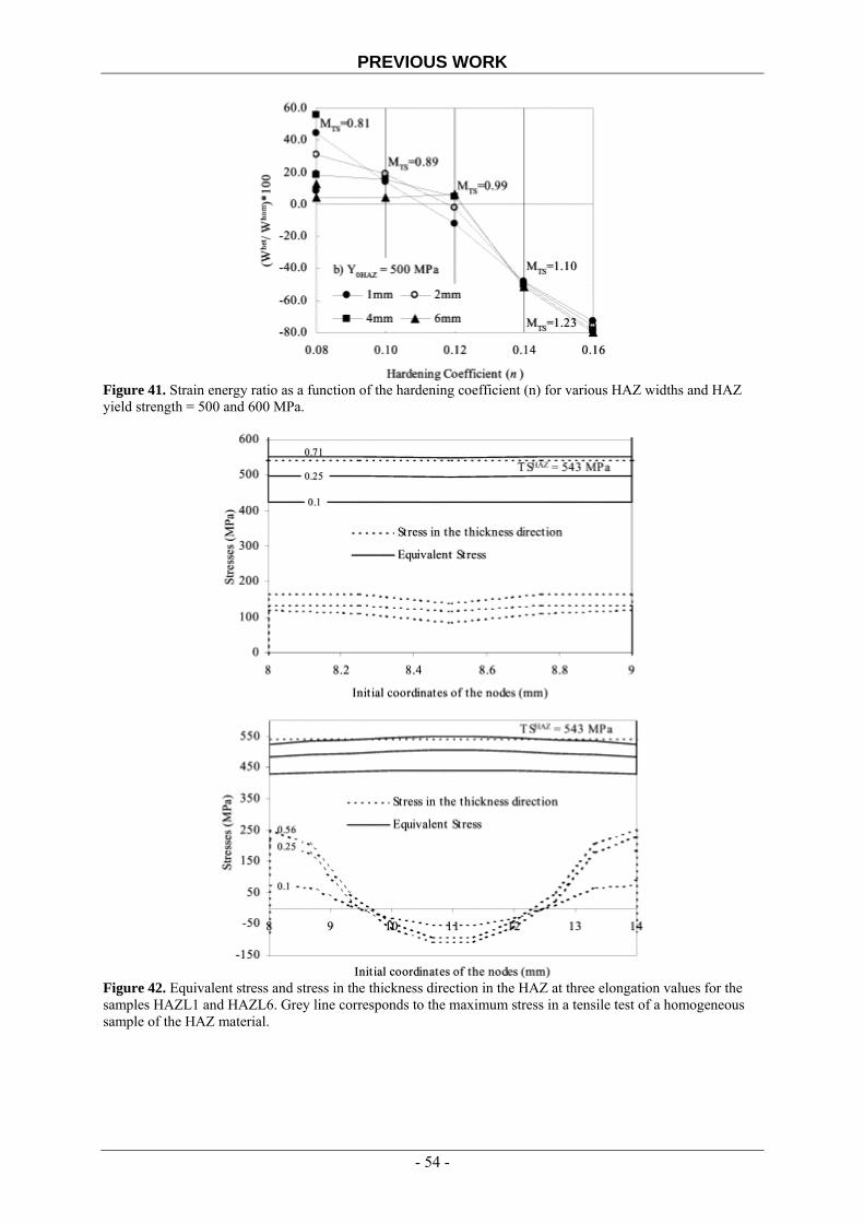
PREVIOUS WORK

Figure 41. Strain energy ratio as a function of the hardening coefficient (n) for various HAZ widths and HAZ yield strength = 500 and 600 MPa.

Figure 42. Equivalent stress and stress in the thickness direction in the HAZ at three elongation values for the samples HAZL1 and HAZL6. Grey line corresponds to the maximum stress in a tensile test of a homogeneous sample of the HAZ material.

- 54 -

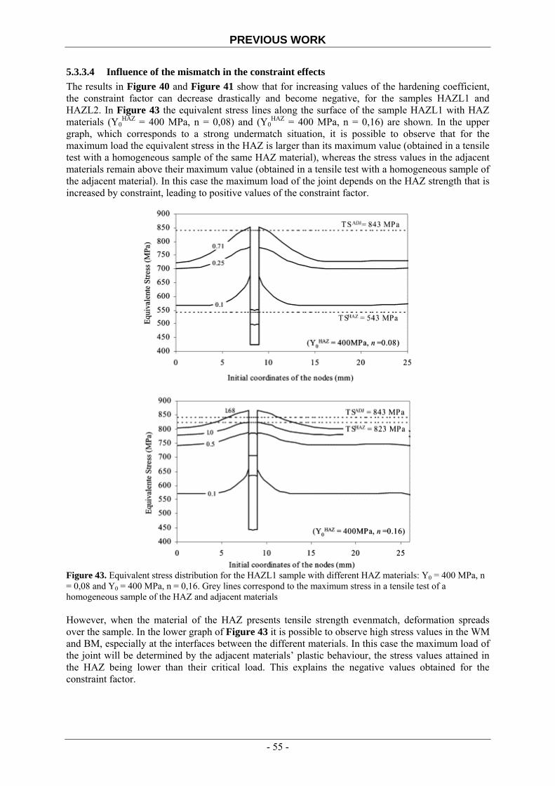
PREVIOUS WORK

5.3.3.4 Influence of the mismatch in the constraint effects The results in Figure 40 and Figure 41 show that for increasing values of the hardening coefficient, the constraint factor can decrease drastically and become negative, for the samples HAZL1 and HAZL2. In Figure 43 the equivalent stress lines along the surface of the sample HAZL1 with HAZ materials (Y0

HAZ = 400 MPa, n = 0,08) and (Y0HAZ = 400 MPa, n = 0,16) are shown. In the upper

graph, which corresponds to a strong undermatch situation, it is possible to observe that for the maximum load the equivalent stress in the HAZ is larger than its maximum value (obtained in a tensile test with a homogeneous sample of the same HAZ material), whereas the stress values in the adjacent materials remain above their maximum value (obtained in a tensile test with a homogeneous sample of the adjacent material). In this case the maximum load of the joint depends on the HAZ strength that is increased by constraint, leading to positive values of the constraint factor.

Figure 43. Equivalent stress distribution for the HAZL1 sample with different HAZ materials: Y0 = 400 MPa, n = 0,08 and Y0 = 400 MPa, n = 0,16. Grey lines correspond to the maximum stress in a tensile test of a homogeneous sample of the HAZ and adjacent materials However, when the material of the HAZ presents tensile strength evenmatch, deformation spreads over the sample. In the lower graph of Figure 43 it is possible to observe high stress values in the WM and BM, especially at the interfaces between the different materials. In this case the maximum load of the joint will be determined by the adjacent materials’ plastic behaviour, the stress values attained in the HAZ being lower than their critical load. This explains the negative values obtained for the constraint factor.

- 55 -

PREVIOUS WORK

5.3.4 Conclusions The first conclusions concern the overall strength and ductility of the joint in relation to mismatch and HAZ dimensions. From the results it is possible to conclude that:

• The tensile strength of the soft zone determines the overall strength of the joint. In fact, independent to the level of yield stress undermatch, the joints achieve the base plate strength in all tensile strength overmatch situations. For evenmatch and undermatch cases the strength of the joint is strongly dependent on the HAZ dimensions.

• For the cases in which the ratio width of the HAZ to sample thickness is less than 1/3, the loss of strength never exceeds 10%, even for cases of extreme strength undermatch. However, the joint strength decreases linearly with increasing HAZ widths.

• In almost all the cases, mismatch leads to a decrease in joint ductility, which varies depending on HAZ dimensions and hardening values.

In any case, the mechanical behaviour of the overall joint depends on the plastic distribution inside the HAZ. In fact, large tensile strength undermatch promotes strain localization in the HAZ from the start of deformation, but for very small HAZ dimensions (width < 1/3 of the thickness) the soft material can achieve the base plate strength. Depending on the tensile strength mismatch it can be stated that:

• In almost all the undermatch cases and for lHAZ/e rations lower than unity, an apparent increase in the material strength is observed due to constraint.

• For the tensile strength evenmatch situations, the HAZ constraint induces spreading of deformation to the adjacent materials avoiding deformation in the soft HAZ material.

• Finally, for large yield strength undermatch and HAZ widths equal to the sample thickness, constraint promotes premature failure in the soft zone decreasing the overall strength of the joint even more.

- 56 -

EXPERIMENTAL PROCEDURE

6 Laboratory tests

6.1 Aim and approach

The aim of the practical tests was to see how and if the static strength of joints varied with changing geometrical and material parameters. Three different parameters were chosen to be varied:

• Width- to thickness relation • Undermatching level • Relative thickness

To get distinct results, only one parameter was varied at a time, the rest were pin-pointed. 6.1.1 Width- to Thickness The idea with studying the effect of the relation between width and thickness was to see how triaxiality affected the static strength of the joint. The plate thickness was kept constant while 5 different specimen widths were produced. Two joints (number 1 & 2) were made from joint type 1 (see Figure 44). The two joints were fabricated the following way: Coupon type 1: Steel: WELDOX 1100 Thickness: 5,5 mm Groove angle: 50º Process: FCAW Electrode: Filarc PZ 6149 Heat input: Δt8/5 ≈ 10 s Width of specimen web: 6, 12, 24, 48 & 96 mm Number of specimens: 3 for each width Σ = 15 individual specimens 6.1.2 Undermatching To produce different yield strength undermatching levels, two different steels and two different electrodes were used. Here, the aim was to achieve obvious differences by using a strongly undermatching electrode in both steels. With the slight difference in yield strength between the steels it would also be possible to produce moderately undermatching welds of different levels. Another benefit using the different steel qualities would be to see if the tensile behaviour was different between a quenched and tempered steel (WELDOX 1100) and a quenched and low tempered steel (WELDOX 960), when welded undermatched. Joint number 3 was made from joint type 5 (Figure 44). In this joint the lowest strength steel was welded with the strongest available consumable:

- 57 -

EXPERIMENTAL PROCEDURE

Coupon type 2: Steel: WELDOX 960 Thickness: 6 mm Groove angle: 50º Process: FCAW Electrode: Filarc PZ 6149 Heat input: Δt8/5 ≈ 10 s Width of specimen web: 24 mm Number of specimens: 3 Σ = 3 individual specimens Joint number 4 was made from joint type 1 (see Figure 44). In this joint the highest strength steel was welded with a strongly undermatching consumable: Coupon type 3: Steel: WELDOX 1100 Thickness: 5,5 mm Groove angle: 50º Process: FCAW Electrode: Filarc PZ 6145 Heat input: Δt8/5 ≈ 10 s Width of specimen web: 24 mm Number of specimens: 3 Σ = 3 individual specimens Joint number 5 was made from joint type 5 (see Figure 44). In this joint the lowest strength steel was welded with a strongly undermatching consumable: Coupon type 4: Steel: WELDOX 960 Thickness: 6 mm Groove angle: 50º Process: FCAW Electrode: Filarc PZ 6145 Heat input: Δt8/5 ≈ 10 s Width of specimen web: 24 mm Number of specimens: 3 Σ = 3 individual specimens The specimens with the highest strength steel and the strongest available consumable was taken from the results from coupon type 1, which was made for studying the width- to thickness relation. In total 12 (4×3) separate specimens were produced to study the undermatching effect. 6.1.3 Relative thickness The relative thickness is defined as the ratio between the width of the weld and the thickness of the plate, Satoh and Toyoda (1975). Changing the relative thickness would also show the effect of triaxiality in the joint. To vary the relative thickness, the plate thickness was kept constant at 12 mm.

- 58 -

EXPERIMENTAL PROCEDURE

The width of the weld was changed by altering the groove angles. Three angles were chosen to be studied; 7, 50 and 80º. The three angles would give the following relative thicknesses: 7°: X = 0,1225 50º: X = 0,93 80°: X = 1,68 Unfortunately the 7° V-joint preparation was troublesome to weld practically. Therefore this joint type was discarded. In another attempt to achieve a small relative thickness, an x-type joint preparation was used. Two joints were welded with different welding parameters; none of the joints were defect-free according to the non-destructive testing (see section 6.2.6). Joint number 6 was made from joint type 3 (see Figure 44). In this joint the groove angle was set to 50°: Coupon type 5: Steel: WELDOX 1100 Thickness: 12 mm Groove angle: 50º Process: FCAW Electrode: Filarc PZ 6149 Heat input: Δt8/5 ≈ 10 s Width of specimen web: 24 mm Number of specimens: 3 Σ = 3 individual specimens Joint number 7 was made from joint type 4 (see Figure 44). In this joint the groove angle was set to 80°: Coupon type 6: Steel: WELDOX 1100 Thickness: 12 mm Groove angle: 80º Process: FCAW Electrode: Filarc PZ 6149 Heat input: Δt8/5 ≈ 10 s Width of specimen web: 24 mm Number of specimens: 3 Σ = 3 individual specimens 6.1.4 Number of specimens Altogether 30 different test specimens were fabricated. 6.2 Experimental Procedure

Welds were produced in coupon plates of high strength, quenched and tempered steel, (WELDOX 960 and WELDOX 1100) of various thicknesses. The coupon sides were milled to specific angles. The welding began after joint preparation. To avoid using defective material, all joint were radiographed. Tensile test specimens were extracted from the welded joints. Macro tests were also taken from all joints to decide hardness variations across the welds.

- 59 -

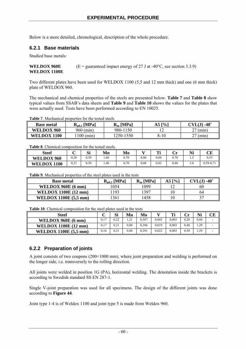
EXPERIMENTAL PROCEDURE

Below is a more detailed, chronological, description of the whole procedure. 6.2.1 Base materials Studied base metals: WELDOX 960E (E = guaranteed impact energy of 27 J at -40°C, see section 3.3.9) WELDOX 1100E Two different plates have been used for WELDOX 1100 (5,5 and 12 mm thick) and one (6 mm thick) plate of WELDOX 960. The mechanical and chemical properties of the steels are presented below. Table 7 and Table 8 show typical values from SSAB’s data sheets and Table 9 and Table 10 shows the values for the plates that were actually used. Tests have been performed according to EN 10025. Table 7. Mechanical properties for the tested steels

Base metal Rp0,2 [MPa] Rm [MPa] A5 [%] CVL(J) -40˚ WELDOX 960 960 (min) 980-1150 12 27 (min)

WELDOX 1100 1100 (min) 1250-1550 8-10 27 (min) Table 8. Chemical composition for the tested steels.

Steel C Si Mn Mo V Ti Cr Ni CE WELDOX 960 0,20 0,50 1,60 0,70 0,06 0,04 0,70 1,5 0,55

WELDOX 1100 0,21 0,50 1,40 0,70 0,08 0,02 0,80 3,0 0,59-0,71

Table 9. Mechanical properties of the steel plates used in the tests

Base metal Rp0,2 [MPa] Rm [MPa] A5 [%] CVL(J) -40˚ WELDOX 960E (6 mm) 1054 1099 12 60

WELDOX 1100E (12 mm) 1193 1397 10 64 WELDOX 1100E (5,5 mm) 1361 1458 10 37

Table 10. Chemical composition for the steel plates used in the tests

Steel C Si Mn Mo V Ti Cr Ni CE WELDOX 960E (6 mm) 0,17 0,22 1,21 0,587 0,043 0,003 0,20 0,04 -

WELDOX 1100E (12 mm) 0,17 0,21 0,88 0,386 0,019 0,003 0,48 1,29 -

WELDOX 1100E (5,5 mm) 0,16 0,21 0,88 0,391 0,022 0,003 0,50 1,29 -

6.2.2 Preparation of joints A joint consists of two coupons (200×1000 mm), where joint preparation and welding is performed on the longer side, i.e. transversely to the rolling direction. All joints were welded in position 1G (PA), horizontal welding. The denotation inside the brackets is according to Swedish standard SS EN 287-1. Single V-joint preparation was used for all specimens. The design of the different joints was done according to Figure 44. Joint type 1-4 is of Weldox 1100 and joint type 5 is made from Weldox 960.

- 60 -

EXPERIMENTAL PROCEDURE

Figure 44. Joint designs, single-V joint preparation 6.2.3 Welding processes The joints were welded with:

• Flux Cored Arc Welding (FCAW) ISO-6947 136 6.2.4 Electrodes Two different welding wires were used. One wire (PZ 6149) was the strongest available electrode on the market. The other wire was chosen to give a certain level of undermatch. Filarc PZ 6145 has a yield strength around 500-600 MPa. Both welding wires had a diameter of 1,2 mm. Table 11 Mechanical properties of the used welding wires according to Filarc’s data sheet

Welding wire Rp0,2 [MPa] Rm [MPa] A4 [%] CVL(J) -20˚ Filarc PZ6145 500 (min) 580-680 24 100 (min) Filarc PZ6149 890 (min) 950-1050 14 47 (min)

To study the correspondence between the strength of the electrode, given by the manufacturer, and the actual strength of the weld metal, static tension tests were performed on both weld metals. The testing was done slightly different to ISO and AWS standards, but can be compared to these without significant deviance.

50˚

7˚

12 mm 11 mm

4,5 mm

50˚

Joint type 1: 5,5 mm

Joint type 3:

12 mm 11 mm Joint type 4:

80˚

5,5 mm Joint type 2:

50˚

5 mm Joint type 5: 6 mm

- 61 -

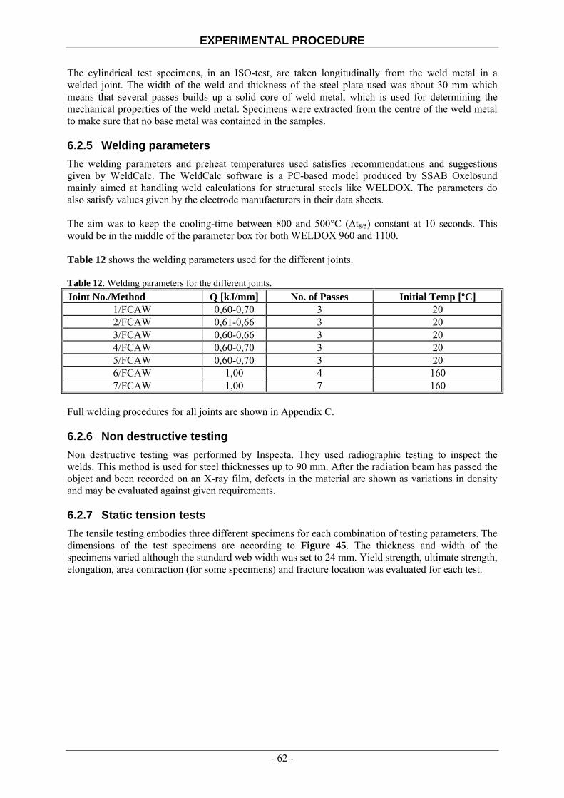
EXPERIMENTAL PROCEDURE

The cylindrical test specimens, in an ISO-test, are taken longitudinally from the weld metal in a welded joint. The width of the weld and thickness of the steel plate used was about 30 mm which means that several passes builds up a solid core of weld metal, which is used for determining the mechanical properties of the weld metal. Specimens were extracted from the centre of the weld metal to make sure that no base metal was contained in the samples. 6.2.5 Welding parameters The welding parameters and preheat temperatures used satisfies recommendations and suggestions given by WeldCalc. The WeldCalc software is a PC-based model produced by SSAB Oxelösund mainly aimed at handling weld calculations for structural steels like WELDOX. The parameters do also satisfy values given by the electrode manufacturers in their data sheets. The aim was to keep the cooling-time between 800 and 500°C (Δt8/5) constant at 10 seconds. This would be in the middle of the parameter box for both WELDOX 960 and 1100. Table 12 shows the welding parameters used for the different joints. Table 12. Welding parameters for the different joints. Joint No./Method Q [kJ/mm] No. of Passes Initial Temp [ºC]

1/FCAW 0,60-0,70 3 20 2/FCAW 0,61-0,66 3 20 3/FCAW 0,60-0,66 3 20 4/FCAW 0,60-0,70 3 20 5/FCAW 0,60-0,70 3 20 6/FCAW 1,00 4 160 7/FCAW 1,00 7 160

Full welding procedures for all joints are shown in Appendix C. 6.2.6 Non destructive testing Non destructive testing was performed by Inspecta. They used radiographic testing to inspect the welds. This method is used for steel thicknesses up to 90 mm. After the radiation beam has passed the object and been recorded on an X-ray film, defects in the material are shown as variations in density and may be evaluated against given requirements. 6.2.7 Static tension tests The tensile testing embodies three different specimens for each combination of testing parameters. The dimensions of the test specimens are according to Figure 45. The thickness and width of the specimens varied although the standard web width was set to 24 mm. Yield strength, ultimate strength, elongation, area contraction (for some specimens) and fracture location was evaluated for each test.

- 62 -

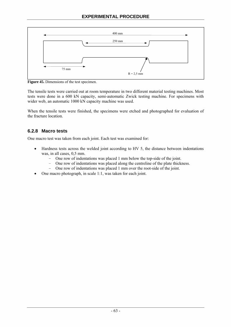
EXPERIMENTAL PROCEDURE

Figure 45. Dimensions of the test specimen.

250 mm

400 mm

75 mmR = 2,5 mm

The tensile tests were carried out at room temperature in two different material testing machines. Most tests were done in a 600 kN capacity, semi-automatic Zwick testing machine. For specimens with wider web, an automatic 1000 kN capacity machine was used. When the tensile tests were finished, the specimens were etched and photographed for evaluation of the fracture location. 6.2.8 Macro tests One macro test was taken from each joint. Each test was examined for:

• Hardness tests across the welded joint according to HV 5, the distance between indentations was, in all cases, 0,5 mm.

- One row of indentations was placed 1 mm below the top-side of the joint. - One row of indentations was placed along the centreline of the plate thickness. - One row of indentations was placed 1 mm over the root-side of the joint.

• One macro photograph, in scale 1:1, was taken for each joint.

- 63 -

RESULTS

7 Results

7.1 Mechanical tests of welded joints

Results from static tension tests of the welded joints are given in Table 13. The yield strength, ultimate strength, elongation and failure position has been evaluated in every specimen. Contraction was only evaluated towards the end of the test series. Table 13. Mechanical properties of the welded joints.

SPEC

IME

N#

STE

EL

PLA

TE

TH

ICK

NE

SS [MM

] JO

INT N

UM

BER

WITH

IN

BR

AC

KETS

WE

LD

ING

PRO

CE

SS

EL

EC

TR

OD

E

GR

OO

VE

AN

GL

E [°]

WID

TH

[MM

]

RP0,2 [M

PA]

RM [M

PA]

A5 [%

]

Z [%

]

POSIT

ION

OF FA

ILU

RE

8

1 960 6 FCAW PZ 6149 50 24 906,253 982,58 11 BM 2 960 6 FCAW PZ 6149 50 24 1047,03 1103,67 11 BM 3 960 6 FCAW PZ 6149 50 24 1004,12 1077 9 BM 4 1100 5,5 FCAW PZ 6145 50 24 775,144 915,705 6 WM 5 1100 5,5 FCAW PZ 6145 50 24 805,419 942,756 5 HAZ6 1100 5,5 FCAW PZ 6145 50 24 823,475 979,665 6 HAZ7 960 6 FCAW PZ 6145 50 24 805,082 931,619 3 WM 8 960 6 FCAW PZ 6145 50 24 827,83 934,952 5 WM 9 960 6 FCAW PZ 6145 50 24 820,137 921,05 4 WM

10 1100 5,5 (2) FCAW PZ 6149 50 12 1002,7 1108,39 6 WM 11 1100 5,5 (2) FCAW PZ 6149 50 12 1003,68 1115,98 5 BM 12 1100 5,5 (2) FCAW PZ 6149 50 12 968,408 1086,67 8 WM 13 1100 5,5 (2) FCAW PZ 6149 50 24 1069,16 1136,81 7 HAZ14 1100 5,5 (2) FCAW PZ 6149 50 24 1032,18 1128,15 8 HAZ15 1100 5,5 (2) FCAW PZ 6149 50 24 1031,57 1123,66 8 WM 16 1100 5,5 (2) FCAW PZ 6149 50 48 1108,12 1169,26 6 WM 17 1100 5,5 (2) FCAW PZ 6149 50 48 1105,03 1190,79 4 WM 18 1100 5,5 (2) FCAW PZ 6149 50 48 1142,87 1184,35 6 WM 19 1100 5,5 (2) FCAW PZ 6149 50 6 939,607 1063,48 9,3 WM 20 1100 5,5 (2) FCAW PZ 6149 50 6 967,265 1069,42 11,4 BM 21 1100 5,5 (2) FCAW PZ 6149 50 6 947,322 1075,32 12 BM 22 1100 5,5 (1) FCAW PZ 6149 50 96 1159 1193 3 HAZ23 1100 5,5 (1) FCAW PZ 6149 50 96 1148 1177 3 HAZ24 1100 5,5 (1) FCAW PZ 6149 50 96 1172 1205 3 BM 25 1100 12 FCAW PZ 6149 50 24 1012,79 1090,44 7 23 HAZ26 1100 12 FCAW PZ 6149 50 24 1071,53 1099,01 5 24 HAZ

8 BM = Base Metal, WM = Weld Metal, HAZ = Heat Affected Zone

- 64 -

RESULTS

27 1100 12 FCAW PZ 6149 50 24 992,255 1089,5 7 23 HAZ28 1100 12 FCAW PZ 6149 80 24 939,581 1031,16 7 23 HAZ29 1100 12 FCAW PZ 6149 80 24 834,008 1038,4 7 29 HAZ30 1100 12 FCAW PZ 6149 80 24 934,168 1030,46 6 22 HAZ 7.2 Mechanical tests on weld metals

The values in Table 14 correspond to measured values from three separate tests. The yield strength, ultimate strength and elongation have been evaluated for every specimen. Table 14. Mechanical properties of the weld metals - measured

Welding wire Rp0,2 [MPa] Rp0,2ave [MPa] Rm [MPa] Rm

ave [MPa] A5 [%] Filarc PZ6145 618, 491, 608 572 696, 688, 689 691 23, 21, 23 Filarc PZ6149 804, 844, 797 815 1001, 1015, 1028 1015 17, 17, 14

The observed ultimate strength is within the span that the manufacturer specifies. For PZ6145 the average ultimate strength is even above this range. The variation of the ultimate strength is only 8 MPa for PZ6145 and 27 MPa for PZ6149. The variation of the yield strength is greater (127 MPa for PZ6145 and 47 MPa for PZ6149). Also, the average yield strength of PZ6149 is lower than what was expected. Filarc prescribed a minimum yield strength of 890 MPa for this electrode. 7.3 Macro tests

Results from the macro-tests can be found in Appendix D. There are diagrams from hardness tests and macro-photos. Because of symmetry, only one side of the test sample was evaluated for Table 14. The values for the base metal and weld metal are average values over applicable lengths according to each test specification in section 7.3.1-7.3.6 below. Table 15. Hardness test according to HV 5, the distance between indentations was 0,5 mm. Test No.

Top BM

Top HAZmin

Top HAZmax

Top WM

Centre BM

Centre HAZmin

Centre HAZmax

Centre WM

Root BM

Root HAZmin

Root HAZmax

Root WM

1-1 458 315 449 355 449 314 437 361 465 310 465 351 1-2 453 318 437 369 439 315 432 362 464 307 454 334 2 352 332 410 373 346 323 384 344 350 303 356 344 3 441 314 406 245 427 282 369 237 434 252 365 235 4 346 307 382 247 343 303 356 240 348 287 356 234 5 420 302 398 368 423 290 398 353 422 276 400 326 6 416 304 402 378 414 280 402 326 410 265 396 289 The average hardness of the WELDOX 1100E plate with 5,5 mm thickness was 446HV5 which corresponds to an ultimate strength of 1338 MPa. The average hardness of the WELDOX 960E plate with 6 mm thickness was 348HV5 which corresponds to an ultimate strength of 1044 MPa. The average hardness of the WELDOX 1100E plate with 12 mm thickness was 418HV5 which corresponds to an ultimate strength of 1254 MPa. The average hardness of the Filarc PZ 6149 electrode was 347HV5 which corresponds to an ultimate strength of 1041 MPa.

- 65 -

RESULTS

The average hardness of the Filarc PZ 6145 electrode was 240HV5 which corresponds to an ultimate strength of 720 MPa. In the welds where the difference in hardness between the base- and weld metal is large, like for test number three and four, the weld metal and the zones of HAZ are more clearly visible in hardness diagrams. It is hard to discern different zones in other welds where the difference in hardness is small. 7.3.1 Test No.1-1 Three rows of indentations were laid; one 1 mm below the top surface, one 0,5 mm above the centre and one 1 mm above the root surface. The total measured length was 71,5 mm. The base metal was, from the diagram, estimated to go from 0-15 mm. The weld metal, in the three different rows, was measured to go between: Top: 32-41 mm Centre: 33-37 mm Root: 35-36 mm This implies that the heat affected zone was between: Top: 15-32 mm Centre: 15-33 mm Root: 15-35 mm 7.3.2 Test No.1-2 Three rows of indentations were laid; one 1 mm below the top surface, one 0,5 mm above the centre and one 1 mm above the root surface. The total measured length was 70,0 mm. The base metal was, from the diagram, estimated to go from 0-15 mm. The weld metal, in the three different rows, was measured to go between: Top: 30-39 mm Centre: 33,5-38,5 mm Root: 35,5-37,5 mm This implies that the heat affected zone was between: Top: 15-30 mm Centre: 15-33,5 mm Root: 15-35,5 mm 7.3.3 Test No.2 Three rows of indentations were laid; one 1 mm below the top surface, one 0,5 mm above the centre and one 1 mm above the root surface. The total measured length was 72 mm. The base metal was, from the diagram, estimated to go from 0-25 mm. The weld metal, in the three different rows, was measured to go between: Top: 32-39 mm Centre: 33-37,5 mm Root: 35,5-36,5 mm

- 66 -

RESULTS

This implies that the heat affected zone was between: Top: 25-32 mm Centre: 25-33 mm Root: 25-35,5 mm 7.3.4 Test No.3 Three rows of indentations were laid; one 1 mm below the top surface, one 0,5 mm above the centre and one 1 mm above the root surface. The total measured length was 72 mm. The base metal was, from the diagram, estimated to go from 0-25 mm. The weld metal, in the three different rows, was measured to go between: Top: 32,5-39,5 mm Centre: 32,5-37 mm Root: 33-37,5 mm This implies that the heat affected zone was between: Top: 25-32,5 mm Centre: 25-32,5 mm Root: 25-33 mm In this test, the weld metal was clearly visible as a horizontal line with a hardness somewhere around 250HV5. On the sides of the weld metal (in GCHAZ) are hardness-peaks in all three rows. This indicates the presence of martensite. At a distance of approximately 5 mm from the fusion boundary is a noticeable dip in the hardness. The dip is located in the normalized HAZ in which the temperature has been between 900-1075ºC. The decrease of hardness is around 50HV5 and may be motivated by fine-grained ferrite. 7.3.5 Test No.4 Three rows of indentations were laid; one 1 mm below the top surface, one 0,5 mm above the centre and one 1 mm above the root surface. The total measured length was 72 mm. The base metal was, from the diagram, estimated to go from 0-25 mm. The weld metal, in the three different rows, was measured to go between: Top: 33-39 mm Centre: 34-38,5 mm Root: 35,5-37 mm This implies that the heat affected zone was between: Top: 25-33 mm Centre: 25-34 mm Root: 25-35,5 mm In this test the weld metal is fairly well defined, the hardness in HAZ varies in the different rows. 7.3.6 Test No.5 Three rows of indentations were laid; one 1 mm below the top surface, one 0,5 mm above the centre and one 1 mm above the root surface. The total measured length was 68 mm.

- 67 -

RESULTS

The base metal was, from the diagram, estimated to go from 0-20 mm. The weld metal, in the three different rows, was measured to go between: Top: 27,5-41 mm Centre: 30-37 mm Root: 32-36 mm This implies that the heat affected zone was between: Top: 20-27,5 mm Centre: 20-30 mm Root: 20-32 mm The hardness in both the weld metal and HAZ is not well defined. 7.3.7 Test No.6 Three rows of indentations were laid; one 1 mm below the top surface, one 0,5 mm above the centre and one 1 mm above the root surface. The total measured length was 69 mm. The base metal was, from the diagram, estimated to go from 0-15 mm. The weld metal, in the three different rows, was measured to go between: Top: 23,5-43,5 mm Centre: 28-39,5 mm Root: 30-37,5 mm This implies that the heat affected zone was between: Top: 15-23,5 mm Centre: 15-28 mm Root: 15-30 mm The hardness in both the weld metal and HAZ is not well defined.

- 68 -

ANALYSIS AND DISCUSSION

8 Analysis and Discussion

8.1 Width- to thickness relation

The values presented in Table 16 are the average values from the three different specimens. Both the yield strength and ultimate strength increases with increasing specimen width, as expected. It is noteworthy that the ratio between yield and ultimate strength also increases with increasing width. A low yield- to tensile strength ratio indicates a more ductile failure, Dexter (1997). Since the relatively thin plates used in ships and bridges do not develop significant constraint through the thickness, the maximum constraint is that associated with a plate of infinite width in the direction transverse to the axial loading, Dexter (1997). This explains the increasing strength shown below. Table 16. Mechanical properties from specimens where the width- to thickness relation was studied Specimen width fy [MPa] fu [MPa] A5 [MPa] fy/fu Fracture Location 6 mm 951,4 1069,4 10,9 0,89 WM/BM/BM 12 mm 991,6 1103,7 6,3 0,90 WM/BM/WM 24 mm 1044,3 1126,6 7,7 0,93 HAZ/HAZ/WM 48 mm 1118,7 1181,5 5,3 0,95 WM/WM/WM 96 mm 1159,7 1191,7 3 0,97 HAZ/HAZ/HAZ The yield strength of the base metal is, according to Table 9, 1361 MPa and the ultimate strength 1458 MPa. This results in a Y/T-ratio of 0,93. Also, the elongation seems to decrease with increasing specimen width.

Relative width

700

800

900

1000

1100

1200

1300

0 0,1 0,2 0,3 0,4 0,5 0,6 0,7 0,8 0,9 1

t/W

Stre

ss [M

Pa]

Yield strengthUltimate strength

Figure 46. Effect of width- to thickness relation on the strength of welded joints

- 69 -

ANALYSIS AND DISCUSSION

Both the yield- and ultimate strengths are plotted against the relative width in Figure 46, note the resemblance with Figure 20 b. 8.2 Undermatching

The values in Table 17 are the average of the three individual specimens tested for each set of parameters. The strength of the joints welded with the strongly undermatching wire is well above the strength of the wire, which is 691 MPa (PZ6145). This shows the effect of triaxiality and strain hardening. All undermatching levels are lower than what was anticipated. No welds were accomplished that were moderately (10-15%) undermatched. It is harder to evaluate the yield strength compared to the ultimate strength, which is noticeable in the larger variation of yield strength values for the weld metal. Therefore, undermatching indexes can vary with the way testing was done etc. The ratio between the joint strength and the base metal strength indicates how close the joint came to achieving the base metal’s strength. The fracture location in the joints of Weldox 960 steel and PZ6149 electrode shows that the global strength of the joint is governed by the base plate strength. On the other hand, when the same steel plate was welded with the weaker electrode all samples failed in the weld metal. Table 17. Mechanical properties from specimens where the undermatching effect was studied.

M = fyWM/fy

BM M = fu

WM/fuBMSteel/Electrode fy fu fy/fu A5

Fracture-Location fu

joint/fuBM

Typ.9 Obs.10 Obs

960/6149 985,8 1054,4 0,93 10,3 BM/BM/BM 1054/1094 = 0,96

890/1054 = 0,84

815/1054 = 0,77

1015/1099=0,92

1100/6145 801,3 946,0 0,85 5,7 WM/HAZ/HAZ 946/1458 = 0,65

500/1361 = 0,37

572/1361 = 0,42

691/1458 =0,47

960/6145 817,7 929,2 0,88 4,0 WM/WM/WM 929/1094 = 0,85

500/1054 = 0,47

572/1054 = 0,54

691/1099 =0,63

1100/6149 1044,3 1126,6 0,93 7,7 HAZ/HAZ/WM 1127/1458 = 0,77

890/1361 = 0,65

815/1361 = 0,60

1015/1458=0,70

Since the grade of yield strength undermatching is above 10-15 % a concentration of plastic flow should be provoked in the weakest zone, Dexter (1997). This implies a loss of strength and ductility. For the test series with Weldox 1100/PZ6145, the weakest zone seems to be the HAZ. For the test series with Weldox 960/PZ6145, the weakest zone is the weld metal. And for the test series with Weldox 1100/PZ6149 the weakest zone, again, seems to be the HAZ. For the test series with Weldox 960/PZ6149 all fractures was located in the base metal. This means that the joint achieved the base plate’s strength and ductility in spite of the low grade of undermatching. 8.3 Relative thickness

The values in Table 18 are the average of the three individual specimens tested for each set of parameters.

9 Typical values from the manufactor 10 Measured values from our test series

- 70 -

ANALYSIS AND DISCUSSION

As mentioned in section 6.1.3 there was some problems to fabricate specimens with a low relative thickness (7º groove angle). One way to go would be to use the Rapid Processing method to get a small weld metal volume, but it was not possible to weld that small groove angles even with this method. Table 18. Mechanical properties of specimens where the effect of relative thickness was studied. Groove Angle [º] Relative Thickness fy fu A5 fy/fu Fracture-Location

50 0,93 1025,5 1093,0 6,3 0,94 HAZ/HAZ/HAZ 80 1,68 902,6 1033,3 6,7 0,87 HAZ/HAZ/HAZ

As expected the strength decreases with increasing relative thickness. In almost all the undermatch cases and for H0/t0 rations lower than unity, an apparent increase in the material strength is observed due to constraint, Fernandes et al. (2004). 8.4 Discussion

The ambition, from the start of this project, was to use two different welding techniques. One would be the conventional FCAW, which often is used in workshops when welding this kind of steel. The other one was thought to be the newer, low heat input, method Rapid Processing. With this method it would be possible to accomplish low heat input and less weld metal volume. It would also be interesting to see how this new method worked with these high strength steels. Unfortunately time and material ran out. This means that all welds are welded with FCAW and approximately the same heat input. It is definitely possible, for the global strength of an undermatched test specimen to achieve the base plate strength. For example specimens made from Weldox 960 steel and PZ6149 weld metal. All three of these specimens failed in the base metal although the observed undermatching index was as low as 77 %. Other sources (Dexter 1997) claims that the maximum tolerable undermatch is about 10-15 %. Under this level, plastic flow is induces in the weakest zone which reduces strength and ductility of the joint. We never managed to achieve the base plate strength in Weldox 1100 steel even though the electrode used was the strongest available on the market. These specimens failed in HAZ and had a matching index of 0,60. This means that it would be hard to reach the base plate strength for even higher strength steels (Weldox 1300) loaded in pure tension. If the thickness of the steel plate is kept constant and only the specimen width is increased, the global strength of the joint increases with the width of the specimens. Both the yield strength and ultimate strength increased with the specimen width, but the difference between them got smaller. This is due to constraint. When the soft weld starts to deform, the adjacent, unyielded base plate, constrains this deformation. The weld develops tension in the width-, thickness- and longitudinal directions. When the weld experiences tension in two or three material directions, the mean stress or hydrostatic stress in the weld is increased. Yielding of a material is governed by the Von-Mises Yield Criterion. Therefore, as the hydrostatic stress is increased by constraint, the magnitudes of the deviatoric stresses, which govern yielding, are reduced. Thus because of constraint, larger stresses are required to further increase plastic strain. The ductility of the joint seems to decrease with a decreasing undermatching index. According to Table 17 the elongation was 10,3 % at an undermatching index of 77 %. As mentioned before the failure is located in the base plate and the plastic flow is not only concentrated to the weakest zone but is spread out over a larger area. The elongation was only 4 % when the undermatching index was 54 %. All of these specimens failed in the weld metal.

- 71 -

ANALYSIS AND DISCUSSION

From the tests that were performed it is not possible to tell if the ductility increased with a reducing relative thickness. Both test series reached an elongation of about 6,5 % (see Table 18), and all specimens failed in HAZ. If a smaller relative thickness could have been achieved, the fracture could have been moved to the base plate, resulting in larger ductility. There is not enough test series to say whether there are any differences in the joint performances of quenched and tempered (Weldox 1100) and quenched and low tempered (Weldox 960) steel. To be able to evaluate that, joints in both steel types needs to have been equally undermatched and welded with the same parameters. In Table 17 there are two test series that have an undermatching index close to each other; Weldox 960/PZ6145 with M = 0,54 and Weldox 1100/PZ6149 with M = 0,60. If these two series are compared it is obvious that all joints in the quenched and low tempered steel failed in the weld metal and that joints in the quenched and tempered steel failed in HAZ. The Y/T-ratio of joints in Weldox 960 is lower together with the elongation. 8.5 Possible Sources of Error

There is always a risk that the statistical population is not big enough and that the observed behaviour is not representative. There could have been more test samples per varied parameter –three is maybe too few? The welding conditions used when testing the strength of the weld metal were not the same that were used for the rest of the welding. It was not possible to use these parameters due to the large weld metal volume in the weld metal tests. Also the strength of the weld metal does not take into consideration the “mixing effect” that occurs when welding joints of normal dimensions. The idea with the weld metal test is to test the weld metal only. The welding parameters were chosen so that they could be kept constant ((Δt8/5=10s). This compromised the welding result a bit. There were some problems with root cracks, but these should have been avoided with the help of non-destructive testing. The relative thickness is hard to define in a single V-joint preparation. In this paper the width of the weld metal is the width between the top-sides of the joint, including the root opening. There is always a risk of human error in fabrication or evaluation. It is difficult to evaluate the yield strength of the weld metal. The yield strength varied quite a lot, this influences the undermatching index. 8.6 Future Work

It would be interesting to do wide plate tests in a high capacity tensile testing machine to make the tests more realistic. If the width of the specimen is equal to the width of a flange in a bridge beam, constraint should really help to increase the strength. Even higher strength steel could be used; maybe Weldox 1300. It is probably hard to reach the base plate strength, but the joint would most likely be stronger than the weld metal. How close to the base metal strength is it possible to come? Other high strength steel types could be used. Not only quenched and tempered steels, but maybe TMCP? Try other parameters, not only geometric; for example heat input. Try other welding methods? It would still be interesting to use Rapid Processing as a low heat input method.

- 72 -

ANALYSIS AND DISCUSSION

Parallel to this work, an FEM-model has been created to study this phenomenon. The simulation was done by Mikael Möller at Uddcomb Engineering AB.

- 73 -

REFERENCES

9 References

[1] Ahlenius, E., Collin, P., Hedin, J. (1995). Att konstruera med höghållfast stål, publ. nr. 148, Stålbyggnadsintitutet, ISBN 91-7127-011-6

[2] AWS (American Welding Society) – Homepage. (2007-04-16). http://www.aws.org/w/a/

[3] Bakshi, O.A., Erofeev, V.V., Shakhmatov, M.V., Yaroslatsev, S.I., Anisimov, Yu.I. (1983).

Effect of the degree of mechanical heterogeneity on the static strength of welded joints, Welding Production, vol.30, no.4, Apr.1983, pp. 5-8

[4] Bang, K.S., Kim, W.Y. (2002). Estimation and prediction of HAZ softening in

thermomechanically controlled – rolled and accelerated – cooled steel, Welding journal, vol.81, no.8, pp. 174s-179s

[5] Bergh, S. (1987). Stål och svetsning, 4:e uppl., Kungl. tekniska högskolan, Avd. för

stålbyggnad, pp. 9-24

[6] Blomqvist, A. (1995). Mismatch in High Strength Steel Weldments, Application Research and Development, SSAB Oxelösund

[7] Blomqvist, A., Collin, P., Ranby A. (1996). Dimensionering av svetsförband i seghärdade

konstruktionsstål av Weldox 500 och Weldox 700, publ. nr. 156, Stålbyggnadsinstitutet, ISBN 91-7127-014-0

[8] Coe, F.R. (1973). Welding steels without hydrogen cracking, The Welding Institute

[9] Dawes, M.G. (1996). An introduction to K, CTOD and J fracture mechanics analysis and

toughness, and the application of these to metal structures, TWI Ref.. 7218.01/96/784.03

[10] Denys, R. (1994). Strength and performance characteristics of welded joints, ESIS 17, Mechanical Engineering Publications, London, pp. 59-102

[11] Dexter, R.J. (1997). Significance of strength undermatching of welds in structural behaviour,

GKSS Research Center Publications, Geesthacht, FRG, pp. 55-73

[12] Easterling, K. (1992). Introduction to the Physical Metallurgy of Welding, second edition, Butterworth-Heinemann Ltd., ISBN 0 7506 0394 1

[13] El-Shennawy, M., Minami, F., Toyoda, M., Kajimoto, K., Fujii, M., Murai, R. (1995).

Constraint effect in mis-matching and its application to KIC –measurement, 14th International Conference on Offshore Mechanics and Arctic Engineering, OMAE 95, Copenhagen, June 18-22

[14] Eriksson, K. (1989). Svetsteknologisk ABC, Institutionen för Svetsteknologi, KTH

[15] Eriksson, K. (2005). Att konstruera med stål – Modul 9, Brottmekanik,

Stålbyggnadsinstitutet, Luleå Tekniska Universitet, Kungliga Tekniska Högskolan

[16] Ersson, N. (2004). Dimensionering av kälsvetsar, Master’s thesis, Luleå University of Technology, Luleå, ISSN: 1402-1617

- 74 -

REFERENCES

[17] Fernandes, J.V., Loureiro, A, Menezes, L.F., Rodrigues, D.M. (2004). Numerical study of the

plastic behaviour in tension of welds in high strength steels, International Journal of Plasticity 20, pp. 1-18

[18] Fisher, J.W., Dexter, R.J. (1993). High performance steel bridges for the next century,

International Symposium on Low-Carbon Steels for the 90’s

[19] Gurev, A.V., Barmutov, V.P., Zhesin, Yu.D., Boikov, L.V. (1971). Calculated static tensile strength of composite specimens with soft interlayers, Volgograd Polytechnical Institute, translated from Problemy Prochnosti, no.1, pp. 9-13, January 1973

[20] Hamada, M. (2003). Control of strength and toughness at the heat affected zone, Welding

International, vol.17, no.4, pp.265-270

[21] Hannerz, N-E. (xxxx). Svetsningens materialteknologi, Kungliga Tekniska Högskolan, Institutionen för svetsteknologi, pp. 124-129

[22] Hertzberg, R. (1983). Deformation and fracture mechanics of engineering materials, Wiley,

ISBN 0-471-08609-6

[23] International Association for Bridge and Structural Engineering (IABSE). (2005). Use and application of high-performance steels for steel structures, ISBN 3-85748-113-7

[24] ISO (International Organization for Standardization). (2001). Destructive tests on welds in

metallic materials – Longitudinal tensile test on weld metal in fusion welded joints. ISO 5178:2001(E)

[25] Key to Steel (2007). True Stress – True Strain Curve, Key to Steel – The Worlds Most

Comprehensive Steel Database, URL: http://www.key-to-steel.com/Articles/Art42.htm (Read 2007-05-10)

[26] Loureiro, A.J.R. (2002). Effect of heat input on plastic deformation of undermatched welds,

Journal of Materials Processing Technology 128, pp. 240-249

[27] Lundqvist, B. (1980). Sandvikens handbok, svetsning, Sandvik AB, Sandvik publikation S-0,34-SWE

[28] Minami, F., Toyoda, M., Thaulow, C., Hauge, M. (1994). Effect of strength mis-match on

fracture mechanical behaviour of HAZ-nothched weld joint, Proceedings of the intermediate meeting of IIW Sub-Commission X-F, 28-29 April 1994, Paris, paper 8

[29] Ostsemin, A.A. (1990). Stress state and the static strength of mechanically inhomogeneous

welded joints. Report 2. Effect of a small degree of mechanical inhomogeneity on the strength of butt welded joints, Chelyabinsk Polytechnical Institute, translated from Problemy Prochnosti, no.4, pp. 35-38, April 1991

[30] Ostsemin, A.A., Dilman, V.L. (2005). Static strength and stressed state of mechanically

inhomogeneous butt welded joints with X-shape groove, Paton Welding Journal, no.11, Nov.2005, pp. 15-18

[31] Pisarski, H.G. (1996). Update on fracture toughness test methods for welded joints, TWI Ref.

7161.01/94/800

- 75 -

REFERENCES

[32] Pisarski, H.G., Dolby, R.E. (2003). The significance of softened HAZ’s in high strength structural steels, Welding in the World, vol.47, no.5-6, pp. 32-40

[33] Pisarski, H.G., Harrison, P.L. (2002). An investigation into the effect of weld strength

mismatch on the assessment of HAZ fracture toughness, EMAS Publications, vol.2, ISBN 1-901537-37-4, pp. 677-686

[34] Qiu, H., Mori, H., Enoki, M., Kishi, T. (2001). Effect of welding thermal cycle and cold

working on th eductility of SN490 steel under low and high-speed loading, Materials Science and Engineering, A316, pp. 217-223

[35] Satoh, K., Toyoda, M. (1975). Joint strength of heavy plates with lower strength weld metal,

Welding Research supplement, pp. 311-319

[36] SIS (Standardiseringen I Sverige). (1997). Welding consumables – Test methods – Part 1: Test piece for all weld metal test specimens in steel, nickel and nickel alloys. SS EN 1597-1:1997

[37] Svetskommissionen. (2007-04-16). http://www.svets.se/

[38] Thaulow, C., Toyoda, M. (1996). Strength mis-match effect on fracture behaviour of HAZ,

Second International Symposium on Mis-matching of Welds, Lüneburg, Germany, 24-26 April 1996

[39] Thelning, K-E. (1985). Stål och värmebehandling, andra utgåvan, Karlebo, ISBN 91-21-

13631-9

[40] Toyoda, M., Mochizuki, M., An, G.B., Ohmura, T. (2000). Characteristics of strength and fracture in undermatched welded joints by dynamic loading, Osaka University, Japan, IIW Doc. X-1459-2000

[41] TWI (The Welding Institute) – Materials Joining Technology Home Page. (2007-04-16).

http://www.twi.co.uk/j32k/index.xtp

[42] Umekuni, A., Masubuchi, K. (1997). Usefulness of undermatched welds for high-strength steels, Welding Journal, vol.76, no.7, pp. 256s-263s

[43] Weman, K. (2002). Svetshandbok, andra utgåvan, Karlebo, ISBN 91-47-05143-4

[44] Yue, J.J. (1997). Energy Concept for Fracture, Virginia Tech, URL:

http://www.sv.vt.edu/classes/MSE2094_NoteBook/97ClassProj/anal/yue/energy.html (Read 2007-05-09)

- 76 -

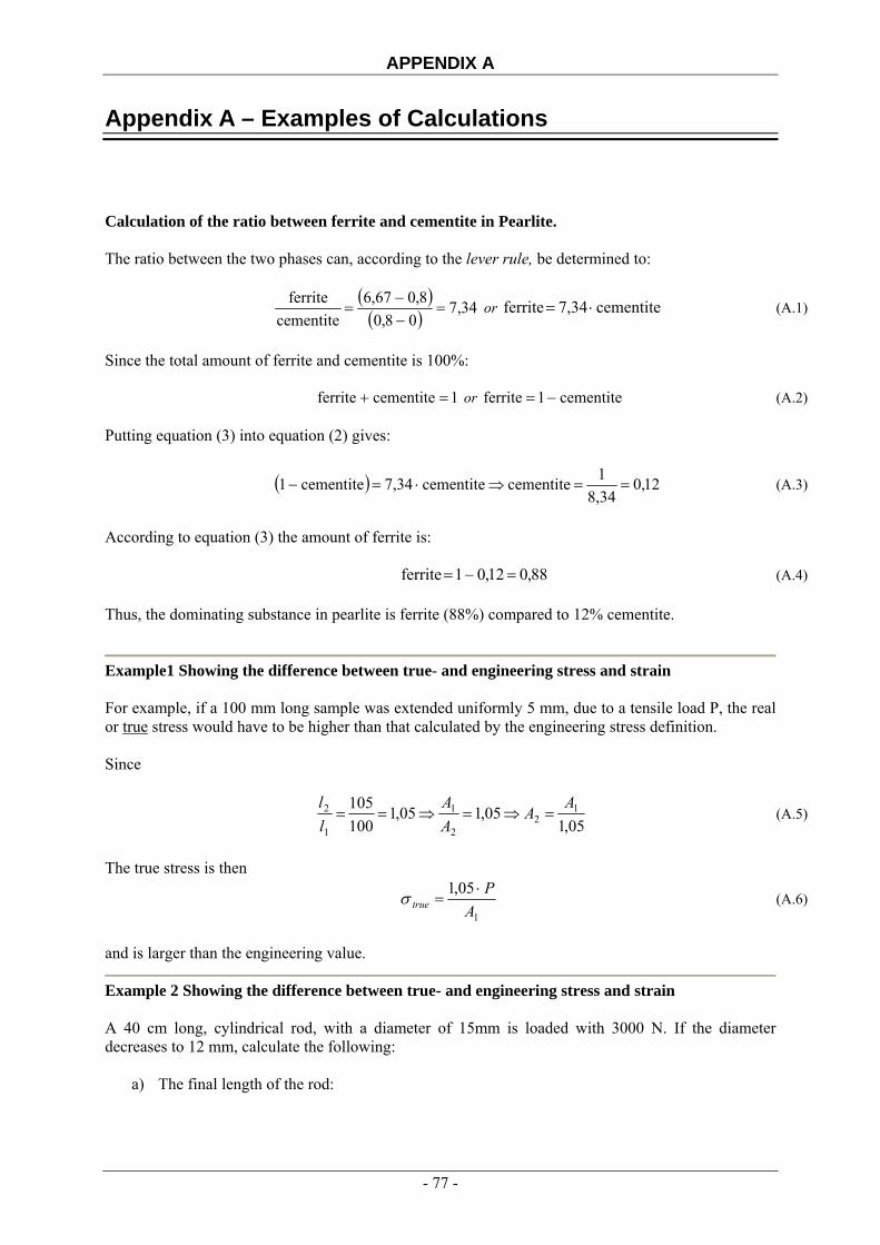
APPENDIX A

Appendix A – Examples of Calculations

Calculation of the ratio between ferrite and cementite in Pearlite. The ratio between the two phases can, according to the lever rule, be determined to:

( )( ) 34,7

08,08,067,6

cementiteferrite

=−−

= or cementite7,34ferrite ⋅= (A.1)

Since the total amount of ferrite and cementite is 100%: 1cementiteferrite =+ or cementite1ferrite −= (A.2) Putting equation (3) into equation (2) gives:

( ) 12,08,34

1cementitecementite7,34cementite1 ==⇒⋅=− (A.3)

According to equation (3) the amount of ferrite is: 88,012,01ferrite =−= (A.4) Thus, the dominating substance in pearlite is ferrite (88%) compared to 12% cementite.

Example1 Showing the difference between true- and engineering stress and strain For example, if a 100 mm long sample was extended uniformly 5 mm, due to a tensile load P, the real or true stress would have to be higher than that calculated by the engineering stress definition. Since

05,1

05,105,1100105 1

22

1

1

2 AA

AA

ll

=⇒=⇒== (A.5)

The true stress is then

1

05,1A

Ptrue

⋅=σ (A.6)

and is larger than the engineering value.

Example 2 Showing the difference between true- and engineering stress and strain A 40 cm long, cylindrical rod, with a diameter of 15mm is loaded with 3000 N. If the diameter decreases to 12 mm, calculate the following:

a) The final length of the rod:

- 77 -

APPENDIX A

( )

( )625

124

400154A

2

2

22

112211 =

⋅==

⋅⇒⋅=⋅

π

π

lA

llAlA [mm] (A.7)

b) The true stress and true strain at this load:

( )

5,261012

4

300023=

⋅⋅==

−πσ

itrue A

P[MPa] (A.8)

446,0400625lnln

0===

ll f

trueε or 44,6 % (A.9)

c) The engineering stress and strain at this load:

( )

0,171015

4

3000230=

⋅⋅==

−πσ

AP

eng [MPa] (A.10)

563,0400

400625

0

0 =−

=−

=l

ll fengε or 56,3 % (A.11)

- 78 -

APPENDIX B

Appendix B – Stress-Strain Plots

Specimen# 1-3, WX960, t = 6mm, FCAW, PZ 6149, w = 24mm

0

200

400

600

800

1000

1200

0,00 1,00 2,00 3,00 4,00 5,00 6,00 7,00 8,00

Strain [%]

Stre

ss [M

Pa]

Specimen1Specimen2Specimen3

Specimen# 4-6, WX110, t = 5.5mm, FCAW, PZ 6145, w = 24mm

0,00

200,00

400,00

600,00

800,00

1000,00

1200,00

0,00 1,00 2,00 3,00 4,00 5,00 6,00 7,00 8,00

Strain [%]

Stre

ss [M

Pa]

Specimen4Specimen5Specimen6

- 79 -

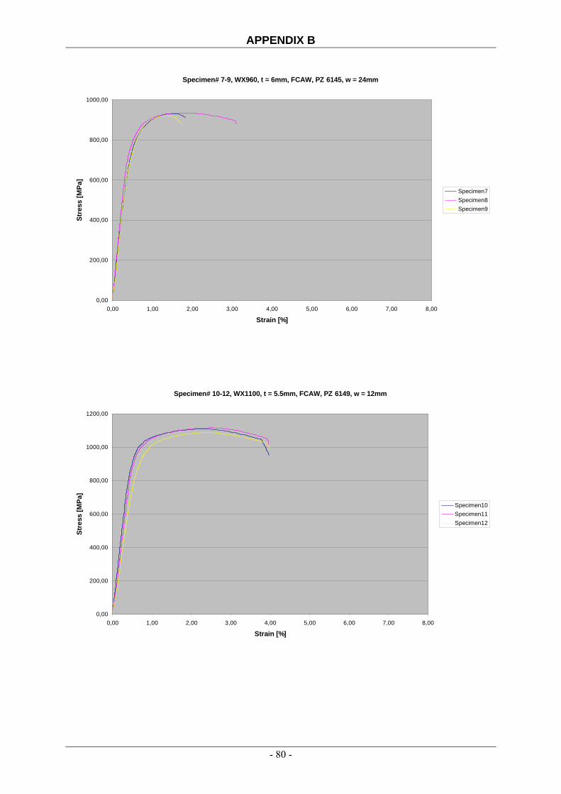
APPENDIX B

Specimen# 7-9, WX960, t = 6mm, FCAW, PZ 6145, w = 24mm

0,00

200,00

400,00

600,00

800,00

1000,00

0,00 1,00 2,00 3,00 4,00 5,00 6,00 7,00 8,00

Strain [%]

Stre

ss [M

Pa]

Specimen7Specimen8Specimen9

Specimen# 10-12, WX1100, t = 5.5mm, FCAW, PZ 6149, w = 12mm

0,00

200,00

400,00

600,00

800,00

1000,00

1200,00

0,00 1,00 2,00 3,00 4,00 5,00 6,00 7,00 8,00

Strain [%]

Stre

ss [M

Pa]

Specimen10Specimen11Specimen12

- 80 -

APPENDIX B

Specimen# 13-15, WX1100, t = 5.5mm, FCAW, PZ 6149, w = 24mm

0,00

200,00

400,00

600,00

800,00

1000,00

1200,00

0,00 1,00 2,00 3,00 4,00 5,00 6,00 7,00 8,00

Strain [%]

Stre

ss [M

Pa]

Specimen13Specimen14Specimen15

Specimen# 16-18, WX1100, t = 5.5mm, FCAW, PZ 6149, w = 48mm

0,00

200,00

400,00

600,00

800,00

1000,00

1200,00

1400,00

0,00 1,00 2,00 3,00 4,00 5,00 6,00 7,00 8,00

Strain [%]

Stre

ss [M

Pa]

Specimen16Specimen17Specimen18

- 81 -

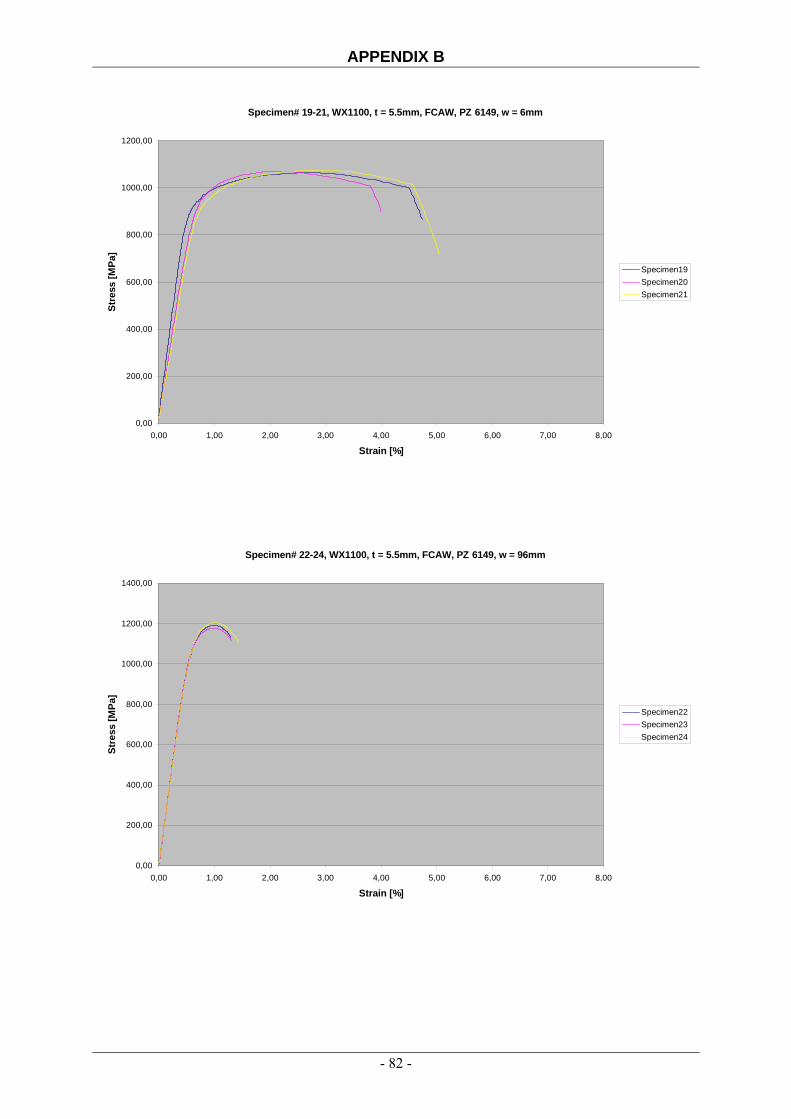
APPENDIX B

Specimen# 19-21, WX1100, t = 5.5mm, FCAW, PZ 6149, w = 6mm

0,00

200,00

400,00

600,00

800,00

1000,00

1200,00

0,00 1,00 2,00 3,00 4,00 5,00 6,00 7,00 8,00

Strain [%]

Stre

ss [M

Pa]

Specimen19Specimen20Specimen21

Specimen# 22-24, WX1100, t = 5.5mm, FCAW, PZ 6149, w = 96mm

0,00

200,00

400,00

600,00

800,00

1000,00

1200,00

1400,00

0,00 1,00 2,00 3,00 4,00 5,00 6,00 7,00 8,00

Strain [%]

Stre

ss [M

Pa]

Specimen22Specimen23Specimen24

- 82 -

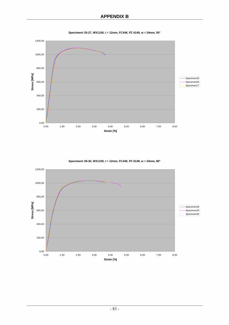
APPENDIX B

Specimen# 25-27, WX1100, t = 12mm, FCAW, PZ 6149, w = 24mm, 50°

0,00

200,00

400,00

600,00

800,00

1000,00

1200,00

0,00 1,00 2,00 3,00 4,00 5,00 6,00 7,00 8,00

Strain [%]

Stre

ss [M

Pa]

Specimen25Specimen26Specimen27

Specimen# 28-30, WX1100, t = 12mm, FCAW, PZ 6149, w = 24mm, 80°

0,00

200,00

400,00

600,00

800,00

1000,00

1200,00

0,00 1,00 2,00 3,00 4,00 5,00 6,00 7,00 8,00

Strain [%]

Stre

ss [M

Pa]

Specimen28Specimen29Specimen30

- 83 -

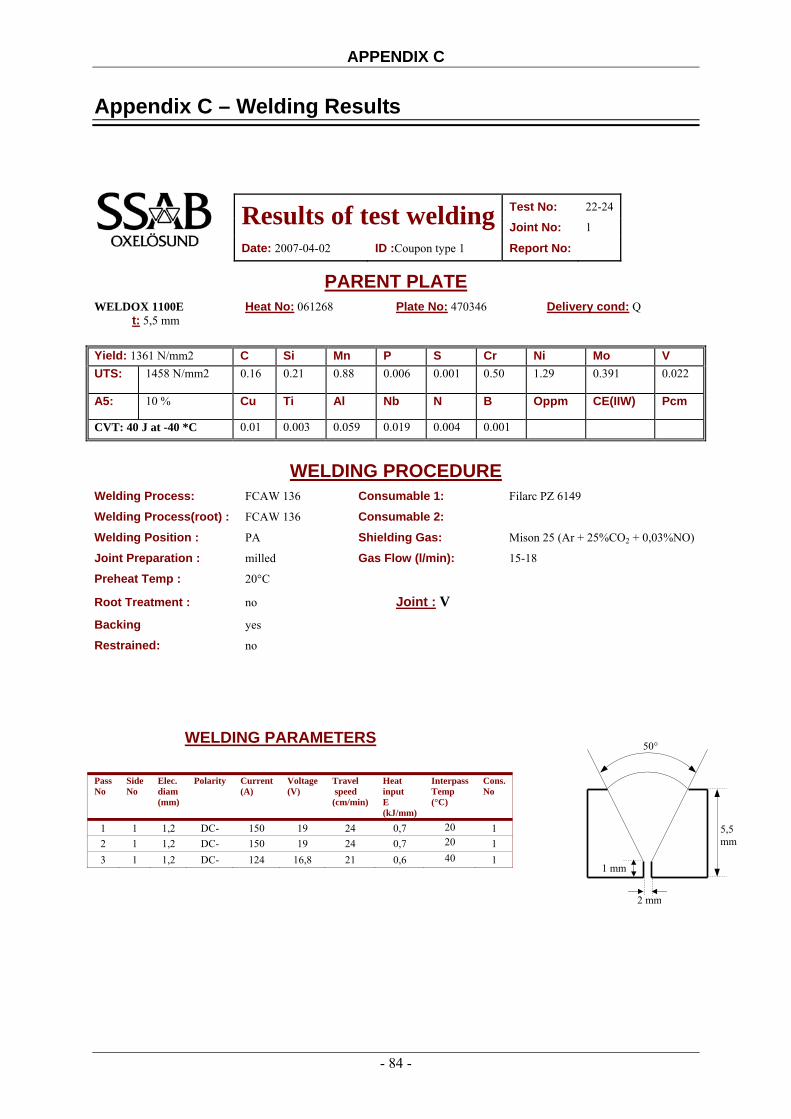
APPENDIX C

Appendix C – Welding Results

Test No: 22-24 Results of test welding Joint No: 1

Date: 2007-04-02 ID :Coupon type 1 Report No:

PARENT PLATE WELDOX 1100E Heat No: 061268 Plate No: 470346 Delivery cond: Q t: 5,5 mm Yield: 1361 N/mm2 C Si Mn P S Cr Ni Mo V UTS: 1458 N/mm2 0.16 0.21 0.88 0.006 0.001 0.50 1.29 0.391 0.022

A5: 10 % Cu Ti Al Nb N B Oppm CE(IIW) Pcm

CVT: 40 J at -40 *C 0.01 0.003 0.059 0.019 0.004 0.001

WELDING PROCEDURE

Welding Process: FCAW 136 Consumable 1: Filarc PZ 6149

Welding Process(root) : FCAW 136 Consumable 2:

Welding Position : PA Shielding Gas: Mison 25 (Ar + 25%CO2 + 0,03%NO)

Joint Preparation : milled Gas Flow (l/min): 15-18

Preheat Temp : 20°C

Root Treatment : no Joint : V

Backing yes

Restrained: no

WELDING PARAMETERS 50°

Pass

No Side No

Elec. diam (mm)

Polarity Current (A)

Voltage (V)

Travel speed (cm/min)

Heat input E (kJ/mm)

Interpass Temp (°C)

Cons. No

1 1 1,2 DC- 150 19 24 0,7 20 1 2 1 1,2 DC- 150 19 24 0,7 20 1 3 1 1,2 DC- 124 16,8 21 0,6 40 1

5,5 mm

1 mm

2 mm

- 84 -

APPENDIX C

Test No: 10-21 Results of test welding Joint No: 2

Date: 2007-04-03 ID :Coupon type 1 Report No:

PARENT PLATE WELDOX 1100E Heat No: 061268 Plate No: 470346 Delivery cond: Q t: 5,5 mm Yield: 1361 N/mm2 C Si Mn P S Cr Ni Mo V UTS: 1458 N/mm2 0.16 0.21 0.88 0.006 0.001 0.50 1.29 0.391 0.022

A5: 10 % Cu Ti Al Nb N B Oppm CE(IIW) Pcm

CVT: 40 J at -40 *C 0.01 0.003 0.059 0.019 0.004 0.001

WELDING PROCEDURE

Welding Process: FCAW 136 Consumable 1: Filarc PZ 6149

Welding Process(root) : FCAW 136 Consumable 2:

Welding Position : PA Shielding Gas: Mison 25 (Ar + 25%CO2 + 0,03%NO)

Joint Preparation : milled Gas Flow (l/min): 15-18

Preheat Temp : 20°C

Root Treatment : no Joint : V

Backing yes

Restrained: no

WELDING PARAMETERS 50°

Pass

No Side No

Elec. diam (mm)

Polarity Current (A)

Voltage (V)

Travel speed (cm/min)

Heat input E (kJ/mm)

Interpass Temp (°C)

Cons. No

1 1 1,2 DC- 150 19 26 0,658 20 1 2 1 1,2 DC- 150 19 26 0,658 20 1 3 1 1,2 DC- 150 19 28 0,61 45 1

5,5 mm

1 mm

2 mm

- 85 -

APPENDIX C

Test No: 1-3 Results of test welding Joint No: 3

Date: 2007-04-03 ID :Coupon type 2 Report No:

PARENT PLATE WELDOX 960E Heat No: 080554 Plate No: 376684 Delivery cond: Q t: 6 mm Yield: 1054 N/mm2 C Si Mn P S Cr Ni Mo V UTS: 1099 N/mm2 0.17 0.22 1.21 0.008 0.001 0.20 0.04 0.587 0.043

A5: 12 % Cu Ti Al Nb N B Oppm CE(IIW) Pcm

CVT: 59 J at -40 *C 0.01 0.003 0.062 0.014 0.003 0.002

WELDING PROCEDURE

Welding Process: FCAW 136 Consumable 1: Filarc PZ 6149

Welding Process(root) : FCAW 136 Consumable 2:

Welding Position : PA Shielding Gas: Mison 25 (Ar + 25%CO2 + 0,03%NO)

Joint Preparation : milled Gas Flow (l/min): 15-18

Preheat Temp : 20°C

Root Treatment : no Joint : V

Backing yes

Restrained: no

WELDING PARAMETERS 50°

Pass

No Side No

Elec. diam (mm)

Polarity Current (A)

Voltage (V)

Travel speed (cm/min)

Heat input E (kJ/mm)

Interpass Temp (°C)

Cons. No

1 1 1,2 DC- 150 19 26 0,658 20 1 2 1 1,2 DC- 150 19 27 0,633 32 1 3 1 1,2 DC- 124 16,8 21 0,595 62 1

6

mm 1 mm

2 mm

- 86 -

APPENDIX C

Test No: 4-6 Results of test welding Joint No: 4

Date: 2007-04-03 ID :Coupon type 3 Report No:

PARENT PLATE WELDOX 1100E Heat No: 061268 Plate No: 470346 Delivery cond: Q t: 5,5 mm Yield: 1361 N/mm2 C Si Mn P S Cr Ni Mo V UTS: 1458 N/mm2 0.16 0.21 0.88 0.006 0.001 0.50 1.29 0.391 0.022

A5: 10 % Cu Ti Al Nb N B Oppm CE(IIW) Pcm

CVT: 40 J at -40 *C 0.01 0.003 0.059 0.019 0.004 0.001

WELDING PROCEDURE

Welding Process: FCAW 136 Consumable 1: Filarc PZ 6145

Welding Process(root) : FCAW 136 Consumable 2:

Welding Position : PA Shielding Gas: Mison 25 (Ar + 25%CO2 + 0,03%NO)

Joint Preparation : milled Gas Flow (l/min): 15-18

Preheat Temp : 20°C

Root Treatment : no Joint : V

Backing yes

Restrained: no

WELDING PARAMETERS 50°

Pass

No Side No

Elec. diam (mm)

Polarity Current (A)

Voltage (V)

Travel speed (cm/min)

Heat input E (kJ/mm)

Interpass Temp (°C)

Cons. No

1 1 1,2 DC- 150 19 24 0,7 20 1 2 1 1,2 DC- 150 19 24 0,7 20 1 3 1 1,2 DC- 124 16,8 21 0,595 53 1

5,5

mm 1 mm

2 mm

- 87 -

APPENDIX C

Test No: 7-9 Results of test welding Joint No: 5

Date: 2007-04-03 ID :Coupon type 4 Report No:

PARENT PLATE WELDOX 960E Heat No: 080554 Plate No: 376684 Delivery cond: Q t: 6 mm Yield: 1054 N/mm2 C Si Mn P S Cr Ni Mo V UTS: 1099 N/mm2 0.17 0.22 1.21 0.008 0.001 0.20 0.04 0.587 0.043

A5: 12 % Cu Ti Al Nb N B Oppm CE(IIW) Pcm

CVT: 59 J at -40 *C 0.01 0.003 0.062 0.014 0.003 0.002

WELDING PROCEDURE

Welding Process: FCAW 136 Consumable 1: Filarc PZ 6145

Welding Process(root) : FCAW 136 Consumable 2:

Welding Position : PA Shielding Gas: Mison 25 (Ar + 25%CO2 + 0,03%NO)

Joint Preparation : milled Gas Flow (l/min): 15-18

Preheat Temp : 20°C

Root Treatment : no Joint : V

Backing yes

Restrained: no

WELDING PARAMETERS 50°

Pass

No Side No

Elec. diam (mm)

Polarity Current (A)

Voltage (V)

Travel speed (cm/min)

Heat input E (kJ/mm)

Interpass Temp (°C)

Cons. No

1 1 1,2 DC- 150 19 24 0,7 20 1 2 1 1,2 DC- 124 16,8 21 0,595 54 1 3 1 1,2 DC- 124 16,8 21 0,595 61 1

6 mm

1 mm

2 mm

- 88 -

APPENDIX C

Test No: 25-27 Results of test welding Joint No: 6

Date: 2007-04-20 ID :Coupon type 5 Report No:

PARENT PLATE WELDOX 1100E Heat No: 071925 Plate No: 194568 Delivery cond: Q t: 12 mm Yield: 1193 N/mm2 C Si Mn P S Cr Ni Mo V UTS: 1397 N/mm2 0.17 0.21 0.68 0.009 0.002 0.48 1.29 0.386 0.019

A5: 10 % Cu Ti Al Nb N B Oppm CE(IIW) Pcm

CVT: 64 J at -40 *C 0.01 0.003 0.058 0.019 0.004 0.001

WELDING PROCEDURE

Welding Process: FCAW 136 Consumable 1: Filarc PZ 6149

Welding Process(root) : FCAW 136 Consumable 2:

Welding Position : PA Shielding Gas: Mison 25 (Ar + 25%CO2 + 0,03%NO)

Joint Preparation : milled Gas Flow (l/min): 15-18

Preheat Temp : 160°C

Root Treatment : no Joint : V

Backing yes

Restrained: no

WELDING PARAMETERS

12 mm

50°

1 mm

2 mm

Pass No

Side No

Elec. diam (mm)

Polarity Current (A)

Voltage (V)

Travel speed (cm/min)

Heat input E (kJ/mm)

Interpass Temp (°C)

Cons. No

1 1 1,2 DC- 200 23 27 1,0 160 1 2 1 1,2 DC- 200 23 27 1,0 160 1 3 1 1,2 DC- 200 23 27 1,0 160 1 4 1 1,2 DC- 200 23 27 1,0 160 1

- 89 -

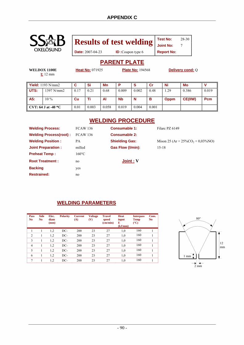
APPENDIX C

Test No: 28-30 Results of test welding Joint No: 7

Date: 2007-04-23 ID :Coupon type 6 Report No:

PARENT PLATE WELDOX 1100E Heat No: 071925 Plate No: 194568 Delivery cond: Q t: 12 mm Yield: 1193 N/mm2 C Si Mn P S Cr Ni Mo V UTS: 1397 N/mm2 0.17 0.21 0.68 0.009 0.002 0.48 1.29 0.386 0.019

A5: 10 % Cu Ti Al Nb N B Oppm CE(IIW) Pcm

CVT: 64 J at -40 *C 0.01 0.003 0.058 0.019 0.004 0.001

WELDING PROCEDURE

Welding Process: FCAW 136 Consumable 1: Filarc PZ 6149

Welding Process(root) : FCAW 136 Consumable 2:

Welding Position : PA Shielding Gas: Mison 25 (Ar + 25%CO2 + 0,03%NO)

Joint Preparation : milled Gas Flow (l/min): 15-18

Preheat Temp : 160°C

Root Treatment : no Joint : V

Backing yes

Restrained: no

WELDING PARAMETERS Pass

No Side No

Elec. diam (mm)

Polarity Current (A)

Voltage (V)

Travel speed (cm/min)

Heat input E (kJ/mm)

Interpass Temp (°C)

Cons. No

1 1 1,2 DC- 200 23 27 1,0 160 1 2 1 1,2 DC- 200 23 27 1,0 160 1 3 1 1,2 DC- 200 23 27 1,0 160 1 4 1 1,2 DC- 200 23 27 1,0 160 1 5 1 1,2 DC- 200 23 27 1,0 160 1 6 1 1,2 DC- 200 23 27 1,0 160 1 7 1 1,2 DC- 200 23 27 1,0 160 1

12 mm

80°

1 mm

2 mm

- 90 -

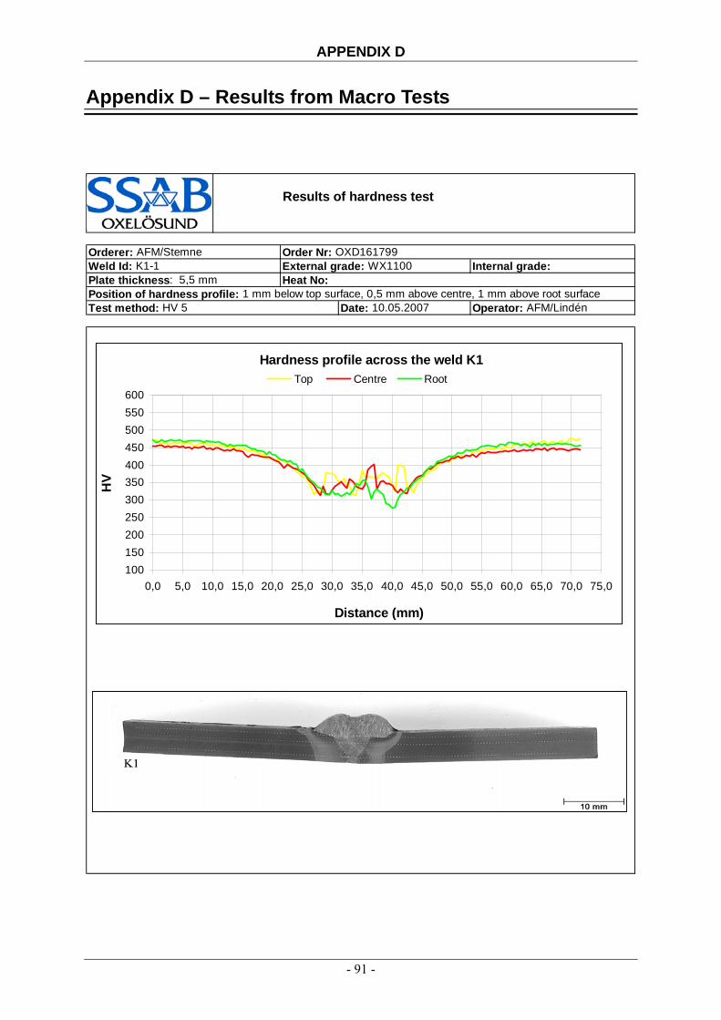
APPENDIX D

Appendix D – Results from Macro Tests

Results of hardness test

Orderer: AFM/Stemne Order Nr: OXD161799Weld Id: K1-1 External grade: WX1100 Internal grade: Plate thickness: 5,5 mm Heat No: Position of hardness profile: 1 mm below top surface, 0,5 mm above centre, 1 mm above root surfaceTest method: HV 5 Date: 10.05.2007 Operator: AFM/Lindén

Hardness profile across the weld K1

100150200250300350400450500550600

0,0 5,0 10,0 15,0 20,0 25,0 30,0 35,0 40,0 45,0 50,0 55,0 60,0 65,0 70,0 75,0

Distance (mm)

HV

Top Centre Root

- 91 -

APPENDIX D

Results of hardness test

Orderer: AFM/Stemne Order Nr: OXD161799Weld Id: K1-2 External grade: WX1100 Internal grade: Plate thickness: 5,5 mm Heat No: Position of hardness profile: 1 mm below top surface, 0,5 mm above centre, 1 mm above root surfaceTest method: HV 5 Date: 23.05.2007 Operator: AFM/Lindén

Hardness profile across the weld K1-2

100150200250300350400450500550600

0,0 5,0 10,0 15,0 20,0 25,0 30,0 35,0 40,0 45,0 50,0 55,0 60,0 65,0 70,0 75,0

Distance (mm)

HV

Top Centre Root

- 92 -

APPENDIX D

Results of hardness test

Orderer: AFM/Stemne Order Nr: OXD161799Weld Id: K2 External grade: WX960 Internal grade: Plate thickness: 6 mm Heat No: Position of hardness profile: 1 mm below top surface, 0,5 mm above centre, 1 mm above root surfaceTest method: HV 5 Date: 10.05.2007 Operator: AFM/Lindén

Hardness profile across the weld K2

100150200250300350400450500550600

0,0 5,0 10,0 15,0 20,0 25,0 30,0 35,0 40,0 45,0 50,0 55,0 60,0 65,0 70,0 75,0

Distance (mm)

HV

Top Centre Root

- 93 -

APPENDIX D

Results of hardness test

Orderer: AFM/Stemne Order Nr: OXD161799Weld Id: K3 External grade: WX1100 Internal grade: Plate thickness: 5,5 mm Heat No: Position of hardness profile: 1 mm below top surface, 0,5 mm above centre, 1 mm above root surfaceTest method: HV 5 Date: 10.05.2007 Operator: AFM/Lindén

Hardness profile across the weld K3

100150200250300350400450500550600

0,0 5,0 10,0 15,0 20,0 25,0 30,0 35,0 40,0 45,0 50,0 55,0 60,0 65,0 70,0 75,0

Distance (mm)

HV

Top Centre Root

- 94 -

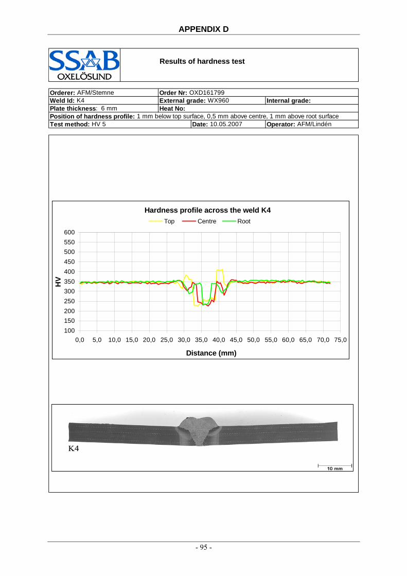
APPENDIX D

Results of hardness test

Orderer: AFM/Stemne Order Nr: OXD161799Weld Id: K4 External grade: WX960 Internal grade: Plate thickness: 6 mm Heat No: Position of hardness profile: 1 mm below top surface, 0,5 mm above centre, 1 mm above root surfaceTest method: HV 5 Date: 10.05.2007 Operator: AFM/Lindén

Hardness profile across the weld K4

100150200250300350400450500550600

0,0 5,0 10,0 15,0 20,0 25,0 30,0 35,0 40,0 45,0 50,0 55,0 60,0 65,0 70,0 75,0

Distance (mm)

HV

Top Centre Root

- 95 -

APPENDIX D

Results of hardness test

Orderer: AFM/Stemne Order Nr: OXD161799Weld Id: K5 External grade: WX1100 Internal grade: Plate thickness: 12 mm Heat No: Position of hardness profile: 1 mm below top surface, 0,5 mm above centre, 1 mm above root surfaceTest method: HV 5 Date: 10.05.2007 Operator: AFM/Lindén

Hardness profile across the weld K5

100150200250300350400450500550600

0,0 5,0 10,0 15,0 20,0 25,0 30,0 35,0 40,0 45,0 50,0 55,0 60,0 65,0 70,0 75,0

Distance (mm)

HV

Top Centre Root

- 96 -

APPENDIX D

Results of hardness test

Orderer: AFM/Stemne Order Nr: OXD161799Weld Id: K6 External grade: WX1100 Internal grade: Plate thickness: 12 mm Heat No: Position of hardness profile: 1 mm below top surface, 0,5 mm above centre, 1 mm above root surfaceTest method: HV 5 Date: 10.05.2007 Operator: AFM/Lindén

Hardness profile across the weld K6

100150200250300350400450500550600

0,0 5,0 10,0 15,0 20,0 25,0 30,0 35,0 40,0 45,0 50,0 55,0 60,0 65,0 70,0 75,0

Distance (mm)

HV

Top Centre Root

- 97 -

APPENDIX E

Appendix E - Specimen Photos

- 98 -

APPENDIX E

- 99 -