Optimization of Low-Thrust Gravity-Assist Trajectories with a Reduced Parameterization of the Thrust Vector

Chit Hong Yam James M. Longuski

School of Aeronautics and Astronautics

Purdue University West Lafayette, Indiana 47907

Paper AAS 05-375

2005 AAS/AIAA Astrodynamics Specialists Conference

Lake Tahoe, CA, August 7-11, 2005

AAS Publications Office, P.O. Box 28130, San Diego, CA 92198

AAS 05-375

1

OPTIMIZATION OF LOW-THRUST GRAVITY-ASSIST TRAJECTORIES WITH A REDUCED PARAMETERIZATION OF

THE THRUST VECTOR*

Chit Hong Yam† and James M. Longuski‡

A low-thrust trajectory can be modeled as a sequence of impulses (ΔV) connected by conic arcs. Each ΔV is described by at least three coordinates. We investigate new ways of parameterizing the ΔV coordinates when optimizing low-thrust gravity-assist trajectories. For the ΔV magnitude coordinate, we use a set of on/off times to control the thrusting and coasting period of the trajectory. For the ΔV angles, we use parametric functions of time (i.e. Chebyshev Series) to approximate the optimal thrust angles. With the appropriate choice of parameters, the number of optimization variables and constraints (and thus convergence speed) may be reduced significantly, with albeit a small sacrifice in accuracy. The new formulation is particularly useful in mission design trade studies where hundreds of trajectories may be optimized over a wide range of design parameters (e.g. launch window).

INTRODUCTION

In 1998, NASA launched the first spacecraft which employs ion propulsion as the primary propulsion system: Deep Space 1. With a specific impulse (Isp) of about ten times more than a chemical rocket,1 the Deep Space 1’s NSTAR thruster provides a large saving in propellant mass (and thus mission costs). Following on the Deep Space 1 mission, two missions are expected to further demonstrate the effectiveness of ion propulsion: SMART-1 has been launched to and is orbiting around the Moon, while the DAWN mission is planned to be launched to Ceres and Vesta in 2006.

Low-thrust missions have been proposed in the literature for over forty years.2-23 In 1999, Sims and Flanagan24 proposed modeling low-thrust trajectories as a sequence of impulsive maneuvers (ΔV) connected by conic arcs. Using such a model, several papers have been written on design and optimization of low-thrust, gravity-assist (LTGA) trajectories to various destinations in the Solar System.13,17,20-24

The size of the problem in optimizing LTGA trajectories (with the Sims and Flanagan model) can range from about 100 optimization variables and 50 constraints (for a typical single-leg mission, such as an Earth-Mars mission), to nearly 2000 optimization variables and over 800 constraints (for a 45-year Earth-Mars cycler20). As the number of variables and constraints increase, the time required for finding an optimal solution also increases. * Copyright © 2005 by Chit Hong Yam and James M. Longuski. Published by the American Astronautical Society with permission. † Doctoral Candidate, School of Aeronautics and Astronautics, Purdue University, West Lafayette, Indiana 47907-2023. Student

Member AIAA. Email: cyam@purdue.edu ‡ Professor, School of Aeronautics and Astronautics, Purdue University, West Lafayette, Indiana 47907-2023. Associate Fellow

AIAA; Member AAS. Email: longuski@ecn.purdue.edu

2

Thus it would be beneficial if we could formulate the problem with fewer variables and constraints, even with a (reasonably) less accurate answer.

Based on the Sims and Flanagan model, McConaghy and Longuski25 have investigated four coordinates systems for the ΔV vectors (namely Cartesian, Spherical, Magnitude and Cartesian, and Magnitude and Direction-Vector Coordinates). In their examples, Spherical Coordinates are used to get fast and accurate results when a good initial guess is available; when the initial guess is bad, Cartesian Coordinates are used to first find a feasible solution, followed by Spherical Coordinates to find an optimal solution.

The approach proposed by McConaghy and Longuski25 works well when we are optimizing a single trajectory. This approach alone, however, may not fit the needs of mission designers looking at a wide range of design space (e.g. launch dates, time-of-flight, and hardware parameters) with dozens or hundreds of optimized trajectories. In a parametric study, speed is often more important than accuracy. The mission designers would rather see the trends of the mission quickly (accepting a few kilograms of error) than to wait for hours for accurate results. If we are interested in a particular trajectory, we can perform a follow up study to sharpen the accuracy.

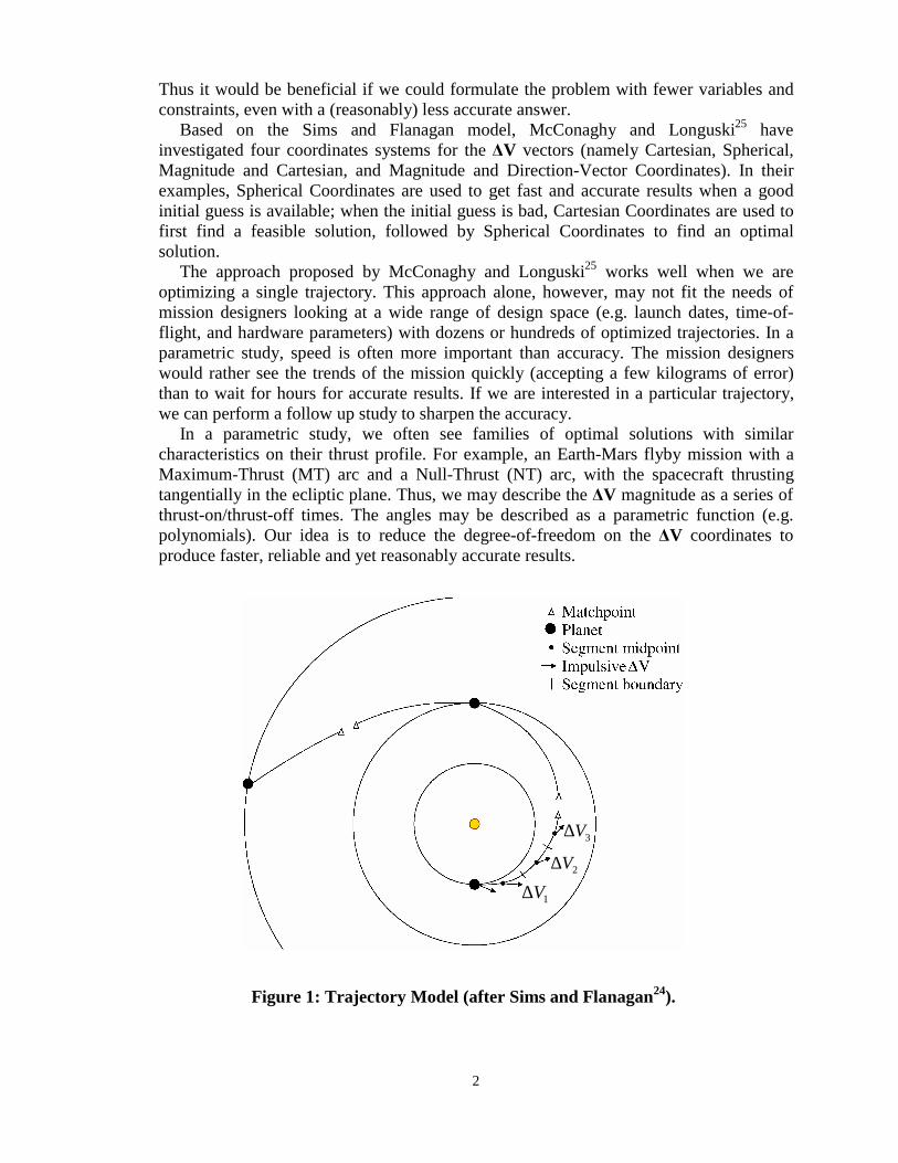
In a parametric study, we often see families of optimal solutions with similar characteristics on their thrust profile. For example, an Earth-Mars flyby mission with a Maximum-Thrust (MT) arc and a Null-Thrust (NT) arc, with the spacecraft thrusting tangentially in the ecliptic plane. Thus, we may describe the ΔV magnitude as a series of thrust-on/thrust-off times. The angles may be described as a parametric function (e.g. polynomials). Our idea is to reduce the degree-of-freedom on the ΔV coordinates to produce faster, reliable and yet reasonably accurate results.

1V∆2V∆

3V∆

1V∆2V∆

3V∆

Figure 1: Trajectory Model (after Sims and Flanagan24).

3

TRAJECTORY MODEL AND THE OPTIMIZATION PROBLEM

The Sims and Flanagan model24 divides each planet-planet leg of the low-thrust trajectory into segments of equal duration. (For a direct mission without gravity assist, there is only one leg.) The thrusting on each segment is modeled by an impulsive ΔV at the midpoint of the segment, with conic arcs between the impulses. Each leg is propagated half-way forward from the initial body and half-way backward from the final body. In order to have a feasible trajectory, the forward- and backward-propagated half-legs must meet at a match-point time in the middle of the leg. Figure 1 illustrates the key characteristics of the Sims and Flanagan trajectory model.

We call our trajectory optimization software (which is based on the Sims and Flanagan model) the Gravity-Assist Low-thrust Local Optimization Program (GALLOP). The optimization variables in GALLOP include the following:

1) The Julian dates at the launch, flyby, and arrival bodies, 2) The launch V∞ (or the outgoing inertial velocity vector at launch), 3) The arrival V∞ (or the incoming inertial velocity vectors at all of the postlaunch

bodies), 4) The spacecraft mass at each body, 5) The flyby altitude at the gravity-assist bodies, 6) The B-plane angle at the gravity-assist bodies, 7) The Julian dates and positions of the nodes, velocities and masses of the spacecraft

when it crosses the nodes (when there are nodes in the trajectory), and 8) The ΔV parameters on each leg. In this paper, we introduce (or modify) two new sets of optimization variables, 7) and

8), which are not available in the literature.13,17,20-26 We will discuss the meaning of the “node” and the “ΔV parameters” in the section titled “Parameterization of the Thrust Vector”.

The optimization program can alter these variables to find feasible and optimal solutions of the given problem. A feasible solution means the variables satisfy the constraints. These constraints include:

1) The magnitude of the ΔV on a segment cannot exceed a maximum which depends

on the thrust, mass-flow rate, the segment duration, the engine duty cycle and the spacecraft mass,

2) The flyby altitude must be above a minimum height (if there is any planetary flyby in the trajectory), and

3) The position (x, y, z), velocity (Vx, Vy, Vz), and the spacecraft mass of the forward- and backward-propagated legs must be equal at a prespecified matchpoint (usually in the middle of the leg). (i.e. the seven state-mismatches between the forward- and backward- propagated legs at the matchpoint are equal to zero.)

Within the feasible set of solutions, the optimizer can find a solution which maximizes

the final mass of the spacecraft (the objective function).

4

OPTIMIZATION SOFTWARE

Our trajectory optimization program (GALLOP) uses the numerical nonlinear programming optimization software NPOPT.27,28 NPOPT implements the sequential quadratic programming (SQP) method to find a locally optimal solution to an optimization problem. In our experience, the speed and robustness of convergence to an optimal solution relies on the analytic derivatives of the objective and constraint functions. If instead, we are using finite differences to approximate the derivative, the optimization process will be much slower and less robust (i.e. it may fail to converge in some cases). In addition, the smoothness of the objective and of the constraint functions may also affect the behavior of NPOPT.28 (Thus, any changes in the parameterization of the thrust vector necessarily require the analytic derivatives for the new variables.)

Figure 2 shows a simplified schematic of GALLOP. Note that Fig. 2 does not include every process of GALLOP (such that the scaling of the optimization variables). Starting from the User’s Input, GALLOP reads in trajectory and spacecraft information (e.g.

Figure 2: Schematic of GALLOP.

Initial Guess and bounds of the Opt. Var.

NPOPT

Inputs from the User

• Engine parameters, launch, encounter and arrival bodies, number of segments on each leg

• Initial Guess, Upper and Lower Bounds of the Optimization Variables

• Choice of Reference Frame on each leg – Inertial, VCN, RTH

• Choice of Coordinate Systems – Cartesian, Spherical, MCC, MDV

• Choice of Functional Form – N-Vector, On/Off, Chebyshev

GALLOP

Objective Function

Maximize the Final Mass

Constraint Function For each leg, propagate the trajectory forward and backward, calculate the state-mismatch at the matchpoint (usually in the middle of a leg). See Fig. 3 for details.

Final Mass, Gradient

State-Mismatches, Jacobian

Optimal Solution Found? If not, reiterate with a new set of Opt. Var.

5

engine parameters, launch and arrival bodies), optimization variables (mentioned in the previous section) and their upper and lower bounds, the ΔV reference frame, the ΔV coordinate system, and the ΔV functional form. GALLOP evaluates the objective-function and constraint-function values. These values include the final mass (and its derivatives with respect to the optimization variables) and the state-mismatches on each leg (and their derivatives with respect to the optimization variables), pass to NPOPT together with the initial guess and the bounds of the optimization variables. (For simplicity of the illustration, we do not include constraints on the maximum ΔV magnitudes and constraints on the flyby altitudes.)

NPOPT evaluates this set of variables to determine its feasibility and optimality (from

the objective-function and constraint-function values). If this set of variables satisfies the feasibility tolerance and optimality tolerance (unless otherwise specified, both are set to 10-6), NPOPT returns with an EXIT condition “Optimal Solution Found.” Otherwise, NPOPT returns with a new set of variables (found by the derivatives of the objective and

Figure 3: Converting the ΔV Parameters to the Inertial X, Y, Z components of ΔV inside the Constraint Function of GALLOP.

Evaluate the ΔV Function Extract the ΔV Coordinate-Values from the given ΔV parameters.

• No change if the user has specified the ΔV-functional-form as N-Vector.

• If ΔV-functional-form is On/Off, (Ton, Toff) → (ΔV1,…,ΔVN)

• If ΔV-functional-form is Chebyshev, (c0, c1,…) → (θ1,…, θN)

Coordinate System Conversion

• No change if the user has specified the ΔV in Cartesian Coordinates.

• If the ΔV is specified in Spherical Coordinates (same for MCC and MDV), then convert it to Cartesian Coordinates.

(ΔV, θ, ψ) → (ΔVx, ΔVy, ΔVz)

Reference Frame Transformation

• No change if the user has specified the ΔV in the Inertial Frame.

• If the ΔV is specified in Velocity-Cornormal-Normal Frame (same for R-Theta-H Frame), then transform it to the Inertial Frame.

(ΔVvcn) → (ΔVxyz)

Inertial X, Y, Z components of the ΔV: (ΔVx, ΔVy, ΔVz)

Propagate forward and backward, calculate the state-mismatch

ΔV Parameters given as Optimization Variables

6

constraint functions) to GALLOP and reiterates, until it finds an optimal solution or it reaches a major iteration limit (or various other EXIT condtions28).

Inside the constraint function of GALLOP, the spacecraft trajectory is propagated forward and backward to their matchpoints on each leg. To do so, one must convert the ΔV parameters (given as optimization variables) to the X, Y, Z components of the ΔV vectors in the inertial reference frame (Ecliptic and Equinox of J2000). At the midpoint of each segment, the inertial spacecraft velocities after the maneuver can be found by simply adding the inertial spacecraft velocities before the maneuver to the inertial ΔVx, ΔVy and ΔVz (The inertial position of the spacecraft before and after the maneuver does not change). With the new spacecraft states (inertial position and velocities after the maneuver), the trajectory is propagated as a conic arc to the next segment midpoint to perform the next ΔV, until it reaches the prespecified matchpoint (usually in the middle of the leg).

Figure 3 illustrates the key steps in converting the ΔV parameters to the inertial ΔVx, ΔVy and ΔVz on each segment. The ΔV parameters are first converted to the ΔV coordinate-values on each segment (e.g. converting the thrust-on and thrust-off times Ton and Toff to the ΔV magnitudes on each segment: ΔV1, ΔV2,…, ΔVN), by evaluating the ΔV functions corresponding to each ΔV coordinates. We will discuss the meaning of the “ΔV parameters” and “ΔV coordinates” in the section titled “Parameterization of the Thrust Vector”. Next, the ΔV are transformed to Cartesian Coordinates (when the ΔV parameters are not specified in Cartesian Coordinates). Finally, any ΔV written in a non-inertial frame are transformed to the X, Y, Z components in the inertial frame: ΔVx, ΔVy and ΔVz.

DELTA-V REFERENCE FRAME

In some of the solutions (e.g. Earth-Jupiter Rendezvous Mission) we have found, the thrust is along the velocity vector, followed by a coast until rendezvous with the planet. In such cases, specifying the ΔV vector in a spacecraft rotating frame (instead of in the inertial frame) may be beneficial in the optimization process. Figure 4 defines the vectors V, C, N and the vectors r, θ, h in a spacecraft orbital plane. We added two spacecraft rotating frames to GALLOP: Velocity-Conormal-Normal (as defined by the vectors: V, C, N) and R-Theta-H (as defined by the vectors: r, θ, h).

User can easily specify an “in-plane, tangential steering law” by letting the clock angle θ to zero and the cone angle ψ to 90 degrees in the VCN frame. If, for example, the ΔV vectors are written in the inertial frame, a tangential steering law cannot be as easily described as in the case of the ΔV vectors written in the VCN frame.

PARAMETERIZATION OF THE THRUST VECTOR

An impulsive ΔV vector on a particular segment can be specified as three (or four) scalars of ΔV coordinates. By the “ΔV coordinates”, we mean the X, Y, Z components of the ΔV vector (ΔVx, ΔVy, ΔVz) if we are using Cartesian Coordinates; If we are using Spherical Coordinates, we mean the ΔV magnitude, clock and cone angles of the ΔV vector (ΔV, θ, ψ). [Reference 25 also discusses Magnitude and Cartesian Coordinates

7

(MCC) and Magnitude and Direction-Vector Coordinates (MDV). We will not study these two coordinate systems in this paper.] Note that these ΔV coordinates can be written in a reference frame other than the inertial frame, such as the VCN frame.

For each leg, each of the three ΔV coordinates, (ΔVx, ΔVy, ΔVz) or (ΔV, θ, ψ), can be

written as a function of the segment number, or the fractional leg-duration x ranging from 0 to 1. For example, consider the ΔV magnitude coordinate for an Earth-Jupiter Rendezvous mission in Figure 5. There are sixty ΔV values (denoted as {ΔVi}i=1,…,60), one for each segment. These sixty ΔV values, {ΔVi}, can be written as {ΔVi} = ΔV(i) or ΔV( x ). The ΔV values on each segment are evaluated from a ΔV-function, ΔV(i). Similarly, the θ and ψ values on each segments are evaluated from a θ-function, θ(i), and a ψ-function, ψ(i), respectively. The functions on the ΔV coordinates can be piecewise polynomials, trigonometric functions, etc.

TABLE 1 OPTIMIZATION VARIABLES ASSOCIATED WITH THE ΔV VECTORS FOR

FIVE DIFFERENT FORMULATIONS Optimization Variables N-Vector On/Off Node Chebyshev Node +

Chebyshev ΔVx, ΔVy, ΔVz

üa ΔV Magnitude

üb ü

Clock and Cone Angles (θ, ψ)

üb ü ü Toggle-Times (Ton and Toff)

ü Time and the 7-Statec of the Node at Switch-On/Off Times

ü

ü

Coefficients on the Chebyshev Series (c0, c1,…,ck)

ü ü a If we are using Cartesian Coordinates. b If we are using Spherical Coordinates. c Includes the position of the node, and the velocity and mass of the spacecraft.

Figure 4: Definition of the VCN (Velocity, Conormal, Normal) and

RTH (r, θ, h) Frames.

r (radial)

V (Velocity)

(Local Horizontal Plane)

N = h (Angular Momentum)

(h = r x V)

C = N x V

θ

(Attracting Center)

8

Besides the independent variable i (or x ), the ΔV functions also depend on a set of “ΔV parameters” (treated as optimization variables). A simple example of the ΔV parameters is the ΔV coordinates themselves, i.e. (ΔVx, ΔVy, ΔVz) or (ΔV, θ, ψ) are optimization variables, meaning that ΔV(i) = ΔVi, θ(i) = θi and ψ(i) = ψi (called the “N-vector” function). Another example of the ΔV parameters is the coefficients c0 and c1 of a linear function. The ΔV coordinates on each segment are then calculated by the formula c0 + c1 x . Table 1 summarizes the optimization variables (or ΔV parameters) of five formulations studied in this paper.

In previous work and in the current paper, several formulations are used to parameterize the ΔV vectors. In this section, we define these formulations before showing their relative effectiveness in the numerical section.

N-Vector Formulation (Function)

By the N-Vector Formulation (or the N-Vector function), we mean the ΔV coordinates on each segment (ΔV, θ, ψ) or (ΔVx, ΔVy, ΔVz) are optimization variables (or ΔV parameters). The relationship between the ΔV coordinates and the ΔV parameters are simply:

( ) ( ) ( )i i iV i V i iθ θ ψ ψ∆ = ∆ = = (1)

if we are using Spherical Coordinates (similarly for Cartesian Coordinates). The optimizer can vary the ΔV coordinates, subject to the maximum-allowable-ΔV

constraint (determined by the spacecraft mass and the engine parameters). For a

0 5 10 15 20 25 30 35 40 45 50 55 600

0.1

0.2

0.3

0.4

0.5

0.6

0.7

segment

∆ V m

agni

tude

(km

/s)

MaximumInitial guessSolution

Figure 5: ΔV Magnitude Coordinate of an Earth-Jupiter Rendezvous

Mission.

9

trajectory with a total of N segments, there are 3N variables and N nonlinear constraints associated with the ΔV coordinates in the N-Vector Formulation. The N-Vector Formulation was the “Original Formulation” used in the literature to design LTGA trajectories (following the Sims and Flanagan model).13,17,20-26

On/Off Formulation (Function)

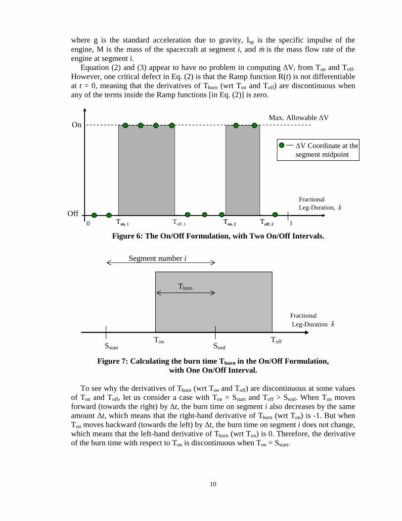
The “On/Off Formulation” uses a set of thrust-on/off times to control the thrusting and coasting period of the trajectory. The ΔV magnitude coordinate on each leg is parameterized by specifying a set of “toggle-times”: {Ton,1 Toff,1 Ton,2 Toff,2 ……,Ton,k Toff,k}, where k is the number of thrust-intervals. These toggle-times are treated as optimization variables (instead of the ΔV magnitudes). From our experience, optimal trajectories often have thrusting at the maximum level or coasting, with only short periods of intermediate thrust (for example the ΔV profile in Fig. 5). Thus, the On/Off Formulation assumes the ΔV magnitude is at maximum when a thrust-interval covers the whole segment. Figure 6 gives an example of the ΔV magnitude coordinate with two on/off pulses.

For a trajectory with a total of k thrust-intervals and N segments (usually k<<N), the number of variables associated with the ΔV reduces from 3N to 2N+2k. Since the ΔV are always smaller than or equal to the maximum allowable ΔV, there are no nonlinear constraints associated with the ΔV magnitude coordinate (which removes N nonlinear constraints). Since the On/Off Formulation parameterizes the ΔV magnitude coordinate, it can only be used with Spherical Coordinates (but not Cartesian Coordinates).

To find the relationship between the ΔV magnitude coordinates and the ΔV parameters (Ton,k and Toff,k), consider an example in Figure 7. For simplicity of the illustration, assume that there is only one on/off interval, ranging from Ton to Toff. The burn time on segment i, is the region covered by the on/off interval between Sstart and Send (the start time and the end time of segment i, in fractional leg-duration). In the case of Fig. 7, the burn time is equal to Send − Ton. In general, the burn time Tburn on segment i is equal to:

( ) ( ) ( )burn off on start on off endT R R T T R S T R T S = − − − − − (2)

where R(t) = max(0, t) is the Ramp function, Sstart = (i −1)/N and Send = i/N for a leg with N segments.

We note that Eq. (2) can also be written as a form with several logical expressions (e.g. if Toff > Send). But since we also have to compute the derivatives of the burn time with respect to the ΔV parameters (Ton and Toff), it is more convenient to write Eq. (2) into a single formula with the Ramp function.

From the burn time Tburn, the ΔV on segment i is therefore given by the rocket equation:

lni spburn

MV gIM mT

∆ = −

(3)

10

where g is the standard acceleration due to gravity, Isp is the specific impulse of the engine, M is the mass of the spacecraft at segment i, and m is the mass flow rate of the engine at segment i.

Equation (2) and (3) appear to have no problem in computing ΔVi from Ton and Toff. However, one critical defect in Eq. (2) is that the Ramp function R(t) is not differentiable at t = 0, meaning that the derivatives of Tburn (wrt Ton and Toff) are discontinuous when any of the terms inside the Ramp functions [in Eq. (2)] is zero.

To see why the derivatives of Tburn (wrt Ton and Toff) are discontinuous at some values of Ton and Toff, let us consider a case with Ton = Sstart and Toff > Send. When Ton moves forward (towards the right) by Δt, the burn time on segment i also decreases by the same amount Δt, which means that the right-hand derivative of Tburn (wrt Ton) is -1. But when Ton moves backward (towards the left) by Δt, the burn time on segment i does not change, which means that the left-hand derivative of Tburn (wrt Ton) is 0. Therefore, the derivative of the burn time with respect to Ton is discontinuous when Ton = Sstart.

Figure 7: Calculating the burn time Tburn in the On/Off Formulation, with One On/Off Interval.

Sstart Send Ton Toff

Segment number i

Fractional Leg-Duration x

Tburn

ΔV Coordinate at the segment midpoint

Fractional Leg-Duration, x

T on, 1 T off , 1 T on, 2 T off , 2 1 T on, 1 T on, 2 T off , 2

Max. Allowable ΔV

Figure 6: The On/Off Formulation, with Two On/Off Intervals.

On

Off 0

11

Optimization software generally does not behave well when there are discontinuous derivatives near the solution space. Following the approach described in Ref. 26 (when introducing the multiple-engine model), we attempt to improve the convergence behavior by replacing the Ramp function R(t) in Eq. (2) with the smooth Ramp function Rs(t):

0 for

( ) for ( ) otherwise

s

t aR t t t a

p t

≤ −= ≥ +

(4)

where a is a smoothing parameter, p(t) is an unique 6th degree polynomial which connects Rs(t) = 0 and Rs(t) = t smoothly such that Rs(t) is differentiable at every point.

Changing the smoothing parameter a affects the “sharpness” of Rs(t), which means that the more discontinuous as it is seen by the optimizer. The larger the parameter a, the smoother the derivatives of the burn time are. However, with a larger a value, the calculation of the burn time in Eq. (2) might get less accurate (with some residue value). Therefore, guideline from practical experience is needed for choosing a suitable a value in solving a particular problem.

Even with many foreseeable challenges, we have programmed the On/Off Formulation in GALLOP. In our experience, the behavior of convergence for the On/Off Formulation is not predictable: sometimes it converges faster (with accurate results) than the N-Vector Formulation, but often we see that the On/Off Formulation fails to converge (or converges to a sub-optimal point), especially in cases where the dates on the planetary encounter are free (i.e. with no upper and lower bounds). Even after we introduce the smoothing parameter a (with a ranges from 10-8 to 0.1 in segment-duration), the convergence behavior is still quite unpredictable. With the poor performance, we shall, therefore, not show any numerical results of the On/Off Formulation.

Node Formulation

With the lessons learned from the On/Off Formulation, we find that putting thrust on/ off points inside a leg might not be a good idea. Instead, we break a single-leg (for example) trajectory into a multiple-leg trajectory, with the thrust-on and thrust-off points separating the legs.

For example, let us consider an Earth-Jupiter Rendezvous mission in Fig. 8. The first leg of the trajectory launches from the Earth goes around the Sun for about one and a half revolution, with the spacecraft thrusting at its maximum thrust level, until it reaches the “Thrust Off” point in the figure. The second leg consists of two segments of coasting, until it reaches the “Thrust On” point. Finally, the spacecraft turns on the engine again from the “Thrust On” point to rendezvous with the arrival planet, Jupiter.

We call the “Thrust Off” point (and “Thrust On” point) a “Node”. A Node is a control point which acts like a body (or planet), except that a Node does not have a prescribed orbit around the Sun. Since GALLOP propagates the spacecraft trajectory forward from the launch body and backward from the encounter (or arrival) body, the spacecraft will always be able to fly through a Node (although it might not fly through the matchpoints).

12

Each Node has eight scalars associated with it: the encounter time (Julian Date) at the

Node, the inertial position vector (X, Y, Z) of the Node, the spacecraft inertial velocity vector (Vx, Vy, Vz) when it passes through the Node and the spacecraft mass when it passes through the Node. These eight optimization variables may have upper and lower bounds (for setting reasonable ranges), but for the purpose of modeling the Thrust On and Thrust Off times, we let these eight variables free (the constraints on the state-mismatch ensure a feasible trajectory).

In order to set all the ΔV magnitudes on a leg to maximum, we use two Toggle-Times: with Ton = 0 (start of a leg) and Toff = 1 (end of a leg). The values on Ton and Toff are kept frozen to 0 and 1 respectively, meaning that the optimization software will not change Ton and Toff during the optimization run.

Although the Node Formulation does not really parameterize the ΔV magnitude, it can replace the On/Off Formulation. One advantage of using the Node Formulation (instead of On/Off) is that the derivatives of the constraints (state-mismatches) with respect to the eight new variables (associated with the Node) are continuous. For a trajectory with N segments, the Node Formulation replaces the N ΔV magnitudes with 8k variables associated with the Node, where k is the number of Nodes added to the trajectory.

Thrust Angles Parameterizations: Chebyshev Formulation

The coordinates of the ΔV angles (clock angle θ and cone angle ψ) can be modeled as parametric functions of time (or functions of the fractional leg-duration x ). Figure 9 shows a sketch of a thrust angle coordinate modeled by a parametric function.

In particular, we use the Chebyshev Series (a linear combination of the Chebyshev polynomials) to model the ΔV angles coordinates. (For an excellent introduction to

-5 -4 -3 -2 -1 0 1 2 3 4

-2

-1

0

1

2

3

4

5

x, AU

y, A

U

Thrust Off

Thrust On

Earth

Jupiter

Figure 8: An Earth-Jupiter Rendezvous Trajectory; Optimized using the Node Formulation.

13

Chebyshev polynomials, see Mason and Handscomb.29) A Chebyshev Series of degree k is defined as:

0 0 1 1( ) ( ) ... ( )k kc T u c T u c T u+ + + (5)

where Tk(u) is the Chebyshev polynomial of degree k, and u = 2 x -1 is the independent variable of the Chebyshev polynomial, ranging from -1 to 1.

Each Chebyshev Series is specified by k+1 parameters: {c0,c1,…,ck}. These k+1 parameters (or coefficients) are optimization variables (instead of the thrust angles on each segment) in the Chebyshev Formulation (the ΔV magnitudes on each segment are optimization variables). If the clock and cone angles coordinates (θ and ψ) both use the Chebyshev Formulation (of degree kθ and kψ respectively), then for a trajectory of N segments, the number of variables associated with the ΔV vectors reduces from 3N to N+kθ+kψ+2 (usually kθ and kψ <<N).

Node + Chebyshev Formulation

In the Node + Chebyshev Formulation, both the ΔV magnitude and the angles are parameterized. The ΔV magnitude is parameterized by the thrust-on and thrust-off Nodes; the thrust angles are parameterized by the Chebyshev Series. The Node + Chebyshev Formulation reduces the number of variables significantly compared to the N-Vector Formulation. The Nodes break the trajectory into thrusting and coasting legs, so that the Chebyshev Series solely models the thrusting angles, preventing the angles from drifting off track during the coasting segments.

NUMERICAL RESULTS

To demonstrate the effectiveness of the new formulations, we present some test cases in this section.

Figure 9: Modeling a Thrust Angle Coordinate with a Parametric Function.

Clock Angle, θ

Fractional Leg-Duration, x

θ( x ,c0,c1,…,cn)

θ Coordinate at the segment midpoint

14

Node Formulation Test Case: Earth-Jupiter Flyby Mission

We begin our numerical experiments with testing the speed and accuracy of the Node Formulation. The problem we are trying to optimize is an Earth-Jupiter Flyby Mission. Table 2 summarizes the engine parameters of this mission. We assume that the spacecraft is propelled by ion engines (as described in Table 2) powered by nuclear energy, meaning that the power available to the thrusters is a constant (unlike the case of solar electric propulsion).

Petropoulos et al.30,31 developed a Shape-Based approach to allow automated rapid search of low-thrust gravity-assist trajectories. The Shape-Based approach is implemented in a program called STOUR-LTGA. We often use trajectories found by STOUR-LTGA as the initial guesses to find the first optimal solutions in GALLOP. Table 3 summarizes the characteristics of an Earth-Jupiter flyby trajectory. Using the initial guess found by STOUR-LTGA, GALLOP finds an optimal solution by the N-Vector Formulation and the Node Formulation. Note that the Earth launch date, the Jupiter arrival date, the launch V∞ and the initial mass are kept frozen during the optimization.

Figure 10 shows the ΔV magnitude coordinate of the Earth-Jupiter flyby mission. We notice that the ΔV magnitude coordinate can be divided into two phases: Maximum thrust and Coast. Therefore in the Node Formulation, a Node is placed in between of the thrusting and coasting phase of the trajectory, breaking the trajectory into two legs. We assume that the first leg of the trajectory is at maximum thrust and the second leg is coast. Thus, we replace the 60 ΔV magnitude coordinates with a Node (which has eight variables associated with it). In addition to the ΔV magnitude, since the second leg is purely coasting, we can reduce the number of segments (on the coasting leg) from 23 down to 2.

TABLE 2: NUCLEAR ELECTRIC SPACECRAFT

PARAMETERS Parameter Values Power Available to the Thrusters 95 kW Specific Impulse 6,000 s Overall Efficiency 70 % Thrust 2.26 N Mass Flow Rate 38.4 mg/s

TABLE 3: EARTH-JUPITER FLYBY MISSION PARAMETERS

Characteristics Initial Guessa Optimal Solution Earth Launch Dateb April 21, 2022 April 21, 2022 Launch V∞

b 0.4 km/s 0.4 km/s Initial Massb 20,000 kg 20,000 kg Jupiter Arrival Dateb Dec 11, 2028 Dec 11, 2028 Jupiter Arrival V∞ 3.43 km/s 4.31 km/s Arrival Mass 13,060 kg 15,098 kg a The initial guess came from STOUR-LTGA. b Frozen during optimization.

15

Table 4 shows a comparison between the N-Vector Formulation and the Node

Formulation. By making some simplifying assumptions on the ΔV magnitude, we reduce the number of variables from 190 on the N-Vector Formulation to 100 on the Node Formulation. The number of nonlinear constraints also reduces to 14 (by removing the excess ΔV magnitude constraints on each segment). The optimized final mass on the Node Formulation is 0.8 kg higher than that of the N-Vector Formulation. We do not claim that the Node Formulation finds a better solution than the N-Vector Formulation; We accept an error of 0.8 kg in Node Formulation.

The run time on the N-Vector Formulation is shorter than the Node Formulation by 62 sec. One possible explanation of this counter-intuitive result is that the N-Vector Formulation keeps the degree of freedom in changing the ΔV magnitude, while the Node Formulation has a restricted form on the ΔV magnitude. The dotted line in Fig. 10 shows the initial guess of the ΔV magnitude (found by STOUR-LTGA) on the N-Vector Formulation. The ΔV magnitude on the Node Formulation, however, can only be a square wave. The restricted form on the ΔV magnitude makes the initial trajectory of the Node Formulation highly infeasible and therefore, increases the run time.

TABLE 4: COMPARING THE N-VECTOR AND NODE FORMULATION ON THE

E-J FLYBY TEST CASE Formulation Number of

Optimization Variables

Number of Nonlinear

Constraints

Optimized Final Mass,

kg

Run Time, sec

N-Vector 190 67 15098.0 13 Node 100 14 15098.8 75

0 5 10 15 20 25 30 35 40 45 50 55 600

0.1

0.2

0.3

0.4

0.5

0.6

0.7

segment

∆ V m

agni

tude

(km

/s)

MaximumInitial guessSolution

Figure 10: Optimal ΔV Magnitude of an Earth-Jupiter Flyby Mission.

16

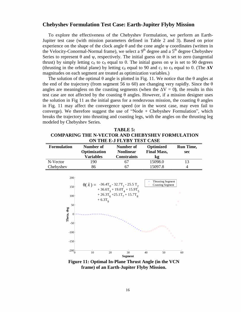
Chebyshev Formulation Test Case: Earth-Jupiter Flyby Mission

To explore the effectiveness of the Chebyshev Formulation, we perform an Earth-Jupiter test case (with mission parameters defined in Table 2 and 3). Based on prior experience on the shape of the clock angle θ and the cone angle ψ coordinates (written in the Velocity-Conormal-Normal frame), we select a 9th degree and a 5th degree Chebyshev Series to represent θ and ψ, respectively. The initial guess on θ is set to zero (tangential thrust) by simply letting c0 to c9 equal to 0. The initial guess on ψ is set to 90 degrees (thrusting in the orbital plane) by letting c0 equal to 90 and c1 to c9 equal to 0. (The ΔV magnitudes on each segment are treated as optimization variables.)

The solution of the optimal θ angle is plotted in Fig. 11. We notice that the θ angles at the end of the trajectory (from segment 56 to 60) are changing very rapidly. Since the θ angles are meaningless on the coasting segments (when the ΔV = 0), the results in this test case are not affected by the coasting θ angles. However, if a mission designer uses the solution in Fig 11 as the initial guess for a rendezvous mission, the coasting θ angles in Fig. 11 may affect the convergence speed (or in the worst case, may even fail to converge). We therefore suggest the use of “Node + Chebyshev Formulation”, which breaks the trajectory into thrusting and coasting legs, with the angles on the thrusting leg modeled by Chebyshev Series.

TABLE 5: COMPARING THE N-VECTOR AND CHEBYSHEV FORMULATION

ON THE E-J FLYBY TEST CASE Formulation Number of

Optimization Variables

Number of Nonlinear

Constraints

Optimized Final Mass,

kg

Run Time, sec

N-Vector 190 67 15098.0 13 Chebyshev 86 67 15097.8 4

0 10 20 30 40 50 60-200

-150

-100

-50

0

50

100

150

200

Segment

Thet

a, d

eg

Thrusting SegmentCoasting Segment -36.4T0 - 32.7T1 - 25.5 T2

+ 36.6T3 + 19.0T4 + 15.9T5 + 26.3T6 +25.1T7 + 15.7T8 + 6.3T9

Figure 11: Optimal In-Plane Thrust Angle (in the VCN frame) of an Earth-Jupiter Flyby Mission.

θ( x ) =

17

Earth-Jupiter Rendezvous Mission: Flight Time Trade Study

In Table 5, we note that the Chebyshev Formulation saves 9 seconds in finding an optimal solution comparing with the N-Vector Formulation (with an error of 0.2 kg). For designing a single trajectory, saving seconds of run time is not important. However, if we are interested in looking at a wide range of design space, (e.g. launch dates, and engine power) we may need to optimize dozens or even hundreds of trajectories. Saving a few seconds per run can save hours of computer process time in a large parametric study. The new parameterizations studied in this paper may be beneficial to a mission designer who is willing to sacrifice some accuracy in the solution with faster results.

We give an example of a parametric study on an Earth-Jupiter Rendezvous mission. Table 2 defines the spacecraft parameters of this mission. The encounter dates at Earth and Jupiter are free (with no bounds); while the launch V∞ is constrained to be zero. Table 6 compares the characteristics of the three formulations on this test case.

By reducing the upper bounds on the Time-of-Flight (a linear constraint in GALLOP) sequentially (by ten times), ten trajectories are found by the three formulations: N-Vector, Node and Node + Chebyshev. Figure 8 shows the trajectory plot of an E-J Rendezvous mission found by the Node Formulation. For the Node Formulation, leg 1 and leg 3 of the trajectory are set to maximum thrust, with leg 2 as a coasting leg. For the Node + Chebyshev Formulation, we choose a 10th degree Chebyshev Series on leg 1 (for both angles) and a 5th degree Chebyshev Series on leg 3 (for both angles). Figure 12 shows the trade-off curve of final mass versus flight time of the E-J Rendezvous mission. We start the parametric study by decreasing the Time-of-Flight (TOF) of an optimal Earth-Jupiter rendezvous trajectory from 2350 days to 2330 days. The optimal trajectory with a TOF of 2330 days is used as the initial guess for optimizing the trajectory with TOF equals to 2310 days, and so on for the next eight optimization runs.

2140 2160 2180 2200 2220 2240 2260 2280 2300 2320 234014.75

14.8

14.85

14.9

14.95

15

15.05

15.1

Time of Flight, days

Fina

l Mas

s, m

t

N-VectorNodeNode + Chebyshev

Figure 12: Final Mass vs Time-of-Flight on an E-J Rendezvous Mission Trade Study (Starting from 2330 days, ending at 2150 days).

18

By looking at Fig. 12 from right to left, we note that the final mass of the three formulations agree very well, until it reaches the TOF of 2230 days. The final masses of the N-Vector Formulation are essentially lower than the other two formulations. A careful investigation on the N-Vector trajectories (with TOF ≤ 2230 days) reveals that the solutions have converged to some suboptimal points. With the N-Vector Formulation, it is possible that the ΔV angles on the coasting segments will move to some undesirable values. But by modeling the ΔV angles with Chebyshev Series functions, the angles on the coasting segments will follow the form of the functions. In addition, on the Node + Chebyshev Formulation, the thrusting and coasting legs are separated by nodes, which means that only the angles on the thrusting segments are modeled by Chebyshev Series.

Table 6 compares the key characteristics of the three formulations. The run times for the three formulations are plotted in Figure 13. While the Node Formulation sometimes takes less time to converge than the N-Vector Formulation, in some steps (e.g. TOF = 2270 days) the Node Formulation takes unreasonably long times to converge. On the other hand, the Node + Chebyshev Formulation only requires 15 seconds to complete the whole trade study, which is ten times less than the N-Vector Formulation.

2330 2310 2290 2270 2250 2230 2210 2190 2170 21500

10

20

30

40

50

60

Time of Flight, days

Run

Tim

e, se

c

N-VectorNodeNode + Chebyshev

138 sec

Figure 13: Run-Times on Each Step of an E-J Rendezvous Mission Trade Study (Starting from 2330 days, ending at 2150 days).

TABLE 6: COMPARING THREE FORMULATIONS ON THE E-J

RENDEZVOUS TRADE STUDY Formulation Number of

Optimization Variables

Number of Nonlinear

Constraints

Total Run Time in the Trade Study, sec

N-Vector 187 67 160 Node 129 21 321 Node + Chebysheva 63 21 15 a Degree of Chebyshev Series (for both θ and ψ): 10 on Leg 1 and 5 on Leg 3

19

By comparing the final masses of the Node + Chebyshev Formulation with the N-Vector Formulation, for the cases with TOF = 2330, 2310, 2290, 2270 and 2250 days, we find that the maximum deviation between these two formulations is 1.4 kg (out of 15,000 kg). For the cases with TOF less than 2250 days, the maximum deviation in final mass between the Node Formulation and Node + Chebyshev Formulation is 1.5 kg.

CONCLUSIONS

We develop new ways of parameterizing the thrust vector. The reasons for parameterizing the thrust vector is to provide new ways to allow practicing engineer to get quick results for missions over a wide range of design space (e.g. flight time, launch dates). In practice, these design trades are done quite frequently and mission designers are interested in quick and accurate results. We have found that the Chebyshev series combining with the Node Formulation appears to satisfy this need, providing (in our example) results ten times faster than the previous formulation, and while maintaining an accuracy of 2 kg. Of course once the final launch date is selected based on these trade studies, a highly accurate optimal solution may be found through the N-Vector Formulation or by increasing the degree of the Chebyshev series.

ACKNOWLEDGEMENTS

This work has been supported in part by the Jet Propulsion Laboratory (JPL), California Institute of Technology, under Contract 1250863 (Jon A. Sims, Technical Manager). We are grateful to Jon A. Sims, Anastassios E. Petropoulos, Theresa D. Kowalkowski, Daniel W. Parcher, Edward A. Rinderle and David L. Skinner (of JPL) for providing useful information, guidance, and helpful suggestions. The authors thank T. Troy McConaghy (who completed his doctoral studies at Purdue in 2004) for his help and suggestions in programming GALLOP. We also thank K. Joseph Chen for his suggestion to use Chebyshev polynomials.

REFERENCES 1 Brophy, J. R. et al., Ion Propulsion System (NSTAR) DS1 Technology Validation Report," Deep Space 1

Technology Validation Reports, JPL Publication 00-10, 10/2000, Jet Propulsion Laboratory, California Institute of Technology.

2 Sauer, C. G. and Melbourne, W. G., “Optimum Interplanetary Rendezvous with Power-Limited Vehicles,” AIAA Journal, Vol. 1, No. 1, 1963, pp. 54-60.

3 Atkins, L. K., Sauer, C. G., and Flandro, G. A., “Solar Electric Propulsion Combined with Earth Gravity Assist: A New Potential for Planetary Exploration,” AIAA/AAS Astrodynamics Conference, AIAA Paper 76-807, San Diego, CA, Aug. 1976.

4 Sauer, C. G., “Solar Electric Earth Gravity Assist (SEEGA) Missions to the Outer Planets,” AAS/AIAA Astrodynamics Specialist Conference, AAS Paper 79-144, Provincetown, Massachusetts, June 1979. Also in Advances in the Astronautical Sciences, Univelt Inc., San Diego, California, Vol. 40, Part I, 1979, pp. 421-441.

5 Jones, R. M. and Sauer, C. G., “Nuclear Electric Propulsion Missions,” Journal of the British Interplanetary Society, Vol. 37, Aug. 1984, pp. 395-400.

6 Betts, J. T., “Optimal Interplanetary Orbit Transfers by Direct Transcription,” Journal of the Astronautical Sciences, Vol. 42, No. 3, 1994, pp. 247-268.

7 Yamakawa, H., Kawaguchi, J., Uesugi, K., and Matsuo, H., “Frequent Access to Mercury in the Early 21st Century: Multiple Mercury Flyby Mission via Electric Propulsion,” Acta Astronautica, Vol. 39, Nos. 1-4, 1996, pp. 133-142.

20

8 Fedotov, G. G., Konstantinov, M.S. and Petukhov, V.G., “Electric Propulsion Mission to Jupiter,” 47th IAF Congress, 1996, Peking, China.

9 Kluever, C. A., “Heliospheric Boundary Exploration using Ion Propulsion Spacecraft,” Journal of Spacecraft and Rockets, Vol. 34, No. 3, 1997, pp.365-372.

10 Kluever, C. A., “Optimal Low-Thrust Interplanetary Trajectories by Direct Method Techniques,” Journal of the Astronautical Sciences, Vol. 45, No. 3, 1997, pp. 247-262.

11 Sauer, C. G., “Solar Electric Performance for Medlite and Delta Class Planetary Missions,” AAS/AIAA Astrodynamics Specialist Conference, AAS Paper 97-726, Sun Valley, Idaho, Aug. 1997. Also in Advances in the Astronautical Sciences, Univelt Inc., San Diego, CA, Vol. 97, Part II, 1997, pp. 1951-1968.

12 Williams, S. N., and Coverstone-Carroll, V., “Benefits of Solar Electric Propulsion for the Next Generation of Planetary Exploration Missions,” Journal of the Astronautical Sciences, Vol. 45, No. 2, 1997, pp. 143-159.

13 Maddock, R. W., and Sims, J. A., “Trajectory Options for Ice and Fire Preproject Missions Utilizing Solar Electric Propulsion,” AIAA Paper 98-4285, Aug. 1998.

14 Casalino, L., Colasurdo, G., and Pastrone, D., “Optimal Low-Thrust Escape Trajectories Using Gravity Assist,” Journal of Guidance,Control, and Dynamics, Vol. 22, No. 5, 1999, pp. 637-642.

15 Langevin, Y., “Chemical and Solar Electric Propulsion Options for a Cornerstone Mission to Mercury,” Acta Astronautica, Vol. 47, Nos. 2-9, 2000, pp. 443-452.

16 Kawaguchi, J., “Solar electric propulsion leverage: Electric Delta-VEGA (EDVEGA) scheme and its application,” AAS Paper 01-213, AAS/AIAA Space Flight Mechanics Meeting, Santa Barbara, CA, Feb. 11-15, 2001.

17 McConaghy, T. T., Debban T. J., Petropoulos, A. E., and Longuski, J. M., “Design and Optimization of Low-Thrust Trajectories with Gravity Assists,” Journal of Spacecraft and Rockets, Vol. 40, No. 3, 2003, pp.380-387.

18 Woo, B., Coverstone, V. L., Hartmann, J. W. and Cupples, M., “Outer-Planet Mission Analysis using Solar-Electric Ion Propulsion,” Space Flight Mechanics Meeting, AAS Paper 03-242, Ponce, Puerto Rico, 9-13 Feb., 2003.

19 Vasile M., Summerer L., Galvez A. and Ongaro F. “Design of Low-Thrust Trajectories for the Exploration of the Outer Solar Sytem,” IAC-03-A.P.14, 54th International Astronautical Congress, Sep. 29-Oct. 3, 2003 Bremen, Germany.

20 Chen, J. K., McConaghy, T. T., Landau, D. F., and Longuski, J. M., “A Powered Earth-Mars Cycler with Three Synodic-Period Repeat Time,” AAS/AIAA Astrodynamics Specialist Conference, AAS Paper 03-510, Big Sky, MO, Aug. 3-7, 2003.

21 Yam, C. H., McConaghy, T. T., Chen, K. J. and Longuski, J. M., “Preliminary Design of Nuclear Electric Propulsion Missions to the Outer Planets,” AIAA/AAS Astrodynamics Specialist Conference, AIAA Paper 2004-5393, Providence, RI, 16-19 Aug 2004.

22 Yam, C. H., McConaghy, T. T., Chen, K. J., and Longuski, J., M., “Design of Low-Thrust Gravity-Assist Trajectories to the Outer Planets,” 55th International Astronautical Congress, IAC-04-A.6.02, Vancouver, Canada, Oct. 4-8, 2004.

23 Parcher, D. W., Sims, J. A., “Venus and Mars Gravity-Assist Trajectories to Jupiter Using Nuclear Electric Propulsion,” 15th AAS/AIAA Space Flight Mechanics Conference, AAS Paper 05-112, Copper Mountain, CO, Jan. 23-27, 2005.

24 Sims, J. A., and Flanagan, S. N., “Preliminary Design of Low-Thrust Interplanetary Missions,” AAS/AIAA Astrodynamics Specialist Conference, AAS Paper 99-338, Girdwood, Alaska, Aug. 1999. Also in Advances in the Astronautical Sciences, Univelt Inc., San Diego, CA, Vol. 103, Part I, 1999, pp. 583-592.

25 McConaghy, T. T. and Longuski, J. M., “Parameterization Effects on Convergence when Optimizing a Low-Thrust Trajectory with Gravity Assists,” AIAA/AAS Astrodynamics Specialist Conference and Exhibit, AIAA Paper 2004-5403, Providence, RI, Aug. 16-19, 2004.

26 McConaghy, T. T., “Design and Optimization of Interplanetary Spacecraft Trajectories,” Ph.D. Thesis, School of Aeronautics and Astronautics, Purdue University, West Lafayette, IN, Dec. 2004.

27 Gill, P. E., Murray, W., and Saunders, M. A., “SNOPT: An SQP Algorithm for Large-Scale Constrained Optimization,” SIAM Journal on Optimization, Vol. 12, No. 4, 2002, pp. 979-1006.

28 Gill, P. E., Murray, W., and Saunders, M. A., “User’s Guide for SNOPT Version 6, A Fortran Package for Large-Scale Nonlinear Programming,” Dec. 2002. Available on the Stanford Business Software Inc. website: http://www.sbsi-sol-optimize.com/index.htm

29 Mason, J. C. and Handscomb, D. C., Chebyshev Polynomials, Chapman & Hall/CRC, Florida, 2002. 30 Petropoulos, A. E., Longuski, J. M. and Vinh, N. X., “Shape-Based Analytic Representations of Low-Thrust

Trajectories for Gravity-Assist Applications,” AAS/AIAA Astrodynamics Specialist Conference, AAS Paper 99-337, Girdwood, Alaska, Aug. 1999. Also in Advances in the Astronautical Sciences, Univelt Inc., San Diego, CA, Vol. 103, Part I, 2000, pp. 563-581.

31 Petropoulos, A. E., and Longuski, J. M., “Shape-Based Algorithm for Automated Design of Low-Thrust, Gravity-Assist Trajectories,” Journal of Spacecraft and Rockets, Vol. 41, No. 5, 2004, pp.787-796.