2004s-18 On the Efficient Use of the Informational Content of...

Montréal Mai 2004

© 2004 Hélène Bonnal, Eric Renault. Tous droits réservés. All rights reserved. Reproduction partielle permise avec citation du document source, incluant la notice ©. Short sections may be quoted without explicit permission, if full credit, including © notice, is given to the source.

Série Scientifique Scientific Series

2004s-18

On the Efficient Use of the Informational Content of Estimating Equations: Implied Probabilities and

Euclidean Empirical Likelihood

Hélène Bonnal, Eric Renault

CIRANO

Le CIRANO est un organisme sans but lucratif constitué en vertu de la Loi des compagnies du Québec. Le financement de son infrastructure et de ses activités de recherche provient des cotisations de ses organisations-membres, d’une subvention d’infrastructure du ministère de la Recherche, de la Science et de la Technologie, de même que des subventions et mandats obtenus par ses équipes de recherche.

CIRANO is a private non-profit organization incorporated under the Québec Companies Act. Its infrastructure and research activities are funded through fees paid by member organizations, an infrastructure grant from the Ministère de la Recherche, de la Science et de la Technologie, and grants and research mandates obtained by its research teams.

Les organisations-partenaires / The Partner Organizations PARTENAIRE MAJEUR . Ministère du développement économique et régional et de la recherche [MDERR] PARTENAIRES . Alcan inc. . Axa Canada . Banque du Canada . Banque Laurentienne du Canada . Banque Nationale du Canada . Banque Royale du Canada . Bell Canada . BMO Groupe Financier . Bombardier . Bourse de Montréal . Caisse de dépôt et placement du Québec . Développement des ressources humaines Canada [DRHC] . Fédération des caisses Desjardins du Québec . GazMétro . Hydro-Québec . Industrie Canada . Ministère des Finances du Québec . Pratt & Whitney Canada Inc. . Raymond Chabot Grant Thornton . Ville de Montréal . École Polytechnique de Montréal . HEC Montréal . Université Concordia . Université de Montréal . Université du Québec à Montréal . Université Laval . Université McGill . Université de Sherbrooke ASSOCIE A : . Institut de Finance Mathématique de Montréal (IFM2) . Laboratoires universitaires Bell Canada . Réseau de calcul et de modélisation mathématique [RCM2] . Réseau de centres d’excellence MITACS (Les mathématiques des technologies de l’information et des systèmes complexes)

ISSN 1198-8177

Les cahiers de la série scientifique (CS) visent à rendre accessibles des résultats de recherche effectuée au CIRANO afin de susciter échanges et commentaires. Ces cahiers sont écrits dans le style des publications scientifiques. Les idées et les opinions émises sont sous l’unique responsabilité des auteurs et ne représentent pas nécessairement les positions du CIRANO ou de ses partenaires. This paper presents research carried out at CIRANO and aims at encouraging discussion and comment. The observations and viewpoints expressed are the sole responsibility of the authors. They do not necessarily represent positions of CIRANO or its partners.

On the Efficient Use of the Informational Content of Estimating Equations: Implied Probabilities and

Euclidean Empirical Likelihood*

Hélène Bonnal†, Eric Renault‡

Résumé / Abstract Plusieurs méthodes alternatives à GMM basées sur un critère d’information ont récemment été proposées. Pour leur utilisation pratique et leur interprétation, le principal défaut de ces alternatives, particulièrement dans le cas de restrictions de moments conditionnels, est de faire appel à des programmes d’optimisation convexe de très grande dimension. La contribution principale de cet article est d’analyser le contenu informatif d’équations estimantes dans le cadre unifié de projections de moindres carrés. L’amélioration de l’inférence par variables de contrôle, le calcul des probabilités impliquées et les interprétations informationnelles des différentes versions de GMM sont discutés dans les deux cadres de moments conditionnels et inconditionnels.

Mots clés : vraisemblance empirique, GMM avec révision continue, information, variables de contrôle, efficacité semi-paramétrique, théorie asymptotique à l’ordre supérieur, chi-deux minimum.

A number of information-theoretic alternatives to GMM have recently been proposed in the literature. For practical use and general interpretation, the main drawback of these alternatives, particularly in the case of conditional moment restrictions, is that they rely on high dimensional convex optimization programs. The main contribution of this paper is to analyze the informational content of estimating equations within the unified framework of least squares projections. Improved inference by control variables, shrinkage of implied probabilities and information-theoretic interpretations of continuously updated GMM are discussed in the two cases of unconditional and conditional moment restrictions.

Keywords: empirical likelihood, continuously updated GMM, information, control variables, semiparametric efficiency, higher order asymptotics, minimum chi-square.

* A previous version of this paper has circulated under the title “Minimum Chi-Square Estimation with Conditional Moment Restrictions”, W.P. 2001. We thank Xiaohong Chen, Fabrice Gamboa, Christian Gouriéroux, Lars Peter Hansen, Yuichi Kitamura, Esfandiar Maasoumi and Richard Smith for helpful discussions. † GREMAQ, University of Toulouse 1, France, email: [email protected]. ‡ Université de Montréal, CIRANO and CIREQ, email: [email protected].

1 Introduction

It has long been appreciated that in some circumstances likelihood functions may not be availableand the focus of parametric inference is only on a limited number of structural parameters associatedto the data generating process (DGP) by a structural econometric model. Hansen (1982) hasfully settled the theory to use efficiently the informational content of such moment conditionsabout unknown structural parameters while Chamberlain (1987) showed that the semiparametricefficiency bound for conditional moment restriction models is attained by optimal GMM.

However, and somewhat surprisingly, the pre-1990 GMM literature seems to have forgottenthat moment restrictions, when they overidentify the structural parameters of interest, may bringuseful information about other characteristics of the DGP. To see this, let us consider that we haveat our disposal n i.i.d. observations (Xi, Zi), i = 1, · · · , n of a random vector (X,Z) on IRk × IRd.The focus of our interest in this paper is the information content of either q unconditional momentrestrictions:

E£Ψ(X, θ0)

¤= 0 (1.1)

or q conditional moment restrictions

E£Ψ(X, θ0) |Z ¤ = 0 (1.2)

which, in both cases, are assumed to define the true unknown value θ0 of a vector θ ∈ Θ ⊂ IRp ofp unknown parameters, while Ψ : IRk × Θ −→ IRq is a known function. When q > p in case (1.1)or irrespective of the value of q in case (1.2), only one part of the informational content of thesemoment restrictions is actually used by traditional GMM approaches to estimate θ efficiently. Theusefulness of residual information due to overidentification is overlooked.

Actually, following Hansen (1982), efficient estimation of θ0 from (1.1) goes through a prelimi-nary consistent estimation of a matrix M

¡θ0¢of optimal selection of estimating equations:

M(θ0) = E

·∂Ψ0

∂θ(X, θ0)

¸V ar−1

£Ψ(X, θ0)

¤(1.3)

while, as surveyed by Newey (1993), efficient estimation of θ0 from (1.2) rests upon a preliminaryconsistent estimation of a matrix M(Z, θ0) of optimal instruments:

M(Z, θ0) = E

·∂Ψ0

∂θ(X, θ0) |Z

¸V ar−1

£Ψ(X, θ0) |Z ¤ (1.4)

The important idea that such overidentified moment restrictions should also lead us to reviseour empirical views about the DGP has first been put forward by the empirical likelihood literature(Owen (1990), (1991), Qin and Lawless (1994)) for a classical approach, and by Zellner’s BayesianMethod of Moments (BMOM) for a Bayesian one (Zellner (1991), Zellner and Tobias (2001)).

3

Typically, as clearly explained in Zellner (2003), the idea is to seek the least informative densityfunction in terms of expected distance subject to the moment conditions. But, while Zellnerconsiders expected distances with respect to priors, we are going to consider distances with respectto empirical probability distributions, that put weights 1/n on the n observed values Xj , j = 1, · · ·nin case (1.1) and smoothed kernel weights ωij on the n observed values Xj , j = 1, · · ·n given thepossible conditioning values Zi, i = 1, · · ·n, in case (1.2).

In other words, following Maasoumi (1993), the distance between observed empirical distributionand an hypothetical probability distribution conformable to the moment restrictions will be theunifying tool of this paper. While computing such implied probability distributions should be ofinterest for a variety of econometric applications like asset pricing, forecasting or simulations, thefocus of our interest in this paper is more estimation of the structural parameters θ. However,we show that implied probabilities precisely afford an efficient use of the informational content ofestimating equations to learn about any population expectation Eg(X) in case (1.1.) or E [g(X) |Z ]in case (1.2) for any test function g.

We actually argue that it is precisely this efficient use which allows us to efficiently estimate theoptimal selection matrix (1.3) in case (1.1) as well as the optimal instruments (1.4) in case (1.2).More precisely, we show that implied probabilities provided by some Euclidean empirical likeli-hood approach, both in the unconditional and conditional cases, define estimators of E [g(X)] andE [g(X) |Z ] which make use of the moment conditions Ψ(X, θ0) as control variates. In other words,our estimators have less variance than simple empirical counterparts of E [g(X)] or E [g(X) |Z ](empirical mean for the former, kernel estimator for the latter) because covariation between g(X)and moment conditions is exploited.

When applied to estimation of expectations of ∂Ψ0∂θ (X, θ

0) and Ψ(X, θ0)Ψ0(X, θ0) (to get rid of(1.3) or (1.4)), this control variates approach precisely addresses an issue pointed out by severalauthors (see in particular Altonji and Segal (1996)) to explain the poor finite sample performanceof standard GMM. This is precisely because we have deleted any perverse correlation between ourestimators of M(θ0) or M(Z, θ0) and moment conditions that we will improve the small sampleproperties of GMM.

While this control variates improvement is so natural and user-friendly, one may wonder whyso much emphasis has recently been put on one-step procedures based on empirical likelihood orKullback-Leibler information criterion (see Kitamura and Stutzer (1997), Imbens (1997), Imbens,Spady and Johnson (1998), Newey and Smith (2004) for the unconditional case, Kitamura, Tripathiand Ahn (2000), Donald, Imbens, Newey (2001) for the conditional case). We show in this paperthat the main advantage of one-step empirical likelihood approaches is to provide estimating equa-tions for θ where the optimal matrices M(θ0) or M(Z, θ0) are implicitely efficiently estimated. Inparticular, contrary to what is sometimes said, the issue is not to avoid nonparametric estimationof optimal instruments but just do it simultaneously with estimation of θ.

However, the practical drawback of empirical likelihood is well known. Implied probabilitiescan be only numerically computed, through a high dimensional convex optimization program. Thisproblem is especially detrimental in the case of conditional implied probabilities since the dimension

4

of the needed optimization program grows proportionally to the sample size. By contrast, maxi-mization of Euclidean empirical likelihood provides closed form formulas for implied probabilitiesand natural control variates interpretations of associated estimated expectations. Moreover, weshow that the Euclidean empirical likelihood estimator of θ coincides with continuously updatedGMM (CUE-GMM) as first proposed by Hansen, Heaton and Yaron (1996). While this result isnot really surprising in the unconditional case, it sheds some light on some new conditional versionsof CUE-GMM. This interpretation is related to the work of Ai and Chen (2001). They propose aconditional version of efficient two-stage GMM (2S-GMM) by minimizing a well-chosen norm of akernel estimation of the conditional moments (1.2). By considering the profile criterion for θ of asmoothed version of Euclidean empirical likelihood, we get a similar conditional CUE-GMM.

Finally, we propose an answer to two criticisms often given against Euclidean empirical likeli-hood by contrast with empirical likelihood.

First, it is known at least in the unconditional case (see Newey and Smith (2004)) that, whilea one-step empirical likelihood maximization amounts, in terms of estimation of θ, to an efficientestimation of the optimal selection matrix M(θ0) (or, as we show, of the optimal instrumentsM(Z, θ0) in the conditional case), the drawback of one step Euclidean empirical likelihood is to omitthe information content of estimation equations to estimate the variance matrix V ar

£Ψ(X(X, θ0)

¤,

while this information is taken into account to estimate the Jacobian matrix Eh∂Ψ0∂θ (X, θ

0)i(and

similarly in the conditional case). But we argue that nothing prevents us to introduce an additionalstep of estimation to compute the efficient control variates estimators of these matrices. In orderto minimize the computational burden, we then propose a three step estimators: one step to get aconsistent estimator, a second step to get an efficient estimation and a third step to get an estimatorwith similar higher order properties as empirical likelihood, while only quadratic minimizationsprogram are involved.

A second often maintained criticism against Euclidean empirical likelihood is to provide impliedprobabilities the non-negativity of which is not guaranteed in finite sample. However, we arguethat a simple shrinkage towards empirical probabilities may hedge against this risk without anyasymptotic efficiency loss.

The paper is organized as follows.We consider in section 2 the general issue of minimization of power divergence statistics, ele-

ments of the Cressie-Read family of divergences. Empirical Likelihood (EL) and Euclidean Em-pirical Likelihood are particular cases. We show that, when minimized subject to unconditionalmoment restrictions (1.1), these divergence statistics take implicitly advantage of the overidenti-fying restrictions to improve estimation of the optimal selection of estimating equations. As abyproduct, such a minimization provide a projection of the empirical probability distribution onthe set of probability distributions conformable to the moment restrictions. Among the variety ofpower divergence statistics, the Euclidean Empirical Likelihood, based on a chi-square distance,is the only one yielding a closed-form formula for projected (or implied) probabilities. As far asestimation of θ is concerned, all the estimators resulting from a minimization of a power diver-

5

gence statistics are first-order asymptotically equivalent. However, consideration of higher orderasymptotics points out better properties for empirical likelihood.

We focus in section 3 on the case of Euclidean Empirical Likelihood. We show that the cor-responding implied probabilities amount to estimate population expectations by using the overi-dentifying restrictions as control variables. Moreover, implied probabilities are asymptotically allpositive with probability one. A simple shrinkage procedure solves the negativity problem in finitesample. In terms of estimation of θ, it is shown that Euclidean Empirical Likelihood minimizationcoincides with CUE-GMM. Moreover we propose a three-step estimator, the computation of whichdoes not involve more than quadratic programming while its higher order asymptotics propertiescoincide with the ones of Empirical Likelihood.

Section 4 is devoted to extend the results of previous sections to the case of conditional momentrestrictions (1.2). We first consider the general issue of minimization of a localized version ofpower divergence statistics, when the object of interest are now conditional probabilities of thevalues Xj given Zi. The idea is a projection of the kernel smoothed version of the conditionalempirical probability distribution on the set of conditional probability distributions conformableto the conditional moment restrictions. We show that, in terms of estimation of θ, minimizationof such localized divergence subject to the conditional moment restrictions amounts to a non-parametric estimation of optimal instruments. But, by contrast with naïve kernel smoothing, thisestimation takes advantage of the informational content of conditional moment restrictions. In thecase of conditional Euclidean Empirical Likelihood, the improvement amounts to use the momentrestrictions as conditional control variables. Several versions of a conditional extension of CUE-GMM, which are suggested by the profile criterion of conditional Euclidean Empirical Likelihood,are discussed. A three step extension is also proposed to get the same higher order properties asEmpirical Likelihood.

Section 5 concludes. The main proofs are gathered in a appendix.

2 Implied probabilities in minimum discrepancy estimators

2.1 The first order conditions

To describe the estimators, let Xi, (i = 1, · · · , n) be i.i.d. observations on a random vector X.Consider the moment indicator Ψ (X, θ) =

¡Ψj (X, θ)

¢1≤j≤q, a q-vector of functions of the data

observation X and the p-vector θ of unknown parameters, with q ≥ p. It is assumed that the trueparameter vector θ0 satisfies the moment conditions:

E£Ψ¡X, θ0

¢¤= 0, θ0²Θ ⊂ IRq. (2.1)

6

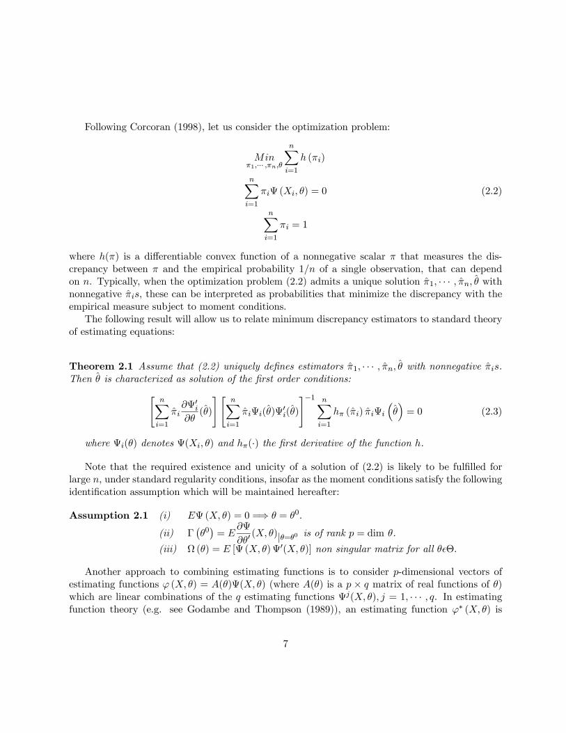
Following Corcoran (1998), let us consider the optimization problem:

Minπ1,··· ,πn,θ

nXi=1

h (πi)

nXi=1

πiΨ (Xi, θ) = 0 (2.2)

nXi=1

πi = 1

where h(π) is a differentiable convex function of a nonnegative scalar π that measures the dis-crepancy between π and the empirical probability 1/n of a single observation, that can dependon n. Typically, when the optimization problem (2.2) admits a unique solution π1, · · · , πn, θ withnonnegative πis, these can be interpreted as probabilities that minimize the discrepancy with theempirical measure subject to moment conditions.

The following result will allow us to relate minimum discrepancy estimators to standard theoryof estimating equations:

Theorem 2.1 Assume that (2.2) uniquely defines estimators π1, · · · , πn, θ with nonnegative πis.Then θ is characterized as solution of the first order conditions:"

nXi=1

πi∂Ψ0i∂θ(θ)

#"nXi=1

πiΨi(θ)Ψ0i(θ)

#−1 nXi=1

hπ (πi) πiΨi

³θ´= 0 (2.3)

where Ψi(θ) denotes Ψ(Xi, θ) and hπ(·) the first derivative of the function h.

Note that the required existence and unicity of a solution of (2.2) is likely to be fulfilled forlarge n, under standard regularity conditions, insofar as the moment conditions satisfy the followingidentification assumption which will be maintained hereafter:

Assumption 2.1 (i) EΨ (X, θ) = 0 =⇒ θ = θ0.

(ii) Γ¡θ0¢= E

∂Ψ

∂θ0(X, θ)|θ=θ0 is of rank p = dim θ.

(iii) Ω (θ) = E [Ψ (X, θ)Ψ0(X, θ)] non singular matrix for all θ²Θ.

Another approach to combining estimating functions is to consider p-dimensional vectors ofestimating functions ϕ (X, θ) = A(θ)Ψ(X, θ) (where A(θ) is a p × q matrix of real functions of θ)which are linear combinations of the q estimating functions Ψj(X, θ), j = 1, · · · , q. In estimatingfunction theory (e.g. see Godambe and Thompson (1989)), an estimating function ϕ∗ (X, θ) is

7

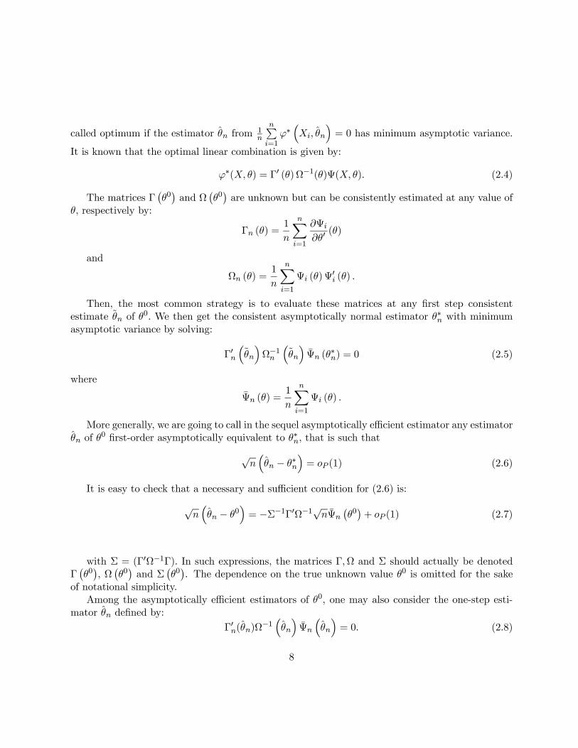
called optimum if the estimator θn from 1n

nPi=1

ϕ∗³Xi, θn

´= 0 has minimum asymptotic variance.

It is known that the optimal linear combination is given by:

ϕ∗(X, θ) = Γ0 (θ)Ω−1(θ)Ψ(X, θ). (2.4)

The matrices Γ¡θ0¢and Ω

¡θ0¢are unknown but can be consistently estimated at any value of

θ, respectively by:

Γn (θ) =1

n

nXi=1

∂Ψi∂θ0

(θ)

and

Ωn (θ) =1

n

nXi=1

Ψi (θ)Ψ0i (θ) .

Then, the most common strategy is to evaluate these matrices at any first step consistentestimate θn of θ0. We then get the consistent asymptotically normal estimator θ∗n with minimumasymptotic variance by solving:

Γ0n³θn

´Ω−1n

³θn

´Ψn (θ

∗n) = 0 (2.5)

where

Ψn (θ) =1

n

nXi=1

Ψi (θ) .

More generally, we are going to call in the sequel asymptotically efficient estimator any estimatorθn of θ0 first-order asymptotically equivalent to θ∗n, that is such that

√n³θn − θ∗n

´= oP (1) (2.6)

It is easy to check that a necessary and sufficient condition for (2.6) is:

√n³θn − θ0

´= −Σ−1Γ0Ω−1√nΨn

¡θ0¢+ oP (1) (2.7)

with Σ = (Γ0Ω−1Γ). In such expressions, the matrices Γ,Ω and Σ should actually be denotedΓ¡θ0¢, Ω

¡θ0¢and Σ

¡θ0¢. The dependence on the true unknown value θ0 is omitted for the sake

of notational simplicity.Among the asymptotically efficient estimators of θ0, one may also consider the one-step esti-

mator θn defined by:Γ0n(θn)Ω

−1³θn

´Ψn

³θn

´= 0. (2.8)

8

Although in general less computationally convenient than θ∗n, θn defined by (2.9) is worth com-paring to the minimum discrepancy estimators θ defined by theorem 2.1. One similarity and twodifferences are striking: In both cases, a left multiplication by a consistent estimator of the opti-mal selection matrix Γ0(θ0)Ω−1

¡θ0¢is applied to some weighting average of the sample estimating

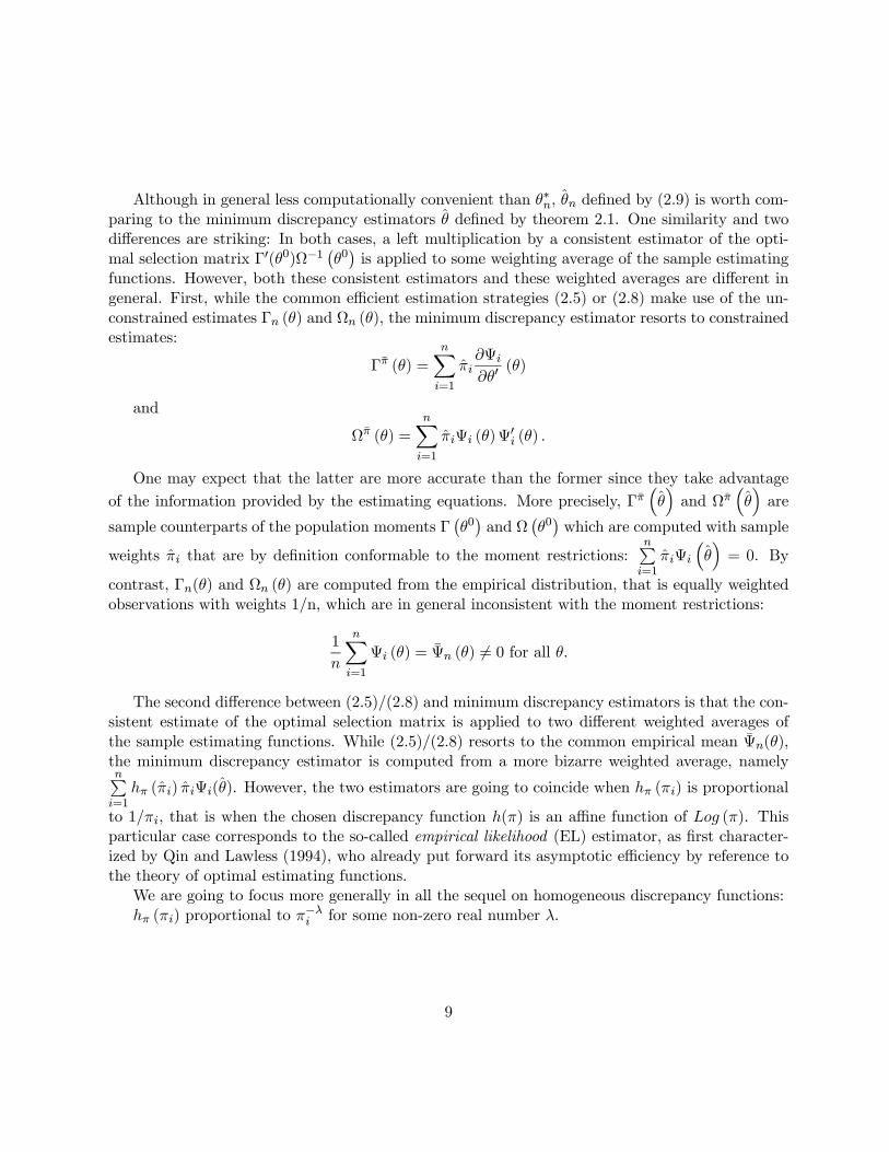
functions. However, both these consistent estimators and these weighted averages are different ingeneral. First, while the common efficient estimation strategies (2.5) or (2.8) make use of the un-constrained estimates Γn (θ) and Ωn (θ), the minimum discrepancy estimator resorts to constrainedestimates:

Γπ (θ) =nXi=1

πi∂Ψi∂θ0

(θ)

and

Ωπ (θ) =nXi=1

πiΨi (θ)Ψ0i (θ) .

One may expect that the latter are more accurate than the former since they take advantageof the information provided by the estimating equations. More precisely, Γπ

³θ´and Ωπ

³θ´are

sample counterparts of the population moments Γ¡θ0¢and Ω

¡θ0¢which are computed with sample

weights πi that are by definition conformable to the moment restrictions:nPi=1

πiΨi

³θ´= 0. By

contrast, Γn(θ) and Ωn (θ) are computed from the empirical distribution, that is equally weightedobservations with weights 1/n, which are in general inconsistent with the moment restrictions:

1

n

nXi=1

Ψi (θ) = Ψn (θ) 6= 0 for all θ.

The second difference between (2.5)/(2.8) and minimum discrepancy estimators is that the con-sistent estimate of the optimal selection matrix is applied to two different weighted averages ofthe sample estimating functions. While (2.5)/(2.8) resorts to the common empirical mean Ψn(θ),the minimum discrepancy estimator is computed from a more bizarre weighted average, namelynPi=1hπ (πi) πiΨi(θ). However, the two estimators are going to coincide when hπ (πi) is proportional

to 1/πi, that is when the chosen discrepancy function h(π) is an affine function of Log (π). Thisparticular case corresponds to the so-called empirical likelihood (EL) estimator, as first character-ized by Qin and Lawless (1994), who already put forward its asymptotic efficiency by reference tothe theory of optimal estimating functions.

We are going to focus more generally in all the sequel on homogeneous discrepancy functions:hπ (πi) proportional to π−λi for some non-zero real number λ.

9

2.2 Implied probabilities associated to power—divergence statistics

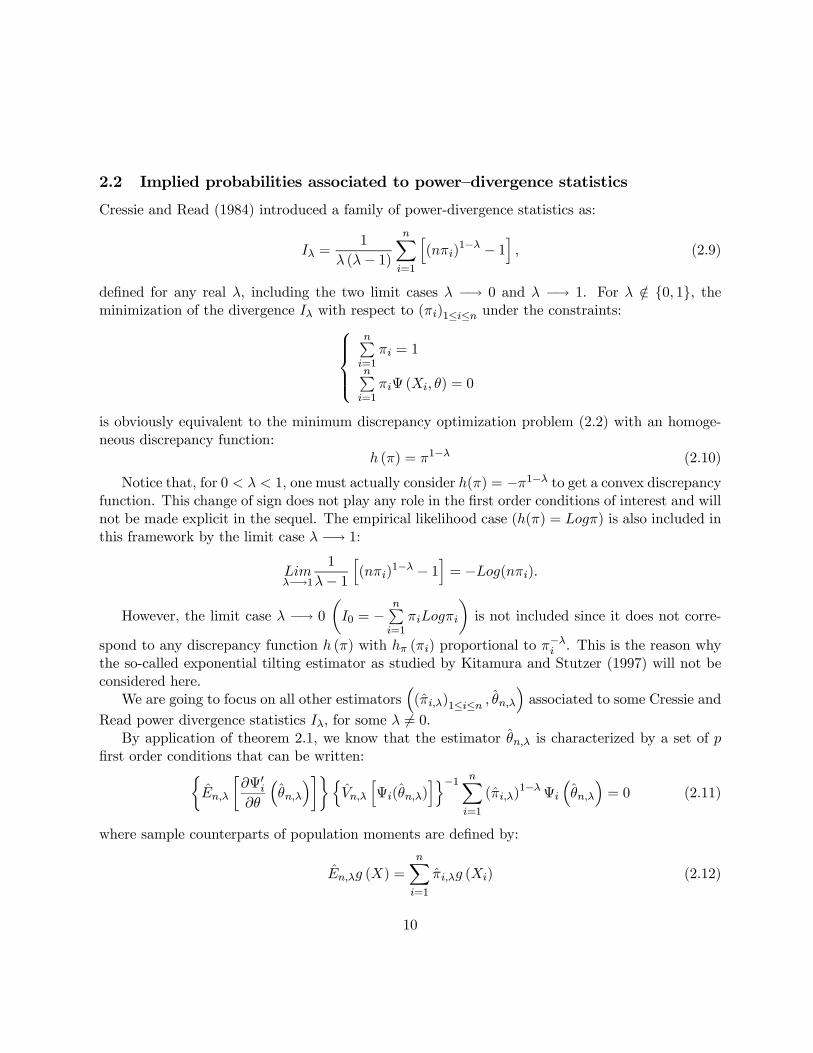
Cressie and Read (1984) introduced a family of power-divergence statistics as:

Iλ =1

λ (λ− 1)nXi=1

h(nπi)

1−λ − 1i, (2.9)

defined for any real λ, including the two limit cases λ −→ 0 and λ −→ 1. For λ /∈ 0, 1, theminimization of the divergence Iλ with respect to (πi)1≤i≤n under the constraints:

nPi=1

πi = 1

nPi=1

πiΨ (Xi, θ) = 0

is obviously equivalent to the minimum discrepancy optimization problem (2.2) with an homoge-neous discrepancy function:

h (π) = π1−λ (2.10)

Notice that, for 0 < λ < 1, one must actually consider h(π) = −π1−λ to get a convex discrepancyfunction. This change of sign does not play any role in the first order conditions of interest and willnot be made explicit in the sequel. The empirical likelihood case (h(π) = Logπ) is also included inthis framework by the limit case λ −→ 1:

Limλ−→1

1

λ− 1h(nπi)

1−λ − 1i= −Log(nπi).

However, the limit case λ −→ 0

µI0 = −

nPi=1

πiLogπi

¶is not included since it does not corre-

spond to any discrepancy function h (π) with hπ (πi) proportional to π−λi . This is the reason whythe so-called exponential tilting estimator as studied by Kitamura and Stutzer (1997) will not beconsidered here.

We are going to focus on all other estimators³(πi,λ)1≤i≤n , θn,λ

´associated to some Cressie and

Read power divergence statistics Iλ, for some λ 6= 0.By application of theorem 2.1, we know that the estimator θn,λ is characterized by a set of p

first order conditions that can be written:½En,λ

·∂Ψ0i∂θ

³θn,λ

´¸¾nVn,λ

hΨi(θn,λ)

io−1 nXi=1

(πi,λ)1−λΨi

³θn,λ

´= 0 (2.11)

where sample counterparts of population moments are defined by:

En,λg (X) =nXi=1

πi,λg (Xi) (2.12)

10

Vn,λg (X) =nXi=1

πi,λ

hg (Xi)− En,λg(X)

ig0 (Xi) .

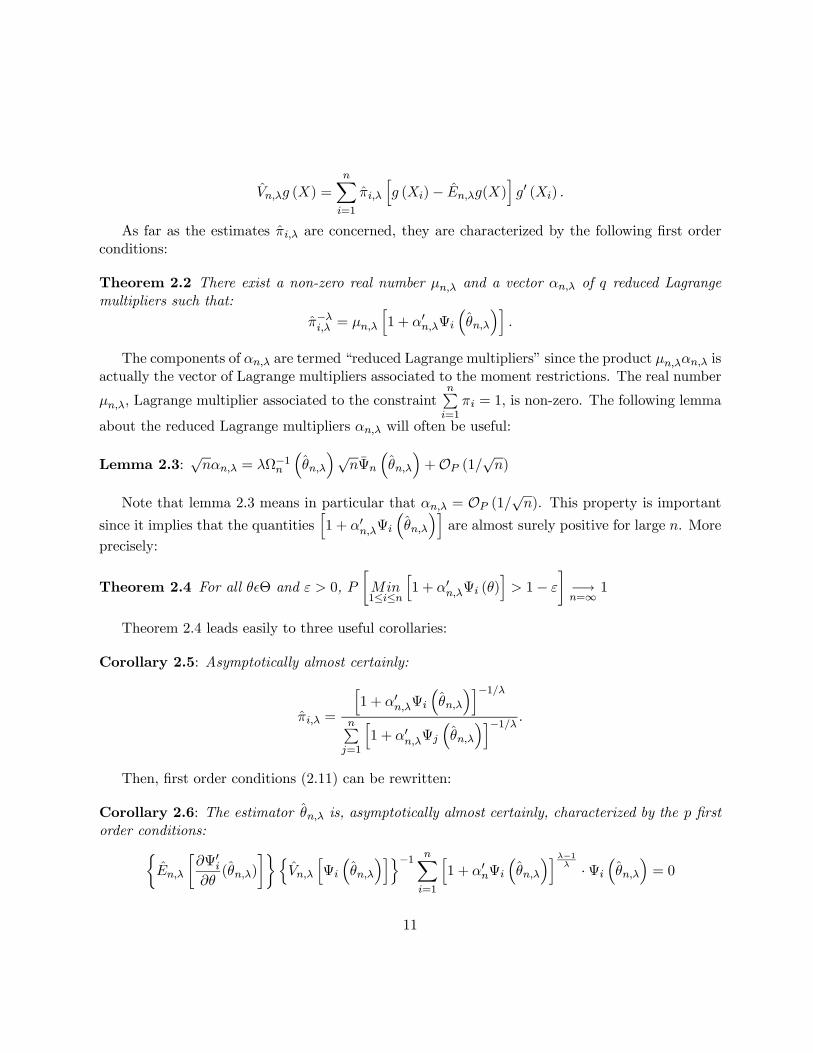
As far as the estimates πi,λ are concerned, they are characterized by the following first orderconditions:

Theorem 2.2 There exist a non-zero real number µn,λ and a vector αn,λ of q reduced Lagrangemultipliers such that:

π−λi,λ = µn,λh1 + α0n,λΨi

³θn,λ

í.

The components of αn,λ are termed “reduced Lagrange multipliers” since the product µn,λαn,λ isactually the vector of Lagrange multipliers associated to the moment restrictions. The real number

µn,λ, Lagrange multiplier associated to the constraintnPi=1

πi = 1, is non-zero. The following lemma

about the reduced Lagrange multipliers αn,λ will often be useful:

Lemma 2.3:√nαn,λ = λΩ−1n

³θn,λ

´√nΨn

³θn,λ

´+OP (1/

√n)

Note that lemma 2.3 means in particular that αn,λ = OP (1/√n). This property is important

since it implies that the quantitiesh1 + α0n,λΨi

³θn,λ

íare almost surely positive for large n. More

precisely:

Theorem 2.4 For all θ²Θ and ε > 0, P·Min1≤i≤n

h1 + α0n,λΨi (θ)

i> 1− ε

¸−→n=∞ 1

Theorem 2.4 leads easily to three useful corollaries:

Corollary 2.5: Asymptotically almost certainly:

πi,λ =

h1 + α0n,λΨi

³θn,λ

í−1/λnPj=1

h1 + α0n,λΨj

³θn,λ

í−1/λ .Then, first order conditions (2.11) can be rewritten:

Corollary 2.6: The estimator θn,λ is, asymptotically almost certainly, characterized by the p firstorder conditions:½

En,λ

·∂Ψ0i∂θ(θn,λ)

¸¾nVn,λ

hΨi

³θn,λ

ío−1 nXi=1

h1 + α0nΨi

³θn,λ

íλ−1λ ·Ψi

³θn,λ

´= 0

11

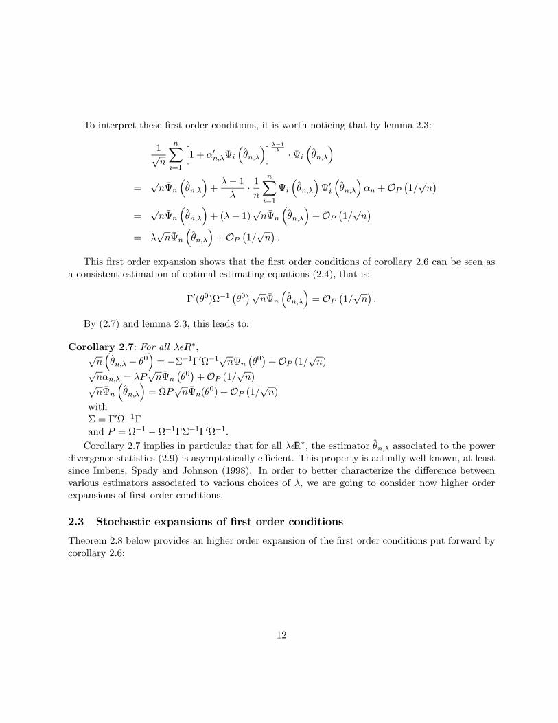
To interpret these first order conditions, it is worth noticing that by lemma 2.3:

1√n

nXi=1

h1 + α0n,λΨi

³θn,λ

´iλ−1λ ·Ψi

³θn,λ

´=√nΨn

³θn,λ

´+

λ− 1λ

· 1n

nXi=1

Ψi

³θn,λ

´Ψ0i³θn,λ

´αn +OP

¡1/√n¢

=√nΨn

³θn,λ

´+ (λ− 1)√nΨn

³θn,λ

´+OP

¡1/√n¢

= λ√nΨn

³θn,λ

´+OP

¡1/√n¢.

This first order expansion shows that the first order conditions of corollary 2.6 can be seen asa consistent estimation of optimal estimating equations (2.4), that is:

Γ0(θ0)Ω−1¡θ0¢√nΨn

³θn,λ

´= OP

¡1/√n¢.

By (2.7) and lemma 2.3, this leads to:

Corollary 2.7: For all λ²IR∗,√n³θn,λ − θ0

´= −Σ−1Γ0Ω−1√nΨn

¡θ0¢+OP (1/

√n)√

nαn,λ = λP√nΨn

¡θ0¢+OP (1/

√n)√

nΨn

³θn,λ

´= ΩP

√nΨn(θ

0) +OP (1/√n)

withΣ = Γ0Ω−1Γand P = Ω−1 − Ω−1ΓΣ−1Γ0Ω−1.Corollary 2.7 implies in particular that for all λ²IR∗, the estimator θn,λ associated to the power

divergence statistics (2.9) is asymptotically efficient. This property is actually well known, at leastsince Imbens, Spady and Johnson (1998). In order to better characterize the difference betweenvarious estimators associated to various choices of λ, we are going to consider now higher orderexpansions of first order conditions.

2.3 Stochastic expansions of first order conditions

Theorem 2.8 below provides an higher order expansion of the first order conditions put forward bycorollary 2.6:

12

Theorem 2.8

1√n

nXi=1

h1 + α0n,λΨi

³θn,λ

´iλ−1λΨi(θn,λ)

= λ√nΨn

³θn,λ

´+

λ(λ− 1)2

1√n

qXj=1

βjn(θ0)ej +OP (1/n)

where for j = 1, · · · , q, ej denotes the q-dimensional vector with all coefficients equal to zero,except the jth one equal to one, and:

βjn(θ0) =

√nΨ0n

¡θ0¢P 0E

£Ψ(X, θ0)Ψ0

¡X, θ0

¢Ψj¡X, θ0

¢¤P√nΨn

¡θ0¢= OP (1)

In other words, for all λ 6= 0, θn,λ is defined by first order conditions stochastically expandedas: ½

En,λ∂Ψ0i∂θ(θn,λ)

¾nVn,λ

hΨi(θn,λ)

io−1√nΨn ³θn,λ´+ λ− 12√n

qXj=1

βjn(θ0)ej

= OP (1/n)

(2.13)It means that, up to some OP (1/n), the first order conditions defining θn,λ are different from

the ones of empirical likelihood (case λ = 1) when the random variableqPj=1

βjn(θ0)ej is not zero in

probability.Note that each βjn(θ

0), j = 1, · · · , q, is asymptotically a quadratic form on a standardizedGaussian vector of dimension q: Tn

¡θ0¢= Ω−1/2

¡θ0¢√nΨn(θ

0). This quadratic form is zero ifand only if:

E£Ψ(X, θ0)Ψ0

¡X, θ0

¢Ψj¡X, θ0

¢¤P = 0.

This condition is fulfilled in particular when third moments of Ψ¡X, θ0

¢are zero:

EhΨj¡X, θ0

¢Ψk(X, θ0)Ψl(X, θ0)

i= 0 for j, k, l = 1, · · · , q. (2.14)

As noticed by Newey and Smith (2004), this third moment condition will hold in an IV setting,when disturbances are symmetrically distributed. More precisely, Newey and Smith (2004) (seetheir theorem 4.1 and their comments after corollary 4.4) state that:

First, the higher order bias of θn,λ with respect to empirical likelihood is zero when:

E£Ψ¡X, θ0

¢Ψ0¡X, θ0

¢PΨ

¡X, θ0

¢¤= 0. (2.15)

Second, when the zero third moments condition holds, one can actually show the stronger resultthat:

θn,λ − θn,1 = OP³n−3/2

´. (2.16)

13

This stronger result will be shown in section 3 below to be a corollary of theorem 2.8 when theβjn

¡θ0¢, j = 1, · · · , q are all zero, that is:

E£Ψ¡X, θ0

¢Ψ0¡X, θ0

¢PΨj

¡X, θ0

¢¤= 0 for j = 1, · · · , q (2.17)

Note that this condition, although possibly slightly weaker than the zero third moments condi-tion, is actually stronger than the Newey and Smith’s zero-bias condition (2.15).

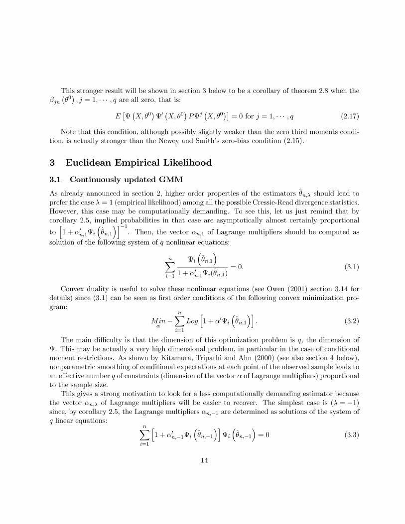
3 Euclidean Empirical Likelihood

3.1 Continuously updated GMM

As already announced in section 2, higher order properties of the estimators θn,λ should lead toprefer the case λ = 1 (empirical likelihood) among all the possible Cressie-Read divergence statistics.However, this case may be computationally demanding. To see this, let us just remind that bycorollary 2.5, implied probabilities in that case are asymptotically almost certainly proportional

toh1 + α0n,1Ψi

³θn,1

í−1. Then, the vector αn,1 of Lagrange multipliers should be computed as

solution of the following system of q nonlinear equations:

nXi=1

Ψi

³θn,1

´1 + α0n,1Ψi(θn,1)

= 0. (3.1)

Convex duality is useful to solve these nonlinear equations (see Owen (2001) section 3.14 fordetails) since (3.1) can be seen as first order conditions of the following convex minimization pro-gram:

Minα−

nXi=1

Logh1 + α0Ψi

³θn,1

í. (3.2)

The main difficulty is that the dimension of this optimization problem is q, the dimension ofΨ. This may be actually a very high dimensional problem, in particular in the case of conditionalmoment restrictions. As shown by Kitamura, Tripathi and Ahn (2000) (see also section 4 below),nonparametric smoothing of conditional expectations at each point of the observed sample leads toan effective number q of constraints (dimension of the vector α of Lagrange multipliers) proportionalto the sample size.

This gives a strong motivation to look for a less computationally demanding estimator becausethe vector αn,λ of Lagrange multipliers will be easier to recover. The simplest case is (λ = −1)since, by corollary 2.5, the Lagrange multipliers αn,−1 are determined as solutions of the system ofq linear equations:

nXi=1

h1 + α0n,−1Ψi

³θn,−1

íΨi

³θn,−1

´= 0 (3.3)

14

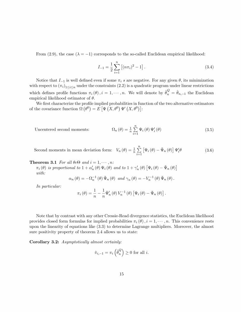
From (2.9), the case (λ = −1) corresponds to the so-called Euclidean empirical likelihood:

I−1 =1

2

nXi=1

£(nπi)

2 − 1¤ . (3.4)

Notice that I−1 is well defined even if some πi s are negative. For any given θ, its minimizationwith respect to (πi)1≤i≤n under the constraints (2.2) is a quadratic program under linear restrictions

which defines profile functions πi (θ) , i = 1, · · · , n. We will denote by θQn = θn,−1 the Euclidean

empirical likelihood estimator of θ.We first characterize the profile implied probabilities in function of the two alternative estimators

of the covariance function Ω¡θ0¢= E

£Ψ¡X, θ0

¢Ψ0¡X, θ0

¢¤:

Uncentered second moments: Ωn (θ) =1n

nPi=1Ψi (θ)Ψ

0i (θ) (3.5)

Second moments in mean deviation form: Vn (θ) =1n

nPi=1

£Ψi (θ)− Ψn (θ)

¤Ψ0iθ (3.6)

Theorem 3.1 For all θ²Θ and i = 1, · · · , n:πi (θ) is proportional to 1 + α0n (θ)Ψi (θ) and to 1 + γ0n (θ)


¤with:

αn (θ) = −Ω−1n (θ) Ψn (θ) and γn (θ) = −V −1n (θ) Ψn (θ) .

In particular:

πi (θ) =1

n− 1nΨ0n (θ)V

−1n (θ)


¤.

Note that by contrast with any other Cressie-Read divergence statistics, the Euclidean likelihoodprovides closed form formulas for implied probabilities πi (θ) , i = 1, · · · , n. This convenience restsupon the linearity of equations like (3.3) to determine Lagrange multipliers. Moreover, the almostsure positivity property of theorem 2.4 allows us to state:

Corollary 3.2: Asymptotically almost certainly:

πi,−1 = πi

³θQn

´≥ 0 for all i.

15

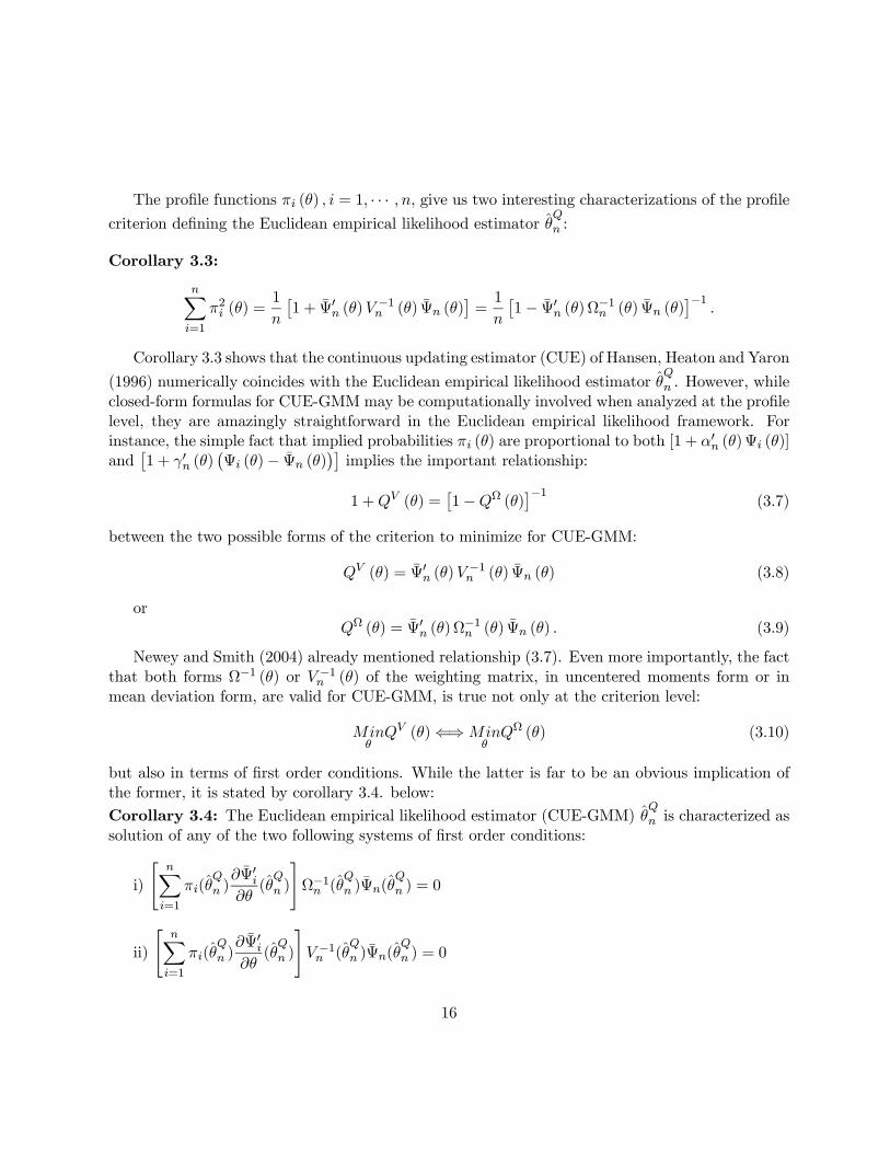
The profile functions πi (θ) , i = 1, · · · , n, give us two interesting characterizations of the profilecriterion defining the Euclidean empirical likelihood estimator θ

Qn :

Corollary 3.3:

nXi=1

π2i (θ) =1

n

£1 + Ψ0n (θ)V

−1n (θ) Ψn (θ)

¤=1

n

£1− Ψ0n (θ)Ω−1n (θ) Ψn (θ)

¤−1.

Corollary 3.3 shows that the continuous updating estimator (CUE) of Hansen, Heaton and Yaron

(1996) numerically coincides with the Euclidean empirical likelihood estimator θQn . However, while

closed-form formulas for CUE-GMM may be computationally involved when analyzed at the profilelevel, they are amazingly straightforward in the Euclidean empirical likelihood framework. Forinstance, the simple fact that implied probabilities πi (θ) are proportional to both [1 + α0n (θ)Ψi (θ)]and

£1 + γ0n (θ)

¡Ψi (θ)− Ψn (θ)

¢¤implies the important relationship:

1 +QV (θ) =£1−QΩ (θ)

¤−1(3.7)

between the two possible forms of the criterion to minimize for CUE-GMM:

QV (θ) = Ψ0n (θ)V−1n (θ) Ψn (θ) (3.8)

orQΩ (θ) = Ψ0n (θ)Ω

−1n (θ) Ψn (θ) . (3.9)

Newey and Smith (2004) already mentioned relationship (3.7). Even more importantly, the factthat both forms Ω−1 (θ) or V −1n (θ) of the weighting matrix, in uncentered moments form or inmean deviation form, are valid for CUE-GMM, is true not only at the criterion level:

MinθQV (θ)⇐⇒Min

θQΩ (θ) (3.10)

but also in terms of first order conditions. While the latter is far to be an obvious implication ofthe former, it is stated by corollary 3.4. below:

Corollary 3.4: The Euclidean empirical likelihood estimator (CUE-GMM) θQn is characterized as

solution of any of the two following systems of first order conditions:

i)

"nXi=1

πi(θQn )

∂Ψ0i∂θ(θQn )

#Ω−1n (θ

Qn )Ψn(θ

Qn ) = 0

ii)

"nXi=1

πi(θQn )

∂Ψ0i∂θ(θQn )

#V −1n (θ

Qn )Ψn(θ

Qn ) = 0

16

Corollary 3.4 is still a straightforward implication of the two possible forms αn (θ) and γn (θ)of the vector of reduced Lagrange multipliers. Newey and Smith (2004), theorem 2.3, put forwardthe first form of these first order conditions. In comparing the empirical likelihood first orderconditions ((2.11) with λ = 1) and CUE-GMM first order conditions, they stress that, while bothuse the relevant constrained estimator of the Jacobian matrix Γ

¡θ0¢by taking into account implied

probabilities πi,λ, CUE-GMM has the drawback to use an unconstrained estimator of the weightingmatrix Ω

¡θ0¢. This criticism may however be mitigated in two respects:

First, as shown by (2.13), the difference between the two estimators can be interpreted in adifferent way, where the weighting matrix is well-estimated in both cases, but symmetry propertiesof the moment conditions are at stake.

Second, the form (ii) of first order conditions in corollary 3.4 shows that the weighting matrixestimator may be seen in its mean deviation form. It is important to stress that this is a secondadvantage, besides the estimation of the Jacobian matrix, of CUE-GMM with respect to commonuse of two-stage GMM (2S-GMM).

Two-stage GMM is actually defined, since Hansen (1982), as the minimization over θ of:

Q∗Ω (θ) = Ψ0n (θ)Ω−1n

³θn

´Ψn (θ) (3.11)

for a given consistent first step estimator θn of θ.However, Hall (2000) argues that the mean deviation form should be preferred, leading to the

minimization over θ of:Q∗V (θ) = Ψ0n (θ)V

−1n

³θn

´Ψn (θ) (3.12)

First order conditions associated to (3.11) define a two-step GMM estimator θ2SΩn as solution

of:∂Ψ0n∂θ

³θ2SΩn

´Ω−1n

³θn

´Ψn

³θ2SΩn

´= 0. (3.13)

Another two-step GMM estimator θ2SVn is defined by the first order conditions of (3.12):

∂Ψ0n∂θ

³θ2SVn

´V −1n

³θn

´Ψn

³θ2SV

´= 0. (3.14)

It is worth realizing that, by contrast with corollary 3.4, there is no reason to imagine that

equations (3.13) and (3.14) are equivalent. In other words, the common 2S-GMM estimator θ2SGn

should have less nice properties than CUE-GMM not only because it uses more biased estimatorof the Jacobian matrix but also because it does not use the estimator of the covariance matrixin its mean deviation form. By contrast, the 2S-GMM estimator in mean deviation form θ

2SVn is

expected to have better properties and actually coincides with CUE-GMM in the particular caseof separable moment conditions:

Ψ (X, θ) = ϕ(X)− k(θ). (3.15)

17

Notice that in such a case, there is no issue of estimation of the Jacobian matrix. As far as thebias in the estimation of this matrix is concerned for more general moment conditions, it is worth

interpreting the constrained estimatornPi=1

πi

³θQn

´∂Ψi∂θ0

³θQn

úsed by CUE-GMM (see corollary 3.4)

in the light of corollary 3.5 below:

Corollary 3.5: For any integrable real function g(X), Eg(X) can be estimated by:

gn

³θQn

´=

nXi=1

πi

³θQn

´g(Xi)

= gn − Covnhg(Xi),Ψi(θ

Qn )i hVn

³θQn

í−1Ψn(θ

Qn )

where:

gn =1

n

nXi=1

g (Xi)

Covn

hg(Xi),Ψi(θ

Qn )i=

1

n

nXi=1

[g (Xi)− gn]Ψ0i(θQn )

The intuition behind the estimator gn³θQn

ís very clear. If we knew the true value θ0 of θ, we

would get an unbiased estimator of Eg (X) by considering gn−a0Ψn¡θ0¢for any given q-dimensional

vector a. The minimum variance estimator is obtained for:

a = Cov£g (X) ,Ψ

¡X, θ0

¢¤ ¡V ar

£Ψ¡X, θ0

¢¤¢−1(3.16)

and it will be made feasible by replacing a by its sample counterpart:

an = Covn£g (Xi) ,Ψi

¡θ0¢¤ £Vn¡θ0¢¤−1

. (3.17)

This is nothing but the well known principle of control variates as defined for instance by Fieller

and Hartley (1954). Moreover, since we don’t know the true value θ0, the estimator gn³θQn

´just

proposes an extension of the control variates principle where θ0 is replaced by θQn . In this respect,

the choice of Euclidean empirical likelihood to estimate the implied probability distribution appearsto be fairly conformable to classical strategies for survey sampling or Monte Carlo experiments.The above control variates interpretation complements the jackknife interpretation of CUE-GMMproposed by Donald and Newey (2000).

18

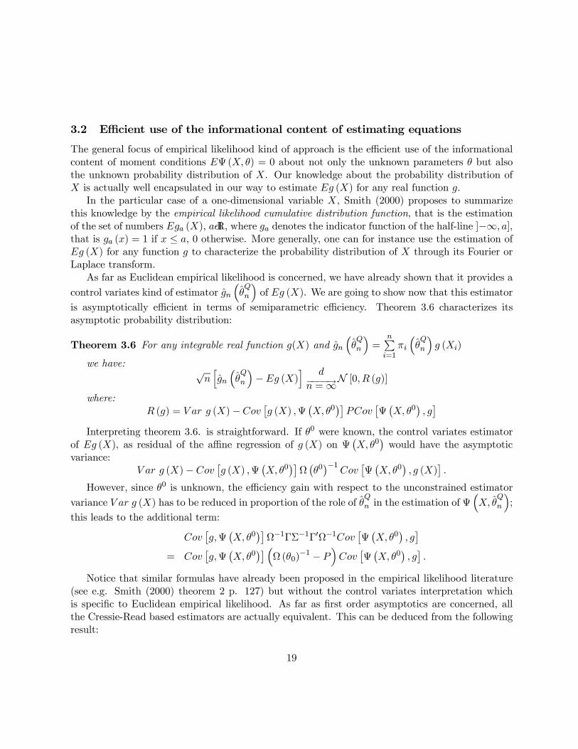
3.2 Efficient use of the informational content of estimating equations

The general focus of empirical likelihood kind of approach is the efficient use of the informationalcontent of moment conditions EΨ (X, θ) = 0 about not only the unknown parameters θ but alsothe unknown probability distribution of X. Our knowledge about the probability distribution ofX is actually well encapsulated in our way to estimate Eg (X) for any real function g.

In the particular case of a one-dimensional variable X, Smith (2000) proposes to summarizethis knowledge by the empirical likelihood cumulative distribution function, that is the estimationof the set of numbers Ega (X), a²IR, where ga denotes the indicator function of the half-line ]−∞, a],that is ga (x) = 1 if x ≤ a, 0 otherwise. More generally, one can for instance use the estimation ofEg (X) for any function g to characterize the probability distribution of X through its Fourier orLaplace transform.

As far as Euclidean empirical likelihood is concerned, we have already shown that it provides a

control variates kind of estimator gn³θQn

´of Eg (X). We are going to show now that this estimator

is asymptotically efficient in terms of semiparametric efficiency. Theorem 3.6 characterizes itsasymptotic probability distribution:

Theorem 3.6 For any integrable real function g(X) and gn³θQn

´=

nPi=1

πi

³θQn

´g (Xi)

we have: √nhgn

³θQn

´−Eg (X)

i d−−−−→n =∞N [0, R (g)]

where:R (g) = V ar g (X)−Cov £g (X) ,Ψ ¡X, θ0¢¤PCov £Ψ ¡X, θ0¢ , g¤

Interpreting theorem 3.6. is straightforward. If θ0 were known, the control variates estimatorof Eg (X), as residual of the affine regression of g (X) on Ψ

¡X, θ0

¢would have the asymptotic

variance:V ar g (X)− Cov £g (X) ,Ψ ¡X, θ0¢¤Ω ¡θ0¢−1Cov £Ψ ¡X, θ0¢ , g (X)¤ .

However, since θ0 is unknown, the efficiency gain with respect to the unconstrained estimator

variance V ar g (X) has to be reduced in proportion of the role of θQn in the estimation of Ψ

³X, θ

Qn

´;

this leads to the additional term:

Cov£g,Ψ

¡X, θ0

¢¤Ω−1ΓΣ−1Γ0Ω−1Cov

£Ψ¡X, θ0

¢, g¤

= Cov£g,Ψ

¡X, θ0

¢¤ ³Ω (θ0)

−1 − P´Cov

£Ψ¡X, θ0

¢, g¤.

Notice that similar formulas have already been proposed in the empirical likelihood literature(see e.g. Smith (2000) theorem 2 p. 127) but without the control variates interpretation whichis specific to Euclidean empirical likelihood. As far as first order asymptotics are concerned, allthe Cressie-Read based estimators are actually equivalent. This can be deduced from the followingresult:

19

Theorem 3.7 Let³πi,λ, i = 1, · · · , n, θn,λ

´denote the estimator associated to the power divergence

statistics Iλ,λ 6= 0, and some moment conditions EΨ (X, θ) = 0. Define the augmented set of

moment conditions: EΨ˜

µX, θ

˜

¶= 0, where:

θ˜

= (θ0, ξ)0

Ψ˜

µX, θ

˜

¶=

¡Ψ0 (X, θ) , g(X)− ξ

¢for some real integrable function g.

Letµπ˜ i,λ, i = 1 · · ·n, θ

˜n,λ

¶the estimator associated to Iλ and the augmented set of moment

conditions. Then:

π˜ i,λ

= πi,λ for i = 1, · · ·n

θ˜n,λ

=³θ0n,λ, ξn,λ

´0with

ξn,λ =nXi=1

πi,λ g(Xi) = En,λg (X)

Theorem 3.7 ensures some internal consistency to the estimation approach and, from corollary2.7, implies the first order asymptotic equivalence of the various estimators of g (X):

Corollary 3.8: For all λ 6= 0√n³En,λg(X)− gn(θQn )

´= oP (1)

Moreover, the Euclidean likelihood based interpretation of CUE-GMM leads to:

Corollary 3.9: With the notations of theorem 3.7:

ξQn =

nXi=1

πi

³θQn

´g (Xi) = gn(θ

Qn )

corresponds to the CUE-GMM estimator θ˜

Q

n=³θQ0n , ξ

Qn

´0defined by the augmented set of

moment conditions EΨ˜

µX, θ

˜

¶= 0.

It is worth reminding that Back and Brown (1993) had already derived a similar result inthe context of 2S-GMM. However, the framework of Euclidean empirical likelihood makes the

20

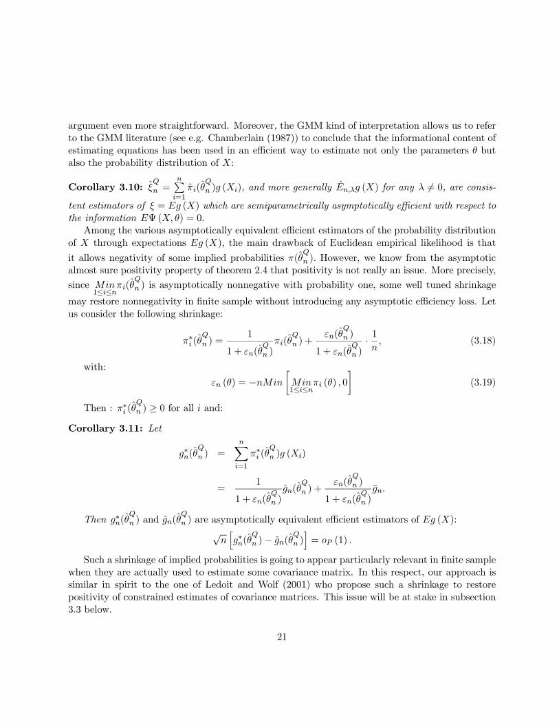
argument even more straightforward. Moreover, the GMM kind of interpretation allows us to referto the GMM literature (see e.g. Chamberlain (1987)) to conclude that the informational content ofestimating equations has been used in an efficient way to estimate not only the parameters θ butalso the probability distribution of X:

Corollary 3.10: ξQn =

nPi=1

πi(θQn )g (Xi), and more generally En,λg (X) for any λ 6= 0, are consis-

tent estimators of ξ = Eg (X) which are semiparametrically asymptotically efficient with respect tothe information EΨ (X, θ) = 0.

Among the various asymptotically equivalent efficient estimators of the probability distributionof X through expectations Eg (X), the main drawback of Euclidean empirical likelihood is that

it allows negativity of some implied probabilities π(θQn ). However, we know from the asymptotic

almost sure positivity property of theorem 2.4 that positivity is not really an issue. More precisely,

since Min1≤i≤n

πi(θQn ) is asymptotically nonnegative with probability one, some well tuned shrinkage

may restore nonnegativity in finite sample without introducing any asymptotic efficiency loss. Letus consider the following shrinkage:

π∗i (θQn ) =

1

1 + εn(θQn )

πi(θQn ) +

εn(θQn )

1 + εn(θQn )· 1n, (3.18)

with:

εn (θ) = −nMin·Min1≤i≤n

πi (θ) , 0

¸(3.19)

Then : π∗i (θQn ) ≥ 0 for all i and:

Corollary 3.11: Let

g∗n(θQn ) =

nXi=1

π∗i (θQn )g (Xi)

=1

1 + εn(θQn )gn(θ

Qn ) +

εn(θQn )

1 + εn(θQn )gn.

Then g∗n(θQn ) and gn(θ

Qn ) are asymptotically equivalent efficient estimators of Eg (X):

√nhg∗n(θ

Qn )− gn(θ

Qn )i= oP (1) .

Such a shrinkage of implied probabilities is going to appear particularly relevant in finite samplewhen they are actually used to estimate some covariance matrix. In this respect, our approach issimilar in spirit to the one of Ledoit and Wolf (2001) who propose such a shrinkage to restorepositivity of constrained estimates of covariance matrices. This issue will be at stake in subsection3.3 below.

21

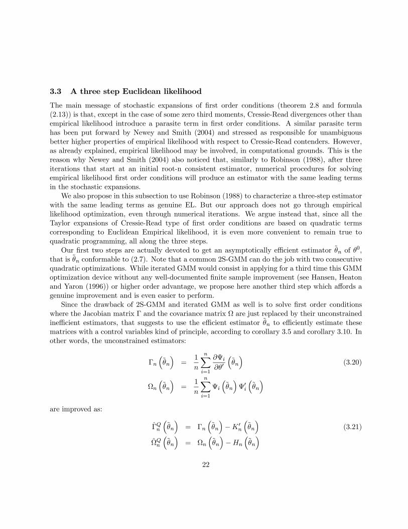
3.3 A three step Euclidean likelihood

The main message of stochastic expansions of first order conditions (theorem 2.8 and formula(2.13)) is that, except in the case of some zero third moments, Cressie-Read divergences other thanempirical likelihood introduce a parasite term in first order conditions. A similar parasite termhas been put forward by Newey and Smith (2004) and stressed as responsible for unambiguousbetter higher properties of empirical likelihood with respect to Cressie-Read contenders. However,as already explained, empirical likelihood may be involved, in computational grounds. This is thereason why Newey and Smith (2004) also noticed that, similarly to Robinson (1988), after threeiterations that start at an initial root-n consistent estimator, numerical procedures for solvingempirical likelihood first order conditions will produce an estimator with the same leading termsin the stochastic expansions.

We also propose in this subsection to use Robinson (1988) to characterize a three-step estimatorwith the same leading terms as genuine EL. But our approach does not go through empiricallikelihood optimization, even through numerical iterations. We argue instead that, since all theTaylor expansions of Cressie-Read type of first order conditions are based on quadratic termscorresponding to Euclidean Empirical likelihood, it is even more convenient to remain true toquadratic programming, all along the three steps.

Our first two steps are actually devoted to get an asymptotically efficient estimator θn of θ0,that is θn conformable to (2.7). Note that a common 2S-GMM can do the job with two consecutivequadratic optimizations. While iterated GMM would consist in applying for a third time this GMMoptimization device without any well-documented finite sample improvement (see Hansen, Heatonand Yaron (1996)) or higher order advantage, we propose here another third step which affords agenuine improvement and is even easier to perform.

Since the drawback of 2S-GMM and iterated GMM as well is to solve first order conditionswhere the Jacobian matrix Γ and the covariance matrix Ω are just replaced by their unconstrainedinefficient estimators, that suggests to use the efficient estimator θn to efficiently estimate thesematrices with a control variables kind of principle, according to corollary 3.5 and corollary 3.10. Inother words, the unconstrained estimators:

Γn

³θn

´=

1

n

nXi=1

∂Ψi∂θ0

³θn

´(3.20)

Ωn

³θn

´=

1

n

nXi=1

Ψi

³θn

´Ψ0i³θn

´are improved as:

ΓQn

³θn

´= Γn

³θn

´−K 0

n

³θn

´(3.21)

ΩQn

³θn

´= Ωn

³θn

´−Hn

³θn

´22

where the jth columns, j = 1, · · · , q of the matrices Kn³θn

ánd Hn

³θn

áre respectively defined

by:

Kjn

³θn

´= Covn

"∂Ψji∂θ

³θn

´,Ψi

³θn

´# hVn

³θn

í−1Ψn

³θn

´(3.22)

andHjn

³θn

´= Covn

hΨi

³θn

´Ψji

³θn

´,Ψi

³θn

í hVn

³θn

í−1Ψn

³θn

´.

Notice that, as confirmed by theorem 3.12 below, this improvement in the estimation of the jth

column of the matrix Ω¡θ0¢would be useless if:

CovhΨi¡θ0¢Ψji¡θ0¢,Ψi

¡θ0¢i= E

hΨi¡θ0¢Ψ0i¡θ0¢Ψji¡θ0¢i= 0 (3.23)

This actually confirms the intuition provided by stochastic expansions of first order conditionsin theorem 2.8 and formula (2.13). While CUE-GMM shares with 2S-GMM the drawback of abiased estimator of the covariance matrix used in first order conditions (see corollary 3.4), thisbias vanishes when third moments are zero as in (3.23). The deep reason for this higher orderequivalence between CUE-GMM and empirical likelihood with kind of symmetric errors is that, inthat case, the control variables principle based on the information “EΨ

¡X, θ0

¢= 0” does not allow

to improve the estimation of the covariance matrix; the cross-product terms Ψj¡X, θ0

¢Ψl¡X, θ0

¢the expectation of which defines the covariance matrix are actually uncorellated with the randomvector Ψ

¡X, θ0

¢.

On the contrary, when the zero third moment conditions is not fulfilled, our control variatesimprovement of Ωn(θn) by Ω

Qn (θn) is exactly what is needed to protect against the bias of 2S-

GMM well-documented in small samples. For example, in a simulation study, Altonji and Segal(1996) demonstrated that “the bias arises because sampling errors in the moments are correlatedwith sampling errors in the estimate of the covariance matrix of the sample moments”. Since ΩQnand ΓQn are defined from residuals of affine regressions on the moments of interest, such perversecorrelations have precisely been deleted. As far as higher order equivalence between empiricallikelihood and a suitably corrected quadratic procedure is concerned, it will be obtained thanks tothe following result:

Theorem 3.12 Let θn be an asymptotically efficient estimator of θ0:

θn − θn,λ = Op (1/n) for all λ 6= 0.Let θn defined as solution of p equations:

ΓQ0n³θn

´ hΩQn

³θn

í−1Ψn

³θn

´= OP

¡1/n√n¢.

Thenθn − θn,1 = OP

¡1/n√n¢.

23

In other words, the third step estimator θn is higher-order asymptotically equivalent to theempirical likelihood estimator θn,1. While this result corresponds to Taylor expansions of first-order conditions, it would allow under quite general conditions (see e.g. Bhattacharya and Ghosh(1978)) to conclude on higher order identity of Edgeworth expansions. Following Rothenberg(1984), Newey and Smith (2004) even argue that conclusions can be drawn in terms of higher orderbias and variance of the estimators.

Note that the three step estimator that we put forward in this section is actually defined bythe equality to zero:

ΓQ0n³θn

´ hΩQn

³θn

´i−1Ψn

³θn

´= 0 (3.24)

where θn is a 2S-GMM estimator. However, it is worth realizing that the right hand side of (3.24)may be OP (1/n

√n) instead of exactly zero without modifying the conclusion. This is for instance

useful to deduce from theorem 2.8 and (2.13) that, when the third moments (2.14) are all zero, anyCressie-Read estimator θn,λ,λ 6= 0, is higher order equivalent to empirical likelihood θn,1.

The reason why it only matters to have OP (1/n√n) on the right hand side of the defining

equation of θn is that the order of magnitude of θn − θn,1 is actually deduced, by application of

Robinson (1988), theorem 1 p. 533, from the order of magnitude of gn³θn,1

´, when gn defines θn

by the p equations:gn³θn

´= 0.

24

4 Conditional implied probabilities

4.1 Smoothed power divergence statistics

Let (Xi, Zi) , (i = 1, · · · , n) be i.i.d observations on a random vector (X,Z) on IRl× IRd. We consideras in previous sections Ψ (X, θ) =

¡Ψj (X, θ)

¢1≤j≤q, a q-vector of functions of the data observation

X and the p-vector θ of unknown parameters. But it is now assumed that the true parametervector θ0 satisfies the conditional moment restrictions:

E£Ψ¡X, θ0

¢ |Z ¤ = 0, θ0 ∈ Θ ⊂ IRp (4.1)

Of course, any choice of a vector g(Z) of instruments would allow to apply the results of previoussections to unconditional moment restrictions:

E£g(Z)⊗Ψ ¡X, θ0¢¤ = 0

However, efficient estimation of θ0 from (4.1) would then rest upon a selection of optimalinstruments (see e.g. Newey (1993)). Moreover, we are also interested in estimating conditionalimplied probabilities of X given Z taking advantage of the informational content of conditionalrestrictions (4.1). For these two reasons, we propose in this section alternative estimation techniqueswhich avoid estimating optimal instruments in a preliminary step, while allowing one step efficientestimation of both θ and the conditional distribution of X given Z.

While estimation of optimal instruments would involve nonparametric estimation of conditionalexpectations given Z of ∂Ψ

∂θ0¡X, θ0

¢and Ψ

¡X, θ0

¢Ψ0(X, θ0), kernel smoothing of probabilities given

Z will be introduced here from the beginning through implied probabilities and correspondingdiscrepancy statistics. The starting point is a localized version of the Cressie and Read (1984)power divergence family of statistics. While it involves in (2.9) the relative differences between theperceived probabilities (see Bera and Bilias (2002) for more intuition about this) as:µ

πjwj

¶1−λ− 1

where πj and wj = 1n denote respectively the implied and the empirical probabilities for the possible

(that is observed) values Xj of X, it will involve now the relative differences:µπijwij

¶1−λ− 1 (4.2)

where πij and wij denote respectively the implied and the empirical conditional probabilities forthe possible (observed) values Xj of X, given Z = Zi.

Of course, when the conditioning variable Z is continuous, the so-called empirical conditionalprobabilities must be defined through smoothing. In all the sequel, kernel smoothing will be per-formed with a Rosenblatt-Parzen kernel K which is a probability density function on IRd, symmetric

25

about the origin and continuously differentiable. Under standard regularity conditions not detailedhere (see e.g. Ai and Chen (2003) and Kitamura, Tripathi and Ahn (2001)), well-suited asymp-totic theory of kernel estimators including uniform convergence will be valid. Then, localization iscarried out through the positive weights:

wij =KijnPl=1

Kil

(4.3)

where:

Kij = K

µZi − Zjbn

¶and bn is a bandwidth sequence of positive numbers such that bn −→

n=∞ 0 and nbdn −→n=∞∞. For the

sake of notational simplicity, the dependence of wij and Kij upon n is suppressed.Then, the localized version of the Cressie and Read divergence statistic Iλ defined in (2.9) is:

Iλ =1

λ (λ− 1)nXi=1

nXj=1

wij

"µπijwij

¶1−λ− 1#

(4.4)

To interpret (4.4), it is worth seeing the ith term of the first summation operator as correspond-ing to conditioning by Z = Zi. Then the relative differences (4.2) between perceived conditionalprobabilities πij and wij of possible values Xj , j = 1, · · ·n, given Z = Zi, are weighted by kernelweights wij which assign smaller weights to those Xj ’s which are farther away from Xi. Of course,if the weight were by chance all identical, they would be all equal to (1/n) and (4.4) would becomeexactly similar to (2.9).

For λ /∈ 0, 1, the minimization of the divergence Iλ with respect to (πij)1≤i,j≤n is equivalentto the optimization of a discrepancy statistic:

nXi=1

nXj=1

wλijh

(λ) (πij) (4.5)

where h(λ)(π) = π1−λ as in (2.10). As in section 2, we do not make explicit that h(λ)(π) = −π1−λshould rather be considered for minimization in the case 0 < λ < 1. Moreover, by contrast with(2.10), the weights wλ

ij are not all equal and thus, depend explicitly upon λ.The smoothed empirical likelihood case

¡h(1)(π) = log π

¢, as studied by Kitamura, Tripathi and

Ahn (2001), is also nested in this framework by the limit case λ −→ 1 since:

Limλ−→1

1

λ− 1

"µπijwij

¶1−λ− 1#= − log πij

wij

26

and (4.5) becomes:nXi=1

nXj=1

wijLog (πij) .

In summary, for all λ 6= 0, we consider the following family of smoothed discrepancy statistics:nXi=1

nXj=1

wλijh

(λ) (πij) (4.6)

with a first derivative h(λ)π (π) = π−λ, that is

h(λ)(π) =

½π1−λ if λ /∈ 0, 1Logπ if λ = 1

(4.7)

Similarly to (2.2), we are interested in the optimization of (4.6) under the constraints:nPj=1

πijΨ (Xj,θ) = 0 for i = 1, · · · , nnPj=1

πij = 1 for i = 1, · · · , n(4.8)

When the optimization problem of (4.6) under (4.8) admits a unique solution (πi,j,λ)1≤i,j≤n , θn,λwith nonnegative πi,j,λs, the n numbers πi,j,λ, j = 1, · · · , n (for any given i = 1, · · ·n) can beinterpreted as conditional probabilities of the values Xj given Z = Zi. The constraints (4.8) simplymean that the implied probabilities sum to one and meet the conditional moment restrictions. More

generally, for any integrable function g(X),nPj=1

πi,j,λg (Xj) defines an estimator of the conditional

expectation E [g(X) |Z = Zi ] that takes advantage of the information carried out by the conditionalmoment restrictions. By analogy with previous sections, we will denote by

En,λ [g(X) |Zi ] =nXj=1

πi,j,λg(Xj) (4.9)

this constrained estimator while the unconstrained estimator is nothing but the Nadaraya-Watsonkernel estimator:

En [g(X) |Zi ] = gi,n =nXj=1

wi,jg(Xj) (4.10)

The following result is the exact analog of theorem 2.1:

27

Theorem 4.1 Assume that the optimization of (4.6) under (4.8) uniquely defines estimators πi,j,λ, 1 ≤i, j ≤ n, θn,λ with nonnegative πi,j,λs. Then θn,λ is characterized as solution of the first order con-ditions:

nXi=1

En,λ

∂Ψ0³X, θn,λ

´∂θ

|Zi³En,λ hΨ³X, θn,λ´Ψ0 ³X, θn,λ´ |Zi i´−1 nX

j=1

wλi,jπ

1−λi,j,λΨ

³Xj , θn,λ

´= 0

(4.11)

Note that, since by (4.9) and (4.10), πi,j,λ and wij are both localization weights allowing us toestimate conditional expectations given Z = Zi, the last term of (4.11) can also be interpreted asa nonparametric estimator of the conditional moment restriction of interest. We will denote it:

En,λ

hΨ³X, θn,λ

´|Zii=

nXj=1

wλijπ

1−λi,j,λΨ

³Xj , θn,λ

´(4.12)

It coincides with the kernel estimator (4.10) in the particular case of smoothed empirical like-lihood that is λ = 1. In any case, it is worth noticing that the first order conditions (4.11) tocompute the estimator θn,λ can be interpreted, with shortened notations, as:

1

n

nXi=1

½En,λ

·∂Ψ0

∂θ

³θn,λ

´|Zi¸V −1n,λ

hΨ³θn,λ

´|ZiiEn,λ

hΨ³θn,λ

´|Zii¾= 0 (4.13)

This interpretation has several interesting consequences. First, it points out the identificationassumptions which are relevant to extend assumption 2.1 to the conditional framework:

Assumption 4.1(i) E [Ψ (X, θ) |Z ] = 0⇐⇒ θ = θ0

(ii) ΩZ(θ) = E [Ψ (X, θ)Ψ0 (X, θ) |Z ]is, for all θ ∈ Θ, a nonsingular matrix with probability one.

(iii) ΓZ(θ0) = E·∂Ψ

∂θ0(X, θ)|θ=θ0 |Z

¸is such that:

I¡θ0¢= E

£Γ0Z¡θ0¢Ω−1Z (θ

0)ΓZ(θ0)¤

is a nonsingular matrix.

28

Moreover, (4.13) can be seen as an empirical counterpart of the moment restrictions:

E£Γ0Z¡θ0¢Ω−1Z

¡θ0¢Ψ (X, θ)

¤= 0, (4.14)

since, by the law of iterated expectations, these moment restrictions can also be written:

E£Γ0Z¡θ0¢Ω−1Z

¡θ0¢E [Ψ (X, θ) |Z ]¤ = 0. (4.15)

With respect to the standard efficient treatment of conditional moment restrictions (see e.g.Newey (1993)), estimating equations (4.13) have important similarities and differences which aresecondary, in terms of first order asymptotics. The important similarity is that the optimal matrixof instruments Γ0Z

¡θ0¢Ω−1Z

¡θ0¢has been replaced by a nonparametric estimator which will be

consistent under standard regularity conditions. Actually, following Newey (1993), an efficientestimator θn of θ would be obtained by solving the p equations:

1

n

nXi=1

½En

·∂Ψ0

∂θ

³θn

´|Zi¸V −1n

hΨ³θn

´|ZiiΨ³Xi, θn

´¾= 0 (4.16)

where En, Vn denote standard kernel estimators and θn is a first step consistent estimator of θ.It is then quite clear that, under standard regularity conditions, the differences between (4.13)

and (4.16) will not matter as far as first order asymptotics are concerned. Both these equationswill provide an asymptotically efficient estimator of θ, that is an estimator such that:

√n³θn − θ0

´= −I ¡θ0¢−1√nϕn ¡θ0¢+ op(1) (4.17)

where:ϕ (Xi, Zi, θ) = Γ

0Zi(θ)Ω

−1Zi(θ)Ψ (Xi, θ) .

For sake of simplicity, sufficient regularity conditions to ensure (4.17) for all the estimators ofinterest are not discussed here in details. Convenient smoothness and moment existence conditionscan be found in Newey (1993). In any case, a maintained assumption is weak consistency of thekernel estimators of interest:

Assumption 4.2 The kernel estimators En

·∂Ψ0

∂θ(X, θ0) |Z

¸, En

£Ψ¡X, θ0 |Z ¢¤ and

En£¡X, θ0

¢Ψ0¡X, θ0

¢ |Z ¤ are weakly consistent estimators of corresponding conditional expecta-tions.

By definition, all asymptotically efficient estimators θn are such that the asymptotic probabilitydistribution of

√n³θn − θ0

´is N

h0, I

¡θ0¢−1i

. However, by analogy with the arguments putforward in the unconditional case, one may expect that higher order asymptotic properties andfinite sample properties as well are better for estimators θn,λ deduced from equations like (4.13) than

29

for more standard estimators θn like in (4.16). The reason for that is that the optimal instrumentalmatrix Γ0Z

¡θ0¢Ω−1Z

¡θ0¢, although consistently estimated in both cases, is better estimated in (4.13)

since its constrained estimator

En,λ

·∂Ψ0

∂θ

³θn,λ

´|Z¸V −1n,λ

hΨ³θn,λ

´|Zi

takes into account the informational content of conditional moment restrictions by using the impliedprobabilities Πi,j,λ. The actual computation of these probabilities will be based on the followingexpression of first order conditions:

Theorem 4.2 For i = 1, · · · , n there exist a non-zero real number µi,n,λ and a vector αi,n,λ of qreduced Lagrange multipliers such that:

π−λi,j,λ = µi,n,λw−λi,j

h1 + α0i,n,λΨj

³θn,λ

íFrom arguments of asymptotic almost sure nonnegativity similar to the ones put forward in the

unconditional case, one can deduce from theorem 4.2 that asymptotically almost certainly:

πi,j,λ =wij

h1 + α0i,n,λΨj

³θn,λ

í−1/λnPl=1

wil

h1 + α0i,n,λΨl

³θn,λ

í−1/λ (4.18)

As already pointed out, the computation of reduced Lagrange multipliers αi,n,λ from (4.18)and conditional moment restrictions will in general be involved, except in the case of Euclideanempirical likelihood (λ = −1) where the equations to solve appear to be linear. As far as empiricallikelihood (λ = 1) is concerned, it amounts to the resolution of n convex minimization programs ofsize q according to:

Minαi,n−

nXj=1

wi,jLogh1 + α0i,nΨj

³θn,1

ífor i = 1, · · · , n.

In other words, the actual size of the computational problem is nq. This is the reason why wechoose to focus below on the simplest case of Euclidean empirical likelihood.

4.2 Two conditional versions of continuously updated GMM

We focus here on the quadratic version of the minimization problem (4.6) under constraints (4.8),that is the case λ = −1:

Minπi,j,,θ

nPi=1

nPj=1

π2ijwij

nPj=1

πijΨj(θ) = 0 ∀i = 1, · · · , nnPj=1

πij = 1 ∀i = 1, · · · , n

(4.19)

30

Similarly to what has been done in the unconditional case, we first consider the minimizationproblem (4.19) with respect to the πi,j s, for a given value of θ. We so characterize profile functionsπi,j(θ) by using the two alternative estimators of the conditional covariance function ΩZ(θ0) =E£Ψ¡X, θ0

¢Ψ0¡X, θ0

¢ |Z ¤:Uncentered second moments:

Ωn (θ |Zi ) =nXj=1

wijΨj(θ)Ψ0j(θ) (4.20)

Second moments in mean deviation form:

Vn (θ |Zi ) =nXj=1

wijΨj(θ)£Ψj(θ)− Ψi(θ)

¤0 (4.21)

with:

Ψi(θ) =nXj=1

wijΨj(θ). (4.22)

Note that Ωn (θ |Zi ) , Vn (θ |Zi ) and Ψi (θ) are nothing but Nadaraya-Watson kernel estimatorsof conditional expectations of interest.

Theorem 4.3 For all θ ∈ Θ and i = 1, · · ·n:πi,j(θ), j = 1, · · · , n, is proportional to 1 + α0i,n(θ)Ψj(θ) and to

1 + γ0in(θ)£Ψj(θ)− Ψi(θ)

¤with:

αin(θ) = −Ω−1n (θ |Zi ) Ψi (θ) and γin(θ) = −V −1n (θ |Zi ) Ψi(θ).In particular:

πi,j(θ) = wij − wijΨ0i(θ)V −1n (θ |Zi )£Ψj(θ)− Ψi(θ)

¤.

The profile functions πi,j(θ), i, j = 1, · · · , n give us two interesting characterizations of theprofile criterion defining the Euclidean empirical likelihood estimator θ

Qn = θn,−1:

Corollary 4.4:nXi=1

nXj=1

π2i,j(θ)

wij=

nXi=1

£1− Ψ0i(θ)Ω−1n (θ |Zi ) Ψi (θ)

¤−1=

nXi=1

£1 + Ψ0i(θ)V

−1n (θ |Zi ) Ψi (θ)

¤.

Corollary 4.4 shows that the Euclidean conditional empirical likelihood estimator θQn numerically

coincides with a conditional generalization of the CUE-GMM estimator of Hansen, Heaton andYaron (1996):

θQn = ArgMin

θ

nXi=1

Ψ0i(θ)V−1n (θ |Zi ) Ψi (θ) (4.23)

31

It is worth noticing that (4.23) fully coincides in spirit with CUE-GMM since the kernel esti-mators Ψ0i(θ), i = 1, 2 · · ·n are known to be asymptotically independent. In other words, by seeingthe nq-dimensional vector

¡Ψi (θ)

¢1≤i≤n as the sample counterpart of conditional moment restric-

tions, this vector has a block diagonal asymptotic covariance matrix which a posteriori justifies theadditively separable form of its squared norm minimized in (4.23).

Note that the two summation forms of the profile function provided by corollary 4.4 actuallycoincide term by term since:£

1 + Ψ0i(θ)V−1n (θ |Zi ) Ψi(θ)

¤ £1− Ψ0i(θ)Ω−1n (θ |Zi ) Ψi(θ)

¤= 1 (4.24)

as it can be seen by developing the product in a sum of four terms and noticing that:

Ψi (θ) Ψ0i(θ) = Ωn (θ |Zi )− Vn (θ |Zi ) .

(4.24) can actually be seen as a generalization of (3.7) to the case of weighted averages. How-ever, by contrast with the results of section 3, the two possible ways to perform CUE-GMM in aconditional setting do not numerically coincide, even though they are asymptotically equivalent:

θQn 6= ArgMin

θ

nXi=1

Ψ0i(θ)Ω−1n (θ |Zi ) Ψi (θ) (4.25)

We can just say from (4.24) that:

Minθ

nXi=1

Ψ0i(θ)Ω−1n (θ |Zi ) Ψi (θ)

⇐⇒

Minθ

nXi=1

Ψ0i(θ)V −1n (θ |Zi ) Ψi (θ)1 + Ψ0i(θ)V

−1n (θ |Zi ) Ψi (θ)

While (4.23) and (4.25) define two natural extensions of CUE-GMM in a conditional setting, a2S-GMM version of (4.25) had already been proposed by Ai and Chen (2001) as:

Minθ

nXi=1

Ψ0i(θ)Ω−1n

³θn |Zi

´Ψi (θ) (4.26)

where θn is a first step consistent estimator of θ.As in the unconditional case, we argue that, when computed in its Euclidean conditional empir-

ical likelihood form (4.23), conditional CUE-GMM should have better properties than its competi-tors (4.25) and (4.26) since it makes a more efficient use of the informational content of estimatingequations to estimating optimal instruments. Therefore, the terminology conditional CUE-GMM

will be used in the following only for θQn as defined by (4.23):

32

Corollary 4.5:The Euclidean conditional empirical likelihood estimator (conditional CUE-GMM) θ

Qn is char-

acterized as solution of following system of first order conditions:

nXi=1

EQn

·∂Ψ0

∂θ

³X, θ

Qn

´|Zi¸V −1n

³θQn |Zi

´Ψi

³θQn

´= 0

where, for any integrable function g(X), EQn [g(X) |Zi ] = En,−1 [g(X) |Zi ] denotes the estimation ofE [g(X) |Z = Zi ] deduced from quadratic implied probabilities πi,j

³θQn

´as defined by theorem 4.3.

By comparison with theorem 4.1 in the case λ = 1, corollary 4.5 shows that the drawbackof Euclidean empirical likelihood (λ = −1) with respect to empirical likelihood (λ = 1) is thatimplied probabilities are not used to improve the estimation of the covariance matrix. This is goingto motivate the introduction of a three step Euclidean likelihood estimator.

4.3 Efficient use of the informational content of estimating equations

The focus of interest of this section is to assess the informational content of the conditional momentrestrictions:

E£Ψ¡X, θ0

¢ |Z ¤ = 0,not only about the true unknown value θ0 of the parameters but also about the conditional prob-ability distribution of X given Z.

Similarly to what has been done in section 3.2 in the unconditional case, our knowledge about theconditional distribution ofX given Z is summarized by the way to estimate conditional expectationsE [g(X) |Z ], for any real test function g.

Even though all Cressie-Read power divergence statistics provide first-order asymptoticallyequivalent estimators, the advantages of the Euclidean empirical likelihood approach are even morestriking in the conditional case. As already noticed, theorem 4.3 provides closed-form formulas forimplied probabilities in the Euclidean case, while such formulas are not available in other cases.But, even more importantly, we can apply the same formulas for conditional probabilities given anypossible value z of Z, without being limited to the observed values Zi, i = 1, · · · , n. More precisely,a straightforward extension of theorem 4.3 suggests to define the conditional implied probabilitiesof observed values Xj , j = 1, · · · , n given Z = z by:

πj(z) = wj(z)− wj(z)Ψ0z³θQn

´V −1n

³θQn |z

´ hΨj

³θQn

´− Ψz

³θQn

´iwhere:

wj(z) =Kj(z)nPl=1

Kl(z),Kj(z) = K

µz − Zjbn

¶,

33

Ψz

³θQn

´=

nXj=1

wj(z)Ψj

³θQn

´(4.27)

Vn

³θQn |z

´=

nXj=1

wj(z)Ψj

³θQn

´ hΨj

³θQn

´− Ψz

³θQn

´i0.

With a similar definition of Covnhg(Xj),Ψj

³θQn

´|zi, we then deduce easily:

Theorem 4.6 For any integrable real function g(X), E [g(X) |Z = z ] can be estimated by:

EQn [g(X) |Z = z ] =nXj=1

πj(z)g(Xj)

= gz − Covnhg(Xj),Ψj

³θQn

´|ziV −1n

³θQn |z

´Ψz

³θQn

´where:

gz =nXj=1

wj(z)g(Xj)

is the Nadaraya-Watson kernel estimator.

The intuition behind the proposed estimator is very clear. We improve, through a controlvariates strategy, the naive kernel estimator gz by taking into account the information content ofthe conditional moment restrictions E

£Ψ(X, θ0) |Z ¤ = 0.

More precisely, if we knew the true unknown value θ0, we would replace the estimation problemof E [g(X) |Z ] by the more favourable problem of estimation of E £g(X)− a0Ψ(X, θ0) |Z ¤. In orderto minimize the conditional variance of the resulting estimator, the optimal value of the coefficienta is given by conditional affine regression:

a0(Z, θ0) = Cov£g(X),Ψ(X, θ0) |Z ¤ ¡V ar £Ψ(X, θ0) |Z ¤¢−1 (4.28)

The estimator put forward by theorem 4.6 is nothing but:

E [g(X) |Z = z ]− a0(z, θ0)E £Ψ(X, θ0) |Z = z ¤after replacement of population conditional expectations by their kernel counterpart and of θ0 by

θQn . It is worth noticing that, by contrast with the empirical likelihood case, the availability ofclosed-form formulas allows us to take advantage of the information content of conditional momentrestrictions even for conditioning values not observed in sample. In particular, it is easy to checkthat for any z:

EQn [Ψ(X, θ) |Z = z ] = 0 for θ = θQn .

34

In this respect, we can claim that we have made an efficient use of the informational contentof conditional moment restrictions about the conditional probability distribution of X given Z.To make this claim more precise, theorem 4.5 below makes explicit the efficiency gain in terms ofasymptotic variance with respect to the naive kernel estimator of E [g(X) |Z ].

This theorem is valid under any set of assumptions which ensures asymptotic normality withzero bias for kernel estimators of E [g(X) |Z = z ] and E £Ψ ¡X, θ0¢ |Z = z ¤ :Assumption 4.3(i) Z is absolutely continuous with respect to the Lebesgue measure on IRd with a density functionf which is twice continuously differentiable in a neighborhood of z, interior point of the support ofZ.(ii) K is a Parzen-Rosenblatt kernel with in particular:Z

K(u)du = 1 ,

Zu K(u)du = 0,Z

|K(u)|2+δ du < +∞ for some δ > 0.

(iii) bn is bandwith sequence such that:

nbdn −→n=∞∞ and nbd+4n −→n=∞ 0

(iv)pnbdn [gz −E [g(X) |Z = z ]] is asymptotically distributed as a normal with zero mean and vari-

ance:σ2(z)

f(z)

ZK2(u)du.

(v)pnbdn

£Ψz(θ

0)−E £Ψ ¡X, θ0¢ |Z = z ¤¤ is asymptotically distributed as a normal with zero meanand variance:

Ωz(θ0)

f(z)

ZK2(u)du.

Then, we have:

Theorem 4.7 Under assumptions 4.1, 4.2, 4.3 and standard regularity assumptions:qnbdn

³EQn [g(X) |Z = z ]−E [g(X) |Z = z ]

´is asymptotically distributed as a normal with zero mean and variance:

1

f(z)

µZK2(u)du

¶¡σ2(z)− η2(z)

¢with:

η2(z) = Cov£g(X),Ψ

¡X, θ0

¢ |Z = z ¤Ω−1z (θ0)Cov £Ψ(X, θ0), g(X) |Z = z ¤35

Note that if θ0 were known, theorem 4.5 would be a straightforward consequence of the affineregression argument put forward by theorem 4.6. Of course, θ0 must actually be replaced by its

consistent estimator θQn to compute EQn [g(X) |Z = z ]. But, since θ

Qn is root-n consistent, this

estimation error does not play any role with respect to the main estimation error in theorem 4.7which goes to zero at the slower rate

pnbdn. This is the reason why theorem 4.7 is even simpler

that its analog theorem 3.6 in the unconditional case. The efficiency gain with respect to the

unconstrained estimator gz, as measured byη2(z)

f(z)

¡RK2(u)du

¢has not to be reduced in proportion

of the estimation error³θQn − θ0

´.

In this respect, one can argue that, in the same way a conditional expectation E [g(X) |Z ] canbe seen as efficiently estimated by its kernel counterpart (see e.g. Severini and Tripathi (2001),section 7), we have efficiently estimated this conditional expectation when taking into account theadditional information:

E£Ψ(X, θ0) |Z ¤ = 0.

As explained above, the kernel estimator of E£g(X)− a0(Z, θ0)Ψ ¡X, θ0¢ |Z ¤ is, in some sense,

the best that we can do. However, as far as semiparametric efficiency is concerned, for the purposeof estimation of the conditional expectation functional m(z) = E [g(X) |Z = z ], we know (seeSeverini and Tripathi (2001) for several illustrations of this approach) that we should focus onestimation of associated parameters:

β =

ZDm(z)ω(z)dz (4.29)

where D is some compact region of integration and ω(z) is an arbitrary weighting function suchthat: Z

Dω2(z)dz < +∞.

The idea is that, since β is a one-dimensional parameter, it admits root-n consistent estimatorssuch that it makes sense to compare estimators through their asymptotic variances.

In other words, we must assess the accuracy of our estimator mn(z) = EQn [g(X) |Z = z ] byconsidering the associated plug-in estimator of β:

βn =

ZDmn(z)ω(z)dz (4.30)

Of course, since βn has a root-n rate of convergence, the role of the estimation error in θ isrestored and we get the following result:

Theorem 4.8 Under assumptions of theorem 4.7,√n³βn − β

´d−−−→n=∞N [0,WD +HD] with:

WD = E

·σ2(Z)− η2(Z)

f2(z)ω2(Z)1D(Z)

¸36

and

HD = E

·a0(Z, θ0)ΓZ(θ0)

ω(Z)1D(Z)

f(Z)

¸I−1(θ0)E

·Γ0Z(θ

0)a(Z, θ0)ω(Z)1D(Z)

f(Z)

¸Theorem 4.8 is a natural extension of Severini and Tripathi (2001) efficiency bound for estima-

tion of a conditional expectation functional as summarized by the formula they give at the bottomof page 43. More precisely, the asymptotic variance WD +HD can be seen as the result of threesteps of reasoning. First, E

hσ2(Z)f2(z)

ω2(Z)1D(Z)iis, as shown by Severini and Tripathi (2001), the

semiparametric efficiency bound associated to the kernel estimator gz of m (z). Second, as shownby theorem 4.7, we improve this kernel estimator by computing instead the kernel estimator ofE£g(X)− a0(Z, θ0)Ψ(X, θ0) |Z ¤.In other words, the Severini and Tripathi (2001) efficiency bound becomes

E

·σ2(Z)− η2(Z)

f2(z)ω2(Z)1D(Z)

¸where η2(z) represents the gain in variance obtained thanks to the use of Ψ(X, θ0) as conditionalcontrol variates. Finally, the additional positive term HD is the price we must pay for not knowing

θ0 and plugging in the estimator θQn . This is the reason why this term HD is the exact analog, with

a fairly similar expression, of the additional term put forward in the comments of theorem 3.6.With these three steps of reasoning, the proof of theorem 4.8 appears to be fairly straightforward

and the efficiency claim is fully warranted. Of course, all the efficiency arguments put forward inthis section are only about first order asymptotics and one may wonder whether empirical likelihoodshould not be preferred for higher order asymptotics. However, nothing prevents us to propose athree-step Euclidean likelihood approach in order, as it has been done in the unconditional case,to mimic the properties of empirical likelihood, without involving the same computational burden.In other words, from a two-step efficient estimator θn of θ, we compute a third-step estimator θnof θ by solving:

1

n

nXi=1

EQn

·∂Ψ0

∂θ(θn) |Z

¸ hV Qn

hΨ(θn) |Zi

ii−1Ψ³Xi, θn

´= 0 (4.31)

where EQnh∂Ψ0∂θ (θn) |Zi

iand V Qn

hΨ(θn) |Zi

idenote here conditional control variate estimators of

Eh∂Ψ0∂θ (X, θ

0) |Ziiand V

£Ψ¡X, θ0

¢ |Zi ¤ obtained by application of the formula of theorem 4.6,

either with θn = θQn or, if preferred, with another efficient estimator θn.

To figure out the advantages of this three-step estimator θn, several remarks are in order.First, equations (4.31) mimic equations (4.16) which define the efficient 2S-GMM estimators

with optimal instruments. But, by contrast with (4.16), optimal instruments have been computed

37

by taking advantage of the informational content of conditional moment restrictions. In particular,through the control variates principle, any perverse covariation between estimated optimal instru-ments and moment conditions has been deleted. Second, even though empirical likelihood firstorder conditions (see theorem 4.1 with λ = 1) share similar advantages, they involve two importantcomputational drawbacks. Not only implied probabilities are much more difficult to compute, but,in addition, (4.11) introduces with respect to (4.31) an additional smoothing of moment conditionswhich does not appear to be necessary.

Finally, while the only finite-sample drawback of Euclidean empirical likelihood implied prob-abilities is that their positivity is not guaranteed, a shrinkage similar to the one proposed in theunconditional case may be introduced to ensure positivity. This appears to be especially importantfor the estimation of the covariance matrix.

5 Conclusion

In this paper we have presented a unified framework for learning from i.i.d. data when the onlyavailable prior information about the DGP is encapsulated in some moment conditions eitherconditional or unconditional. We have put a special emphasis on the usefulness of this learningprocess to estimate the unknown structural parameters θ defined by the moment conditions. Themain message is that the widely documented poor finite-sample performance of two-step GMM isdue likely to an inefficient use of the information contained in the moment restrictions in the firststep.

Indeed, both θ and implied probabilities should be the focus of the first step, to efficientlyestimate the optimal selection matrix or the optimal instruments. Moreover, we argue that chi-square distances and associated control variables estimation of expectations may be much moreuser-friendly than contenders, like empirical likelihood or Kullback-Leibler information criterion,without any efficiency loss, even at higher orders.

As far as other applications of the proposed implied probabilities are concerned, we expect thatthey should work remarkably well in practice to perform constrained Monte-Carlo simulations, tocompute asset prices conformable to some pricing kernel model and to forecast out of sample. Inparticular, by contrast with their contenders, the proposed implied probabilities admit closed formformulas that can be used even with out-of-sample conditioning values.

38

APPENDIX

Proof of Theorem 2.1The Lagrangian of problem (2.2) can be written:

L =nXi=1

h (πi)− β0nXi=1

πiΨi(θ)− µÃ

nXi=1

πi − 1!.

Then, the estimator π1, · · · , πn,θ are characterized, for well-suited values βn and µn of the Lagrangemultipliers, by the following first order conditions:

hπ (πi) = β0nΨi³θ´+ µ, i = 1, · · · , n (A.1)

β0nnXi=1

πi∂Ψi∂θ0

³θ´= 0 (A.2)

When multiplying equation i of (A.1) by πiΨ0i³θ´and summing over i = 1, · · · , n one gets:

nXi=1

hπ (πi) πiΨ0i

³θ´= β0n

nXi=1

πiΨi

³θ´Ψ0i³θ´

since, by definition:nXi=1

πiΨ0i

³θ´= 0.

Therefore, the q-vector of Lagrange multipliers associated to the moment restrictions is:

βn =

"nXi=1

πiΨi

³θ´Ψ0i³θ´#−1 nX

i=1

hπ (πi) πiΨi

³θ´

By virtue of (A.2), this gives the announced result.

Proof of theorem 2.2:

With hπ (πi) proportional to π−λi , (A.1) can be rewritten:

π−λi,λ = µn,λ + β0n,λΨi³θn,λ

´, i = 1, · · ·n. (A.3)

39

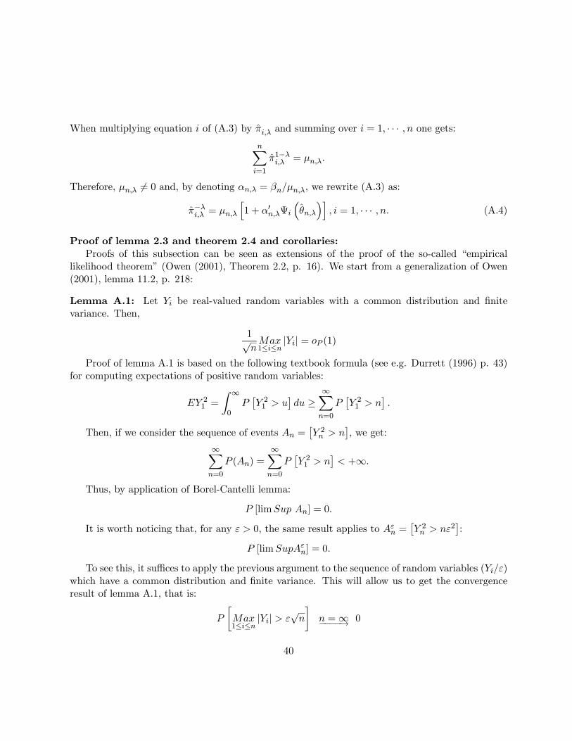
When multiplying equation i of (A.3) by πi,λ and summing over i = 1, · · · , n one gets:nXi=1

π1−λi,λ = µn,λ.

Therefore, µn,λ 6= 0 and, by denoting αn,λ = βn/µn,λ, we rewrite (A.3) as:

π−λi,λ = µn,λh1 + α0n,λΨi

³θn,λ

´i, i = 1, · · · , n. (A.4)

Proof of lemma 2.3 and theorem 2.4 and corollaries:Proofs of this subsection can be seen as extensions of the proof of the so-called “empirical

likelihood theorem” (Owen (2001), Theorem 2.2, p. 16). We start from a generalization of Owen(2001), lemma 11.2, p. 218:

Lemma A.1: Let Yi be real-valued random variables with a common distribution and finitevariance. Then,

1√nMax1≤i≤n

|Yi| = oP (1)

Proof of lemma A.1 is based on the following textbook formula (see e.g. Durrett (1996) p. 43)for computing expectations of positive random variables:

EY 21 =

Z ∞

0P£Y 21 > u

¤du ≥

∞Xn=0

P£Y 21 > n

¤.

Then, if we consider the sequence of events An =£Y 2n > n

¤, we get:

∞Xn=0

P (An) =∞Xn=0

P£Y 21 > n

¤< +∞.

Thus, by application of Borel-Cantelli lemma:

P [limSup An] = 0.

It is worth noticing that, for any ε > 0, the same result applies to Aεn =

£Y 2n > nε

2¤:

P [limSupAεn] = 0.

To see this, it suffices to apply the previous argument to the sequence of random variables (Yi/ε)which have a common distribution and finite variance. This will allow us to get the convergenceresult of lemma A.1, that is:

P

·Max1≤i≤n

|Yi| > ε√n

¸n =∞−−−−→ 0

40

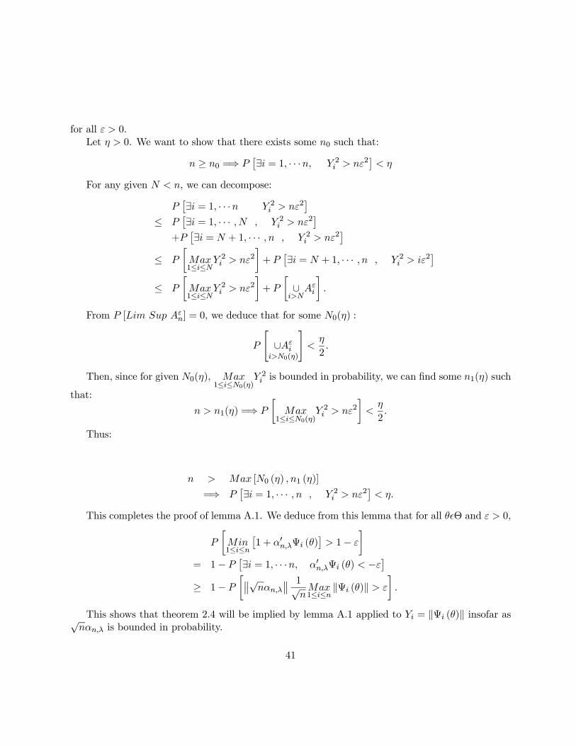
for all ε > 0.Let η > 0. We want to show that there exists some n0 such that:

n ≥ n0 =⇒ P£∃i = 1, · · ·n, Y 2i > nε

2¤< η

For any given N < n, we can decompose:

P£∃i = 1, · · ·n Y 2i > nε

2¤

≤ P£∃i = 1, · · · , N , Y 2i > nε

2¤

+P£∃i = N + 1, · · · , n , Y 2i > nε

2¤

≤ P

·Max1≤i≤N

Y 2i > nε2

¸+ P

£∃i = N + 1, · · · , n , Y 2i > iε2¤

≤ P

·Max1≤i≤N

Y 2i > nε2

¸+ P

·∪i>N

Aεi

¸.

From P [Lim Sup Aεn] = 0, we deduce that for some N0(η) :

P

"∪Aε

ii>N0(η)

#<

η

2.

Then, since for given N0(η), Max1≤i≤N0(η)

Y 2i is bounded in probability, we can find some n1(η) such

that:

n > n1(η) =⇒ P

·Max

1≤i≤N0(η)Y 2i > nε

2

¸<

η

2.

Thus:

n > Max [N0 (η) , n1 (η)]

=⇒ P£∃i = 1, · · · , n , Y 2i > nε

2¤< η.

This completes the proof of lemma A.1. We deduce from this lemma that for all θ²Θ and ε > 0,

P

·Min1≤i≤n

£1 + α0n,λΨi (θ)

¤> 1− ε

¸= 1− P £∃i = 1, · · ·n, α0n,λΨi (θ) < −ε

¤≥ 1− P

·°°√nαn,λ°° 1√nMax1≤i≤n

kΨi (θ)k > ε

¸.

This shows that theorem 2.4 will be implied by lemma A.1 applied to Yi = kΨi (θ)k insofar as√nαn,λ is bounded in probability.

41

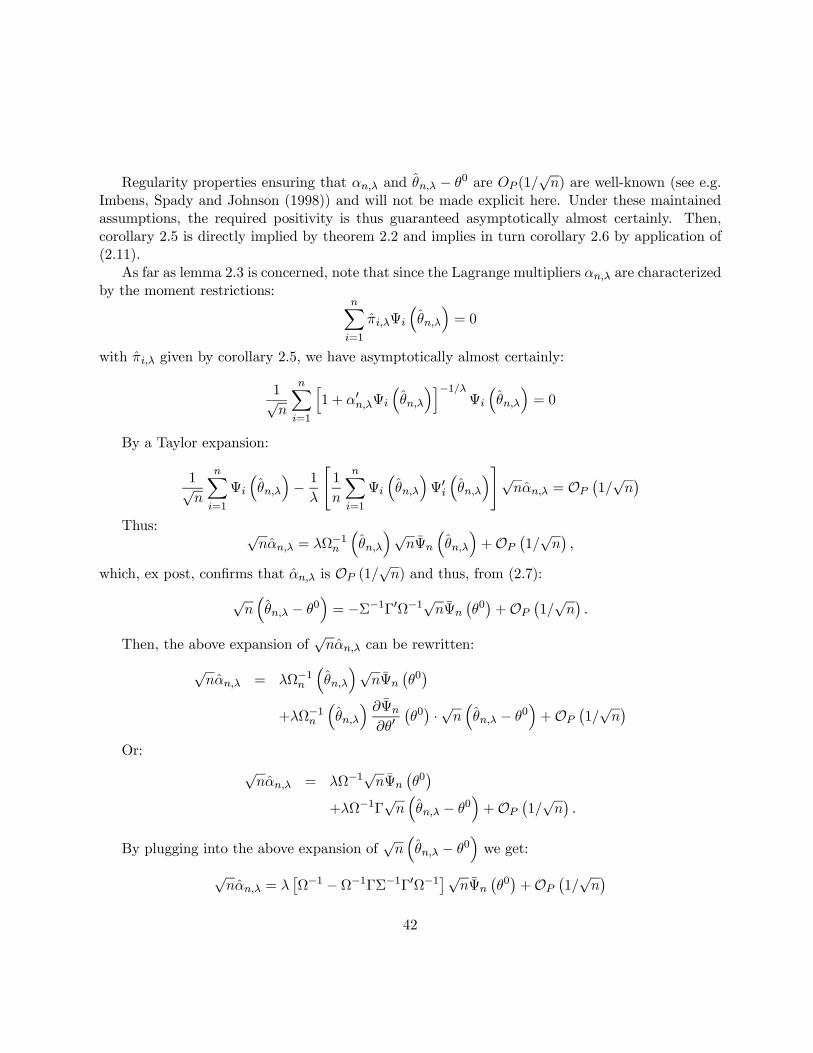
Regularity properties ensuring that αn,λ and θn,λ − θ0 are OP (1/√n) are well-known (see e.g.

Imbens, Spady and Johnson (1998)) and will not be made explicit here. Under these maintainedassumptions, the required positivity is thus guaranteed asymptotically almost certainly. Then,corollary 2.5 is directly implied by theorem 2.2 and implies in turn corollary 2.6 by application of(2.11).

As far as lemma 2.3 is concerned, note that since the Lagrange multipliers αn,λ are characterizedby the moment restrictions:

nXi=1

πi,λΨi

³θn,λ

´= 0

with πi,λ given by corollary 2.5, we have asymptotically almost certainly:

1√n

nXi=1

h1 + α0n,λΨi

³θn,λ

´i−1/λΨi

³θn,λ

´= 0

By a Taylor expansion:

1√n

nXi=1

Ψi

³θn,λ

´− 1

λ

"1

n

nXi=1

Ψi

³θn,λ

´Ψ0i³θn,λ

´#√nαn,λ = OP

¡1/√n¢

Thus: √nαn,λ = λΩ−1n

³θn,λ

´√nΨn

³θn,λ

´+OP

¡1/√n¢,

which, ex post, confirms that αn,λ is OP (1/√n) and thus, from (2.7):

√n³θn,λ − θ0

´= −Σ−1Γ0Ω−1√nΨn

¡θ0¢+OP

¡1/√n¢.

Then, the above expansion of√nαn,λ can be rewritten:

√nαn,λ = λΩ−1n

³θn,λ

´√nΨn

¡θ0¢

+λΩ−1n³θn,λ

´ ∂Ψn∂θ0

¡θ0¢ ·√n³θn,λ − θ0

´+OP

¡1/√n¢

Or:√nαn,λ = λΩ−1

√nΨn

¡θ0¢

+λΩ−1Γ√n³θn,λ − θ0

´+OP

¡1/√n¢.

By plugging into the above expansion of√n³θn,λ − θ0

´we get:

√nαn,λ = λ

£Ω−1 − Ω−1ΓΣ−1Γ0Ω−1¤√nΨn ¡θ0¢+OP ¡1/√n¢

42

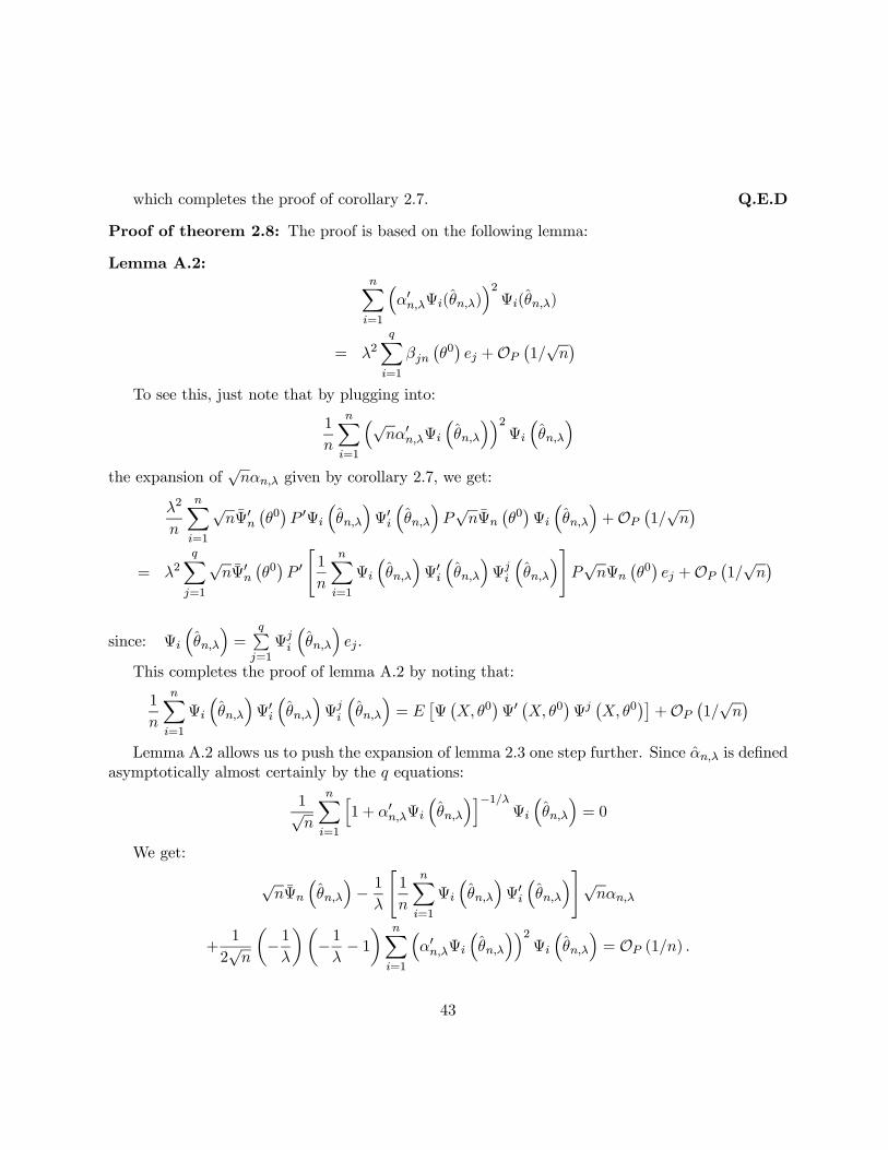
which completes the proof of corollary 2.7. Q.E.D

Proof of theorem 2.8: The proof is based on the following lemma:

Lemma A.2:nXi=1

³α0n,λΨi(θn,λ)

´2Ψi(θn,λ)

= λ2qXi=1

βjn¡θ0¢ej +OP

¡1/√n¢

To see this, just note that by plugging into:

1

n

nXi=1

³√nα0n,λΨi

³θn,λ

´´2Ψi

³θn,λ

´the expansion of

√nαn,λ given by corollary 2.7, we get:

λ2

n

nXi=1

√nΨ0n

¡θ0¢P 0Ψi

³θn,λ

´Ψ0i³θn,λ

´P√nΨn

¡θ0¢Ψi

³θn,λ

´+OP

¡1/√n¢

= λ2qXj=1

√nΨ0n

¡θ0¢P 0"1

n

nXi=1

Ψi

³θn,λ

´Ψ0i³θn,λ

´Ψji

³θn,λ

´#P√nΨn

¡θ0¢ej +OP

¡1/√n¢

since: Ψi

³θn,λ

´=

qPj=1Ψji

³θn,λ

´ej .

This completes the proof of lemma A.2 by noting that:

1

n

nXi=1

Ψi

³θn,λ

´Ψ0i³θn,λ

´Ψji

³θn,λ

´= E

£Ψ¡X, θ0

¢Ψ0¡X, θ0

¢Ψj¡X, θ0

¢¤+OP

¡1/√n¢

Lemma A.2 allows us to push the expansion of lemma 2.3 one step further. Since αn,λ is definedasymptotically almost certainly by the q equations:

1√n

nXi=1

h1 + α0n,λΨi

³θn,λ

´i−1/λΨi

³θn,λ

´= 0

We get:

√nΨn

³θn,λ

´− 1

λ

"1

n

nXi=1

Ψi

³θn,λ

´Ψ0i³θn,λ

´#√nαn,λ

+1

2√n

µ−1λ

¶µ−1λ− 1¶ nXi=1

³α0n,λΨi

³θn,λ

´´2Ψi

³θn,λ

´= OP (1/n) .

43

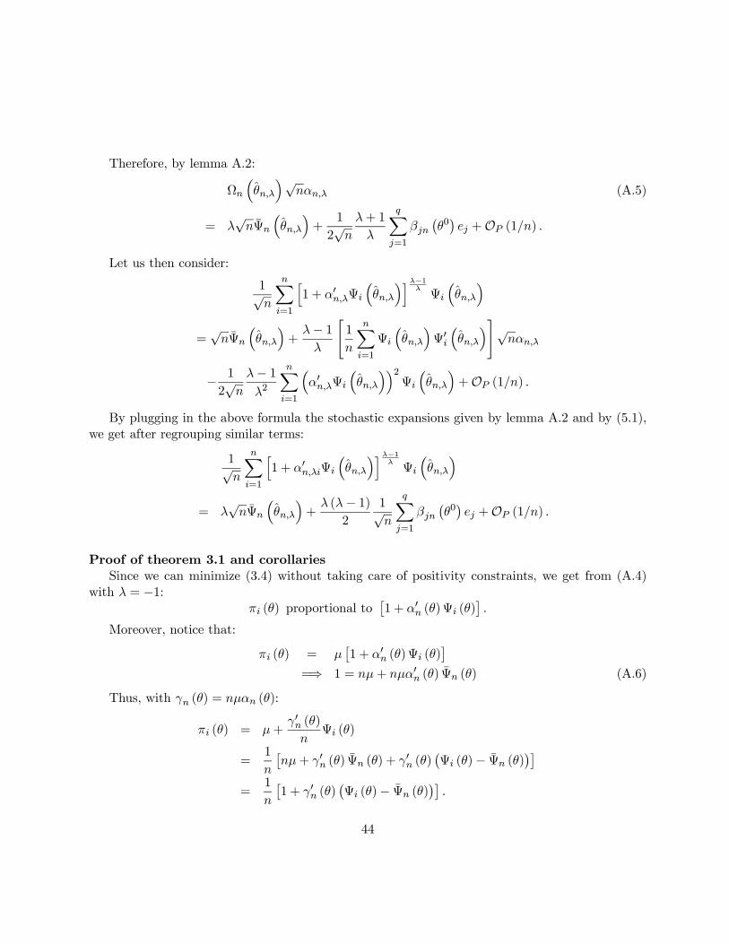
Therefore, by lemma A.2:

Ωn

³θn,λ

´√nαn,λ (A.5)

= λ√nΨn

³θn,λ

´+

1

2√n

λ+ 1

λ

qXj=1

βjn¡θ0¢ej +OP (1/n) .

Let us then consider:

1√n

nXi=1

h1 + α0n,λΨi

³θn,λ

´iλ−1λΨi

³θn,λ

´=√nΨn

³θn,λ

´+

λ− 1λ

"1

n

nXi=1

Ψi

³θn,λ

´Ψ0i³θn,λ

´#√nαn,λ

− 1

2√n

λ− 1λ2

nXi=1

³α0n,λΨi

³θn,λ

´´2Ψi

³θn,λ

´+OP (1/n) .

By plugging in the above formula the stochastic expansions given by lemma A.2 and by (5.1),we get after regrouping similar terms:

1√n

nXi=1

h1 + α0n,λiΨi

³θn,λ

´iλ−1λΨi

³θn,λ

´= λ

√nΨn

³θn,λ

´+

λ (λ− 1)2

1√n

qXj=1

βjn¡θ0¢ej +OP (1/n) .

Proof of theorem 3.1 and corollariesSince we can minimize (3.4) without taking care of positivity constraints, we get from (A.4)

with λ = −1:πi (θ) proportional to

£1 + α0n (θ)Ψi (θ)

¤.

Moreover, notice that:

πi (θ) = µ£1 + α0n (θ)Ψi (θ)

¤=⇒ 1 = nµ+ nµα0n (θ) Ψn (θ) (A.6)

Thus, with γn (θ) = nµαn (θ):

πi (θ) = µ+γ0n (θ)nΨi (θ)

=1

n

£nµ+ γ0n (θ) Ψn (θ) + γ0n (θ)


¢¤=

1

n

£1 + γ0n (θ)


¢¤.

44

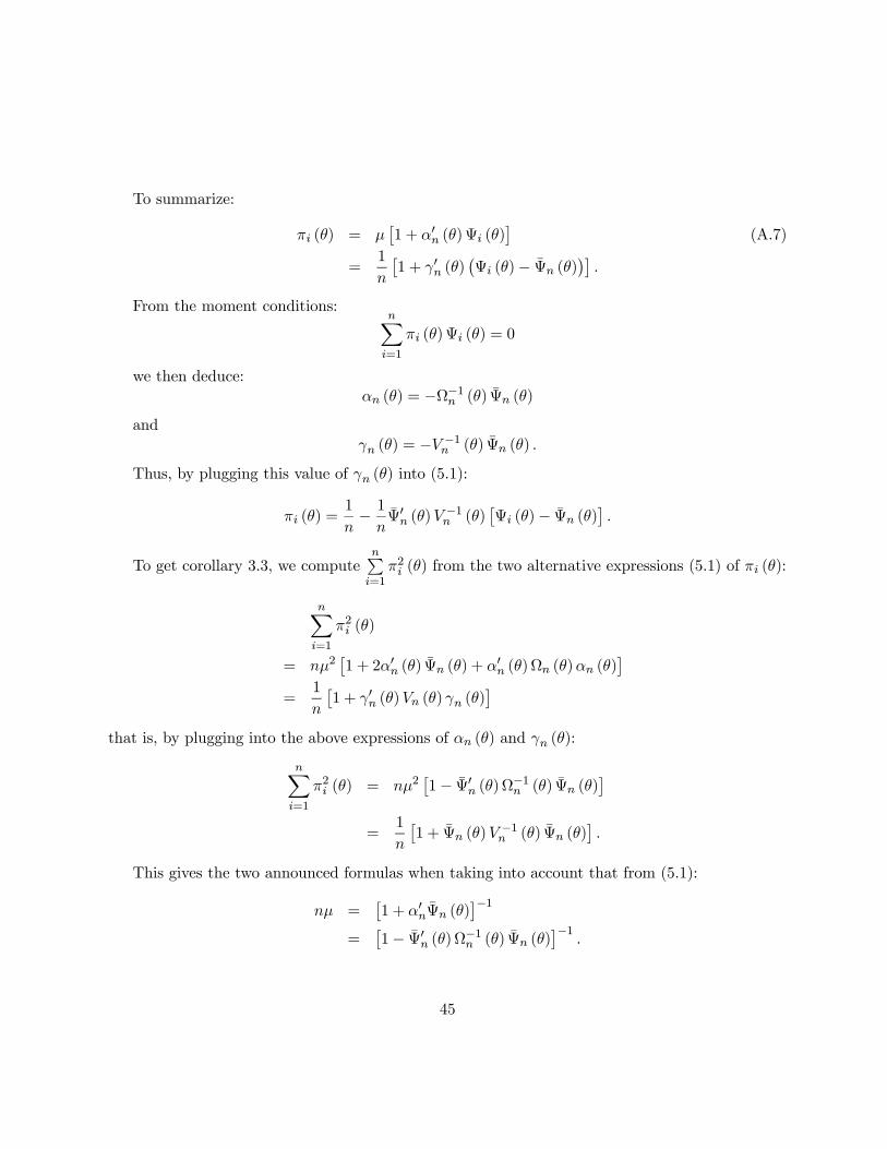
To summarize:

πi (θ) = µ£1 + α0n (θ)Ψi (θ)

¤(A.7)

=1

n

£1 + γ0n (θ)


¢¤.

From the moment conditions:nXi=1

πi (θ)Ψi (θ) = 0

we then deduce:αn (θ) = −Ω−1n (θ) Ψn (θ)

andγn (θ) = −V −1n (θ) Ψn (θ) .

Thus, by plugging this value of γn (θ) into (5.1):

πi (θ) =1

n− 1nΨ0n (θ)V

−1n (θ)


¤.

To get corollary 3.3, we computenPi=1

π2i (θ) from the two alternative expressions (5.1) of πi (θ):

nXi=1

π2i (θ)

= nµ2£1 + 2α0n (θ) Ψn (θ) + α0n (θ)Ωn (θ)αn (θ)

¤=

1

n

£1 + γ0n (θ)Vn (θ) γn (θ)

¤that is, by plugging into the above expressions of αn (θ) and γn (θ):

nXi=1

π2i (θ) = nµ2£1− Ψ0n (θ)Ω−1n (θ) Ψn (θ)

¤=

1

n

£1 + Ψn (θ)V

−1n (θ) Ψn (θ)

¤.

This gives the two announced formulas when taking into account that from (5.1):

nµ =£1 + α0nΨn (θ)

¤−1=

£1− Ψ0n (θ)Ω−1n (θ) Ψn (θ)

¤−1.

45

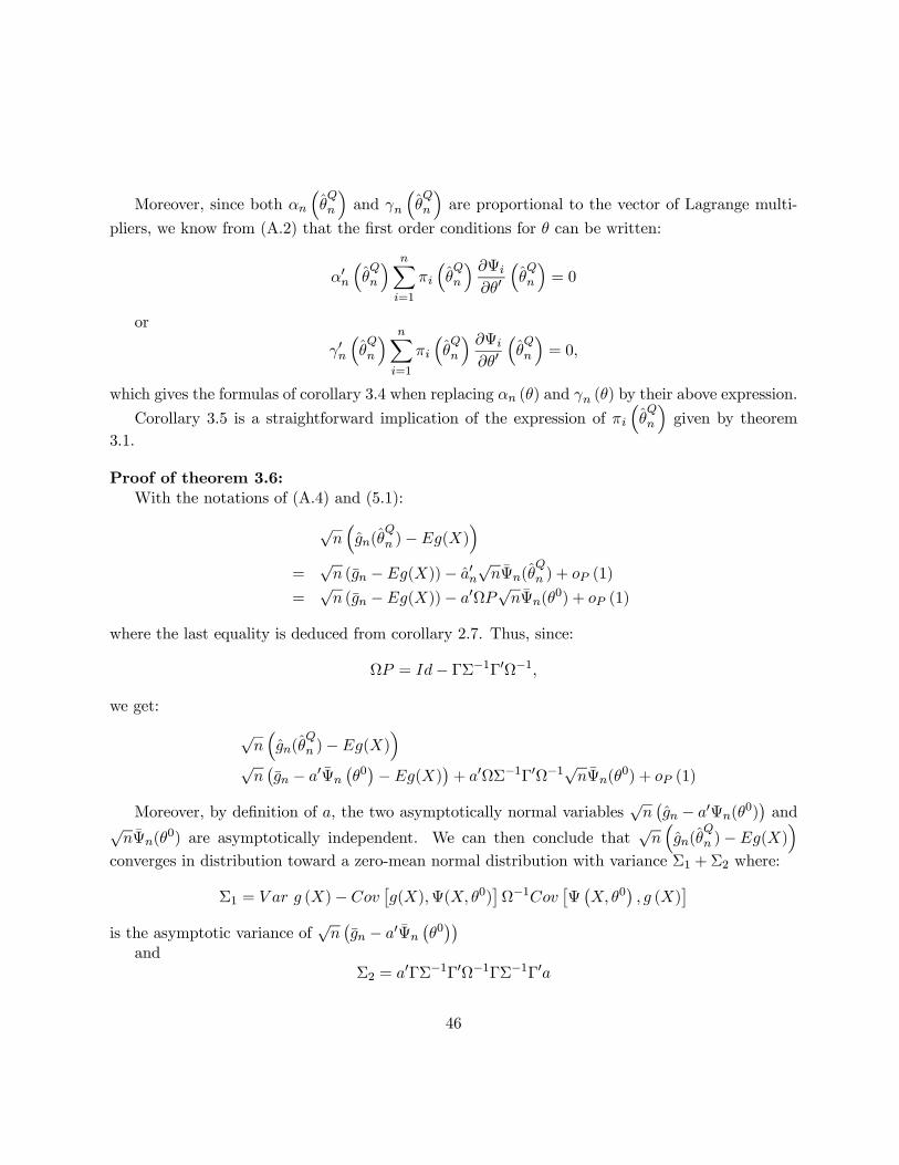
Moreover, since both αn

³θQn

ánd γn

³θQn

áre proportional to the vector of Lagrange multi-

pliers, we know from (A.2) that the first order conditions for θ can be written:

α0n³θQn

´ nXi=1

πi

³θQn

´ ∂Ψi∂θ0

³θQn

´= 0

or

γ0n³θQn

´ nXi=1

πi

³θQn

´ ∂Ψi∂θ0

³θQn

´= 0,

which gives the formulas of corollary 3.4 when replacing αn (θ) and γn (θ) by their above expression.

Corollary 3.5 is a straightforward implication of the expression of πi³θQn

´given by theorem

3.1.

Proof of theorem 3.6:With the notations of (A.4) and (5.1):

√n³gn(θ

Qn )−Eg(X)

´=√n (gn −Eg(X))− a0n

√nΨn(θ

Qn ) + oP (1)

=√n (gn −Eg(X))− a0ΩP

√nΨn(θ

0) + oP (1)

where the last equality is deduced from corollary 2.7. Thus, since:

ΩP = Id− ΓΣ−1Γ0Ω−1,

we get:

√n³gn(θ

Qn )−Eg(X)

´√n¡gn − a0Ψn

¡θ0¢−Eg(X)¢+ a0ΩΣ−1Γ0Ω−1√nΨn(θ0) + oP (1)

Moreover, by definition of a, the two asymptotically normal variables√n¡gn − a0Ψn(θ0)

¢and

√nΨn(θ

0) are asymptotically independent. We can then conclude that√n³gn(θ

Qn )−Eg(X)

ćonverges in distribution toward a zero-mean normal distribution with variance Σ1 +Σ2 where:

Σ1 = V ar g (X)− Cov£g(X),Ψ(X, θ0)

¤Ω−1Cov

£Ψ¡X, θ0

¢, g (X)

¤is the asymptotic variance of

√n¡gn − a0Ψn

¡θ0¢¢

andΣ2 = a

0ΓΣ−1Γ0Ω−1ΓΣ−1Γ0a

46

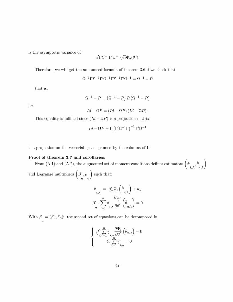
is the asymptotic variance ofa0ΓΣ−1Γ0Ω−1

√nΨn(θ

0).

Therefore, we will get the announced formula of theorem 3.6 if we check that:

Ω−1ΓΣ−1Γ0Ω−1ΓΣ−1Γ0Ω−1 = Ω−1 − P

that is:

Ω−1 − P = ¡Ω−1 − P¢Ω ¡Ω−1 − P¢or:

Id− ΩP = (Id− ΩP ) (Id− ΩP ) .This equality is fulfilled since (Id− ΩP ) is a projection matrix:

Id− ΩP = Γ ¡Γ0Ω−1Γ¢−1 Γ0Ω−1

is a projection on the vectorial space spanned by the columns of Γ.

Proof of theorem 3.7 and corollaries:

From (A.1) and (A.2), the augmented set of moment conditions defines estimatorsµπ˜ i,,λ

, θñ,λ

¶and Lagrange multipliers

µβñ

, µñ

¶such that:

π˜ i,λ

= β˜

0nΨi˜

µθñ,λ

¶+ µn

˜

β˜

0n

·nXi=1

π˜ i,λ

∂Ψi˜

∂θ0˜

µθñ,λ

¶= 0

With βñ

= (β0n, δn)0, the second set of equations can be decomposed in:β˜

0n

nPi=1

π˜ i,λ

∂Ψi∂θ0

³θn,λ

´= 0

δnnPi=1

π˜ i,λ

= 0

47

Therefore δn = 0 and the above first order conditions can be rewritten:π˜ i,λ

= β0nΨi³θn,λ

´+ µn

β0n ·nPi=1

π˜ i,λ

∂Ψi∂θ0

(θn,λ) = 0

They coincide with (A.1) and (A.2), and jointly with the corresponding constraints, define the

same estimators³πi,λ, θn,λ

ánd multipliers (βn, µn). Finally, ξn,λ is defined by the additional

constraintnXi=1

πi,λ

hg (Xi)− ξn,λ

i= 0

which completes the proof of theorem 3.7. Corollaries 3.8, 3.19 and 3.10 are obvious implications.Finally:

√nhg∗n(θ

Qn )− gn(θ

Qn )i

=εn(θ

Qn )

1 + εn(θQn )

√nhgn − gn(θQn )

i.

But, since all the πi(θQn ), i = 1, · · · , n are asymptotically nonnegative with probability 1:

εn(θQn ) = oP (1)

Since: √nhgn − gn(θQn )

i= OP (1)

We can conclude that: √nhg∗n(θ

Qn )− gn(θ

Qn )i= oP (1) .

Proof of theorem 3.12:We want to compare the two estimators θn and θn,1 defined respectively by:

gn

³θn

´= 0 and fn

³θn,1

´= 0

where:

fn (θ) =

·En,1

∂Ψ0i∂θ

(θ)

¸ hVn,1Ψi (θ)

i−1Ψn (θ)

andgn (θ) =

hΓQ0n

³θn

í hΩQ0n

³θn

í−1Ψn (θ) +OP (1/n

√n).

48

In order to apply Robinson (1988), theorem 1, we need to check that the two properties of hisassumption (A.2) are fulfilled. A first condition is:

∂gn∂θ0

¡θ0¢= G+ oP (1)

with G nonsingular matrix. This condition is fulfilled here with:

G = 2Γ0¡θ0¢ £Ω¡θ0¢¤−1

Γ¡θ0¢.

A second condition is akin to a kind of asymptotic continuity of∂gn∂θ0

(θ) at the point θ0. This

assumption will be maintained here.Then, we can conclude from Robinson (1988) that:

θn − θn,1 = OP³°°°gn ³θn,1´°°°´

= OP³°°°gn ³θn,1´− fn ³θn,1´°°°´ .

Since√nΨn

³θn,1

´= OP (1), we will then get the announced result if we show that:°°°°ΓQn ³θn´− En,1∂Ψi∂θ0

³θn,1

´°°°° = OP (1/n)and °°°ΩQn ³θn´− Vn,1Ψi ³θn,1´°°° = OP (1/n) .

Since θn − θQn = OP (1/n), a simple Taylor expansion argument actually gives:°°°ΓQn ³θn´− ΓQn (θQn )°°° = OP (1/n)

and °°°ΩQn ³θn´− ΩQn (θQn )°°° = OP (1/n) .Therefore, by a triangle inequality argument, we conclude that we just need to show that:°°°°ΓQn (θQn )− En,1∂Ψi∂θ0

(θn,1)

°°°° = OP (1/n)and °°°ΩQn ³θQn ´− Vn,1Ψi ³θn,1´°°° = OP (1/n) .

This is a straightforward consequence of corollary 3.8.

49

Proof of Theorem 4.1:When optimizing (4.6) under the constraints (4.8), the Lagrangian can be written:

` =nXi=1

nXj=1

wλijh

(λ) (πi,j)

−nXi=1

β0inXj=1

πijΨj (θ)

−nXi=1

µi

nXj=1

πij − 1 .

Then, the estimators πi,j,λ, θn,λ are characterized, for well-suited values βin and µin of theLagrange multipliers, by the following first order conditions:

wλijπ

−λi,j,λ = β0inΨj

³θn,λ

´+ µin, i, j = 1, · · · , n, (A.8)

nXi=1

β0innXj=1

πi,j,λ∂Ψj∂θ0

³θn,λ

´= 0 (A.9)

When multiplying equation (i, j) of (A.8) by πi,j,λΨ0j

³θn,λ

´and summing over j = 1, · · · , n

one gets, for i = 1, · · · , n:nXj=1

wλijπ

1−λi,j,λΨ

0j

³θn,λ

´= β0in

nXj=1

πi,j,λΨj

³θn,λ

´Ψ0j³θn,λ

´,

since, by definition:nXj=1

πi,j,λΨ0j

³θn,λ

´= 0.

Therefore, the q-vector of Lagrange multipliers associated to the conditional moment restrictionsgiven Z = Zi is:

βin =

nXj=1

πi,j,λΨj

³θn,λ

´Ψ0j³θn,λ

´−1 nXj=1

wλijπ

1−λi,j,λΨj

³θn,λ

´.

By virtue of (A.9), this gives the announced result.

Proof of theorem 4.2:

50

From (A.8), we have:

π−λi,j,λ = w−λi,j

hµin + β0inΨj

³θn,λ

´i(A.10)

when multiplying equation (i, j) of (A.10) by wλi,jπi,j,λ and summing over j = 1, · · · , n, one gets:

nXj=1

wλi,jπ

1−λi,j,λ = µi,n.

Therefore, µi,n 6= 0 and, by denoting µi,n = µi,n,λ and αi,n,λ = βi,n/µi,n, we rewrite (A.10) as:

π−λi,j,λ = µi,n,λw−λi,j

h1 + α0i,n,λΨj

³θn,λ

´i. (A.11)

Proof of theorem 4.3 and corollaries:Since we can minimize (4.19) without taking care of positivity constraints, we get from theorem

4.2 with λ = −1: For i = 1, · · · , n the πi,j(θ), j = 1, · · · , n, are proportional to:

wij£1 + α0i,n(θ)Ψj(θ)

¤.

Moreover, notice that:

πi,j(θ) = µiwij£1 + α0i,n(θ)Ψj(θ)

¤=⇒ 1 = µi + µiα

0i,n(θ)Ψj(θ). (A.12)

Thus, with γi,n(θ) = µiαi,n(θ):

πi,j(θ) = µiwij + wijγ0i,n(θ)Ψi(θ) + wijγ

0i,n(θ)

£Ψj(θ)− Ψi(θ)

¤wij +wijγ

0i,n(θ)

£Ψj(θ)− Ψi(θ)

¤.

From the moment conditionsnXj=1

πi,j(θ)Ψj(θ) = 0

We then deduce:

αi,n(θ) = −Ω−1n (θ |Zi )Ψi(θ)and

γi,n(θ) = −V −1n (θ |Zi )Ψi(θ).

Thus, by plugging this value of γi,n(θ) into the above expression of πi,j(θ) we get:

πi,j(θ) = wij − wijΨ0j(θ)V −1n (θ |Zi )£Ψj(θ)− Ψi(θ)

¤.

51

To get corollary 4.4, we computenPi=1

nPj=1

π2i,j(θ)

wijfrom the two alternative expressions of πi,j(θ):

Xi,j

π2i,j(θ)

wij=

nXi=1

µ2i

nXj=1

wij£1− Ψ0i(θ)Ω−1n (θ |Zi )Ψj(θ)

¤2=

nXi=1

nXj=1

wij£1− Ψ0i(θ)V −1n (θ |Zi )

¡Ψj(θ)− Ψi(θ)

¢¤2.

Therefore: Xi,j

π2i,j(θ)

wij=

nXi=1

µ2i£1− Ψ0i(θ)Ω−1n (θ |Zi )Ψj(θ)

¤=

nXi=1

£1 + Ψ0i(θ)V

−1n (θ |Zi )Ψi(θ)

¤.

Since by (A.12):

µi =£1 + α0i,n(θ)Ψi(θ)

¤−1=£1− Ψ0i(θ)Ω−1n (θ |Zi )Ψj(θ)

¤−1we conclude that:

nXi=1

µ2i£1− Ψ0i(θ)Ω−1n (θ |Zi )Ψi(θ)

¤=

nXi=1

£1− Ψ0i(θ)Ω−1n (θ |Zi )Ψi(θ)

¤−1

By comparing (A.8) and (A.12), we see that βin = γin, so that plugging the value of γin in firstorder conditions (A.9) provides the characterization of corollary 4.5.

52

References

[1] Ai., C. and Chen, X. (2003), “Efficient Estimation of Models with Conditional Moment Re-strictions Containing Unknown Functions”, Econometrica 71, 6, 1795-1843.

[2] Ai, C. and Chen, X. (2001), “Efficient Sieve Minimum Distance Estimation of SemiparametricConditional Moment Models”, W.P.

[3] Altonji, J. G. and Segal, L. M. (1996), “Small Sample Bias in GMM Estimation of CovarianceStructures”, Journal of Economic and Business Statistics 14, 353-366.

[4] Andrews, D. W. K. (1999), “Moment Selection Procedures for Generalized Method of MomentsEstimation”, Econometrica 67, 543-564.

[5] Back, K. and Brown, D. P. (1993) “Implied probabilities in GMM estimators”, Econometrica61, No.4, 971-975.

[6] Baggerly, K. A. (1998) “Empirical Likelihood as a goodness-of-fit Measure”, Biometrika 85,No.3, 535-547.

[7] Bera, A. K. and Bilias Y. (2002), “The MM, ME, ML, EL, EF and GMM approaches toestimation: a synthesis”, Journal of Econometrics 107, 51-86.

[8] Bonnal, H. (2003), “Estimation d’une distribution de probabilité sous contraintes de moments”,forthcoming, Ph.D. thesis, Université de Rennes 1.

[9] Chamberlain, G. (1987) “Asymptotic Efficiency in Estimation with Conditional Moment Re-strictions”, Journal of Econometrics 34, 305-334.

[10] Corcoran, S. (1998), “Bartlett Adjustment of Empirical Discrepancy Statistics”, Biometrika85, No.4, 967-972.

[11] Donald, S. G., Imbens, G. W. and Newey, W.K. (2001), “Empirical Likelihood Estimation andConsistent Tests with Conditional Moment Restrictions”, W.P.

[12] Donald, S. G. and Newey, W.K. (2000), “A Jackknife Interpretation of the Continuous Up-dating Estimator”, Economics Letters 67, 239-243.

[13] Durrett, R. (1996), “Probability: Theory and Examples, Second Edition”, Duxbury Press,ITP.

[14] Fieller, F.C. and H.O. Hartley (1954), “Sampling with Control Variables”, Biometrika 41,3/4, 494-501.

53

[15] Godambe, V. P. and Thompson (1989), “An Extension of Quasi-likelihood Estimation” (withdiscussion), Journal of Statistical Planning and Inference 22, 137-172.

[16] Hall, A. (2000), “Covariance Matrix Estimation and the Power of the Overidentifying Restric-tions Test”, Econometrica 68, 1517-1527.

[17] Hansen, L. P. (1982), “Large Sample Properties of Generalized Method of Moments Estima-tors”, 1982, Econometrica 50, No.4, 1029-1054.

[18] Hansen, L. P., Heaton, J. and Yaron, A. (1996), “Finite-Sample Properties of Some AlternativeGMM Estimators”, Journal of Business & Economic Statistics 14, No.3, 262-280.

[19] Imbens, G. W. (1997), “One-Step Estimators for Over-identified Generalized Method of Mo-ments Models”, Review of Economic Studies 64, No.1, 359-383.

[20] Imbens, G. W., Spady, R. H. and Johnson P. (1998), “Information Theoretic Approaches toInference in Moment Conditions Models”, Econometrica 66, No.2, 333-357.

[21] Kitamura, Y. and Stutzer, M. (1997),. “An Information Theoretic Alternative to GeneralizedMethod of Moments Estimation”, Econometrica 65, No.4, 861-874.

[22] Kitamura, Y. Tripathi, G. and Ahn, H. (2000), “Empirical Likelihood-based Inference in Con-ditional Moment Restriction Models”, W.P.

[23] Ledoit, O. and M. Wolf (2001), “Improved Estimation of the Covariance Matrix of Stock Re-turns with an Application to Portfolio Selection”, Journal of Empirical Finance, forthcoming.

[24] Maasoumi E. (1993), “A Compendium to Information Theory in Economics and Economet-rics”, Econometric Reviews, 12(2), 137-181.

[25] Newey, W. K. (1993), “Efficient Estimation of Models with Conditional Moment Restrictions”in G. S. Maddala, C. R. Rao and H. D. Vinod Eds, Handbook of Statistics, volume 11: Econo-metrics, North Holland.

[26] Newey, W. and R. J. Smith (2004), “Higher Order Properties of GMM and Generalized Em-pirical Likelihood Estimators”, Econometrica 72, 1, 219-255.

[27] Owen, A. (1990) “Empirical Likelihood Ratio Confidence Regions”, The Annals of Statistics18, No.1, 90-120.

[28] Owen, A. (1991) “Empirical Likelihood for Linear Models”, The Annals of Statistics 19, No.4,1725-1747.

[29] Owen, A. (2001) Empirical Likelihood, Chapman & Hall.

54

[30] Pakes, A. and Pollard, D. (1989), “Simulation and the Asymptotics of Optimization Estima-tors”, Econometrica 57, No. 5, 1027-1057.

[31] Qin, J. and Lawless, J. (1994), “Empirical Likelihood and General Estimating Equations”,The Annals of Statistics 22, No.1, 300-325.

[32] Read, T. R., C. and Cressie, N. (1988) Goodness-of-Fit Statistics for Discrete MultivariateData, 1988, Springer-Verlag, New York.

[33] Robinson, P. M. (1988), “The Stochastic Difference Between Econometric Statistics”, Econo-metrica, 56, 531-548.

[34] Rothenberg, T. J. (1984), “Approximating the Distributions of Econometric Estimators andTest Statistics”, in Handbook of Econometrics, Vol. 2, ed. by Z. Griliches and M. D. Intriligator,North-Holland.

[35] Severini, T.A. and G. Tripathi (2001), “A Simplified Approach to Computing EfficiencyBounds in Semiparametric Models”, Journal of Econometrics 102, 23-66.

[36] Smith, R. J. (2000), Empirical Likelihood Estimation and Inference, in “Applications of Dif-ferential Geometry to Econometrics”, P. Marriott and M. Salmon Eds, Cambridge, UniversityPress.

[37] Zellner, A. (1991), “Bayesian Methods and Entropy in Economics and Econometrics,” inGrandy, W. T. and Schick, L. H. (eds.)., Maximum Entropy and Bayesian Methods, Dor-drecht/Boston/London: Kluwer Academic Publishers, 17-31.

[38] Zellner, A. (2003), “Some Aspects of the History of Bayesian Information Processing”, W.P.Chicago GSB.

[39] Zellner, A. and Tobias, J. (2001), “Further Results on Bayesian Method of Moments Analysisof the Multiple Regression Model”, International Economic Review 42, No. 1, 121-140.

55

2004s-18 On the Efficient Use of the Informational Content of...

Documents

Transcript of 2004s-18 On the Efficient Use of the Informational Content of...