© 2004 by Ya Meng. All rights reservedccc.illinois.edu/s/Theses/2004_MENG_Ya_PhDThesis.pdf · IN...

MODELING INTERFACIAL SLAG LAYER PHENOMENA IN THE SHELL/MOLD GAP IN CONTINUOUS CASTING OF STEEL

BY

YA MENG

B.S., Central South University of Technology, 1995 M.E.N.G.R., Central South University of Technology, 1998

DISSERTATION

Submitted in partial fulfillment of the requirements for the degree of Doctor of Philosophy in Materials Science and Engineering

in the Graduate College of the University of Illinois at Urbana-Champaign, 2004

Urbana, Illinois

iii

ABSTRACT

Heat transfer and lubrication of interfacial gap between the mold and the

solidifying steel shell control the final product quality of continuous casting of steel.

Previous solidification and heat transfer models for continuous casting of steel are

evaluated, focusing on the treatment of the interfacial gap. Experimental work on mold

slag properties and their effect on heat transfer and lubrication are reviewed.

A new lubrication and friction model of slag in the interfacial gap was combined

into an existing 1-D heat transfer model, CON1D. Analytical transient models of liquid

slag flow and solid slag stress have been coupled with a finite-difference model of heat

transfer in the mold, gap and steel shell to predict transient shear stress, friction, slip and

fracture of the slag layers. The consistency and accuracy of the model is validated by

comparing with analytical solutions and with results from commercial codes.

Experimental work is conducted to measure the properties of slag powder,

including the friction coefficient at different temperatures and viscosity at lower

temperature than previously measured. DSC, dip thermocouple and atomization tests are

conducted to construct CCT curves and to predict critical cooling rates of two slag

powders, which have different crystallization tendencies. XRD, Polarized Transmission

Light Microscopy and SEM are used to analyze the composition of the mold powder and

re-solidified slag samples and to determine the crystalline/glassy microstructure.

The CON1D model predicts shell thickness, temperature distributions in the mold

and shell, thickness of the re-solidified and liquid powder layers, heat flux profiles down

the wide and narrow faces, mold water temperature rise, ideal taper of the mold walls,

iv

and other related phenomena. Plants measurements from operating casters were collected

to calibrate the model.

The model is then applied to study the effect of casting speed and mold powder

viscosity properties on slag layer behavior between the oscillating mold wall and the

solidifying steel shell. The study finds that liquid slag lubrication would produce

negligible stresses. Lower mold slag consumption rate leads to higher solid friction and

results in solid slag layer fracture and movement if it falls below a critical value.

Crystalline slag tends to fracture near the meniscus and glassy slag tends to fracture near

mold exit. Mold friction and fracture are governed by lubrication consumption rate,

which is total consumption rate subtracting the slag consumption in the oscillation marks.

Medium casting speed may be the safest to avoid slag fracture due to its having the

lowest critical lubrication consumption rate. The high measured friction force in

operating casters could be due to three sources: an intermittent moving solid slag layer,

excessive mold taper or mold misalignment.

The model is also applied to interpret the crystallization behavior of slag layers in

the interfacial gap between the mold and the steel shell. A mechanism for the formation

of this crystalline layer is proposed that combines the effects of a shift in the viscosity

curve, a decrease in the liquid slag conductivity due to partial crystallization, and an

increase in the solid slag layer roughness corresponding to a decrease in solid layer

surface temperature with distance down the mold. When the shear stress exceeds the slag

shear strength before the axial stress accumulates to the fracture strength, the slag could

shear longitudinally inside the layers.

v

To my family

vi

ACKNOWLEDGEMENTS

I would like to express my sincere gratitude to my advisor, Professor Brian G.

Thomas for his guidance, support and encouragement through out of this work. I feel

fortunate for having opportunity to learning a great deal from him both academically and

personally. Also thanks to my committee members, Prof. Jonathan Dantzig, Prof. Ian

Robertson, Prof. Pascal Bellon, Prof. David Payne and Prof. Waltraud Kriven, who

offered guidance and support.

I would like to thank members of the Continuous Casting Consortium at UIUC,

including Accumold (Huron Park, Ontario, Canada), AK Steel (Middletown, OH),

Allegheny Ludlum Corporation (Brackenridge, PA ), Armco Inc. (Middletown, OH),

Bethlehem Steel (Richfield, OH), BHP Steel (Australia ), Columbus Stainless Pty Ltd.

(Mpumulanga, South Africa), Hatch Associate Consultants (Buffalo, NY), Inland Steel

Company (East Chicago, IN), LTV Steel Company (Richfield OH), Postech (Pohang,

Kyoungbuk, Korea), and Stollberg (Niagara Falls, NY) for their continued support of my

research.

Thanks to Dr. Ron J. O’Malley at Nucor Steel and Darrell Sturgill at Stollberg for

their measurements and suggestions. Prof. Hani Henein and Arvind Prasad at University

of Alberta, Canada help with CCT tests; Dr Xiaoqiang Hou at The Center for Cement

Composite Materials, UIUC with DSC tests, Prof. Andreas Polycarpou and Tim Solzak at

Mechanic Engineering Department with friction tests and Prof. Craig Lundstrom and

Fang Huang at Geology Department with polarized microscopy, Mr. John Bukowski, Mr.

Scott Robunson for help on analysis methods. Some analyses are carried out in the Center

vii

for Microanalysis of Materials, University of Illinois, which is partially supported by the

U.S. Department of Energy under grant DEFG02-91-ER45439.

I am greatly indebted to all members of Metals Processing Simulation research

group, Dr. Chunsheng Li, Dr. Hua Bai, Dr. Lifeng Zhang, Dr. Young-Mok Won, Dr.

Joydeep Sengupta, Lan Yu, Tiebiao Shi, Quan Yuan, Bin Zhao and Claudio Ojeda, I

could not imagine being able to complete my research without their unselfish help, advice

and encouragement.

Finally, I am thankful to all of my friends and my whole family: my parents,

sister, my husband and my baby who endured this long process with me, always offering

support and love.

viii

TABLE OF CONTENTS

page

LIST OF TABLES............................................................................................................ xii

LIST OF FIGURES .........................................................................................................xiii

NOMENCLATURE ....................................................................................................... xvii

CHAPTER 1. INTRODUCTION ....................................................................................... 1

1.1 Background ......................................................................................................... 1

1.2 Process Overview................................................................................................ 1

1.3 Mold Slag ............................................................................................................ 4

1.4 Objectives............................................................................................................ 6

1.5 Methodology ....................................................................................................... 7

1.6 Figures................................................................................................................. 9

CHAPTER 2. LITERATURE REVIEW .......................................................................... 10

2.1 Mathematical Modeling .................................................................................... 10

2.1.1 Steel Solidification Models ..................................................................... 10

2.1.2 Mold Heat Transfer and Distortion Model.............................................. 11

2.1.3 Interfacial Model..................................................................................... 13

2.2 Plants Measurements......................................................................................... 16

2.2.1 Thermal Response................................................................................... 16

2.2.2 Friction Signal......................................................................................... 17

2.3 Mold Powder Properties.................................................................................... 18

2.3.1 Mold Powder Composition ..................................................................... 18

2.3.2 Viscosity.................................................................................................. 20

2.3.3 Solidification Temperature...................................................................... 22

2.3.4 Crystallization Behavior ......................................................................... 23

2.3.5 Thermal Conductivity ............................................................................. 25

2.3.6 Slag Selection Criteria ............................................................................ 25

2.4 Tables and Figures ............................................................................................ 26

ix

CHAPTER 3. MODEL DESCRIPTION AND VALIDATION....................................... 33

3.1 Steel Solidification Model................................................................................. 33

3.1.1 Superheat Delivery.................................................................................. 33

3.1.2 Heat Conduction in the Solidifying Steel Shell ...................................... 34

3.1.3 Microsegregation Model ......................................................................... 35

3.1.4 Ideal Taper .............................................................................................. 36

3.1.5 Steel Properties ....................................................................................... 37

3.1.6 Steel Solidification Model Validation..................................................... 40

3.2 Heat Transfer and Mass Balance in Slag........................................................... 40

3.2.1 Heat transfer Across the Interfacial Gap................................................. 40

3.2.2 Mass and Momentum Balance on Powder Slag Layers.......................... 43

3.3 Lubrication and Friction Model in Gap............................................................. 46

3.3.1 Liquid Slag Layer Flow Model ............................................................... 46

3.3.2 Liquid Slag Layer Flow Model Validation ............................................. 49

3.3.3 Solid Slag Layer Stress Model................................................................ 50

3.3.4 Solid Slag Layer Stress Model Validation .............................................. 52

3.3.5 Solid Slag Layer Fracture Model ............................................................ 53

3.3.6 Mold Friction .......................................................................................... 54

3.4 Mold Heat Transfer Model................................................................................ 55

3.4.1 Heat Conduction in the Mold.................................................................. 55

3.4.2 Convection to the Cooling Water............................................................ 56

3.5 Spray Zones....................................................................................................... 58

3.6 Solution Methodology....................................................................................... 59


CHAPTER 4. SLAG PROPERTY MEASUREMENTS & CHARACTERIZATION .... 77

4.1 Chemical Composition...................................................................................... 77

4.2 Friction Coefficient ........................................................................................... 78

4.2.1 Sample Preparation and Instrumentation ................................................ 78

4.2.2 Experimental Procedure .......................................................................... 79

4.2.3 Results and Discussion............................................................................ 80

4.3 Viscosity............................................................................................................ 82

x

4.4 Crystallization Study ......................................................................................... 83

4.4.1 Experimental Methods ............................................................................ 84

4.4.2 X-ray Diffraction (XRD)......................................................................... 87

4.4.3 Results and Discussion............................................................................ 87

4.5 Slag Film Microscopy ....................................................................................... 92

4.5.1 Polarized Transmitted Light Microscopy................................................ 92

4.5.2 Scanning Electron Microscopy (SEM) ................................................... 94


CHAPTER 5. MODEL CALIBRATION....................................................................... 111

5.1 Mold Cooling Water Temperature Rise .......................................................... 112

5.2 Mold Temperatures ......................................................................................... 113

5.3 Shell Thickness ............................................................................................... 114

5.4 Powder Layer Thickness ................................................................................. 116

5.5 Shell Surface Temperature .............................................................................. 117

5.6 Tables and Figures .......................................................................................... 119

CHAPTER 6. MODEL APPLICATIONS...................................................................... 124

6.1 Typical Results ................................................................................................ 125

6.2 Crystallization Behavior.................................................................................. 126

6.3 Critical Slag Consumption Rate...................................................................... 127

6.4 Mold Friction................................................................................................... 128

6.4.1 Attached Solid Slag Layer .................................................................... 128

6.4.2 Moving Solid Slag Layer ...................................................................... 129

6.4.3 Friction Variation during an Oscillation Cycle..................................... 130

6.4.4 Total Mold Friction Force..................................................................... 131

6.5 Other Applications .......................................................................................... 132

6.5.1 Boiling Prediction ................................................................................. 132

6.5.2 Breakout Analysis ................................................................................. 133

6.5.3 Crack Formation Analysis .................................................................... 133


CHAPTER 7. SLAG CONSUMPTION AND CASTING SPEED STUDY ................. 142

7.1 Effect of Casting Speed on Heat Transfer and Shell Growth.......................... 142

xi

7.2 Effect of Slag Properties on Critical Consumption Rate................................. 144

7.3 Effect of Casting Speed on Critical Consumption Rate .................................. 145

7.4 Effect of Casting Speed on Friction Stress...................................................... 147


CHAPTER 8. CASE STUDY: INTERFACIAL GAP ANALYSIS FOR AK STEEL

CASTER............................................................................................... 156

8.1 Input Conditions.............................................................................................. 156

8.2 Heat Transfer Results ...................................................................................... 158

8.3 Crystallization Behavior.................................................................................. 160

8.4 Friction Results ............................................................................................... 163


CHAPTER 9. CONCLUSIONS ..................................................................................... 170

APPENDIX A. FDM SOLUTION OF STEEL SOLIDIFICATION MODEL .............. 174

APPENDIX B. CARBON STEEL THERMAL PROPERTIES FUNCTIONS ............. 177

APPENDIX C. HEAT LOSS FROM MOLD SLAG SOLIDIFICATION AND

COOLING ............................................................................................ 179

APPENDIX D. ANALYTICAL SOLUTION FOR 2-D HEAT CONDUCTION IN

THE MOLD.......................................................................................... 180

APPENDIX E. MOLD THICKNESS............................................................................. 182

APPENDIX F. WATER PROPERTIES IN MOLD COOLING CHANNEL................ 183

APPENDIX G. MANUFACTURER REPORTED SLAG COMPOSITION ................ 184

APPENDIX H. AK STEEL BREAKOUT SHELL GROWTH ..................................... 185

APPENDIX I. CON1D VERSION 7.5 SAMPLE INPUT AND OUTPUT FILES ....... 186

REFERENCES .............................................................................................................. 195

VITA .............................................................................................................. 212

xii

LIST OF TABLES

page

Table 2.1 Typical Chemistry Range for Mold Slag .................................................. 26

Table 2.2 Effect of Components on Viscosity and Crystallization Temperature of

Mold Slags ................................................................................................ 26

Table 3.1 Equilibrium Partition Coefficient, Diffusion Coefficient, and Liquidus

Line Slopes of the Solute Elements .......................................................... 61

Table 3.2 Constants Used in Analytical Solution and Validation Case for Steel

Solidification Model ................................................................................. 62

Table 3.3 Typical Casting Condition and Simulation Parameters for Transient

Interfacial Gap Model ............................................................................... 63

Table 3.4 Simulation Parameters in Liquid Slag Layer Model Validation Cases .... 64

Table 3.5 Terms in Eq.(3.26) for Case (b) at t=0.18s, x=0.16mm (unit: N/m3) ....... 64

Table 4.1 Mold Powder Composition (wt%) ............................................................ 95

Table 4.2 HTT Friction Tests.................................................................................... 96

Table 4.3 Dip Thermocouple Tests Cooling Rates Range (oC/sec).......................... 96

Table 4.4 Slag Annealing Treatment ........................................................................ 96

Table 4.5 Phases Present in Slag S1 from Dip TC and Devitrification Tests........... 97

Table 4.6 Phases Present in Slag S2 from Dip TC and Devitrification Tests........... 97

Table 5.1 Standard Input Conditions for Model Calibration .................................. 119

Table 5.2 Input Conditions for Sub-Mold Calibration (China Steel Case)............. 120

Table 5.3 Input Spray Zone Variables (China Steel Case) ..................................... 120

Table 6.1 Slag Composition and Properties............................................................ 134

Table 6.2 Case Study Parameters............................................................................ 134

Table 7.1 Parametric Study Conditions for Effect of Casting Speed...................... 148

Table 7.2 Mold Oscillation Practice with Casting Speed ....................................... 148

Table 8.1 Input Conditions for AK Steel Case ....................................................... 164

Table G.1 Mold Powder Composition Reported by Suppliers (wt%) ..................... 184

Table H.1 AK Steel Breakout Shell Drainage Time vs. Distance ........................... 185

xiii

LIST OF FIGURES

page

Figure 1.1 Steel continuous casting process................................................................. 9

Figure 1.2 Schematic of CC phenomena showing slag layers ..................................... 9

Figure 2.1 Variation of mold hot face temperature and heat flux .............................. 27

Figure 2.2 Sawtooth-like temperature variation on mold wall................................... 27

Figure 2.3 Friction force vs. displacement ................................................................. 27

Figure 2.4 Ternary phase diagrams showing liquidus temperature contours............. 29

Figure 2.5 Viscosity of some commercial silicate glasses ......................................... 30

Figure 2.6 TTT curves obtained by double thermocouple technique......................... 31

Figure 2.7 TTT curves of typical crystalline and glassy slag..................................... 31

Figure 2.8 Effect of parameter η·Vc .......................................................................... 32

Figure 2.9 Relation between slag properties and casting speed ................................. 32

Figure 3.1 Model of solidifying steel shell domain showing typical isotherms and

heat flux conditions................................................................................... 65

Figure 3.2 Phase fraction variation with temperature in mushy zone ........................ 65

Figure 3.3 Comparison of model thermal conductivities and measurements ............ 66

Figure 3.4 Comparison of model specific heat curve and measurements .................. 66

Figure 3.5 Comparison of CON1D steel solidification model results and analytical

solutions .................................................................................................... 67

Figure 3.6 Thermal resistances used in the interface model ...................................... 68

Figure 3.7 Velocity and temperature profiles assumed across interfacial gap........... 68

Figure 3.8 Model treatment of oscillation marks ....................................................... 69

Figure 3.9 Comparison of model mold slag viscosity curves and measurements...... 69

Figure 3.10 Schematic of interfacial gap in oscillating mold....................................... 70

Figure 3.11 Schematic profile of slag velocity during oscillation cycle ...................... 70

Figure 3.12 Velocity profiles in liquid flux layer (for different viscosity

exponent(0/1.6) and film thickness (0.2/2mm)) ....................................... 71

Figure 3.13 Force balance on solid slag layer section (mold wall friction left, liquid

layer shear stress right and axial stress) .................................................... 72

xiv

Figure 3.14 ANSYS solid slag stress model domain, mesh and BCs .......................... 72

Figure 3.15 Comparison of CON1D solid layer stress model and ANSYS results ..... 73

Figure 3.16 Schematic of friction forces from excessive taper of narrow faces .......... 73

Figure 3.17 Simulation domain in mold....................................................................... 74

Figure 3.18 Schematic of spray zone region ................................................................ 75

Figure 3.19 Flow chart of CON1D program ................................................................ 76

Figure 4.1 High Temperature Tribometer .................................................................. 98

Figure 4.2 Comparison of HTT displayed friction coefficient and real friction

coefficient ................................................................................................. 98

Figure 4.3 Friction coefficient for slag S1 Run #5..................................................... 99

Figure 4.4 Friction coefficient vs. temperature for slag S1........................................ 99

Figure 4.5 Picture of the specimen for slag S1 after tests ........................................ 100

Figure 4.6 Friction coefficient vs. temperature for slag S2 (Runs #3, #4 and #6) ... 100

Figure 4.7 Picture of the friction specimen for slag S2 (Run #6) ............................ 101

Figure 4.8 Friction test for slag K1 (Run #A) .......................................................... 101

Figure 4.9 Measured slag viscosity with CON1D fitted curves............................... 102

Figure 4.10 Impulse Atomization Process ................................................................. 102

Figure 4.11 DSC/TG curves for slag S1, S2 at 10oC/min heating rate and 1oC/min,

5oC/min or 30oC/min cooling rate........................................................... 103

Figure 4.12 Analysis of TC cooling curves in dip tests ............................................. 104

Figure 4.13 XRD pattern of slag powder ................................................................... 104

Figure 4.14 XRD pattern of dip TC tests ................................................................... 105

Figure 4.15 XRD pattern of slag devitrification tests at 700oC.................................. 106

Figure 4.16 XRD pattern of slag devitrification tests at high temperature ................ 106

Figure 4.17 CCT diagram........................................................................................... 107

Figure 4.18 Polarized light microscopy (slag H1) ..................................................... 108

Figure 4.19 BSE image of slag H1 film ..................................................................... 109

Figure 4.20 EDX mapping of slag H1 film................................................................ 109

Figure 4.21 EDX spectrum of slag H1 film for points and areas in Figure 4.19(b)... 110

Figure 5.1 Comparison of CON1D calibrated and measured mold temperature ..... 121

Figure 5.2 Comparison of CON1D predicted and measured shell thickness........... 121

xv

Figure 5.3 Predicted slag layer thickness profiles.................................................... 122

Figure 5.4 Predicted shell surface temperature ........................................................ 122

Figure 5.5 Shell temperature (China Steel Case) ..................................................... 123

Figure 6.1 Mold slag viscosities used in cases study ............................................... 134

Figure 6.2 Typical results of Case I with slag A...................................................... 135

Figure 6.3 Slag layer cooling history with TTT curves ........................................... 136

Figure 6.4 Effects of slag type.................................................................................. 137

Figure 6.5 Effect of Slag type on axial stress build up in solid layer for critical

Qlub(Case II) ............................................................................................ 138

Figure 6.6 Comparison of heat flux and mold temperature with critical

consumption rate (Case II)...................................................................... 138

Figure 6.7 Slag layer thickness with “moving” solid layer (Case III, Slag A) ........ 139

Figure 6.8 Velocity and shear stress during half oscillation cycle (Slag A) ............ 140

Figure 6.9 Shear stress down the mold wall with “moving” solid layer (Slag A) ... 141

Figure 6.10 Friction force over oscillation cycle (Slag A)......................................... 141

Figure 7.1 Effect of casting speed and powder consumption on the heat flux

profile...................................................................................................... 149

Figure 7.2 Effect of casting speed on mold temperature.......................................... 149

Figure 7.3 Effect of casting speed on steel shell thickness ...................................... 150

Figure 7.4 Effect of casting speed on steel shell surface temperature ..................... 150

Figure 7.5 Effect of casting speed on slag layer thickness....................................... 151

Figure 7.6 Effect of casting speed on steel shell temperature profile at mod exit ... 151

Figure 7.7 Effect of casting speed on steel shell shrinkage...................................... 152

Figure 7.8 Effect of friction coefficient on critical consumption rate...................... 152

Figure 7.9 Maximum oscillation mark depth ........................................................... 153

Figure 7.10 Powder consumption rates ...................................................................... 153

Figure 7.11 Effect of casting speed on solid slag fracture (no oscillation marks) ..... 154

Figure 7.12 Average heat flux vs. dwell time ............................................................ 154

Figure 7.13 Effect of casting speed on friction force measurement and prediction... 155

Figure 8.1 Viscosity of slag K1................................................................................ 165

Figure 8.2 Variable parameters used in AK steel Case............................................ 165

xvi

Figure 8.3 Heat transfer results for AK steel case.................................................... 166

Figure 8.4 Slag layer velocity distribution and thickness ........................................ 167

Figure 8.5 Slag layer cooling history ....................................................................... 167

Figure 8.6 Slag layer microstructure in the interfacial gap ...................................... 167

Figure 8.7 BSE images of slag K1 from experimental film..................................... 168

Figure 8.8 Axial stress for AK steel case ................................................................. 169

Figure 8.9 Shear stress for AK steel case................................................................. 169

Figure 8.10 Friction force for AK steel case .............................................................. 169

Figure A1 Simulation Domain in Shell.................................................................... 176

Figure E1 Mold outer and inner radius faces........................................................... 182

xvii

NOMENCLATURE

Cp specific heat (J/kgK)

d depth/thickness (m)

db diameter of the breakout hole (m)

dosc volume-averaged osc.-mark depth (mm)

freq mold oscillation frequency (cpm)

froll fraction of heat flow per spray zone going to roll (-)

fs solid steel fraction (-)

fv empirical solid slag layer speed factor (-)

g gravity (9.81m/s2)

H enthalpy (kJ/kg))

h heat transfer coefficient (W/m2K)

hconv natural convection h in spray zones (W/m2K)

hrad_spray radiation h in spray zones (W/m2K)

hrad radiation h in slag layers (W/m2K)

k thermal conductivity (W/mK)

L length (m)

Lf latent heat of steel (kJ/kg)

Lpitch distance between successive oscillation marks (m)

N slab thickness (m)

n exponent for temperature dependence of slag viscosity (-)

Prwaterw Prandtl number of water at mold cold face temperature ( pC kµ )

Q average mold heat flux (kW/m2)

xviii

Qslag mold slag consumption (kg/m2)

Qwater water flow rate in spray zones (l/m2s)

qint shell/mold interface heat flux (kW/m2)

qsh superheat flux (kW/m2)

R gas constant (8.314 J/Kmol)

Rewaterf Reynolds number at average of mold cold face and cooling water

temperatures ( DV ρ µ )

rcontact slag/mold contact resistance (m2K/W)

s mold oscillation stroke (mm)

T temperature (oC)

Tfsol mold slag solidification temperature (°C)

Thotc mold copper hot face temperature (oC)

Tmold mold hot face temperature with coating (oC)

Tliq steel liquidus temperature (oC)

Tsol steel solidus temperature (oC)

Ts steel shell surface temperature (at oscillation mark root) (oC)

Ts’ liquid slag layer hot-side temperature (oC)

∆Twater cooling water temperature rise(°C)

TLE thermal linear expansion (-)

t time (s)

td drainage time (s)

tf mold oscillation period (s)

tp mold oscillation positive strip time (s)

xix

Vc casting speed (m/s)

w width (m)

W slab width (m)

x shell thickness direction (m)

z casting-direction, distance below meniscus (m)

Zmold working mold length (m)

α thermal linear expansion coefficient (K-1)

ε surface emissivities (-)

εth thermal strain of steel shell (%)

η viscosity (Pa s) (used in literature)

µ viscosity (Pa s)

ρ density (kg/m3)

σ Stefan Boltzman constant ( 85.67 10−× W/m2K4)

τ shear stress (Pa)

φ friction coefficient (-)

Subscripts:

air air gap

ch cooling water channel in mold

coat mold coating layer

eff effective oscillation mark (based on heat balance)

gap shell/mold gap

mark oscillation mark

xx

mold copper mold

scale scale layer in mold cooling channel

slag mold slag

solid, liquid solid slag layer, liquid slag layer

spray spray nozzle below mold

steel steel slab

water cooling water

α, δ, γ, l α-Fe, δ-Fe, γ-Fe, liquid steel phases

1

CHAPTER 1. INTRODUCTION

1.1 Background

Though the continuous casting method was attempted by early workers in

1840s[1], it was not until 1960s that the continuous casting of steel began to be widely

adopted. It is now the predominant method to solidify semi-finished shapes in the

steelmaking industry. By 2002, 88.4% of 902 million metric tons world crude steel

production was produced through continuous casting[2] because it is the most low-cost,

efficient and high quality method to mass produce metal products in a variety of sizes and

shapes. Experts predict that annual steel consumption could grow to 1.2 billion tonnes by

2020[3].

1.2 Process Overview

In the continuous casting process, as shown in Figure 1.1[4], molten steel flows

from a ladle, through a tundish into the mold. Mold powder is added to the free surface of

the liquid steel providing thermal and chemical insulation from the environment. Once in

the mold, the molten steel freezes against the water-cooled copper mold walls to form a

solid shell. This shell contains the liquid as the shell is withdrawn continuously from the

bottom of the mold. The shell thickness increases down the length of the mold, typically

reaching 10mm to 20mm by mold exit. The withdrawal rate, or “casting speed” depends

on the cross-section and quality of the steel being produced and varies from 0.3m/min to

10m/min[3]. Below mold exit, the strand is further cooled by water sprays and rolls

support the steel to minimize bulging due to ferrostatic pressure. Once the liquid steel

2

inside the shell completely solidifies, the strand can be severed into individual lengths to

yield slabs, blooms or billets, depending on the cross-section of the mold.

Mold heat transfer and lubrication predominantly control the occurrence of

catastrophic breakouts, where liquid steel bursts through the shell, and also affect strand

surface quality[5]. Excessive and/or uneven heat removal is associated with longitudinal

cracks and star cracks in the shell[6, 7]. Heat transfer in the continuous casting process is

governed by many complex phenomena. Figure 1.2[8] shows a schematic of some of

these. Liquid metal flows into the mold through a submerged entry nozzle, and is directed

by the angle and geometry of the nozzle ports[9]. The direction of the steel jet controls

turbulent fluid flow in the liquid cavity, which affects delivery of superheat to the

solid/liquid interface of the growing shell. Synthetic casting powder added on the top

surface of the molten steel sinters and melts into the top liquid slag layer. The heat flux

across the slag layers between copper mold and steel shell depends on the powder

consumption rate and slag layer thermal properties[10-12].

To avoid having the solidifying shell stick to the mold, which can lead to tearing,

or even breakouts, the mold is reciprocated vertically to create “negative strip time” when

the mold moves downward faster than the steel shell. Also, during each oscillation stroke,

liquid slag is pumped from the meniscus into the gap between the steel shell and the mold

wall[13], where it acts as a lubricant, so long as it remains liquid and thus also helps to

prevent sticking. But the mold oscillation also creates periodic depressions in the shell

surface, “oscillation marks”, which affect heat transfer and could be the initiation sites of

transverse cracks[14]. A substantial fraction of slag consumed in the mold is entrapped in

oscillation marks moving down at the casting speed. The remaining slag consumed is

3

mainly due to the flowing liquid layer when the solid layer stably attaches to the mold

wall.

The hydrostatic or “ferrostatic” pressure of the molten steel pushes the

unsupported steel shell against the mold walls, causing friction between the steel shell

and the oscillating mold wall, which limits the maximum casting speed[15]. At the

corners, the shell may shrink away to form a gap, so friction is negligible. However,

friction at the bottom of the narrow faces becomes significant if excessive taper squeezes

the wide face shell. Finally, misalignment of the mold and strand can cause friction,

especially if the stroke is large. The interfacial friction could cause solid slag layer

fracture and movement and then result in local heat flux variation. The accompanying

temperature and stress variations in the steel shell could lead to quality problems, such as

shear sticking, tearing and even breakouts[16-18].

Mold taper, distortion and steel shell shrinkage may generate contact resistance or

a vapor-filled gap, which acts as a further interfacial resistance to heat transfer in addition

to oscillation marks and slag layers. This can lead to local hot spots. Proper taper

encourages uniform heat transfer between the mold and steel surfaces, without exerting

excessive contact forces on the hot and weak shell. Insufficient taper causes reduced heat

flux across the mold/strand interface, leading to a thinner, weaker shell[19]. This may

cause breakouts or bulging below mold, which leads to longitudinal quality problems

such as off-corner “gutter” and subsurface longitudinal cracks[20]. Excessive taper also

causes many problems, including mold wear, friction leading to axial tensile stress

causing transverse cracks, and even buckling of the wide face shell, gutter and associated

problems[21] as mentioned above.

4

Finally, the flow of cooling water through vertical slots in the copper mold

withdraws the heat and controls the temperature of the copper mold walls. If the “cold

face” of the mold walls becomes too hot, boiling may occur, which causes variability in

heat extraction and accompanying defects. Impurities in the water sometimes form scale

deposits on the mold cold face, which can significantly increase mold temperature,

especially near the meniscus where the mold is already hot.

After exiting the mold, the steel shell moves between successive sets of

alternating support rolls and spray nozzles in the spray zones. The accompanying heat

extraction causes surface temperature variations while the shell continues to solidify,

which cause phase transformations and other microstructure changes that affect its

strength and ductility. It also experiences thermal strain and mechanical forces due to

ferrostatic pressure, withdrawal, friction against rolls, bending and unbending. These lead

to complex internal stress profiles which cause creep and deformation of the shell. This

may lead to further depressions on the strand surface, crack formation and propagation.

1.3 Mold Slag

Mold Fluxes are synthetic slags that are used in the continuous casting process.

These synthetic slags are complex mixtures of raw minerals including ceramic based

oxides, pre-reacted components, and carbon. Available in many particles sizes, shapes

and types, mold flux primarily contains silica (SiO2), lime (CaO), sodium oxide (Na2O),

fluorspar (CaF2), and carbon. Other components of this slag system include alumina

(Al2O3), magnesium oxide (MgO), other alkaline oxides (Li2O, K2O), and some metallic

oxides of iron, manganese, titanium to achieve specific properties.

Continuous casting mold slag performs five important functions[22-24]:

5

1) Thermally insulates the molten steel meniscus to prevent premature

solidification and meniscus “hook” defects;

2) Protects the molten steel from oxidation;

3) Absorbs non-metallic inclusions, such as Al2O3 and TiO2 floating to the

molten steel surface;

4) Provides a lubricating film of molten slag to prevent the steel from adhering to

the mold wall and to facilitate strand withdrawal;

5) Provides homogenous heat transfer from strand to mold.

As shown in Figure 1.2, the slag above the molten steel consists of an unreacted

powder layer and a melted liquid layer below. Depending on the melting characteristics

of the slag, there will also be a sintered layer in between[25].

The slag layer adjacent to the cold mold wall cools and greatly increases in

viscosity, thus acting as a re-solidified solid layer. Its thickness increases greatly just

above the meniscus, where it is called the “slag rim”. Depending on its compositions and

cooling history, the microstructure of this layer could be glassy, crystalline or mixtures of

both[26]. Insights into this microstructure can be determined by measuring its Time-

Temperature-Transformation (TTT) diagram[27, 28]. The solid layer often remains stuck

to the mold wall, although it is believed to be sometimes dragged intermittently

downward at an average speed far less than the casting speed[29]. However, the

mechanism of slag layer flow, fracture, and attachment is not understood well yet.

The chemistry, viscosity, solidification point and crystallinity are typically

considered the most important properties of slag, which decide the powder melting,

infiltration and lubrication behaviors, which in turn, affect the mold heat transfer. Good

6

design of mold slag could avoid surface defects such as longitudinal, transverse and star

cracks; enhance surface quality with the formation of uniform and shallow oscillation

marks; prevent breakouts; and enable increased casting speed.

1.4 Objectives

Due to the importance and complexity of the continuous casting process, it is

worthwhile to develop fundamentally based mathematical models combined with

laboratory experiments such as slag TTT curves, and measurements on operating casters

to improve understanding and product quality of this advanced process. The objectives of

this study are:

1) To develop an efficient computational model of heat transfer phenomena in

continuous casting with a detailed treatment of the interfacial gap, including the

insulating mold powder layers, liquid slag layer flow and solid layer crystallization,

friction and fracture behaviors.

2) To calibrate the mathematical model with plant measurements on operating

casters.

3) To apply the model to interpret caster signals such as thermocouple

measurements and friction signals and to develop a diagnostic tool for problems in

continuous casting, such as, breakout danger, excessive mold friction and crack

formation.

4) To apply the model to investigate the effects of various casting conditions on

heat transfer and interfacial lubrication and to give optimum processing parameters.

7

1.5 Methodology

First, previous literature is reviewed to understand the effects of mold powder on

interfacial heat transfer and lubrication behavior and to examine the various mathematical

models that describe steel solidification, mold heat transfer and the interfacial gap.

(Chapter Two)

Based on the previous heat transfer model[30-32], the lubrication and friction

model of slag in the interfacial gap was combined into a 1-D heat transfer model,

CON1D. The heat transfer results were obtained by inputting basic casting conditions

such as steel grade, pouring temperature, casting speed etc. and assuming some

intermediate variables such as slag consumption and oscillation mark size. The liquid

slag layer velocity distribution was obtained by solving the Navier-Stokes equation

including the effect of temperature dependent viscosity of the slag. The shear stress on

the solid slag layer and the mold wall was derived according to the ferrostatic pressure

from the liquid steel and the velocity gradient in the liquid slag. A stress calculation

based on a force balance on the solid slag layer was performed to predict the possibility

of solid layer fracture and sliding. The consistency and accuracy of the model is then

validated by comparing with an analytical solution and with results from commercial

codes, such as MATLAB and ANSYS. (Chapter Three)

Experiments are conducted on two types of slag: high tendency to be crystalline

(slag S1) and high tendency to be glassy (slag S2). Slag composition, solidification

temperature and viscosity curves were measured separately at Technical Data Sheet

Laboratory, Stollberg Inc., Niagara Falls, NY and Metallurgica’s Lab in Germany at the

request of AK Steel Technology Center, Middletown, Ohio. DSC, Thermocouple DIP

8

tests and atomization tests are then conducted at CEE, UIUC and the Advanced Materials

Processing Laboratory(AMPL), University of Alberta, Canada to collect data for

CCT/TTT diagram of slag. Slag friction coefficient measurements were made at the

Tribology and Micro-Tribology Lab at MIE, UIUC. The model predicted friction results

were compared with reported friction measurements[33]. XRD, Polarized Transmission

Light Microscopy and SEM are used to analyze the composition of the mold powder and

re-solidified slag sample and determine the crystalline/glassy microstructure. (Chapter

Four)

Plants measurements from operating casters were collected to calibrate the model.

Molten steel temperature was measured at AK Steel, Mansfield, OH by constructing an

apparatus to lower a thermocouple probe down through the top surface powder and slag

layers into the flowing molten steel. The measured data was used to calculate the

superheat into the solidifying shell[34]. Embedded mold thermocouples measurements

and breakout shell were also obtained from AK steel caster under similar casting

conditions. Other plants also supplied measured data for model calibration, including

plain carbon casting at LTV steel, Cleveland Ohio[30]; stainless steel casting at

Columbus Stainless Steel, South Africa[35]; billet casting at POSCO, South Korea[36];

and spray zone cooling at China Steel, Taiwan[37]. (Chapter Five)

The calibrated model was used to investigate the effect of various process

conditions on heat transfer and mold friction, such as mold slag crystallization behavior,

powder consumption rate and casting speed. The model is able to predict ideal taper,

interpret caster signals and predict potential problems, e.g. cooling water boiling,

9

excessive mold friction, breakout danger and crack formation. Finally, the model will

give optimum processing parameters to avoid problems. (Chapter Six, Seven)

1.6 Figures

Figure 1.1 Steel continuous casting process[4]

Figure 1.2 Schematic of CC phenomena showing slag layers[8]

10

CHAPTER 2. LITERATURE REVIEW

2.1 Mathematical Modeling

Many mathematical models have been applied to different aspects of continuous

casting[38-40]. Generally, they are in one of the following four categories: 1) Fluid flow

models; 2) Shell solidification and thermal-mechanical models; 3) Mold heat transfer and

thermal distortion models; and 4) Mold/Shell interface heat transfer and lubrication

models.

2.1.1 Steel Solidification Models[39]

The earliest solidification models used simple empirical equations and found

application in the successful prediction of metallurgical length, which was easily done by

solving the following simple empirical relationship for distance, z, with the shell

thickness, S, set to half the section thickness.

cS K z V= (2.1)

where, K was found from evaluation of breakout shells and computations.

The first 1-D finite difference models to calculate the temperature field and

growth profile of the continuous cast steel shell were given by Hills[41], Mizakar[42] and

Lait[43]. By choosing a thin horizontal slice through the shell moving downward through

the mold at casting speed, the models solved the 1-D transient heat conduction:

( )H k Tt

ρ ∂= ∇ ∇

∂ (2.2)

With the surface boundary conditions for the mold involving either a constant mold heat

transfer coefficient or an empirical heat-flow relationship, these models calculate the

11

temperature evolution and growth of the solidifying steel shell. Many industrial models

followed[44-46]. Such models found further application in trouble shooting the location

down the caster of hot tear cracks initiating near the solidification front[47], and in the

optimization of cooling practice below the mold to avoid subsurface longitudinal cracks

due to surface reheating[48].

Since then, many advanced models have been developed to simulate further

phenomena such as thermal stress and crack related defects[49-52] or turbulent fluid

flow[53-57] coupled together with solidification. For example, a 2-D transient stepwise

coupled elasto-viscoplastic finite-element model tracks the behavior of a transverse slice

through a continuously cast rectangular strand as it moves down through the mold at

casting speed[50]. This model is suited for simulating longitudinal phenomena such as

taper design[58], longitudinal cracks[59] and surface depressions[20].

The complex turbulent flow in the liquid steel pool was usually considered by

enhancing the liquid steel thermal conductivity by a factor of 6-8[42, 60], which does not

take into account the effect of non-uniform super-heat dissipation to the narrow-faces

more than the wide-faces[61]. Other casters have been modeled using 3-D coupled fluid

flow–solidification models[55, 57] based on control-volume or finite difference

approaches at the expense of greater computation time and memory.

2.1.2 Mold Heat Transfer and Distortion Model

The copper mold plays a critical role in the continuous casting process, which acts

as a heat exchanger, a solidification and hydro-chemical reactor and a shaping die[62].

Calculation of temperature distribution and thermal distortion of the copper mold is very

important for understanding the heat flux profile from the solidifying steel shell across

12

the interface. It provides clues for improving mold taper and cooling water channel

design and increasing mold service life. Several models solve the steady-state heat

conduction equation within the mold using either finite difference or finite element

method[63-67]. The heat flux can be determined from measured mold wall temperature.

Traditionally, a trial and error technique was used[68, 69]. Alternatively, the inverse heat

conduction problem is solved[65, 67].

The temperature across the lower part of the mold is usually linear, showing a

steady-state, 1-D heat conduction. But near the meniscus region, the temperature

measurements show that the highest mold temperature is at about 20mm below the

meniscus[38] due to the vertical heat conduction into the cold mold region above the

meniscus. Therefore, 2-D heat flux calculation is required within the top part of the mold.

Even 3-D finite-element thermal-stress models have been applied to determine the axial

heat flux profile from the measured mold temperature data in order to account for the

complex mold water channel geometry[64-66].

Some researchers used empirical equation for heat transfer in the mold as a

function of dwell time, t, which was calculated by dividing distance below meniscus by

the casting speed[43, 48, 70, 71]. For example, Brimacombe reported the average mold

heat flux had the following relationship found from the heat balance on mold cooling

water temperature increase[48]:

[ ]2/ 2680 222 sec⎡ ⎤ = −⎣ ⎦Q kW m t (2.3)

Wolf gave similar results for slab casting with mold powder[72]:

[ ]2/ 7300 sec⎡ ⎤ =⎣ ⎦Q kW m t (2.4)

13

The calculated 2-D or 3-D heat flux and mold temperature distribution can also be

input into mold thermal distortion models[21, 64, 73], which was used to predict ideal

taper[21, 74] and crack formation in the mold[75]. Samarasekera[76] found an outward

bulge of 0.1~0.3mm at the meniscus which gave a negative taper of 1~2%/m above the

meniscus, and a positive taper of 0.4%/m below.

2.1.3 Interfacial Model

One of the greatest resistances to heat transfer from the liquid steel to the mold

cooling water is the interface between the mold and the shell. Heat transfer across this

interface is controlled by the thickness and thermal properties of the materials that fill the

gap. Despite its known importance, most previous mathematical models characterize the

interface as a boundary condition for a model of either the shell or the mold alone. Even

models of both usually use a simplified treatment of the gap[74, 77, 78].

Previous interfacial heat transfer model have focused on simulating the heat flux

through the different slag layers. The partition of slag into crystalline and glassy layers

was investigated through mathematical models to determine the effect of slag layer

formation on thermal resistance. Bagha[79] reported a greater thermal conductivity of

crystalline slag than glass slag, which might due to ignoring the radiation across the

transparent glassy phase[80]. Other models including the effect of both conduction and

[81]thickness[12, 82].

A few researchers have attempted to couple the heat transfer to slag

hydrodynamics. Riboud and Larrecq[83] first presented an analysis of the flow of the

molten mold powder in the shell/mold gap, which included the effect of temperature

dependent viscosity and ferrostatic pressure with the assumption of no mold oscillation.

14

Kor[84] was one of the first to solve the Navier-Stokes equation for a laminar

incompressible fluid (the liquid mold powder), flowing between the moving steel shell

and oscillating mold wall. It is assumed that the space between the mold wall and the

steel shell was entirely filled with liquid slag with a constant viscosity and constant

thickness. This model might be reasonable for the region of meniscus, where no air gap

has yet formed and the solid slag layer is thin. Bland[85] and Hill[86] developed models

which incorporated heat transfer through two layers: solid and liquid mold powder. The

thickness of two layers was decided by the shrinkage of steel shell. It seems good only

for round casters or near the corner, where shell can shrink such as used by Thomas[81,

87].

Bommaraju[88] and Dilellio[17] both used a temperature dependent viscosity

curve to model viscous flow within the gap. The analysis assumed Couette flow between

stationary mold plate and the strand moving at the casting speed. The model calculated

the velocity profile of the slag and the shear stress at different locations. When the

temperature dropped below its solidification point, solid-solid friction was assumed and

the shear stress became significant. Dilellio also predicted large pressure fluctuations in

the slag layer near the meniscus region, where the shell is thin and deformable.

It is generally believed that the mold friction is composed of liquid friction and

solid (dry) friction[15, 18, 33, 89]. When the liquid slag film is present, the shear stress is

decided by the slag viscosity and the relative motion between the shell and the mold:

τ µ −= mold c

liquidliquid

V Vd

(2.5)

The solid friction is the contribution from the contact between the shell and mold or solid

slag film and mold, and is independent of relative velocity:

15

τ φ ρ=solid steel g z (2.6)

Some later models used similar methods to simulate slag infiltration near the

meniscus and to calculate slag layer velocity profile, shear stress, friction force and

pressure variation in the gap. Of these, most assumed a linear velocity distribution

through the liquid film thickness[12, 15, 89, 90]. Several previous models have

concerned mold slag hydrodynamics by solving a Navier-Stokes equation[17, 84-86, 91-

94]. In these models, the slag layer thickness either was an empirical constant[84, 92, 95],

an input linear function[13, 91, 93] or assumed to equal the shrinkage of the steel

shell[17, 85, 86, 88], which ignores important phenomena such as ferrostatic pressure.

Japan researchers[96-98] give an empirical relationship between liquid slag film

thickness and mold oscillation conditions:

[ ] [ ] [ ] [ ] [ ] [ ]0.6 0.9 0.3 0.08 0.1279.1 / − − −= °liquid c fsol f pd mm V m min T C s mm t s t s (2.7)

Assuming a constant liquid slag layer thickness and constant slag viscosity in the layer,

the slag consumption rate was obtained by integrating slag velocity across the interfacial

gap[96]:

( ) 3

2 12ρ ρ ρρ

µ

−= + slag steel slagslag

slag liquid liquidc

gQ d d

V (2.8)

Most previous models assumed constant slag viscosity in the gap[84, 91-93],

which is contrary to the tremendous temperature dependency reported in

measurements[99-101] and the high temperature gradient across the gap. Some

researchers fit slag viscosity to a simple inverse function of temperature[17] or an

Arrhenius equation[85, 88, 95]. However, the slag viscosity is usually only measured

above the slag liquidus should be much higher on the mold side.

16

Some mechanical models were developed to predict the oscillation mark

depth[102, 103], which can be connected with the slag consumption and lubrication.

Thomas’s research group have developed a simple 1-D transient solidification model of

the shell, coupled together with a 2-D analytical solution of steady heat conduction in the

mold[30], CON1D, which features a detailed treatment of the interfacial gap, including

mass and momentum balance of the slag layers and the effect of oscillation marks.

However, no mathematical model connects the slag crystallization with gap heat transfer.

Moreover, no previous model predicts friction or describes solid layer fracture and the

sliding behavior of the slag layers.

2.2 Plants Measurements

Extensive instrumentation is commonly utilized to monitor and analyze the

continuous casting process, which can be used as an online problem-detection, quality

control system and offline product quality analyses and trouble shooting. Mold

instrumentation includes temperature measurement from embedded thermocouples, metal

level monitor and load cells and strain gage for mold displacement and friction.

2.2.1 Thermal Response

The total heat extracted into the mold can be measured by the temperature rise

from inlet to outlet of the cooling water flowing through the water channels[30, 104].

Thermocouples are often embedded in the copper mold to collect temperature

measurements and can be interpreted with computational heat flow models[29, 105, 106].

Brimacombe, Samarasekera and co-workers at UBC continuous casting group have

successfully instrumented molds especially billets with thermocouples to measure mold

17

wall temperature for the last two decades[68, 107-109]. Figure 2.1 shows a typical mold

hot face temperature and heat flux profile with distance below meniscus, which were

calculated from mold wall temperature measurements made along the mid-plane of the

loose and narrow walls[110]. As expected, the temperature and heat fluxes on both walls

decrease with increasing distance below the meniscus due to the increasing heat

resistance from the solidifying steel shell and slag layer. The higher temperature and heat

flux through the narrow face may be partly due to the molten steel flow from the

bifurcated SEN being directed towards the narrow walls. From Figure 2.1, it can also be

observed that the medium carbon steel showed lower mold heat removal.

The temperature signal can also help to understand other complex events

occurring in the mold, such as mold level variation and related surface depressions[111]

and sticker breakout prevention[112]. As shown in Figure 2.2, Ozgu[110] and Geist[113]

both reported “saw-tooth” shaped temperature fluctuations low in the mold, which

suggests periodic solid slag layer fracture and sheeting from the mold wall[29].

2.2.2 Friction Signal

Friction signals are obtained by installing lubrication sensor[114], load cells[115]

or pressure sensors[116] on the mold to record the mold speed, load or pressure variation

during mold oscillation. Figure 2.3(a) was obtained from pin forces and mold

displacements measured during casting and cold oscillation tests[117]. Figure 2.3(b)

shows an example of a load cell signal during casting of a 0.3%C-Boron alloyed steel

with powder lubrication[118].

However, fundamental understanding of the meaning of these measurements and

how to interpret them to solve problems is lacking. Currently mold friction measurements

18

are evaluated mainly as a means to detect problems with the oscillation system, such as

mold misalignment. If the friction signal can be better understood, friction monitoring

could be used to identify the status of mold lubrication to predict surface defects[114] and

to help prevent breakouts[112].

2.3 Mold Powder Properties

Compared with oil lubrication, powder(/slag) lubrication leads to more uniform

and usually lower heat transfer[5, 67]. The heat flux across the interfacial gap depends on

the slag layer thermal properties[10-12] and thickness[119, 120] and friction, which is

affected by slag properties such as melting, crystallization behavior and temperature

dependent viscosity[121, 122].

2.3.1 Mold Powder Composition

The composition of mold powder varies with the properties required for different

steel grades and casting conditions. The major constituents include CaO, SiO2, Al2O3,

CaF2 and Na2O. A ternary system that is relevant in understanding the behavior of mold

slag compositions is the CaO-SiO2-CaF2 system, illustrated in Figure 2.4(a)[123]. In a

typical mold slag composition range, the ternary compound cuspidine

(3CaO·2SiO2·CaF2) equilibrates with CaO·SiO2, 3CaO·2SiO2, 2CaO·SiO2 and CaF2 in

solid state. Samples containing these compounds melt incongruently. The lines

surrounding cuspidine represent isotherms on the liquidus surface, which vary in the

temperature range from 1114oC to 1407oC in this ternary. Figure 2.4(a) also shows the

composition of slag S1, which will be discussed in detail in Chapter 4. Figure 2.4(b)-

(d)[124] show some other relevant ternary phase diagrams in mold slag systems. The

19

actual phases in mold slag film are even more complicated because all these components

may react together to form new phases and change the eutectic point in addition to being

affected by about ten other minor constitutes. Table 2.1 shows the typical composition

range of commercial mold powders[25]. The basicity or V-ratio, which is usually

calculated as 2CaO wt% SiO wt% , is an important index for mold powder properties,

and ranges from 0.67~1.2[125].

The viscosity, melting range, glass transition and crystallization temperature

depend on the powder composition. The building block of most mold slag is the SiO4

tetrahedron. Each silicon-oxygen tetrahedron is linked to at least three other tetrahedra at

the corners to form a three-dimensional network[126]. Each oxygen acts as a bridge

between neighboring tetrahedra and hence is called a bridging oxygen (BO)[127]. Oxides

with cations forming such coordination polyhedra, such as SiO2, B2O3 etc, are termed a

“network former” or “glass former”[128]. When an alkali or alkaline earth oxide is added

into a slag system, it provides additional oxygen ions, which modify the network

structure, so it is called a “network modifier”. Its singly bonded oxygen does not

participate in the network and so it is called a nonbridging oxygen (NBO). The modifying

cations in the network modifier are located in the vicinity of the single-bonded oxygens

to mantain local charge balance. The creation of NBO in the network lessens the

connectivity, and causes the slag viscosity to decrease[127]. The network modifiers used

in continuous casting slags include CaO, Na2O, MgO, K2O, Li2O, BaO and SrO etc. The

effect of Al2O3 depends on the average number of oxygens per network-forming ion. In

the case of slag systems based on silicate glasses containing more alkali and alkaline

earth oxide than Al2O3, the Al3+ is believed to occupy the centers of AlO4 tetrahedra.

20

Hence, the addition of Al2O3 introduces only 1.5 oxygens per network-forming cation,

and the NBOs of the structure are used up and converted to BOs[128], which enhance

network and cause viscosity to increase. However, if Al2O3/CaO ratio is greater than one,

it is hypothesized that octahedrally co-ordinated AlO69- ions enter the melt and serve to

disintergrate the complex aluminosilicate ion chain[129-131], which is not considered in

this mold slag systems. Compounds containing F, such as CaF2, are added to provide

fluorine(F-) ion in order to decrease the viscosity of the slag by replacing the divalent

oxygen ion and causing the breakdown of the Si-O-Si bond[129, 132]. Table 2.2

summarizes the effect of these components on viscosity and crystallization of mold

slags[25]. Carbon is added to slow the melting rate and make it more uniform.

It should be noted that the slag composition changes during the casting process,

such as the carbon burning out as the powder melts and collecting in the sintered layer. In

addition, the slag absorbs re-oxidation products, especially when casting Al-killed steel,

the alumina in the slag can rise 3~15%[133].

2.3.2 Viscosity

Viscosity, which characterizes the slag fluidity, is highly temperature dependent.

Figure 2.5 shows how the viscosity of some commercial silicate glasses vary with

temperature[126]. The viscosity of liquid slag at high temperature is usually measured

with a rotating viscometer[99, 134], in which the toque of a rotating spindle, immersed in

the slag that is contained in a cylindrical crucible, is measured. Owing to the strength of

the spindle, seldom are viscosity measurements reported greater than 10Pa·s. Thus, the

viscosity-temperature curve near the solidifying temperature is yet unclear for mold slag

used in continuous casting process.

21

Most slags are considered to be Newtonian fluids. The viscosity is often

expressed as an Arrhenius-type relationship:

expµ ⎛ ⎞= ⎜ ⎟⎝ ⎠

EART

(2.9)

where A is a constant, E is the activation energy for viscous flow. To account for the

effect of activation energy changing with temperature, several slag viscosity models have

been developed based on measurements of slag viscosity with different composition[83,

99, 130, 135].

Riboud at IRSID carried out viscosity measurements on a set of 23 synthetic

mixtures of the system CaO-Al2O3-SiO2-Na2O-CaF2 and 22 industrial continuous casting

slags. From these measurements, an interpolation formula was derived[83, 99]:

[ ] [ ] [ ]( )* *

2 2 32

* *2 2 32

*2 3

*2 22

exp /

ln 19.81 1.73 7.02 5.82 35.76

31140 23896 39159 46356 68833

µ = ⋅ ⋅

= − + + + −

= − − − +

= + + + +

= +

=

CaF Al OCaO Na O

CaF Al OCaO Na O

CaO MgO FeO MnO B OCaO

Na O K ONa O

Pa s A T K B T K

A X X X X

B X X X X

X X X X X X

X X X

X Molar fraction

(2.10)

Kayama developed a different empirical formula that includes the effect of SiO2,

MgO and Li2O individually[130]:

[ ] [ ]2 2 2 3

2 2 2 2 3

ln ln /ln 4.82 0.06 0.12 0.19 0.06 0.24

29012.5 92.6 165.6 413.6 455.1 283.2

%

µ = +

= − − − − + −

= − − − − +

=

CaO MgO Na O CaF Al O

SiO CaO CaF Li O Al O

poise A B T KA X X X X X

B X X X X X

X Mole

(2.11)

I.R. Lee’s model is similar to Koyama’s, but adds the component B2O3 into the

system[135]:

22

[ ] [ ]2 2 3

2 2 3

2 2 3 2

2 2 3 2

log log /log 2.307 0.046 0.07 0.095

0.041 0.035 0.185

6807.2 70.68 32.58 59.7 34.77

176.1 312.65 167.4

%

µ ⋅ = +

= − − − −

− + −

= + + + −

− + −

=

SiO CaO B O

MgO CaF Al O

SiO CaO B O Na O

CaF Al O Li O

Pa s A B T KA X X X

X X X

B X X X X

X X X

X Mole

(2.12)

These models provide a method to design the slag composition to achieve a

desired viscosity curve. However, none of them can accurately predict the viscosity near

the solidification temperature. These models are only good for low viscosity, high

temperature range (<103poise) and cannot accommodate the sharp viscosity increase that

occurs at lower temperature. Moreover, the form of Eq.(2.9) is not suitable for an

analytical derivation of slag rheology.

2.3.3 Solidification Temperature

During a cooling cycle, there is a point where the slag viscosity increases

suddenly and the slag becomes non-Newtonian. This is referred to as the crystallization

temperature, solidification temperature or break temperature. This is a relatively vague

concept because it could be a temperature range, depending on the fraction of crystalline

formation and varied with cooling rates.

I.R. Lee also gave a relationship for break temperature based on

composition[135]:

2 3 2

2 2 3 2

1241.6 2.15 15.28 4.49

8.55 1.41 6.41

%

⎡ ⎤ = − − −⎣ ⎦− − −

=

ofsol MgO B O Na O

CaF Al O Li O

T C X X X

X X X

X Mole

(2.13)

Sridhar reported a better fitted relation based on viscosity measurements carried

out at NPL for both steady and dynamic state[136]:

23

2 3 2

2 3 2 2

2 3 2

:

1180 3.94 7.87 11.37 9.88

24.34 0.23 308.7 6.96 17.32

( 10 / min) :

1120 8.43 3.3 8.65 13.

⎡ ⎤ = − − + −⎣ ⎦+ + − + −

=

⎡ ⎤ = − − + −⎣ ⎦

ofsol Al O SiO CaO MgO

Fe O MnO K O Na O F

o

ofsol Al O SiO CaO

Steady Condition

T C X X X X

X X X X X

Dynamic Condition CR C

T C X X X2 3

2 2 2

86 18.4

3.21 9.22 22.86 3.2 6.46

%

−

− − + − −

=

MgO Fe O

MnO TiO K O Na O F

X X

X X X X X

X wt

(2.14)

2.3.4 Crystallization Behavior

Laboratory experiments show that heat transfer across the gap is significantly

affected by the crystallization of the slag film while it is insensitive to chemical

composition[137]. Gas bubbles were sometimes observed in the crystalline slag

samples[138]. Radiation plays an important role in the glassy film[138-140]. Wang [141]

also reported that a glassy slag is preferred. The crystalline slag tends to increases slag

scale on surface of strands and also leads to the cracks or breakouts because of lower

local heat transfer.

Slag crystallization temperature is defined as the temperature at which crystals

begins to precipitate in the amorphous matrix, which depends on cooling rate. Several

studies were conducted using differential thermal analysis (DTA)[27, 121, 142], single or

double hot thermocouple technique (SHTT/DHTT)[28, 143], Confocal Microscopy[144]

and by devitrification, examining the fraction of crystalline phase after heating a previous

quenched sample to a specific temperature and holding[145]. The isothermal

transformation diagrams (TTT diagram) and continuous cooling transformation diagrams

(CCT diagram) of slag have been measured recently in controlled laboratory conditions

[27, 28, 143, 144, 146-150]. Figure 2.6 shows some of their results. However, most of

24

those methods are limited to a very low cooling rate (1oC/min~900oC/min). While

average cooling rate of the mold slag in the longitudinal (meniscus to mod exit) and

transverse (mold hot face to steel shell surface) directions may be about 20~25oC/sec, the

local cooling rate maybe as high as 50~100oC/sec, especially near the meniscus where the

maximum heat flux crosses into the mold. Therefore, the method of achieving higher

cooling rate for studying mold slag crystallization is required.

Larson[151], Lanyi[100, 152], Lin [153] and Wang[141] show that alumina tends

to increase viscosity and decrease the crystallization temperature. This makes the slag

easier to be glassy[141, 151]. The TTT curves of typical crystalline and glassy slags are

shown in Figure 2.7[143, 144]. The increase of Al2O3 delays and narrows the

crystallization region and increases the crystallization temperature at the same time.

The high basicity and highly glassy characteristics of mold slags are usually

inversely proportional[141]. A high basicity system has low viscosity and a high

tendency to crystallize[151]. So slag basicity has been suggested as an empirical indicator

to predict the tendency to crystallize. Basicity is defined by the concentration ratio of

oxides of network modifiers to oxides of network formers[129-131]:

2 2 2

2 2 3

1.53 1.51 1.94 3.55 1.531.4 0.1

+ + + +=

+CaO MgO Na O Li O CaF

SiO Al O

X X X X XBI X X (2.15)

Deploymerization index (DI) was also proposed as indicator[154]:

2 2 2 3

2 2 3 2 3

+ + +=

+ +SiO Na O CaO Al O

SiO Al O B O

X X X XDI X X X (2.16)

The higher the deviation of DI from unity, the faster the the crystallization is.

25

2.3.5 Thermal Conductivity

The effective thermal conductivity of a mold slag contains contribution from

phonon (lattice) conduction and photon (radiation) conduction[137, 139]. The latter is

especially important for liquid and glassy slags. In general, the crystalline phases have

higher lattice conductivity than the glassy phases.

The thermal diffusivities of different slags were measured using the laser pulse

method[137, 155]. The results indicated that slag thermal diffusivities are insensitive to

chemical composition[137]. High solidification temperature crystalline slag usually

reduces mold heat transfer[122]. This is likely due to: 1) the decrease of effective

conductivity of the solid phase owing to the high porosity of crystalline slag[138]; 2) the

increased thermal contact resistance caused by the increase of surface roughness that

develops during crystallization[119, 140]; and 3) the thicker solid slag layer that

accompanies the higher solidification temperatures.

2.3.6 Slag Selection Criteria

The optimum mold powder application varies with casting conditions such as,

steel grade, casting speed, oscillation practice and mold design etc. The criteria for slag

selection have been established based on the functions the slag is expected to serve.

The two most important functions of mold powder are uniform heat transfer and

good lubrication. An empirical parameter, η·Vc, has been used to combine the effect of

slag viscosity and casting speed. Conditions are recommended to maintain a high slag

film stability and lubrication efficiency[156]. Figure 2.8(a) shows the effect of η·Vc on

mold heat transfer[157]. In the η·Vc range of 1 to 3.5(poise·m/min), the variation in mold

26

heat transfer is a minimum, indicating uniform powder infiltration between the mold and

the strand. Figure 2.8(b) shows the effect of η·Vc on measured mold friction force. The

minimum is proposed to indicate the best lubrication[16].

Figure 2.9 shows a useful diagram for selecting the viscosity and break

temperature of powders for various casting speeds[158]. Crack sensitive (medium-

carbon) steel grade should be cast using a mold powder with a high break temperature

(low heat transfer), whereas sticker and bulging sensitive grades should be cast with a

low break temperature powder (high heat transfer leading to a thick shell).For all other

grades, a powder between the two bounds was recommended[120, 136]. This empirical

criterion has not been fundamentally understood, however.

2.4 Tables and Figures

Table 2.1 Typical Chemistry Range for Mold Slag[25]

CaO: 25~45% MgO: 0~10% MnO: 0~10%

SiO2: 20~50% K2O: 0~5% TiO2: 0~5%

Al2O3: 0~10% FeO: 0~6% BaO: 0~10%

Na2O: 1~20% B2O3: 0~10% C: 1~25%

F: 4~10% Li2O: 0~4%

Table 2.2 Effect of Components on Viscosity (µ) and Crystallization Temperature (TCR) of Mold Slags[25]

Component Effect on µ Effect on TCR Component Effect on µ Effect on TCR

CaO Decrease Increase MnO Decrease Decrease

SiO2 Increase Decrease MgO Decrease Decrease

Cao/ SiO2 Decrease Increase B2O3 Decrease Decrease

Al2O3 Increase Decrease BaO Decrease Decrease

Na2O Decrease Decrease Li2O Decrease Decrease

F Decrease Increase TiO2 No change Increase

Fe2O3 Decrease Decrease K2O Decrease Decrease

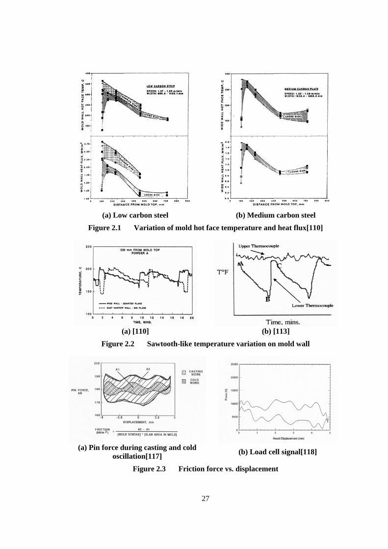
27

(a) Low carbon steel (b) Medium carbon steel

Figure 2.1 Variation of mold hot face temperature and heat flux[110]

(a) [110] (b) [113]

Figure 2.2 Sawtooth-like temperature variation on mold wall

(a) Pin force during casting and cold

oscillation[117] (b) Load cell signal[118]

Figure 2.3 Friction force vs. displacement

28

(a) CaO-SiO2-CaF2[123]

(b) CaO-SiO2-Al2O3[124]

29

(c) SiO2-Al2O3-Na2O[124]

(d) CaO-SiO2-Na2O[124]

Figure 2.4 Ternary phase diagrams showing liquidus temperature contours

30

Figure 2.5 Viscosity of some commercial silicate glasses[126]

31

(a) 45%CaO, 41%SiO2, 7%Al2O3, 7%Na2O

(b) 44.5%CaO, 44.5%SiO2, 4%Al2O3, 7%Na2O

(c) 39.6%CaO, 40.9%SiO2, 6.9%Al2O3, 9.6%Na2O

(d) 43~44%CaO, 43~44%SiO2, 7%Al2O3, 5~7%Na2O

Figure 2.6 TTT curves obtained by double thermocouple technique[145]

600

800

1000

1200

1400

1 10 100 1000 104 105

Tem

pera

ture

(o C)

Time (s)

CaO: 37.8%

SiO2: 33.3%

Na2O: 8.2%

Al2O

3: 7.9%

F: 8.4%

Fe2O

3: 1.7%

K2O: 0.6%

MgO: 0.6%

600

800

1000

1200

1400

1 10 100 1000 104 105

Tem

pera

ture

(o C)

Time (s)

CaO: 33.4%

SiO2: 39.5%

Al2O

3: 19.5%

MgO: 7.3%

(a) Typical crystalline slag[143] (b) Typical glassy slag[144]

Figure 2.7 TTT curves of typical crystalline and glassy slag

32

(a) Variation in heat transfer[157] (b) Friction force[16]

Figure 2.8 Effect of parameter η·Vc

Figure 2.9 Relation between slag properties and casting speed[158]

33

CHAPTER 3. MODEL DESCRIPTION AND VALIDATION

3.1 Steel Solidification Model

The model in this work computes 1-D transient heat flow through the solidifying

steel shell, coupled with 2-D steady-state heat conduction within the mold wall.

Superheat from the liquid steel was incorporated as a heat source at the steel solid/liquid

interface. The model features a detailed treatment of the interfacial gap, including mass

and momentum balances on the liquid and solid slag layers, friction between the slag and

mold, and slag layer fracture. The model simulates axial (z) behavior down a chosen

position on the mold perimeter. Wide-face, narrow-face and even corner simulations can

thus be conducted separately.

3.1.1 Superheat Delivery

Before it can solidify, the steel must first cool from its initial pour temperature to

the liquidus temperature. Due to turbulent convection in the liquid pool, this “superheat”

contained in the liquid is not distributed uniformly. A small database of results from a 3-

D fluid flow model[61] is used to determine the heat flux, qsh, delivered to the

solid/liquid interface due to the superheat dissipation, as a function of distance below the

meniscus. The initial condition of the liquid steel at the meniscus is then simply the

liquidus temperature.

Previous work[61] found that this “superheat flux” varies linearly with superheat

temperature difference and also is almost directly proportional to casting speed. The

34

superheat flux function in the closest database case is adjusted to correspond with the

current superheat temperature difference, ∆Tsup, and casting speed, Vc, as follows:

sup

sup

∆=

∆o c

sh sh o oc

T Vq qT V

(3.1)

where oshq is the superheat flux profile from the database case with conditions of superheat

temperature difference supoT∆ and casting speed o

cV . Further adjustments are made to

translate the heat flux peak to account for differences in nozzle configuration between the

current conditions and the database. Examples of the superheat flux function are included

in Figure 3.1, which represents results for a typical bifurcated, downward-directed

nozzle[61]. The influence of this function is insignificant to shell growth over most of the

wide face, where the superheat flux is small and contact with the mold is good.

3.1.2 Heat Conduction in the Solidifying Steel Shell

Temperature in the thin solidifying steel shell is governed by the 1-D transient

heat conduction equation, which becomes the following on applying the chain rule to the

temperature-dependent conductivity:

22*

2 ∂∂ ∂ρ∂ ∂ ∂

∂ ⎛ ⎞= + ⎜ ⎟∂ ⎝ ⎠steel

steel steel steelkT T TCp k

t x T x (3.2)

Temperature dependent properties for carbon steel are given in Appendix B[159].

Both sensible and latent heat of steel are included in the effective specific heat, *steelCp ,

explained in Section 3.1.5-C.

This equation assumes that axial (z) heat conduction is negligible in the steel,

which is reasonable past the top 10mm, due to the large advection component as

indicated by the large Péclet number:

35

0.0167 0.81 7400 670 2236.30

c mold steel steel

steel

V Z CpPekρ × × ×

= = = The simulation domain for

this portion of the model is a slice through the liquid steel and solid shell, which moves

downward at the casting speed, as pictured in Figure 3.1 and Figure A1 together with

typical interface conditions. At the internal solid/liquid steel interface, the “superheat

flux”, qsh, delivered from the turbulent liquid pool, (section 3.1.1), is imposed as a source

term. From the external surface of the shell, interfacial heat flux, qint, is lost to the gap,

which depends on the mold and slag layer computations, described in the following two

sections. Appendix A provides the explicit finite-difference solution of Eq.(3.2),

including both of these boundary conditions.

3.1.3 Microsegregation Model

The previous model uses the equilibrium Fe-C phase diagram to calculate steel

liquidus, solidus, peritectic temperature and phase fractions which include the influences

of Mn, Si, Al, S, P etc. 14 elements[8, 160]. To model realistic microsegregation during

solidification of steel, an analytical model[161] based on the Clyne-Kurz equation has

been added into CON1D. The non-equilibrium model is extended to take into account the

effect of multiple components, a columnar dendrite microstructure, coursing, and the δ/γ

transformation, which was developed by Won[161]. This model is implemented in this

work and applied to predict phase fractions during solidification, microsegregation of

solute elements, the solidus temperature and the secondary dendrite arm spacing. The

phase fractions are then used for calculating temperature dependent steel thermal

properties[159, 162]

36

Liquidus, solidus and peritectic temperatures depend on steel composition and

cooling rate, CR, as following:

0,= − ⋅∑liq pure i ii

T T m C (3.3)

( ), 0, , , , , 1= − ⋅ =∑sol pure i L i i R i i si

T T m C C C k D f (3.4)

,

δ γ δ γ δ δ= − ⋅ ⋅∑pure L i

Li i

iT T n k C (3.5)

Extended data needed for this model are listed in Table 3.1 and include the

partition coefficients, ki, diffusion coefficients, Di, for each phase, the slopes of the

equilibrium liquidus, mi, and the slopes of Ar4 lines, ni, for the pseudo-binary alloys of 14

elements with iron. The results are not very sensitive to cooling rate, as the

accompanying dendrite arm spacing change tends to compensate[161].

3.1.4 Ideal Taper

The narrow-face of the mold should be tapered to match the shrinkage of the steel

shell, which is cooling against the wide face. Previous work has determined that this

shrinkage depends mainly on the surface temperature of the shell and the steel grade[50]. The model predicts ideal average taper, by dividing the thermal strain, ε, by distance

down the mold (instantaneous taper) or by the mold length (total taper per m). Thermal

shrinkage strain is estimated here in two different ways, firstly εth1, by:

1 ( ) ( ) ε = −th sol sTLE T TLE T (3.6)

Another method to calculate shrinkage was developed by Dippenaar[73, 74]. The

strain εth2, is computed by summing the average thermal linear expansion of the solid

portion of the shell between each pair of consecutive time steps:

37

( ) ( )( )

20 1

1 ε +∆

= =

⎛ ⎞⎛ ⎞= −⎜ ⎟⎜ ⎟⎝ ⎠⎝ ⎠

∑ ∑t solid nodes

t t tth i i

t iTLE T TLE T

i (3.7)

Here, TLE is the thermal linear expansion function for the given steel grade, calculated

from weighted averages of the phases present. This model also includes the effect of

mold distortion, slag layer thickness and funnel mold extra length (if present). It has been

applied elsewhere to predict ideal taper[21]

3.1.5 Steel Properties

The program includes several different choices for steel properties, including

simple constants input by the user. By default, the liquidus temperature, solidus

temperature, phase fraction curve, thermal conductivity, specific heat and thermal linear

expansion are all calculated as functions of composition and temperature. Steel density,

ρsteel, latent heat, Lf, and steel surface emissivity, εsteel, are constants. For carbon steel:

ρsteel =7400kg/m3, Lf =271kJ/kg, εsteel =0.8

A. Phase Fraction

By default, equilibrium lever-rule calculations are performed on an Fe-C phase

diagram, whose phase field lines are specified as simple linear functions of alloy content

(including the influences of Si, Cr, Mn, Ni, Mo, Cu, Ti, P, S, Al, V, N, Nb and W)

reported by Kagawa[160] in order to calculate steel liquidus, solidus, peritectic

temperature and phase fractions. Alternatively, the user can choose a non-equilibrium

micro-segregation model[161] to find these values, which was extended in this work to

include the effects of 14 elements, given in Table 3.1. For a 0.044%C, 0.022%Mn,

0.006%S, 0.01%P, 0.009%Si 0.049%Al plain carbon steel, the equilibrium phase

diagram model calculates Tliq=1528oC, Tsol=1509oC, while with 10oC/second cooling rate,

38

the segregation model gives Tliq=1532oC, Tsol=1510oC. Figure 3.2 shows the solid

fraction temperature curve in the mushy zone obtained from both models. Both models

produce similar results. The surprising finding that the equilibrium model produces

slightly lower transformation temperatures shows that differences in the coefficients

which define the alloy-dependent equilibrium lines are more important than the non-

equilibrium effects due to segregation at the typical cooling rates, dendrite arm spacing,

and compositions considered.

B. Thermal Conductivity of Steel

The thermal conductivity of carbon steel is calculated as a function of

temperature, carbon content and phase fraction, which was fitted from measured data

compiled by K. Harste[159]. The specific functions are listed in Appendix B. Stainless

steel thermal conductivity is calculated according to the fitted equation based on

measured data compiled by Pehlke[162]. Figure 3.3 compares some typical plain-carbon

steel, austenitic-stainless steel and ferritic stainless steel conductivities. Thermal

conductivity of the liquid is not artificially increased, as common in other models,

because the effect of liquid convection is accounted for in the superheat flux function,

which is calculated by models[61] which fully incorporate the effects of turbulent flow.

C. Effective Specific Heat of Steel

Specific heat is calculated as a function of temperature, carbon content, phase

fraction and steel grade. Appendix B gives the specific heat functions for carbon steel,

found by differentiating the enthalpy curve from K. Harste[159]. Refer to Pehlke[162] for

the specific heat functions of stainless steel. When the steel temperature is between the

39

solidus and liquidus temperatures, latent heat, Lf, is evolved using the liquid phase

fraction curve found previously. The effective specific heat is then defined as:

* = = − sp p f

dfdHC C LdT dT

(3.8)

Figure 3.4 shows the specific heat curve of AISI 1026 carbon steel using the

micro-segregation model compared with measured data[162]. The curves for other alloys,

such as used later, are similar except for within the mushy region. So long as it properly

matches the total latent heat, its exact shape has little effect on shell growth or surface

temperature.

D. Thermal Linear Expansion of Steel

By default, the thermal linear expansion, TLE, needed for shrinkage and ideal

taper calculations is computed as a function of steel density,

( )0

3 1ρρ

= −TLET

(3.9)

where ρ0=ρsteel. The composition and temperature-dependent steel density function for

carbon steel, ρ(T) is taken from measurements tabulated by Harste[159] and is listed in

Appendix B. Constant density, ρsteel is adopted for the heat flow calculations in order to

enforce constant mass in the fixed-domain computation.

Alternatively, the user may input a thermal linear expansion coefficient, α, so:

( )α= −TLE T Tsol (3.10)

This is done for stainless steel, where α is taken from Pehlke[162].

40

3.1.6 Steel Solidification Model Validation

The solidification model is verified here through comparison with an analytical

solution for 1-D heat conduction with phase change[163]. This solution assumes constant

shell surface temperature and constant steel properties. Table 3.2 lists the constants used

in both the analytical solution and the CON1D validation case, which are chosen for

typical conditions expected in practice. The difference between the steel liquidus and

solidus temperatures is only 0.1oC to approximate the single melting temperature

assumed in analytical solution, which is set to the mean of Tliq and Tsol used in CON1D.

The pour temperature is set to the liquidus because superheat is neglected in the

analytical solution. For the CON1D model, the time step size ∆t is 0.004second and node

spacing is 0.5mm.

Figure 3.5 compares results from the analytical solution and CON1D for (a) the

temperature distribution through the shell at different times and (b) the growth of shell

thickness with time. The results show that the predictions of the CON1D model is very

accurate, so the same time step and mesh size are used in the following cases.

3.2 Heat Transfer and Mass Balance in Slag

3.2.1 Heat transfer Across the Interfacial Gap

Heat transfer across the interfacial gap governs the heat flux leaving the steel, qint,

to enter the mold. To calculate this at every position down the mold, the model evaluates

an effective heat transfer coefficient, hgap, between the surface temperature of the steel

shell, Ts, and the hot face of the mold wall, Tmold:

( )int = −gap s moldq h T T (3.11)

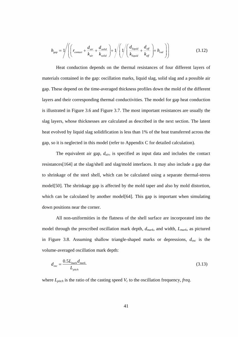
41

1 1 1⎛ ⎞⎛ ⎞⎛ ⎞⎛ ⎞⎜ ⎟= + + + + +⎜ ⎟⎜ ⎟⎜ ⎟ ⎜ ⎟⎜ ⎟⎜ ⎟⎝ ⎠ ⎝ ⎠⎝ ⎠⎝ ⎠

liquid effair solidgap contact rad

air solid liquid eff

d dd dh r hk k k k

(3.12)

Heat conduction depends on the thermal resistances of four different layers of

materials contained in the gap: oscillation marks, liquid slag, solid slag and a possible air

gap. These depend on the time-averaged thickness profiles down the mold of the different

layers and their corresponding thermal conductivities. The model for gap heat conduction

is illustrated in Figure 3.6 and Figure 3.7. The most important resistances are usually the

slag layers, whose thicknesses are calculated as described in the next section. The latent

heat evolved by liquid slag solidification is less than 1% of the heat transferred across the

gap, so it is neglected in this model (refer to Appendix C for detailed calculation).

The equivalent air gap, dair, is specified as input data and includes the contact

resistances[164] at the slag/shell and slag/mold interfaces. It may also include a gap due

to shrinkage of the steel shell, which can be calculated using a separate thermal-stress

model[50]. The shrinkage gap is affected by the mold taper and also by mold distortion,

which can be calculated by another model[64]. This gap is important when simulating

down positions near the corner.

All non-uniformities in the flatness of the shell surface are incorporated into the

model through the prescribed oscillation mark depth, dmark, and width, Lmark, as pictured

in Figure 3.8. Assuming shallow triangle-shaped marks or depressions, dosc is the

volume-averaged oscillation mark depth:

0.5= mark mark

oscpitch

L ddL

(3.13)

where Lpitch is the ratio of the casting speed Vc to the oscillation frequency, freq.

42

The oscillation marks affect heat transfer in two different ways. Firstly, the

oscillation marks consume mold slag, so affect the slag layer thicknesses, as described in

next section. Secondly, they reduce heat conduction by effectively providing an extra

gap. This extra gap is represented by deff, calculated based on a heat balance[31] which

produces the same total heat flux as found by combining the heat fluxes across the two

parallel conduction paths (at or adjacent to the oscillation mark), averaged spatially (z-

direction) using an appropriate weighted average:

( )0.5

1 0.5=

⎛ ⎞− + +⎜ ⎟⎜ ⎟+⎝ ⎠

mark markeff

gapmarkpitch mark mark

liquid solid mark

L ddkdL L L

d d k

(3.14)

( ) _1⎛ ⎞⎛ ⎞

= + + +⎜ ⎟⎜ ⎟⎜ ⎟⎜ ⎟⎝ ⎠⎝ ⎠

liquidsolidgap liquid solid rad liquid

solid liquid

kdk d d hk d

(3.15)

The oscillation marks are assumed to be filled with either slag, air, or a mixture,

depending on the local shell surface temperature. This governs the value of kmark.

Except for perhaps a microscopically thin glassy surface layer, experience has

shown that the cold slag layer adjacent to the mold wall is usually crystalline[142, 165],

and thus opaque. Thus, radiation occurs only across the semi-transparent hot glassy or

liquid layer above Tfsol[137, 166], according to Eq.(3.16), as shown in Figure 3.6:

( )( )( )

( )2 2 2

1 10.75 1

σ

ε ε

+ += <

+ + + −

s K fsol K s K fsol Krad mold fsol

liquid effslag steel

m T T T Th T T

a d d (3.16)

where m is slag refractive index; TsK and Tfsol K are Ts and Tfsol expressed in Kelvin, a is

average absorption coefficient of the slag, assuming graybody radiation (εslag =0.9). If the

liquid slag runs out, so that s fsolT T< , then hrad=0. In the unlikely event that

mold fsolT T≥ ,

43

εslag would be replaced by εmold, and Tfsol by Tmold in Eq.(3.16). Jenkins showed that this

simple equation to characterize radiation with absorption across a gap, Eq.(3.16), is

accurate to within 10% relative to a full multi-view factor analysis including radiation-

conduction[82]. This is sufficiently accurate because the radiation component itself

usually contributes only on the order of 10% of the gap heat transfer.

3.2.2 Mass and Momentum Balance on Powder Slag Layers

Slag is assumed to flow down the gap as two distinct layers: solid and liquid. The

solid layer is assumed to move at a time-average velocity, Vsolid, which is always between

zero and the casting speed, Vc, according to the input solid slag speed ratio, fv.

= ⋅solid v cV f V (3.17)

The downward velocity profile across the liquid slag layer is governed by the

simplified Navier-Stokes equation, assuming laminar Couette flow:

( )x xµ ρ ρ∂∂ ⎛ ⎞ = −⎜ ⎟∂ ∂⎝ ⎠

zsteel slag

V g (3.18)

A small body force opposing flow down the wide face gap is created by the

difference between the ferrostatic pressure from the liquid steel, ρsteel g, transmitted

through the solid steel shell, and the average weight of the slag, ρslag g. The time-average

velocity of the liquid slag described by Eq.(3.18), Vz, is subjected to boundary conditions

constraining it to the casting speed, Vc on its hot side and to the solid slag velocity, Vsolid

on its cold side.

The temperature dependent viscosity of the liquid slag is fit to a simple power-law

relation, which better represents low-temperature high-viscosity behavior than a simple

Arrhenius equation[99]:

44

µ µ⎛ ⎞−

= ⎜ ⎟⎜ ⎟−⎝ ⎠

n

o fsolo

fsol

T TT T

(3.19)

where the parameters Tfsol and n are chosen empirically to fit measured data and µo is the

viscosity measured at the reference temperature, To, usually chosen to be 1300oC. Using

only few important slag properties, Tfsol, µ1300, and an empirical index n, this equation

reasonable models the entire viscosity curve, and also enables an analytical solution for

slag flow in the gap as derived in the following sections. A typical curve obtained with

this function is shown in Figure 3.9 together with the measured viscosities by Lanyi that

it was fit to match[100]. Mold slags in service absorb some Al2O3 from the steel, which

changes their properties, including decreasing the solidification temperature[100, 151].

The second curve in Figure 3.9 was constructed for a reported solidification temperature

Tfsol of 1045oC and viscosity at 1300oC of 1.1Poise, and was used later in model

calibration.

By approximating temperature across the gap to vary linearly, Eq.(3.17) through

Eq.(3.19) can be solved for the time-averaged velocity distribution across the slag layers,

which is illustrated in Figure 3.7. Integrating across the liquid region yields an average

velocity for the liquid layer, liquidV :

( )( ) ( )

( )( )

2

2

122 3

ρ ρ

µ

− + += +

++ +liquidslag steel c solid

liquid

s

gd V V nV

nn n (3.20)

where µs is the slag viscosity at liquid layer/steel shell interface. A mass balance was

imposed to match the measured (known) powder consumption, Qslag(kg/m2), with the

total molten slag flow rate past every location down the interfacial gap, neglecting the

carbon content component, which burns off. This consumption rate is expressed as mass

45

of slag per unit area of the strand surface, which can be found from the consumption per

mass of product, Mslag(kg/ton) :

( ) ( ) ( )2/ /

2ρ ×

= × ×+slag slag steel

W NQ kg m M kg tonW N

(3.21)

where W is slab width and N is slab thickness. Slag can be carried downward by the solid

layer, the liquid layer, and in the oscillations marks:

ρ×

= + +slag csolid solid liquid liquid c osc

slag

Q VV d V d V d (3.22)

The liquid and solid layer thicknesses are obtained by solving a fourth order

polynomial equation found by combining Eq.(3.12) and Eq.(3.22). The transport of slag

by the oscillation marks depends on the lubrication state, discussed next.

Three different regions are distinguished down the mold, according to the

lubrication condition. Close to the meniscus, a solid slag rim exists against the mold wall.

Its thickness profile must be specified, as it depends on transient phenomena not yet in

the model.

The second region, shown in Figure 3.7, allows the solid slag layer to move at the

slow time averaged velocity Vsolid. It always also includes oscillation marks filled with

molten slag and a continuous liquid slag layer, which remains present so long as the outer

surface temperature of the steel Ts’ exceeds the slag solidification temperature, Tfsol:

'int= − ⋅ eff

s smark

dT T q

k (3.23)

Slag in the oscillation marks remains liquid longer, due to the higher local shell

temperature at their roots, Ts. Once the oscillation mark roots cool below the slag

solidification temperature, however, the slag entrapped in them solidifies. This defines

46

the third region, which consists of totally solid slag, moving downward at the uniform

speed, Vsolid. The oscillation marks no longer transport slag, so become filled with air.

The transition between the second and third regions is gradual.

3.3 Lubrication and Friction Model in Gap

It is important to emphasize that the above interfacial heat transfer model

represents steady, time-averaged behavior only. To investigate transient phenomena, a

transient version of this model is developed in this work to calculate liquid flow and solid

slag stress during the oscillation cycle, which is applied to predict transient shear stress,

friction, slip and fracture of the slag layers. Figure 3.10 shows the domain used in this

transient model. Table 3.3 gives the typical casting conditions and simulation parameters

used in model validation.

3.3.1 Liquid Slag Layer Flow Model

For simplicity, the slag is treated as two layers each with variable thickness in the

vertical (z-) direction: a rigid solid layer and a laminar liquid layer with temperature

dependent viscosity. A schematic profile of the mold, slag and steel shell velocities is

shown in Figure 3.11 for the case when the solid slag layer is stuck to the mold wall so its

average downward velocity, Vs, is zero. The steel shell moves downward at the casting

speed Vc, and the mold oscillates in the vertical direction with the sinusoidal

displacement function:

( )0 sin 22

π= +msZ Z ft (3.24)

47

A mass balance on the liquid slag layer gives the following continuity equation,

assuming incompressible flow, constant density and identical behavior within any

vertical slice, so velocity across the slab width, Vy is zero:

0∂ ∂+ =

∂ ∂x zV V

x z (3.25)

The following Navier-Stokes equation characterizes the laminar viscous flow of

liquid slag vertically within the gap:

ρ

ττ τ ρ

⎛ ⎞∂ ∂ ∂ ∂⋅ + ⋅ + ⋅ + ⋅⎜ ⎟∂ ∂ ∂ ∂⎝ ⎠

∂∂ ∂∂= − + + + +

∂ ∂ ∂ ∂

z z z zslag x y z

yzxz zzslag

V V V VV V Vt x y z

P gz x y z

(3.26)

In the horizontal direction, the internal pressure, P, is assumed to equal the

ferrostatic pressure, which is transmitted directly across the steel shell, so:

ρ∂=

∂ steelP gz

(3.27)

This is reasonable everywhere except near the corners that support themselves and near

the meniscus where pressure fluctuates. Thus, this model is appropriate within most of

the gap over the unsupported wide faces of slab casting.

In Eq.(3.26), zy

VVy

∂∂

and yz

yτ∂

∂ can be neglected because Vy=0. The three terms

zslag x

VVy

ρ ∂∂

, zslag z

VVz

ρ ∂∂

and zzz

∂∂τ are shown to be negligible in the next section for

typical continuous casting conditions. Thus Eq.(3.26) simplifies to the following as

gravity and downward viscous drag by the steel shell must balance the upward squeezing

from the ferrostatic pressure:

48

( )τρ ρ ρ∂∂⋅ = + −

∂ ∂xzz

slag slag steelV gt x

(3.28)

Shear stress in the liquid slag layer depends on the velocity gradient at each point

across the channel:

τ µ ∂=

∂z

xzVx

(3.29)

Setting temperature at the hot liquid layer side, Ts’, as the reference temperature,

Eq.(3.19) is rewritten as:

'

µ µ⎛ ⎞−

= ⎜ ⎟⎜ ⎟−⎝ ⎠

n

s fsols

fsol

T TT T

(3.30)

Assuming that temperature across the liquid slag layer thickness is linear gives:

( )'= − +s fsol fsoll

xT T T Td

(3.31)

Substituting Eq.(3.31) into Eq.(3.30) and replacing the viscosity term in Eq.(3.29)

with this position dependent viscosity yields:

τ µ ∂=

∂

nl z

xz s n

d Vx x

(3.32)

Differentiating Eq.(3.32) and substituting into Eq.(3.28), yields the following

momentum equation, governing the velocity distribution in the liquid film:

( )2

2 1ρ µ µ ρ ρ+

∂ ∂ ∂= − + −

∂ ∂ ∂

n nl lz z z

slag s s slag steeln n

d ndV V V gt x x x x

(3.33)

Differentiating Eq.(3.24) to get mold velocity Vm, and assuming the solid slag is

attached to the mold wall, the boundary conditions for the liquid slag layer model,

Eq.(3.33), are:

( )0solid/liquid slag layer interface: cos 2π π= = = = ⋅z x s mV V V sf ft (3.34)

49

liquid slag/steel shell interface: = =lz x d cV V (3.35)

Neglecting zVt

∂∂

and applying the boundary conditions Eqs.(3.34) and (3.35),

Eq.(3.33) can be integrated to obtain the following “pseudo-transient” analytical solution:

( )( )

( ) ( )( )

2 1

2 2ρ ρ ρ ρ

µ µ

+ +⎛ ⎞− − −−⎜ ⎟= + + +⎜ ⎟+ +⎝ ⎠

n nslag steel slag steel lc s

z sn ns l l s l

gx gdV V xV Vn d d n d

(3.36)

3.3.2 Liquid Slag Layer Flow Model Validation

To check the validity of the assumptions made to obtain Eq.(3.36), a fully

transient numerical solution was obtained using an explicit finite-difference discretization

of Eq.(3.33) with a central difference scheme:

( )

( ) ( )

1( ) ( ) 1( ) 1( ) 1( )

2 1

2

i t t i tz z

slag

n ni t i t i t i t i tl lz z z z z

s s slag steeln n

tV V

d ndV V V V V gx x x x

ρ

µ µ ρ ρ

+∆

+ − + −

+

∆= +

⎛ ⎞− + −− + −⎜ ⎟∆ ∆⎝ ⎠

(3.37)

A MATLAB[167] program was coded to solve this equation with boundary

conditions Eqs.(3.34) and (3.35) at different z-distances. Table 3.4 gives the parameters

of 4 cases used in the MATLAB program. Cases (a)-(b) are based on heat transfer results

for typical casting conditions as shown in Table 3.3; and Cases (c)-(d) use an extremely

thick liquid layer (2mm) from Chavez’s work[95]. Discretizing the continuity equation

Eq.(3.25) and processing the results at different z-distances (specifically z=53mm and

z=54mm for case (b)) allow computations of the other terms in Eq.(3.26).

Table 3.5 shows values of the different terms in Eq.(3.26) for case (b) at t=0.18s,

x=0.16mm. Note that zslag x

VVx

ρ ∂∂

, zslag z

VVz

ρ ∂∂

and zzz

∂∂τ are negligible compared to the

50

other terms. Also note that the transient term zslag

Vt

ρ ∂∂

contributes less than 1.5%, so can

justifiably be neglected too.

Figure 3.12 shows typical velocity profiles computed with these models. For

constant viscosity and a thin liquid layer, Figure 3.12(a), the velocity profiles are linear.

Otherwise, nonlinearity is significant. Figure 3.12 also compares the numerical solution

and the pseudo-transient analytical solution. It shows that the transient effect is negligible

for a film thickness of 0.2mm. Even for an extreme case, 2mm thick liquid film, Figure

3.12(c), (d), the maximum transient effect is barely perceptible. Therefore the pseudo-

transient analytical solution to the liquid slag layer flow equation, Eq.(3.36) is a

reasonable approximation of the full transient solution.

Substituting Eq.(3.36) into Eq.(3.32) gives:

( ) ( ) ( ) ( ) ( )( )1 212

ρ ρµτ

− + − ++ −= +

+slag steel ls c s

xzl

g n d n xn V Vd n

(3.38)

Evaluating Eq.(3.38) at x=dl gives the shear stress at the slag/steel interface when

a liquid slag layer is present:

( ) ( ) ( )( )/

12

ρ ρτ µ

−+ −= −

+slag steel lc s

liquid flux steel sl

gdn V Vd n

(3.39)

3.3.3 Solid Slag Layer Stress Model

Near the meniscus, the solid slag layer attaches to the mold wall and oscillates

with the mold. However, if the solid slag layer breaks, and where it breaks, could greatly

affect heat transfer across the gap. A stress model is developed to investigate force

balances and possible fracture in the solid slag layer.

51

The equilibrium force balance in the axial z-direction is:

0τ σ∂ ∂+ + =

∂ ∂xz z

zFx z

(3.40)

Knowing that body forces Fz are negligible in the solid layer, Figure 3.13

illustrates the force balance in a solid slag layer discretization element cut from Figure

3.10 for four typical cases. Evaluating τxz in Eq.(3.38) at x=0 gives the shear stress

boundary condition at the interface between the liquid and solid slag layers:

( ) ( )( ) ( )( ) ( )/

1 12

τ µ ρ ρ+ − +

= + −+

c ss l s slag steel l

l

n V V t ngd

d n (3.41)

Note that this shear stress varies greatly during the oscillation cycle.

The maximum shear stress transmitted to the mold by Coulomb friction with the

solid slag layer, due to relative motion of the mold and shell is:

τ φ σ= ⋅max static x (3.42)

The normal stress, σx, comes from the liquid steel ferrostatic pressure and the

liquid slag pool above the meniscus, which generates a tiny additional head:

( )0σ ρ ρ= − +x slag steelgh gz (3.43)

Shear stress must be continuous across the gap, including both the boundaries at

the mold and steel shell surfaces. When the liquid layer/steel interface shear stress is

smaller than the maximum solid contact shear stress, then the friction force drops to

match it, as shown in Figure 3.13(a). In this “liquid shear stress limited” case, Figure

3.13(a), the friction force is less than the maximum possible static friction given in

Eq.(3.42). Ferrostatic pressure then generates axial stress σz in the solid layer that is

compressive:

52

1υσ σ

υ= −

−z x (3.44)

so xz-shear stress at the mold side can be calculated from Eqs.(3.40), (3.43), and (3.44)]

as follows:

/ /0

/1

υτ σ τ ρ τυ=

= − ⋅ + = +−∫

sd

mold z s l steel s s lx

d dz dx gd (3.45)

Alternatively, if the liquid layer shear stress is larger than the maximum static

friction, mold maxτ τ= , then axial stress develops in the solid layer to compensate. In order

to satisfy the force balance Eq.(3.40):

/σ τ= − ⋅z xzd d dz dx (3.46)

Discretizing Eq.(3.46) axially, and integrating across the thickness, the axial stress

in the solid slag layer at z+∆z is:

/τ τσ σ+∆

−= − ∆max s l

z z zs

zd

(3.47)

Specifically, axial stress is tensile during the up-stroke and compressive in the

down-stroke for this “mold friction limited” case shown in Figure 3.13(b). Furthermore,

the axial tension accumulates over successive slices of the solid slag layer. The shear

stress transmitted to the mold wall is the minimum of the maximum static friction stress

and the solid/liquid interface stress:

/ ,1

υτ ρ τ τυ

⎛ ⎞= +⎜ ⎟−⎝ ⎠mold steel s s l maxmin gd (3.48)

3.3.4 Solid Slag Layer Stress Model Validation

To validate the stress model of the solid slag layer, a simplified case was solved

using elastic finite-element stress analysis with ANSYS[168]. Figure 3.14 shows the

53

ANSYS model domain and mesh. The boundary condition at the mold side had

displacements fixed to zero and at the liquid side was normal ferrostatic pressure, xσ ,

from Eq.(3.43) and tangential shear stress, /s lτ (from CON1D). Table 3.3 gives the input

conditions and simulation parameters used in CON1D. Figure 3.15 compares the stress

results from ANSYS and CON1D using Eqs.(3.47) and (3.48) and assuming the solid

slag layer is stably attached to the mold wall. The CON1D model matches ANSYS

except within 10mm near mold exit, where the real axial stress must quickly tend to zero

(to match ambient atmospheric pressure).

3.3.5 Solid Slag Layer Fracture Model

If the axial stress exceeds the fracture strength, the solid slag layer will break, and

be dragged down the mold wall. The shear stress on the mold/slag interface for this

condition is:

τ φ σ= ⋅mold moving x (3.49)

Substituting Eqs. (3.41) and (3.49) into Eq.(3.45) can solve for the solid layer

velocity Vs after it detaches from the mold wall. Fracture and sliding of the solid slag

layer tend to create a gap between the upper attached solid layer and the lower moving

layer. This gap may re-fill with liquid slag, and the solid layer might re-attach to the mold

wall when the instantaneous velocity of the oscillating mold wall equals the moving solid

slag layer velocity. The time for the liquid slag to fill the gap and the solid slag to re-

attach depends on the slag consumption rate and liquid slag fluidity. The fracture and

filling process requires extra slag consumption, which decreases the liquid layer thickness

and increases shear stress(/friction) for the whole mold.

54

3.3.6 Mold Friction

The friction measured in operating casting molds may come from mold/slag

contact, excessive taper, misalignment or a combination of the three.

A. Slag-layer friction

Previous research has suggested that friction against the slag layer is

important[103]. The liquid slag-layer flow model and solid slag-layer stress model

described in this work give the shear stress on the mold wall, moldτ , due to mold/slag

contact. Integrating the shear stress over the mold face gives the total friction force due to

contact between the mold and slag layers:

02( )τ= ⋅ + ⋅∫

moldZ

contact moldF W N dz (3.50)

where, Zmold: working mold length; W: slab width; N: slab thickness.

This model has been incorporated into CON1D, and is used for the study

described in later chapters.

B. Excessive taper

If the solid slag layer remains attached to the mold wall all the way down the

mold, there will be a continuous, thick liquid slag layer (to provide slag consumption)

and a thick solid slag layer, leading to low heat transfer across the mold/shell gap. Then

the shell will have relatively high surface temperature and small shrinkage. In this case,

excessive narrow face taper may squeeze the steel shell and therefore lead to increased

friction. The maximum force from squeezing the shell occurs if the shell buckles, leading

to longitudinal surface depressions, such as off-corner gutter in extreme cases[20], as

55

shown in Figure 3.16. Applying the Eular critical buckling load equation with rigid ends

yields an estimate of the normal stress on the mold wall, Fcr:

2 2 3

2 2

4 412

π π= =cr

eff eff

EI E b hFL L

(3.51)

Where, b is the shell thickness, h is the vertical contact length along the narrow face, Leff

is the unsupported shell width across the wide face from the corner and E is the effective

elastic modulus of the hot steel shell. So the friction due to buckling for each narrow face

is:

2φ= ⋅excessive taper static crF F (3.52)

C. Excessive taper

Misalignment of the mold and strand is another important potential cause of

friction. The friction force during each oscillation cycle is inferred from the difference

between the force transducer measurements with and without molten steel in the

mold[169]. Currently, such friction signals can be used to monitor and detect

misalignment problems in operating casters.

3.4 Mold Heat Transfer Model

3.4.1 Heat Conduction in the Mold

Two dimensional, steady state temperature within a rectangular vertical section

through the upper portion of the mold is calculated assuming constant conductivity:

2 2

2 2+ = 0 ∂ ∂∂ ∂

T Tx z

(3.53)

56

This equation is solved using a standard Fourier series product solution[170]

applying fixed heat flux, int moldTq k x

∂= − ∂ , and convection, hwater and Twater as boundary

conditions, as shown in Figure 3.17(a) (refer to Appendix D[171]). This copper domain is

generally chosen to extend from the top of the mold to 100mm below the meniscus.

Below this meniscus region, heat flow is one-dimensional through the thickness.

Temperature at the copper hot face, Thotc, is then:

int1 +

⎛ ⎞= + ⎜ ⎟

⎝ ⎠mold

hotc waterwater mold

dT T qh k

(3.54)

where dmold is the copper mold thickness calculated in Appendix E[171]. Coating layers

and air gap are incorporated as needed to find the mold hot face temperature, Tmold, by

adding extra dcoat/kcoat and dair/kair resistances to Eq.(3.54) as needed. In addition to the

heat flux across the interface, qint, this calculation requires the initial cooling water

temperature, Twater, input as a boundary condition, and the effective water heat transfer

coefficient, hwater, discussed next.

3.4.2 Convection to the Cooling Water

The effective heat transfer coefficient between the cooling water and the cold face

(“water-side”) of the mold, hwater, is calculated including a possible resistance due to scale

deposits on the surface of the cooling water channels:

11⎛ ⎞

= +⎜ ⎟⎜ ⎟⎝ ⎠

scalewater

scale fin

dhk h

(3.55)

To account for the complex nature of heat flow in the undiscretized width

direction of the mold, the heat transfer coefficient between the mold cold face and the

57

cooling water, hfin, incorporates heat flow to both the root and sides of the water channels,

the latter treated as heat-transfer fins.

( )( )

22 2tanh

−= +

−chw mold ch ch ww ch

finch ch mold ch ch

h k L w h dh whL L k L w

(3.56)

where the mold geometry parameters, Lch, wch, and dch are shown in Figure 3.17(b). The

heat transfer coefficient between the water and the sides of the water channel, hw, is

calculated assuming turbulent flow through an equivalent-diameter pipe using the

empirical correlation of Sleicher and Reusse[172], which is reported[173] to be more

accurate than other relations such as Dittus and Boelter[174]:

( )1 25 0.015Re Pr= + c cwaterw waterf waterw

khD

(3.57)

where 2 ch ch

ch ch

w dDw d

=+

is the equivalent diameter of the water channel,

( )1 0.88 0.24 4 Prwaterwc = − + , 0.6Pr2 0.333 0.5 waterwc e−= + are empirical constants. The water

properties could be constants specified by user input, or they are calculated based on the

bulk temperature in cooling channel and wall temperature at mold cold face accordingly,

as given in Appendix F[171]

The presence of the water slots can either enhance or diminish the heat transfer,

relative to a plate-shaped mold wall with uniform thickness, dmold, such as used in billet

casting. Deep, closely spaced slots augment the heat transfer coefficient, (hfin larger than

hw) while shallow, widely spaced slots inhibit heat transfer. In most molds, hfin and hw are

very close.

Although it slightly underpredicts mold temperature, Eq.(3.56) was shown,

through comparison with many 3-D computations for a variety of typical slab casting

58

mold geometries and conditions, to match the temperature within 1% at the water slot

root and from 0.1% to 6% at the hot face [31, 175]. For a typical hot face temperature of

190oC and water temperature of 30oC, it gives maximum errors of 2oC and 10oC. It is

most accurate for molds with either deep, closely-spaced slots[31] or very wide

slots[175], where cold face temperature is most nearly constant as assumed in Eq.(3.56).

3.5 Spray Zones

The secondary cooling zones begin right after the mold exit and are divided into

different zones according to the different support roll diameter or different cooling water

flow rates from spray nozzles, which are assumed in the middle between two rolls, as

shown in Figure 3.18(a). Heat flux from the strand surface varies greatly between each

pair of support rolls according to spray nozzle cooling (based on water flux), hspray;

radiation, hrad_spray; natural convection, hconv; and heat conduction to the rolls, hroll, as

shown in Figure 3.18(b). Incorporating these phenomena enables the model to simulate

heat transfer during the entire continuous casting process. The heat extraction due to

water sprays is a function of water flow[176], of the following form:

( )1= ⋅ ⋅ − ⋅cspray water sprayh A Q b T (3.58)

where Qwater (l/m2s) is water flux in the spray zones, and Tspray is the temperature of the

spray cooling water. In Nozaki’s empirical correlation[177], A=0.3925, c=0.55,

b=0.0075, which has been used successfully by other modelers[176, 178].

Radiation is calculated by:

( )( )2 2_ σ ε= ⋅ + +rad spray steel s K amb K s K amb Kh T T T T (3.59)

59

where Tamb is ambient temperature, TsK and TambK are Ts and Tamb expressed in Kelvin.

Natural convection is treated as a constant input for every spray zone. For water-cooling

only, it is not very important, so was simplified to 8.7W/m2K everywhere. Larger values

can be input for hconv to reflect the stronger convection when there is air mist in the

cooling zone. Heat extraction into the rolls is calculated based on the fraction of heat

extraction to the rolls, froll, which is calibrated for each spray zone:

( )( )( ) ( )

_

_1

⎛ ⎞+ + ⋅ +⎜ ⎟=⎜ ⎟⋅ − + ⋅ − −⎝ ⎠

rad spray conv spray sprayrollroll

roll contact roll rad spray conv spray pitch spray roll contact

h h h LfhL f h h L L L

(3.60)

Heat extraction is a maximum directly beneath the spray nozzle (assumed

centered between the rolls) and at the roll/shell contact region. The relative size of this

maximum is governed by the fraction of heat specified to leave relative to that removed

by the spray cooling water. A typical froll value of 0.05 produces local temperature drops

beneath the rolls of about 100oC. Beyond the spray zones, heat transfer simplifies to

radiation and natural convection.

3.6 Solution Methodology

The model requires simultaneous solution of three different systems of equations:

1-D transient heat conduction and solidification of the steel shell, 2-D steady state heat

conduction in the mold, and the equations balancing heat, mass, momentum and stress in

the gap. The simulation starts by setting the initial steel and mold temperatures to the

pouring temperature and inlet cooling water temperature respectively. Phase

transformation temperatures and phase fraction temperature curves are then calculated,

using either equilibrium phase diagram or microsegregation model. Then, each time step

begins by rearranging and solving Eqs.(3.12) and (3.22) simultaneously for dliquid and

60

dsolid, based on heat and mass balances at the previous time step. The heat flux qint is then

calculated according to Eqs.(3.11) and (3.12), which is the boundary condition for both

steel and mold domains. The heat transfer coefficient, hwater is calculated according to

cooling channel conditions with Eqs.(3.55) to (3.57), and used to obtain mold

temperatures. Applying the superheat flux boundary condition, Eq.(3.1), as an internal

heat source at the steel solid/liquid interface, the model uses an explicit, central-finite

difference algorithm originally developed by Pehlke[179] to solve Eq.(3.2) for the shell

temperature at each time step (Appendix A). This limits the maximum time step size, ∆t.

When a node temperature drops below the liquidus temperature, its solid fraction is

calculated from the latent heat evolved, and then the node temperature is adjusted[180]

(Eq.(A6)) according to the phase fraction-temperature curves, described in Section 3.1.5-

A. The results are used as initial conditions for the 2-D mold calculation, which solves

Eq.(3.53) analytically (Appendix D[171]), relating distance down the mold, z, to time in

the shell through the casting speed. Subsequently, the entire 1-D shell solidification

model in the 2-D mold region is recomputed using the new 2-D mold temperatures as its

boundary condition. This stepwise coupling procedure alternates between models until

the 1-D mold temperatures converge to match the 2-D results within 3oC. This produces a

self-consistent prediction, which is stable for almost all coupled simulations investigated

and usually converges in 3-4 iterations.

Nest the model calculates velocity and shear stress distribution in the liquid slag

layer (Eq.(3.36)) based on the temperature distribution solved by Eq.(3.31). Solving the

force balance equation in the solid layer, Eq.(3.40), gives the axial stress, which is used to

decide if the solid layer fractures. The friction force on the mold wall is obtained finally

61

by integrating the shear stress over the whole mold faces (Eq.(3.50)). Figure 3.19 gives a

flow chart of the whole procedure.

The model has been incorporated into a user-friendly FORTRAN program,

CON1D[171]. A 100-second long simulation with 0.004sec time step and 100-node mesh

runs on a Pentium III personal computer (using 3.1Mbytes of memory) in about 30

seconds. Appendix I gives the sample input and output files of CON1D version7.5.


Table 3.1 Equilibrium Partition Coefficient, Diffusion Coefficient,

and Liquidus Line Slopes of the Solute Elements

Element kδ/L kγ/L Dδ (cm2/sec) Dγ (cm2/sec) m (oC/%) n (oC/%)

C 0.19 0.34 0.0127exp(-19450/RT) 0.0761exp(-32160/RT) 78.0 -1122

Si 0.77 0.52 8.0exp(-59500/RT) 0.3exp(-60100/RT) 7.6 60

Mn 0.76 0.78 0.76exp(-53640/RT) 0.055exp(-59600/RT) 4.9 -12

P 0.23 0.13 2.9exp(-55000/RT) 0.01exp(-43700/RT) 34.4 140

S 0.05 0.035 4.56exp(-51300/RT) 2.4exp(-53400/RT) 38.0 160

Cr 0.95 0.86 2.4exp(-57310/RT) 0.0012exp(-52340/RT) 1.04 13.4

Ni 0.83 0.95 1.6exp(-57360/RT) 0.34exp(-67490/RT) 4.69 -28.6

Cu 0.53 0.88 2.6exp(-57360/RT) 0.7exp(-68350/RT) 5.32 -10.4

Mo 0.80 0.585 3.47exp(-57690/RT) 0.068exp(-59000/RT) 2.6 77.6

Ti 0.38 0.33 3.15exp(-59200/RT) 0.15exp(-59980/RT) 10.24 120.5

V 0.93 0.63 4.8exp(-57360/RT) 0.284exp(-61900/RT) 12.95 85.5

Nb 0.40 0.22 50.2exp(-60220/RT) 0.83exp(-63690/RT) 10.24 70.8

W 0.85 0.45 1.57exp(-58200/RT) 0.13exp(-57300/RT) 0.24 18.8

N 0.25 0.48 0.008exp(-18900/RT) 0.91exp(-40270/RT) 60.0 -

Note: R is gas constant of 1.987cal/mol K, and T is temperature in Kelvin.

62

Table 3.2 Constants Used in Analytical Solution and

Validation Casefor Steel Solidification Model

Conductivity, ksteel 30.0 W/mK

Specific Heat, Cpsteel 670.0 J/kgK

Latent Heat, Lf 271.0 kJ/kg

Density, ρsteel 7400.0 kg/m3

Melting Temperature, Tmelt 1509.05 oC

Liquidus Temperature, Tliq 1509.1 oC

Solidus Temperature, Tsol 1509 oC

Shell Surface Temperature, Ts 1000 oC

63

Table 3.3 Typical Casting Condition and Simulation

Parameters for Transient Interfacial Gap Model

Carbon Content, C% 0.05 %

Liquidus Temperature, Tliq 1529 oC

Solidus Temperature, Tsol 1509 oC

Steel Density, ρsteel 7400 kg/m2

Fraction Solid for Shell Thickness Location, fs 0.3 - Mold Powder Solidification Temperature, Tfsol 950 oC

Mold Powder Viscosity at 1300oC, µ1300 4.3 Poise

Exponent for Temperature dependence of Viscosity, n 1.6 -

Slag Density, ρslag 2500 kg/m3

Mold Powder Conductivity, ksolid, kliquid 1.5, 1.5 W/mK

Poisson’s Ratio of Slag, υ 0.17 -

Mold Slag Consumption Rate, Qslag 0.41 kg/m2

Mold Slag Lubrication Consumption Rate, Qlub 0.2 kg/m2

Solid layer/mold Interface Friction Coefficient, φstatic, φmoving 0.4, 0.4 -

Solid slag layer velocity, Vs 0. m/s Casting Speed, Vc 1.0 m/min

Pour Temperature, Tpour 1550 oC

Slab Section Size, W×N 1500×230 mm×mm

Working Mold Length, Zmold 800 mm

Oscillation Mark Geometry, dmark×wmark 0.45×0.45 mm×mm

Mold Oscillation Frequency, f 83.3 cpm

Oscillation Stroke, s 7.8 mm

Negative Strip Ratio of velocity, NS% 0.3 -

Liquid Slag Pool depth, h0 10 mm Time Step, dt 0.002 s

Mesh Size, dx 0.5 mm

64

Table 3.4 Simulation Parameters in Liquid Slag Layer Model Validation Cases

Case (a) Case(b) Case (c) Case (d)

Temperature dependent viscosity exponent, n:

0 1.6 0 1.6 -

Liquid film thickness, dl: 0.2 2.0 mm

Viscosity at shell surface side, µs: 0.53 0.50 Pas

Density, ρslag: 2500 4000 kg/m3

Casting speed, Vc: 1.0 1.5 m/min

Mold oscillation stroke, s: 7.8 20 mm

Mold oscillation frequency, f: 1.389 1.5 cps

Steel density, ρsteel: 7400 7400 kg/m3

Time Step, ∆t: 5.0E-7 s

Mesh Size, ∆x: 0.04 mm

Table 3.5 Terms in Eq.(3.26) for Case (b) at t=0.18s, x=0.16mm (unit: N/m3)

-335. 0.0304 0.0431 -48020. 47683. -1.0624

ρ ∂∂

zslag

Vt

ρ ∂⋅ ⋅

∂z

slag yVVy

ρ ∂⋅ ⋅

∂z

slag zVVz

( )ρ ρ− ⋅slag steel g yz

yτ∂

∂zz

zτ∂∂

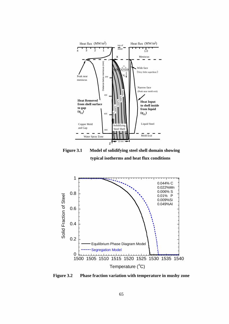
65

Heat fluxHeat flux

Peak nearmeniscus

Copper Moldand Gap

Liquid Steel

1.0123

400

200

top ofmold

23 mm

4

0

Mold Exit

600

Heat Inputto shell insidefrom liquid(q )

Water Spray Zone

Meniscus

Narrow face(Peak near mold exit)

SolidifyingSteel Shell800

Wide face(Very little superheat )

int sh

Heat Removedfrom shell surfaceto gap(q )

(MW/m )2 (MW/m )2

∆x

Vc

i

x

z Figure 3.1 Model of solidifying steel shell domain showing

typical isotherms and heat flux conditions

0

0.2

0.4

0.6

0.8

1

1500 1505 1510 1515 1520 1525 1530 1535 1540

Equilibrium Phase Diagram ModelSegregation Model

Sol

id F

ract

ion

of S

teel

Temperature (oC)

0.044% C0.022%Mn0.006% S0.01% P0.009%Si0.049%Al

Figure 3.2 Phase fraction variation with temperature in mushy zone

66

15

20

25

30

35

40

45

50

55

600 800 1000 1200 1400 1600 1800

AISI 1008

AISI 1026

AISI 1086

1.2%C Carbon Steel

AISI 304

AISI 430

Ther

mal

Con

dutiv

ity (W

/mK

)

Temperature (K)

Lines: Used in CON1DSymbols: Mesaured Data

Figure 3.3 Comparison of model thermal conductivities and measurements[162]

1

10

800 1000 1200 1400 1600 1800

Micro Segregation ModelMeasured Data

Spec

ific

Hea

t (kJ

/kgK

)

Temperature (K)

Material: AISI 1026 steel

Figure 3.4 Comparison of model specific heat curve and measurements [162]

67

1000

1100

1200

1300

1400

1500

0 5 10 15 20 25 30

3 Sec.6 Sec.12 Sec.24 Sec.36 Sec.48 Sec.Te

mpe

ratu

re (o C

)

Distance into Shell (mm)

Lines: Analytical SolutionSymbols: CON1D Predictions

(a) Shell temperature distribution

0

5

10

15

20

25

0 10 20 30 40 50

CON1DAnalytical Solution

She

ll Th

ickn

ess

(mm

)

Time (Second)

(b) Shell growth

Figure 3.5 Comparison of CON1D steel solidification model results

and analytical solutions

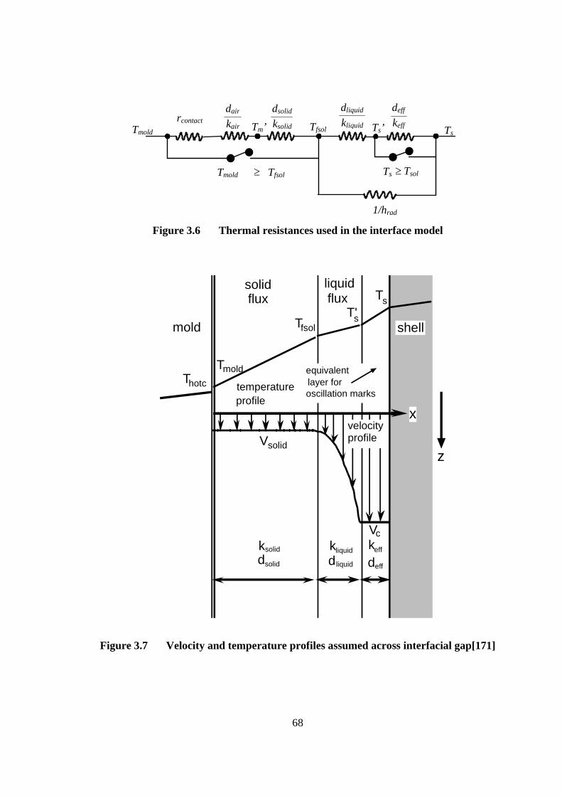
68

Ts

dair

kair

dsolid

ksolid

dliquid

kliquid

deff

keff

1/hrad

Ts Tsol ≥ Tmold Tfsol≥

Tmold rcontact

Tfsol Ts’ Tm’

Figure 3.6 Thermal resistances used in the interface model

mold

liquidflux

V

solidflux

d dd

velocityprofile

T

shell

V

temperatureprofile

equivalentlayer foroscillation marks

k k ksolid

solid

c

fsol

TsT's

moldThotc

solid

liquid

liquid

eff

eff

T

z

x

Figure 3.7 Velocity and temperature profiles assumed across interfacial gap[171]

69

d eff

d mark

Steel Flux

L mark

L pitch d osc

Figure 3.8 Model treatment of oscillation marks[171]

1

10

100

1000

1000 1100 1200 1300 1400 1500

µ1300

=1.1Poise, Tfsol

=1045oC, n=0.85

µ1300

=1.1Poise, Tfsol

=1080oC, n=0.6

Lanyi Flux C2 Measured

Vis

cosi

ty (P

oise

)

Temperature (oC)

Figure 3.9 Comparison of model mold slag viscosity curves and

measurements[100]

70

ferrostatic pressure

molten steel

liquidslag

Vm

elementfor forcebalance

liquid slag pool

steel shellmold

h0

shearstresses

Vc

slag powder

slag rim

top surface meniscus

solidslag

x

z

Figure 3.10 Schematic of interfacial gap in oscillating mold

Mold SolidSlag

LiquidSlag

SteelShell

Maximum Up-stroke

Maximum Down-stroke

Vc

Vm

x

z

Figure 3.11 Schematic profile of slag velocity during oscillation cycle

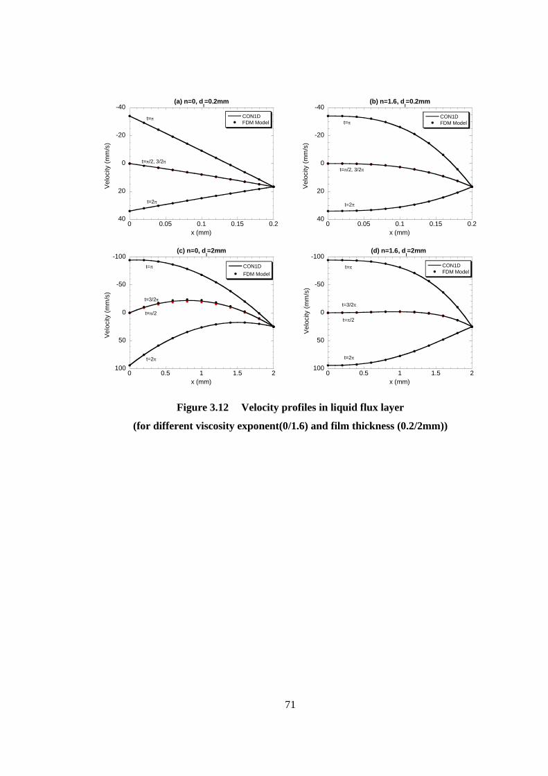
71

-40

-20

0

20

400 0.05 0.1 0.15 0.2

(a) n=0, dl=0.2mm

CON1DFDM Model

Vel

ocity

(mm

/s)

x (mm)

t=2π

t=π/2, 3/2π

t=π

-40

-20

0

20

400 0.05 0.1 0.15 0.2

(b) n=1.6, dl=0.2mm

CON1DFDM Model

Vel

ocity

(mm

/s)

x (mm)

t=π

t=π/2, 3/2π

t=2π

-100

-50

0

50

1000 0.5 1 1.5 2

(c) n=0, dl=2mm

CON1DFDM Model

Vel

ocity

(mm

/s)

x (mm)

t=π

t=3/2π

t=π/2

t=2π

-100

-50

0

50

1000 0.5 1 1.5 2

(d) n=1.6, dl=2mm

CON1DFDM Model

Velo

city

(mm

/s)

x (mm)

t=3/2π

t=π/2

t=π

t=2π

Figure 3.12 Velocity profiles in liquid flux layer

(for different viscosity exponent(0/1.6) and film thickness (0.2/2mm))

72

Up stroke

Down stroke z

x

(a) liquid shear stress limited (b) friction coefficient limited

σz(z)

σz(z+∆z)

τs/l

σx

σx ds

∆z

σz(z)

σz(z+∆z)

τmold

τs/l

σx

σx ds

∆z

σz(z)

σz(z+∆z)

τmax

τs/l

σx

σx ds

∆z

σz(z)

σz(z+∆z)

τmax

τs/l

σx

σx ds

∆z

τmold

Figure 3.13 Force balance on solid slag layer section

(mold wall friction left, liquid layer shear stress right and axial stress)

2mm

Solid SlagLayer

MoldSide

800mm

Liquid SlagLayer Side

σx

τs/l

Figure 3.14 ANSYS solid slag stress model domain, mesh and BCs

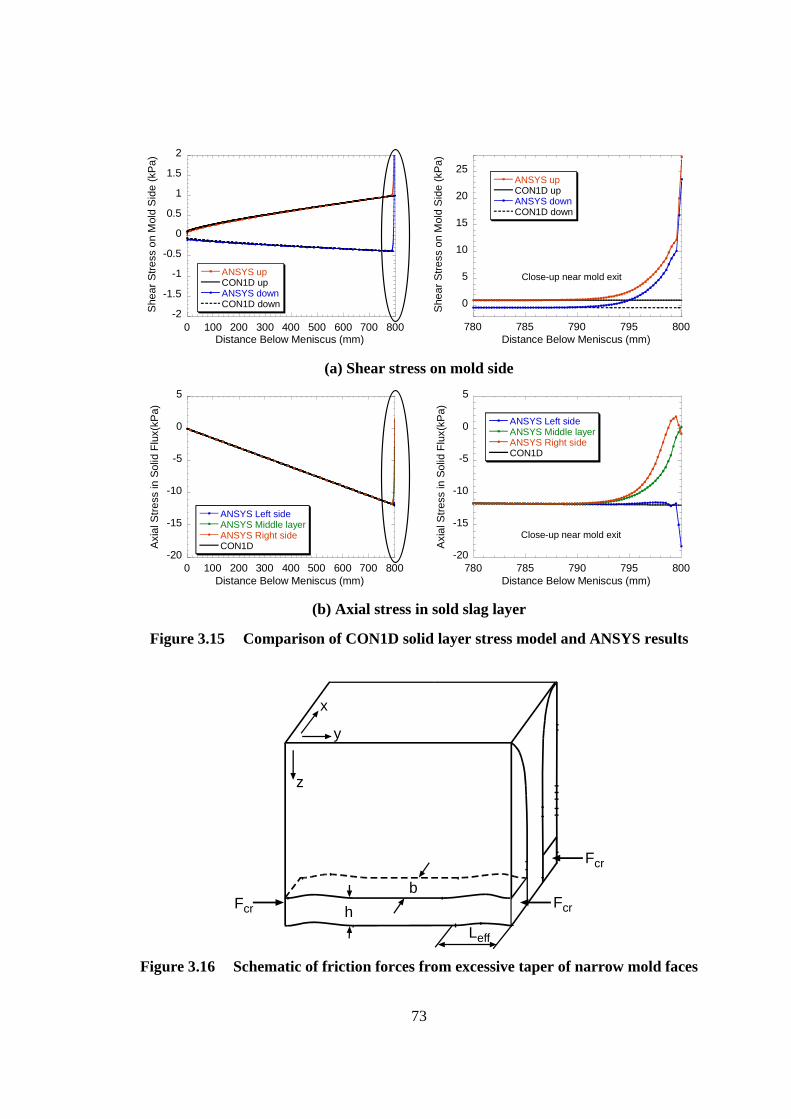
73

-2

-1.5

-1

-0.5

0

0.5

1

1.5

2

0 100 200 300 400 500 600 700 800

ANSYS upCON1D upANSYS downCON1D downS

hear

Stre

ss o

n M

old

Sid

e (k

Pa)

Distance Below Meniscus (mm)

0

5

10

15

20

25

780 785 790 795 800

ANSYS upCON1D upANSYS downCON1D down

She

ar S

tress

on

Mol

d S

ide

(kPa

)


Close-up near mold exit

(a) Shear stress on mold side

-20

-15

-10

-5

0

5

0 100 200 300 400 500 600 700 800

ANSYS Left sideANSYS Middle layerANSYS Right sideCON1DA

xial

Stre

ss in

Sol

id F

lux(

kPa)


-20

-15

-10

-5

0

5

780 785 790 795 800

ANSYS Left sideANSYS Middle layerANSYS Right sideCON1D

Axi

al S

tress

in S

olid

Flu

x(kP

a)


Close-up near mold exit

(b) Axial stress in sold slag layer

Figure 3.15 Comparison of CON1D solid layer stress model and ANSYS results

b

z

y

x

FcrFcr hLeff

Fcr

Figure 3.16 Schematic of friction forces from excessive taper of narrow mold faces

74

CoatingLayers

Tcold Thotc Tmold

dch dmold

Water Channel

2D model zonez

Copper Mold

1D model zone

hwaterTwater

x

qint

meniscus

Zmold

Z2D

Zmen

(a) Vertical section along casting direction

Mold Coating

Fin Copper Mold

Bolt Tcold Thotc Tmold

Twater

wch

Lch

dch dmoldx

y

Water Channel

(b) Horizontal section through mold

Figure 3.17 Simulation domain in mold

75

Moldmold exit=start of Zone 1

Zone 11

2

2

3

start of Zone 3

Zone 2

Zone 3

start of Zone 2

Water Spray

Support Roll

Steel Shell

(a) Typical spray zone configuration

Slab

Roll

Spraynozzle

heat transfer

roll contact, hroll

spray impinging, hspray

natural/forced convection, hconv

radiation, hrad_spray

(b) Heat transfer between one pair of rolls

Figure 3.18 Schematic of spray zone region

76

Initialization: qsh~z, fs~TTmold=Twater,Tsteel=Tpour

Beginning

Heat and mass balance dliquid, dsolid

Calculate heat flux: qint

1D Tmold, Tsteel

2D Tmold

1D Tmold=2D Tmold

Yes

Calculate gaptemperature, friction

Output: End

No

Figure 3.19 Flow chart of CON1D program

77

CHAPTER 4. SLAG PROPERTY MEASUREMENTS AND CHARACTERIZATION

The previous chapter described the mathematical model CON1D. It was shown

that by supplying the model with accurate information, extensive insight can be gained

into steel product behavior and potential quality concerns. Most of the parameters, such

as casting conditions and mold geometry, can be directly obtained from the operating

caster of interest. The heat transfer and lubrication in the interfacial gap depends mainly

on the properties of the slag filling the gap. These properties include chemical

composition, viscosity, friction coefficient and crystallization behavior. Because some of

these properties have not been recorded in previous work, an experimental investigation

was undertaken to gain better understanding of these important mold slag properties.

4.1 Chemical Composition

In this study, four different mold powder or slag-layer-film samples taken during

tail-out were investigated. These four slags are S1 and K1 crystalline slags, S2 glassy

slag, and H1 tail-out film. The chemical compositions of the four slag powder are listed

in Table 4.1, which have been re-calculated from the original suppliers report (Appendix

G[181-183]) by converting F to CaF2. It must be noted that the carbon is added to slow

down the mold powder melting and thereby control melting uniformity during the casting

process. This carbon burns out during the powder sintering and melting process, so is not

generally present in the liquid slag layer or in the re-solidified slag film in the gap. The

powder for slag samples S1 and S2 were prepared without adding the carbon in order to

reproduce the actual molten slag in the continuous casting mold without having to

experience the difficulties associating with decarburization.

78

4.2 Friction Coefficient

The modeling work in Chapter 3 shows that the slag properties near the

solidification temperature are very important to interfacial lubrication. However, previous

research focuses only on the properties at high temperature (greater than 1000oC)[99,

101, 130, 135, 136, 151-153, 184], The lubrication properties of flux near the softening

temperature are rarely reported. Thus, laboratory experiments measuring the friction

coefficient of the solid slag layer from room temperature up to 1000oC were conducted.

4.2.1 Sample Preparation and Instrumentation

The prepared relatively carbon free mold powder was melted in a graphite

crucible (with Zr coating) at 1400oC for an hour, and then poured into a preheated metal

dish (Steel/high temperature Ni alloy). The inner diameter of each sample holder is 20-

30mm and the depth is 5mm. The sample surface was polished using 120~600 grit coarse

sand paper to get a flat surface with roughness Ra about 0.2µm~0.6µm, as measured

using a Dektak 3030 profilometer at the Center for Microanalysis of Materials (CMM) at

UIUC. Each sample was then tested with a High Temperature Tribometer (HTT) at the

Tribology and Micro-Tribology Lab at Department of MIE, UIUC, shown in Figure 4.1.

The HTT can measure detailed friction and wear data on material test specimens

up to 1000oC. It consists of a rotating/oscillating spindle on which the plate specimen is

mounted and a special holder applies the contact load through a pin while measuring both

the normal and friction forces. The pin, holder and sample are contained within a

cylindrical furnace that features spiral heat coils and is insulated with special reflective

film to encourage uniform radiative heating in the interior. The entire unit is enclosed in a

79

sealed bell jar. Vertical movement of the specimen into and out of the furnace and precise

control of the movement to regulate the pin loading are provided by a remotely operated

drive system[185].

4.2.2 Experimental Procedure

The pin is a 0.25inch diameter steel ball bearing except for run #A, which used a

ring shaped pin with a flat surface(Do/Di=1”/0.25”). The wear track diameter is set to

0.375inch except for Run #8. The spindle velocity is varied from 50rpm to 300rpm,

which corresponds to speeds of 25mm/sec to 150mm/sec. For run #8, the track diameter

is 0.715inch. To keep same velocity range, the rotating frequency is adjusted to

26~158rpm correspondingly.

The first series of experiments began from room temperature and increased every

100oC until the machine limit (~900oC). It took 3~5 minutes for temperature to reach

each set point, which was increased in 100oC intervals. After waiting 5 minutes, data was

recorded from the display every two seconds for two minutes, giving 60 data points for

each state.

To investigate reproducibility and the importance of time in the apparatus, the

second series of experiments was conducted by heating to the highest temperature in only

40 minutes and recording data during decreasing temperature intervals using the above

recording procedure. Wear track depths were measured with a profilometer which is able

to quantify depth from 0.02mm to 25mm[186].

80

4.2.3 Results and Discussion

Table 4.2 gives the temperature process of each different run and the

corresponding maximum wear track depth. The machine was calibrated after run #2.

Comparing the HTT LCD displayed friction coefficient and the real friction coefficient

during calibration using known weights applied tangentially and normally, Figure 4.2

shows the deviation is in a reasonable measurement error range. However, runs #A and

#1 were conducted before machine calibration, so we can only rely on the tendency of the

friction coefficient as the values appear to be too large.

Figure 4.3(a) shows a sample of data recorded for slag S1 in run #5 at 400oC. The

variation is different for different conditions. Figure 4.3(b) plots the average friction

coefficient for 25mm/s velocity, with the variation range at every temperature shown as

error bars. Higher velocity slightly increases the friction coefficient, but this effect is

negligible for temperatures above 500oC, as shown in Figure 4.3(c).

Figure 4.4 gives the results of four runs for slag S1. The direction of the arrow on

each line shows evolution of temperature during heating or cooling. The value of the

friction coefficient varies between runs with average value 0.16 ± 0.1 excluding run #1.

Increasing temperature above 800oC causes the friction coefficient to begin to drop. This

decrease might correspond to the oxidation layer formed on the top steel ball bearing pin

or alternatively to material softening. In general, there seems to be a slight trend of

decreasing friction with increasing temperature which is consistent with a softening

phenomenon. However there is lots of variation that can be explained by oxidation. An

oxide layer is believed to lubricate the metal/slag interface[187]. Thus, run #7 shows a

hysteresis loop with lower friction at later time at the same temperature due to oxide layer

81

build-up. The increase of friction just after starting to decrease temperature at the

beginning of runs #5 and #8 might be due to spalling of the oxide. Figure 4.5 shows

pictures of the specimens after the friction tests. Two different friction mechanisms seem

to have affected these two runs. Run #1 shows adhesive friction while run #5 is more

likely to be abrasive friction. The measurement of wear track depth shows that run #5 has

much deeper wear than run #1 (152µm vs. 24µm), which is consistent with the two

proposed mechanisms.

Figure 4.6 shows the friction coefficient as a function of temperature for slag S2

based on runs #3, #4 and #6. It appears that the friction has a slight drop from room

temperature to 500oC. Just above 500oC, the friction coefficient increases sharply from

0.1 to 0.5. This is because the specimen begins to soften. Instead of wear, the ball bearing

plows through the tacky slag layer and causes an artificially high increase of friction

coefficient. Figure 4.7 shows pictures of slag S1 before and after the test. It confirms that

the sample got soft and deformed greatly during the experiment. With increasing

temperature, the specimen became too soft to withstand any normal force. After this

softening and accompanying deformation, decreasing temperature caused the friction

coefficient to fluctuate between 0 and 1.5. This indicates that the surface was too rugged

to make any effective measurement, which also happened to a specimen where open

bubble holes appeared in the wear track. For the test with slag K1, a similar friction

increase with material softening was observed at 720oC as shown in Figure 4.8. The more

gradual increase for this test might be due to the use of a different top pin with a flat

surface.

82

The results show that the friction is relatively insensitive to the microstructure of

the slag. It generally stays below 0.2 before softening. The softening of the slag, indicated

by the apparent dramatic increase in friction coefficient occurs at much lower

temperature than previously supposed. This work, for the first time, enables a way to

extend the viscosity curves to a lower temperature range.

4.3 Viscosity

Viscosity and solidification temperature have been identified as the key physical

properties in selecting a powder with suitable heat transfer properties[5]. Together with

the chemical composition, Powder manufacturers commonly measure viscosity at high

temperature, as shown in Figure 4.9. Only the low viscosity part of the curve(<400poise)

can be measured with a viscometer. Note that the viscosity of slag H1 was fitted from

measurements using Eq.(3.19) with µ1300=3.1poise, Tfsol=1130oC and n=1.682[183].

From the high temperature friction test, we know that slags S2 and K1 soften at

500oC and about 720oC, and that slag S1 will likely begin to soften at 1000oC or above.

For slag S2, the normal force dropped from 10N to 7N in about one minute while the

wear check depression grew to 0.5mm deep. The magnitude of the slag viscosity at the

softening point can be estimated roughly from its definition assuming Newtonian flow:

z

z

θ

θ

τµγ

= (4.1)

The shear stress, zθτ can be estimated from the recorded friction force, F, and the contact

area, A:

63.0 30 103.14 3.175 0.01z

F F N PaA rh mm mmθτ

π= = = ≈ ×

× × (4.2)

83

Where, r is the radius of the ball bearing, h is the increase in depression depth over one

revolution. The strain rate, zθγ can be estimated by assuming 0zvθ

∂=

∂:

11 25 / sec 5sec5

zz

v v vv mmz r z z mmθ θ θ

θγθ

−∂ ∂ ∆∂= + = ≈ ≈ =

∂ ∂ ∂ ∆ (4.3)

Where, ∆z is the slag layer total thickness, vθ is the rotation speed. Combining equations

(4.1)-(4.3) gives a viscosity of about 76 10 Poise× . This value matches with the viscosity

of common glass at its softening point shown in Figure 2.5[126]. Thus, we can extend the

viscosity curves to the low temperature-high viscosity (108poise) region, as shown in

Figure 4.9. This figure also shows the CON1D model fit through the data points using

Eq.(3.19). It is interesting to note that the measurements show inflection(s) occur in the

high temperature portion of each curve perhaps due to partial crystallization. The data for

slag K1 and this work both show that the inflections are just a minor fluctuation in the

entire curve. The CON1D model fitting equation does not capture this effect.

4.4 Crystallization Study

It is well known that the proportion of crystalline and glassy phases in the slag

film is important to the control of heat transfer in the mold[139, 140, 188] A thicker

crystalline layer decreases heat transfer and is helpful to reduce surface defects for

peritectic steels[189, 190]. However, slag with a high crystallization tendency is also

reported to increase the friction between the mold and the strand which might cause

sticking type breakouts[69, 191]. A series of experiments were conducted to study the

crystallization behavior of slags S1 and S2.

84

4.4.1 Experimental Methods

The onset of crystallization is a strong function of cooling rate in slags because

they do not crystallize easily. Three methods were used to investigate time temperature

transformation phenomena in slags S1 and S2 over a wide cooling rate range.

A. Differential Scanning Calorimetry (DSC) (CCT tests)

DSC is a common technique used to determine phase transformations at slow

cooling rate. The test material is subjected to a controlled temperature program by online

feedback control of the heat input simultaneously with a reference substance that

experiences no phase transformation over the temperature range of interest. The

difference of heat flow between the two samples is recorded. The signal is then corrected

by subtracting the heat flow difference signal obtained from a calibration (baseline) run

using two identical reference samples. Deviations in the heating or cooling rate are

attributed to phase transformations in the test sample. An endothermic phase

transformation causes a dip in the heating rate curve during a heating test. During a

cooling test, the reverse phase transformation is exothermic, causing a peak spike in the

cooling rate curve. The onset temperature of the exothermic peak is an indicator of a

crystallization reaction. In a slag with only one peak, this is often called the

“Crystallization Temperature” of the mold slag[143].

The DSC experiments were conducted on a Netzsch STA 409 at the Center for

Cement Composite Materials (CCM), UIUC, which is capable of both gravimetric (TG)

and thermal analysis simultaneously. The temperature range for TG/DSC is -100 to

1600oC.

85

Slags S1 and S2 were analyzed by TG/DSC. 60~80mg of decarbonized mold

powder was poured into a platinum micro-crucible. Pure alumina (Al2O3) was selected as

the reference for all tests conducted. The temperature was increased from room

temperature to 1300oC for slag S1 and 1100oC for slag S2 at a heating rate of 10oC/min.

These temperatures were sufficient to fully melt each powder. Each sample was then

cooled to room temperature at cooling rates of 1oC/min, 5oC/min and 30oC/min in

separate tests. The heat flow vs. temperature/time curve was recorded and corrected with

the reference baseline run.

B. Dip thermocouples (CCT Tests)

To investigate intermediate cooling rates, a series of thermocouple dip tests were

conducted at the Advanced Materials and Processing Laboratory (AMPL), University of

Alberta, Canada. In these tests, a thermocouple is dipped into the slag melt in a Zr coated

graphite crucible. It takes a few seconds for the thermocouple to heat up to the slag

temperature and reach thermal equilibrium. Then the thermocouple is withdrawn into the

air, with a droplet of the slag stuck around the thermocouple bead. The temperature of the

thermocouple is continuously recorded by the data acquisition system using InstruNet

v2.0. By adjusting the initial melt temperature, or by exposing the dip around the

thermocouple to different atmospheric conditions, such as forced convection, a range of

cooling rates, 0.5°C/sec~50°C/sec, could be achieved. Table 4.3 lists the cooling rate

ranges of different dip thermocouple tests.

C. Atomization (Glass formation)

The real continuous casting process involves rapid initial quenching of the liquid

slag against the mold wall followed by slower cooling at different temperatures according

86

to position in the slag layer (see Figure 6.3). To reproduce the high cooling rates, an

Impulse Atomization Process (IAP) was used. The IAP is a single fluid atomization

technique capable of producing droplets of a predictable mean particle size and a

relatively tight standard deviation under controlled atmospheric conditions, which is

available at the AMPL, Alberta Canada[192]. Here the mold powder was placed in a

graphite crucible and heated in an enclosed tower in a nitrogen atmosphere. At the

bottom of the crucible, an array of orifices was machined. By vibrating a plunger inserted

into the melt, the molten slag is forced out of the orifices at the bottom of the crucible.

The streams are disintegrated into droplets and fall through the chamber. A mathematical

model of droplet solidification which was developed by researchers in the AMPL was

used to predict the cooling history of the droplets[193]. By varying the atomization

parameters, particle cooling rates due to the radiation and convection were obtained

ranging from 100°C/sec to 13000°C/sec depending on particle size. Figure 4.10 shows

the schematic of the Impulse Atomization Process[192].

D. Furnace holding (Devitrification tests)

The atomized material was confirmed to be in a fully glassy state through XRD

measurements (described in the next section). This material was then subjected to

reheating and furnace holding to investigate devitrification. The amorphous particles

were put into a preheated furnace maintained at different temperatures (500oC to

1100oC). After the sample had been held for a set time as shown in Table 4.4, it was

taken out, water quenched to room temperature and analyzed with XRD.

87

4.4.2 X-ray Diffraction (XRD)

The treated samples were submitted for XRD analysis to examine the phases

present in order to investigate the evolution of crystallization. This study used a Rigaku

Geigerflex Powder Diffractometer with a Co tube (Kα1 λ=1.78897Å) and a graphite

monochromator to filter the Kβ wavelength at the Department of Earth & Atmospheric

Sciences, University of Alberta, Canada with operation conditions of 40kV and 30mA,

and the Rigaku D-Max X-ray diffractometer using Cu radiation (Kα1 λ=1.54056Å) at the

CCM, UIUC with operation conditions of 40kV and 20mA. At the CCM, each XRD

spectrum was collected between 5o and 70o 2θ angle. A step size of 0.02o was used at a

scanning speed of 1.2o/min. The collected data were analyzed using analytical software,

Jade6.5. The XRD results using different radiation sources were converted with the

following relation:

( )( )

sinsin

θ λθ λ

=Cu Cu

Co Co

(4.4)

After this conversion, the results for the same specimen from the different X-ray

diffractometers matched very well.

4.4.3 Results and Discussion

A. DSC curves

Figure 4.11 shows the DSC curves for slags S1 and S2 generated at a constant

heating rate of 10oC/min and different cooling rates of 1oC/min, 5oC/min or 30oC/min.

The sharp endothermic trough of the heating curves at 100oC is due to water evaporation.

Figure 4.11(a) also show two endothermic troughs occurred around 450oC and 750oC,

88

which are associated with the decomposition of carbonates. The carbonates normally

used in casting powders are CaCO3, and Na2CO3. The 450oC endotherm might be due to

the decomposition of Na2CO3 and the 750oC endotherm is probably related to the

decomposition of CaCO3[194]. This is confirmed by the accompanying weight loss

included in Figure 4.11(a) (TG), which is expected because of the volatization of CO2.

The series of endothermic peaks above 1000oC on the heating curve indicates that the

powder began to melt incongruently. The end of the last peak encountered on heating

presumably represents the liquidus temperature. This is seen to be 1235oC for slag S1.

During the cooling process, the phase transformations are very different from

heating, owing to the irreversible chemical reactions that occur during melting. Several

exothermic peaks were observed, where again phase transformations are indicated. On

cooling, the phase transformation is believed to begin at the inflection point starting each

peak. For slag S1 at 1oC/min cooling rate, shown in Figure 4.11(a), the exothermic peaks

begin at 1234oC, 1160oC and 1022oC, which might correspond to the onset of three

different crystalline phases forming.

In general, a higher cooling rate increases the peak height, whereas a lower rate

yields higher resolution[195]. Higher cooling rates delay both the onset and finish of each

phase transformation. The corresponding temperatures are also labeled in Figure 4.11(a).

Similar analysis is conducted for slag S2. The results show a lower liquidus

temperature of 1050oC and different exothermic peaks during cooling, as labeled in

Figure 4.11(b). The information in Figure 4.11 is presented later to construct continuous

cooling transformation curves.

89

B. Thermocouple dip tests cooling curves

The cooling curves recorded during the thermocouple dip tests were smoothed

using the Savitzky-Golay polynomial smoothing filter to eliminate noise[167]. The

Savitzky-Golay algorithm is based on performing a least squares linear regression fit of a

polynomial of degree K over at least K+1 data points around each point to smooth the

data. The filter coefficients: the order of the polynomial, K, the number of passes, P and

the frame size, F are taken to be 2, 3, 9. These values are chosen to preserve higher

moments in the data, thus reducing the distortion of essential features of the data such as

peak heights and line widths in the spectrum, while efficiently suppressing random noise

that degrades derivative calculation. Figure 4.12(a) compares the recorded thermocouple

temperature and the filtered curve.

The temperature history curves were numerically differentiated with second order

accuracy to distinguish points where the thermal gradient changes would be indicative of

crystallization. As an example, Figure 4.12(b) shows two points marking the onset of

sharp drop in cooling rate where the beginning of crystallization is believed to occur for

slag S1 test K. Figure 4.12(c), (d) show temperature gradient profiles of thermocouple dip

tests for both slags with labeled points of interest. These points were used for

constructing CCT curves.

C. X-Ray diffraction results

XRD was carried out for the initial decarbonized slag powder, re-solidified

atomization particles and samples after thermocouple dip tests and furnace holding tests.

Figure 4.13 displays the intensity distribution as a function of diffraction angle of the slag

powders before melting, and indicates that the six main phases are: silica (SiO2), calcium

90

fluoride (CaF2), wollastonite (CaSiO3), calcite (CaCO3), calcium silicate (Ca3SiO5) and

sodium carbonate (Na2CO3).

The crystalline phases identified in the thermocouple dip tests and furnace

holding devitrification tests are summarized in Table 4.5 and Table 4.6. The atomized

particles had no peaks for crystalline phases, indicating that all droplets of both slags

were completely amorphous. The peaks are weaker relative to the background noise for

all samples, compared with the slag powder, indicating that the melting and re-

solidification produced some glass in every test. Cuspidine (3CaO•2SiO2•CaF2 or

Ca4Si2O7F2) is identified in all non-amorphous specimens. The thermocouple dip tests for

slag S1 with slower cooling rates (Test D, K, I) indicate calcium silicon oxide fluoride

(SiO2•2CaF2 or Ca2SiO2F4)[196] phase also, as shown in Figure 4.14. This shows that

cuspidine crystallizes easily and that perhaps Ca2SiO2F4 crystallization is suppressed by

the higher cooling rate.

Figure 4.15 indicates the evolution of crystalline phase(/s) forming at

progressively longer holding times in the furnace devitrification tests from the glassy

state at 700oC. In slag S1, the first (easiest) phase to form is cuspidine which first appears

after holding at 700oC for 30 minutes. With increasing furnace temperature, different

phases are found as shown in Figure 4.16. Nepheline (Na2O•Al2O3•2SiO2 or NaAlSiO4)

is found in slag S1 at temperatures greater than 900oC. Holding slag S1 longer than one

hour at 1100oC causes the peaks of nepheline to disappear and a new phase, gehlenite

(2CaO•2Al2O3•SiO2 or Ca2Al2SiO7) to form, as shown in Figure 4.16(a). This

phenomenon was also observed by Grieveson[197] and O’malley[198].

91

For slag S2, no crystalline phase forms at 500oC even after two hours of holding.

Besides cuspidine, some new phases such as nepheline and calcium silicate (2CaO•SiO2

or Ca2SiO3, 8CaO•5SiO2 or Ca8Si5O18) are found in slag S2 when holding at 700oC for

two hours. Instead of gehlenite in slag S1, a sodium calcium silicate phase

(Na2O•2CaO•3SiO2 or Na2Ca2(SiO3)3) is found at 900oC. When the holding temperature

is near to the slag melting temperature, only a small amount of crystalline cuspidine

phase is observed in the amorphous background(Figure 4.16(b)). This might due to the

lower driving force for crystallization at higher temperature.

D. CCT curves

From the time-temperature profiles recorded during the DSC tests and

thermocouple dip tests, CCT diagrams were constructed by taking time starting at zero

when the cooling curves crossed the liquidus temperature (1235oC for slag S1 and

1050oC for slag S2). Figure 4.17(a) shows the CCT diagram for slag S1. The critical

cooling rate to maintain the amorphous structure is estimated to be 50oC/s. At slower

cooling rate, the first crystalline phase appears at around 1200oC, which should be

cuspidine (Ca4Si2O7F2) according to the XRD analysis. Watanabe measured that the

liquidus of cuspidine varies between 1114oC (55% CaF2) and 1407oC (20% CaF2) in the

CaO-SiO2-CaF2 ternary system(Figure 2.4(a))[123]. For the slag S1, Figure 2.4(a) shows

a liquidus temperature of 1250oC, which almost matches with the result in this work. As

slag S2, the liquidus temperature is found to be lower. This might be due to the effect of

many other compounds in the slag, especially Na2O, Al2O3 etc, which decrease the

system melting temperature. When the cooling rate is slower than 10oC/s, a second

crystalline phase is formed at around 1100oC, which could be silicon oxide fluoride

92

(Ca2SiO2F4) phase. The DSC tests with very slow cooling rate (<5oC/min) shows a third

peak near 900oC as shown in Figure 4.11(a), implying the existence of a third phase,

which could not be distinguished in the XRD pattern of the thermocouple dip tests. The

cooling curves of the dip tests are more ambiguous but do not appear to show the third

phase either. This suggests that this phase is suppressed at the faster cooling rate in

comparison to the DSC tests. The XRD results from furnace heating devitrification tests

confirm that more crystalline phases form at 900oC to 1100oC. Comparing these results

with the phase diagrams in Figure 2.4, these phases generally shows lower liquidus line

which is due to the eutectic reaction between each other.

Similarly, Figure 4.17(b) shows the CCT diagram for slag S2 featuring a critical

cooling rate of only 20oC/sec. This low critical cooling rate confirms the conjecture that

slag S2 is glassy. The cuspidine (Ca4Si2O7F2) phase starts to form at around 1050oC.

Other crystalline phases were observed from isothermal aging tests as described in

previous section, though they are difficult to be distinguished unambiguously in the XRD

pattern and cooling curves of thermocouple dip tests.

4.5 Slag Film Microscopy

4.5.1 Polarized Transmitted Light Microscopy

Polarized Light Microscopy is a technique that examines a material's optical

properties to investigate its microstructure. It can be best applied to materials that are

anisotropic and have two indices of refraction. These materials are called "birefringent".

When polarized light enters a birefringent material, it splits up into two rays that vibrate

along the two principal directions of the anisotropic crystal lattice. One of these rays is

called the fast ray, and the other the slow ray. By the time the rays emerge from the

93

specimen, one of them has been retarded, or slowed down, more than the other and this

angle of retardation can be used to deduce the crystal structure of the material[199].

Specifically, retardation measurements are typically applied to distinguish between

isotropic and anisotropic materials.

Isotropic materials, which include gases, liquids, and glasses, demonstrate the

same optical properties in all directions. They have only one refractive index and no

restriction on the vibration direction of light passing through them. Thus when the

isotropic specimen is examined under cross polarized light, no retardation of either ray

occurs, so total extinction of the reassembled light is observed. Anisotropic materials, in

contrast, have optical properties that vary with the orientation of incident light with the

crystallographic axes. They demonstrate a range of refractive indices depending both on

the propagation direction of light through the substance and on the vibrational plane

coordinates. More importantly, anisotropic materials act as beam splitters and divide light

rays into two parts. The technique of polarizing microscopy exploits the interference of

the split light rays, as they are re-united along the same optical path to extract structure

information about these materials.

A piece of film of slag H1 from interfacial steel shell/mold gap was caught as it

folded off the mold wall during tail-out after continuous casting process[200]. The slag

film was cut into thin slices only 0.03mm thick and mounted on microscope slides, which

are called “thin sections”. The thin section specimen was then observed under polarized

light microscopy, which was carried out at the Department of Geology, UIUC.

Figure 4.18(a) shows the different layers and cracks in the slag film under plane

polarized light. Figure 4.18(b) to (d) are the images under cross polarized light obtained

94

by rotating the specimen stage. The extinction on the steel side layer proves that it is

isotropic. Because crystals of any size or composition have some anisotropic properties,

this indicates that the layer is a glassy layer. This suggests that the layer was formed from

air quenching the liquid slag while obtaining the sample. Note that the critical cooling

rate for obtaining glass is well below typical cooling rates encountered during air cooling,

so this finding is reasonable. (Lumped parameter cooling analysis with slag layer

thickness of 2mm, heat transfer coefficient of 200W/m2K and conductivity of 1.5W/mK

produce the Biot number of 0.26 and a cooling rate of 80oC/sec)

4.5.2 Scanning Electron Microscopy (SEM)

To further investigate the morphology and composition distribution of the slag

film, an SEM microstructure analysis was carried out on the Zeiss DSM 960 with an

energy dispersive x-ray spectroscopy system (EDX), which is available at the Center for

Microanalysis of Materials (CMM) at UIUC. It has a LaB6 source to provide a stable

beam for quantitative analysis and is also equipped with a system for the observation of

backscattering patterns.

Figure 4.19(a) shows the backscatter electron image (BSE) of the slag H1 film.

Figure 4.19(b) is a close-up of the interface between the two layers. Crystals on the left

can be clearly seen growing into the glassy layer on the right. To investigate the

composition distribution in the specimen, a series of EDX mapping was performed. Each

image was created by mapping the X-ray intensity at each point for a specific element. As

shown in Figure 4.20, the bright region indicates where the specific element has a high

concentration. On the right side of each image, all elements are distributed

homogenously, which again confirms the glassy microstructure of the right side. The

95

EDX spectrum was also used to identify the element composition of different regions in

the sample. The crystalline side (left) is composed of high-calcium grains (point B) in a

high-silicon background (Point D). These likely represent crystals of cuspidine that

precipitated. Figure 4.21(a)-(c) indicate that the area average composition is almost the

same for the crystal and glassy regions, which indicates that no severe macro-segregation

occurred in the gap during casting.


Table 4.1 Mold Powder Composition (wt%)

S1 S2 K1 H1

SiO2 34.33 38.33 31.38 36.01

CaO 29.69 13.30 21.52 35.74

Al2O3 5.55 2.43 4.85 4.63

CaF2 15.93 14.05 28.12 6.82

Na2O 4.75 13.44 9.57 6.04

MgO 3.05 1.45 0.84 <3.0

TiO2 <1.0 <0.5 - <3.0

Fe2O3 <1.5 <1.5 0.20 <3.0

MnO <1.0 <0.5 0.01 <3.0

K2O <1.0 <0.5 0.80 <3.0

Li2O - <1.0 - -

B2O3 - 1.41 - -

C-Total 4.11 11.49 2.36 5.73

CO2 3.22 3.78 2.75 -

C-Free 3.23 10.46 1.61

96

Table 4.2 HTT Friction Tests

Test # Slag Process Maximum wear track depth (µm)

Run #A K1 Increase Temperature from 25oC to 870oC - (softened)

Run #1 S1 Increase Temperature from 25oC to 980oC 24

Run #5 S1 Decrease temperature from 920oC to 80oC 152

Run #7 S1 Increase Temperature from 25oC to 900oC,

then decrease temperature from 900oC to 200oC 249

Run #8 S1 Decrease temperature from 890oC to 200oC 102

Run #3 S2 Increase Temperature from 25oC to 300oC -

Run #4 S2 Increase Temperature from 25oC to 550oC 2254 (softened)

Run #6 S2 Increase Temperature from 25oC to 550oC 1460 (softened)

Table 4.3 Dip Thermocouple Tests Cooling Rates Range (oC/sec)

Slag S1 Test F Test E Test D Test K Test I

CR range 22~40 20~50 10~16 0.7~20 1.1~15

Slag S2 Test 1 Test 2 Test 9

CR range 1.3~20 0.7~15 0.5~6

Table 4.4 Slag Annealing Treatment

1min 10min 30min 60min 120min

500oC S2 S2 S2 S2

700oC S1, S2 S1, S2 S1 S1, S2

900oC S1, S2 S1, S2 S1, S2 S1, S2 S1, S2

1000oC S2

1100oC S1 S1 S1 S1

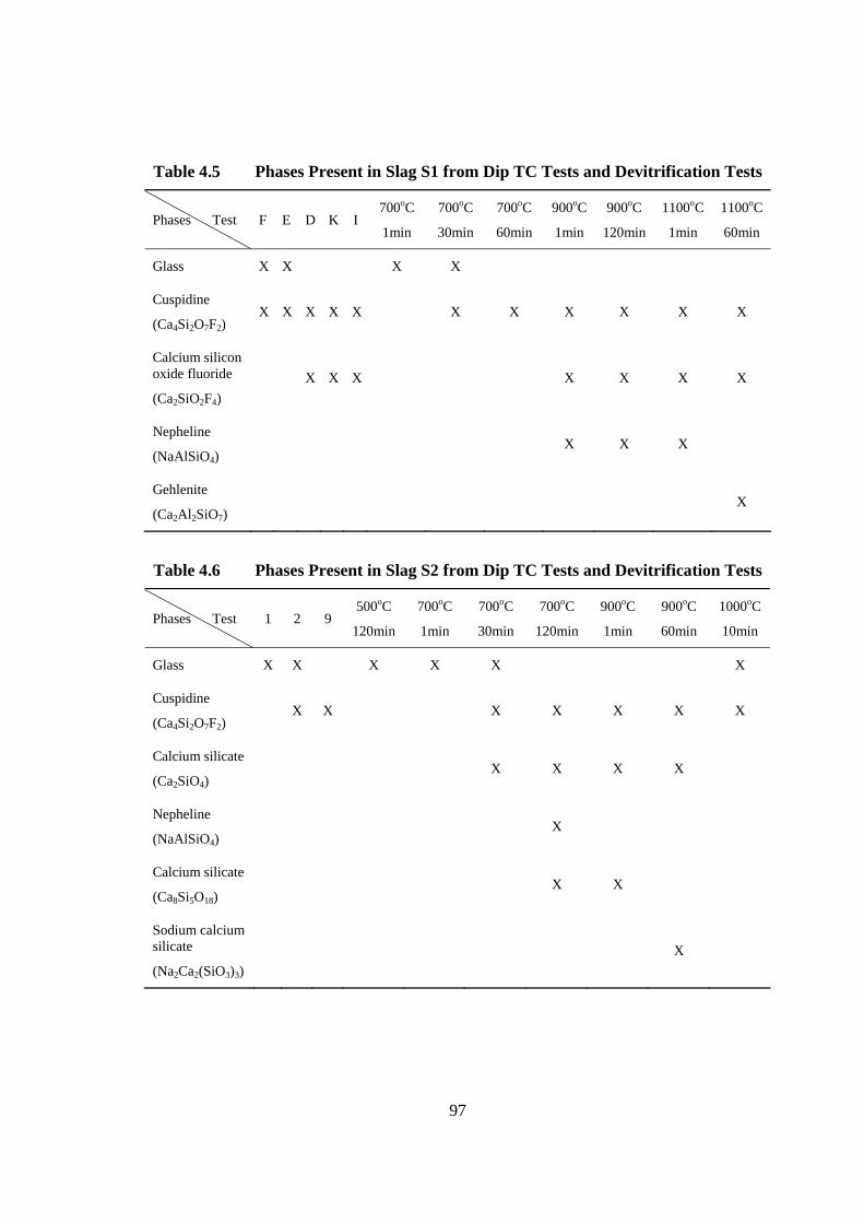
97

Table 4.5 Phases Present in Slag S1 from Dip TC Tests and Devitrification Tests

Phases Test F E D K I 700oC

1min

700oC

30min

700oC

60min

900oC

1min

900oC

120min

1100oC

1min

1100oC

60min

Glass X X X X

Cuspidine

(Ca4Si2O7F2) X X X X X X X X X X X

Calcium silicon oxide fluoride

(Ca2SiO2F4) X X X X X X X

Nepheline

(NaAlSiO4) X X X

Gehlenite

(Ca2Al2SiO7) X

Table 4.6 Phases Present in Slag S2 from Dip TC Tests and Devitrification Tests

Phases Test 1 2 9 500oC

120min

700oC

1min

700oC

30min

700oC

120min

900oC

1min

900oC

60min

1000oC

10min

Glass X X X X X X

Cuspidine

(Ca4Si2O7F2) X X X X X X X

Calcium silicate

(Ca2SiO4) X X X X

Nepheline

(NaAlSiO4) X

Calcium silicate

(Ca8Si5O18) X X

Sodium calcium silicate

(Na2Ca2(SiO3)3) X

98

Figure 4.1 High Temperature Tribometer

0

0.1

0.2

0.3

0.4

0.5

0 0.1 0.2 0.3 0.4 0.5

Rea

l Fric

tion

Coe

ffici

ent

Displayed Friction Coefficient

Figure 4.2 Comparison of HTT displayed friction

coefficient and real friction coefficient

99

0

0.05

0.1

0.15

0.2

0.25

0.3

0.35

0.4

0 10 20 30 40 50 60

25mm/s

50mm/s

150mm/s

Fric

tion

Coe

ffici

ent

number recorded

Slag S1, Run #5, 400oC

0

0.05

0.1

0.15

0.2

0.25

0.3

0.35

0.4

0 200 400 600 800 1000

Fric

tion

Coe

ffici

ent

Temperature (oC)

Slag S1, Run #5, 50mm/s

(a) Friction variation with time (b) Friction variation with temperature including “error bars” to indicate data ranges

0

0.05

0.1

0.15

0.2

0.25

0.3

0.35

0.4

0 200 400 600 800 1000

50rpm

100rpm

300rpm

Fric

tion

Coe

ffici

ent

Temperature (oC)

Slag S1, Run #5

(c) Average friction coefficient vs. temperature at different speeds

Figure 4.3 Friction coefficient for slag S1 Run #5

0

0.1

0.2

0.3

0.4

0.5

0.6

0 200 400 600 800 1000

Run #1Run #5Run #7Run #8

Fric

tion

Coe

ffici

ent

Temperature (oC)

Slag S1

heating or cooling

velocity: 50mm/sec

Figure 4.4 Friction coefficient vs. temperature for slag S1

100

(a) Run #1 (b) Run #5

Figure 4.5 Picture of the specimen for slag S1 after tests

0

0.1

0.2

0.3

0.4

0.5

0.6

0 100 200 300 400 500 600

25mm/s50mm/s150mm/s

Fric

tion

Coe

ffici

ent

Temperature (oC)

Slag S2

Figure 4.6 Friction coefficient vs. temperature for slag S2 (Runs #3, #4 and #6)

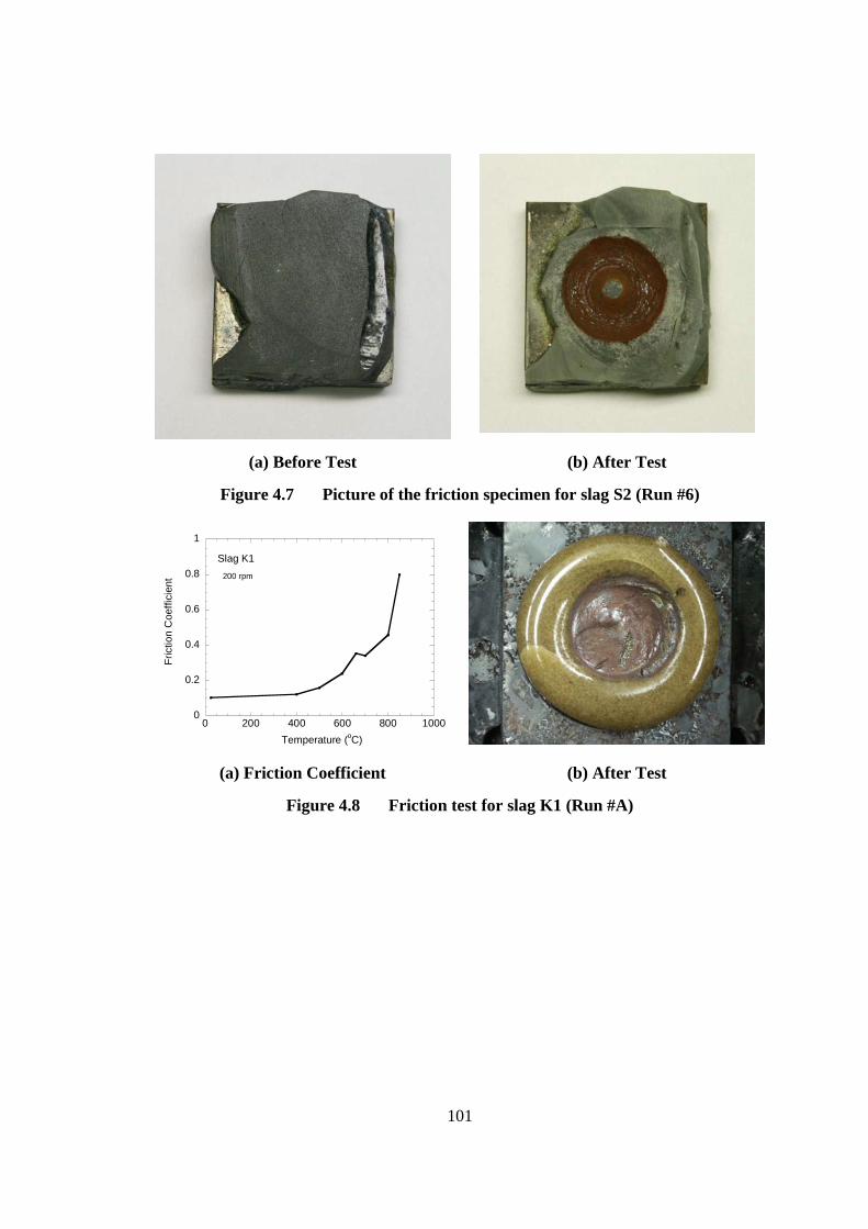
101

(a) Before Test (b) After Test

Figure 4.7 Picture of the friction specimen for slag S2 (Run #6)

0

0.2

0.4

0.6

0.8

1

0 200 400 600 800 1000

Fric

tion

Coe

ffici

ent

Temperature (oC)

200 rpm

Slag K1

(a) Friction Coefficient (b) After Test

Figure 4.8 Friction test for slag K1 (Run #A)

102

1

10

100

1000

104

105

106

107

108

600 800 1000 1200 1400

Slag S1Slag S2Slag K1

CON1D: µ1300

=2.54Poise, Tfsol

=990oC, n=4.5

CON1D: µ1300

=1.12Poise, Tfsol

=425oC, n=7.5

CON1D: µ1300

=0.421Poise, Tfsol

=650oC, n=8.5

Slag H1 (fitted: 1300=3.1Poise, Tfsol

=1130oC, n=1.682)

Visc

osity

(Poi

se)

Temperature (oC)

measured

Figure 4.9 Measured slag viscosity with CON1D fitted curves

Figure 4.10 Impulse Atomization Process[192]

103

-2

0

2

4

6

8 -10

-8

-6

-4

-2

0

0 200 400 600 800 1000 1200Temperature (oC)

Tem

pera

ture

Diff

eren

ce (u

V) ex

o

TG (%

)

TG

DSC

: Heating at 10oC/min

: Cooling at 1oC/min

Tmelt

=1235oC

1234oC

1160oC1022oC

-2

0

2

4

6

8

10

12 -7

-6

-5

-4

-3

-2

-1

0

0 200 400 600 800 1000

TG (%

)

Temperature (oC)

Tmelt

=1050oC: Heating at 10oC/min

: Cooling at 1oC/min

1022oC

TG

DSC

Tem

pera

ture

Diff

eren

ce (u

V) ex

o

-5

0

50 200 400 600 800 1000 1200

Temperature (oC)

Tmelt

=1235oC

Heating at 10oC/min

Cooling at 5oC/min943oC

1230oC

1091oC

Tem

pera

ture

Diff

eren

ce (u

V) ex

o

-4

-2

0

2

4

6

80 200 400 600 800 1000

Temperature (oC)

Tmelt

=1050oC

Heating at 10oC/min

Cooling at 5oC/min

733oC 1034oCTe

mpe

ratu

re D

iffer

ence

(uV

) exo

-25

-20

-15

-10

-5

0

5

100 200 400 600 800 1000 1200

Temperature (oC)

Tmelt

=1235oC

Heating at 10oC/min

Cooling at 30oC/min

1225oC

915oC

Tem

pera

ture

Diff

eren

ce (u

V) ex

o

-8

-6

-4

-2

0

2

4

6

80 200 400 600 800 1000

Temperature (oC)

Tmelt

=1050oC

Heating at 10oC/min

Cooling at 30oC/min

1040oC

734oC

Tem

pera

ture

Diff

eren

ce (u

V) ex

o

(a) Slag S1 (b) Slag S2

Figure 4.11 DSC/TG curves for slag S1, S2 at 10oC/min heating rate

and 1oC/min, 5oC/min or 30oC/min cooling rate

104

1050

1100

1150

1200

1250

0 10 20 30 40 50

MeasuredFiltered

Tem

pera

ture

(o C)

Time (Sec)

(K=2, P=3, F=9)

Slag S1 Dip TC Test-K

-30

-25

-20

-15

-10

-5

0

5

10

0 10 20 30 40 50

UnfilteredK=2, P=3, F=5K=2, P=3, F=9

dT/d

t (o C

/s)

Time (Sec)

Slag S1 Dip TC Test-K

(a) Temperature History of Test K (b) Temperature derivative of Test K

-60

-50

-40

-30

-20

-10

0

10

0 5 10 15 20 25 30 35 40

Test ITest KTest DTest ETest FdT

/dt (

o C/s

)

Time (Sec)

Slag S1 Dip TC Tests

-25

-20

-15

-10

-5

0

5

0 5 10 15 20 25 30 35 40

Test 9Test 2Test 1

dT/d

t (o C

/s)

Time (Sec)

Slag S2 Dip TC Tests

(c) Temperature derivative of Slag S1 (d) Temperature derivative of Slag S2

Figure 4.12 Analysis of TC cooling curves in dip tests

0

200

400

600

800

1000

10 20 30 40 50 60 70

SiO2 (38-0369, 81-0067)

CaF2 (75-0097)

CaSiO3 (43-1460)

CaCO3 (72-0506, 05-0586)

Ca3SiO

5 (49-0442)

Na2CO

3 (37-0541)

Inte

snity

(Cou

nts)

2θ (Deg)

Slag S1powder

0

200

400

600

800

1000

10 20 30 40 50 60 70

SiO2 (38-0369, 81-0067)

CaF2 (75-0097)

CaSiO3 (43-1460)

CaCO3 (72-0506, 05-0586)

Ca3SiO

5 (49-0442)

Na2CO

3 (37-0541)

Inte

snity

(Cou

nts)

2θ (Deg)

Slag S2powder


Figure 4.13 XRD pattern of slag powder

105

0

200

400

600

800

1000

10 20 30 40 50 60 70

Cuspidine

Calcium Silicon Oxide FluorideIn

tesn

ity (C

ount

s)

2θ (Deg)

Slag S1Dip tests

Test I

Test K

Test F

Ca4Si

2O

7F

2 (41-1474)

Test E

Test D

Ca2SiO

2F

4 (19-1131)

(a) Slag S1

0

100

200

300

400

500

600

700

20 30 40 50 60 70

Cuspidine

Inte

snity

(Cou

nts)

2θ (Deg)

Slag S2, Dip TC tests

Test 9

Test 2

Test 1

Ca4Si

2O

7F

2 (41-1474)

(b) Slag S2

Figure 4.14 XRD pattern of dip TC tests

106

0

100

200

300

400

500

600

700

800

20 30 40 50 60 70

Cuspidine

Inte

snity

(Cou

nts)

2θ (Deg)

Slag S1, furnace holding, 700oC

60min

30min

1min

Ca4Si

2O

7F

2 (41-1474)

0

100

200

300

400

500

600

20 30 40 50 60 70

Cuspidine, Ca4Si

2O

7F

2 (41-1474)

Calcium Silicate, Ca2SiO

4 (24-0234)

Nepheline, NaAlSiO4 (33-1203)

Calcium Silicate, Ca8Si

5O

4 (29-0368)In

tesn

ity (C

ount

s)

2θ (Deg)

120min

30min

1minSlag S2, furnace holding, 700oC


Figure 4.15 XRD pattern of slag devitrification tests at 700oC

0

500

1000

1500

2000

10 20 30 40 50 60 70

Cuspidine, Ca4Si

2O

7F

2 (41-1474)

Calcium Silicon Oxide Fluoride, Ca2SiO

2F

4 (19-1131)

Nepheline, NaAlSiO4 (35-0424)

Gehlenite, Ca2Al

2SiO

7 (35-0755)

Inte

snity

(Cou

nts)

2θ (Deg)

1100oC60min

1100oC1min

900oC1min

900oC120min

Slag S1

0

100

200

300

400

500

600

700

20 30 40 50 60 70

Cuspidine, Ca4Si

2O

7F

2 (41-1474)

Calcium Silicate, Ca2SiO

4 (24-0234)

Calcium Silicate, Ca8Si

5O

4 (29-0368)

Sodium Calcium Silicate, Na2Ca

2(SiO

3)3 (01-1078)

Inte

snity

(Cou

nts)

2θ (Deg)

900oC60min

900oC1min

1100oC10min

Slag S2


Figure 4.16 XRD pattern of slag devitrification tests at high temperature

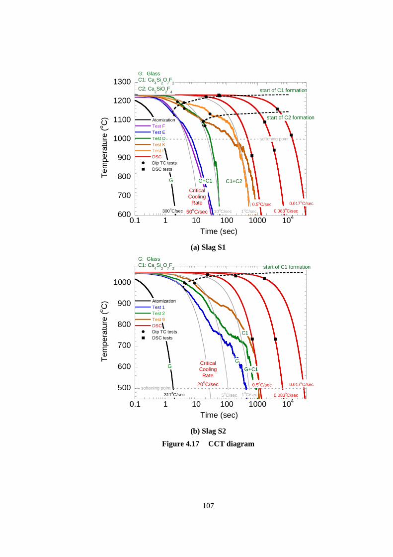
107

600

700

800

900

1000

1100

1200

1300

0.1 1 10 100 1000 104

AtomizationTest FTest ETest DTest KTest IDSCDip TC testsDSC tests

Tem

pera

ture

(o C)

Time (sec)

1oC/sec10oC/sec300oC/sec0.5oC/sec 0.017oC/sec

0.083oC/sec

G

G: GlassC1: Ca

4Si

2O

7F

2

C2: Ca2SiO

2F

4

G+C1 C1+C2

start of C1 formation


CriticalCooling

Rate

50oC/sec

softening point

(a) Slag S1

500

600

700

800

900

1000

0.1 1 10 100 1000 104

AtomizationTest 1Test 2Test 9DSCDip TC testsDSC tests

Tem

pera

ture

(o C)

Time (sec)

1oC/sec5oC/sec311oC/sec

0.5oC/sec 0.017oC/sec

0.083oC/sec

G

G: GlassC1: Ca

4Si

2O

7F

2

G+C1

C1


CriticalCooling

Rate

20oC/sec

G

softening point

(b) Slag S2

Figure 4.17 CCT diagram

108

(a) Plane polarized light (b) Cross polarized light (0o)

(c) Cross polarized light (45o) (d) Cross polarized light (90o)

Figure 4.18 Polarized light microscopy (slag H1)

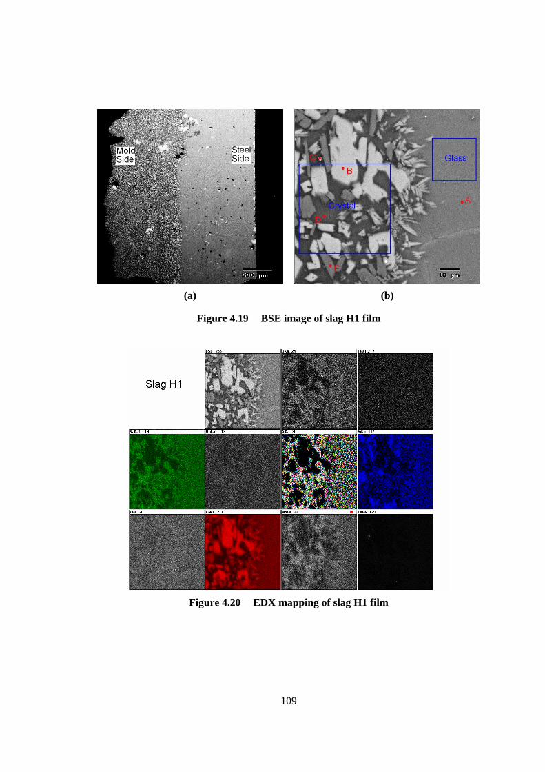
109

(a) (b)

Figure 4.19 BSE image of slag H1 film

Figure 4.20 EDX mapping of slag H1 film

110

0

1 104

2 104

3 104

4 104

5 104

6 104

7 104

0 1 2 3 4 5 6 7 8

TotalC

ount

s

Energy (keV)

CO

NaAl

Si

Ca

K Mn FeMg

0

1 104

2 104

3 104

4 104

5 104

6 104

7 104

0 1 2 3 4 5 6 7 8

Crystal area

Cou

nts

Energy (keV)

CO

NaAl

Si

Ca

K Mn FeMg

(a) Total (b) Crystal area

0

1 104

2 104

3 104

4 104

5 104

6 104

7 104

0 1 2 3 4 5 6 7 8

Glassy area

Cou

nts

Energy (keV)

CO

NaAl

Si

Ca

K Mn FeMg

0

1 104

2 104

3 104

4 104

5 104

6 104

7 104

0 1 2 3 4 5 6 7 8

Point A

Cou

nts

Energy (keV)

CO

NaAl

Si

Ca

K Mn FeMg

(c) Glassy area (d) Point A

0

2 104

4 104

6 104

8 104

1 105

0 1 2 3 4 5 6 7 8

Point B

Cou

nts

Energy (keV)

C O

Si

Ca

0

1 104

2 104

3 104

4 104

5 104

6 104

7 104

0 1 2 3 4 5 6 7 8

Point C

Cou

nts

Energy (keV)

CO

NaAl

SiCa

K Mn

Fe

Mg

(e) Point B (f) Point C

0

1 104

2 104

3 104

4 104

5 104

6 104

7 104

0 1 2 3 4 5 6 7 8

Point D

Cou

nts

Energy (keV)

CO Na

Al

Si Ca

K MnFe

Mg

0

1 104

2 104

3 104

4 104

5 104

6 104

7 104

0 1 2 3 4 5 6 7 8

Point E

Cou

nts

Energy (keV)

CO

Al

Si

Ca

(g) Point D (e) Point E

Figure 4.21 EDX spectrum of slag H1 film for points and areas in Figure 4.19(b)

111

CHAPTER 5. MODEL CALIBRATION

Having shown the model to be internally consistent, it cannot be used

quantitatively until it is calibrated to match measurements on the specific operating caster

of interest. This step is necessary because so many of the inputs to the model are

uncertain.

To date, the model has been calibrated to match many different casters, including

slabs at BHP LPD in Whyalla, South Australia; LTV Steel in Cleveland, OH[201], AK

Steel in Mansfield, OH[34], Allegheny Ludlum in Brackenridge, PA[202], Columbus

Stainless Steel in Middleburg[35], South Africa, Siderar in Argentina, and China Steel in

Taiwan, ROC; thin slabs at Nucor in Crawfordsville, IN[203] and POSCO in Seoul, S.

Korea[204]; blooms at BHP RBPD in Newcastle, New South Wales[205]; and billets at

POSCO Pohang in S. Korea[36]. In order to calibrate the model, it is simply run several

times, using trial and error to find values of the model parameters that allow the model

predictions to match all of the known measurements for a given set of casting conditions.

Those measurements can include the cooling water temperature rise, the time-average

temperature of any thermocouples embedded in the mold, the thickness profile of

breakout shells, the thickness of solidified mold powder layers and slag rims, and the

temperature histories of any thermocouples embedded in the strand.

Specifically, adjustments can be made to the velocity of the solid slag layer, the

value of the contact resistances down the mold, and even the thermal properties of the

mold slag. Other influential input parameters include the average powder consumption

rate and the average oscillation mark depth and width.

112

In a slab caster with properly designed taper, there should not be any air gap due

to shrinkage down the center of the wide face. This is because ferrostatic pressure pushes

the long, wide, weak shell against the mold to maintain as close a contact as possible.

This greatly simplifies model calibration when simulating a slice through the wide face of

the mold and shell.

Input parameters for the standard case, Table 5.1, were calibrated to match the

casting conditions of the 0.225m× 1.78m slabs of low-carbon steel cast at LTV Steel

Cleveland, OH, where cooling water temperature rise, mold thermocouple temperatures,

and breakout shell measurements were available[30, 206]. The steel composition is

0.044% C, 0.022%Mn, 0.006%S, 0.01%P, 0.009%Si and 0.049%Al.

5.1 Mold Cooling Water Temperature Rise

The first step in model calibration is to match the total heat extracted in the mold,

Q, with the measured temperature increase of the mold cooling water. The average rate of

heat extracted from the mold per unit surface area, Q, is found from:

int= ∆∑c

moldmold

VQ q tZ

(5.1)

This heat transfer rate should equal the temperature increase of the mold cooling water,

∆Twater, flowing through the “hot” channels, located adjacent to the slab width area:

int_ ρ

∆∆ = ∑ ch c

water hot channelsmold water pwater water ch ch

q L V tTC V w d

(5.2)

This equation assumes that the cooling water slots have locally uniform rectangular

dimensions, wch and dch, and spacing, Lch. Heat entering the hot face (between two water

113

channels) is assumed to pass straight through the mold to heat the water flowing through

the cooling channels.

To compare with the measured water temperature increase, the above prediction is

modified as follows to account for missing slots due to bolts or water slots, or slots that

are beyond the slab width, so do not participate in heat extraction:

_ _⋅ ⋅

∆ = ∆ ch ch chwater total channels water hot channels

w d W LT Ttotal channel area

(5.3)

Using reported slag properties and consumption rate (Table 5.1), heat flux was

calibrated to match the measured temperature rise of 7.1 deg C by adjusting the solid slag

speed ratio, fv, to 0.175. The corresponding temperature rise in just the hot channels is

predicted to be 7.5 deg C.

5.2 Mold Temperatures

The next step in calibration of CON1D is to further adjust the model parameters

to match the measurements of thermocouples embedded in the walls of the operating

casting mold. This step is very constrained, however, as every change that causes a local

increase in heat flux must be balanced by a corresponding decrease elsewhere, in order to

maintain the balance with the cooling water already achieved.

In this example, Table 5.1, the slag rim shape in region I was chosen to decrease

linearly from 0.8mm at the meniscus to 0.5mm at 15mm below the metal level, which is

near to the position of peak heat flux. The peak heat flux position should not be confused

with the location of peak mold temperature, which is usually about 35mm below the heat

flux peak (55 mm below the meniscus in this case). Assuming no air gap in the interface

for this wide face simulation, the contact resistances and scale thicknesses are other

114

adjustable input conditions to match the mold thermocouple measurements. Here a

0.02mm scale layer was assumed for the top 305mm, where special designed inserts had

been installed to increase the local cooling water velocity[206] and 0.01mm scale for the

bottom remainder of the mold. These thicknesses are in accordance with plant

observations that the hot region had a thicker scale layer[63].

Figure 5.1 compares the calibrated and measured temperatures at several locations

down the LTV mold. The thermocouples were all 18.8mm below the mold hot face. The

agreement indicates the calibration of the model for these typical casting conditions. This

figure also shows the predicted hot face and cold face temperature profiles. The sharp

change in temperature is due to a sudden increase in water channel depth, produced by

experimental inserts used in the trial[206]. Note that the observed scale layer greatly

increased the mold temperature, especially in the hot portion that contained the insert.

Based on this insight, steps were taken to improve water quality to prevent this scale and

improve mold life[206].

5.3 Shell Thickness

Having calibrated the model, the predicted shell thickness profile is compared

with measurements down a breakout shell that occurred under very similar castings

conditions, as given in Figure 5.2. Shell thickness is defined in the model by interpolating

the position between the liquidus and solidus isotherms with the temperature

corresponding to the specified solid fraction, fs, according to the phase fraction-

temperature relationship in Figure 3.2. In this sample case, fs=0.1, which is the only

adjustable parameter remaining for model calibration. This fraction is reasonable as

inter-dendritic liquid is held by surface tension during draining of the breakout.

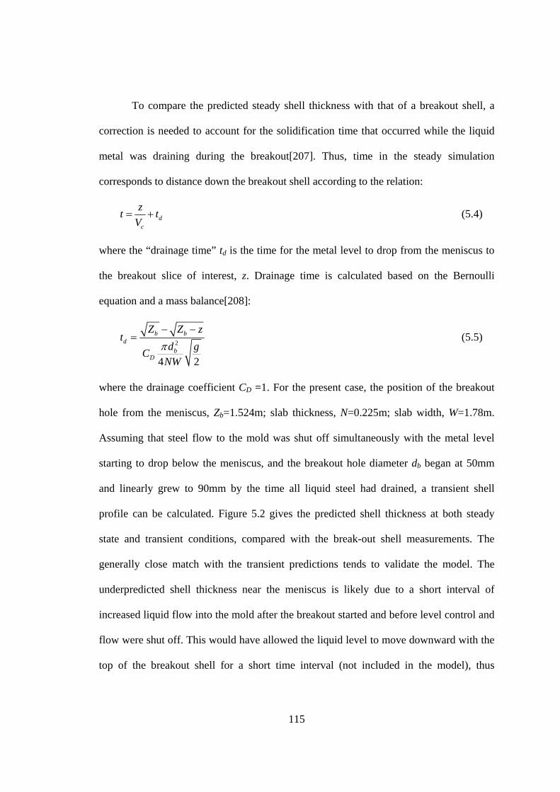
115

To compare the predicted steady shell thickness with that of a breakout shell, a

correction is needed to account for the solidification time that occurred while the liquid

metal was draining during the breakout[207]. Thus, time in the steady simulation

corresponds to distance down the breakout shell according to the relation:

= + dc

zt tV

(5.4)

where the “drainage time” td is the time for the metal level to drop from the meniscus to

the breakout slice of interest, z. Drainage time is calculated based on the Bernoulli

equation and a mass balance[208]:

2

4 2π− −

= b bd

bD

Z Z zt

d gCNW

(5.5)

where the drainage coefficient CD =1. For the present case, the position of the breakout

hole from the meniscus, Zb=1.524m; slab thickness, N=0.225m; slab width, W=1.78m.

Assuming that steel flow to the mold was shut off simultaneously with the metal level

starting to drop below the meniscus, and the breakout hole diameter db began at 50mm

and linearly grew to 90mm by the time all liquid steel had drained, a transient shell

profile can be calculated. Figure 5.2 gives the predicted shell thickness at both steady

state and transient conditions, compared with the break-out shell measurements. The

generally close match with the transient predictions tends to validate the model. The

underpredicted shell thickness near the meniscus is likely due to a short interval of

increased liquid flow into the mold after the breakout started and before level control and

flow were shut off. This would have allowed the liquid level to move downward with the

top of the breakout shell for a short time interval (not included in the model), thus

116

providing additional solidification time at the very top of the breakout shell. This effect is

commonly observed in breakout shells.

Growth of the shell naturally depends on both the interfacial and superheat fluxes.

The superheat distribution is important to the narrow face, as Figure 3.1 shows that the

two curves are of the same magnitude low in the mold where the hot molten steel jet

impinges against the solidifying shell. Figure 5.2 shows the shell thinning of the narrow

face due to this jet impingement effect.

Variation in the superheat flux is critical to shell growth down the narrow face

and off-corner regions, where problems such as inadequate taper sometimes produce

significant air gap(s). Together, the large superheat combined with decreased heat

transfer across the interfacial gap can reduce shell growth. This was the subject of a

significant study using the model, which was reported elsewhere[19].

5.4 Powder Layer Thickness

The model predicts the thickness and velocity profiles expected in the powder

layers in the interfacial gap. For example, Figure 5.3 shows the solid and liquid slag layer

thickness profiles expected for the standard conditions investigated here (Table 5.1). It

shows that the liquid slag layer runs out at 380mm below the meniscus, where the liquid

slag layer/steel shell interface temperature Ts’ drops below the slag solidification

temperature of 1045oC as shown in Figure 5.4. The total slag thickness continues to

increase while there is still liquid coming from the oscillation marks. This is indicated in

Figure 5.4, where the shell surface temperature at the oscillation mark roots, Ts, still

exceeds 1045oC at mold exit. Although no reliable slag samples were obtained from this

117

caster, these slag thickness predictions of 0.5 to 1.5mm are consistent with samples

measured at similar plants[31, 204].

5.5 Shell Surface Temperature

Typical model predictions of the surface temperature in the mold are shown in

Figure 5.4 for standard conditions. When liquid slag layer runs out at 380mm below the

meniscus (Figure 5.3), the liquid entrapped in the oscillation marks flows out and air fills

in. This increases the resistance of the oscillation mark, so the temperature difference

between the oscillation mark root and peak increases also, as shown in Figure 5.4.

After exiting the mold, the slab surface quickly reheats, and then fluctuates

greatly as it travels through the spray zones. Heat is extracted rapidly during contact with

the support rolls and when passing through the impingement zone of the cooling water

from the spray nozzles, which each cause great temporary drops in surface temperature.

Lacking accurate spray and roll contact heat transfer coefficients, calibration of

temperature predictions below the mold can be calibrated by adjusting the model

parameters froll and spray coefficients to match measurements such as roll cooling water

heat extraction rate, and thermocouple temperatures embedded in the strand. An example

of such calibration is shown in Figure 5.5 for casting conditions measured at China Steel

#1 slab caster in Taiwan, ROC, given in Table 5.2 and Table 5.3. The temperature

measurements were achieved by feeding a block containing several thermocouples into

the mold just before “tail-out” at the end of casting[37]. The thermocouple tips extending

through the bottom of the block were soon frozen into the strand. Being positioned before

the last several meters of steel before the end of the cast ensured that the recorded

temperature histories would be typical, while allowing the insulated tube of thermocouple

118

wires extending from the top of the block to follow the strand through the caster with

minimal damage. The distance of each thermocouple from the surface was measured

after sectioning the final product.

Internal temperature histories measured at three places beneath the surface are

included in Figure 5.5. Both surface thermocouples needed about 500 mm to heat up to

their surrounding shell temperatures, and later suffered from internal debonding, so their

results are reliable only between 500 and 3000 mm. The centerline thermocouple needed

almost 2m to heat up and appears to be accurate within 10oC. Both the internal

temperatures and the amplitude of their wiggles are roughly matched, indicating the

degree of calibration. Temperature fluctuations at the thermocouple location are quite

small, compared with the surface, which varies over 100oC over a single roll pitch. Near

the top of the caster, the greatest surface temperature drop occurs beneath each spray jet,

while a tiny dip occurs at each small region of direct contact with a support roll. Lower

in the caster, the relative size of the dips becomes closer, with deep sharp drops caused by

the high local heat extraction rate during roll contact under high ferrostatic pressure

Optical pyrometers are also useful for model calibration[176], but are adversely

affected by intermittent changes in surface scale emissivity and steam density from

evaporating spray water, so are most accurate when located below the spray chamber.

Attaching thermocouples directly to the strand surface is another difficult experimental

method that can be used for model calibration[46].

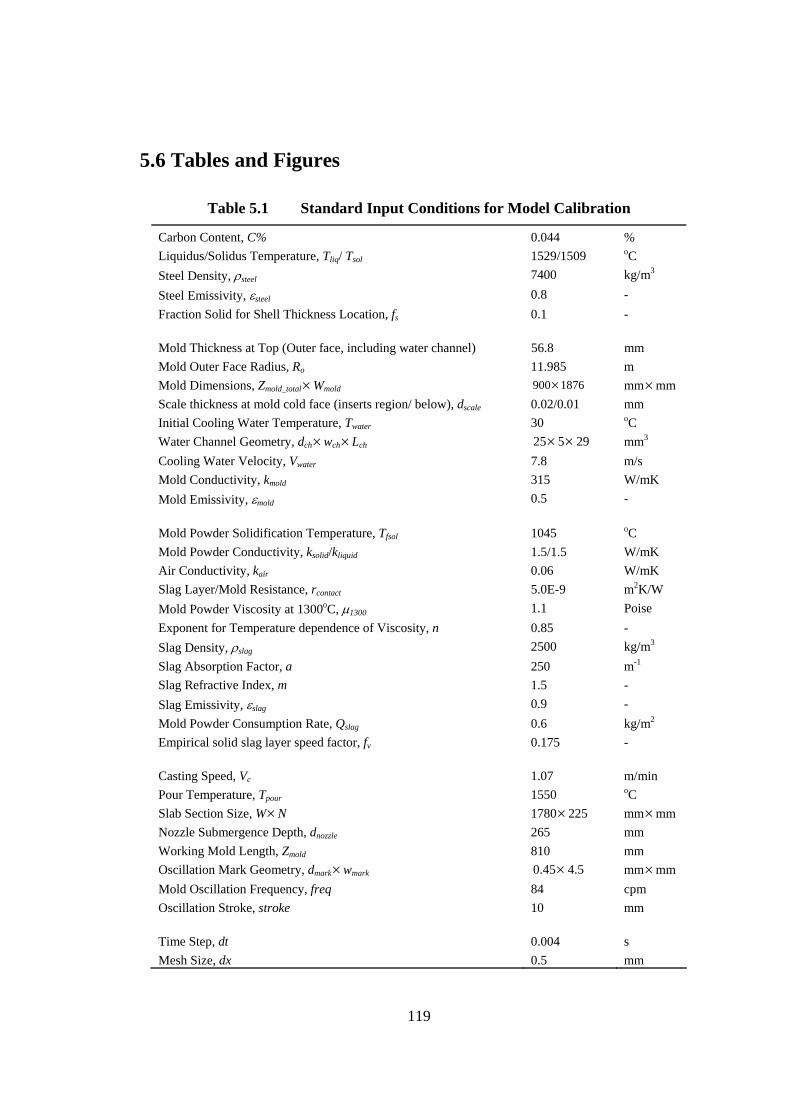
119


Table 5.1 Standard Input Conditions for Model Calibration

Carbon Content, C% 0.044 % Liquidus/Solidus Temperature, Tliq/ Tsol 1529/1509 oC Steel Density, ρsteel 7400 kg/m3

Steel Emissivity, εsteel 0.8 - Fraction Solid for Shell Thickness Location, fs 0.1 - Mold Thickness at Top (Outer face, including water channel) 56.8 mm Mold Outer Face Radius, Ro 11.985 m Mold Dimensions, Zmold_total ×Wmold 900 1876× mm×mm Scale thickness at mold cold face (inserts region/ below), dscale 0.02/0.01 mm Initial Cooling Water Temperature, Twater 30 oC Water Channel Geometry, dch×wch×Lch 25 5 29× × mm3 Cooling Water Velocity, Vwater 7.8 m/s Mold Conductivity, kmold 315 W/mK Mold Emissivity, εmold 0.5 - Mold Powder Solidification Temperature, Tfsol 1045 oC Mold Powder Conductivity, ksolid/kliquid 1.5/1.5 W/mK Air Conductivity, kair 0.06 W/mK Slag Layer/Mold Resistance, rcontact 5.0E-9 m2K/W Mold Powder Viscosity at 1300oC, µ1300 1.1 Poise Exponent for Temperature dependence of Viscosity, n 0.85 - Slag Density, ρslag 2500 kg/m3 Slag Absorption Factor, a 250 m-1 Slag Refractive Index, m 1.5 - Slag Emissivity, εslag 0.9 - Mold Powder Consumption Rate, Qslag 0.6 kg/m2

Empirical solid slag layer speed factor, fv 0.175 - Casting Speed, Vc 1.07 m/min Pour Temperature, Tpour 1550 oC Slab Section Size, W×N 1780×225 mm×mm Nozzle Submergence Depth, dnozzle 265 mm Working Mold Length, Zmold 810 mm Oscillation Mark Geometry, dmark×wmark 0.45 4.5× mm×mm Mold Oscillation Frequency, freq 84 cpm Oscillation Stroke, stroke 10 mm Time Step, dt 0.004 s Mesh Size, dx 0.5 mm

120

Table 5.2 Input Conditions for Sub-Mold Calibration (China Steel Case)

Carbon Content, C% 0.45 %

Mold Thickness at Top (including water channel) 51 mm

Initial Cooling Water Temperature, Twater 35 oC

Water Channel Geometry, ch ch chd w L× × 25 5 28× × mm3

Cooling Water velocity, Vwater 7.62 m/s

Casting Speed, Vc 0.55 m/min

Pour Temperature, Tpour 1510 oC

Slab Geometry, W N× 1560×270 mm×mm

Nozzle Submergence Depth, dnozzle 200 mm

Working Mold Length, Zmold 600 mm

Mold Oscillation Frequency, freq 120 cpm

Oscillation Stroke, stroke 4 mm

Cooling Water Temperature in Spray Zones, Tspray 35 oC

Spray Length of Spray Zone Nozzle, Lspray 0.05 m

Spray Zone Roll Contact Angle 7 Degree

Coefficients in Nozaki Eq.(3.58), A/b/c 0.3925/0.0075/0.55 -

Table 5.3 Input Spray Zone Variables (China Steel Case)

Zone #

Zone Starts at (mm) Roll # in Zone Roll Radius

(mm) Water Flow Rate

(l/min/row) Spray Width

(m) froll

1 600.0 2 70 27.5 1.3 0.05

2 906.9 5 70 14.86 1.2 0.05

3 1840.8 5 100 14.86 1.2 0.05

4 3034.3 5 125 11.84 1.2 0.2

5 4520.5 10 150 8.8 1.2 0.2

6 7977.9 10 175 7.15 1.2 0.2

7 11883.1 11 210 2.5 1.56 0.2

8 17050.7 18 240 0.0 1.56 0.2

26440.7 End of last spray zone

121

0

50

100

150

200

250

300

350

0 200 400 600 800

Mold Hot FaceMold Cold FaceCalibrated Thermocouple TemperatureMeasured Thermocouple Temperature

Tem

pera

ture

(o C)

Distance below Meniscus (mm)

Figure 5.1 Comparison of CON1D calibrated and measured mold temperature

0

5

10

15

20

25

30

35

0 200 400 600 800 1000 1200 1400

Wide Face MeasuredNarrow Face MeasuredCON1D Steady WFCON1D Steady NFCON1D Transient WFCON1D Transient NF

She

ll Th

ickn

ess

(mm

)


Figure 5.2 Comparison of CON1D predicted and measured shell thickness

122

0

0.2

0.4

0.6

0.8

1

1.2

1.4

0 100 200 300 400 500 600 700 800

Liquid LayerSolid LayerTotalS

lag

Laye

r Thi

ckne

ss (m

m)


Figure 5.3 Predicted slag layer thickness profiles

900

1000

1100

1200

1300

1400

1500

1600

0 100 200 300 400 500 600 700 800

Surface temperaure at oscillation mark root, Ts

Liquid slag/Steel shell interface, Ts'

She

ll S

urfa

ce T

empe

ratu

re (o C

)


Figure 5.4 Predicted shell surface temperature

123

900

1000

1100

1200

1300

1400

1500

1600

0 1000 2000 3000 4000 5000

Centerline12.5mm below surface10mm below surfaceSurface

She

ll Te

mpe

ratu

re (o C

)


Lines: CON1D CalculatedSymbols: TC measured

Figure 5.5 Shell temperature (China Steel Case)

124

CHAPTER 6. MODEL APPLICATIONS

The calibrated model has many applications for both design and operation of

continuous casting machines. Firstly, it can help to investigate the effect of various

process conditions on the fundamentals of mold heat transfer. Most parameters, such as

oscillation practice, powder type, casting speed, and steel grade, affect heat transfer in

several different ways, which can only be isolated and quantified independently using a

model. The model is currently being extended to predict liquid layer lubrication and solid

slag-layer fracture from excessive mold friction and the accompanying heat flux

variations,

The CON1D model is first used to simulate behavior for the typical casting

conditions listed in Table 3.3. To study the effect of slag type, three slags were chosen.

Figure 6.1 shows the viscosity curves vs. temperature assumed for these three slags,

which were chosen to match with slag viscosity data measured by Lanyi[100]. The

typical continuous casting Slag A might be crystalline or glassy (Slag A2 in Lanyi[100]);

Slag C is readily crystalline (Slag A6 in Lanyi[100]). Slag G is Slag C with 25%

additional alumina, which has a high tendency to be glassy[100]. The composition and

properties of these three slags are listed in Table 6.1.

The “lubrication consumption rate”, Qlub is a useful concept for comparing

different powder consumption rates. It is introduced here as the rate of slag consumption

neglecting the slag carried in the oscillation marks:

= −lub slag oscQ Q Q (6.1)

Oscillation marks filled with slag and moving at the casting speed consume slag

at the following rate, Qosc:

125

0.5 slag mark markosc slag osc

pitch

d wQ d

Lρ

ρ⋅ ⋅

= ⋅ = (6.2)

Thus, the total consumption rate of slag, Qslag, depends greatly on the oscillation

mark shape, while lubrication depends mainly on Qlub, and mold heat transfer depends on

both.

The liquid slag represented by Qlub acts to lubricate the mold-shell interface and

thereby lower friction. The CON1D model is run with different mold slags, consumption

rates and casting speeds to study the effect of mold powder properties and oscillation

practice. The related parameters are listed in Table 6.1 and Table 6.2.

6.1 Typical Results

Simulations were first run for typical low friction conditions, Case I (Table 3.3),

assuming that all solid slag is attached to the mold wall and constant lubrication

consumption rate Qlub, of 0.2kg/m2. At 1.0m/min casting speed, total consumption rate,

Qslag is 0.41kg/m2. Figure 6.2 shows typical results with Slag A. The mean heat flux in

the mold is 1.24MW/m2 and the shell thickness is 20.4mm at mold exit (based on a solid

fraction of 0.3). A uniform liquid slag layer of 0.29mm is predicted, Figure 6.2(d), while

the solid layer continually increases down the mold. Such a thick solid layer could build

up over time starting during initial mold filling with starter slag. Once it reaches steady

state, it does not consume any new mold powder. Increasing casting speed is naturally

predicted to raise heat flux but lower shell growth.

126

6.2 Crystallization Behavior

Figure 6.3 shows the cooling history of various points in the slag layer for Case I

with Slags A and G. The superimposed TTT curve of a conventional industrial mold slag

(7.9%Al2O3)[143] is used to estimate the onset of crystallization for Slag A. Figure 6.3(a)

predicts crystallization in most of the slag layer (including the oscillation marks) except

in the very thin (0.2mm) layer adjacent to the mold wall, which is quenched rapidly and

remains glassy. Extra alumina in the slag delays the onset of crystallization and increases

the temperature range of crystallization, so the TTT curve of a slag with 19.5%

Al2O3[144] is used to estimate the onset of crystallization for Slag G. Figure 6.3(b) shows

that no points within Slag G cross the TTT curve, so no crystalline phase is predicted.

This agrees with the assumption that Slag G tends to be glassy.

Shear stress and axial stress along the solid slag layer was plotted in Figure 3.15.

It shows that the solid slag layer is in compression almost everywhere. Therefore the

attached solid slag layer is stable and no fracture should occur. This can happen in

practice, as evidenced by the recovery of a solid slag layer attached to the mold wall after

one hour of casting, which contains trace elements only found in the starter slag

(consumed in the first few minutes)[157, 200]. The accompanying stable, thick liquid

layer ensures a very low friction force on the mold wall.

Figure 6.4(a) predicts the slag layer thicknesses of the glassy and crystalline slags,

assuming the same consumption rate and other conditions (Table 3.3). The glassy layer of

slag G is thinner due to its lower solidification temperature. Therefore it produces a

slightly higher heat flux and lower shell temperature than the crystalline slag, as shown in

Figure 6.4(b)(c). If the lower consumption rate that generally accompanies higher

127

viscosity slags in a real caster[6, 209] were taken into account, these differences would be

even greater. In either case, this prediction matches well-known measured behavior[6,

138, 210].

Note that the crystalline slag is predicted to have lower friction on the mold wall,

Figure 6.4(d). This is mainly because of its lower viscosity gradient at high temperature

(Figure 6.1), which helps the solid crystalline layer to stay attached to the mold wall and

prevent fracture.

6.3 Critical Slag Consumption Rate

Lowering the slag consumption rate, Qlub, leads to higher shear stress at the

liquid/solid slag interface. If friction on the mold side cannot balance the shear stress

along the solid/liquid interface, axial tensile stress must build up in the solid slag layer to

compensate. When axial stress in the solid slag exceeds the slag fracture strength, the

solid slag breaks and is dragged down the mold wall. The critical consumption rate is the

minimum consumption rate needed to keep solid slag attached to the mold wall without

breaking or sliding. In order to find it, the complete CON1D model was run several times

with different consumption rates, Case II, assuming slag fracture strength of 80MPa[211].

Figure 6.5 shows the axial stress and shear stress distribution of slags A and G along the

mold wall at their corresponding critical consumption rates. It shows that tensile axial

stress accumulates in the solid slag only when liquid shear stress exceeds maximum static

solid friction. In each case, fracture is predicted during the upstroke when axial stress just

exceeds the slag fracture strength. All stresses are compressive during the down stroke.

Slag G has 60% larger critical lubricating consumption rate, Qlub, 0.12kg/m2 than

Slag A, 0.075kg/m2. Slag C has similar behavior to Slag A, but with an even lower

128

critical Qlub, 0.05kg/m2. It confirms the general observations that crystalline slags are

more stable than glassy slags. Combined with their thicker layer and lower heat flux, this

may explain why such crystalline slags are better for depression and crack sensitive steel

grades[210, 212].

Another important difference between Slag A/C and G is the position of slag

fracture. As consumption rate lowers, the glassy slag drops below the critical

consumption rate first and fractures first near the mold exit. For crystalline slags A and C,

the solid slag layer fractures within 100mm near the meniscus. These results show that

the sharpness of the slag viscosity increase near the solidification temperature is more

important than the popular slag property, slag viscosity at 1300oC.

Figure 6.6 shows the heat flux and mold temperature of these two critical cases.

Relative to Case I, very high heat flux is predicted near the meniscus. This is also

indicated by the high mold temperature at that region. This also implies that in a real

caster, if an abnormal high mold temperature is observed near the meniscus, it may be

due to a temporary consumption rate drop regardless of slag type. This should also

correlate with solid slag breaking and moving down the mold wall. Slag fracture in turn

will cause temporary gaps, heat flux drops, and thermal stresses in the shell. The

phenomena of high meniscus heat flux and high variations are known to correlate with

strand defects[97, 213], which is consistent with the model prediction here.

6.4 Mold Friction

6.4.1 Attached Solid Slag Layer

When casting with a stable conventional consumption rate (Qslag=0.41kg/m2), the

model predicts a stable solid slag layer and a very low friction force. For the cases

129

studied here, the mold wall shear stress amplitude is 0.85MPa for slag A, and 2.52MPa

for slag G, which are far lower than reported measured friction data[33]. The high friction

force measured in operating casters likely comes from three possible causes: a moving

solid slag layer (and accompanying thinner liquid layer), excessive taper or

misalignment.

6.4.2 Moving Solid Slag Layer

If the liquid slag level at the meniscus varies, it cannot keep a steady flow into the

mold/strand gap even if the mold taper and alignment are reasonable and do not

contribute to friction. The solid slag layer may break and move along the mold wall,

accounting for part of the slag consumption. For a given consumption rate, the liquid slag

layer is thinner when the solid layer moves. This leads to higher heat flux and higher

friction and therefore perpetuates the slag fracture and motion. The fracture position

predicted for slag A (Case II with critical consumption rate) is near the meniscus. Thus,

the low viscosity liquid layer may quickly fill in the gap due to facture, and the solid slag

layer might reattach to the mold wall until the next fracture. For slag G, if the

consumption temporarily drops lower than the critical consumption rate, the solid slag

layer fracture will occur further above mold exit.

To model a moving solid slag layer, its average velocity is simply assumed to be

some small constant percentage of the casting speed, vf. In case III, assuming 5%fv ≈

produces total friction force predictions within the measured range of 15~23kPa[33].

Note the average “moving” solid slag layer velocity is actually the time average of a

highly transient process, calculated with an intermittent procedure of solid layer fracture,

movement and re-attachment. Most of the time, the solid layer still sticks to the mold

130

wall, so the shear stress can still be calculated based on liquid layer friction and the

maximum static friction between mold and solid layer. Figure 6.7 shows that both liquid

and solid moving layers are thinner than for the attached case. In particular, the liquid

slag layer gets thinner with distance down the mold and nearly runs out by mold exit.

This increases friction greatly. (Appendix I gives a complete list of input and output files

of the run with moving solid slag layer with Slag A)

6.4.3 Friction Variation during an Oscillation Cycle

Figure 6.8(a) shows the mold velocity and casting speed profile during half of one

oscillation cycle. It shows that at one instant, 0.24second, the mold velocity equals the

casting speed, so there is no shear stress. After that time, the mold moves down faster

than the shell during the period of “negative strip”. Thus, the stress acting on the slag

layer shifts from tension to compression during that instant. Figure 6.8 also shows that

the shear stress on the mold wall with a “moving” solid slag layer, (c), is much higher

than with an attached layer, (b). Shear stress increases with distance along the mold

length, and the transition from tension to compression becomes sharper for a moving

layer. In the upper mold, liquid slag controls the friction between mold and shell, so the

shear stress is nearly sinusoidal. In the lower mold region, the solid slag layer controls

friction and the shear stress profile tends toward a square wave.

Figure 6.9 shows the shear stress down the mold at different times during the

oscillation cycle. For all times, there is a transition from curved to straight, where liquid

slag layer control transfers to solid slag layer control. The "average" is the mean of the

absolute values of all the shear stresses over the whole oscillation cycle, and is very near

to the curve when Vm is zero. This means that the average friction force can be estimated

131

with a simple static mold model. Integrating the shear stress over each mold face at each

instant gives the total friction force history during each oscillation cycle, as shown in

Figure 6.10 for different cases.

6.4.4 Total Mold Friction Force

Figure 6.10 shows that the friction due to shear stress is very small if the solid

slag layer is attached and there are no other sources of friction. Friction with an

intermittent attached solid layer is 10X larger and has a sharper transition from tension to

compression. Another possible cause of high friction may be squeezing of the steel shell

due to excessive narrow face taper. This is most likely when the shell temperature is high

and shrinkage is small at high casting speed. A rough estimation of the magnitude of this

friction is 15kN on each narrow face, based on Eqs.(3.51),(3.52), assuming buckling

happens over the last 10mm (h=10mm) near mold exit, shell thickness b=20mm,

Leff=600mm, E=25GPa at 1100oC. This corresponds to an average friction stress over a

800mm long 230mm thick and 1500mm wide slab mold of 10kPa, which is similar to

measured data[33]. Figure 6.10 shows that the friction force during an oscillation cycle

for excessive taper can be identified by its almost-square shape. In contrast, liquid slag

lubrication produces a smooth curve with a very gradual transition. Thus the

lubrication/friction state of the mold can be identified from the shape of the friction force

curve during an oscillation cycle in addition to its magnitude. Misalignment friction

curves are expected to be curved according to gradual changes in its extent during the

cycle.

132

6.5 Other Applications

The model can make predictions of potential quality problems, which have more

relevance in practice than simple heat transfer. For example, a warning of possible

boiling in the cooling water channels is issued when the mold surface temperature

exceeds the pressure-dependent water boiling temperature. The model is also being used

to make other warnings such as breakout danger from excessive shell thinning at mold

exit, and crack formation etc. Finally, the model should predict optimum casting

conditions to avoid problems, whenever possible. Initial features of the model toward this

goal include a prediction of ideal mold taper. Together with other resources, CON1D is a

powerful tool to investigate the cause and prevention of quality problems and to

investigate potential design and operation improvements prior to costly experimental

implementation.

6.5.1 Boiling Prediction

The model issues a warning that boiling is possible, if the mold cold face

temperature exceeds the boiling temperature for the given operating pressure in the

cooling water channels[214]:

( ) ( )( )0.27: 100 / 0.10135>o

coldBoiling if T C P MPa (6.3)

Boiling in the water channels changes the rate of heat removal and causes

temperature fluctuations that together pose a serious potential quality problem. Figure 5.1

shows that boiling is indeed possible for the conditions investigated here. This is due to

the 0.02mm thick layer of scale on the mold cold face near the meniscus, which raises the

mold face temperature ~70oC. On the other hand, adding a 0.5 mm thick protective Ni

133

coating to the hot face is predicted to have only a minimal effect on heat flux and cold

face temperature. The CON1D model is ideal for quantifying effects such as these.

6.5.2 Breakout Analysis

The model can be used to help understand how a breakout may have arisen.

Sticker breakouts are easily identified by their characteristic effect on mold thermocouple

histories. Other breakouts, such as those caused by inadequate taper, can be more difficult

to identify. For example, the model could be used to determine whether a given narrow-

face breakout was more likely caused by excessive superheat resulting from a clogged

nozzle, or from insufficient mold taper, causing an excessive gap. Either condition could

produce a narrow-face shell that is too hot and thin to have the hot strength needed to

avoid rupture. Further calibration may allow the model to accurately warn of a potential

breakout when shell growth is predicted to fall below a critical value. Initial work

towards this end is reported elsewhere[59].

6.5.3 Crack Formation Analysis

As with previous continuous casting models, CON1D can be used to locate where

defects are formed. Hot tear cracks form near the location of the solidus isotherm is

tracked by CON1D. For example, by accurately predicting the shell thickness exiting the

mold, the model can identify whether a subsurface crack formed in or below the mold.

This can be difficult to tell, particularly near the narrow face, where shell growth is

slower. Here, a crack forming below the mold might appear to have formed in the mold

without an accurate calculation of shell growth that incorporates superheat delivery. The

model can also simulate phenomena below the mold, such as reheating of the shell

134

surface, which can lead to surface cracks. Sub-mold bulging and crack formation requires

accurate prediction of the temperature variation between rolls, so the model is useful for

designing spray water-cooling systems.


Table 6.1 Slag Composition and Properties

Slag CaO SiO2 Al2O3 MgO Na2O K2O F2 FeO MnO B2O3 Tfsol n 1300µ

wt% wt% wt% wt% wt% wt% wt% wt% wt% wt% oC - P

A 32.3 36.4 8.9 0.7 5.0 1.9 8.3 3.0 - 3.4 950 1.6 4.3

G 27.5 30.3 21.4 0.9 5.6 - 12.0 1.1 1.3 - 850 3.2 5.0

C 34.8 38.3 0. 5 1.2 7.1 - 15.2 1.4 1.6 - 980 1.6 1.7

Table 6.2 Case Study Parameters

Case I Case II Case III

Lubrication Consumption, Qlub: 0.2kg/m2 critical 0.2kg/m2

Solid Layer Status: attached attached moving

1

10

100

1000

104

105

106

900 1000 1100 1200 1300 1400

Slag A

CON1D: µ1300

=4.3Poise, Tfsol

=950oC, n=1.6

Slag G (Glassy)

CON1D: µ1300

=5.0Poise, Tfsol

=850oC, n=3.2

Slag C (Crystalline)

CON1D: µ1300

=1.7Poise, Tfsol

=980oC, n=1.6

Vis

cosi

ty (P

oise

)

Temperature (oC)

Symbols: measurements from Lanyi

Figure 6.1 Mold slag viscosities used in cases study

135

0

0.5

1

1.5

2

2.5

3

3.5

0 100 200 300 400 500 600 700 800

Hea

t Flu

x (M

Pa)


0

200

400

600

800

1000

1200

1400

1600

0 100 200 300 400 500 600 700 800

Shell SurfaceMold Hot FaceMold Cold Face

Tem

pera

ture

(o C)


(a) Heat flux (b) Shell and mold temperature

0

5

10

15

20

0 100 200 300 400 500 600 700 800

Shel

l Thi

ckne

ss (m

m)


0

0.5

1

1.5

2

0 100 200 300 400 500 600 700 800

Liquid layerSolid layerTotal

Sla

g La

yer T

hick

ness

(mm

)


(c) Steel shell thickness (d) Slag layer thickness

Figure 6.2 Typical results of Case I with slag A

136

200

400

600

800

1000

1200

1400

0 100 200 300 400 500 600 700 800

0.2mm0.4mm0.6mm0.8mm1.0mm

Tem

pera

ture

(o C)


Distance from mold hot faceSlag in Osc. marks

200

400

600

800

1000

1200

1400

1 10 100 1000


Tem

pera

ture

(o C)

Time (s)

7.9% Al2O

3

Slag in Osc. marksDistance from mold hot face

(a) Slag A (crystalline)

200

400

600

800

1000

1200

1400

0 100 200 300 400 500 600 700 800


Tem

pera

ture

(o C)

Distance Below Mensicus (mm)

Distance from mold hot faceSlag in Osc. marks

200

400

600

800

1000

1200

1400

1 10 100 1000


Tem

pera

ture

(o C)

Time (s)

Distance from mold hot face

Slag in Osc. marks

19.5% Al2O

3

(b) Slag G (glassy)

Figure 6.3 Slag layer cooling history with TTT curves

137

0

0.5

1

1.5

2

0 100 200 300 400 500 600 700 800

Slag GSlag C

Tota

l Sla

g La

yer T

hick

ness

(mm

)


0

0.5

1

1.5

2

2.5

3

0 100 200 300 400 500 600 700 800

Slag GSlag C

Hea

t Flu

x (M

Pa)


(a) Slag layer thickness (b) Heat flux

1000

1100

1200

1300

1400

1500

1600

0 100 200 300 400 500 600 700 800

Slag GSlag C

Shel

l Tem

pera

ture

(o C)


0

1

2

3

4

0 100 200 300 400 500 600 700 800

Slag GSlag C

Shea

r Stre

ss o

n M

old

Wal

l (kP

a)


maximum up-stroke

(c) Shell temperature (d) Mold friction

Figure 6.4 Effects of slag type

138

-2

-1

0

1

2

3

0 20 40 60 80 100

up, sol/liq interfaceup, mold sidedown, sol/liq interfacedown, mold sideMaximum Static Friction on Mold Wall

She

ar S

tress

(kP

a)


axial stress builds up

-20

0

20

40

60

80

0 100 200 300 400 500 600 700 800

Maximum Up Stroke

Maximum Down Stroke

Axi

al S

tress

in S

olid

Sla

g La

yer (

kPa)


slag fracture strength: 80kPa

(a) Slag A (crystalline)

-10

-5

0

5

10

15

20

25

30

0 100 200 300 400 500 600 700 800

up, sol/liq interfaceup, mold sidedown, sol/liq interfacedown, mold sideMaximum Static Friction on Mold Wall

She

ar S

tress

(kP

a)


axial stress builds up

-20

0

20

40

60

80

0 100 200 300 400 500 600 700 800

Maximum Up StrokeMaximum Down Stroke

Axi

al S

tress

in S

olid

Sla

g La

yer (

kPa)


slag fracture strength: 80kPa

(b) Slag G (glassy)

Figure 6.5 Effect of Slag type on axial stress build up

in solid layerfor critical Qlub(Case II)

0

1

2

3

4

5

6

0 100 200 300 400 500 600 700 800

Slag A, Qlub

=0.075kg/m2

Slag A, Qlub

=0.2kg/m2

Slag G, Qlub

=0.12kg/m2

Slag G, Qlub

=0.2kg/m2

Hea

t Flu

x (M

Pa)


0

100

200

300

400

500

0 100 200 300 400 500 600 700 800

Slag A: Hot FaceSlag A: Cold FaceSlag G: Hot FaceSlag G: Cold Face

Mol

d Te

mpe

ratu

re (o C

)

Distance Below Meniscus (mm) (a) Heat flux (b) Mold temperature

Figure 6.6 Comparison of heat flux and mold temperature

with critical consumption rate (Case II)

139

0

0.2

0.4

0.6

0.8

1

1.2

1.4

0 100 200 300 400 500 600 700 800

Liquid layerSolid layerTotal

Sla

g La

yer T

hick

ness

(mm

)


Figure 6.7 Slag layer thickness with “moving” solid layer (Case III with Slag A)

140

-40

-20

0

20

400 0.09 0.18 0.27 0.36

Vc

Vm

Vel

ocity

(mm

/s)

Time (s)

(a) Casting speed and mold velocity

-0.5

0

0.5

1

0 0.09 0.18 0.27 0.36

300500800S

hear

Stre

ss (k

Pa)

Time (s)

Distance belowmeniscus (mm)

(b) Attached solid layer (Case I)

-20-10

01020

0 0.09 0.18 0.27 0.36

300500800S

hear

Stre

ss (k

Pa)

Time (s)


(c) “Moving” solid layer (Case III)

Figure 6.8 Velocity and shear stress during half oscillation cycle (Slag A)

141

-20

-10

0

10

20

30

0 100 200 300 400 500 600 700 800

0 (max. up)1/81/4 (V

m=0)

3/81/2 (max. down)Avg

She

ar S

tress

(kP

a)


fraction of cycle(0.72sec period)

Figure 6.9 Shear stress down the mold wall with “moving” solid layer (Slag A)

-20

0

20

0 0.09 0.18 0.27 0.36

-2

0

2

Attached solid layerMoving solid layerAttached layer w/ excessive taperFr

ictio

n Fo

rce

(kN

)(m

ovin

g/ex

cess

ive

tape

r)

Time (s)

Fric

tion

Forc

e (k

N)

(atta

ched

laye

r)

(a) Casting speed and mold velocity

-20

0

20

-4 -2 0 2 4

-2

0

2

Attached solid layerMoving solid layerAttached layer w/ excessive taper

Fric

tion

Forc

e (k

N)

(mov

ing/

exce

ssiv

e ta

per)

Mold Displacement (mm)

Fric

tion

Forc

e (k

N)

(atta

ched

laye

r)

(b) Attached solid layer (Case I)

Figure 6.10 Friction force over oscillation cycle (Slag A)

142

CHAPTER 7. SLAG CONSUMPTION AND CASTING SPEED STUDY

7.1 Effect of Casting Speed on Heat Transfer and Shell Growth

As an example to illustrate the use of the model to understand fundamental

phenomena in the mold, simulations were performed to investigate just two of the many

interdependent parameters: casting speed and mold powder consumption. It is well

known that increasing casting speed causes changes to other parameters, such as

decreased mold powder consumption rate and shallower oscillation marks. To investigate

the effect of increasing casting speed in a typical real caster, oscillation frequency was

increased proportionally with speed, according to plant practice, and oscillation mark

depth was decreased, such that the negative strip ratio and the lubrication consumption

rate , Qlub remained constant.

To investigate the effect of mold powder consumption rate, an intermediate case

of standard (low) casting speed with decreased consumption rate is also included. The

three cases in this study are listed in Table 7.1, with other conditions given in Table 5.1.

The lubrication consumption rate for all 3 cases is 0.4kg/m2.

Figure 7.1 presents the heat flux profiles down the mold wide face calculated for

all three cases. Decreasing the powder consumption rate at constant casting speed (Case

2) is seen to increase heat flux in the top portion of the mold, relative to standard

conditions (Case 1). This is because the average thickness of the slag layers decreases,

thus lowering the interfacial resistance. This effect diminishes with distance down the

mold, (as the importance of interfacial resistance to heat transfer decreases relative to that

from increasing steel shell thickness).

143

The practical case of increasing casting speed and simultaneously decreasing total

powder consumption rate and oscillation mark depth (Case 3) also increases heat flux

toward the bottom of the mold. This is due to the lower thermal resistance of a thinner

steel shell produced with less solidification time, which becomes increasingly important

with distance down the mold. The net result of increasing casting speed (comparing Case

3 with Case 1) is to increase heat flux almost uniformly down the mold. This is reflected

in uniformly higher mold temperatures, as seen in the model predictions in Figure 7.2.

This prediction also matches mold thermocouple measurements obtained for Case 3

conditions, as included in Figure 7.2. The higher speed leads to a thinner steel shell and

higher steel surface temperature so the liquid slag layer persists further down the mold, as

shown in Figure 7.3, Figure 7.4 and Figure 7.5 respectively. But the higher heat flux for

higher casting speed also lowers the shell surface temperature, which partially cancels the

effect of higher temperature due to thinner shell. For these cases, the surface temperatures

at the oscillation marks root near mold exit are almost the same, as shown in Figure 7.4

and Figure 7.6. Figure 7.6 compares the shell temperature profiles at mold exit.

The model is suited to many further fundamental parametric studies of this kind.

For example, steel grade affects the average oscillation mark size, powder consumption

rate, air gap size due to thermal contraction (narrow face), and steel strength. Mold

powder properties and oscillation practice have similar interdependent effects. The effect

of oscillation mark depth, for example, is quantified in a model application reported

elsewhere[201].

For the sample cases, the higher speed causes a hotter shell with less shrinkage,

shown in Figure 7.7, so needs slightly less narrow face mold taper. The shrinkage εth1,

144

based on surface temperature only, is generally less than εth2, and is almost independent

of casting speed, due to the cancellation effect discussed previously. With a linear taper,

the narrow-face shell attempts to shrink away from the upper portion of the mold, while it

pushes against the lower portion of the mold. To match the shrinkage, it is clear that taper

should be increased high in the mold and decreased lower down. Mold distortion,

viscoplastic creep of the steel, and other factors should also be taken into account when

designing a non-linear mold taper. These calculations require sophisticated thermal-stress

models, to calculate temperatures, stresses, and shrinkage, including the formation of an

air gap near the corners, and its effect on heat flow across the mold/shell interface. The

calibrated CON1D model is currently being used to provide calibrated heat transfer data

to these models to evaluate and improve taper optimization.

7.2 Effect of Slag Properties on Critical Consumption Rate

The most important parameter affecting slag shear stress and fracture was found

to be the liquid slag consumption rate. So long as consumption rate exceeds a minimum

critical rate, the slag will not fracture. A parametric study was conducted on the minimum

critical consumption to keep a stable attached solid slag layer using conditions in Table

3.3. Doubling the fracture strength of the crystalline mold slag allows the critical Qlub for

slag A to decrease by only 7% and delays the fracture position from 60mm to 100mm

below the meniscus. The fracture strength has even less effect for slag G. The effects of

slag Poisson’s ratio, liquid slag pool depth, and mold thickness on critical consumption

rate were negligible.

Maintaining a high mold/slag friction coefficient is important to lowering the

critical consumption. As shown in Figure 7.8, especially for slag G, when the friction

145

coefficient is lower than 0.15, the slag layer can fracture, even for a stable conventional

consumption rate.

Oscillation marks act as an extra resistance layer between the liquid slag layer and

the steel shell. Thus they slightly lower temperature in the liquid layer, which leads to

higher viscosity liquid, higher shear stress, easier flux fracture and higher critical

consumption. Specifically, 0.45mm*4.5mm oscillation marks cast at 1.0m/min increase

Qlub by 0.01kg/m2 for both slags (15% for slag A and 9% for slag G) relative to cases

with no oscillation marks

7.3 Effect of Casting Speed on Critical Consumption Rate

The influence of casting speed on mold friction and interface heat flux has been

investigated in a parametric study. Based on Case I, the casting speed was varied from

1.0m/min to 5.0m/min. The stroke was fixed at 7.8mm, and oscillation frequency

adjusted to keep a constant negative strip ratio of 0.3 and a constant pitch length of

12mm. Negative strip time thereby decreases with increasing casting speed, so oscillation

mark depth decreases[215]. The powder consumption rate thus decreases due to the

shallower oscillation marks and higher oscillation frequency[216]. Oscillation mark depth

becomes negligible when casting speed is greater than 2m/min. Table 7.2 gives the mold

oscillation parameters used. Those parameters are chosen based on some previous plant

measurements of oscillation marks depth[215] and total mold powder consumption

rate[15, 31, 97, 217] as shown in Figure 7.9 and Figure 7.10.

Figure 7.10 also compares measured consumption rates[15, 31, 97, 217] with

critical consumption rates calculated in this study. Measured consumption rates exceed

the critical rates, which indicates that slag fracture should be a rare transient event. If the

146

total consumption rate can be steadily maintained, the strand should be well lubricated

and a stable solid slag layer should remain attached to the mold. Figure 7.10 shows that

measured consumption rates decrease with increasing casting speed. When there is

significant consumption by the oscillation marks, Qosc, the critical consumption also

decreases with increasing casting speed. This is because oscillation mark depth decreases,

carries less slag and increases the lubrication consumption component, thus helping to

keep the solid layer attached to the mold wall as explained above. However, at higher

casting speed (>2m/min), when the oscillation mark effect is negligible, the critical

consumption rate increases slightly with casting speed.

Figure 7.11 shows two opposing effects of casting speed on solid slag fracture,

excluding oscillation marks and their effects. Increasing casting speed increases the

velocity difference between mold and shell, which tends to increase friction. It also

increases shell surface temperature, which tends to decrease slag viscosity and friction.

For slag A, the first effect prevails, so the slag always fails near the meniscus and higher

casting speed is more dangerous to slag fracture. To be specific, increasing Vc from

1.0m/min to 2.0 m/min, requires the critical Qlub to increase by 25%. Also, the fracture

position occurs closer to the meniscus (moving from 60mm to 30mm). When the critical

fracture position is near to the mold exit, such as slag G at less than 3.0m/min, the effect

of higher surface temperature predominates, so higher casting speed helps to avoid slag

fracture, as shown in Figure 7.11(b). Thus, increasing casting speed from 1.0m/min to

2.0m/min decreases critical Qlub by 8%. However, further increasing casting speed above

3.0m/min causes the critical fracture position to move to near the meniscus, and increases

the critical Qlub as for slag A.

147

Note that the minimum critical consumption rate occurs at intermediate speed

(~2m/min) for the conditions of the study with Slag G, which is the safest speed for slag

layer stability. Measured consumption rates exceed the calculated critical consumption

rates by the largest factor (~3X) for this intermediate speed. Safety margins are less at

both lower speed and higher speed. At very high speed, ~5m/min, measured

consumptions approach critical levels. This indicates that solid slag layer stability

becomes a general problem at high speed (unless consumption or another condition

assumed here is changed).

Figure 7.12 compares the average heat flux with measured and fitted data[43, 59,

72, 218]. Average mold heat flux increases with higher casting speed (shorter dwell

time), with lower consumption rate or with a moving solid slag layer. Note that the

average heat flux of the cases with moving slag or with critical consumption rate (just

about to move) almost hit the upper bound of measurements. High and variable heat flux

is another indication of slag layer fracture.

7.4 Effect of Casting Speed on Friction Stress

Finally, CON1D was run with a detached solid slag layer assumed to be moving at

an average velocity of 5% of the casting speed (Case III). The lubrication consumption

rate Qlub was assumed to remain the same, 0.2kg/m2, for all cases. The solid friction force

with moving slag is much higher than for the attached cases, and increases with

decreasing casting speed. These predictions compare with measured data[33], as shown

in Figure 7.13. The agreement at lower casting speed is consistent with the prediction that

solid slag fracture and movement increases at lower speed. The high friction measured at

high speed might be due to other friction sources such as excessive mold taper. Also note

148

that for the same average solid layer moving speed, glassy slag has higher friction than

crystalline slag. It is interesting speculate that the drop in friction at intermediate speed

might correspond to the minimum in critical consumption rate and maximum safety

factor predicted in this work. It implies that solid slag layer fracture may be more likely

at both low and high casting speed, perhaps increasing the higher average solid layer

moving speed, which would increase friction. This is consistent with measurements in

Figure 7.13.


Table 7.1 Parametric Study Conditions for Effect of Casting Speed

Casting Speed

Vc (m/min)

Oscillation frequency freq (cpm)

Total Consumption Rate Qslag (kg/m2)

Osc. Mark Size

mark markd w× (mm2)

Case 1 1.07 84 .60 .45×4.5

Case 2 1.07 84 .56 .45×4.5

Case 3 1.25 98 .56 .40×4.0

Table 7.2 Mold Oscillation Practice with Casting Speed

Casting Speed, Vc

Oscillation frequency, f

Negative Strip Time, NST

Negative Strip ratio, NS%

Osc. Mark,

mark markd w×

Osc. Marks Consumption, Qosc

m/min cpm s - mm×mm kg/m2

1.0 83.3 0.24 0.3 .45*4.5 0.21

1.3 108.3 0.19 0.3 .30*3.0 0.094

1.6 133.3 0.15 0.3 .16*1.6 0.027

2.0 166.7 0.12 0.3 0*0 0

3.0 250.0 0.08 0.3 0*0 0

5.0 416.7 0.05 0.3 0*0 0

149

1

1.5

2

2.5

3

0 100 200 300 400 500 600 700 800

Case 1: 1.07m/min, CONS=0.6kg/m2

Case 2: 1.07m/min, CONS=0.56kg/m2

Case 3: 1.25m/min, CONS=0.56kg/m2H

eat F

lux

(MW

/m2 )


Figure 7.1 Effect of casting speed and powder

consumption on the heat flux profile

40

80

120

160

200

0 200 400 600 800

Case 1: 1.07m/minCase 3: 1.25m/min

Tem

pera

ture

(o C)


Lines: CON1D PredictionsSymbols: Mesaured Data

Figure 7.2 Effect of casting speed on mold temperature

150

0

5

10

15

20

25

0 100 200 300 400 500 600 700 800

Case 1: 1.07m/minCase 3: 1.25m/min

She

ll Th

ickn

ess

(mm

)


Figure 7.3 Effect of casting speed on steel shell thickness

900

1000

1100

1200

1300

1400

1500

1600

0 100 200 300 400 500 600 700 800

Case 1: 1.07m/min (Osc. Mark Root)Case 1: 1.07m/min (Liquid Slag/Steel Shell Interface)Case 3: 1.25m/min (Osc. Mark Root)Case 3: 1.25m/min (Liquid Slag/Steel Shell Interface)

She

ll S

urfa

ce T

empe

ratu

re (o C

)


Figure 7.4 Effect of casting speed on steel shell surface temperature

151

0.4

0.6

0.8

1

1.2

0 100 200 300 400 500 600 700 800

Case 1: 1.07m/min, Solid LayerCase 1: 1.07m/min, TotalCase 3: 1.25m/min, Solid LayerCase 3: 1.25m/min, Total

Sla

g La

yer T

hick

ness

(mm

)


Figure 7.5 Effect of casting speed on slag layer thickness

1000

1100

1200

1300

1400

1500

1600

0 5 10 15 20 25

Case 1: 1.07m/min

Case 3: 1.25m/min

She

ll Te

mpe

ratu

re (o C

)

Distance into Steel Shell (mm)

Figure 7.6 Effect of casting speed on steel shell temperature profile at mod exit

152

0

0.2

0.4

0.6

0.8

1

1.2

1.4

1.6

0 100 200 300 400 500 600 700 800

Case 1: 1.07m/min, εth1




She

ll S

hrin

kage

(%)


Figure 7.7 Effect of casting speed on steel shell shrinkage

0

0.1

0.2

0.3

0.4

0.5

0 0.2 0.4 0.6 0.8 1

Slag A: Qslag

Slag A: Qlub

Slag G: Qslag

Slag G: Qlub

Crit

ical

Con

sum

ptio

n R

ate

(kg/

m2 )

Friction Coefficient

measured consumption rate range

Vc=1.0m/min

Qosc

=0.21kg/m2

Figure 7.8 Effect of friction coefficient on critical consumption rate

153

0.2

0.3

0.4

0.5

0.6

0.7

0.8

0.15 0.18 0.21 0.24 0.27

HamagamiCON1D

Max

imum

Dep

th o

f Osc

. Mar

k (m

m)

Negative Strip Time (s)

Vc=1.0m/min

Vc=1.3m/min

Vc=1.6m/min

Figure 7.9 Maximum oscillation mark depth

0

0.1

0.2

0.3

0.4

0.5

1 2 3 4 5

70cpm -Inagaki100cpm -Inagaki100cpm -Ho97-174cpm -Suzuki189cpm-Hiraki/NakajimaCON1D Q

slag with conventional consumption

CON1D Qlub

with conventional consumption

CON1D Qslag

with criticall consumption(Slag A)

CON1D Qlub

with criticall consumption(Slag A)

CON1D Qslag

with critical consumption(Slag G)

CON1D Qlub

with criticall consumption(Slag G)

Mol

d P

owde

r Con

sum

ptio

n (k

g/m

2 )

Casting Speed (m/min)

83.3cpm

103.3cpm

133.3cpm

Figure 7.10 Powder consumption rates

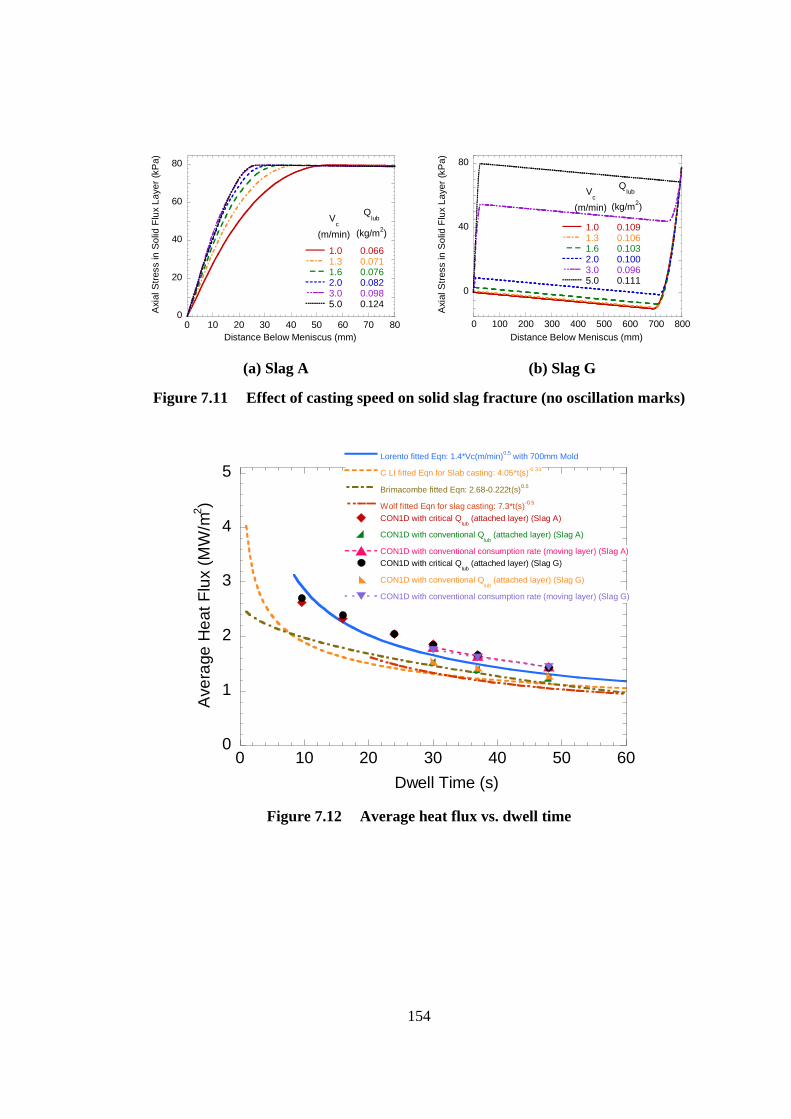
154

0

20

40

60

80

0 10 20 30 40 50 60 70 80

1.0 0.066 1.3 0.071 1.6 0.076 2.0 0.082 3.0 0.098 5.0 0.124A

xial

Stre

ss in

Sol

id F

lux

Laye

r (kP

a)


Vc

(m/min)

Qlub

(kg/m2)

0

40

80

0 100 200 300 400 500 600 700 800

1.0 0.109 1.3 0.106 1.6 0.103 2.0 0.100 3.0 0.096 5.0 0.111

Axi

al S

tress

in S

olid

Flu

x La

yer (

kPa)


Vc

(m/min)

Qlub

(kg/m2)

(a) Slag A (b) Slag G

Figure 7.11 Effect of casting speed on solid slag fracture (no oscillation marks)

0

1

2

3

4

5

0 10 20 30 40 50 60

Lorento fitted Eqn: 1.4*Vc(m/min)0.5 with 700mm Mold

C LI fitted Eqn for Slab casting: 4.05*t(s)-0.33

Brimacombe fitted Eqn: 2.68-0.222t(s)0.5

Wolf fitted Eqn for slag casting: 7.3*t(s)-0.5

CON1D with critical Qlub

(attached layer) (Slag A)

CON1D with conventional Qlub

(attached layer) (Slag A)

CON1D with conventional consumption rate (moving layer) (Slag A)CON1D with critical Q

lub (attached layer) (Slag G)

CON1D with conventional Qlub

(attached layer) (Slag G)

CON1D with conventional consumption rate (moving layer) (Slag G)

Ave

rage

Hea

t Flu

x (M

W/m

2 )

Dwell Time (s)

Figure 7.12 Average heat flux vs. dwell time

155

Figure 7.13 Effect of casting speed on friction force measurement and prediction

156

CHAPTER 8. CASE STUDY: INTERFACIAL GAP ANALYSIS FOR AK STEEL CASTER

In Chapter 4, improved understanding of the mold powder properties were

obtained, including the entire viscosity-temperature curve and slag crystallization

behavior of slag K1 used at AK steel. Using these new measurements, a case study

analysis of the AK steel caster is conducted in this chapter to interpret caster signals such

as thermocouple measurement and other interfacial slag gap phenomena. Specifically, the

CON1D program described in Chapter 3 is used to predict temperature in the mold and

shell, shell growth, interfacial slag layer thickness and microstructure, and friction

phenomena. The predictions are compared wherever possible with measurements,

available in previous work[138], and through further metallurgical investigation here.

8.1 Input Conditions

Casting powder K1 in Chapter 4 is used in this case. The measured viscosity data

and CON1D fitted lines using Eq.(3.19) are plotted in Figure 8.1 using parameters given

in Table 8.1. This figure also gives the calculated viscosity curves using Eqs.

(2.10)~(2.12) based on slag composition listed in Table 4.1. Although these equations

predict the viscosity at high temperature reasonably, they greatly underpredict the sharp

viscosity increase measured at lower temperature. Furthermore, Eq.(2.13) predicts a

break temperature of 983oC, which is much higher than the measured softening

temperature.

The CON1D viscosity model, on the other hand, reasonably matches the

measured data. In addition, it enables modeling of the likely viscosity change at low

temperature due to slag crystallization by adjusting the solidification temperature, Tfsol,

157

and index, n, as shown in Figure 8.1. To include this effect, a gradual shift in the

viscosity curve is proposed between 250mm to 500mm below the meniscus, as shown in

Figure 8.2(a). This distance corresponds roughly with the time needed for transformation

of each part of the layer, which is discussed later.

The solid layer is attached to the mold wall near the meniscus. Down the mold,

the increased friction likely causes it either to begin to move down along the mold wall or

to shear longitudinally between the layers. Figure 8.2(a) also shows how the solid layer

velocity is assumed to increase, which will be explained in detail later.

Due to the wide temperature range (650oC-1300oC) for the liquid slag used in this

model, the conductivity uses an average value, 1.0W/mK, at the meniscus based on

measurements[219]. And it gradually drops to 0.5W/mK. This might be due to the onset

of the crystallization in the liquid slag layer, accompanied by gas bubble formation that

decreases the conductivity. The conductivity curve assumed for the simulation is given in

Figure 8.2(b), which shows the expected drop with distance below the meniscus. The

conductivity of the solid slag layer is set to be a constant of 0.5W/mK[138].

Measurements show that with decreasing temperature of the slag cold surface, the

contact resistance between the mold and solid layers increase due to an increase of the

solid slag layer surface roughness[119]. A 5µm to 15µm air gap is assumed to account

for this roughness change, which corresponds to a contact resistance of -40.83 10×

-4 2-2.5 10 m K/W× and agrees with Yamauchi’s measurements[140]. Other input

conditions are listed in Table 8.1. All input parameters governing the interfacial gap

properties are chosen to be consistent with the conditions actually experienced in the gap

according to measurements in this or previous work.

158

8.2 Heat Transfer Results

Figure 8.3(a)~(d) show heat transfer predictions for this AK steel case as a

function of distance down the mold. With the measured total consumption rate of

0.3kg/m2(Qlub=0.09kg/m2), the mean flux in the mold is 1.21MW/m2, which gives a

5.6oC cooling water temperature increase. This matches with the measured 6.1oC within a

reasonable measurement error range. Figure 8.3(a) shows the heat flux profile with

distance down the mold. The radiation is about 22% of total heat flux. This should drop

after partial crystallization, owing to increase in absorption coefficient, a, which is not

included in current model yet.

Because the mold geometry near the embedded thermocouples is

complicated[105], 3-D heat computations were performed by Langeneckert et al on

regions of this copper mold near the thermocouples[175], including heat losses along the

thermocouple wire itself. From these results, an offset of 4.5mm toward the mold hot

face was found to adjust the CON1D prediction to match the 3-D model predictions for

this mold[34, 175]. Figure 8.3(b) compares the measured thermocouple temperature and

predictions (using this offset) for the central region of the mold wide face. The agreement

indicates the consistency between the mold thermocouple measurements and the cooling

water temperature measurement.

In addition to the mold hot face and cold face temperature, Figure 8.3(c) gives the

temperature profile on the solid slag layer cold surface. The temperature difference

between the mold hot face and the slag layer surface corresponds to the contact resistance

between the mold and the slag layer. The contact resistance is low at the meniscus

because the high temperature softens the solid slag layer and allows its surface to

159

smoothen. Down the mold, the slag surface temperature decreases, so the slag layer

roughness increases. This increases the contact resistance between the sold layer and the

mold.

The predicted shell thickness profiles are presented in Figure 8.3(d) with

measurements down a breakout shell that occurred under similar casting conditions. The

transient profile was simulated using the procedure explained in Section 5.3 with data

given in Appendix H[32, 105]. Reasonable agreement is obtained, assuming a solid

fraction of 0.1.

Figure 8.4(a) gives the velocity distribution of slag computed across the thickness

at two locations, 200mm and 500mm below the meniscus. The profile varies during the

oscillation cycle in a similar manner to Figure 3.11. Besides the thickness difference,

there is a slight difference in solid slag velocity. The shift of the viscosity curve, together

with the slight movement of the solid slag layer, accounts for some of the slag

consumption and also increases the liquid layer velocity. Together, this causes the

decrease in the liquid layer thickness, shown in Figure 8.4(b). The solid layer thickness

increases with distance down the mold, according to the lower heat flux, and

corresponding lower temperature, especially with the increased softening temperature.

Together, the total slag layer thickness has relatively little change over the whole mold

length, which agrees with the observation in the real operating casters[220]. The slag

layer varies in thickness according to the depth of the oscillation marks. The average

equivalent thickness of the oscillation marks, deff, is included in Figure 8.4(b).

It is noted that the slag layer softening interaction with surface roughness may set

up a stabilizing effect on heat transfer. A rougher slag surface tends to create a larger

160

interfacial resistance, and consequently hotter slag layer. This in turn causes the solid

layer to become thinner, and lowers the gap resistance. The net effects roughly cancel.

Furthermore, minor changes in surface roughness tend to be compensated by softening

due to corresponding changes in slag cold surface temperature.

8.3 Crystallization Behavior

Figure 8.5 shows the cooling history of different layers in the interfacial gap. The

measured CCT curve for crystalline slag S1 (refer to Chapter 4) is superimposed on

Figure 8.5(b) to estimate the onset of crystallization of slag K1 since they are both

crystalline slags. It is seen that the slag layer in the oscillation marks begins to cross the

CCT curve at ~100mm below the meniscus (~4 seconds). This indicates the onset of

crystallization, which was expected to accompany the decrease in liquid slag conductivity

(Figure 8.2(b)). Therefore, the heat flux is impeded and the temperature in the slag layers

decreases. This temperature decrease in turn leads to an increase in roughness of the solid

slag layer cold surfaces. Other locations in the slag layer crystallize after longer times,

but at a similar distance down the mold owing to the slower average downward

movement of the colder layers.

As the fraction of crystals in the liquid layer increases, the viscosity and softening

temperature of the slag might also increase. Thus, the solidification temperature, Tfsol, and

viscosity index, n, are adjusted according to Figure 8.1. The thinner liquid layer (see

Figure 8.4(b)) causes shear stress and axial tensile stress to build up in the liquid layer. If

the slag layer shear stress reaches its shear strength before the axial stress accumulates to

the fracture strength, the slag layer could be sheared longitudinally inside of the film.

This would release the axial stress and avoid the serious slag fracture and shear off from

161

the mold wall. Furthermore, the increased slag cold surface roughness might help the

solid slag layer to attach to the mold wall and overcome the high fracture strength of the

slag film and promote the inter-layer shearing. In the simulation, either fracture (see

Chapter 6 and 7) or shearing was roughly approximated by giving the solid layer the

average velocity profile shown in Figure 8.2(a). This solid layer movement accelerates

the slag consumption, so the liquid layer thickness decreases quickly. Correspondingly,

the heat flux is enhanced and the slag layer temperature rebounds. This causes a slight

temperature hump in the middle of the mold, which is confirmed by the thermocouple

measurements in the AK steel caster[29, 221]. When the whole slag layer enters the

crystallization region, the heat transfer is relatively stable with a slight decrease due to

the slightly thicker slag layer.

Figure 8.6(a) proposes a schematic of the microstructure distribution in the

interfacial gap, based on the simulation results for this caster. According to the results,

crystalline layers dominate the slag film. Sheared layers are mostly likely near the middle

of the film, at the interface between the liquid and solid layers at the locations down the

mold where the shear stress exceeds the slag strength. Figure 8.6(b)shows a micrograph

of a cross section through a piece of slag film taken from the mold wall at the end of

casting (cap-off) at about 300mm from the top of the mold, that has only slightly different

composition with slag K1 and is about 0.9mm thick[29, 221]. This is consistent with

predicted thickness that varied from a minimum of ~0.5mm (see Figure 8.4(b)) to a

maximum of 0.9mm in oscillation marks. It appears to show sheared layers in the

film[29], at the same general location predicted in Figure 8.6(a). The model predicts a

short length of liquid layer on the steel side near the meniscus, which should be observed

162

as glass if the air-quenched cap-off sample could be obtained. On the mold side, a thin

(~0.05mm) glassy layer is also predicted due to fast cooling to a sustained low

temperature. This is not seen in the cap-off film obtained for slightly different conditions.

It is likely due to the devitrification of the glassy layer, which would happen if the

contact resistance were able to increase the slag surface temperature to above a critical

temperature. TTT results of this work suggests that the critical temperature for

devitrification is around 500~600oC, which is consistent with previous measurements of

650oC for industrial slags and a few hundred Celsius degrees higher for synthetic

slags[28, 143]

Slag film samples were taken from an experimental apparatus, which was

constructed to simulate the gap in the real caster[138]. The slag composition, B2 given in

Table 1 in reference [138], is same as that of slag K1. The samples were observed under

SEM and Figure 8.7 show the backscatter electron (BSE) images. This figure reveals a

complex multiple-layered structure that is similar in appearance to the slag sample

removed from the operating continuous casting mold. The layers appear mainly

crystalline, and correspond to different cooling rates. On the mold side, the fine and close

dendrite structure is consistent with the fast cooling experienced there. In the middle of

the film, the grains are uniform with a larger size. The steel side shows uneven-sized

grains, which indicates that there was a significant growth of a few grains, formed during

slow cooling, within a glassy background, that was likely formed during fast air cooling

after the sample was removed.

163

8.4 Friction Results

In Chapter 4, the friction measurements give a relatively stable sliding friction

coefficient of 0.2, which is also assumed to be the static friction coefficient in this case.

Figure 8.8 shows that the axial stress builds up quickly in the solid slag layer at about

400mm below the meniscus. This indicates the possible slag shear or fracture position.

Figure 8.9 shows the shear stress down the mold predicted from the CON1D

model at different times during the oscillation cycle. The shear stress increases with

distance down the mold. The liquid-layer-controlled friction (near sinusoidal shape over

oscillation cycle) transfers to solid-layer-controlled friction (more square-shaped) at

around 400mm below the meniscus, where the sheared slag layers occur.

Integrating each shear stress line gives the total friction force over the mold face

during the half oscillation cycle, which is shown in Figure 8.10(a). This stress acting on

the slag layer shifts from tension to compression when the oscillation cycle shifts from

positive strip to negative strip. Its amplitude is roughly consistent with the mold friction

stresses measured in steel plants (see Figure 7.13). The corresponding total mold force

varies from 7.6 to -6.7kN over the cycle as shown in Figure 8.10(b), which is obtained by

multiplying the results Figure 8.10(a) by the mold area.

164


Table 8.1 Input Conditions for AK Steel Case

Carbon Content, C% 0.047 (SS430) % Liquidus/Solidus Temperature, Tliq/ Tsol 1502/1477 oC Steel Density, ρsteel 7000 kg/m3

Fraction Solid for Shell Thickness Location, fs 0.1 -

Mold Thickness at Top (Outer face, including water channel) 35 mm Mold Dimensions, Zmold_total×Wmold 1200 1560× mm×mm Initial Cooling Water Temperature, Twater 25 oC Water Channel Geometry, dch×wch×Lch 5 16 21.5× × mm3 Cooling Water Velocity, Vwater 11.67 m/s Mold Conductivity, kmold 315 W/mK

Mold Powder Solidification Temperature, Tfsol 650 850 oC Mold Powder Conductivity, ksolid/kliquid 1.0 0.5 W/mK Air Conductivity, kair 0.06 W/mK Slag Layer/Mold Resistance, rcontact 0.83 2.5×10-4 m2K/W

Mold Powder Viscosity at 1300oC, µ1300 0.421 Poise Exponent for Temperature Dependence of Viscosity, n 8.5 6.0 - Slag Density, ρslag 2500 kg/m3 Slag Absorption Coefficient, a 250 1/m Slag Index of Refraction, m 1.5 - Slag Friction Coefficient, φ 0.2 - Mold Powder Consumption Rate, Qslag 0.3 kg/m2

Empirical solid slag layer speed factor, fv 0 0.04 -

Casting Speed, Vc 1.524 m/min Pour Temperature, Tpour 1563. oC Slab Section Size, W×N 984×132 mm×mm Nozzle Submergence Depth, dnozzle 127 mm Working Mold Length, Zmold 1096 mm Oscillation Mark Geometry, dmark×wmark 0.42 4.0× mm×mm Mold Oscillation Frequency, freq 150 cpm Oscillation Stroke, stroke 7.5 mm

Time Step, dt 0.005 s Mesh Size, dx 0.66 mm

165

0.1

10

1000

105

107

600 800 1000 1200 1400

MeasuredCON1D: T

fsol=650oC, n=8.5

CON1D: Tfsol

=850oC, n=6.0Riboud, Eq.(2.10)Kayama, Eq.(2.11)Lee, Eq.(2.12)

Vis

cosi

ty (P

oise

)

Temperature (oC)

Figure 8.1 Viscosity of slag K1

500

600

700

800

900

0

0.2

0.4

0.6

0.8

1

0 200 400 600 800 1000

Sla

g S

olid

ifica

tion

Tem

pera

ture

(o C) A

verage Solid Layer Velocity (mm

/s)


0

0.2

0.4

0.6

0.8

1

1.2

0

5

10

15

20

0 200 400 600 800 1000

Liqu

id S

lag

Con

duct

iviry

(W/m

K) S

lag Cold S

urface Roughness (µm

)

Distance Below Meniscus (mm) (a) Slag Solidification Temperature and

Average Solid Layer Velocity (b) Liquid Slag Conductivity and Slag

Cold Surface Roughness

Figure 8.2 Variable parameters used in AK steel Case

166

0

0.5

1

1.5

2

2.5

3

0 200 400 600 800 1000

Hea

t Flu

x (M

W/m

2 )


70

80

90

100

110

120

130

140

0 200 400 600 800 1000 1200

IR WF 325 mm East of CenterIR WF 75 mm East of CenterIR WF 75 mm West of CenterIR WF 325 mm West of CenterOR WF 325 mm East of CenterOR WF 75 mm East of CenterOR WF 75 mm West of CenterOR WF 325 mm West of CenterCON1D predicted WF

Tem

pera

ture

(o C)

Distance from Top of Mold (mm)

Offset: 4.5mm, ∆T=5.6oC

(a) Heat Flux (b) Thermocouple Temperature

0

100

200

300

400

500

0 200 400 600 800 1000

Slag Layer Cold SurfaceMold Hot FaceMold Cold Face

Tem

pera

ture

(o C)

Distance Below Meniscus (mm) 0

5

10

15

20

25

30

0 200 400 600 800 1000

IR WF 86mm East of CLIR WF 86mm West of CLOR WF 86mm East of CLOR WF 86mm West of CLCON1D Transient CON1D Steady-State

She

ll Th

ickn

ess

(mm

)


Solidifcation Time (s)0 10 20 30 40 50

(c) Mold Temperature (d) Shell Thickness

Figure 8.3 Heat transfer results for AK steel case

167

-60

-40

-20

0

20

40

60

0 0.1 0.2 0.3 0.4

200mm500mm

Velo

city

(mm

/s)

Distance From the Mold Wall (mm)

dsolid

at 200mm

dsolid

at 500mm

Maximum Up-Stroke

Maximum Down-Stroke

Vmold

=0

Vc

0

0.1

0.2

0.3

0.4

0.5

0.6

0.7

0.8

0 200 400 600 800 1000

Solid LayerLiquid LayerSolid Layer+Liquid LayerSlag Layers + Effective Oscillation Mark Depth

Thic

knes

s (m

m)

Distance Below Meniscus (mm) (a) Slag layer velocity distribution (b) Slag layer thickness

Figure 8.4 Slag layer velocity distribution and thickness

400

600

800

1000

1200

1400

0 200 400 600 800 1000

0.1mm0.2mm0.3mm0.4mm

Tem

pera

ture

(o C)


Slag in Osc. marksDistance from mold hot face

400

600

800

1000

1200

1400

1 10 100 1000 104 105

0.1mm0.2mm0.3mm0.4mm

Tem

pera

ture

(o C)

Time (s)

Slag in Osc. marks

Distance from mold hot face

Onset of cuspidine formationin crystalline slag

(a) Temperature vs. Distance (b) Temperature vs. Time

Figure 8.5 Slag layer cooling history

0

0.1

0.2

0.3

0.4

0.5

0 200 400 600 800 1000

Sla

g La

yerT

hick

ness

(mm

)


650oC 500oC

850oC

650oC

Steel Side

Mold Side

Crystalline Layer(partly crystallized from liquid in mold)

Crystalline Layer ( fast cooling / devtrified from glass)

Shear Layer

Glassy Layer

Liquid (Glassy in Sample)

(a) Schematic of slag layer microstructure in the gap (b) Cap-off slag film sample[29]

Figure 8.6 Slag layer microstructure in the interfacial gap

168

(a) Slag K1

(b) Mold Side (c) Middle Layer (d) Steel Side

Figure 8.7 BSE images of slag K1 from experimental film

169

-20

0

20

40

60

80

0 200 400 600 800 1000

Maximum Up StrokeMaximum Down Stroke

Axi

al S

tress

(kPa

)

Distance Below Meniscus (mm) Figure 8.8 Axial stress for AK steel case

-16

-12

-8

-4

0

4

8

12

16

0 200 400 600 800 1000

0 (max. up)1/81/4 (V

m=0)

3/81/2 (max. down)avg

She

ar S

tress

(kP

a)


fraction of cycle (0.4sec period)

-16

-12

-8

-4

0

4

8

12

16

0 0.05 0.1 0.15 0.2

250mm500mm1096mm

She

ar S

tress

(kP

a)

Time (sec)


Up-stroke

Down-stroke

(a) Shear stress down the mold (b) Shear stress over half oscillation cycle

Figure 8.9 Shear stress for AK steel case

-8

-6

-4

-2

0

2

4

6

8

0 0.05 0.1 0.15 0.2

She

ar S

tress

(kPa

)

Time (sec)

Up-stroke

Down-stroke-8

-6

-4

-2

0

2

4

6

8

-4 -3 -2 -1 0 1 2 3 4

Fric

tion

Forc

e (k

N)

Mold Displacement (mm)

(c) Shear stress vs. Time (b) Shear stress vs. mold displacement

Figure 8.10 Friction force for AK steel case

170

CHAPTER 9. CONCLUSIONS

Analytical transient models of liquid slag flow and solid slag stress are developed

and incorporated into a finite-difference model of heat transfer in the shell and mold

(CON1D). All three models have been validated through numerical comparisons and

extensively calibrated with measurements on operating casters, including cooling water

temperature rise, mold thermocouple temperatures, breakout shell thickness, slag layer

thickness, and thermocouples embedded in the steel shell. In addition to heat transfer, the

model predicts thickness of the slag layers, friction in the interfacial gap, ideal mold

taper, and potential quality problems such as complete slag solidification, and boiling in

the water channels. It has many potential applications.

Experiments are conducted to measure the slag properties including friction

coefficient at different temperatures, viscosity at low temperature, and CCT curves. The

results show that increasing temperature first causes the friction coefficient to slightly

decrease with an average value of 0.16 ± 0.1. A dramatic rise in friction takes place when

the slag begins to soften. This temperature also extends the measurement of viscosity

curves up to 108poise range.

XRD results show that Flourine exists as CaF2 in pre-melted mold powder and

cuspidine (Ca4Si2O7F2) is the predominant phase forming in re-solidified slag. The

crystallization of slag highly depends on cooling rate. The critical cooling rates are

50oC/sec for crystalline slag S1 and 20oC/sec for glassy slag S2. The main crystalline

phases in re-solidified slag are cuspidine (Ca4Si2O7F2), nepheline (NaAlSiO4), gehlenite

(Ca2Al2SiO7), calcium silicon oxide fluoride (Ca2SiO2F4), calcium silicate (Ca2SiO4,

Ca8Si5O18) and sodium calcium silicate (Na2Ca2(SiO3)3). CCT curves for both slags are

171

constructed. Polarized light microscopy, SEM and EDX images show crystalline and

glassy layers but no severe macro-segregation in the tail-out slag film.

The models and experiment results are applied to study the effect of casting speed

and mold powder properties on slag layer behavior between the oscillating mold wall and

solidifying steel shell. Specific conclusions are:

Solid slag tends to remain attached to the mold wall, especially near the meniscus.

When friction on the mold side cannot compensate the shear stress on the slag

solid/liquid interface, axial stress builds up in the solid slag layer. If the powder

consumption rate drops below a critical level, the axial stress can exceed the slag fracture

strength, so the solid slag breaks and moves down the mold wall.

Crystalline slag with higher solidification temperature has a thick solid slag layer

so lowers heat transfer across the mold/shell gap and increases shell surface temperature

slightly.

The slag temperature-viscosity curve determines the shear stress along the mold

wall and affects both the critical lubrication consumption rate, Qlub and position of

possible slag fracture. Crystalline slag (having a sharp viscosity transition) tends to

fracture near the meniscus, but not easily (lower critical Qlub). Glassy slag (having a

gradual viscosity rise at lower temperature) tends to fracture near mold exit, easily

(higher critical Qlub). Increasing slag solidification temperature and decreasing high-

temperature viscosity (such as occurs with high basicity slag) tends to lower critical Qlub

and make it less easy to fracture.

The following variables lower axial stress in the solid slag layer, critical Qlub, and

the likelihood of slag fracture.

172

- Increasing friction coefficient helps by encouraging the solid slag to stay

attached to the mold wall.

- For a given total consumption rate, smaller oscillation marks lower gap

friction and lower the danger of slag fracture.

- Decreasing casting speed lowers critical Qlub and the danger of slag fracture at

the meniscus, such as for slag A and for slag G cast at high speed.

- Increasing casting speed is safer for avoiding slag fracture near mold exit,

such as for slag G cast at low speed.

- Increasing slag fracture strength helps slightly.

Liquid slag layer lubrication indicates a stable attached solid slag layer and can be

recognized by very low mold shear stress (~1kPa) with a sinusoidal variation over each

oscillation cycle.

The top half of the mold has negligible friction against the steel shell, as the liquid

slag layer minimizes it. Solid slag friction begins just before the liquid slag runs out,

lower down the mold. Increasing the fraction of the mold with solid slag friction can be

identified by higher total mold friction and a sharper square wave shape of the friction

curve over each cycle

The high friction (10~20kPa) measured in real casters might be due to any of

three sources: an intermittent moving slag layer, excessive taper or mold misalignment.

At low casting speed, the critical consumption rate is high, so variations in slag

consumption at the meniscus can easily lead to solid slag layer fracture and movement.

At high casting speed, excessive taper and mold misalignment likely increase friction

problems.

173

The model is also applied to interpret the crystallization behavior of slag layers in

the interfacial gap between the mold and the steel shell. A mechanism for the formation

of this crystalline layer is proposed that combines the effects of a shift in the viscosity

curve, a decrease in the liquid slag conductivity due to partial crystallization, and an

increase in the solid slag layer roughness corresponding to a decrease in solid layer

surface temperature with distance down the mold. When the shear stress exceeds the slag

shear strength before the axial stress accumulates to the fracture strength, the slag could

shear longitudinally inside the layers.

174

APPENDIX A. FDM SOLUTION OF STEEL SOLIDIFICATION MODEL

Figure A1 shows the simulation domain in the solidifying steel, which is a slice

through the liquid steel and solid shell and moves down at casting speed, Vc. Applying

the boundary conditions:

0centerline

Tx

∂=

∂ (A1)

( )steel s intsteel surface

Tk T qx

∂= −

∂ (A2)

Eq.(3.2) is solved at each time step using the following explicit central finite difference

discretization[179]:

1) Centerline liquid node (adiabatic boundary):

( )1 1 2 12 *

2ρ

∆ ⋅= + −

∆new t kT T T T

x Cp (A3)

2) Interior nodes:

( ) ( )21 1 1 12 * 2 *2

4ρ ρ− + + −∆ ⋅ ∆ ∂

= + − + + −∆ ∆ ∂

newi i i i i i i

t k t kT T T T T T Tx Cp x Cp T

(A4)

3) Shell surface node (with heat flux boundary):

( )2

12 * * *

22ρ ρ ρ−

∆ ⋅∆ ⋅ ∆ ∂ ⎛ ⎞= + − + −⎜ ⎟∆ ∂ ∆⎝ ⎠new int int

n n n nq t qt k t kT T T T

x Cp Cp T k x Cp (A5)

The effect of superheat is included by adjusting Eq.(A4) for the first interior node

with a temperature below the liquidus temperature:

ρ ∗

∆= +new new

i i shp

tT T qC dx

(A6)

where dx x= ∆ for interior nodes, and / 2dx x= ∆ for boundary nodes.

175

The above equations are solved at each time step ( newiT ) based on properties

evaluated at the previous step ( iT ). This simple explicit scheme is usually acceptable

because property changes are generally gradual with temperature. (Refer to Figure 3.3

and Figure 3.4). However, the effective specific heat has a sudden jump when

temperature drops below the liquidus temperature. To improve accuracy, and allow a

larger time step, a post-iteration correction is applied to each node after the time step

when it first drops below the liquidus temperature. Specifically, its temperature is

increased to match the solid fraction that should have been achieved, based on converting

the sensible heat extracted from that node into latent heat, according to the solid fraction

curve T(fs) defined previously:

( ) ( )*⎛ ⎞− ⋅⎜ ⎟= =⎜ ⎟⎝ ⎠

newliq i inew

i sf

T T Cp TT T f

L (A7)

176

simulation domain

n 1i

MoldShell

Interface

∆x

solid shell liquid shell

z

x

qsh qint

Vc

Figure A1 Simulation Domain in Shell

177

APPENDIX B. CARBON STEEL THERMAL PROPERTIES FUNCTIONS[159]

1. Thermal conductivities

( ) ( )( )( ) ( )( )

2

2

2 5 21

31

3

4 31 2

80.91 9.9269 10 4.613 10 1 %

20.14 9.313 10 1 %

21.6 8.35 10

39.0

0.425 4.385 10 0.209 1.09 10

α α δ δ γ γ

α

δ

γ

− −

−

−

− −

= + + +

= − × + × −

= − × −

= − ×

=

= − × = + ×

l l

a

a

l

k k f k f k f k f

where

k T T a C

k T a C

k T

k

a T a T

(B1)

2. Specific heat

6 2

4 2

9 2

504.81 0.13 ( ) 5.19 10 ( )( ) 800

4.49 10 ( )4720.32 4.58 ( ) 1.11 10 ( ) 800 ( ) 100011501.07 12.48 ( ) 1000 ( ) 1042

34871.21 32.03 ( ) 1042 ( ) 10601

α δ γα δ γ

α

−

−

−

= + + +

− − ×≤

+ ×− + + × < ≤=− + < ≤

− < ≤−

lp p p p p l

p

C C f C f C f C f

where

T K T KT K

T KT K T K T KC

T K T KT K T K

9 20068.18 5.99 ( ) 5.22 10 ( ) 1060 ( ) 1184

441.39 0.18 ( )

429.85 0.15 ( )

824.6157

δ

γ

−

⎧⎪⎪⎪⎪⎨⎪⎪⎪

+ + × < ≤⎪⎩= +

= +

=

p

p

lp

T K T K T K

C T K

C T K

C

(B2)

178

3. Density used for Thermal Linear Expansion Calculation

( ) ( )

( ) ( )

5 2

33

33

( )

7880.76 0.3244 2.7461 10%8010.71 0.4724 1 1 13.43 10 %

100 %%8105.91 0.5091 1 1 8.317 10 %

100 %7965.98 0.619

α α δ δ γ γ

α

δ

γ

ρ ρ ρ ρ ρ

ρ

ρ

ρ

ρ

−

−−

−−

= + + +

= − − ×

⎛ ⎞= − ⋅ + ⋅ + ×⎜ ⎟−⎝ ⎠⎛ ⎞= − ⋅ + ⋅ + ×⎜ ⎟−⎝ ⎠

= −

l l

l

T f f f f

whereT T

CT CC

CT CC

T

(B3)

179

APPENDIX C. HEAT LOSS FROM MOLD SLAG SOLIDIFICATION AND COOLING

To estimate the heat loss involved from slag solidification and cooling in the

interfacial gap between steel and mold, a sample case is calculated following.

The slag latent heat is calculated from the components latent heat[222]. For a

typical slag S1 (Table 4.1), the latent heat, Lf_slag, is calculated as 776.05kJ/kg based

component molar fraction. The specific heat of slag, Cpslag, is 0.5kJ/kgK[223] and

density, ρslag, is 2500 kg/m3.

For a typical CC run with Vc=1.0m/min, Zmold=810mm, sT =1200oC, moldT =200oC,

and solid layer consumption rate, qcons_solid=4x10-6m2/s (corresponding total consumption

rate, Qslag=0.6kg/m2 with solid slag layer speed factor fv=0.175)[8].

The heat loss is:

_ _ _

6

23

1200 2004 10 2500 776.05 0.52 12.7

810 10

latent heat sensible heat

cons solid slag f slag mold cons solid slag slag mold

q q q

q L Z q Cp T Z

kW m

ρ ρ

−

−

= +

= + ∆

−⎛ ⎞× × × + ×⎜ ⎟⎝ ⎠= =

×

(C1)

which is 0.9% of total average heat flux removed by the mold, 1400kW/m2.

180

APPENDIX D. ANALYTICAL SOLUTION FOR 2-D HEAT CONDUCTION IN THE MOLD[171]

The analytical solution to Eq.(3.53) with the boundary conditions shown in Figure

3.17(a) is a cosine series:

( ) ( )( )( )0 2 11

, cos λ λλ∞

− −

=

⎛ ⎞= + + + +⎜ ⎟

⎝ ⎠∑ x xmold

water nnwater

kT x z T c x c z c e eh

(D1)

where x is distance through the thickness of the mold, measured from the root of the

water slot. The constants λ, c0, c1 and c2n depend on the heat flux calculated to enter the

mold hot face qint, thermal conductivity kmold, the effective heat transfer coefficient hwater

and the mold length for 2-D calculation Z2D.

2

πλ =D

nZ (D2)

10

2

22

+ +⎛ ⎞⋅ ∆= +⎜ ⎟

⎝ ⎠

j jj j

D

z zzc a bZ

(D3)

1λλ

−=

+mold water

mold water

k hck h

(D4)

( )( ) ( ) ( ) ( )

( ) ( )( )

2

22 2

1

1 1

1

2 1

1

sin sin

cos cos

λ λ

λ

λ λ

λ λλ

−

+ +

+

⎛ ⎞⎜ ⎟⎝ ⎠=

−

⎛ ⎞+ − +⎜ ⎟

= ⎜ ⎟+ −⎜ ⎟

⎝ ⎠

∑

Dn x x

j j j j j j j j

jjj j

Zc Be c e

a z b z a z b zB a

z z

(D5)

where aj and bj are the linear interpolation coefficients of the interface heat flux in zone j:

181

( )

( )

int 1 int

1

int 1 int 1

1

+

+

+ +

+

−=

−

−=

−

j jj

mold j j

j j j jj

mold j j

q qa

k z z

q z q zb

k z z

(D6)

The actual hot face temperature of the mold is adjusted to account for the possible

presence of mold coatings and air gaps:

( ) int,⎛ ⎞

= + + + +⎜ ⎟⎜ ⎟⎝ ⎠

polyni cr airmold mold

ni cr poly air

dd d dT T d z qk k k k

(D7)

182

APPENDIX E. MOLD THICKNESS[171]

For a curved mold, the mold thickness, dmold varies with distance down the mold,

which is calculated for the outer and inner radius mold faces separately:

( ) ( )2 22 2 2_ _ _

1 14 4

= + − − − −outer outermold moldo O mold total O mold total mold totald d R Z R Z Z (E1)

( ) ( )2 22 2 2_ _ _

1 14 4

= − − + − −inner innermold moldo I mold total I mold total mold totald d R Z R Z Z (E2)

where dmoldo is the mold thickness at the top of the mold, Zmold_total is the total mold length

(sum of working mold length Zmold and distance of meniscus from top of the mold Zmen)

and RO, RI are mold outer and inner radius of curvature respectively, as shown in Figure

E1.

Inner FaceOuter Face

Meniscus

z

Zmen

Zmold

RO

RI

dmoldoouter dmoldo

inner

Figure E1 Mold outer and inner radius faces

183

APPENDIX F. WATER PROPERTIES IN MOLD COOLING CHANNEL[171]

To solve Eq.(3.57), wall temperature, Twater, Tcold, and average bulk temperature in

the cooling channel, Tfilm, are used:

( )12

= +film water coldT T T (F1)

The Reynolds number and the Prandtl number are calculated as following:

Re ρµ

= water waterwaterf

waterf

V D (F2)

Pr µ= waterw water

waterwwaterw

Cpk

(F3)

Water properties, such as density, viscosity and conductivity are function of

temperature:

0.59 0.001= +waterm waterk T (F4)

21000.3 0.040286 0.0039779ρ = − −filmwater filmT T (F5)

792.42 9273.152.062 10µ ρ

−+= × filmT

waterf water (F6)

24215 1.5594 0.015234= − +water cold coldCp T T (F7)

0.59 0.001= +waterw coldk T (F8)

792.42 9273.152.062 10µ ρ

−+= × coldT

waterw water (F9)

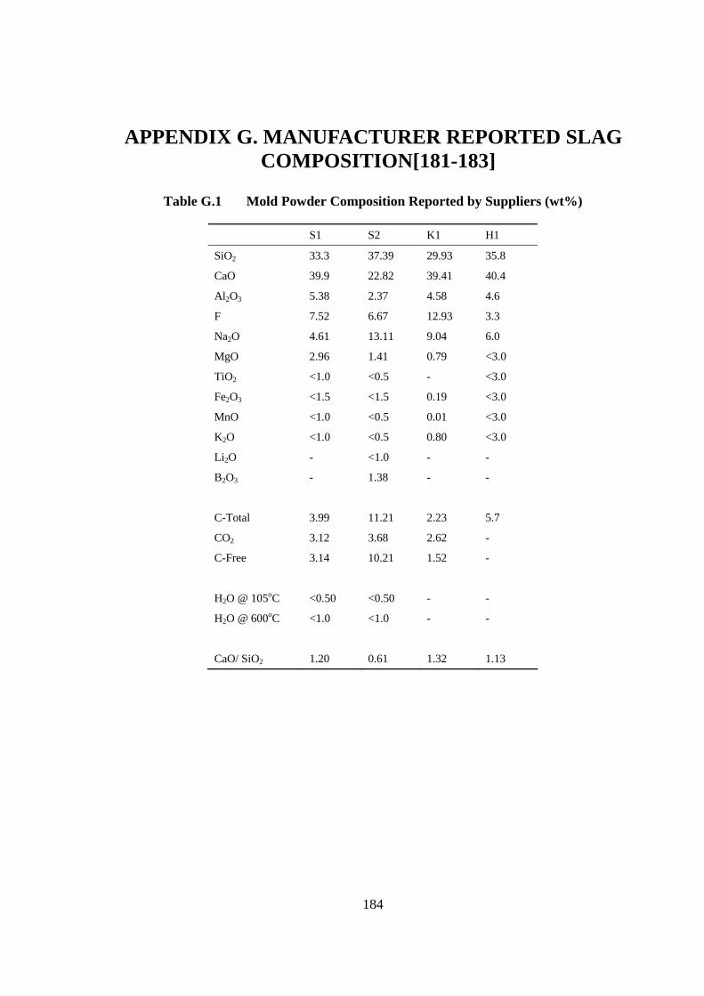
184

APPENDIX G. MANUFACTURER REPORTED SLAG COMPOSITION[181-183]

Table G.1 Mold Powder Composition Reported by Suppliers (wt%)

S1 S2 K1 H1

SiO2 33.3 37.39 29.93 35.8

CaO 39.9 22.82 39.41 40.4

Al2O3 5.38 2.37 4.58 4.6

F 7.52 6.67 12.93 3.3

Na2O 4.61 13.11 9.04 6.0

MgO 2.96 1.41 0.79 <3.0

TiO2 <1.0 <0.5 - <3.0

Fe2O3 <1.5 <1.5 0.19 <3.0

MnO <1.0 <0.5 0.01 <3.0

K2O <1.0 <0.5 0.80 <3.0

Li2O - <1.0 - -

B2O3 - 1.38 - -

C-Total 3.99 11.21 2.23 5.7

CO2 3.12 3.68 2.62 -

C-Free 3.14 10.21 1.52 -

H2O @ 105oC <0.50 <0.50 - -

H2O @ 600oC <1.0 <1.0 - -

CaO/ SiO2 1.20 0.61 1.32 1.13

185

APPENDIX H. AK STEEL BREAKOUT SHELL GROWTH

An analysis was performed by Stone et al to evaluate shell growth predictions by

CON1D against measurements obtained from the AK breakout shell[32, 105]. The

following table was used to convert the steady state results to transient shell growth

during breakout.

Table H.1 AK Steel Breakout Shell Drainage Time vs. Distance

Drainage Time (sec) Distance (mm)

0 0

1.1 19.84

2.4 33.06

3.3 45.18

4.5 59.51

5.8 70.53

6.7 83.75

7.7 96.98

8.7 109.1

9.4 122.32

9.9 127.84

16.4 254.69

22.2 378.77

28 509.39

33.5 633.47

39.9 764.08

45.8 894.69

52.1 1018.8

58.4 1142.9

64.9 1273.5

77.4 1449.8

186

APPENDIX I. CON1D VERSION 7.5 SAMPLE INPUT AND OUTPUT FILES

I.1 Input file: sample.inp

CON1D-7.5 Slab Casting Heat Transfer Analysis University of Illinois, Brian G. Thomas, 2002 Input Data INP (1) CASTING CONDITIONS: 1 Number of time-cast speed data points (If=1, constant casting speed) Next 2 lines contain time(s) and vc(m/min) data points 0. 1.000 1550.0 Pour temperature (C) 230.10 Slab thickness (mm) 1500.0 Slab width (mm) 94.000 Distance of meniscus from top of mold (mm) 800.00 Working mold length (mm) 20.000 Z-distance for heat balance (mm) 265.00 Nozzle submergence depth (mm) (2) SIMULATION PARAMETERS: 0 Which shell to consider? (0=wide face; 1=narrow face) 0 What type of mold? (0=slab, 1=funnel mold, 2=billet mold) 2 Which moldface to consider? (0=outer, 1=inner, 2=straight) 0 Calculate mold and interface (=0 flux casting, or 2 oil casting ) or enter interface heat flux data (=-1) 7 Number of zmm and q data points (if above = -1) Next 2 lines contain zmm(mm) and q(kW/m2) data 0. 100. 200. 300. 400. 600. 800. 2910. 1840. 1580. 1390. 1260. 1000. 880. 1.000 Is superheat treated as heatflux? 0=no; 1=yes (take default); -1=yes (enter data) 12 Number of zmm and q data points(if above = -1) Next 2 lines contain zmm(mm) and q(kW/m2) data 0. 100. 200. 260. 300. 500. 700. 1000. 1500. 2000. 3000. 10000. 94. 97. 92. 109. 197. 211. 12. 14. 80. 20. 0. 0. 1 Do you want (more accurate) 2d calculations in mold? (0=no; 1=yes; 2=yes, one extra loop for better taper) 800.00 Max. dist. below meniscus for 2d mold calcs (mm) (=mold length if above = 2) 2.00E-03 Time increment (s) 100 Number of slab sections 100.000 Printout interval (mm) 0. 00 Start output at (mm) 1500.0 Max. simulation length (must > z-distance)(mm) 50.000 Max. simulation thickness (mm) (smaller of max. expected shell thickness & half of slab thickness) 1000000 Max. number of iterations 3 Shell thermocouple numbers below hot face (less than 10) Next line gives the distance below surface of thermocouples(mm) 10.0 12.5 25.0 0.3000000 Fraction solid for shell thicknesss location (-) (3) STEEL PROPERTIES: 0.0500 1.520 0.015 0.012 0.340 %C,%Mn,%S,%P,%Si 0.0000 0.0000 0.0000 0.0000 0.0000 %Cr,%Ni,%Cu,%Mo,%Ti 0.0000 0.0000 0.0000 0.0000 0.0000 %Al,%V ,%N ,%Nb,%W 0.0000 %Co,(additional components) 1000 Grade flag

187

(1000,304,316,317,347,410,419,420,430,999) 1 If CK simple Seg. Model wanted for default Tliq,Tsol (1=yes,0=no) 10.00000 Cooling rate used in Seg.Model(if above =1) (K/sec) Override defaults with following constants(-1=default) -1.000000 Steel liquidus temperature (C) -1.000000 Steel solidus temperature (C) -1.000000 Steel density (g/cm^3) -1.000000 Heat fusion of steel (kJ/kg) -1.000000 Steel emissivity (-) -1.000000 Steel specific heat (kJ/kg deg K) -1.000000 Steel thermal conductivity (W/mK) -1.000000 Steel thermal expansion coeff. (/K) (4) SPRAY ZONE VARIABLES: 35.00000 Water and ambient temperature after spray zone(Deg C) spray zone condition:(heat tran.coeff.funct:h=A*C*W^n(1-bT)) (Nozaki Model:A*C=0.3925,n=0.55,b=0.0075) 1.570000 A(0=off) 0.5500000 n 0.0075 b 8.700000 minimum convection heat trans. coeff. (natural) (W/m^2K) 4 Number of zones No. zone rol. water spray contct frac.of spray conv amb. starts # rad. flowrate width length angle q thr rol coeff coeff temp. (mm) (m) (l/min/row) (m) (m) (Deg) (W/m^2K) (DegC) 1 800.0 1 0.075 18.882 0.984 0.904 0.00 0.010 0.250 8.70 25.0 2 2000.0 1 0.075 9.187 0.984 0.050 10.00 0.080 0.250 8.70 25.0 3 2710.0 1 0.095 5.195 0.984 0.050 10.00 0.220 0.250 8.70 25.0 4 8700.0 5 0.095 3.897 0.984 0.050 10.00 0.200 0.250 8.70 25.0 14000.0 End of last spray zone (mm) (5) MOLD FLUX PROPERTIES:(flux A2 in Ref #41 by Lanyi) 32.30 36.40 0.70 5.00 1.90 %CaO,%SiO2,%MgO,%Na2O,%K2O 3.00 0.00 0.00 0.00 0.00 %FeO,%Fe2O3,%NiO,%MnO,%Cr2O3 8.90 0.00 3.40 0.00 0.00 %Al2O3,%TiO2,%B2O3,%Li2O,%SrO 0.00 8.30 0.00 0.00 0.00 %ZrO2,%F,%free C,%total C,%CO2 950.0000 Mold flux solidification temperature(c) 1.500000 Solid flux conductivity(W/mK) 1.500000 Liquid flux conductivity(W/mK) 4.300000 Flux viscosity at 1300C (poise) 2500.000 Mold flux density(kg/m^3) 250.0000 Flux absorption coefficient(1/m) 1.500000 Flux index of refraction(-) (-1 = take default f(composition) 0.900000 Slag emissivity(-) 1.60000 Exponent for temperature dependency of viscosity 1 Form of mold powder consumption rate(1=kg/m^2; 2=kg/t) 0.411000 Mold powder consumption rate 0.0000E+00 Location of peak heat flux (m) 0.0000E+00 Slag rim thickness at metal level (meniscus) (mm) 0.0000E+00 Slag rim thickness at heat flux peak (mm) 10.00000 Liquid pool depth (mm) 8.0E+30 Solid flux tensile fracture strength (KPa) 8.0E+30 Solid flux compress fracture strength (KPa) 0.170000 Solid flux Poisson ratio(-) 0.400000 Max. Static friction coeff. between solid flux and mold wall 0.400000 Moving friction coefficient between solid flux and mold wall (6) INTERFACE HEAT TRANSFER VARIABLES: 1 Number of distance-vratio data points (1=constant ratio of solid flux velocity to casting speed) Next 2 lines contain zmm(mm) and ratio(-) data 0. 0.06 5.000E-09 Flux/mold or shell/mold contact resistance(m^2K/W) 0.5000000 Mold surface emissivity(-) 0.06 Air conductivity(W/mK) 0 Osc.marks simulation flag(0=average,1=transient)

188

0.450000 Oscillation mark depth(mm) 4.500000 Width of oscillation mark (mm) 1.388889 Oscillation frequency(cps) (-1=take default cpm=2*ipm casting speed) 7.800000 Oscillation stroke(mm) (7) MOLD WATER PROPERTIES: -1.000000 heat transfer coefficient(W/m^2K) (-1=default=f(T), based on Sleicher and Rouse Eqn) 4179.000 Water heat capacity(J/kgK)(-1=default=f(T)) 995.6000 Water density(kg/m3)(-1=default=f(T)) (8) MOLD GEOMETRY: 51.00000 WF Mold thickness with water channel (mm),(outer rad.,top) 51.00000 WF Mold thickness with water channel (mm),(inner rad.,top) 51.00000 Narrow face (NF) mold thickness with water channel (mm) 30.00000 Equivalent thickness of water box (mm) -1.000000 Mean temperature diff between hot & cold face of NF (C) 25.00000 25.00000 Cooling water channel depth(mm)(WF,NF) 5.000000 5.000000 Cooling water channel width(mm)(WF,NF) 29.00000 29.00000 Channel distance(center to center)(mm)(WF,NF) 7672.414 2200.000 Total channel cross sectional area(mm^2)(WF,NF) (served by water flow line where temp rise measured) 315.0000 315.0000 Mold thermal conductivity(W/mK)(WF,NF) 1.6000000E-05 Mold thermal expansion coeff. (1/K) 30.00000 Cooling water temperature at mold top(C) 0.2020000 Cooling water pressure(MPa) 1 Form of cooling water velocity/flowrate(1=m/s ; 2=L/s) 7.800000 7.800000 Cooling water velocity/flowrate per face (WF,NF) (> 0 cooling water from mold top to bottom < 0 cooling water from mold bottom to top) 0.0000000E+00 funnel height (mm) 0.0000000E+00 funnel width (mm) 0.0000000E+00 funnel depth at mold top (mm) 11.76000 Machine inner radius(m) 11.98500 Machine outer radius(m) 3 Number of mold coating/plating thickness changes down mold No. Scale Ni Cr Others Air gap Z-positions unit 1 0.010 1.000 0.100 0.000 0.000 0.000 (mm) 2 0.010 1.000 0.100 0.000 0.000 400.000 (mm) 3 0.010 1.000 0.100 0.000 0.000 800.000 (mm) 0.550 72.100 67.000 1.000 0.060 Conductivity (W/mK) (9) MOLD THERMOCOUPLES: 4 Total number of thermocouples No. Distance beneath Distance below hot surface(mm) meniscus(mm) 1 19.5 -1.00 2 19.5 20.00 3 19.5 121.00

4 19.5 226.00

I2 Output file: sample.ext

CON1D-7.5 Slab Casting Heat Transfer Analysis University of Illinois, Brian G. Thomas, 2002 EXIT Calculated Conditions EXT Initial casting speed: 16.67 (mm/s) Carbon content: 0.0500 (%) Wide face simulation: Steel Properties: The following 3 temperature from Y.M.Won Segregation Model

189

Liquidus Temp: 1532.10 Deg C Solidus Temp: 1515.31 Deg C Peritectic Temp: 0.00 Deg C AE3 Temp: 888.29 Deg C AE1 Temp: 723.00 Deg C Parameters Based on Derived Mold Values: Carbon equivalent: 0.0500 (%) (using initial casting speed:) Negative strip time: 0.24 (s) Positive strip time: 0.48 (s) Velocity amplitude of mold oscillation: 34.03 (mm/s) Pitch(spacing betweeen oscillation marks): 12.00 (mm) % Time negative strip: 33.71 (%) Average percent negative strip velocity: 30.00 (%) Cooling water velocity: 7.80 (m/s) Cooling water flow rate per face: 59.8448 (L/s) Average mold flux thickness: 0.0555 (mm) (based on consumption rate) (assuming flux moves at casting speed) min. heat trans. coeff. on mold cold face 14.72 kW/m2K max. heat trans. coeff. on mold cold face 19.30 kW/m2K Water boiling temperature: 120.528 Deg C Max cold face temperature: 161.765 Deg C Max hot face temperature(copper only): 361.551 Deg C Max hot face temperature(w/coating): 404.129 Deg C Mold water temp diff(in hot channel): 8.2918 Deg C Mold water temp diff(over all channels): 6.9875 Deg C *** Warning: There is danger of boiling in the water channels! Mean heat flux in mold: 1449.42 (kW/m^2) Friction Values: Average absolute shear stress in Mold: 7.7788 (kPa) Average friction force in Mold: 9.3346 (kN) Max. shear stress in Mold: 10.2271 (kPa) Max friction force in Mold: 12.2726 (kN) Min. shear stress in Mold: -7.6977 (kPa) Min friction force in Mold: -9.2372 (kN) shear stress in Mold when Vmold=0: 7.5690 (kPa) Friction force in Mold when Vmold=0: 9.0828 (kN) Calculated solid flux velocity ratio 0.0000 (-) Calculated solid flux consumption: 0.000E+00 (m^2) Used solid flux consumption: 0.787E-04 (m^2) Calculated liquid flux consumption: 0.213E-04 (m^2) Used liquid flux consumption: 0.494E-04 (m^2) Used osc. flux consumption: 0.135E-03 (m^2) Heat Balance at 20.00mm: Heat Extracted: 4.07 (MJ/m^2) Heat Input to shell inside: 0.12 (MJ/m^2) Super Heat: 0.01 (MJ/m^2) Latent Heat in mushy region: 0.77 (MJ/m^2) Latent Heat in Solid region: 2.51 (MJ/m^2) Sensible Cooling: 0.61 (MJ/m^2) Total Heat: 4.02 (MJ/m^2) Error In Heat Balance: 1.30 (%) Heat Balance at Mold Exit( 800.03mm): Heat Extracted: 69.58 (MJ/m^2) Heat Input to shell inside: 2.49 (MJ/m^2) Super Heat: 0.08 (MJ/m^2) Latent Heat in mushy region: 1.72 (MJ/m^2) Latent Heat in Solid region: 41.61 (MJ/m^2) Sensible Cooling: 24.75 (MJ/m^2) Total Heat: 70.64 (MJ/m^2) Error In Heat Balance: 1.53 (%)

190

Variables Calculated at Mold Exit( 800.03mm): taper (per mold, narrow face): 1.79 (%) taper (per mold per length, narrow face): 2.24 (%/m) Shell thickness: 22.37 (mm) Liquid flux film thickness: 0.0207 (mm) Solid flux film thickness: 1.2232 (mm) Total flux film thickness: 1.2439 (mm) Shell surface temperature: 1008.02 Deg C Mold hot face temperature: 179.78 Deg C Heat flux: 0.9445 (MW/m^2) Predicted Thermocouple Temperatures: No. distance beneath distance below temperature hot surface(mm) meniscus(mm) Deg C 1 19.50 -1.00 138.26 2 19.50 20.00 191.59 3 19.50 121.00 181.26 4 19.50 226.00 151.17

I3 Output file: sample.shl

# CON1D V7.5 Slab Casting Heat Transfer Analysis # University of Illinois, Brian G. Thomas, 2002 # SHELL Output Shell Temperature, Shrinkage Histories SHL # Posi time LiqLoc SolLoc shell Tsprime Surf EndWall Endwall # Temp Defl1 Defl2 # mm s mm mm mm C C mm mm # 0.00 0.0000 0.00 0.00 0.00 1532.6 1532.6 0.000 0.000 100.03 6.0019 6.50 5.39 5.98 1137.9 1231.0 6.436 7.575 200.01 11.9995 10.24 8.71 9.45 1074.1 1151.4 7.782 9.960 300.01 18.0000 13.01 11.34 12.25 1038.2 1106.3 8.540 11.411 …… 800.03 48.0049 23.50 20.97 22.37 960.3 1008.0 10.181 15.038 900.00 54.0016 25.00 22.49 23.95 1154.4 1164.6 7.559 14.723 1000.01 60.0003 26.50 23.79 25.43 1159.4 1179.6 7.307 14.587

I4 Output file: sample.mld

# CON1D V7.5 Slab Casting Heat Transfer Analysis # University of Illinois, Brian G. Thomas, 2002 # MOLD Mold Output MLD # Z Mold TSurf Mold Temp Heatflux qcold hwater hmold twater # thick hot hotcu cold # mm mm Deg C (Deg C) MW/m^2 MW/m2 W/m^2K W/m^2K Deg C # 0.0 26.0 1532.6 307.0 244.3 109.8 4.076 1.495 18743.6 6678.2 30.00 100.0 26.0 1231.0 349.4 317.9 147.7 2.049 2.064 17813.9 6491.9 31.87 200.0 26.0 1151.4 283.7 258.5 122.7 1.637 1.651 18433.3 6572.4 33.17 300.0 26.0 1106.3 248.3 226.6 109.9 1.412 1.418 18734.9 6610.3 34.25 …… 600.0 26.0 1035.0 197.6 181.1 92.8 1.069 1.071 19144.3 6660.6 36.86 700.0 26.0 1020.3 187.9 172.5 89.7 1.001 1.002 19225.7 6670.4 37.60 800.0 26.0 1008.0 179.8 165.3 87.8 0.944 0.955 19290.9 6678.2 38.29

191

I5 Output file: sample.gpt

# CON1D V7.5 Slab Casting Heat Transfer Analysis # University of Illinois, Brian G. Thomas, 2002 # GAPT Output Heat Transfer,Powder Layer Thicknesses Histories GPT # Z-dist hrad hcond dsolid dliquid deff dtotal visc # (mm) W/m^2K W/m^2K (mm) (mm) (mm) (mm) Poise # 0.0 1302.8 5693.7 0.237 0.212 0.052 0.448 0.218E+01 100.0 930.3 6359.5 0.440 0.168 0.068 0.607 0.116E+02 200.0 850.5 7276.7 0.611 0.135 0.071 0.746 0.226E+02 300.0 808.5 8224.9 0.745 0.110 0.072 0.855 0.390E+02 …… 600.0 747.6 11829.2 1.056 0.052 0.075 1.108 0.201E+03 700.0 736.0 13495.0 1.142 0.036 0.075 1.178 0.418E+03 800.0 726.5 15551.8 1.223 0.021 0.076 1.244 0.121E+04

I6 Output file: sample.gpv

# CON1D V7.5 Slab Casting Heat Transfer Analysis # University of Illinois, Brian G. Thomas, 2002 # GAPV Output Powder Layer Consumption and Velocities GPV # Z-dist qconsumpt qosciltn qliquid qsolid vliquid vsolid # mm m^2/s m^2/s m^2/s m^2/s m/s m/s # 0. 0.2740E-05 0.141E-05 0.110E-05 0.237E-06 0.519E-02 0.100E-02 100. 0.2740E-05 0.141E-05 0.894E-06 0.440E-06 0.533E-02 0.100E-02 200. 0.2740E-05 0.141E-05 0.723E-06 0.611E-06 0.535E-02 0.100E-02 300. 0.2740E-05 0.141E-05 0.588E-06 0.745E-06 0.535E-02 0.100E-02 …… 600. 0.2740E-05 0.141E-05 0.278E-06 0.106E-05 0.535E-02 0.100E-02 700. 0.2740E-05 0.141E-05 0.191E-06 0.114E-05 0.535E-02 0.100E-02

I7 Output file: sample.spr

# CON1D V7.5 Slab Casting Heat Transfer Analysis # University of Illinois, Brian G. Thomas, 2002 # SPRAY Output Heat Transfer History in Spray Zones below Mold SPR # Z-dist hnconv hrad hspray hconv2 htot # (mm) W/m^2K W/m^2K W/m^2K W/m^2K W/m^2K # 900.0 8.7 169.7 0.0 0.00 178.40 1000.0 8.7 176.1 163.5 0.00 348.24 1100.0 8.7 178.5 163.5 0.00 350.65 1200.0 8.7 180.1 163.5 0.00 352.24 1300.0 8.7 180.8 163.5 0.00 352.94 1400.0 8.7 180.9 163.5 0.00 353.02 1500.0 8.7 180.5 163.5 0.00 352.67

192

I8 Output file: sample.prf

# CON1D V7.5 Slab Casting Heat Transfer Analysis # University of Illinois, Brian G. Thomas, 2002 # PROFILE Temperature distribution and heat balance at mold exit PRF # Distance Temperature Super Heat Sensible Heat Latent Heat # mm Deg C kJ/m2 kJ/m2 kJ/m2 # 0.0000 1008.0 0.6 602.8 501.4 0.2500 1023.7 1.2 1174.0 1002.7 0.7500 1039.2 1.2 1142.4 1002.7 1.2500 1054.6 1.2 1110.8 1002.7 …… 48.7500 1532.6 0.0 0.0 0.0 49.2500 1532.6 0.0 0.0 0.0 49.7500 1532.6 0.0 0.0 0.0

I9 Output file: sample.shr

# CON1D V7.5 Slab Casting Heat Transfer Analysis # University of Illinois, Brian G. Thomas, 2002 # Shear Shear Stress in Gap SHR # Z-dist up axial dn axial max min Trans Avg Node1 Node9 Node17 # mm Pa Pa Pa Pa Pa Pa Pa Pa Pa # 0.000 -0.5018E+02 -0.5018E+02 0.1286E+03 -0.5391E+02 0.0 58.7 97.6 33.8 -57.4 100.032 -0.6134E+03 -0.1536E+04 0.9088E+03 -0.3191E+03 0.0 449.5 902.3 288.3 -325.7 200.014 -0.2098E+04 -0.3020E+04 0.2197E+04 -0.7589E+03 0.0 1087.4 2188.0 710.0 -768.0 300.015 -0.3584E+04 -0.4506E+04 0.4676E+04 -0.1607E+04 0.0 2316.2 4665.2 1523.6 -1618.0 …… 600.008 0.1894E+07 -0.8963E+04 0.5104E+05 -0.1749E+05 0.0 14088.2 17502.0 16760.8 -17501.0 700.017 0.8386E+07 -0.1104E+07 0.1540E+06 -0.5275E+05 0.0 19012.9 20402.8 20402.8 -20402.8 800.026 0.3665E+08 -0.9577E+07 0.7750E+06 -0.2655E+06 0.0 23304.0 23304.0 23304.0 -23304.0 # friction force in mold (N) # 800.03 76602.08 -26245.11 9334.9 12272.7 9083.1 -9237.5

I10 Output file: sample.tpr

# CON1D V7.5 Slab Casting Heat Transfer Analysis # University of Illinois, Brian G. Thomas, 2002 # Taper Output Taper Histories TPR # Posi EndWall Endwall WF NF Mold Extra IdealTpr IdealTpr IdealTpr # Defl-1s Defl-2 Expn Dstr Dstr Length Def Inst Cumul # mm mm mm mm mm mm mm mm %/m %/m # 0.00 0.000 0.000 -1.172 -2.343 -1.172 0.000 0.000 0.000 0.000 100.03 6.436 7.575 -2.794 -5.588 -2.794 0.000 7.867 3.244 10.487 200.01 7.782 9.960 -2.287 -4.575 -2.287 0.000 9.608 2.254 6.405 300.01 8.540 11.411 -2.019 -4.039 -2.019 0.000 10.681 0.988 4.747 …… 600.01 9.732 13.960 -1.644 -3.287 -1.644 0.000 12.602 0.569 2.800 700.02 9.976 14.539 -1.574 -3.147 -1.574 0.000 13.041 0.652 2.484 800.03 10.181 15.038 -1.518 -3.037 -1.518 0.000 13.418 0.534 2.236

193

I11 Output file: sample.frc

# CON1D V7.5 Slab Casting Heat Transfer Analysis # University of Illinois, Brian G. Thomas, 2002 # FRACTI Output phase fractions:L,delta,gamma,alpha FRC # Posi 10.00mm below surface | shell surface # mm Temp C Liquid Delta Gamma Alpha| Temp C Liquid Delta Gamma Alpha # 0. 1532.6 1.000 0.000 0.000 0.000 1532.6 1.000 0.000 0.000 0.000 100. 1532.3 1.000 0.000 0.000 0.000 1231.0 0.000 0.000 1.000 0.000 200. 1532.1 1.000 0.000 0.000 0.000 1151.4 0.000 0.000 1.000 0.000 300. 1486.4 0.000 1.000 0.000 0.000 1106.3 0.000 0.000 1.000 0.000 …… 800. 1296.6 0.000 0.000 1.000 0.000 1008.0 0.000 0.000 1.000 0.000 900. 1300.1 0.000 0.000 1.000 0.000 1164.6 0.000 0.000 1.000 0.000 1000. 1318.1 0.000 0.000 1.000 0.000 1179.6 0.000 0.000 1.000 0.000

I12 Output file: sample.fxt

# CON1D V7.5 Slab Casting Heat Transfer Analysis # University of Illinois, Brian G. Thomas, 2002 # FLUX Flux temperature Output FXT # Delta x=0.2mm # Z t1 T1 t2 T2 t3 T3 t4 T4 t9 Tsurf # mm s C s C s C s C s C # 100.03 100.03 622.6 56.97 895.8 6.02 1129.7 6.00 0.0 6.00 1231.0 200.01 200.01 501.9 156.94 720.2 51.59 938.4 12.00 0.0 12.00 1151.4 300.01 300.01 436.6 256.96 624.8 151.59 813.1 21.91 993.7 18.00 1106.3 …… 600.01 600.01 340.1 556.95 482.6 451.63 625.2 307.19 767.7 36.01 1035.0 700.02 700.02 321.3 656.96 454.8 551.64 588.2 407.20 721.6 42.01 1020.3 800.03 800.03 305.7 756.97 431.6 651.65 557.6 507.21 683.5 48.00 1008.0

I13 Output file: sample.sst

# CON1D V7.5 Slab Casting Heat Transfer Analysis # University of Illinois, Brian G. Thomas, 2002 # Shell Outpput Steel Shell Temperature Below Surface SST # Posi Surf 1 2 3 4 5 6 7 8 9 10 # mm C C C C C C C C C C C # 0.00 10.00 12.50 25.00 0.00 0.00 0.00 0.00 0.00 0.00 0.00 0.0 1532.6 1532.6 1532.6 1532.6 0.0 0.0 0.0 0.0 0.0 0.0 0.0 100.0 1231.0 1532.3 1532.4 1532.6 0.0 0.0 0.0 0.0 0.0 0.0 0.0 200.0 1151.4 1532.1 1532.3 1532.6 0.0 0.0 0.0 0.0 0.0 0.0 0.0 300.0 1106.3 1486.4 1532.0 1532.6 0.0 0.0 0.0 0.0 0.0 0.0 0.0 …… 800.0 1008.0 1296.6 1355.5 1532.2 0.0 0.0 0.0 0.0 0.0 0.0 0.0 900.0 1164.6 1300.1 1346.0 1532.1 0.0 0.0 0.0 0.0 0.0 0.0 0.0 1000.0 1179.6 1318.1 1355.1 1529.9 0.0 0.0 0.0 0.0 0.0 0.0 0.0

194

I14 Output file: sample.sst

# CON1D V7.5 Slab Casting Heat Transfer Analysis # University of Illinois, Brian G. Thomas, 2002 #SEGREGATION Segr. Related Params. vs Dist. below Shell Surface SEG # Information only (not used in CON1D calculation) # Distance tf CR SDAS Tsol # mm sec K/sec um C 0.0000 0.1500 111.9019 12.9697 1515.3097 0.2500 0.4180 40.1561 21.5070 1515.3119 0.7500 0.6520 25.7444 26.7830 1515.3129 1.2500 0.6960 24.1171 27.6601 1515.3130 …… 22.2500 9.7107 1.7285 101.5632 1515.3182 22.7500 10.2224 1.6420 104.1701 1515.3184 23.2500 10.8900 1.5413 107.4738 1515.3185 # At 1000.04mm below meniscus, liquid still exists from 23.75mm below shell surface

I15 Output file: sample.liq

# CON1D V7.5 Slab Casting Heat Transfer Analysis # University of Illinois, Brian G. Thomas, 2002 # Liquid Phase Concentration Output LIQ # Information only (not used in CON1D calculation) # Position: surface # Z time Temp fl C% Si% Mn% P% S% # mm sec Deg C 0.5 0.03 1519.49 0.787 0.0604 0.3582 1.6059 0.0144 0.0188 1.0 0.06 1517.24 0.578 0.0760 0.3798 1.7104 0.0180 0.0251 1.5 0.09 1513.70 0.371 0.1020 0.4063 1.8436 0.0241 0.0374 2.0 0.12 1508.45 0.203 0.1412 0.4332 1.9857 0.0337 0.0625 2.5 0.15 1499.80 0.073 0.2012 0.4589 2.1287 0.0497 0.1307 3.0 0.18 1486.54 0.002 0.2620 0.4753 2.2250 0.0680 0.3258 # From 3.5mm below meniscus only solid phase exists

I16 Output file: sample.sol

# CON1D V7.5 Slab Casting Heat Transfer Analysis # University of Illinois, Brian G. Thomas, 2002 # Solid Phase Concentration Output SOL # Information only (not used in CON1D calculation) # Position: surface # Z time Temp fs fd fg C% Si% Mn% P% S% # mm sec Deg C 0.5 0.03 1519.49 0.213 0.213 0.000 0.0115 0.2758 1.2204 0.0033 0.0009 1.0 0.06 1517.24 0.422 0.422 0.000 0.0144 0.2924 1.2999 0.0041 0.0013 1.5 0.09 1513.70 0.629 0.629 0.000 0.0194 0.3128 1.4011 0.0055 0.0019 2.0 0.12 1508.45 0.797 0.797 0.000 0.0268 0.3336 1.5091 0.0077 0.0031 2.5 0.15 1499.80 0.927 0.927 0.000 0.0382 0.3533 1.6178 0.0114 0.0065 3.0 0.18 1486.54 0.998 0.998 0.000 0.0498 0.3660 1.6910 0.0157 0.0163 # From 3.5mm below meniscus only solid phase exists

195

REFERENCES

1. Irving, W.R.: Continuous Casting of Steel, The Institute of Materials, London, 1993.

2. "World Steel in Figures", World Steel in Figures, International Iron and Steel Institute, 2003

3. Tanner, A.H.: Continuous Casting: A Revolution in Steel, Write Stuff Enterprises, INC., 1998.

4. Huang, X. and Thomas, B.G.: "Modeling of Steel Grade Transition in Continuous Slab Casting Processes", Metallurgical Transactions B (USA), 1993, vol. 24B (2), pp. 379-393.

5. Wolf, M.M.: "Mold Heat Transfer and Lubrication Control Two Major Functions of Caster Productivity and Quality Assurance", Continuous Casting 1997, vol. Volume 9: Initial Solidification and Strand Surface Quality of Peritectic Steels, ISS/AIME, Warrendale, PA, pp. 211-222, 1997

6. Pinheiro, C.A., Samarasekera, I.V. and Brimacombe, J.K.: "Mold Flux for Continuous Casting of Steel Part Xv: Heat Transfer", Iron and Steelmaker (USA), 1995, vol. 22 (12), pp. 43-44.

7. Billany, T.J.H., Normanton, A.S., Mills, K.C. and Grieveson, P.: "Surface Cracking in Continuously Cast Producs", Ironing and Steelmaking, 1991, vol. 18 (6), pp. 403-410.

8. Meng, Y. and Thomas, B.G.: "Heat Transfer and Solidification Model of Continuous Slab Casting: Con1d", Metall. Mater. Trans. B (USA), 2003, vol. 34B (5), pp. 685-705.

9. Najjar, F.M., Thomas, B.G. and Hershey, D.E.: "Numerical Study of Steady Turbulent Flow through Bifurcated Nozzles in Continuous Casting", Metall. Mater. Trans. B (USA), 1995, vol. 26B (4), pp. 749-765.

10. Kubrik, B.I.: "Effects of Thermal and Physical Properties of Slag and Coefficients of Thermal Conductivity of Mould Walls on Heat Transfer in Mould", Steel USSR, 1987, vol. 17 (12), pp. 573-575.

11. Machingawuta, N.C., Bagha, S. and Grieveson, P.: "Heat Transfer Simulation for Continuous Casting", Steelmaking Conference Proceedings, (Washington, D.C., USA, 14-17 Apr. 1991), ISS, Warrendale, PA, 1991, pp. 163-170.

12. Cimarelli, T.: "Mould Powder Influence on Continuous Casting Operations and on Slabs Surface Quality", Metallurgia Italiana (Italy), 1997, vol. 89 (9), pp. 31-37.

13. Takeuchi, E. and Brimacombe, J.K.: "The Formation of Oscillation Marks in the Continuous Casting of Steel Slabs", Metall. Trans. B, 1984, vol. 15B (3), pp. 493-509.

196

14. Pinheiro, C.A., Samarasekera, I.V. and Brimacombe, J.K.: "Mold Flux for Continuous Casting of Steel Part Xvii Mold Flux Related Defects", Iron and Steelmaker (USA), 1996, vol. 23 (2), pp. 59-60.

15. Suzuki, M., Mizukami, H., Kitagawa, T., Kawakami, K., Uchida, S. and Komatsu, Y.: "Development of a New Mold Oscillation Mode for High-Speed Cc of Steel Slabs", ISIJ International (Japan), 1991, vol. 31 (3), pp. 254-261.

16. Nakamori, Y., Fujikake, Y. and Tokiwa, K.: "Development of Friction Measuring System in a Continuous Casting Mold", Tetsu-to-Hagane (J. Iron Steel Inst. Jpn.), 1984, vol. 70 (9), pp. 1262-1268.

17. DiLellio, J.A. and Young, G.W.: "Asymptotic Model of the Mold Region in a Continuous Steel Caster", Metallurgical and Materials Transactions B: Process Metallurgy and Materials Processing Science, 1995, vol. 26B (6), pp. 1225-1441.

18. Wolf, M.M.: "Review of Mould Fricrtion", BHM, 2000, vol. 145 (7), pp. 270-275.

19. Lawson, G.D., Sander, S.C., Emling, W.H., Moritra, A. and Thomas, B.G.: "Prevention of Shell Thinning Breakouts Associated with Widening Width Changes", 77th Steelmaking Conference, (Chicago, IL, USA, 20-23 Mar. 1994), ISS/AIME, Warrendale, PA, 1994, pp. 329-336.

20. Thomas, B.G., Moitra, A. and McDavid, R.: "Simulation of Longitudinal Off-Corner Depressions in Continuously Cast Steel Slabs", Iron and Steelmaker (USA), 1996, vol. 23 (4), pp. 57-70.

21. Thomas, B.G. and Ojeda, C.: "Ideal Taper Prediction for Slab Casting", ISSTech Steelmaking Conference, (Indianapolis, IN, USA, April 27-30, 2003), 2003, pp. 396-308.

22. Tony, W.A.: "Small Ticket Item Proving to Have Big Impact", Iron and Steelmaker (USA), 1992, vol. 19 (4), pp. 17-20.

23. Mills, K.C.: "The Performance of Casting Powders", Steel Technol. Int., 1994, pp. 161-166.

24. Nakato, H., Takeuchi, S., Fujii, T., Nozaki, T. and Washio, M.: "Characteristics of New Mold Fluxes for Strand Casting of Low and Ultra Low Carbon Steel Slabs", Steelmaking Conference Proceedings, (Washington, D.C., USA, 14-17 Apr. 1991), 1991, pp. 639-646.

25. Moore, J.A., Phillips, R.J. and Gibbs, T.R.: "An Overview for the Requirements of Continuous Casting Mold Fluxes", Steelmaking Conference Proceedings, (Washington, D.C., USA, 14-17 Apr. 1991), 1991, pp. 615-621.

26. Pinheiro, C.A., Samarasekera, I.V. and Brimacombe, J.K.: "Mold Flux for Continuous Casting of Steel Part V: Crystallization Temperature", I&SM, 1995, vol. 22 (2), pp. 37-39.

27. Bhamra, M.S., Charlesworth, M.G., Wong, S., Sawyers-Villers, D. and Cramb, A.W.: "Crystallization of Fluxes under Varying Cooling Rates", 54th Electric Furnace Conference, (Dallas, Texas, USA, 9-12 Dec. 1996), ISS/AIME, Warrendale, PA, 1996, pp. 551-564.

197

28. Orrling, C., Cramb, A.W., Tilliander, A. and Kashiwaya, Y.: "Observations of the Melting and Solidification Behavior of Mold Slags", Iron and Steelmaker (USA), 2000, vol. 27 (1), pp. 53-63.

29. O'Malley, R.J.: "Observations of Various Steady State and Dynamic Thermal Behaviors in a Continuous Casting Mold", 82nd Steelmaking Conference, (Chicago, IL, USA, 21-24 Mar. 1999), ISS/AIME, Warrendale, PA, 1999, pp. 13-33.

30. Thomas, B.G., Ho, B. and Li, G.: "Heat Flow Model of the Continuous Slab Casting Mold, Interface, and Shell", Alex McLean Symposium: Process Fundamentals, Liquid Metal Processing for Cleanliness, Novel and Conventional Casting, and Novel Process Technologies, (Toronto, Ontario, Canada, 12-14 July 1998), Iron and Steel Society/AIME, Alex McLean Symposium Proceedings (USA), 1998, pp. 177-193.

31. Ho, B.: Characterization of Interfacial Heat Transfer in the Continuous Slab Casting Process, Master Thesis, UIUC, 1992.

32. Stone, D.T.: Mathematical Modeling of Interfacial Heat Transfer in the Continuous Slab Casting Process, M.S. Thesis, University of Illinois, Champaign-Urbana, 2000.

33. Nakato, H., Omiya, S., Habu, Y., Hamagami, K. and Koshikawa, T.: "Optimizing Mold Lubrication for High-Speed Continuous Casting of Slabs", Journal of metals, 1984, vol. 36 (3), pp. 44-50.

34. Thomas, B.G., O'malley, R.J., Shi, T., Meng, Y., Creech, D. and Stone, D.: "Validation of Fluid Flow and Solidification Simulation of a Continuous Thin-Slab Caster", Modeling of Casting, Welding and Advanced Solidification Process IX, (Aachen, Germany, Aug. 20-25, 2000), TMS, Warrendale, PA, 2000, pp. 769-776.

35. Thomas, B.G. and Morthland, T.: 3-D Heat Transfer Analysis of Columbus Slab Casting Mold, Columbus Steel, Urbana, IL, 2001.

36. Park, J.K., Thomas, B.G. and Samarasekera, I.V.: "Analysis of Thermo-Mechnical Behavior in Billet Casting with Different Mold Cornerradii", ironmaking and Steelmaking, 2002, vol. 29 (5), pp. 359-375.

37. Lin, K.J. and Thomas, B.G.: "Thermal Stress Analysis of Bulging with Roll Misalignment for Various Slab Cooling Intensities", China Steel Technical Report (Taiwan), 2002, vol. 16 (Dec.), pp. 9-14.

38. Thomas, B.G.: "Mathematical Modeling of the Continuous Slab Casting Mold: A State of the Art Review", 1991 Steelmaking Conference, ISS, Warrendale, PA, 1991, pp. 69-82.

39. Thomas, B.G.: "Modeling of the Continuous Casting of Steel - Past, Present and Future", Metall. Mater. Trans. B (USA), 2002, vol. 33B (6), pp. 795-812.

198

40. Thomas, B.G. and Zhang, L.: "Mathematical Modeling of Fluid Flow in Continuous Casting", ISIJ International (Japan), 2001, vol. 41 (10), pp. 1181-1193.

41. Hills, A.W.D.: "A Generlized Intergral-Profile Method for the Analysis of Unidirectional Heat Flow During Solidification", Transactions TMS-AIME, 1969, vol. 245, pp. 1471-1479.

42. Mizikar, E.A.: "Mathematical Heat Transfer Model for Solidification of Continuosly Cast Steel Slabs", AIME MET SOC TRANS, 1967, vol. 239 (11), pp. 1747-1758.

43. Lait, J.E., Brimacombe, J.K. and Weinberg, F.: "Mathematical Modelling of Heat Flow in the Continuous Casting of Steel", ironmaking and Steelmaking, 1974, vol. 1 (2), pp. 90-97.

44. Grill, A., Sorimachi, K. and Brimacombe, J.K.: "Heat Flow, Gap Formation and Break-Outs in the Continuous Casting of Steel Slabs", Metall. Trans. B, 1976, vol. 7B (2), pp. 177-189.

45. Upton, E.A., Rao, T.R.S., Dauby, P.H. and Knechtges, R.C.: "Physical Metallurgy and Mathematical Modeling as Tools for Continuous Casting Optimization at Ltv Steel", Iron Steelmaker, 1988, vol. 15 (5), pp. 51-57.

46. Davies, R., Blake, N. and Campbell, P.: "Solidification Modelling--an Aid to Continuous Casting", 4th International Conference Continuous Casting. Preprints. Vol. 2, (Brussels, Belgium, 17-19 May 1988), Verlag Stahleisen, P.O. Box 8229, D-4000, Dusseldorf 1, FRG, 1988, pp. 645-654.

47. Mahapatra, R.B., Brimacombe, J.K. and Samarasekera, I.V.: "Mold Behavior and Its Influence on Quality in the Continuous Casting of Steel Slabs. Ii. Mold Heat Transfer, Mold Flux Behavior, Formation of Oscillation Marks, Longitudinal Off-Corner Depressions, and Subsurface Cracks", Metall. Trans. B, 1991, vol. 22B (6), pp. 875-888.

48. Brimacombe, J.K.: "Design of Continuous Casting Machine Based on a Heat Flow Analysis: State-of-the-Art Review", Canadian Metallurgical Quarterly, 1976, vol. 15 (2), pp. 163-175.

49. Kristiansson, J.O.: "Thermomechanical Behavior of the Solidifying Shell within Continuous-Casting Billet Molds - a Numerical Approach", Journal of Thermal Stresses, 1984, vol. 7, pp. 209-226.

50. Moitra, A. and Thomas, B.G.: "Application of a Thermo-Mechanical Finite Element Model of Steel Shell Behavior in the Continuous Slab Casting Mold", 76th Steelmaking Conference, (Dallas, TX, 28-31 Mar. 1993), ISS, Warrendale, PA, 1993, pp. 657-667.

51. Aboutalebi, M.R., Guthrie, R.I.L. and Hasan, M.: "Thermal Modelling and Stress Analysis in the Continuous Casting of Arbitrary Sections", Steel Research, 1994, vol. 65 (6), pp. 225-233.

199

52. Wimmer, F., Thone, H. and Lindorfer, B.: "Thermomechanically-Coupled Analysis of the Steel Solidification Process in the Continuous Casting Mold as a Basis for the Development of a High Speed Casting Mold", Berg- und Huttenmannische Monatshefte (Austria), 1996, vol. 141 (5), pp. 185-191.

53. Nam, H., Park, H.S. and Yoon, J.K.: "Numerical Analysis of Fluid Flow and Heat Transfer in the Funnel Type Mold of a Thin Slab Caster", ISIJ International (Japan), 2000, vol. 40 (9), pp. 886-892.

54. Choudhary, S.K. and Mazumdar, D.: "Mathematical Modelling of Transport Phenomena in Continuous Casting of Steel", ISIJ International (Japan), 1994, vol. 34 (7), pp. 584-592.

55. Lee, J.E., Yeo, T.J., Oh, K.H., Yoon, J.K. and Yoon, U.S.: "Prediction of Cracks in Continuously Cast Steel Beam Blank through Fully Coupled Analysis of Fluid Flow, Heat Transfer, and Deformation Behavior of a Solidifying Shell", Metallurgical and Materials Transactions A (USA), 2000, vol. 31A (1), pp. 225-237A.

56. Ohler, C., Odenthal, H.J., Pfeifer, H. and Lemanowicz, I.: "Numerical Simulation of the Fluid Flow and Solidification Phenomena in a Thin Slab Caster", Stahl und Eisen (Germany), 2002, vol. 122 (3), pp. 55-63.

57. Flint, P.: "A Three-Dimensional Finite Difference Model of Heat Transfer Fluid Flow and Solidification in the Continuous Slab Caster", Procedings of 73rd Steel Making Conference, (Detroit, ISS/AIME, Warrendale, PA, 1990, pp. 481-490.

58. Thomas, B.G., Storkman, W.R. and Moitra, A.: "Optimizing Taper in Continuous Slab Casting Molds Using Mathematical Models", IISC. The Sixth International Iron and Steel Congress, (Nagoya, Japan, Oct 21-26, 1990), ISIJ, Tokyo, Japan, 1990, pp. 348-355.

59. Li, C. and Thomas, B.G.: "Analysis of the Potential Productivity of Continuous Cast Molds", The Brimacombe Memorial Symposium, (Vancouver, British Columbia, Canada, 1-4 Oct. 2000), Canadian Institute of Mining, Metallurgy and Petroleum, Montreal PQ, Canada, 2000, pp. 595-611.

60. Laitinen, E. and Neittaanmaki, P.: "On Numerical Simulation of the Continuous Casting Process", Journal of Engineering Mathmatics, 1988, vol. 22, pp. 335-354.

61. Huang, X., Thomas, B.G. and Najjar, F.M.: "Modeling Superheat Removal During Continuous Casting of Steel Slabs", Metall. Mater. Trans. B (USA), 1992, vol. 23B (6), pp. 339-356.

62. Birat, J.P., Larrecq, M., Lamant, J.Y. and Petegnief, J.: "The Continuous Casting Mold: A Basic Tool for Surface Quality and Strand Productivity", 1991 Steelmaking Conference1991), 1991, pp. 3-14.

63. Samarasekera, I.V. and Brimacombe, J.K.: "Thermal and Mechanical Behavior of Continous-Casting Billet Molds", ironmaking and Steelmaking, 1982, vol. 9 (1), pp. 1-15.

200

64. Thomas, B.G., Li, G., Moitra, A. and Habing, D.: "Analysis of Thermal and Mechanical Behavior of Copper Molds During Continuous Casting of Steel Slabs", 80th Steelmaking Conference, (Chicago, IL, Iron and Steel Society, 1997, pp. 183-201.

65. Park, J.K., Samarasekera, I.V., Thomas, B.G. and Yoon, U.S.: "Analysis of Thermal and Mechanical Behavior of Copper Mould During Thin Slab Casting", 83rd Steelmaking Conference, (Pittsburgh, PA, USA, 26-29 Mar. 2000), ISS/AIME, Warrendale, PA, 2000, pp. 9-21.

66. Mahapatra, R.B., Brimacombe, J.K., Samarasekera, I.V., Walker, N., Paterson, E.A. and Young, J.D.: "Mold Behavior and Its Influence on Quality in the Continuous Casting of Steel Slabs. I. Industrial Trials, Mold Temperature Measurements, and Mathematical Modeling", Metall. Trans. B, 1991, vol. 22B (6), pp. 861-874.

67. Pinheiro, C.A.M., Samarasekera, I.V. and Walker, B.N.: "Mould Heat Transfer and Continously Cast Billet Quality with Mould Flux Lubrication Part 1: Mould Heat Transfer", Ironmaking and Steelmaking (UK), 2000, vol. 27 (1), pp. 37-54.

68. Samarasekera, I.V. and Brimacombe, J.K.: "The Thermal Field in Continuous-Casting Moulds", Canadian Metallurgical Quarterly, 1979, vol. 18, pp. 251-266.

69. Gilles, H.L., Byrne, M., Russo, T.J. and DeMasi, G.A.: "The Use of an Instrumented Mold in the Development of High Speed Slab Casting", Process Technology Conference Proceedings. Vol. 9. Use of Instrumentation to Optimize the Continuous Casting Process, (Detroit, Michigan, USA, 25-28 Mar. 1990), Iron and Steel Society, 1990, pp. 123-138.

70. Kapaj, N., Pavlicevic, M. and Poloni, A.: "Exceeding the Casting Speed of Bloom Cc Machines by Three Times", Steelmaking Conference, (Baltimore, Maryland USA, March 25-28, 2001), 2001, pp. 67-78.

71. Li, C.: Thermal-Mechanical Model of Solifying Steel Shell Behavior and Its Application in High Speed Continuous Casting of Billets, Ph.D Thesis, University of Illinois, Urbana-Champaign, 2004.

72. Wolf, M.M.: "Mold Length in Slab Casting--a Review", Iron and Steelmaker (USA), 1996, vol. 23, pp. 47-51.

73. Dippenaar, R.J., Samarasekera, I.V. and Brimacombe, J.K.: "Mold Taper in Continuous Casting Billet Machines", ISS Transactions, 1986, (7), pp. 331-343.

74. Chandra, S., Brimacombe, J.K. and Samarasekera, I.V.: "Mould-Strand Interaction in Continuous Casting of Steel Billets. Iii. Mould Heat Transfer and Taper", Ironmaking and Steelmaking (UK), 1993, vol. 20 (2), pp. 104-112.

75. Park, J.K., Thomas, B.G., Samarasekera, I.V. and Yoon, U.S.: "Thermal and Mechanical Behavior of Copper Molds During Thin-Slab Casting. Ii. Mold Crack Formation", Metall. Mater. Trans. B (USA), 2002, vol. 33b (3), pp. 437-449B.

201

76. Samarasekera, I.V., Anderson, D.L. and Brimacombe, J.K.: "The Thermal Distortion of Continuous Casting Billet Molds", Metall. Mater. Trans. B (USA), 1982, vol. 13 (March), pp. 91-104.

77. Wimmer, F., Thone, H. and Lindorfer, B.: "Thermomechanically-Coupled Analysis of the Steel Solidification Process as a Basis for the Development of a High Speed Billet Casting Mold", The International Conference on Modelling and Simulation in Metallurgical Engineering and Materials Science, (Beijing, China, 11-13, June 1996), Metallurgical Industry Press, Beijing, China, 1996, pp. 366-371.

78. Tiedje, N. and Langer, E.W.: "Metallographic Examination of Breakouts from a Continuous Billet Caster", Scandinavian Journal of Metallurgy (Denmark), 1992, vol. 21 (5), pp. 211-217.

79. Bagha, S., Machingawuta, N.C. and Grieveson, P.: "Heat Transfer Simulation for Continuous Casting", 3rd International Conference on Molten Slags and Fluxes, (Glasgow, UK, June 27-29, 1988), The Institute of Metals, 1 Carlton House Terrace, London SW1Y 5DB, UK, 1989, pp. 235-240.

80. Ohmiya, S., Tacke, K.H. and Schwerdtfeger, K.: "Heat Transfer through Layers of Casting Fluxes", ironmaking and Steelmaking, 1983, vol. 10 (1), pp. 24-30.

81. Ridolfi, M.R., Thomas, B.G., Li, G. and Foglia, U.D.: "The Optimization of Mold Taper for the Ilva-Dalmine Round Bloom Caster", Rev. Metall., Cah. Inf. Tech. (France), 1994, vol. 91 (4), pp. 609-620.

82. Jenkins, M.S.: "Characterization of Heat Transfer in a Continuous Casting Mold", Continuous Casting, vol. 9, Initial Solidification and Strand Surface Quality of Peritectic Steels (USA), Iron and Steel Society/AIME, pp. 239-244, 1997

83. Riboud, P.V. and Larrecq, M.: "Lubrication and Heat Transfer in a Continuous Casting Mold", Steelmaking Proceedings, (Detroit, Mich., USA, TMS/AIME, 1979, pp. 78-92.

84. Kor, G.J.W.: "An Analysis of the Fluid Flow of Liquid Mold Powder in the Space between the Cc Mold and the Steel Shell", Continuous Casting of Steel, 2nd Process Technology Conf., (Chicago, Ill., USA, 23-25 Feb. 1981), ISS/AIME, Warrendale, PA, 1981, pp. 124-132.

85. Bland, D.R.: "Flux and the Continuous Casting of Steel", IMA Journal of Applied Mathematics, 1984, vol. 32, pp. 89-112.

86. Hill, J.M. and Wu, Y.H.: "On a Nonlinear Stefan Problem Arising in the Continuous Casting of Steel", Acta mech., 1994, vol. 107 (1-4), pp. 183-198.

87. Kelly, J.E., Michalek, K.P., O'Connor, T.G., Thomas, B.G. and Dantzig, J.A.: "Initial Development of Thermal and Stress Fields in Continuously Cast Steel Billets", Metall. Trans. A, 1988, vol. 19A (10), pp. 2589-2602.

88. Bommaraju, R. and Saad, E.: "Mathematical Modelling of Lubrication Capacity of Mold Fluxes", 73th Steelmaking Conference, (Detroit, Michigan, USA, 25-28, Mar. 1990), ISS, Warrendale, PA, 1990, pp. 281-296.

202

89. Itoyama, S., Washio, M. and Nishikawa, H.: "Reduction of Friction Force in Mold and Prevention of Sticking Type Breakout for High Speed Cc of Slabs", Tetsu-to-Hagane (J. Iron Steel Inst. Jpn.), 1988, vol. 74 (7), pp. 1274-1281.

90. Hering, L. and Fenzke, H.W.: "On-Line Monitoring of Heat Flow Density in Slab Continuous Casting", Stahl und Eisen (Germany), 1992, vol. 112 (7), pp. 91-95.

91. Anzai, E., Shigezumi, T., Nakano, T., Ando, T. and Ikeda, M.: "Hydrodynamic Behavior of Molten Powder in Meniscus Zone of Continuous Casting Mold", Nippon Steel Tech. Rep., 1987, (34), pp. 31-40.

92. Risteski, I.B.: "A Mathematical Model of the Movement of Molten Powder in the Vicinity of the Meniscus During the Continuous Casting of Steel", Revista de Metalurgia (Spain), 1992, vol. 28 (5), pp. 288-296.

93. Ogibayashi, S.: "Mathematical Modeling of Mold Powder Infiltration and Heat Extraction near Meniscus in Continuous Casting", 85th Steelmaking Conference, (Nashville, TN, USA, 10-13 Mar. 2002), ISS/AIME, Warrendale, PA, 2002, pp. 175-183.

94. Yamauchi, A., Emi, T. and Seetharaman, S.: "A Mathematical Model for Prediction of Thickness of Mould Flux Film in Continuous Casting Mould", ISIJ International (Japan), 2001, vol. 42 (10), pp. 1084-1093.

95. Chavez, J.F., Celaya, A., Barron, M.A. and Morales, R.D.: "Heat Transfer in Mold Flux-Layers During Slab Continuous Casting", Seventy Ninth Conference of the Steelmaking Division of the Iron and Steel Society, (Pittsburgh, PA, USA, 24-27 Mar. 1996), ISS/AIME, Warrendale, PA, 1996, pp. 321-329.

96. Nakajima, K.: "Heat Transfer and Lubrication Behavior in Mold at High-Speed Continuous Casting of Steel Slabs", Curr. Adv. Mater. Process., 1992, vol. 5 (4), pp. 1221-1224.

97. Hiraki, S., Nakajima, K., Murakami, T. and Kanazawa, T.: "Influence of Mold Heat Fluxes on Longitudinal Surface Cracks During High Speed Continuous Casting of Steel Slab", 77th Steelmaking Conference, (Chicago, IL, USA, 20-23 Mar. 1994), ISS/AIME, Warrendale, PA, 1994, pp. 397-403.

98. Takashi, K., Sei, H., Masayuki, K., Ken, N., Kazuharu, H. and Toshihiko, M.: "Behavior of Lubrication and Heat Transfer in Mold at High Speed Continuous Casting", Tetsu-to-Hagane (Journal of the Iron and Steel Institute of Japan) (Japan), 1997, vol. 83 (11), pp. 701-706.

99. Riboud, P.V., Roux, Y., Lucas, L.D. and Gaye, H.: "Improvement of Continuous Casting Powders", Fachberichte Huttenpraxis Metallweiterverarbeitung, 1981, vol. 19 (8), pp. 859-869.

100. Lanyi, M.D. and Rosa, C.J.: "Viscosity of Casting Fluxes Used During Continuous Casting of Steel", Metall. Trans. B, 1981, vol. 12B (2), pp. 287-298.

101. Mills, K.C. and Sridhar, S.: "Viscosities of Ironmaking and Steelmaking Slags", Ironmaking and Steelmaking (UK), 1999, vol. 26 (4), pp. 262-268.

203

102. Nakato, H., Nozaki, T., Habu, Y. and Oka, H.: "Improvement of Surface Quality of Continuously Cast Slabs by High Frequency Mold Oscillation", 68th Steelmaking Conference, (Detroit, Michigan, USA, 14-17 Apr. 1985), ISS/AIME, Warrendale, PA, 1985, pp. 361-365.

103. Schwerdtfeger, K. and Sha, H.: "Depth of Oscillation Marks Forming in Continuous Casting of Steel", Metallurgical and Materials Transactions B (USA), 2000, vol. 31B (4), pp. 813-826B.

104. Singh, S.N. and Blazek, K.E.: "Heat Transfer and Skin Formation in a Continuous Casting Mold as a Function of Steel Carbon Content", Journal of metals, 1974, vol. 26 (10), pp. 17-27.

105. Thomas, B.G., O'Malley, R.J. and Stone, D.: "Measurement of Temperature, Solidification, and Microstructure in a Continuous Cast Thin Slab", Modeling of Casting, Welding, and Advanced Solidification Processes VIII, (San Diego, June 7-12, 1998), TMS, Warrendale, PA, 1998, pp. 1185-1199.

106. Badri, A.B. and Cramb, A.W.: "Heat Flux Calculation from Thermocouples-What Can Be Measured?" 85th Steelmaking Conference, (Nashville, TN, USA, Mar. 10-13, 2002), Iron and Steel Society, 2002, pp. 65-76.

107. Brimacombe, J.K., Samarasekera, I.V., Walker, N., Bakshi, I., Bommaraju, R., Weinberg, F. and Hawbolt, E.B.: "Mould Behaviour and Solidification in the Continuous Casting of Steel Billets, Part I: Industrial Trials", ISS Transactions, 1984, vol. 5, pp. 70-78.

108. Bakshi, I.A., Brendzy, J.L., Walker, N., Chandra, S., Samarasekera, I.V. and Brimacombe, J.K.: "Mould--Strand Interaction in Continuous Casting of Steel Billets. I. Industrial Trials", Ironmaking and Steelmaking (UK), 1993, vol. 20 (1), pp. 54-62.

109. Pinheiro, C.A.M.: Mould Thermal Response, Billet Surface Quality and Mould-Flux Behavior in Billet Casting with Powder Lubrication, PhD Thesis, UBC, 1997.

110. Ozgu, M.R. and Kocatulum, B.: "Thermal Analysis of the Burns Harbor No. 2 Slab Caster Mold", 76th Steelmaking Conference, (Dallas, Texas, USA, 28-31 Mar. 1993), ISS, Warrendale, PA, 1993, pp. 301-308.

111. Jenkins, M.S., Thomas, B.G., Chen, W.C. and Mahapatra, R.B.: "Investigation of Strand Surface Defects Using Mold Instrumentation and Modelling", 1994 Steelmaking Conference, (Chicago, IL, USA, 20-23 Mar. 1994), 1994, pp. 337-345.

112. Emling, W.H. and Dawson, S.: "Mold Instrumentation for Breakout Detection and Control", 74th Steelmaking Conference, (Washington, D.C., USA, 14-17, Apr. 1991), ISS, Warrendale, PA, 1991, pp. 197-217.

113. Geist, G.A.: "Establishing Mold Thermal Stability and Lubrication During Continuous Casting of High Carbon Steel Grades", 83rd Steelmaking Conference, (Pittsburgh, PA, USA, 26-29 Mar. 2000), ISS/AIME, Warrendale, PA, 2000, pp. 389-396.

204

114. Mairy, B., Ramelot, D. and Dutrieux, M.: "Mold Lubrication and Oscillation Monitoring for Optimizing Continuous Casting", 5th Process Technology Conference: Measurement and Control Instrumentation in the Iron and Steel Industry, (Detroit, Michigan, USA, 14-17 Apr. 1985), ISS/AIME, Warrendale, PA, 1985, pp. 101-117.

115. Brendzy, J.L., Bakshi, I.A., Samarasekera, I.V. and Brimacombe, J.K.: "Mould--Strand Interaction in Cc of Steel Billets. Ii. Lubrication and Oscillation Mark Formation", Ironmaking and Steelmaking (UK), 1993, vol. 20 (1), pp. 63-74.

116. Schergen, P., Houbart, M. and Heard, R.: "Vibromold, a Flexible Tool for Succcessful High Speed Casting of Sensitive Steel Grades", 3rd International Metallurgical Conference on CC of Billets, (Trinec, Czech Republic, 26-27 Oct. 1999), Trinecke Zelezarny, Trinec, 739 70, Czech Republic, 1999, pp. 67-77.

117. Ozgu, M.R., Rego, D.N., Kocatulum, B., Simms, J.K., Fenicle, T.W., Burcaw, K.R., Bentley, W.T. and Idstein, D.J.: "Use of Instrumentation to Evaluate Mold Powders and Practices at the Burns Harbor No. 2 Slab Caster", 1st European Conference on Continuous Casting, (Florence, Italy, Sept.23-25, 1991), Associazione Italiana di Metallurgia, Piazzale Rodolfo Morandi, 2, I-20121 Milano, Italy, 1991, pp. 73-82.

118. Gurton, R.M.: Mould Response and Its Impact on Billet Quality, PhD Thesis, UBC, 1997.

119. Cho, J., Shibata, H., Emi, T. and Suzuki, M.: "Thermal Resistance at the Interface between Mold Flux Film and Mold for Continuous Casting of Steels", ISIJ International (Japan), 1998, vol. 38 (5), pp. 440-446.

120. Mills, K.C., Sridhar, S., Normanton, A.S. and Mallaband, S.T.: "Mould Flux Behaviour in Continuous Casting", The Brimacombe Memorial Symposium, (Vancouver, British Columbia, Canada, 1-4 Oct. 2000), Canadian Institute of Mining, Metallurgy and Petroleum, Montreal, PQ, Canada, 2000, pp. 781-794.

121. Chavez, J.F., Rodriguez, A., Morales, R. and Tapia, V.H.: "Laboratory and Plant Studies on Thermal Properties of Mold Powders", Steelmaking Conference Proceedings, (Nashville, Tennessee, USA, 2-5 Apr. 1995), ISS/AIME, Warrendale, PA, 1995, pp. 679-686.

122. Yamauchi, A., Sorimachi, K. and Yamauchi, T.: "Effect of Solidus Temperature and Crystalline Phase of Mould Flux on Heat Transfer in Continuous Casting Mould", ironmaking and Steelmaking, 2002, vol. 29 (3), pp. 203-207.

123. Watanabe, T., Fukuyama, H. and Nagata, K.: "Stability of Cuspidine (3cao2sio Sub 2 Caf Sub 2 ) and Phase Relations in the Caosio Sub 2 Caf Sub 2 System", ISIJ International (Japan), 2002, vol. 42 (5), pp. 489-497.

124. Levin, E.M., Robbins, C.R. and McMurdie, H.F.: Phase Diagram for Ceramists, vol. 1, M.K. Reser, ed. The American Ceramic Society, Columbus, Ohio, 1964.

125. Pinheiro, C.A., Samarasekera, I.V. and Brimacombe, J.K.: "Mold Flux for Continuous Casting of Steel Part Iii: Mold Flux Properties", I&SM, 1994, vol. 21 (12), pp. 12-14.

205

126. Doremus, R.H.: Glass Science, John Wiley & Sons, Inc., New York, 1994.

127. Varshneya, A.K.: Fundamentals of Inorganic Glasses, Academic Press, Inc., San Diego, 1993.

128. Kingery, W.D., Bowen, H.K. and Uhlmann, D.R.: Introduction to Ceramics, 2nd ed., John Wiley & Sons, New York, 1975.

129. Turkdogan, E.T.: Physicochemical Properties of Molten Slags and Glasses, The metal society, London, 1983.

130. Koyama, K., Nagano, Y., Nagano, K. and Nakano, T.: "Design for Chemical and Physical Properties of Continuous Casting Powders", Nippon Steel Tech. Rep., 1987, vol. 34, pp. 41-47.

131. Jenkins, M.S.: Heat Transfer in the Continuous Casting Mould, Ph D Thesis, Monash University, Australia, 1998.

132. Pinheiro, C.A., Samarasekera, I.V. and Brimacombe, J.K.: "Mold Flux for Continuous Casting of Steel Part Ii: Chemical Composition of Mold Fluxes", I&SM, 1994, vol. 21 (11), p. 62.

133. Sardemann, J. and Schrewe, H.: "The Influence of Casting Powder on the Formation of Cracks in Continuous Slab Casting", 74th Steelmaking Conference, (Washington, D.C., USA, Apr. 14-17, 1991), Iron and Steel Society, Inc., 410 Commonwealth Dr., Warrendale, Pennsylvania 15086, USA, 1991, pp. 719-728.

134. Terada, S., Ryu, K., Kaneko, S. and Mitsumune, T.: "Development of a New Type of Viscometer and Estimation of Viscosity and Solidifying Point by Calculation Formula", Steelmaking Conference, (Chicago, IL, USA, 20-23 Mar. 1994), Iron and Steel Society/AIME (USA), 1994, pp. 457-459.

135. Lee, I.R., Kim, J.W., Choi, J., Kwon, O.D. and Shin, Y.K.: "Development of Mould Powder for High Speed Continuous Casting", Conference on Continuous Casting of Steel in Developing Countries, (Beijing, China, 14-18 Sept. 1993), Chinese Society of Metals, 1993, pp. 814-822.

136. Sridhar, S., Mills, K.C., Afrange, O.D.C., Lorz, H.P. and Carli, R.: "Break Temperatures of Mould Fluxes and Their Relevance to Continuous Casting", Ironmaking and Steelmaking (UK), 2000, vol. 27 (3), pp. 238-242.

137. Taylor, R. and Mills, K.C.: "Physical Properties of Casting Powders Iii: Thermal Conductivities of Casting Powders", Ironmaking and Steelmaking (UK), 1988, vol. 15 (4), pp. 187-194.

138. Stone, D.T. and Thomas, B.G.: "Measurement and Modeling of Heat Transfer across Interfacial Mold Flux Layers", Canadian Metallurgical Quarterly (Netherlands), 1999, vol. 38 (5), pp. 363-375.

139. Susa, M., Mills, K.C., Richardson, M.J., Taylor, R. and Stewart, D.: "Thermal Properties of Slag Films Taken from Continuous Casting Mould", Ironmaking and Steelmaking (UK), 1994, vol. 21 (4), pp. 279-286.

206

140. Yamauchi, A., Sorimachi, K., Sakuraya, T. and Fujii, T.: "Heat Transfer between Mold and Strand through Mold Flux Film in Continuous Casting of Steel", ISIJ International (Japan), 1993, vol. 33 (1), pp. 140-147.

141. Wang, Q., Xie, B. and Chi, J.: "Study on Cc Fluxes with High Basic and High Glassy Properties", Conference on Continuous Casting of Steel in Developing Countries, (Beijing, China, 14-18 Sept. 1993), Chinese Society of Metals, Beijing, China, 1993, pp. 842-851.

142. Watanabe, K., Suzuki, M., Murakami, K., Kondo, H., Miyamoto, A. and Shiomi, T.: "The Effect of Mold Powder Crystallization on Heat Transfer in Continuous Casting Mold", NKK Technical Review (Japan), 1997, vol. 77, pp. 20-26.

143. Kashiwaya, Y., Cicutti, C.E. and Cramb, A.W.: "An Investigation of the Crystallization of a Continuous Casting Mold Slag Using the Single Hot Thermocouple Technique", ISIJ International (Japan), 1998, vol. 38 (4), pp. 357-365.

144. Orrling, C., Sridhar, S. and Cramb, A.W.: "In Situ Observation of the Role of Alumina Particles on the Crystallization Behavior of Slags", ISIJ International (Japan), 2000, vol. 40 (9), pp. 877-885.

145. Seetharaman, S.: "Chapter 2: Pertinent Properties for Metals and Slags in Continuous Casting", The Making, Shaping and Treationg of Steel 11th Ed., vol. Casting, AISE Steel Foundation, 2003

146. Kashiwaya, Y., Cicutti, C.E. and Cramb, A.W.: "Crystallization Behavior of Mold Slags", Steel Making Conference, 1998, pp. 185-191.

147. Cramb, A.W., Orrling, C., Fang, Y., Phinichka, N. and Sridhar, S.: "Observing and Measuring Solidification Phenomena at High Temperatures", JOM (USA), 1999, vol. 51 (7), p. 11.

148. Orrling, C., Tilliander, A., Kashiwaya, Y. and Cramb, A.W.: "Melting and Solidification of Mold Slags", 82nd Steelmaking Conference, (Chicago, IL, USA, Mar. 1999), Iron and Steel Society/AIME, 1999, pp. 417-424.

149. Orrling, C., Sridhar, S., Kashiwaya, Y. and Cramb, A.W.: "Crystallization Phenomenon in Slags", 58th Electric Furnace Conference and 17th Process Technology Conference, (Orlando, FL, USA, 12-15 Nov. 2000), ISS/AIME, Warrendale, PA, 2000, pp. 211-221.

150. Tsutsumi, K., Ohtake, J.I., Nagasaka, T. and Hino, M.: "Crystallization Behavior of Li2o-Sio2, Na2o-Sio2 and Na2o-Cao-Sio2 Galsses", Tetsu-to-Hagane (J. Iron Steel Inst. Jpn.), 1998, vol. 84 (6), pp. 464-469.

151. Larson, D.: "Criteria for Selecting Mold Powders to Optimize Continuous Cast Steel Quality", Industrial Heating, 1986, vol. 53 (4), pp. 16-17.

152. Lanyi, M.D. and Rosa, C.J.: "Casting Fluxes: Physical Properties Affecting Strand Lubrication", ironmaking and Steelmaking, 1982, vol. 9 (1), pp. 25-31.

153. Lin, K.J. and Chung, Y.H.: "Selection of Casting Powder", China Steel Technical Report (Republic of China), 1992, (6), pp. 71-79.

207

154. Sankaranarayanan, S.R. and Apelian, D.: "Evaluation of Mold Powder Performance Via Crystallization Analysis", Steelmaking Conference Proceedings, (Toronto, Ontario, Canada, 5-8 Apr. 1992), Iron and Steel Society, 1992, pp. 607-625.

155. Kishimoto, M., Maeda, M. and Kawai, Y.: "Thermal Conductivity and Specfic Heat of Metallurgical Slags", 1984, pp. 891-905.

156. Wolf, M.M.: "On the Interaction between Mold Oscillation and Mold Lubrication", Electric Furnace Conference Proceedings, (Kansas City, Mo., U.S.A., 7-10 Dec. 1982), 1983, pp. 335-346.

157. Ogibayashi, S., Mukai, T. and Mimura, Y.: "Mold Powder Technology for Continuous Casting of Low-Carbon Aluminium-Killed Steel", Nippon Steel Tech. Rep., 1987, (34), pp. 1-10.

158. Mills, K.C.: "Chapter 8: Mold Powders for Continuos Casting", The Making, Shaping and Treationg of Steel 11th Ed., vol. Casting, AISE Steel Foundation, 2003

159. Harste, K.: Investigation of the Shinkage and the Origin of Mechanical Tension During the Solidification and Successive Cooling of Cylindrical Bars of Fe-C Alloys, PhD Dissertation Thesis, Technical University of Clausthal, 1989.

160. Kagawa, A. and Okamoto, T.: "Influence of Alloying Elements on Temperature and Composition for Peritectic Reaction in Plain Carbon Steels", Mater. Sci. Technol., 1986, vol. 2 (10), pp. 997-1008.

161. Won, Y.M. and Thomas, B.G.: "Simple Model of Microsegregation During Solidification of Steels", Metallurgical and Materials Transactions A (USA), 2001, vol. 32A (7), pp. 1755-1767.

162. Pehlke, R.D., Jeyarajan, A. and Wada, H.: Summary of Thermal Properties for Casting Alloys and Mold Materials, Univ. of Michigan, Ann Arbor, 1982.

163. Poirier, D.R. and Geiger, G.H.: Transport Phenomena in Materials Processing, TMS, 1994, p. 339.

164. Shibata, H., Kondo, K. and Suzuki, M.: "Thermal Resistance between Solidifying Steel Shell and Continuous Casting Mold with Intervening Flux Film", ISIJ Int. (Japan), 1996, vol. 35 (Suppl.), pp. S179-S182.

165. Ichikawa, K., Morita, A. and kawabe, Y.: "Behavior of Powder Slag Film and Influence of Powder Slag on Mold Heat Transfer Rate", Shinagawa Technical Report, 1993, vol. 36, pp. 99-107.

166. Mikrovas, A.C., Argyropoulos, S.A. and Sommerville, I.D.: "Measurements of the Effective Thermal Conductivity of Liquid Slags", Iron and Steelmaker (USA), 1991, vol. 18 (12), pp. 51-61.

167. Matlab6.1 Users Manual, The Mathworks, Inc., Natick, MA, 2001.

168. Ansys6.1 Users Manual, ANSYS, Inc., Canonsburg, PA, 2002.

208

169. Watzinger, J. and Flick, A.: "Online Mold Friction Monitoring System in Continuous Casting", 84th Steelmaking Conference, (Baltimore, MD, USA, 25-28 Mar. 2001), ISS/AIME, Warrendale, PA, 2001, pp. 205-213.

170. Carslaw, H.S. and Jaeger, J.C.: Conduction of Heat in Solids, 2nd ed., Oxford University Press, 1986.

171. Thomas, B.G. and Meng, Y.: Con1d Users Manual, University of Illinois, 2002.

172. Burmesiter, L.C.: Convective Heat Transfer, 2 ed., Wiley, New York, 1993, p. 484.

173. Sleicher, C.A. and Rouse, M.W.: "A Convenient Correlation for Heat Transfer to Constant and Variable Property Fluids in Turbulent Pipe Flow", International Journal of Heat & Mass Transfer, 1975, vol. 18 (5), pp. 677-683.

174. Dittus, F.W. and Boelter, L.M.K.: "Heat Transfer in Automobile Radiators of the Tubular Type", University of California Publications in Engineering, 1930, (2), pp. 443-461.

175. Langeneckert, M.M.: Influence of Mold Geometry on Heat Transfer, Thermocouple and Mold Temperatures in the Continuous Casting of Steel Slabs, Master Thesis, University of Illinois, Champaign-Urbana, 2001.

176. Brimacombe, J.K., Agarwal, P.K., Hibbins, S., Prabhaker, B. and Baptista, L.A.: "Spray Cooling in the Continuous Casting of Steel", vol. 2, Continuous Casting, ISS/AIME, Warrendale, PA, pp. 109-123, 1984

177. Nozaki, T.: "A Secondary Cooling Pattern for Preventing Surfcace Cracks of Continuous Casting Slab", Trans. ISIJ, 1978, vol. 18, pp. 330-338.

178. Hardin, R.A., Shen, H. and Beckermann, C.: "Heat Transfer Modeling of Continuous Steel Slab Caster Using Realistic Spray Patterns", Modelling of Casting, Welding and Advanced Solidification Processes IX, (Aachen, Germany, 20-25 Aug. 2000), TMS, Warrendale, PA, 2000, pp. 729-736.

179. Pehlke, R.D.: "Computer Simulation of Continuous Casting", Enginneering Summer Conference: Continuous Casting of SteelMay 17-23, 1980), Univ. of Michigan, Ann Arbor, MI, 1980, pp. Section VII, 1-17.

180. Voller, V.R., Swaminathan, C.R. and Thomas, B.G.: "Fixed Grid Techniques for Phase Change Prolems: A Review", International Journal for Numerical Methods in Engineering, 1990, vol. 30, pp. 875-898.

181. Sturgill, D.: "Stollberg, Inc Mold Powder Chemical Properties", private communication, 2001.

182. O'Malley, R.J.: "Metallurgica Mold Powder Chemical Properties", private communication, 1999.

183. Jenkins, M.S., Thomas, B.G. and mahapatra, R.B.: "Investigation of Strand Surface Defects Using Mold Instrumentation and Modeling", ironmaking and Steelmaking, 2003, (submitted).

209

184. McCauley, W.L. and Apelian, D.: "Temperature Dependence of the Viscosity of Liquids", Proceeding of 2nd International Symposium on Metallurgical Slags and Fluxes, Meallurigical Society of AIME, Warrendale, PA, 1984, pp. 925-947.

185. "Hight Temperature Pin-on_Disc Tribology Apparatus Manual", Advanced Mechanical Technology, INC., 1988

186. Lui, D.T.K.: Effect of Oscillation Marks on Heat Transfer in Continuous Casting Molds, Master Thesis, UIUC, 1995.

187. Sliney, H.E. and Dellacorte, C.: "Friction and Wear of Ceramic/Ceramic and Ceramic/Metal Combinations in Sliding Contact", Lubrication Engineering, 1994, vol. 50 (7), pp. 571-576.

188. Jenkins, M.S.: "Characterisation and Modification of the Heat Transfer Performance of Mold Powders", Steelmaking Conference Proceedings, (Nashville, Tennessee, USA, 2-5 Apr. 1995), ISS/AIME, Warrendale, PA, 1995, pp. 669-677.

189. Emi, M.: "The Mechanisms for Sticking Type Break-Outs and New Developments in Continuous Casting Mold Fluxes", Steelmaking Conference Proceedings, (Washington, D.C., USA, 14-17 Apr. 1991), 1991, pp. 623-630.

190. Kyoden, H., Doihara, T. and Nomura, O.: "Development of Mold Powders for High Speed Continuous Casting of Steel", Steelmaking Proceedings, (Washington, D.C., USA, 6-9 Apr. 1986), 1986, pp. 153-159.

191. Nakato, H., Sakuraya, T., Nozaki, T., Emi, T. and Nishikawa, H.: "Physical and Chemical Properties of Casting Powders Affecting the Mold Lubrication During Continuous Casting", Steelmaking Proceedings, (Washington, D.C., USA, 6-9 Apr. 1986), 1986, pp. 137-143.

192. Prasad, A. and Henein, H.: "Cct Diagram for Mold Flux Crystallization Studies", ISSTech 2003, (Indianapolis, IN, April 27~30), 2003, pp. 257-262.

193. Prasad, A., Henein, H. and Gandin, C.A.: "A Study of Microsegregation in Al-Cu Alloys Using Impulse Atomization as an Rsp", Light Metals 2002 Métaux Légers, (Montreal, Quebec, Canada, 11-14 Aug. 2002), 2002, pp. 101-114.

194. Mills, K.C., Olusanya, A., Brooks, R., Morrell, R. and Bagha, S.: "Physical Properties of Casting Powders. Iv. Physical Properties Relevant to Fluid and Thermal Flow", ironmaking and Steelmaking, 1988, vol. 15 (5), pp. 257-264.

195. Watanabe, T., Fukuyama, H., Susa, M. and Nagata, K.: "Phase Diagram Cuspidine (3cao2sio Sub 2 Caf Sub 2 )-Caf Sub 2", Metallurgical and Materials Transactions B (USA), 2000, vol. 31B (6), pp. 1273-1281B.

196. Hardin, R.A., Liu, K. and Beckermann, C.: "Development of a Model for Transient Simulation and Control of Continous Steel Slab Caster", Materials Processing in the Computer Age, 2000, vol. 3, pp. 61-74.

197. Grieveson, P., Bagha, S., Machingawuta, N., Liddell, K. and Mills, K.C.: "Physical Properties of Casting Powders. Ii. Mineralogical Constitution of Slags Formed by Powders", Ironmaking Steelmaking, 1988, vol. 15 (4), pp. 181-186.

210

198. O'malley, R.J.: "Glass Film Isothermal Aging Study", private communication, 2003.

199. Polarized Light Microscopy, Lerner Research Institute, 2003, http://www.lerner.ccf.org/bme/valve/techniques/polarized_light.php.

200. Jenkins, M.S. and Thomas, B.G.: "An Investigation of Some Mold Powder Related Startup Problems", Steelmaking Conference Proceeding 1997, (Chicago, IL, USA, 13-16 Apr. 1997), ISS/AIME, Warrendale, PA, 1997, pp. 285-293.

201. Thomas, B.G., Lui, D. and Ho, B.: "Effect of Transverse Depressions and Oscillation Marks on Heat Transfer in the Continuous Casting Mold", Sensors and Modeling in Materials Processing: Techniques and Applications, (Orlando, Florida, USA, Minerals, Metals and Materials Society/AIME, 420 Commonwealth Dr., P.O. Box 430, Warrendale, PA 15086, USA, 1997, pp. 117-142.

202. Collur, M.M.: Use of Con1d Model to Determine If the Casting Speed Can Be Increased for Chrome-Nickel Grades at 8-3 Caster, Allegheny Ludlum Corporation Technical Center, Brackenridge, PA, 1996.

203. Paidipati, J., Sharos, B., Slayton, C. and Wood, J.: Thin-Slab Continuous Casting Mold Taper Design, University of Illinois, Champaign-Urbana, 2002.

204. Park, J.K.: Thermo-Mechanical Phenomena in High Speed Continuous Casting Processes, PhD Thesis, University of British Columbia, Vancouver, BC, Canada, 2002.

205. Thomas, B.G.: "Modeling Study of Intermixing in Tundish and Strand During a Continuous-Casting Grade Transition", 79th Conference of the Steelmaking Division of the Iron and Steel Society, (Pittsburgh, PA, USA, 24-27 Mar. 1996), ISS/AIME, Warrendale, PA, 1996, pp. 519-531.

206. Sobolewski, R., Sander, S.C., Kuczma, J.G. and Rumler, A.J.: "An Experimental, Instrumented Mold for Heat Transfer and Operating Conditions Study", Steelmaking Conference Proceedings, (Detroit, Michigan, USA, 25-28 Mar. 1990), ISS, Warrendale, PA, 1990, pp. 275-280.

207. Moitra, A.: Thermo-Mechanical Model of the Steel Shell Behavior in Continuous Slab Casting, PhD Thesis, University of Illinois, Urbana-Chamapign, 1993.

208. Gaskell, D.R.: Ann Introduction to Transport Phenomena in Materials Engineering, Macmillan Publishing Co., 1992, p. 210.

209. Tsutsumi, K., Murakami, H., Nishioka, S.I., Tada, M., Nakada, M. and Komatsu, M.: "Estimation of Mold Powder Consumption in Continuous Casting", Tetsu-to-Hagane (Journal of the Iron and Steel Institute of Japan) (Japan), 1998, vol. 84 (9), pp. 617-624.

210. Abratis, H., Hofer, F., Junemann, M., Sardemann, J. and Stoffel, H.: "Heat Transfer at the Continuous Casting Permanent Mold for Different Slag Producing Powder Additives", Stahl und Eisen (Germany), 1996, vol. 116 (9), pp. 73-78.

211

211. Yamauchi, A.: Heat Transfer Phenomena and Mold Flux Lubrication in Continuous Casting of Steel, PhD Thesis, Royal Institute of Technology, Stockholm, Sweden, 2001.

212. Cho, J.W., Emi, T., Shibata, H. and Suzuki, M.: "Heat Transfer across Mold Flux Film in Mold During Initial Solidification in Continuous Casting of Steel", ISIJ International (Japan), 1998, vol. 38 (8), pp. 834-842.

213. Konishi, J., Militzer, M., Brimacombe, J.K. and Samarasekera, I.V.: "Modeling the Formation of Longitudinal Facial Cracks During Continuous Casting of Hypoperitectic Steel", Metallurgical and Materials Transactions B (USA), 2002, vol. 33B (3), pp. 413-423B.

214. Crc Handbook of Chemistry and Physics, R.C. Weast, ed. the Chemical Rubber Co., Cleveland, Ohio, 1971.

215. Hamagami, K., Sorimachi, K., Kuga, M., Koshikawa, T. and Saigusa, M.: "Studies on Quality Improvement in Strand Cast Slabs at Chiba Works", Steelmaking Conference, 1982, pp. 358-364.

216. Okazaki, T., Tomono, H., Ozaki, K. and Akahane, H.: "Effect of Short Stroke High Cycle Oscillation on the Strand Surface Quality", Tetsu-to-Hagane (J. Iron Steel Inst. Jpn.), 1982, vol. 68 (10), p. 265.

217. Inagaki, M.: "Improvement Technology of Surface Quality at Velocity Change", CAMP-ISIJ, 1989, (2), p. 309.

218. Lorento, D.P.: Internal Report, Accumold, Ontario Canada, 2001.

219. Nagata, K. and Goto, K.S.: "Heat Conductivity and Mean Free Path of Phonons in Metallurgical Slags", 1984, pp. 875-889.

220. O'Malley, R.J.: private communication, 2003.

221. O'Malley, R.J. and Neal, J.: "An Examination of Mold Flux Film Structures and Mold Gap Behavior Using Mold Thermal Monitoring and Petrographic Analysis at Armco's Mansfield Operations", Proc. METEC Congress 99, (Dusseldorf, Germany, 13-15 June, 1999), Verein Deutscher Eisenhuttenleute, Dusseldorf, Germany, 1999, pp.

222. Crc Materials Science and Engineering Handbook, 2 ed., J.F. Shackelford, ed. CRC press, 1994.

223. Specific Heat Capacities for Different Solids, The Engineering ToolBox, 2004, http://www.engineeringtoolbox.com/24_154.html.

212

VITA

Ya Meng was born in Jiangxi, China on Jun 17, 1974. She graduated from Central

South University of Technology, Changsha, China with a bachelor degree in 1995 and a

master degree in 1998, both in Materials Science and Engineering.

In the Fall of 1998, Ya began pursuing her Ph. D in the Department of Materials

Science and Engineering at the University of Illinois at Urbana-Champaign. Under the

guidance of Professor Brian G. Thomas, she worked on modeling continuous casting of

steel. Her research interests are in the area of computational and experimental materials

processing, heat transfer and finite element analysis.

© 2004 by Ya Meng. All rights reservedccc.illinois.edu/s/Theses/2004_MENG_Ya_PhDThesis.pdf · IN...

Documents

Transcript of © 2004 by Ya Meng. All rights reservedccc.illinois.edu/s/Theses/2004_MENG_Ya_PhDThesis.pdf · IN...