2001rc Frey et al, Aspen IGCC Tech.pdf
265
Development and Application of Optimal Design Capability for Coal Gasification Systems: Performance, Emissions, and Cost of Texaco Gasifier-Based Systems Using ASPEN Technical Report Work Performed Under Contract No. DE-AC21-92MC29094 Report Submitted to U.S. Department of Energy National Energy Technology Laboratory 626 Cochrans Mill Road, P.O. Box 10940 Pittsburgh, Pennsylvania 15236 By Center for Energy and Environmental Studies Carnegie Mellon University Pittsburgh, Pennsylvania 15213 Prepared Under Subcontract By H. Christopher Frey Naveen Akunuri North Carolina State University Raleigh, North Carolina 27695 January, 2001
-
Upload
haren-parmar -
Category
Documents
-
view
41 -
download
3
Transcript of 2001rc Frey et al, Aspen IGCC Tech.pdf
Development and Application of Optimal Design Capability for Coal Gasification Systems: Performance, Emissions, and Cost of Texaco Gasifier-Based Systems Using ASPEN Technical Report Work Performed Under Contract No. DE-AC21-92MC29094 Report Submitted to U.S. Department of Energy National Energy Technology Laboratory 626 Cochrans Mill Road, P.O. Box 10940 Pittsburgh, Pennsylvania 15236 By Center for Energy and Environmental Studies Carnegie Mellon University Pittsburgh, Pennsylvania 15213 Prepared Under Subcontract By H. Christopher Frey Naveen Akunuri North Carolina State University Raleigh, North Carolina 27695 January, 2001
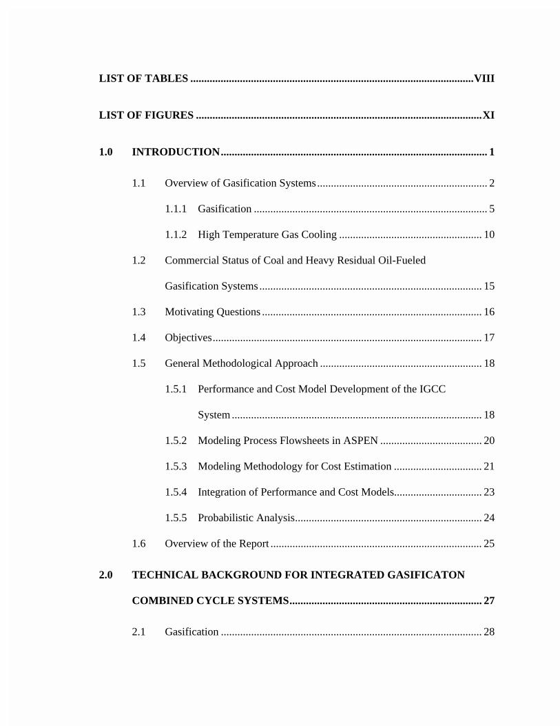
LIST OF TABLES .......................................................................................................VIII
LIST OF FIGURES ........................................................................................................XI
1.0 INTRODUCTION................................................................................................. 1
1.1 Overview of Gasification Systems.............................................................. 2
1.1.1 Gasification ..................................................................................... 5
1.1.2 High Temperature Gas Cooling .................................................... 10
1.2 Commercial Status of Coal and Heavy Residual Oil-Fueled
Gasification Systems ................................................................................. 15
1.3 Motivating Questions ................................................................................ 16
1.4 Objectives.................................................................................................. 17
1.5 General Methodological Approach ........................................................... 18
1.5.1 Performance and Cost Model Development of the IGCC
System ........................................................................................... 18
1.5.2 Modeling Process Flowsheets in ASPEN ..................................... 20
1.5.3 Modeling Methodology for Cost Estimation ................................ 21
1.5.4 Integration of Performance and Cost Models................................ 23
1.5.5 Probabilistic Analysis.................................................................... 24
1.6 Overview of the Report ............................................................................. 25
2.0 TECHNICAL BACKGROUND FOR INTEGRATED GASIFICATON
COMBINED CYCLE SYSTEMS...................................................................... 27
2.1 Gasification ............................................................................................... 28
ii
2.2 High-Temperature Gas Cooling ................................................................ 30
2.3 Gas Scrubbing Process and Low Temperature Gas Cooling .................... 30
2.4. Sulfur Removal Process ............................................................................ 31
2.5 Fuel Gas Saturation and Combustion........................................................ 31
2.6 Combined Cycle........................................................................................ 34
3.0 DOCUMENTATION OF THE PLANT PERFORMANCE
SIMULATION MODEL IN ASPEN OF THE COAL-FUELED
TEXACO-GASIFIER BASED IGCC SYSTEM WITH RADIANT AND
CONVECTIVE HIGH TEMPERATURE GAS COOLING .......................... 36
3.1 Process Description ................................................................................... 36
3.2 Major Process Sections in the Radiant and Convective IGCC Model ...... 40
3.2.1 Coal Slurry and Oxidant Feed to the Gasifier ............................... 40
3.2.2 Gasification ................................................................................... 42
3.2.3 High-Temperature Gas Cooling and Particulate Removal............ 47
3.2.4 Low-Temperature Gas Cooling and Fuel Gas Saturation ............. 51
3.2.5 Gas Turbine ................................................................................... 57
3.2.6 Steam Cycle................................................................................... 72
3.2.7 Plant Energy Balance .................................................................... 84
3.3 Convergence Sequence.............................................................................. 86
3.4 Environmental Emissions.......................................................................... 87
3.4.1 NOx Emissions............................................................................... 88
3.4.2 Particulate Matter Estimations ...................................................... 88
iii
3.4.3 CO and CO2 Emissions ................................................................. 88
3.4.4 SO2 Emissions ............................................................................... 89
4.0 DOCUMENTATION OF THE AUXILIARY POWER MODEL FOR
THE COAL-FUELED TEXACO GASIFIER-BASED IGCC SYSTEM
WITH RADIANT AND CONVECTIVE HIGH TEMPERATURE GAS
COOLING ........................................................................................................... 90
4.1 Coal Handling ........................................................................................... 90
4.2 Gasification ............................................................................................... 93
4.3 Other Process areas ................................................................................... 94
4.3.1 Oxidant feed .................................................................................. 95
4.3.2 Low Temperature Gas Cooling ..................................................... 95
4.3.3 Selexol........................................................................................... 96
4.3.4 Claus Plant .................................................................................... 96
4.3.5 Beavon-Stretford Unit ................................................................... 97
4.3.6 Process Condensate Treatment...................................................... 97
4.3.7 Steam Cycle................................................................................... 97
4.3.8 General Facilities........................................................................... 98
4.4 Net Power Output and Plant Efficiency .................................................... 99
iv
5.0 CAPITAL, ANNUAL, AND LEVELIZED COST MODELS OF THE
COAL-FUELED TEXACO GASIFIER-BASED IGCC SYSTEM WITH
RADIANT AND CONVECTIVE HIGH TEMPERATURE GAS
COOLING ......................................................................................................... 101
5.1 Direct Capital Cost .................................................................................. 101
5.1.1 Oxidant Feed Section .................................................................. 105
5.1.2 Coal Handling Section and Slurry Preparation ........................... 106
5.1.3 Gasification Section .................................................................... 108
5.1.4 Low Temperature Gas Cooling ................................................... 109
5.1.5 Selexol Section............................................................................ 110
5.1.6 Claus Sulfur Recovery Section ................................................... 111
5.1.7 Beavon-Stretford Tail Gas Removal Section .............................. 112
5.1.8 Boiler Feedwater System ............................................................ 112
5.1.9 Process Condensate Treatment.................................................... 113
5.1.10 Gas Turbine Section .................................................................... 114
5.1.11 Heat Recovery Steam Generator ................................................. 114
5.1.12 Steam Turbine ............................................................................. 115
5.1.13 General Facilities......................................................................... 116
5.2 Total Plant Costs ..................................................................................... 116
5.3 Total Capital Requirement ...................................................................... 117
5.4 Annual Costs ........................................................................................... 118
5.5 Levelized Costs ....................................................................................... 118
v
6.0 APPLICATION OF THE PERFORMANCE, EMISSIONS, AND COST
MODEL OF THE COAL-FUELED IGCC SYSTEM WITH RADIANT
AND CONVECTIVE GAS COOLING TO A DETERMINISTIC CASE
STUDY ............................................................................................................... 120
6.1 Input Assumptions .................................................................................. 120
6.2 Model Results.......................................................................................... 121
7.0 DOCUMENTATION OF THE PLANT PERFORMANCE, EMISSIONS,
AND COST SIMULATION MODEL IN ASPEN OF THE COAL-
FUELED TEXACO-GASIFIER BASED IGCC SYSTEM WITH TOTAL
QUENCH HIGH TEMPERATURE GAS COOLING.................................. 127
7.1 Major Process Sections in the Total Quench IGCC Process Simulation
Model ...................................................................................................... 127
7.1.1 Gasification and High Temperature Gas Cooling ....................... 128
7.1.2 Low-Temperature Gas Cooling and Fuel Gas Saturation ........... 132
7.1.3 Steam Cycle................................................................................. 141
7.1.4 Plant Energy Balance .................................................................. 149
7.2 Convergence Sequence............................................................................ 153
7.3 Environmental Emissions........................................................................ 153
7.4 Capital Cost Model ................................................................................. 154
7.4.1 Gasification Section .................................................................... 154
7.4.2 Low Temperature Gas Cooling ................................................... 156
7.4.3 Selexol Section............................................................................ 157
vi
8.0 APPLICATION OF THE PERFORMANCE, EMISSIONS, AND COST
MODEL OF THE COAL-FUELED IGCC SYSTEM WITH TOTAL
QUENCH GAS COOLING TO A DETERMINISTIC CASE STUDY....... 158
8.1 Input Assumptions .................................................................................. 158
8.2 Model Results.......................................................................................... 159
9.0 UNCERTAINTY ANALYSIS.......................................................................... 165
9.1 Methodology for Probabilistic Analysis ................................................. 166
9.1.1 Characterizing Uncertainties ....................................................... 166
9.1.2 Types of Uncertain Quantities..................................................... 168
9.1.3 Some Types of Probability Distributions .................................... 170
9.1.4 Monte Carlo Simulation.............................................................. 172
9.1.5 Methods for Identifying Key Sources of Uncertainty in Model
Inputs........................................................................................... 174
9.2 Input Assumptions for Probabilistic Case Studies .................................. 176
9.3 Probabilistic Analysis of the IGCC Model ............................................. 185
9.4 Model Results and Applications ............................................................. 191
9.5 Analysis of Results.................................................................................. 196
9.5.1 Plant Thermal Efficiency ............................................................ 197
9.5.2 Total Capital Cost ....................................................................... 201
9.5.3 Cost of Electricity........................................................................ 208
9.6 Discussion ............................................................................................... 213
10.0 CONCLUSIONS ............................................................................................... 214
vii
11.0 REFERENCES.................................................................................................. 220
APPENDIX A: GLOSSARY OF ASPEN UNIT OPERATION BLOCKS AND
BLOCK PARAMETERS ................................................................................. 228
APPENDIX B: RESULTS OF THE PERFORMANCE AND COST MODELS
OF THE IGCC SYSTEMS............................................................................... 234
APPENDIX C: PARTIAL RANK CORRELATION COEFFICIENTS FOR
THE IGCC SYSTEMS ..................................................................................... 252
viii
LIST OF TABLES
Table 1.1 IGCC Projects Under Operation or Construction........................................ 16
Table 3.1 Proximate and Ultimate Analysis of the Base Case Illinois No.6Coal.............................................................................................................. 42
Table 3.2 Gasification Section Unit Operation Block Description ............................. 46
Table 3.3 High-Temperature Gas Cooling (Solids Separation) Section UnitOperation Block Description ....................................................................... 51
Table 3.4 Low Temperature Gas Cooling Section Unit Operation BlockDescription................................................................................................... 55
Table 3.5 Gas Turbine Section Unit Operation Block Description ............................. 60
Table 3.6 Steam Cycle Section Unit Operation Block Description............................. 76
Table 3.7 HRSG Section Unit Operation Block Description ...................................... 78
Table 3.8 Auxiliaries Section Unit Operation Block Description ............................... 80
Table 3.9 Steam Turbine Section Unit Operation Block Description ......................... 84
Table 4.1 Summary of Design Studies used for Coal Handling and SlurryPreparation Auxiliary Power Model Development ..................................... 92
Table 5.1 Process Areas for Cost Estimation of an IGCC System. ........................... 102
Table 5.2 Plant Cost Index Values ............................................................................ 104
Table 6.1 Summary of Selected Base Case Input Values for the TexacoGasifier-Based IGCC System with Radiant and Convective HighTemperature Gas Cooling.......................................................................... 124
Table 6.2 Summary of Selected Performance Model of the Coal-Fuel Systemwith Radiant and Convective High Temperature Gas Cooling PointEstimate Results from the Example Case Study ....................................... 125
Table 6.3 Summary of Cost Model Results for the Example Case Study (1998Dollars) ...................................................................................................... 126
ix
Table 7.1 Gasification Section Unit Operation Block Description ........................... 131
Table 7.2 Low Temperature Gas Cooling Section Unit Operation BlockDescription................................................................................................. 134
Table 7.3 HRSG Section Unit Operation Block Description .................................... 144
Table 7.4 Auxiliaries Section Unit Operation Block Description ............................. 146
Table 7.5 Steam Turbine Section Unit Operation Block Description ....................... 149
Table 8.1 Summary of the Base Case Parameters Values for the Texaco CoalGasification Total Quench System ............................................................ 161
Table 8.2 Summary of Selected Performance Model Results from the ExampleCase Study ................................................................................................. 162
Table 8.3 Summary of Cost Model Results for the Example Case Study (1998Dollars) ...................................................................................................... 163
Table 9.1 Summary of the Base Case Parameter Values and Uncertainties forthe Coal-Fueled Texaco Gasifier-Based IGCC System with Radiantand Convective High Temperature Gas Cooling....................................... 179
Table 9.2 Summary of the Base Case Parameter Values and Uncertainties forthe Coal-Fueled Texaco Gasifier-Based IGCC System with TotalQuench High Temperature Gas Cooling ................................................... 182
Table 9.3 List of Uncertainty Variables Used in Each of the Case Studies............... 189
Table 9.4 List of Uncertainty Variables Used in Each of the Case Studies............... 190
Table 9.5 Selected Outputs Collected by the Model for Uncertainty Analysis ......... 194
Table 9.6 Selected Outputs Collected by the Model for Uncertainty Analysis ......... 195
Table 9.7 Summary of Results from Deterministic and ProbabilisticSimulations of IGCC with Original and Screened Sets ofUncertainties .............................................................................................. 199
Table 9.8 Summary of Results from Deterministic and ProbabilisticSimulations of IGCC with Original and Screened Sets ofUncertainties .............................................................................................. 201
Table A.1 ASPEN Unit Operation Block Description ............................................... 228
Table A.2 ASPEN Block Parameters Description...................................................... 232

x
xi
LIST OF FIGURES
Figure 1.1 Conceptual Diagram of an IGCC system ...................................................... 2
Figure 1.2 Radiant and Convective High Temperature Syngas Cooling Design.......... 12
Figure 1.3 Total Quench High Temperature Syngas Cooling Design .......................... 14
Figure 2.1 Temperature Variation in an Entrained Gasifier.......................................... 29
Figure 2.2 Fuel Gas Saturator ....................................................................................... 33
Figure 2.3 Simplified Schematic of Fuel Gas Saturation.............................................. 34
Figure 3.1 IGCC System............................................................................................... 39
Figure 3.2 Gasification Flowsheet ................................................................................ 45
Figure 3.3 Solids Separation Flowsheet........................................................................ 50
Figure 3.4 Low Temperature Gas Cooling Flowsheet .................................................. 54
Figure 3.5 Fuel Gas Saturation Flowsheet .................................................................... 55
Figure 3.6 Gas Turbine Flowsheet ................................................................................ 59
Figure 3.7 Plots of (a) Exhaust Gas Temperature , (b) Simple Cycle Efficiency,and (c) Output versus Gas Turbine Compressor IsentropicEfficiency..................................................................................................... 71
Figure 3.8 Steam Cycle Flowsheet ............................................................................... 75
Figure 3.9 HRSG Section Flowsheet ............................................................................ 77
Figure 3.10 Auxiliaries Flowsheet .................................................................................. 79
Figure 3.11 Steam Turbine Flowsheet ............................................................................ 83
Figure 4.1 Power Requirement for the Coal Slurry Preparation Unit........................... 93
Figure 5.1 Direct Cost for the Coal Handling and Slurry Preparation ProcessArea............................................................................................................ 107
Figure 7.1 Gasification Flowsheet .............................................................................. 130
Figure 7.2 Low Temperature Gas Cooling Flowsheet ................................................ 133
xii
Figure 7.3 Fuel Gas Saturation Flowsheet .................................................................. 140
Figure 7.4 HRSG Section Flowsheet .......................................................................... 143
Figure 7.5 Auxiliaries Flowsheet ................................................................................ 145
Figure 7.6 Steam Turbine Flowsheet .......................................................................... 148
Figure 7.7 Power Requirement for the Gasification Section for Total Quench.......... 151
Figure 7.8 Direct Cost for Total Quench Cooled Gasifier .......................................... 156
Figure 9.1 Examples of Probability Density Functions .............................................. 171
Figure 9.2 Comparison of Probabilistic Results for Cases 2 and 5 for thePlantThermal Efficiency for Radiant and Convective Model............................ 198
Figure 9.3 Comparison of Probabilistic Results for Cases 2 and 5 for thePlantThermal Efficiency for Total Quench Coal Model.................................... 200
Figure 9.4 Comparison of Probabilistic Results for Cases 1 and 4 for theTotalCapital Requirement for Radiant and Convective Model.......................... 203
Figure 9.5 Comparison of Probabilistic Results for Cases 2 and 5 for theTotalCapital Requirement for Radiant and Convective Model.......................... 204
Figure 9.6 Comparison of Probabilistic Results for Cases 3 and 6 for theTotalCapital Requirement for Radiant and Convective Model.......................... 204
Figure 9.7 Comparison of Probabilistic Results for Cases 1 and 4 for theTotalCapital Requirement for Total Quench Coal Model.................................. 206
Figure 9.8 Comparison of Probabilistic Results for Cases 2 and 5 for theTotalCapital Requirement for Total Quench Coal Model.................................. 207
Figure 9.9 Comparison of Probabilistic Results for Cases 3 and 6 for theTotalCapital Requirement for Total Quench Coal Model.................................. 207
Figure 9.10 Comparison of Probabilistic Results for Cases 1 and 4 for theLevelized Cost of Electricity for Radiant and Convective Model............. 209
Figure 9.11 Comparison of Probabilistic Results for Cases 2 and 5 for theLevelized Cost of Electricity for Radiant and Convective Model............. 210
Figure 9.12 Comparison of Probabilistic Results for Cases 3 and 6 for theLevelized Cost of Electricity for Radiant and Convective Model............. 210
xiii
Figure 9.13 Comparison of Probabilistic Results for Cases 1 and 4 for theLevelized Cost of Electricity for Total Quench Coal Model..................... 211
Figure 9.14 Comparison of Probabilistic Results for Cases 2 and 5 for theLevelized Cost of Electricity for Total Quench Coal Model..................... 212
Figure 9.15 Comparison of Probabilistic Results for Cases 3 and 6 for theLevelized Cost of Electricity for Total Quench Coal Model..................... 212
1
1.0 INTRODUCTION
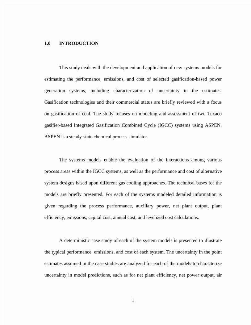
This study deals with the development and application of new systems models for
estimating the performance, emissions, and cost of selected gasification-based power
generation systems, including characterization of uncertainty in the estimates.
Gasification technologies and their commercial status are briefly reviewed with a focus
on gasification of coal. The study focuses on modeling and assessment of two Texaco
gasifier-based Integrated Gasification Combined Cycle (IGCC) systems using ASPEN.
ASPEN is a steady-state chemical process simulator.
The systems models enable the evaluation of the interactions among various
process areas within the IGCC systems, as well as the performance and cost of alternative
system designs based upon different gas cooling approaches. The technical bases for the
models are briefly presented. For each of the systems modeled detailed information is
given regarding the process performance, auxiliary power, net plant output, plant
efficiency, emissions, capital cost, annual cost, and levelized cost calculations.
A deterministic case study of each of the system models is presented to illustrate
the typical performance, emissions, and cost of each system. The uncertainty in the point
estimates assumed in the case studies are analyzed for each of the models to characterize
uncertainty in model predictions, such as for net plant efficiency, net power output, air
2
pollutant emissions, and capital, annual, and levelized costs. The key uncertainties with
respect to plant efficiency and cost are identified. The Texaco gasifier-based IGCC
models are intended for use as benchmarks in comparisons with other coal/fuel-based
power generation systems, models for many of which have been developed in previous
work (Frey and Rubin, 1990; Frey and Rubin, 1991; Frey and Rubin, 1992a; Frey and
Rubin, 1992b; Frey, 1994; Frey and Williams, 1995; Frey et al, 1994; Agarwal and Frey,
1995; Agrawal and Frey, 1997; Bharvirkar and Frey, 1998). Thus, the models presented
here are several of a set of complimentary models that enable comparisons of competing
systems for strategic planning purposes.
1.1 Overview of Gasification Systems
Gasification systems are a promising approach for clean and efficient power
generation as well as for polygeneration of a variety of products, such as steam, sulfur,
hydrogen, methanol, ammonia, and others (Philcox and Fenner, 1996). As of 1996, there
were 354 gasifiers located at 113 facilities worldwide. The gasifiers use natural gas,
petroleum residuals, petroleum coke, refinery wastes, coal, and other fuels as inputs, and
produce a synthesis gas containing carbon monoxide (CO), hydrogen (H2), and other
components. The syngas can be processed to produce liquid and gaseous fuels, chemicals,
and electric power. In recent years, gasification has received increasing attention as an
option for repowering at oil refineries, where there is currently a lack of markets for low-
value liquid residues and coke (Simbeck, 1996).
3
A general category of gasification-based systems is Integrated Gasification
Combined Cycle (IGCC) systems. IGCC is an advanced power generation concept with
the flexibility to use coal, heavy oils, petroleum coke, biomass, and waste fuels to
produce electric power as a primary product. IGCC systems typically produce sulfur as a
byproduct. Systems that produce many co-products are referred to as "polygeneration"
systems. IGCC systems are characterized by high thermal efficiencies and lower
environmental emissions than conventional pulverized coal fired plants (Bjorge, 1996).
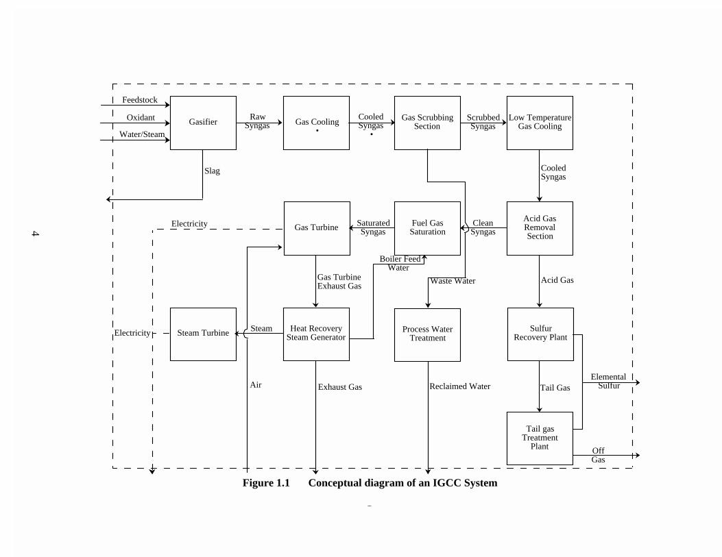
A generic IGCC system is illustrated schematically in Figure 1.1. In an IGCC
power plant, the feedstock to the gasifier is converted to a syngas, composed mainly of
hydrogen and carbon monoxide, using a gasification process. After passing through a gas
cleanup system, in which particles and soluble gases are removed via wet scrubbing and
in which sulfur is removed and recovered via a selective removal process, the syngas is
utilized in a combined cycle power plant. Different variations of IGCC systems exist
based upon the type of coal gasifier technology, oxidant (e.g., oxygen or air), and gas
cleanup system employed.
1
4
Gasifier Gas Cooling •
Low Temperature Gas Cooling
Gas Scrubbing Section
Acid Gas Removal Section
Gas Turbine
Heat Recovery Steam GeneratorSteam Turbine
Feedstock
Oxidant Raw Syngas
Cooled Syngas
•
Scrubbed Syngas
Cooled Syngas
Clean Syngas
Gas Turbine Exhaust Gas
Exhaust Gas
Steam
Slag
Sulfur Recovery Plant
Tail gas Treatment
Plant
Acid Gas
Off Gas
Elemental SulfurTail Gas
Electricity
Air
Fuel Gas Saturation
Saturated Syngas
Waste Water
Water/Steam
Electricity
Process Water Treatment
Reclaimed Water
Boiler Feed Water
Figure 1.1 Conceptual diagram of an IGCC System
5
A typical IGCC system includes process sections of Fuel Handling, Gasification,
High-Temperature Gas Cooling, Low Temperature Gas Cooling and Gas Scrubbing, Acid
Gas Separation, Fuel Gas Saturation, Gas Turbine, Heat Recovery Steam Generator,
Steam Turbine, and Sulfur Byproduct Recovery. The specific design of each of the
process sections such as gasification and high-temperature gas cooling varies in different
IGCC systems.
1.1.1 Gasification
Three generic designs of gasification are typically employed in IGCC systems,
each of which are described below. In all types of reactors, the feedstock fuel is converted
to syngas in reactors with an oxidant and either steam or water. The oxidant is required to
partially oxidize the fuel. The exothermic oxidation process provides heat for the
endothermic gasification reactions. Water or steam is used as a source of hydrolysis in the
gasification reactions. The type of reactor used is the primary basis for classifying
different types of gasifiers.
1.1.1.1 Moving-Bed or Counter-Current Reactors
Moving bed reactors feature counter-current flow of fuel with respect to both the
oxidant and the steam. For example, in the case of coal gasification, coal particles of
approximately 4 mm to 30 mm (Simbeck et al., 1983) in diameter are introduced at the
top of the reactor, and move downward. Oxidant is introduced at the bottom of the
reactor. A combustion zone at the bottom of the reactor produces thermal energy required
6
for gasification reactions, which occur primarily in the central zone of the reactor. Steam
is also introduced near the bottom of the gasifier. As the hot gases from combustion and
gasification move upward, they come into contact with the fuel introduced at the top. The
heating of the fuel at the top of the reactor results in devolatilization, in which lighter
hydrocarbon compounds are driven off and exit as part of the syngas. Because the gases
leaving the gasifier contact the relatively cool fuel entering the gasifier, the exit syngas
temperature is relatively low compared to other types of reactors. The counter-current
flow of fuel with the oxidant and steam can result in efficient utilization of the fuel, as
long as the residence time of the fuel is long enough for even the larger particles to be
fully consumed. Ash and unconverted fuel exit the bottom of the gasifier via a rotating
grate.
A typical syngas exit temperature for a moving bed gasifier is approximately
1,100 oF. At this temperature, some of the heavier volatilized hydrocarbon compounds,
such as tars and oils, will not be cracked and can easily condense in downstream syngas
cooling equipment. Because fuel is introduced at the top of the gasifier where the syngas
is exiting, this type of gasifier cannot handle fine fuel particles. Such particles would be
entrained with the exiting syngas and would not be converted to syngas in the reactor bed.
Cyclones are typically used to capture fine particles in the syngas, which are often sent to
a briquetting facility to form larger particles and then recycled to the gasifier for another
attempt at conversion.
7
An overall measure of gasifier performance is the cold gas efficiency. The cold
gas efficiency is the ratio of the heating value of "cold" syngas, at standard temperature,
to the heating value of the amount of fuel consumed required to produce the syngas. The
cold gas efficiency does not take into account recovery of energy in the gasifier such as
through steam generation or associated with sensible heat of the syngas at high
temperatures. Moving bed gasifiers tend to have very high cold gas efficiencies, with
values in the range of 80 to 90 percent.
Typical examples of such reactors are Lurgi dry bottom gasifiers and the British
Gas/Lurgi slagging gasifiers.
1.1.1.2 Fluidized-Bed Gasifiers
Fluidized bed reactors feature rapid mixing of fuel particles in a 0.1 mm to 10 mm
size range with both oxidant and steam in a fluidized bed. The feedstock fuel, oxidant and
steam are introduced at the bottom of the reactor. In these reactors, backmixing of
incoming feedstock fuel, oxidant, steam, and the fuel gas takes place resulting in a
uniform distribution of solids and gases in the reactors. The gasification takes place in the
central zone of the reactor. The coal bed is fluidized as the fuel gas flow rate increases
and becomes turbulent when the minimum fluidizing velocity is exceeded.
The reactors have a narrow temperature range of 1800 oF to 1900 oF. The fluidized
bed is maintained at a nearly constant temperature, which is well below the initial ash
8
fusion temperature to avoid clinker formation and possible defluidization of the bed.
Unconverted coal in the form of char is entrained from the bed and leaves the gasifier
with the hot raw gas. This char is separated from the raw gas in the cyclones and is
recycled to the hot ash agglomerating zone at the bottom of the gasifier. The temperature
in that zone is high enough to gasify the char and reach the softening temperature for
some of the eutectics in the ash. The ash particles stick together, grow in size and become
dense until they are separated from the char particles, and then fall to the base of the
gasifier, where they are removed.
The processes in these reactors are restricted to reactive, non-caking coals to
facilitate easy gasification of the unconverted char entering the hot ash zone and for
uniform backmixing of coal and fuel gas. The cold gas efficiency is approximately 80
percent (Supp, 1990). These reactors have been used for Winkler gasification process and
High-temperature Winkler gasification process. A key example of fluidized gasification
design is the KRW gasifier.
1.1.1.3 Entrained-Flow Reactors
The entrained-flow process features a plug type reactor where the fine feedstock
fuel particles (less than 0.1 mm) flow co-currently and react with oxidant and/or steam.
The feedstock, oxidant and steam are introduced at the top of the reactor. The gasification
takes place rapidly at temperatures in excess of 2300 oF. The feedstock is converted
primarily to H2, CO, and CO2 with no liquid hydrocarbons being found in the syngas. The
9
raw gas leaves from the bottom of the reactor at high temperatures of 2300 oF and greater.
The raw gas has low amounts of methane and no other hydrocarbons due to the high
syngas exit temperatures.
The entrained flow gasifiers typically use oxygen as the oxidant and operate at
high temperatures well above ash slagging conditions in order to assure reasonable
carbon conversion and to provide a mechanism for slag removal (Simbeck et al., 1983).
Entrained-flow gasification has the advantage over the other gasification designs in that it
can gasify almost all types of coals regardless of coal rank, caking characteristics, or the
amount of coal fines. This is because of the relatively high temperatures which enable
gasification of even relatively unreactive feedstocks that might be unsuitable for the
lower temperature moving bed or fluidized bed reactors. However, because of the high
temperatures, entrained-flow gasifiers use more oxidant than the other designs. The cold
gas efficiency is approximately 80 percent (Supp, 1990). Typical examples of such
reactors are Texaco Gasifiers and Destec Gasifiers.
The advantage of adopting entrained flow gasification over the above mentioned
reactors is the high yield of synthesis gas containing insignificant amounts of methanol
and other hydrocarbons as a result of the high temperatures in the entrained-flow reactors.
Texaco gasification is a specialized form of entrained flow gasification in which
coal is fed to the gasifier in a water slurry. Because of the water in the slurry, which acts
10
as heat moderator, the gasifier can be operated at higher pressures than other types of
entrained-flow gasifiers. Higher operating pressure leads to increased gas production
capability per gasifier of a given size (Simbeck et al., 1983)
In this study, we focus on modeling assessment of entrained flow gasification.
Assessments of moving bed and fluidized bed gasifier based systems have been done in
previous work (Frey and Rubin, 1992a, 1992b, Frey et al., 1994, Frey, 1998).
1.1.2 High Temperature Gas Cooling
The design of the high temperature syngas cooling process area depends on the
type of gasifier used. The gas cooling requirements for entrained flow gasification
systems are more demanding than for other gasification systems as the former produce
syngas at higher temperatures. Typically, the gas cooling process for systems employing
entrained flow gasification systems either use heat exchangers to recover thermal energy
and generate steam or use water quenching. The former design can be radiant and
convective or radiant only, while the latter is known as total quench high temperature gas
cooling. The former is more efficient as it can produce high temperature and pressure
steam, whereas the latter is much less expensive (Doering and Mahagaokar, 1992).
11
1.1.2.1 Radiant and Convective Syngas Cooling Design
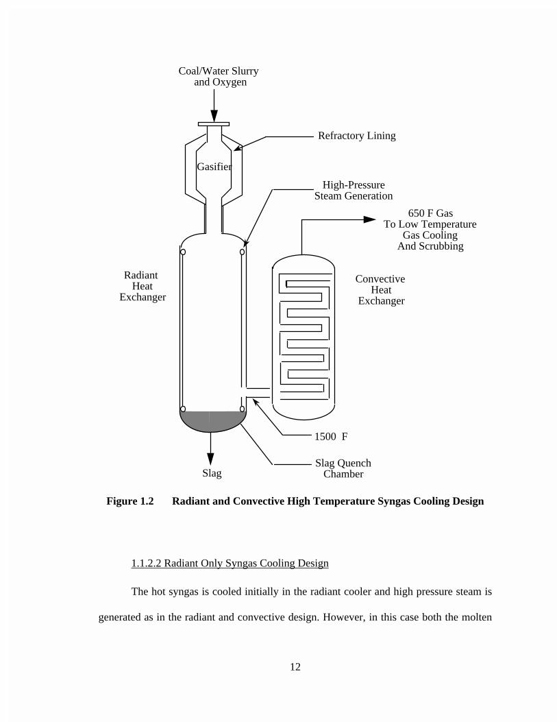
The design of a radiant and convective gasification system is shown in Figure 1.2.
Each gasifier has one radiant cooler and one convective cooler. The hot syngas is initially
cooled in an radiant heat transfer type of heat exchanger. High pressure steam is
generated in tubes built into the heat transfer surface at the perimeter of the cylindrical
gas flow zone. The molten slag drops into a slag quench chamber at the bottom of the
radiant gas cooler where it is cooled and removed for disposal. The gas leaves the radiant
cooler at a temperature of approximately 1500 oF.
The syngas from the radiant heat exchanger flows into a convection type of heat
exchanger. In the convective heat exchanger, the syngas flows across the boiler tube
banks. These tubes help remove the entrained particles in the syngas that are too fine to
drop out in the bottom of the radiant cooler. High pressure steam is generated in these
tubes. The cooled gas leaves the convective chamber at a temperature of approximately
650 oF.
12
Coal/Water Slurry and Oxygen
Slag
Refractory Lining
High-Pressure Steam Generation
Slag Quench Chamber
1500 F
Convective Heat
Exchanger
650 F Gas To Low Temperature
Gas Cooling And Scrubbing
Gasifier
Radiant Heat
Exchanger
Figure 1.2 Radiant and Convective High Temperature Syngas Cooling Design
1.1.2.2 Radiant Only Syngas Cooling Design
The hot syngas is cooled initially in the radiant cooler and high pressure steam is
generated as in the radiant and convective design. However, in this case both the molten
13
slag and the raw gas are quenched in the water pool at the bottom of the radiant cooler.
The cooled slag is removed from the cooler for disposal. The raw gas, saturated with
moisture, flows out of the radiant cooler at a temperature of approximately 400 oF.
1.1.2.3 Total Quench Design
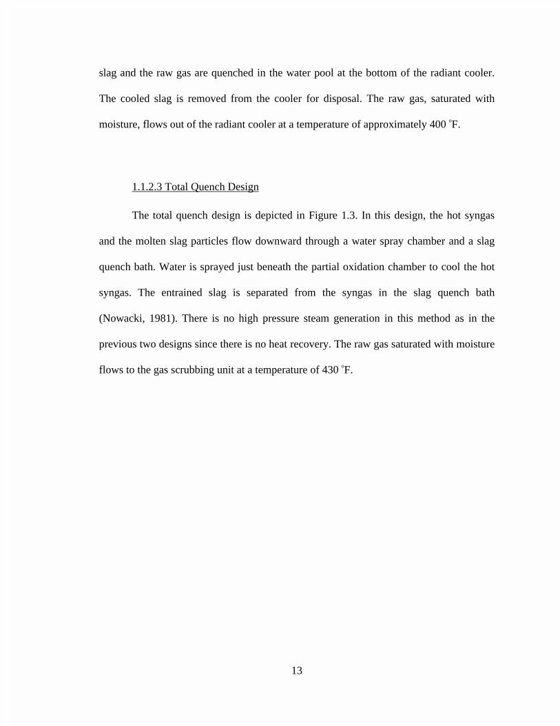
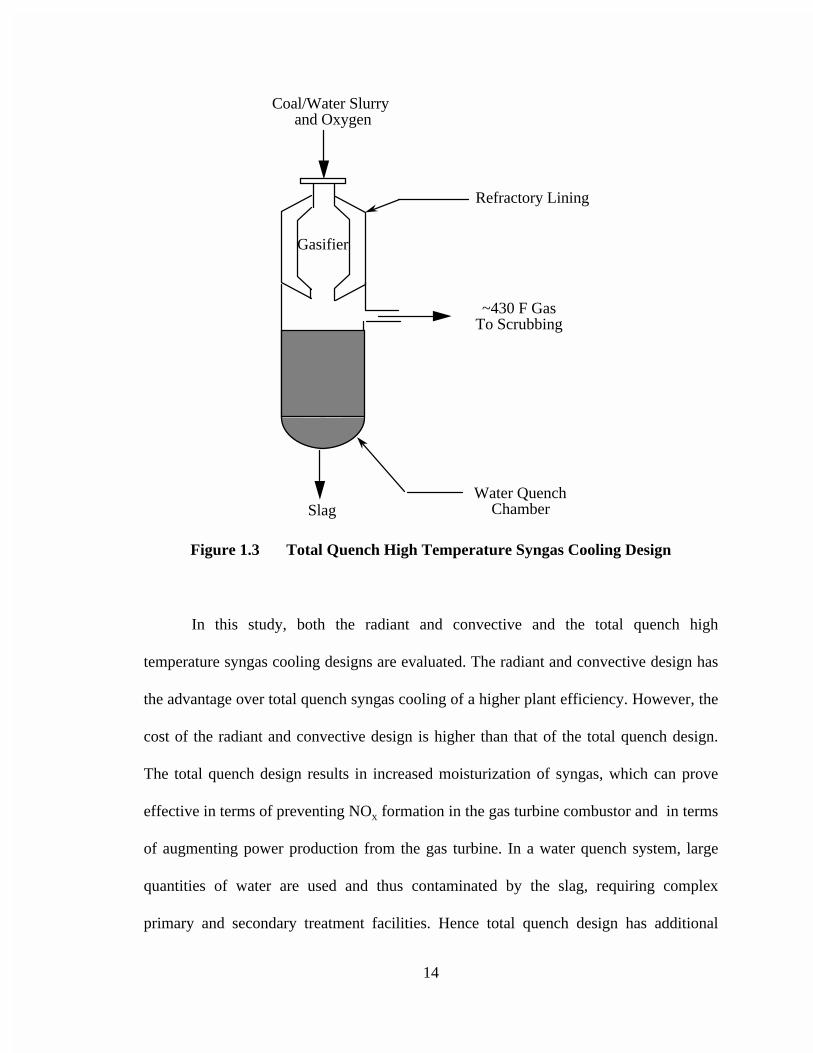
The total quench design is depicted in Figure 1.3. In this design, the hot syngas
and the molten slag particles flow downward through a water spray chamber and a slag
quench bath. Water is sprayed just beneath the partial oxidation chamber to cool the hot
syngas. The entrained slag is separated from the syngas in the slag quench bath
(Nowacki, 1981). There is no high pressure steam generation in this method as in the
previous two designs since there is no heat recovery. The raw gas saturated with moisture
flows to the gas scrubbing unit at a temperature of 430 oF.
14
Coal/Water Slurry and Oxygen
Refractory Lining
SlagWater Quench
Chamber
~430 F Gas To Scrubbing
Gasifier
Figure 1.3 Total Quench High Temperature Syngas Cooling Design
In this study, both the radiant and convective and the total quench high
temperature syngas cooling designs are evaluated. The radiant and convective design has
the advantage over total quench syngas cooling of a higher plant efficiency. However, the
cost of the radiant and convective design is higher than that of the total quench design.
The total quench design results in increased moisturization of syngas, which can prove
effective in terms of preventing NOX formation in the gas turbine combustor and in terms
of augmenting power production from the gas turbine. In a water quench system, large
quantities of water are used and thus contaminated by the slag, requiring complex
primary and secondary treatment facilities. Hence total quench design has additional
15
operating problems such as those caused due to increased water treating facilities,
increased discharge water permitting issues, and added operating and maintenance costs
when compared to radiant and convective design (Doering and Mahagaokar, 1992).
1.2 Commercial Status of Coal and Heavy Residual Oil-Fueled GasificationSystems
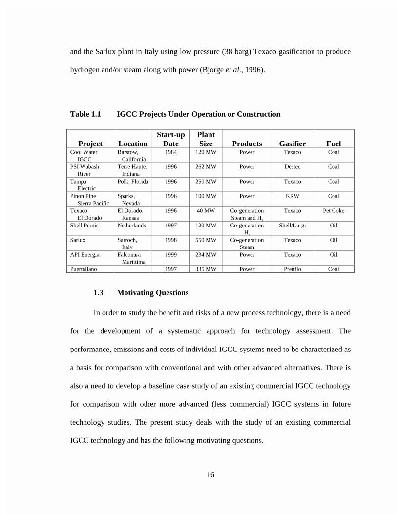
The IGCC concept has been demonstrated commercially. Table 1.1 lists the IGCC
plants currently in operation or undergoing construction. The Texaco coal gasification
process has been successfully used in a number of chemical plants since the early 1980s
for the production of synthesis gas from coal. A Texaco-based 95 MW IGCC power plant
was operated successfully from 1984 to 1988 in California (Simbeck et al., 1996). API
Energia, a joint venture of Asea Brown Boveri and API, adopted Texaco gasification to
gasify visbreaker residue from an API refinery to produce steam and power. Tampa
Electric Company’s Polk Power station also utilizes Texaco gasification, gasifying about
2,000 tons of coal per day to produce 250 MW of power. The El Dorado gasification
project demonstrates that hazardous waste streams can be converted by gasification to
valuable products. (Farina et al., 1998).
A Destec gasifier-based IGCC power plant at Wabash River Station is currently
under operation (Simbeck et al., 1996). A 335 MW IGCC demonstration plant for
European electricity companies is operating at Puertollano, Spain (Mendez-vigo et al.,
1998). The Texaco gasifier-based El Dorado plant, the Shell-Pernis plant in Netherlands,
16
and the Sarlux plant in Italy using low pressure (38 barg) Texaco gasification to produce
hydrogen and/or steam along with power (Bjorge et al., 1996).
Table 1.1 IGCC Projects Under Operation or Construction
Project LocationStart-up
DatePlantSize Products Gasifier Fuel
Cool Water IGCC
Barstow, California
1984 120 MW Power Texaco Coal
PSI Wabash River
Terre Haute, Indiana
1996 262 MW Power Destec Coal
Tampa Electric
Polk, Florida 1996 250 MW Power Texaco Coal
Pinon Pine Sierra Pacific
Sparks, Nevada
1996 100 MW Power KRW Coal
Texaco El Dorado
El Dorado, Kansas
1996 40 MW Co-generationSteam and H2
Texaco Pet Coke
Shell Pernis Netherlands 1997 120 MW Co-generationH2
Shell/Lurgi Oil
Sarlux Sarroch, Italy
1998 550 MW Co-generationSteam
Texaco Oil
API Energia Falconara Marittima
1999 234 MW Power Texaco Oil
Puertallano 1997 335 MW Power Prenflo Coal
1.3 Motivating Questions
In order to study the benefit and risks of a new process technology, there is a need
for the development of a systematic approach for technology assessment. The
performance, emissions and costs of individual IGCC systems need to be characterized as
a basis for comparison with conventional and with other advanced alternatives. There is
also a need to develop a baseline case study of an existing commercial IGCC technology
for comparison with other more advanced (less commercial) IGCC systems in future
technology studies. The present study deals with the study of an existing commercial
IGCC technology and has the following motivating questions.
17
1. What are the thermal efficiencies, emissions, and costs of selected entrained-flow
gasification-based IGCC systems when fueled by coal?
2. How does the design of the high temperature gas cooling system of a coal-fueled
IGCC system affect the performance, emissions, and costs?
3. What are the uncertainties in the point estimates assumed for the IGCC systems?
4. What are the key sources of uncertainty in the performance, emissions, and costs
of the technologies?
1.4 Objectives
The objectives of the current work are:
1. To develop new systems models based upon the best available information
regarding process performance, emissions and cost for the following
configurations:
(a) Oxygen-blown coal-fueled Texaco gasifier-based IGCC system with
radiant and convective high temperature syngas cooling; and
(b) Oxygen-blown coal-fueled Texaco gasifier-based IGCC system with total
quench high temperature syngas cooling.
2. To verify the models;
3. To compare the high temperature syngas cooling designs;
18
4. To characterize uncertainty in the performance, emissions, and costs of these
systems to provide insight into the potential pay-offs and downside risks of these
technologies.
1.5 General Methodological Approach
This section describes the methodologies adopted for the development of
performance, emissions and costs of two IGCC systems and the integration of the
performance and cost models. The requirement for a probabilistic analysis of the models
developed is also discussed.
1.5.1 Performance and Cost Model Development of the IGCC System
The Federal Energy Technology Center (FETC) of the U.S. Department of Energy
has developed a number of performance simulations of IGCC systems in the ASPEN
modeling environment. A number of these models have been refined by Frey and others
(Frey and Rubin, 1991, Frey et al., 1994, Frey, 1998) in order to calculate mass and
energy balances for IGCC systems, conduct sensitivity analyses of performance
parameters, track environmental species, and evaluate design modifications. Subroutines
that calculate capital, annual, and levelized costs have also been developed and
incorporated with the refined performance models.
19
The Texaco gasifier-based IGCC system models developed in this study are based
primarily on the general configuration and design basis of a study sponsored by the
Electric Power Research Institute (EPRI) (Matchak et al., 1984). K.R. Stone developed a
process simulation model based on the radiant and convective high temperature gas
cooling design in 1985 at FETC. This FETC model has been substantially refined for this
study.
The IGCC simulation models of radiant and convective gasifier design and total
quench high temperature gas cooling design developed in the present study are intended
to predict the output values of process performance measures (e.g., plant thermal
efficiency) for a given set of input assumptions. The key refinements to the earlier FETC
model, which are also incorporated into the new model of the total quench based system,
include complete replacement of the gas turbine flowsheet with a more detailed model,
implementation of a more detailed fuel gas saturation model, incorporation of NOx
emissions as a model output, refinement and more comprehensive inclusion of auxiliary
power demand estimates, and implementation of a capital, annual, and levelized cost
model. The key improvements to the original FETC model of the radiant and convective
based system are described in more detail for the gas turbine and the cost model in
Chapters 3.0 and 5.0 and the auxiliary power consumption models are elaborated upon in
Chapter 4.0.
20
1.5.2 Modeling Process Flowsheets in ASPEN
The performance model of the Texaco-based IGCC was developed as an ASPEN
input file. ASPEN is a FORTRAN-based deterministic steady-state chemical process
simulator developed by the Massachusetts Institute of Technology (MIT) for DOE to
evaluate synthetic fuel technologies (MIT, 1987). The ASPEN framework includes a
number of generalized unit operation “blocks”, which are models of specific process
operations or equipment (e.g., chemical reactions, pumps). By specifying configurations
of unit operations and the flow of material, heat, and work streams, it is possible to
represent a process plant in ASPEN. In addition to a varied set of unit operations blocks,
ASPEN also contains an extensive physical property database and convergence
algorithms for calculating results in closed loop systems, all of which make ASPEN a
powerful tool for process simulation.
ASPEN uses a sequential-modular approach to flowsheet convergence. In this
approach, mass and energy balances for individual unit operation blocks are computed
sequentially, often in the same order as the sequencing of mass flows through the system
being modeled. However, when there are recycle loops in an ASPEN flowsheet, stream
and block variables have to be manipulated iteratively in order to converge upon the mass
and energy balance. ASPEN has a capability for converging recycle loops using a feature
known as “tear streams.”
21
In addition to calculations involving unit operations, there are other types of
blocks used in ASPEN to allow for iterative calculations or incorporation of user-created
code. These include design specifications and FORTRAN blocks.
A design specification is used for feedback control. The user can set any
flowsheet variable or function of flowsheet variables to a particular design value. A feed
stream variable or block input variable is designated to be manipulated in order to achieve
the design value. FORTRAN statements can be used within the design specification block
to compute design specification function values.
FORTRAN blocks are used for feedforward control. Any FORTRAN operation
can be carried out on flowsheet variables by using in-line FORTRAN statements that
operate on these variables. FORTRAN blocks are one method for incorporating user code
into the model. It is also possible to call any user-provided subroutine from either a
design specification or FORTRAN block.
1.5.3 Modeling Methodology for Cost Estimation
The variety of approaches available to developing cost estimates for process
plants differ in the level of detail with which costs are separated, as well as in the
simplicity or complexity of analytic relationships used to estimate line item costs. The
level of detail appropriate for the cost estimate depends on: (1) the state of technology
development for the process of interest; and (2) the intended use of the cost estimates.
22
The models developed here are intended to estimate the costs of innovative coal-to-
electricity systems for the purpose of evaluating the comparative economics of alternative
process configurations. The models are intended to be used only for preliminary or “study
grade” estimates using representative (generic) plant designs and parameters.
In the electric utility and chemical process industries, there are generally accepted
guidelines regarding the approach to developing cost estimates. The Electric Power
Research Institute has defined four types of cost estimates: simplified, preliminary,
detailed, and finalized. The cost estimates developed in this work are “preliminary”
(EPRI, 1986). Preliminary cost estimates are appropriate for the purposes of evaluating
alternative technologies, and for research planning. These cost estimates are sensitive to
the performance and design parameters that are most influential in affecting costs (Frey
and Rubin, 1990).
One of the major constraints on the development of the cost model is the
availability of data from which to develop cost versus performance relationships for
specific process area or for major equipment items. Data from published studies can be
used to develop cost models for specific process areas using regression analysis (Frey and
Rubin, 1990).
The new cost models developed for each of the three technologies evaluated in
this work include capital, annual, and levelized costs. The models estimate the direct
23
capital costs of each major plant section as a function of key performance and design
parameters. The total capital cost is calculated based on direct and indirect capital costs.
The total direct cost is a summation of the plant section direct costs and general facilities
cost. The total indirect cost is the sum of indirect construction costs, engineering and
home office fees, sales tax, and environmental permitting costs. The latest process
contingency factors have been incorporated in the cost model and are included in the total
capital cost.
The annual cost model includes both fixed and variable operating costs. Fixed
operating costs include operating labor, maintenance labor and materials, and overhead
costs associated with administrative and support labor. The latest maintenance cost
factors have been included in the cost model in order to calculate process area annual
maintenance cost. Variable operating costs include fuel, consumables, ash disposal, and
byproduct credits. The operating costs are estimated based on 31 cost parameters such as
unit prices and costs (Frey and Rubin, 1990).
1.5.4 Integration of Performance and Cost Models
The cost model has been developed as a FORTRAN subroutine, which is linked
to the ASPEN simulation model. The cost model obtains approximately 50 to 60 process
variables from the ASPEN performance model for use in both the capital and annual cost
calculations. Newly developed regression models are used to calculate the auxiliary
power requirements for many of the process areas. The overall plant efficiency is
24
calculated in the cost model subroutine taking into account the gross gas turbine and
steam turbine output and the auxiliary power demands.
1.5.5 Probabilistic Analysis
The complexity of gasification systems implies that it is difficult to evaluate all
possible combinations of gasification components based upon the relatively small
population of demonstration and commercial plants. For each of the major components
of a typical gasification system (e.g., fuel feed, gasification, syngas cooling, syngas
cleanup, power generation, byproduct recovery), there are many possible options.
Limited performance and cost data for first generation systems, coupled with
uncertainties associated with a large number of alternative process configurations,
motivates a systematic approach to evaluating the risks and potential pay-offs of
alternative concepts.
Technology assessment models are typically developed for the purpose of
providing a point-estimate which may be intended to serve as an accurate and precise
prediction of some quantity (e.g., thermal efficiency, total capital cost). The purpose of
such analyses are to provide decision makers with a best-estimate that can be used in
comparison with other assessments or to develop design targets or budgetary cost
estimates. However, quantitative measures of the accuracy and precision of model
predictions are usually not developed, because no information on model or input
uncertainty is accounted for quantitatively. Deterministic estimates for the performance
25
and cost of new process technologies are often significantly biased toward optimistic
outcomes (Merrow et al., 1981). Such biases can lead to serious misallocation of
resources if decisions are made to pursue research and development on a technology
whose risks were not properly quantified.
To explicitly represent uncertainties in gasification systems and other process
technologies, a probabilistic modeling approach has been developed and applied. This
approach features: (1) development of sufficiently detailed engineering models of
performance, emissions, and cost; (2) implementation of the models in a probabilistic
modeling environment; (3) development of quantitative representations of uncertainties in
specific model parameters based on literature review, data analysis, and elicitation of
technical judgments from experts; (4) identification of key uncertainties in the model
input variables; and (5) modeling applications for cost estimating, risk assessment, and
research planning. The methods have been applied to previous case studies of
gasification and other advanced power generation and environmental control systems
(e.g., Frey and Rubin 1992; Frey et al., 1994).
1.6 Overview of the Report
The organization of the report is as per the following order. Chapter 2 provides a
technical background for Texaco gasifier-based IGCC systems. Chapter 3 elaborates on
26
the development of the performance model of a coal-fueled IGCC system with Texaco
gasifier with radiant and convective design. Chapter 4 documents the auxiliary power
consumption models of the IGCC plant developed in Chapter 3. The direct capital costs
of the IGCC system with the radiant and convective high temperature gas cooling design
are modeled in Chapter 5. The model developed in Chapters 3 to 5 is applied to a
deterministic case study in Chapter 6. Chapters 7 discusses the development of the
performance, emissions, and costs of a coal-fueled Texaco gasifier-based IGCC system
with total quench high temperature gas cooling. Chapter 8 provides the results of
applying the model developed in Chapter 7 to a deterministic case study. Chapter 9
discusses the uncertainty analysis performed on the three IGCC models developed in the
present study. Chapter 10 presents the conclusions obtained from the current study.
27
2.0 TECHNICAL BACKGROUND FOR INTEGRATED GASIFICATONCOMBINED CYCLE SYSTEMS
This study describes performance and cost models for two Texaco gasifier-based
IGCC systems: (1) radiant and convective high temperature syngas cooling using coal;
and (2) total quench high temperature syngas cooling using coal. IGCC systems for
radiant and convective model and total quench model are illustrated schematically in
Figure 1.1. The fuel is fed to the gasifier in a slurry in the case of coal being used as
feedstock. Oxygen is used to combust only a portion of the feedstock in order to provide
thermal energy needed by endothermic gasification reactions. The raw syngas leaves the
gasifier at approximately 2400 oF and cooled either by a series of radiant and convective
heat exchangers to a temperature of 650 oF or by contact with water to a temperature of
433 oF. The syngas passes through a wet scrubbing system to remove particulate matter
and water soluble gases such as NH3.
The scrubbed gas is further cooled to 101 oF prior to entering a Selexol acid gas
separation unit. H2S and COS are removed from the syngas in the Selexol unit and sent to
a Claus plant and a Beavon-Stretford tail gas treatment unit for sulfur recovery. The clean
gas is reheated and saturated with moisture prior to firing in a gas turbine. The saturation
helps prevent formation of thermal NOx during combustion. The hot gas turbine exhaust
passes through a Heat Recovery Steam Generator (HRSG) to provide energy input to a
steam turbine bottoming cycle. Both the gas turbine and the steam turbine generate
power.
28
The details of the major process areas are briefly described.
2.1 Gasification
Texaco gasification can handle a wide variety of feedstocks including coal, heavy
oils, and petroleum coke (Preston, 1996). The current study focuses on IGCC systems
using coal feed. The feed coal is crushed and slurried in wet rod mills. The coal slurry
containing about 66.5 weight percent solids is fed into the gasifier, which is a open,
refractory-lined chamber, together with a feed stream of oxidant. The slurry is transferred
to the gasifier at high pressure through charge pumps. The water in the coal slurry acts as
a temperature moderator and also as a source of hydrogen in gasification (Simbeck et al.,
1983). Oxygen is assumed as the oxidant for the IGCC systems evaluated in this study.
The oxidant stream contains 95 percent pure oxygen. The oxygen is compressed to a
pressure sufficient for introduction into the burner of the Texaco gasifier (Matchak et al.,
1984).
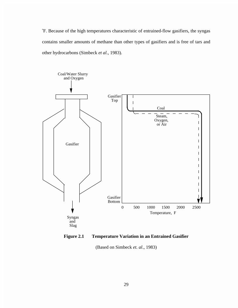
Gasification takes place rapidly at temperatures exceeding 2300 oF. Coal is
partially oxidized at high temperature and pressure. Figure 2.1 demonstrates the
temperature variation across the gasifier (Simbeck et al., 1983). The combustion zone is
near the top of the reactor, where the temperature in the gasifier changes from
approximately 250 to 2500 oF. As a result, a raw gas composed mainly of carbon dioxide,
carbon monoxide, hydrogen, and water vapor is produced. The syngas contains soot
particles. The syngas leaves the gasifier at temperatures in the range of 2300 oF to 2700
29
oF. Because of the high temperatures characteristic of entrained-flow gasifiers, the syngas
contains smaller amounts of methane than other types of gasifiers and is free of tars and
other hydrocarbons (Simbeck et al., 1983).
Gasifier
Coal/Water Slurry and Oxygen
Syngas and Slag
Gasifier Top
Gasifier Bottom
0 500 1000 1500 2000 2500
Steam, Oxygen,
or Air
Temperature, F
Coal
Figure 2.1 Temperature Variation in an Entrained Gasifier
(Based on Simbeck et. al., 1983)
30
2.2 High-Temperature Gas Cooling
In the case of radiant and convective (RC) based system model, the hot gas from
the gasifier is initially cooled in a radiant heat exchanger. High pressure steam is
generated in tubes built into the heat transfer surface at the perimeter of the cylindrical
gas flow zone. Molten slag entrained in the raw gas drops into a water quench pool at the
bottom of the radiant gas cooler, where it is cooled and removed for disposal. The gas
leaves the radiant cooler at a temperature of approximately 1500 oF, and enters a
convective heat exchanger. In the convective gas cooler, the gas flows across boiler tube
banks, where high pressure steam is generated. The syngas leaves the convective cooler at
a temperature of approximately 650 oF, and flows to the gas scrubbing unit.
In the total quench case, the hot gas is cooled in a water spray chamber and then
directly quenched in a quench pool at the bottom of the gasifier and is cooled to a
temperature of 433oF before it flows to the gas scrubbing unit.
2.3 Gas Scrubbing Process and Low Temperature Gas Cooling
The cooled syngas from the high temperature gas cooling section enters the gas
scrubbing unit, where it is washed with water to remove fine particles. The particle-laden
water is sent to a water treatment plant and used again as quench water. The scrubbed gas
enters various heat exchangers in the low temperature gas cooling section. The heat
removed from the syngas is utilized to generate low-pressure steam to heat feed water or
as a source of heat for fuel gas saturation.
31
2.4. Sulfur Removal Process
The syngas from the low temperature gas cooling section enters the acid gas
removal section of the plant. The acid gas removal system employs the Selexol process
for selective removal of hydrogen sulfide (H2S) and carbonyl sulfide (COS). Usually COS
is present in much smaller quantities than H2S. In this unit, most of the entering H2S is
removed by absorption in the Selexol solvent, with a typical removal efficiency of 95 to
98 percent (Simbeck et al., 1983). Typically only about one third of COS in the syngas
will be absorbed. H2S and COS stripped from the Selexol solvent, along with sour gas
from the process water treatment unit is sent to the Claus sulfur plant for recovery of
elemental sulfur.
2.5 Fuel Gas Saturation and Combustion
Thermal NOX constitutes a major portion of the total NOx emissions from a gas
turbine combustor fired on syngas. To control the formation of thermal NOx, water vapor
must be introduced along with the cleaned gas into the combustors of gas turbines. The
water vapor lowers the peak flame temperatures. The formation of NO from nitrogen and
oxygen in the inlet air is highly temperature sensitive. Lowering the peak flame
temperature in the combustor by introducing water vapor results in less formation of
thermal NO and hence, lower NO emissions.
32
Another advantage of fuel gas moisturization is to increase the net power output
of the gas turbine. The introduction of moisture into the syngas lowers the syngas heating
value and requires an increase in fuel mass flow in order to deliver the same amount of
total heating value to the gas turbine engine. Because the mass flow of combustor gases is
constrained by choked flow conditions at the turbine inlet nozzle, the inlet air flow has to
be reduced to compensate for the increased fuel flow. This results in less power
consumption of power by the gas turbine compressors, resulting in an increase in the net
gas turbine output.
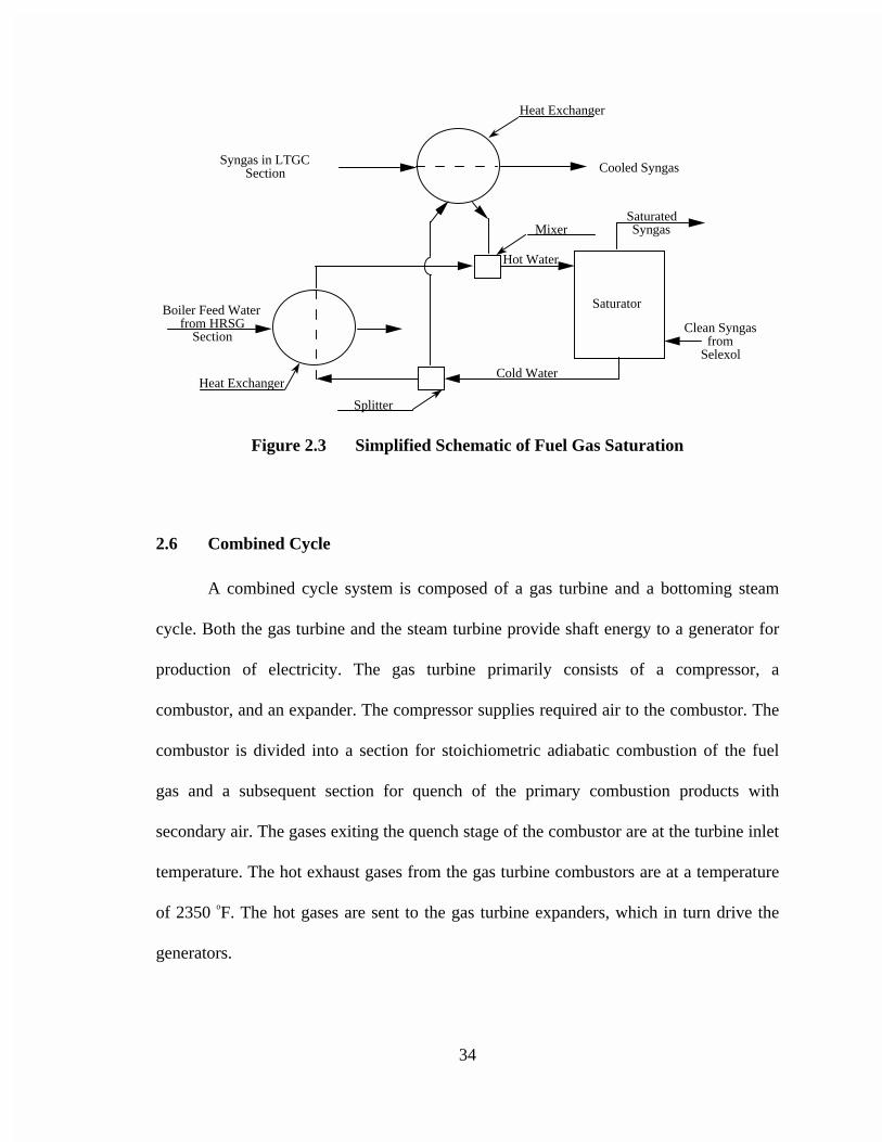
The saturation of fuel gas takes place in a saturator vessel, which is adiabatic. The
clean gas from the acid gas removal system enters the saturator from the bottom while hot
water, which is at a higher temperature than that of the syngas, is sprayed from the top of
the vessel, as shown in Figure 2.2. The typical temperature of the hot water is 380 oF,
while that of the syngas is 85 oF before saturation. The saturated gas is heated to a
temperature of approximately 350 oF and exits from the saturator from the top of the
vessel while the hot water gets cooled and exits from the bottom of the vessel. The heat
needed for heating the water is transferred from low temperature gas cooling units and the
heat recovery steam generators to the fuel gas saturation unit as shown in Figure 2.3. A
portion of the cold water leaving the fuel gas saturator is sent to heat exchangers in low
temperature gas cooling section, where it get heated while cooling the hot syngas from
the gas scrubbing section. The remaining portion of cold water is heated by heat
exchange with boiler feedwater from the heat recovery steam generation system. Both the
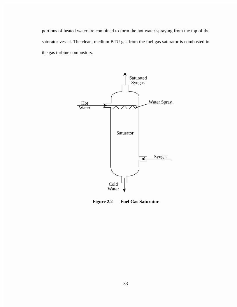
33
portions of heated water are combined to form the hot water spraying from the top of the
saturator vessel. The clean, medium BTU gas from the fuel gas saturator is combusted in
the gas turbine combustors.
Hot Water
Saturated Syngas
Cold Water
Syngas
Saturator
Water Spray
Figure 2.2 Fuel Gas Saturator
34
Syngas in LTGC Section
Heat Exchanger
Boiler Feed Water from HRSG
Section
Heat Exchanger
Saturator
Hot Water
Cold Water
Saturated Syngas
Clean Syngas from
Selexol
Cooled Syngas
Mixer
Splitter
Figure 2.3 Simplified Schematic of Fuel Gas Saturation
2.6 Combined Cycle
A combined cycle system is composed of a gas turbine and a bottoming steam
cycle. Both the gas turbine and the steam turbine provide shaft energy to a generator for
production of electricity. The gas turbine primarily consists of a compressor, a
combustor, and an expander. The compressor supplies required air to the combustor. The
combustor is divided into a section for stoichiometric adiabatic combustion of the fuel
gas and a subsequent section for quench of the primary combustion products with
secondary air. The gases exiting the quench stage of the combustor are at the turbine inlet
temperature. The hot exhaust gases from the gas turbine combustors are at a temperature
of 2350 oF. The hot gases are sent to the gas turbine expanders, which in turn drive the
generators.
35
If the gas turbine design is used for syngas as well as for natural gas, then the total
mass flow through the turbine is more or less equal in both the cases. However, the
heating value of natural gas is higher than the heating value of syngas. Therefore, the fuel
flow rate for syngas is significantly larger than that for the natural gas. Typically, the
mass flow at the turbine inlet nozzle is limited by choking. Therefore, an increase in the
fuel mass flow rate must be compensated by a reduction in the compressor air flow rate,
for a given pressure ratio and firing temperature. This causes a net reduction in the power
consumed by the compressors leading to a net increase in the gas turbine output.
The hot gas turbine exhaust gases enter the heat recovery steam generator (HRSG)
process area. The heat recovery steam generator system has gas-gas heat exchangers that
recover the sensible heat from the hot exhaust gases. The HRSG consists of a superheat
system including reheaters, high pressure evaporators, and boilers. High pressure steam is
generated in the superheat steam system using the heat recovered from the hot turbine
exhaust gases. This unit also superheats the high pressure saturated steam generated in the
high temperature gas cooling unit in the radiant and convective cooling process. The
exhaust gases that have been cooled flow out of the heat recovery steam generators at
temperatures in the range of 250 oF to 300 oF. Most of the steam generated in the HRSGs
is sent to the steam turbines where it is expanded and more electric power is generated. A
portion of steam is sent to the fuel gas saturation unit.
36
3.0 DOCUMENTATION OF THE PLANT PERFORMANCE SIMULATIONMODEL IN ASPEN OF THE COAL-FUELED TEXACO-GASIFIERBASED IGCC SYSTEM WITH RADIANT AND CONVECTIVE HIGHTEMPERATURE GAS COOLING
This chapter presents the ASPEN simulation model of the performance of an
IGCC system using a Texaco gasifier with radiant and convective high temperature gas
cooling. The details involving the modeling of the mass and energy balances of the major
process sections of the system are described. Tables and figures describing the
components of the process sections of the IGCC system model are listed in detail. The
convergence sequence, which specifies the calculation sequence of the simulation model,
is presented. Also given is a list of FORTRAN blocks and design specifications required
for the simulation model. Finally, the methods used for modeling the air pollutant
emissions from the IGCC system are discussed.
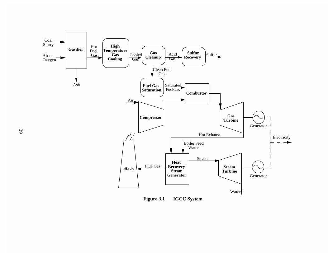
3.1 Process Description
The model of the Texaco gasifier-based IGCC system with radiant and convective
high temperature gas cooling is based primarily on the findings of a study sponsored by
the Electric Power Research Institute (Matchak et al., 1984). This study provides
extensive information on the mass flows, temperatures, and pressures of streams, power
production and consumption, and costs associated with each process section of the plant.
Thus it provides comprehensive and internally consistent information for use in model
development.
37
The model presented in this study is based upon a previous model developed by
K.R.Stone in 1985 for FETC. The modifications that were made to the previous model
include incorporation of a new and more detailed model of the gas turbine,
implementation of a fuel gas saturation model, modeling of NOX emissions, incorporation
of refined auxiliary power consumption estimates, and implementation of a capital,
annual, and levelized cost model.
The present model consists of slurry preparation units, a gasification unit, high
temperature gas cooling, particulate removal and ash removal, low temperature gas
cooling unit, fuel gas saturator and acid gas removal section, byproduct sulfur production,
and combined-cycle power system as shown in Figure 3.1. In addition to these units, the
model also incorporates auxiliary support facilities such as those that collect and treat
utility waste water.
39
Ash
Combustor
Air
Hot ExhaustElectricity
Generator
Compressor Gas Turbine
Boiler Feed Water
Steam Turbine
Water
Steam
Flue GasHeat
Recovery Steam
Generator Generator
Stack
Air or Oxygen
Clean Fuel Gas
Gas Cleanup
Gasifier
Coal Slurry Hot
Fuel Gas
High Temperature
Gas Cooling
Sulfur Recovery
Fuel Gas Saturation
SulfurAcid Gas
Saturated FuelGas
Cooled Gas
Figure 3.1 IGCC System
40
3.2 Major Process Sections in the Radiant and Convective IGCC Model
The major flowsheet sections in the process are described below. Each major
process section is referred to as a flowsheet. Within each flowsheet, unit operation
models represent specific components of that process area. There are user-specified
inputs regarding key design assumptions for each unit operation model. The numerical
values of the design assumptions are presented in this chapter. However, a user could
substitute other values for these to reflect other design alternatives.
3.2.1 Coal Slurry and Oxidant Feed to the GasifierIn this section the approach used to model slurry and oxidant feed to the gasifier is
described. The ASPEN performance simulation model accepts user input regarding the
characteristics of the coal assumed as a gasifier feedstock. The base case assumption
regarding the coal composition is given in Table 3.1 for a typical Illinois No. 6
bituminous coal. The coal is modeled as part of a coal-water slurry, such that the slurry
contains 66.5 weight percent solids.
Figure 3.2 illustrates the mass flows in the gasification process area, while Table
3.2 describes the unit operations that are modeled in this process area. The coal slurry
flows through a pump, modeled as a unit operation of the type "PUMP" with a block
identification of "SLURPUMP", to a user-defined unit operation identified as
"COALCONV". The slurry pump serves to raise the pressure of the slurry to 650 psia,
41
which is high enough for introduction into the gasifier, which operates at 615 psia in the
base case scenario. The COALCONV block serves to decompose the coal into its
constituent elements. The portions of the coal that represent soot and slag are modeled as
being removed from the coal by the blocks "MAKESLAG" and "MAKESOOT".
MAKESLAG calculates the heat required to convert a portion of the coal to slag and
MAKESOOT calculates the heat required to convert a portion of the coal to soot. Both of
the heat streams are directed to the gasifier main reactor modeled by the block
"GASIFIER". The equations used in MAKESOOT and MAKESLAG are, respectively,
SOOTASH852.0C012.0 →+ (3-1)
SLAGASH992.0C0007.0 →+ (3-2)
The oxidant feed is modeled to consist of 95 percent pure oxygen at 250 oF and
734 psia. The mass flow rate of oxidant is modeled by a design specification, SETOXYG.
SETOXYG varies the flow of oxidant such that the heat loss from the gasifier is less than
one percent of the total heat input to the gasifier. Thus, the ASPEN model calculates the
oxygen flow required to obtain the user specified gasifier outlet temperature and to
overcome this heat loss. The coal slurry and oxidant feed are mixed in the unit operation
block GASIFMIX and sent to the gasification unit modeled by the equilibrium reactor
unit operation block GASIFIER.
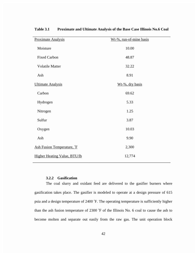
42
Table 3.1 Proximate and Ultimate Analysis of the Base Case Illinois No.6 Coal
Proximate Analysis Wt-%, run-of-mine basis
Moisture 10.00
Fixed Carbon 48.87
Volatile Matter 32.22
Ash 8.91
Ultimate Analysis Wt-%, dry basis
Carbon 69.62
Hydrogen 5.33
Nitrogen 1.25
Sulfur 3.87
Oxygen 10.03
Ash 9.90
Ash Fusion Temperature, oF 2,300
Higher Heating Value, BTU/lb 12,774
3.2.2 GasificationThe coal slurry and oxidant feed are delivered to the gasifier burners where
gasification takes place. The gasifier is modeled to operate at a design pressure of 615
psia and a design temperature of 2400 oF. The operating temperature is sufficiently higher
than the ash fusion temperature of 2300 oF of the Illinois No. 6 coal to cause the ash to
become molten and separate out easily from the raw gas. The unit operation block
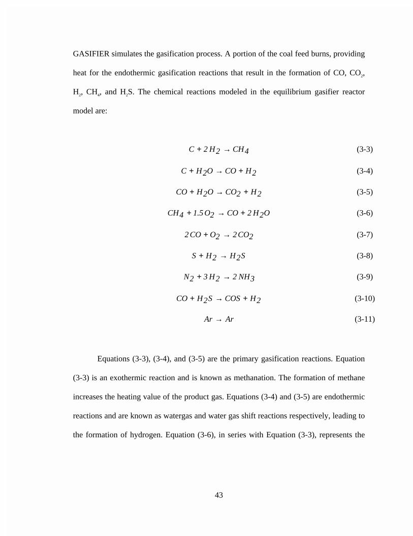
43
GASIFIER simulates the gasification process. A portion of the coal feed burns, providing
heat for the endothermic gasification reactions that result in the formation of CO, CO2,
H2, CH4, and H2S. The chemical reactions modeled in the equilibrium gasifier reactor
model are:
4CH2H2C →+ (3-3)
2HCOO2HC +→+ (3-4)
2H2COO2HCO +→+ (3-5)
O2H2CO2O5.14CH +→+ (3-6)
2CO22OCO2 →+ (3-7)
S2H2HS →+ (3-8)
3NH22H32N →+ (3-9)
2HCOSS2HCO +→+ (3-10)
ArAr → (3-11)
Equations (3-3), (3-4), and (3-5) are the primary gasification reactions. Equation
(3-3) is an exothermic reaction and is known as methanation. The formation of methane
increases the heating value of the product gas. Equations (3-4) and (3-5) are endothermic
reactions and are known as watergas and water gas shift reactions respectively, leading to
the formation of hydrogen. Equation (3-6), in series with Equation (3-3), represents the

44
partial combustion of coal and Equation (3-7) in sequence with Equations (3-3) and (3-4),
models the complete oxidation of coal.
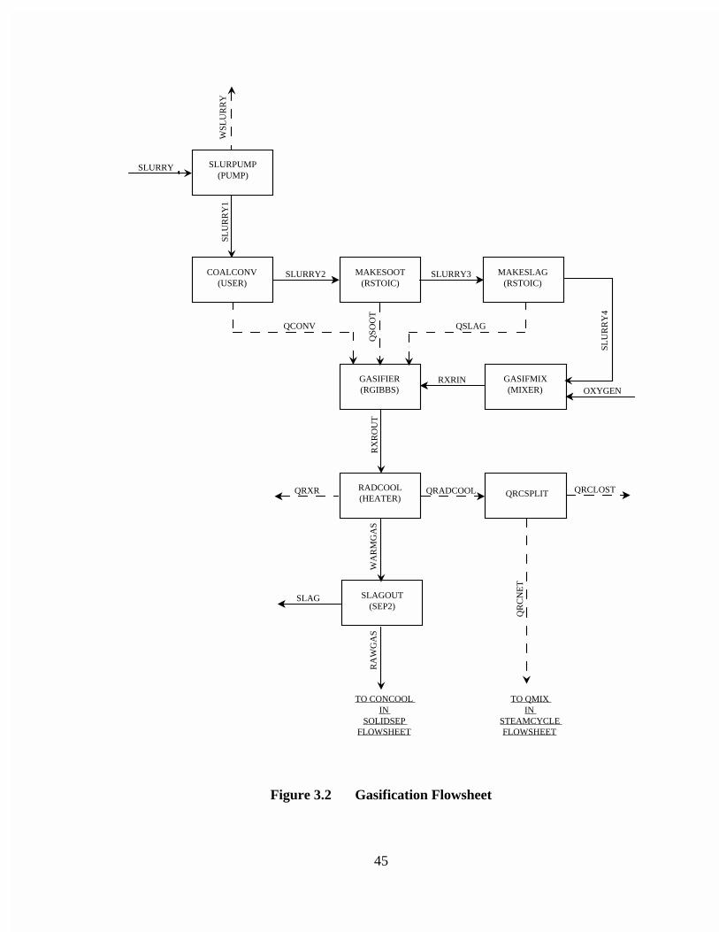
45
SLURPUMP (PUMP)
COALCONV (USER)
MAKESOOT (RSTOIC)
MAKESLAG (RSTOIC)
GASIFIER (RGIBBS)
GASIFMIX (MIXER)
RADCOOL (HEATER) QRCSPLIT
SLAGOUT (SEP2)
TO CONCOOL IN
SOLIDSEP FLOWSHEET
TO QMIX IN
STEAMCYCLE FLOWSHEET
SLURRY
WSL
UR
RY
SLU
RR
Y1
SLURRY2 SLURRY3
SLU
RR
Y4
QCONV
QSO
OT
QSLAG
QRADCOOL QRCLOST
OXYGENRXRIN
RX
RO
UT
QRXR
WA
RM
GA
S
QR
CN
ET
SLAG
RA
WG
AS
Figure 3.2 Gasification Flowsheet
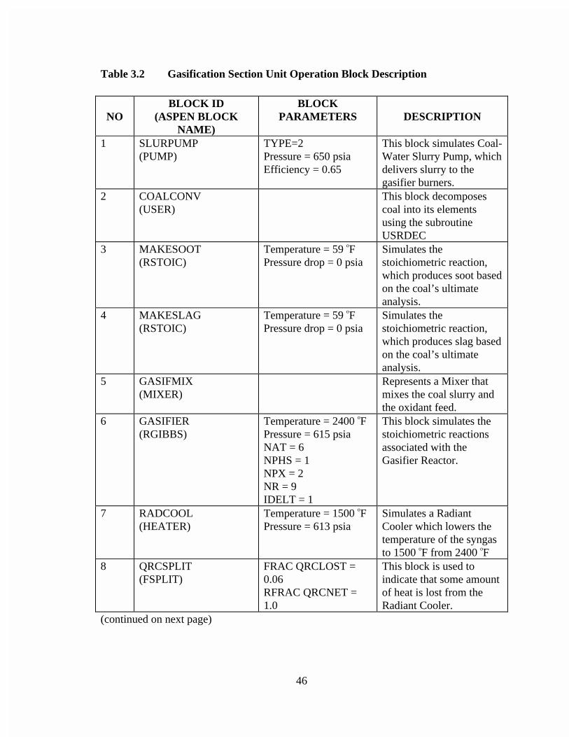
46
Table 3.2 Gasification Section Unit Operation Block Description
NOBLOCK ID
(ASPEN BLOCKNAME)
BLOCKPARAMETERS DESCRIPTION
1 SLURPUMP(PUMP)
TYPE=2Pressure = 650 psiaEfficiency = 0.65
This block simulates Coal-Water Slurry Pump, whichdelivers slurry to thegasifier burners.
2 COALCONV(USER)
This block decomposescoal into its elementsusing the subroutineUSRDEC
3 MAKESOOT(RSTOIC)
Temperature = 59 oFPressure drop = 0 psia
Simulates thestoichiometric reaction,which produces soot basedon the coal’s ultimateanalysis.
4 MAKESLAG(RSTOIC)
Temperature = 59 oFPressure drop = 0 psia
Simulates thestoichiometric reaction,which produces slag basedon the coal’s ultimateanalysis.
5 GASIFMIX(MIXER)
Represents a Mixer thatmixes the coal slurry andthe oxidant feed.
6 GASIFIER(RGIBBS)
Temperature = 2400 oFPressure = 615 psiaNAT = 6NPHS = 1NPX = 2NR = 9IDELT = 1
This block simulates thestoichiometric reactionsassociated with theGasifier Reactor.
7 RADCOOL(HEATER)
Temperature = 1500 oFPressure = 613 psia
Simulates a RadiantCooler which lowers thetemperature of the syngasto 1500 oF from 2400 oF
8 QRCSPLIT(FSPLIT)
FRAC QRCLOST =0.06RFRAC QRCNET =1.0
This block is used toindicate that some amountof heat is lost from theRadiant Cooler.
(continued on next page)
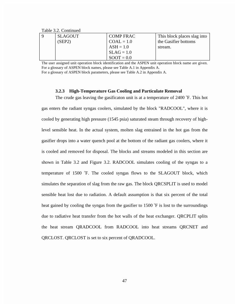
47
Table 3.2. Continued9 SLAGOUT
(SEP2)COMP FRACCOAL = 1.0ASH = 1.0SLAG = 1.0SOOT = 0.0
This block places slag intothe Gasifier bottomsstream.
The user assigned unit operation block identification and the ASPEN unit operation block name are given.For a glossary of ASPEN block names, please see Table A.1 in Appendix A.For a glossary of ASPEN block parameters, please see Table A.2 in Appendix A.
3.2.3 High-Temperature Gas Cooling and Particulate RemovalThe crude gas leaving the gasificaton unit is at a temperature of 2400 oF. This hot
gas enters the radiant syngas coolers, simulated by the block "RADCOOL", where it is
cooled by generating high pressure (1545 psia) saturated steam through recovery of high-
level sensible heat. In the actual system, molten slag entrained in the hot gas from the
gasifier drops into a water quench pool at the bottom of the radiant gas coolers, where it
is cooled and removed for disposal. The blocks and streams modeled in this section are
shown in Table 3.2 and Figure 3.2. RADCOOL simulates cooling of the syngas to a
temperature of 1500 oF. The cooled syngas flows to the SLAGOUT block, which
simulates the separation of slag from the raw gas. The block QRCSPLIT is used to model
sensible heat lost due to radiation. A default assumption is that six percent of the total
heat gained by cooling the syngas from the gasifier to 1500 oF is lost to the surroundings
due to radiative heat transfer from the hot walls of the heat exchanger. QRCPLIT splits
the heat stream QRADCOOL from RADCOOL into heat streams QRCNET and
QRCLOST. QRCLOST is set to six percent of QRADCOOL.
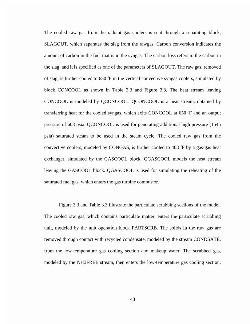
48
The cooled raw gas from the radiant gas coolers is sent through a separating block,
SLAGOUT, which separates the slag from the rawgas. Carbon conversion indicates the
amount of carbon in the fuel that is in the syngas. The carbon loss refers to the carbon in
the slag, and it is specified as one of the parameters of SLAGOUT. The raw gas, removed
of slag, is further cooled to 650 oF in the vertical convective syngas coolers, simulated by
block CONCOOL as shown in Table 3.3 and Figure 3.3. The heat stream leaving
CONCOOL is modeled by QCONCOOL. QCONCOOL is a heat stream, obtained by
transferring heat for the cooled syngas, which exits CONCOOL at 650 oF and an output
pressure of 603 psia. QCONCOOL is used for generating additional high pressure (1545
psia) saturated steam to be used in the steam cycle. The cooled raw gas from the
convective coolers, modeled by CONGAS, is further cooled to 403 oF by a gas-gas heat
exchanger, simulated by the GASCOOL block. QGASCOOL models the heat stream
leaving the GASCOOL block. QGASCOOL is used for simulating the reheating of the
saturated fuel gas, which enters the gas turbine combustor.
Figure 3.3 and Table 3.3 illustrate the particulate scrubbing sections of the model.
The cooled raw gas, which contains particulate matter, enters the particulate scrubbing
unit, modeled by the unit operation block PARTSCRB. The solids in the raw gas are
removed through contact with recycled condensate, modeled by the stream CONDSATE,
from the low-temperature gas cooling section and makeup water. The scrubbed gas,
modeled by the NH3FREE stream, then enters the low-temperature gas cooling section.
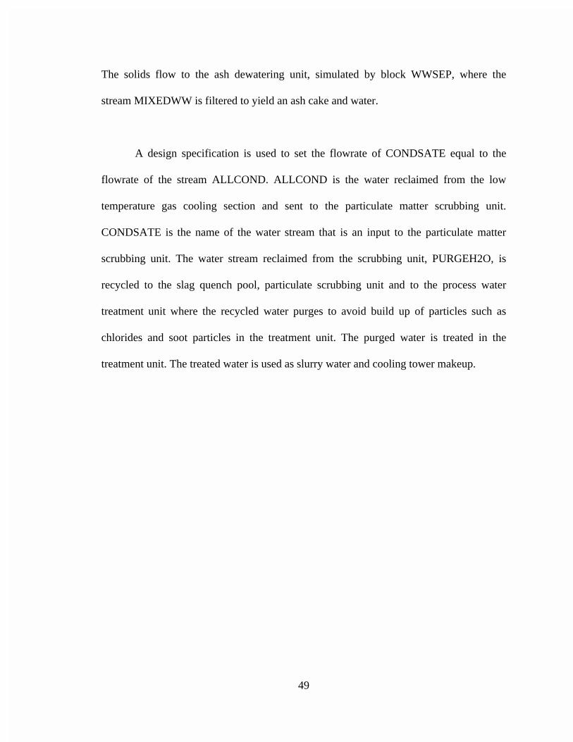
49
The solids flow to the ash dewatering unit, simulated by block WWSEP, where the
stream MIXEDWW is filtered to yield an ash cake and water.
A design specification is used to set the flowrate of CONDSATE equal to the
flowrate of the stream ALLCOND. ALLCOND is the water reclaimed from the low
temperature gas cooling section and sent to the particulate matter scrubbing unit.
CONDSATE is the name of the water stream that is an input to the particulate matter
scrubbing unit. The water stream reclaimed from the scrubbing unit, PURGEH2O, is
recycled to the slag quench pool, particulate scrubbing unit and to the process water
treatment unit where the recycled water purges to avoid build up of particles such as
chlorides and soot particles in the treatment unit. The purged water is treated in the
treatment unit. The treated water is used as slurry water and cooling tower makeup.
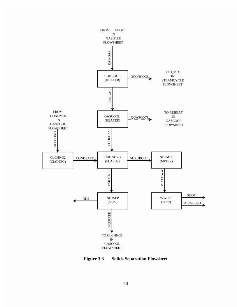
50
CONCOOL (HEATER)
GASCOOL (HEATER)
CLCHNG2 (CLCHNG)
PARTSCRB (FLASH2)
NH3SEP (SEP2)
NH3MIX (MIXER)
WWSEP (SEP2)
FROM CONDMIX
IN GASCOOL
FLOWSHEET
TO CLCHNG1 IN
GASCOOL FLOWSHEET
TO QMIX IN
STEAMCYCLE FLOWSHEET
FROM SLAGOUT IN
GASIFIER FLOWSHEET
RA
WG
AS
CO
NG
AS
QCONCOOL
QGASCOOL
CO
OL
GA
S
CONDSATE
AL
LC
ON
D
PAR
TFR
EE
NH
3FR
EE
MIX
ED
WW
SCRUBOUT
TO REHEAT IN
GASCOOL FLOWSHEET
SOOT
PURGEH2ONH3
Figure 3.3 Solids Separation Flowsheet
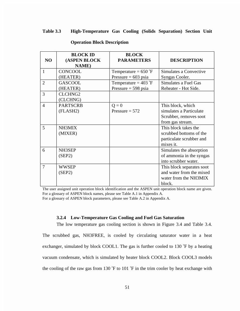
51
Table 3.3 High-Temperature Gas Cooling (Solids Separation) Section Unit
Operation Block Description
NOBLOCK ID
(ASPEN BLOCKNAME)
BLOCKPARAMETERS DESCRIPTION
1 CONCOOL(HEATER)
Temperature = 650 oFPressure = 603 psia
Simulates a ConvectiveSyngas Cooler.
2 GASCOOL(HEATER)
Temperature = 403 oFPressure = 598 psia
Simulates a Fuel GasReheater - Hot Side.
3 CLCHNG2(CLCHNG)
4 PARTSCRB(FLASH2)
Q = 0Pressure = 572
This block, whichsimulates a ParticulateScrubber, removes sootfrom gas stream.
5 NH3MIX(MIXER)
This block takes thescrubbed bottoms of theparticulate scrubber andmixes it.
6 NH3SEP(SEP2)
Simulates the absorptionof ammonia in the syngasinto scrubber water.
7 WWSEP(SEP2)
This block separates sootand water from the mixedwater from the NH3MIXblock.
The user assigned unit operation block identification and the ASPEN unit operation block name are given.For a glossary of ASPEN block names, please see Table A.1 in Appendix A.For a glossary of ASPEN block parameters, please see Table A.2 in Appendix A.
3.2.4 Low-Temperature Gas Cooling and Fuel Gas SaturationThe low temperature gas cooling section is shown in Figure 3.4 and Table 3.4.
The scrubbed gas, NH3FREE, is cooled by circulating saturator water in a heat
exchanger, simulated by block COOL1. The gas is further cooled to 130 oF by a heating
vacuum condensate, which is simulated by heater block COOL2. Block COOL3 models
the cooling of the raw gas from 130 oF to 101 oF in the trim cooler by heat exchange with
52
cooling water. The condensate from the heat exchangers is collected in the condensate
collection drum, the latter of which is simulated by mixer block CONDMIX. The cooled
gas, stream COLDGAS, is sent to the Selexol acid gas removal unit.
The Selexol unit separates the stream COLDGAS into streams CLEANGAS,
ACIDGAS, and FLASHGAS. ACIDGAS, containing 97.6 percent of H2S by volume is
sent to the mixer, CLAUSMIX, in the Claus plant. The stream FLASHGAS is sent to the
mixer, BSMIX, in the Beavon-Stretford tail gas treatment plant.
The clean gas from the Selexol process, modeled by the stream CLEANGAS,
enters the saturation unit at 85 oF and 429 psia. The details of the modeling of the fuel gas
saturation unit are shown in Figure 3.5 and Table 3.4. The required amount of water to be
added to clean gas to make its moisture content 28.2 % by weight is calculated by a
FORTRAN block SATURH2O. SATURH2O obtains the mass flow of clean gas entering
the saturator block and calculates the required saturated fuel gas mass flow, modeled by
the stream SATGAS. SATGAS is required to be at a temperature of 347 oF which is
achieved by using a design specification SETSATR. SETSATR calculates the required
amount of hot water entering the saturation unit through the block FAKESPLT. This
block splits the hot water stream, HOTH2O into HOTH21 and SATCOM streams.
HOTH21 is cooled by a heat exchanger, FAKECOOL, to a temperature of 235 oF.
SATCOM and CLEANGAS enter FAKEMIX, which simulates a mixer. The saturated
fuel gas from FAKEMIX, SATGAS1, is heated to the required temperature of 347 oF in
53
the block FAKEHEAT by QHEATS, the heat stream leaving FAKECOOL. As shown in
Figure 2.3, the required amount of circulating water to the saturation unit is maintained
by heating the circulating water in heat exchanger COOL1. A slip stream of high pressure
boiler feed water (BFW) is used to supply the necessary heat to the circulating water
coming out of GASCOOL. The slipstream BFW, the circulating water from GASCOOL
and COOL1 combine to form the hot water, HOTH2O which enters the block
FAKESPLT. The fuel gas exits the saturator at 347 oF with a moisture content of 28.2
weight percent and is reheated to 570 oF in the block REHEAT with the help of the heat
stream QGASCOOL from the high temperature gas cooling section. The reheated fuel
gas, the stream GTFUEL, flows to the gas turbine combustors.
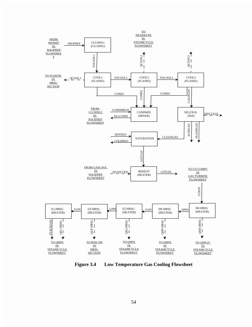
54
CLCHNG1 (CLCHNG)
COOL1 (FLASH2)
COOL2 (FLASH2)
COOL3 (FLASH2)
CONDMIX (MIXER)
REHEAT (HEATER)
SELEXOL (SEP)
E1-HRSG (HEATER)
E2-HRSG (HEATER)
LP-HRSG (HEATER)
HP-HRSG (HEATER)
SH-HRSG (HEATER)
FROM NH3SEP
IN SOLIDSEP
FLOWSHEET
TO FGSHTR IN
HRSG SECTION
FROM CLCHNG2
IN SOLIDSEP
FLOWSHEET
FROM GASCOOL IN
SOLIDSEP FLOWSHEET
TO GT-COMP1 IN
GAS TURBINE FLOWSHEET
TO QSPLIT IN
STEAMCYCLE FLOWSHEET
TO QMIX IN
STEAMCYCLE FLOWSHEET
TO QMIX IN
STEAMCYCLE FLOWSHEET
TO QMIX IN
STEAMCYCLE FLOWSHEET
TO BOIL100 IN
HRSG SECTION
NH3FREE
QCOOL1 TOCOOL2 TOCOOL3
COND1 COND3
CO
ND
2Q
CO
OL
2
CO
LD
GA
S
CONDMKUP
ALLCOND
CLEANGAS
QSELEXOL
AC
IDG
AS
FL
AS
HG
AS
QGASCOOL GTFUEL
HPINE2IN
GT
POC
LPINE1IN
ST
AC
KG
AS
QE
1-H
RS
G
QL
P-H
RS
G
QE
2-H
RS
G
QH
P-H
RS
G
QS
H-H
RS
G
TO DEAERATR
IN STEAMCYCLE FLOWSHEET
TO
CO
OL
1
SA
TG
AS
QC
OO
L3
SATURATIONHOTH2O
COLDH2O
Figure 3.4 Low Temperature Gas Cooling Flowsheet
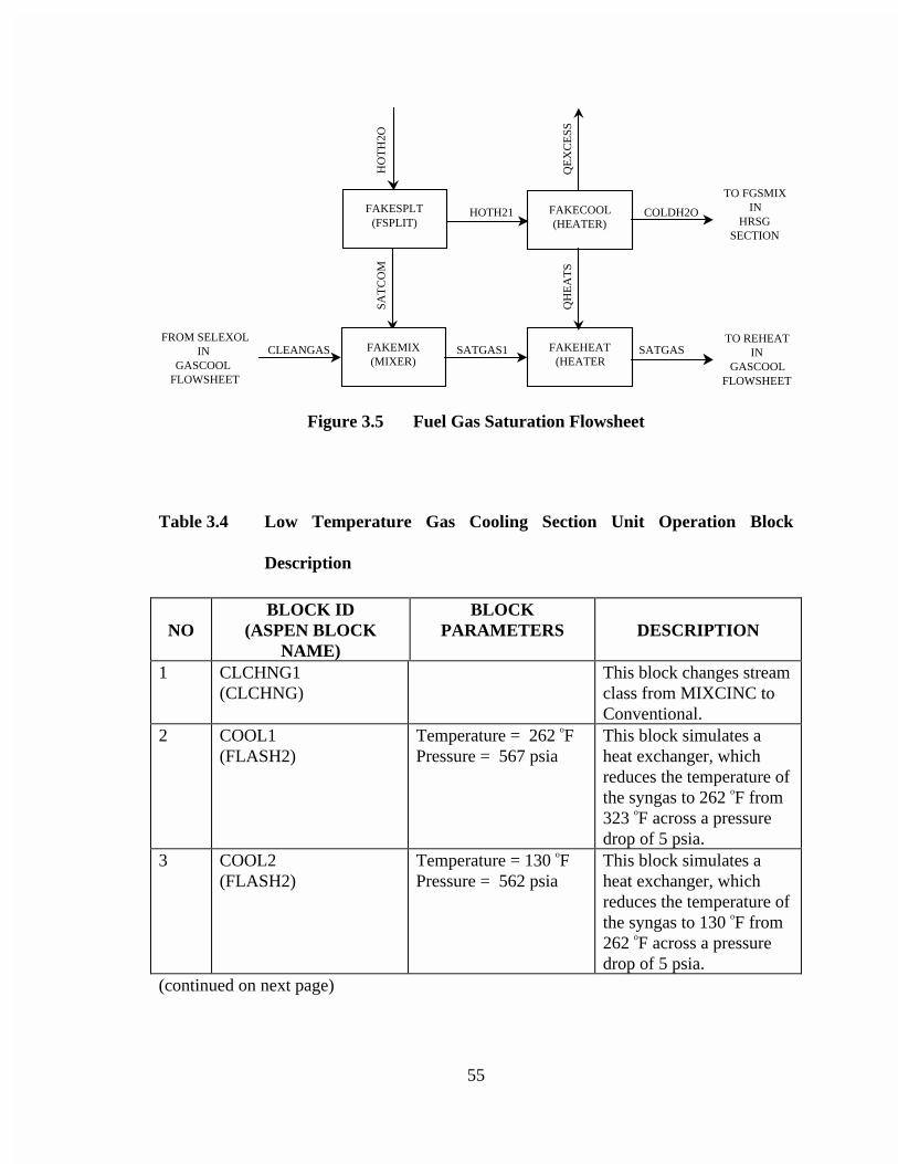
55
FAKESPLT (FSPLIT)
HO
TH
2O
FAKECOOL (HEATER)
FAKEMIX (MIXER)
HOTH21
SA
TC
OM
FAKEHEAT (HEATER
SATGAS1
COLDH2O
CLEANGAS
QH
EA
TS
SATGAS
QE
XC
ESS
FROM SELEXOL IN
GASCOOL FLOWSHEET
TO REHEAT IN
GASCOOL FLOWSHEET
TO FGSMIX IN
HRSG SECTION
Figure 3.5 Fuel Gas Saturation Flowsheet
Table 3.4 Low Temperature Gas Cooling Section Unit Operation Block
Description
NOBLOCK ID
(ASPEN BLOCKNAME)
BLOCKPARAMETERS DESCRIPTION
1 CLCHNG1(CLCHNG)
This block changes streamclass from MIXCINC toConventional.
2 COOL1(FLASH2)
Temperature = 262 oFPressure = 567 psia
This block simulates aheat exchanger, whichreduces the temperature ofthe syngas to 262 oF from323 oF across a pressuredrop of 5 psia.
3 COOL2(FLASH2)
Temperature = 130 oFPressure = 562 psia
This block simulates aheat exchanger, whichreduces the temperature ofthe syngas to 130 oF from262 oF across a pressuredrop of 5 psia.
(continued on next page)
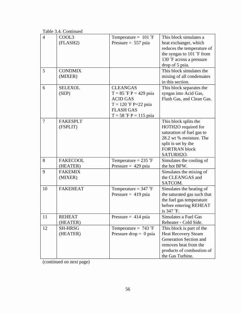
56
Table 3.4. Continued4 COOL3
(FLASH2)Temperature = 101 oFPressure = 557 psia
This block simulates aheat exchanger, whichreduces the temperature ofthe syngas to 101 oF from130 oF across a pressuredrop of 5 psia.
5 CONDMIX(MIXER)
This block simulates themixing of all condensatesin this section.
6 SELEXOL(SEP)
CLEANGAST = 85 oF P = 429 psiaACID GAST = 120 oF P=22 psiaFLASH GAST = 58 oF P = 115 psia
This block separates thesyngas into Acid Gas,Flash Gas, and Clean Gas.
7 FAKESPLT(FSPLIT)
This block splits theHOTH2O required forsaturation of fuel gas to28.2 wt % moisture. Thesplit is set by theFORTRAN blockSATURH2O.
8 FAKECOOL(HEATER)
Temperature = 235 oFPressure = 429 psia
Simulates the cooling ofthe hot BFW.
9 FAKEMIX(MIXER)
Simulates the mixing ofthe CLEANGAS andSATCOM.
10 FAKEHEAT Temperature = 347 oFPressure = 419 psia
Simulates the heating ofthe saturated gas such thatthe fuel gas temperaturebefore entering REHEATis 347 oF.
11 REHEAT(HEATER)
Pressure = 414 psia Simulates a Fuel GasReheater - Cold Side.
12 SH-HRSG(HEATER)
Temperature = 743 oFPressure drop = 0 psia
This block is part of theHeat Recovery SteamGeneration Section andremoves heat from theproducts of combustion ofthe Gas Turbine.
(continued on next page)
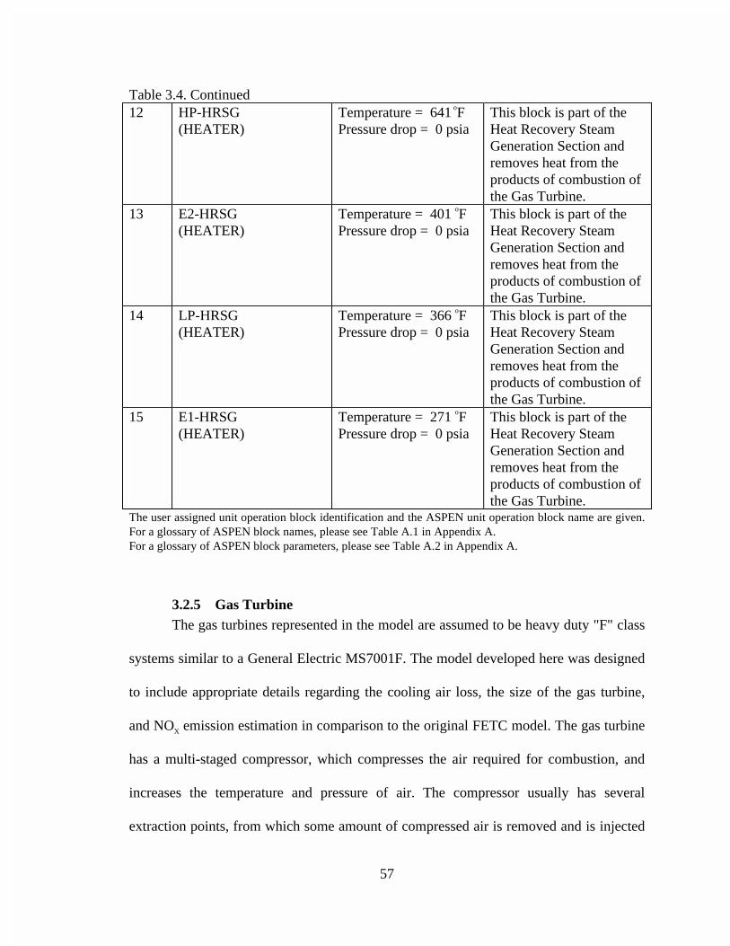
57
Table 3.4. Continued12 HP-HRSG
(HEATER)Temperature = 641 oFPressure drop = 0 psia
This block is part of theHeat Recovery SteamGeneration Section andremoves heat from theproducts of combustion ofthe Gas Turbine.
13 E2-HRSG(HEATER)
Temperature = 401 oFPressure drop = 0 psia
This block is part of theHeat Recovery SteamGeneration Section andremoves heat from theproducts of combustion ofthe Gas Turbine.
14 LP-HRSG(HEATER)
Temperature = 366 oFPressure drop = 0 psia
This block is part of theHeat Recovery SteamGeneration Section andremoves heat from theproducts of combustion ofthe Gas Turbine.
15 E1-HRSG(HEATER)
Temperature = 271 oFPressure drop = 0 psia
This block is part of theHeat Recovery SteamGeneration Section andremoves heat from theproducts of combustion ofthe Gas Turbine.
The user assigned unit operation block identification and the ASPEN unit operation block name are given.For a glossary of ASPEN block names, please see Table A.1 in Appendix A.For a glossary of ASPEN block parameters, please see Table A.2 in Appendix A.
3.2.5 Gas TurbineThe gas turbines represented in the model are assumed to be heavy duty "F" class
systems similar to a General Electric MS7001F. The model developed here was designed
to include appropriate details regarding the cooling air loss, the size of the gas turbine,
and NOX emission estimation in comparison to the original FETC model. The gas turbine
has a multi-staged compressor, which compresses the air required for combustion, and
increases the temperature and pressure of air. The compressor usually has several
extraction points, from which some amount of compressed air is removed and is injected
58
into the blades and vanes of the hottest turbine stages in order to cool the blades and
vanes. The gas turbine combustor receives the syngas and the compressed air and
combusts them. The hot exhaust gases are expanded in the turbine in several stages,
represented in the model by three expanders.
3.2.5.1 Compression
Ambient conditions of the atmospheric air entering the gas turbine compressor are
assumed to be 59 oF, 14.7 psia, and 60 percent relative humidity. These values are taken
as defaults and can be changed by the user. The default compressor ratio is assumed to be
15.5, which is typical of heavy duty gas turbines (Farmer, 1997), resulting in a
compressor outlet pressure of 227.85 psia. Figure 3.6 and Table 3.5 present the gas
turbine model in detail.
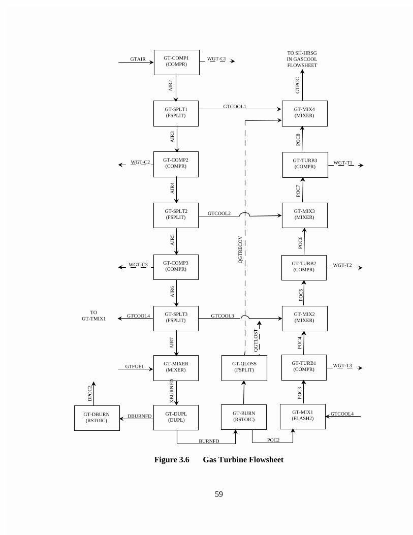
59
GT-COMP1 (COMPR)
GT-COMP2 (COMPR)
GT-COMP3 (COMPR)
GT-TURB1 (COMPR)
GT-TURB2 (COMPR)
GT-TURB3 (COMPR)
GT-SPLT1 (FSPLIT)
GT-SPLT2 (FSPLIT)
GT-SPLT3 (FSPLIT)
GT-QLOSS (FSPLIT)
GT-MIX1 (FLASH2)
GT-MIX2 (MIXER)
GT-MIX3 (MIXER)
GT-MIX4 (MIXER)
GT-MIXER (MIXER)
GT-BURN (RSTOIC)
GT-DBURN (RSTOIC)
GT-DUPL (DUPL)
GTAIR
AIR
3A
IR2
AIR
4A
IR5
AIR
6A
IR7
GTFUEL
WGT-C1
WGT-C2
GTCOOL1
GTCOOL2
WGT-C3
GTCOOL3GTCOOL4
XB
UR
NFD
BURNFD
DBURNFD
DPO
C2
QG
TL
OST
QG
TR
EC
OV
POC2
POC
3PO
C4
POC
5PO
C6
POC
7PO
C8
WGT-T1
WGT-T2
WGT-T3
GT
POC
TO GT-TMIX1
GTCOOL4
TO SH-HRSG IN GASCOOL FLOWSHEET
Figure 3.6 Gas Turbine Flowsheet
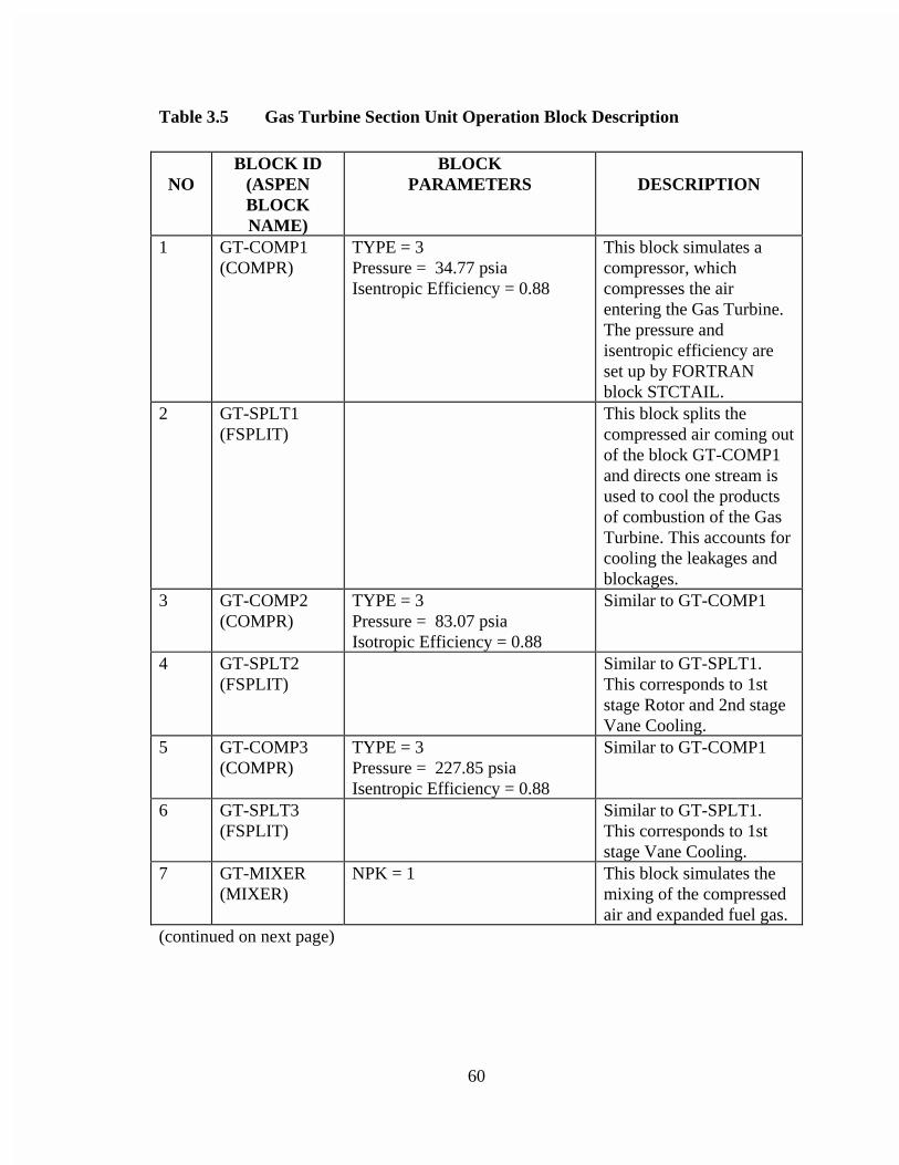
60
Table 3.5 Gas Turbine Section Unit Operation Block Description
NOBLOCK ID
(ASPENBLOCKNAME)
BLOCKPARAMETERS DESCRIPTION
1 GT-COMP1(COMPR)
TYPE = 3Pressure = 34.77 psiaIsentropic Efficiency = 0.88
This block simulates acompressor, whichcompresses the airentering the Gas Turbine.The pressure andisentropic efficiency areset up by FORTRANblock STCTAIL.
2 GT-SPLT1(FSPLIT)
This block splits thecompressed air coming outof the block GT-COMP1and directs one stream isused to cool the productsof combustion of the GasTurbine. This accounts forcooling the leakages andblockages.
3 GT-COMP2(COMPR)
TYPE = 3Pressure = 83.07 psiaIsotropic Efficiency = 0.88
Similar to GT-COMP1
4 GT-SPLT2(FSPLIT)
Similar to GT-SPLT1.This corresponds to 1ststage Rotor and 2nd stageVane Cooling.
5 GT-COMP3(COMPR)
TYPE = 3Pressure = 227.85 psiaIsentropic Efficiency = 0.88
Similar to GT-COMP1
6 GT-SPLT3(FSPLIT)
Similar to GT-SPLT1.This corresponds to 1ststage Vane Cooling.
7 GT-MIXER(MIXER)
NPK = 1 This block simulates themixing of the compressedair and expanded fuel gas.
(continued on next page)
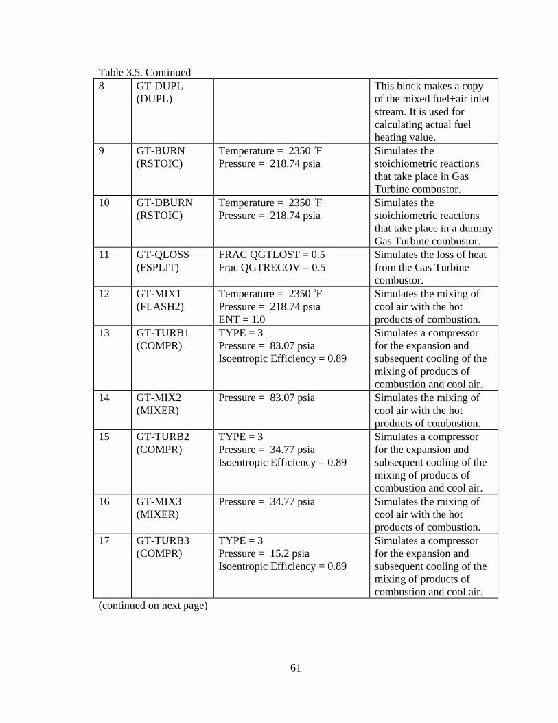
61
Table 3.5. Continued8 GT-DUPL
(DUPL)This block makes a copyof the mixed fuel+air inletstream. It is used forcalculating actual fuelheating value.
9 GT-BURN(RSTOIC)
Temperature = 2350 oFPressure = 218.74 psia
Simulates thestoichiometric reactionsthat take place in GasTurbine combustor.
10 GT-DBURN(RSTOIC)
Temperature = 2350 oFPressure = 218.74 psia
Simulates thestoichiometric reactionsthat take place in a dummyGas Turbine combustor.
11 GT-QLOSS(FSPLIT)
FRAC QGTLOST = 0.5Frac QGTRECOV = 0.5
Simulates the loss of heatfrom the Gas Turbinecombustor.
12 GT-MIX1(FLASH2)
Temperature = 2350 oFPressure = 218.74 psiaENT = 1.0
Simulates the mixing ofcool air with the hotproducts of combustion.
13 GT-TURB1(COMPR)
TYPE = 3Pressure = 83.07 psiaIsoentropic Efficiency = 0.89
Simulates a compressorfor the expansion andsubsequent cooling of themixing of products ofcombustion and cool air.
14 GT-MIX2(MIXER)
Pressure = 83.07 psia Simulates the mixing ofcool air with the hotproducts of combustion.
15 GT-TURB2(COMPR)
TYPE = 3Pressure = 34.77 psiaIsoentropic Efficiency = 0.89
Simulates a compressorfor the expansion andsubsequent cooling of themixing of products ofcombustion and cool air.
16 GT-MIX3(MIXER)
Pressure = 34.77 psia Simulates the mixing ofcool air with the hotproducts of combustion.
17 GT-TURB3(COMPR)
TYPE = 3Pressure = 15.2 psiaIsoentropic Efficiency = 0.89
Simulates a compressorfor the expansion andsubsequent cooling of themixing of products ofcombustion and cool air.
(continued on next page)
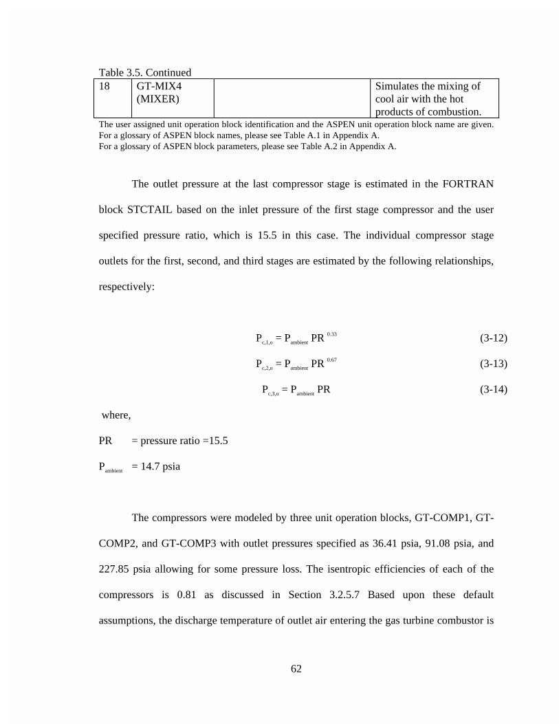
62
Table 3.5. Continued18 GT-MIX4
(MIXER)Simulates the mixing ofcool air with the hotproducts of combustion.
The user assigned unit operation block identification and the ASPEN unit operation block name are given.For a glossary of ASPEN block names, please see Table A.1 in Appendix A.For a glossary of ASPEN block parameters, please see Table A.2 in Appendix A.
The outlet pressure at the last compressor stage is estimated in the FORTRAN
block STCTAIL based on the inlet pressure of the first stage compressor and the user
specified pressure ratio, which is 15.5 in this case. The individual compressor stage
outlets for the first, second, and third stages are estimated by the following relationships,
respectively:
Pc,1,o = Pambient PR 0.33 (3-12)
Pc,2,o = Pambient PR 0.67 (3-13)
Pc,3,o = Pambient PR (3-14)
where,
PR = pressure ratio =15.5
Pambient = 14.7 psia
The compressors were modeled by three unit operation blocks, GT-COMP1, GT-
COMP2, and GT-COMP3 with outlet pressures specified as 36.41 psia, 91.08 psia, and
227.85 psia allowing for some pressure loss. The isentropic efficiencies of each of the
compressors is 0.81 as discussed in Section 3.2.5.7 Based upon these default
assumptions, the discharge temperature of outlet air entering the gas turbine combustor is
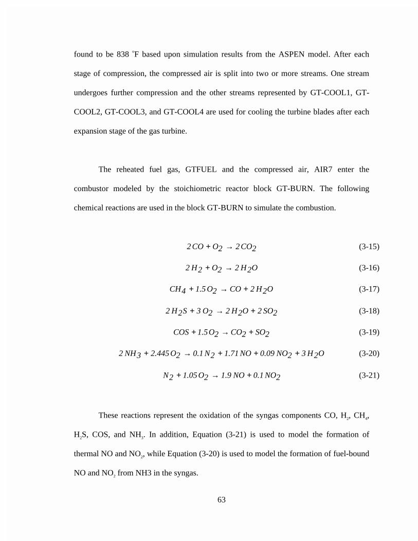
63
found to be 838 oF based upon simulation results from the ASPEN model. After each
stage of compression, the compressed air is split into two or more streams. One stream
undergoes further compression and the other streams represented by GT-COOL1, GT-
COOL2, GT-COOL3, and GT-COOL4 are used for cooling the turbine blades after each
expansion stage of the gas turbine.
The reheated fuel gas, GTFUEL and the compressed air, AIR7 enter the
combustor modeled by the stoichiometric reactor block GT-BURN. The following
chemical reactions are used in the block GT-BURN to simulate the combustion.
2CO22OCO2 →+ (3-15)
O2H22O2H2 →+ (3-16)
O2H2CO2O5.14CH +→+ (3-17)
2SO2O2H22O3S2H2 +→+ (3-18)
2SO2CO2O5.1COS +→+ (3-19)
O2H32NO09.0NO71.12N1.02O445.23NH2 +++→+ (3-20)
2NO1.0NO9.12O05.12N +→+ (3-21)
These reactions represent the oxidation of the syngas components CO, H2, CH4,
H2S, COS, and NH3. In addition, Equation (3-21) is used to model the formation of
thermal NO and NO2, while Equation (3-20) is used to model the formation of fuel-bound
NO and NO2 from NH3 in the syngas.
64
The firing temperature of a gas turbine is the temperature at which combustion
process takes place in the combustor. The higher the firing temperature, the higher the
temperature of the hot gases entering the turbine. The firing temperature of the gas
turbine is constrained by the requirement that the turbine exhaust gas, GTPOC, has a
temperature of 1120 oF or less to prevent damage to the turbine blades (Farmer, 1997).
This constraint is met using a design specification, SETHRST, which is described Section
3.2.5.6.
The expansion of the hot products of combustion, stream POC2, leaving the
combustor is modeled in three stages. Each of the three stages consist of a turbine, which
are modeled by GT-TURB1, GT-TURB2, and GT-TURB3 and a mixer, which are
modeled by GT-MIX1, GT-MIX2, GT-MIX3. In each of these stages, the hot gases are
mixed with the cooler air coming from one of the blocks GT-SPLT1, GT-SPLT2, or GT-
SPLT3 and then expanded in the turbine. The first, second, and third turbines have an
outlet pressures of 91.08 psia, 36.41 psia, and 15.42 psia, respectively, and each has an
isentropic efficiency of 0.919. The exhaust gases, GTPOC, enter the heat recovery steam
generation (HRSG) unit.
The outlet pressure at each expander stage is estimated in FORTRAN block
STCTAIL using the same method used for compression stages.
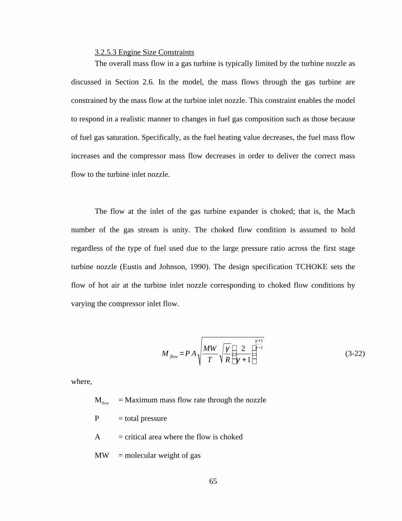
65
3.2.5.3 Engine Size Constraints
The overall mass flow in a gas turbine is typically limited by the turbine nozzle as
discussed in Section 2.6. In the model, the mass flows through the gas turbine are
constrained by the mass flow at the turbine inlet nozzle. This constraint enables the model
to respond in a realistic manner to changes in fuel gas composition such as those because
of fuel gas saturation. Specifically, as the fuel heating value decreases, the fuel mass flow
increases and the compressor mass flow decreases in order to deliver the correct mass
flow to the turbine inlet nozzle.
The flow at the inlet of the gas turbine expander is choked; that is, the Mach
number of the gas stream is unity. The choked flow condition is assumed to hold
regardless of the type of fuel used due to the large pressure ratio across the first stage
turbine nozzle (Eustis and Johnson, 1990). The design specification TCHOKE sets the
flow of hot air at the turbine inlet nozzle corresponding to choked flow conditions by
varying the compressor inlet flow.
1
1
1
2 −+
+
=γγ
γγRT
MWAPM flow (3-22)
where,
Mflow = Maximum mass flow rate through the nozzle
P = total pressure
A = critical area where the flow is choked
MW = molecular weight of gas
66
T = total temperature
R = universal gas constant
γ = ratio of specific heats for the gas
The mass flow rate of the ambient air entering the gas turbine combustor is
initialized in the ASPEN input file. The mass flow rate of the ambient air is adjusted by
TCHOKE to achieve a specified turbine nozzle gas mass flow rate. The choked mass flow
is calculated based on a reference mass flow, adjusted for differences in pressure,
temperature, and molecular weight, and assuming that the critical area and ratio of
specific heats of exhaust gas for reference and actual case are constant. The reference
mass flow is estimated based on a GE MS7001F firing syngas, with an exhaust mass flow
of 3,775,000 lb/hr and assuming that 12 percent of the compressor air is diverted for gas
turbine blade and vane cooling similar to previous studies (Frey and Rubin, 1991).
3.2.5.4 Estimation of Cooling Air Percentages
The cooling flows in the gas turbine are extracted from the discharge at multiple
compressor stages to improve characterization of the energy penalty associated with
cooling air (Frey and Rubin, 1991). As indicated in Figure 3.6 and Table 3.5, a portion of
the total inlet air flow to the gas turbine combustor is directed to the first and second
stage turbine inlets from the third stage compressor discharge. Similarly, a portion of air
from the second discharge compressor is directed to the third stage turbine inlet and a
portion of air from the first stage compressor discharge is mixed with the hot gases from
67
the third stage turbine. The cooling air percentages were estimated by calibrating the
model to the overall efficiency and output specifications for a typical heavy duty gas
turbine and they are specified in the FORTRAN block AIRCOOL.
3.2.5.5 Introduction of Moisture into Fuel
The reheated fuel gas from the low temperature gas cooling section, at 570 oF with
28.2 weight percent moisture in the radiant and convective design, is introduced to the
gas turbine combustor along with the compressed air. After combustion and expansion
stages, the gas turbine exhaust gases are routed to the HRSG section.
3.2.5.6 Design Specifications and FORTRAN blocks
The design specifications used in the gas turbine model are TCHOKE, SETHRST,
GT-HEAT and BURNTEMP. TCHOKE is used to adjust the gas turbine inlet air to
achieve the choked flow constraint at the turbine nozzle inlet. SETHRST sets the
expander exhaust gas temperature by varying the firing temperature of the gas turbine
combustor.
At high exhaust gas temperatures, the gas turbine blades’ lifetime can be reduced.
To prevent possible damage to the gas turbine blades, the temperature of the gas turbine
exhaust gas is controlled such that it is kept below 1120 oF. The control temperature of
1120 oF is obtained from published data (Holt, 1998). This is achieved by varying the gas
turbine firing temperature in the SETHRST design specification until the desired
expander exhaust gas temperature is obtained.
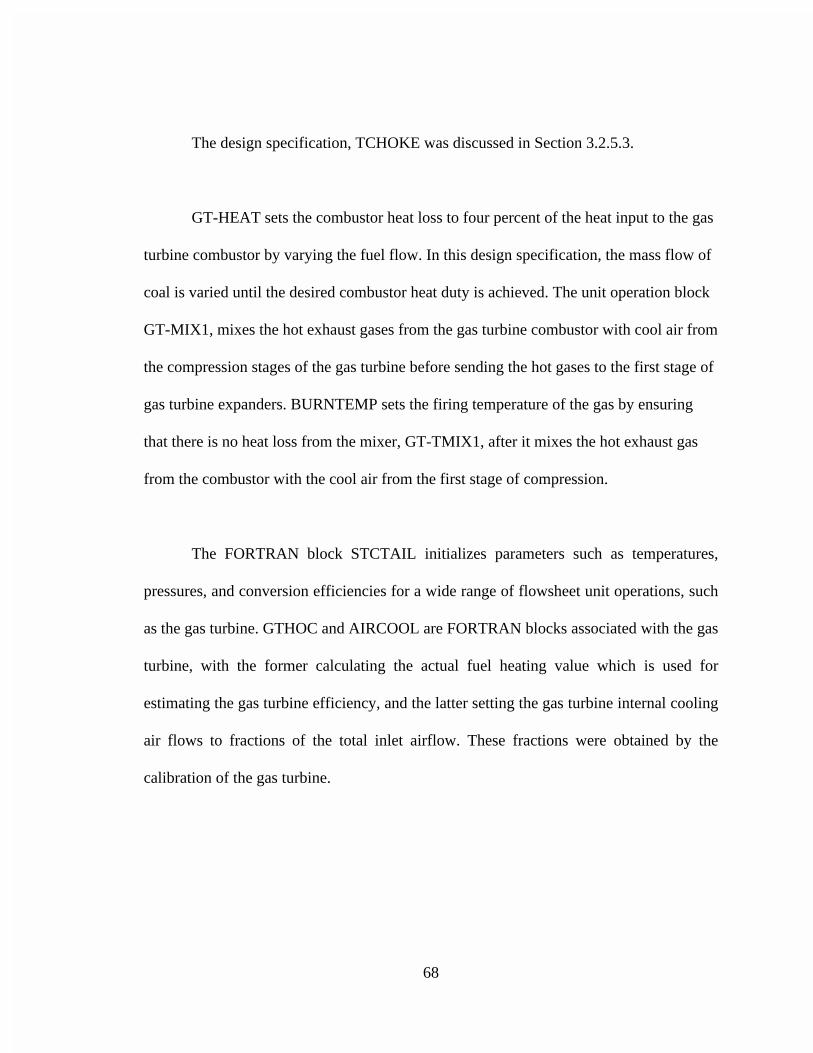
68
The design specification, TCHOKE was discussed in Section 3.2.5.3.
GT-HEAT sets the combustor heat loss to four percent of the heat input to the gas
turbine combustor by varying the fuel flow. In this design specification, the mass flow of
coal is varied until the desired combustor heat duty is achieved. The unit operation block
GT-MIX1, mixes the hot exhaust gases from the gas turbine combustor with cool air from
the compression stages of the gas turbine before sending the hot gases to the first stage of
gas turbine expanders. BURNTEMP sets the firing temperature of the gas by ensuring
that there is no heat loss from the mixer, GT-TMIX1, after it mixes the hot exhaust gas
from the combustor with the cool air from the first stage of compression.
The FORTRAN block STCTAIL initializes parameters such as temperatures,
pressures, and conversion efficiencies for a wide range of flowsheet unit operations, such
as the gas turbine. GTHOC and AIRCOOL are FORTRAN blocks associated with the gas
turbine, with the former calculating the actual fuel heating value which is used for
estimating the gas turbine efficiency, and the latter setting the gas turbine internal cooling
air flows to fractions of the total inlet airflow. These fractions were obtained by the
calibration of the gas turbine.
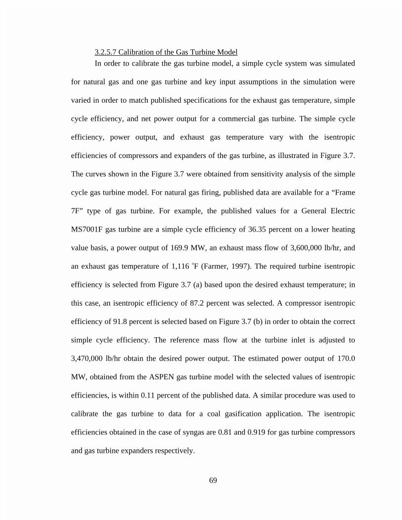
69
3.2.5.7 Calibration of the Gas Turbine Model
In order to calibrate the gas turbine model, a simple cycle system was simulated
for natural gas and one gas turbine and key input assumptions in the simulation were
varied in order to match published specifications for the exhaust gas temperature, simple
cycle efficiency, and net power output for a commercial gas turbine. The simple cycle
efficiency, power output, and exhaust gas temperature vary with the isentropic
efficiencies of compressors and expanders of the gas turbine, as illustrated in Figure 3.7.
The curves shown in the Figure 3.7 were obtained from sensitivity analysis of the simple
cycle gas turbine model. For natural gas firing, published data are available for a “Frame
7F” type of gas turbine. For example, the published values for a General Electric
MS7001F gas turbine are a simple cycle efficiency of 36.35 percent on a lower heating
value basis, a power output of 169.9 MW, an exhaust mass flow of 3,600,000 lb/hr, and
an exhaust gas temperature of 1,116 oF (Farmer, 1997). The required turbine isentropic
efficiency is selected from Figure 3.7 (a) based upon the desired exhaust temperature; in
this case, an isentropic efficiency of 87.2 percent was selected. A compressor isentropic
efficiency of 91.8 percent is selected based on Figure 3.7 (b) in order to obtain the correct
simple cycle efficiency. The reference mass flow at the turbine inlet is adjusted to
3,470,000 lb/hr obtain the desired power output. The estimated power output of 170.0
MW, obtained from the ASPEN gas turbine model with the selected values of isentropic
efficiencies, is within 0.11 percent of the published data. A similar procedure was used to
calibrate the gas turbine to data for a coal gasification application. The isentropic
efficiencies obtained in the case of syngas are 0.81 and 0.919 for gas turbine compressors
and gas turbine expanders respectively.

70
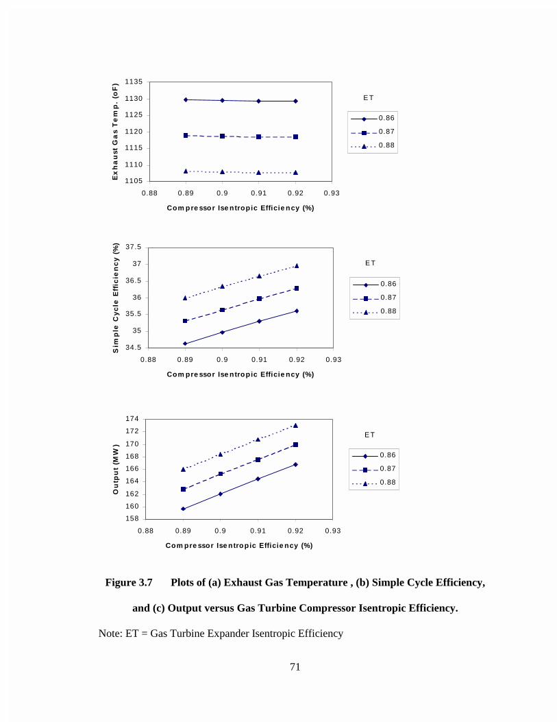
71
1105
1110
1115
1120
1125
1130
1135
0.88 0.89 0.9 0.91 0.92 0.93
Com pre ssor Ise ntropic Efficie ncy (%)
Ex
ha
ust
Ga
s T
em
p.
(oF
)0.86
0.87
0.88
E T
34.5
35
35.5
36
36.5
37
37.5
0.88 0.89 0.9 0.91 0.92 0.93
Com pre ssor Ise ntropic Efficie ncy (%)
Sim
ple
Cy
cle
Eff
icie
nc
y (
%)
0.86
0.87
0.88
E T
158
160
162
164
166
168
170
172
174
0.88 0.89 0.9 0.91 0.92 0.93
Com pre ssor Ise ntropic Efficie ncy (%)
Ou
tpu
t (M
W)
0.86
0.87
0.88
E T
Figure 3.7 Plots of (a) Exhaust Gas Temperature , (b) Simple Cycle Efficiency,
and (c) Output versus Gas Turbine Compressor Isentropic Efficiency.
Note: ET = Gas Turbine Expander Isentropic Efficiency
72
3.2.6 Steam CycleThe steam cycle section of the IGCC consists of the heat recovery steam
generator, auxiliaries and steam turbine. The steam cycle is shown in Table 3.6 and
Figure 3.8.
3.2.6.1 Heat Recovery Steam Generation (HRSG)
The operations of the HRSG are to preheat boiler feed water, reheat intermediate
pressure steam, supplement high pressure and 100 psia steam generation, and to superheat
high pressure steam. The HRSG is arranged in the following order and shown in detail in
Table 3.7 and Figure 3.9.
1. Superheater and reheater in parallel,
2. High pressure evaporator,
3. Economizer,
4. 100 psia boiler, and
5. Economizer.
The HRSG consists of a superheater at a pressure of 1465 psia and a temperature
of 997 oF, a reheater at 997 oF, two economizers, a high pressure boiler, and a low
pressure boiler. The inlet steam to the high pressure economizer and the makeup water for
steam generation is initialized in the ASPEN input file through FORTRAN block
SETSTEAM. The low pressure boiler is used to produce steam for the deaerator for the
flue gas leaving the economizer at 366 oF. The heat losses in the HRSG process are
accounted for through block QSPLIT shown in Table 3.6 and Figure 3.8
73
The hot exhaust gases from the gas turbine section, represented by GTPOC, are
cooled by a series of heat exchangers, modeled by blocks SH-HRSG, HP-HRSG, E2-
HRSG, LP-HRSG, and E1-HRSG in that order and are illustrated in Figure 3.4. The heat
streams obtained from three of the blocks, namely E1-HRSG, E2-HRSG, and HP-HRSG
are mixed in a mixer, simulated by QMIX. The heat stream from SH-HRSG, QSH-HRSG
is split into three heat streams by the block QSPLIT. One heat stream is discarded as heat
lost, one of the heat streams, QREHEAT is diverted to block TURBHEAT in steam
turbine section shown in Figure 3.11, and the remaining heat stream, QSUPER, is sent to
the block QMIX.
The total heat from the QMIX block, QTOTHRSG, is sent to the block
ECONOMZR which simulates a heat exchanger. ECONOMZR heats a stream of water to
a temperature of 553 oF. The mass flow of the stream of water, TOECON is calculated by
the FORTRAN block SETSTEAM. The remaining amount of heat available is sent to
block HPBOILER which simulates a high pressure steam boiler in HRSG. The steam
generated by HPBOILER enters the superheater, SUPERHTR and generates superheated
steam at a temperature of 997 oF. which is sent to a high pressure (350 psia) steam
turbine, simulated by block TURB350 as shown in Figure 3.11.
The low pressure (1 psia) steam generated by the block TURB1, representing a
steam turbine, is cooled by a heater simulated by block CONDENSR, as shown in Figure
74
3.8. The condensate from CONDENSR is pumped to 25 psia and delivered as WATER25
to a deaerator, simulated by the block DEAERATOR. DEAERATOR mixes the various
condensates from the auxiliaries section, stream WATER25 and makeup water, which is
required to makeup for the water sent to the fuel saturation unit from the steam cycle
section. The mixed condensate, represented by DEAERH2O is sent to a block H2OSPLIT
which simulates the splitting of the total condensate to streams TOECON, TOB100,
TO565PSI, and TO65PSI. The ratios of the split are calculated by the FORTRAN block
SETSTEAM.
Streams TOECON and TOB100 are sent to the blocks ECONMZR and BOIL100,
respectively, in the HRSG section. BOIL100 simulates the generation of 100 psia steam.
The steam from BOIL100 is split by the block SPLIT100 into streams SLXSTM and
STM100, both of which are sent to the auxiliaries section shown in Figure 3.10. The unit
operation blocks of the auxiliaries section are listed in Table 3.8.
The water streams TO565PSI and TO65PSI from the block H2OSPLIT are also
sent to the auxiliaries section. The block CLAUS565 in the auxiliaries section heats the
stream TO565PSI and generates steam of 565 psia pressure which is sent to the block
TURBREHT and is further heated by the heat stream QREHEAT to a temperature of 996
oF.
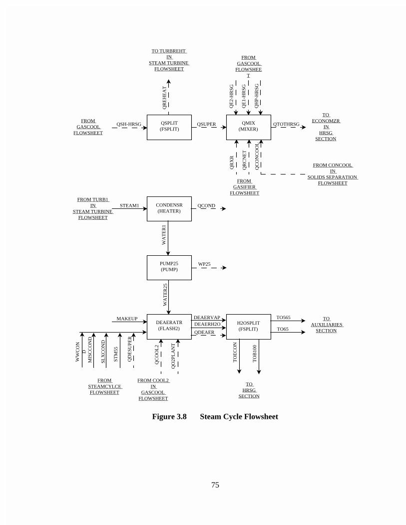
75
QSPLIT (FSPLIT)
QMIX (MIXER)
CONDENSR (HEATER)
PUMP25 (PUMP)
DEAERATR (FLASH2)
H2OSPLIT (FSPLIT)
FROM GASCOOL
FLOWSHEET
FROM GASIFIER
FLOWSHEET
TO ECONOMZR
IN HRSG
SECTION
FROM CONCOOL IN
SOLIDS SEPARATION FLOWSHEET
TO AUXILIARIES
SECTION
TO HRSG
SECTION
FROM COOL2 IN
GASCOOL FLOWSHEET
FROM STEAMCYLCE FLOWSHEET
FROM TURB1 IN
STEAM TURBINE FLOWSHEET
FROM GASCOOL
FLOWSHEET
QSH-HRSG QSUPER QTOTHRSG
QR
EH
EA
T
QR
XR
QR
CN
ET
QC
ON
CO
OL
QE
2-H
RSG
QE
1-H
RSG
QH
P-H
RSG
STEAM1
WA
TE
R1
QCOND
WP25
WA
TE
R25
MAKEUP DEAERVAPDEAERH2O
QDEAER
TO565
TO65
TO
EC
ON
TO
B10
0
QO
2PL
AN
T
QC
OO
L2
WW
CO
ND
MIS
CC
ON
D
SLX
CO
ND
STM
55
QD
ESU
PER
TO TURBREHT IN
STEAM TURBINE FLOWSHEET
Figure 3.8 Steam Cycle Flowsheet
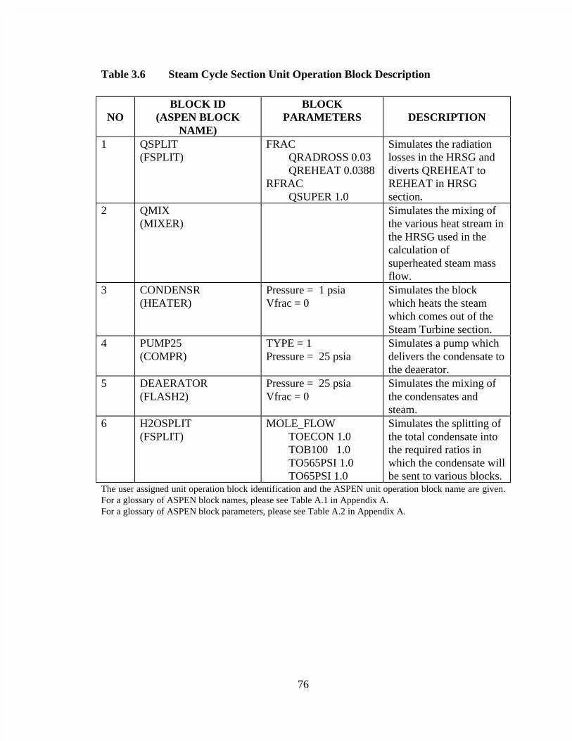
76
Table 3.6 Steam Cycle Section Unit Operation Block Description
NOBLOCK ID
(ASPEN BLOCKNAME)
BLOCKPARAMETERS DESCRIPTION
1 QSPLIT(FSPLIT)
FRAC QRADROSS 0.03 QREHEAT 0.0388RFRAC QSUPER 1.0
Simulates the radiationlosses in the HRSG anddiverts QREHEAT toREHEAT in HRSGsection.
2 QMIX(MIXER)
Simulates the mixing ofthe various heat stream inthe HRSG used in thecalculation ofsuperheated steam massflow.
3 CONDENSR(HEATER)
Pressure = 1 psiaVfrac = 0
Simulates the blockwhich heats the steamwhich comes out of theSteam Turbine section.
4 PUMP25(COMPR)
TYPE = 1Pressure = 25 psia
Simulates a pump whichdelivers the condensate tothe deaerator.
5 DEAERATOR(FLASH2)
Pressure = 25 psiaVfrac = 0
Simulates the mixing ofthe condensates andsteam.
6 H2OSPLIT(FSPLIT)
MOLE_FLOW TOECON 1.0 TOB100 1.0 TO565PSI 1.0 TO65PSI 1.0
Simulates the splitting ofthe total condensate intothe required ratios inwhich the condensate willbe sent to various blocks.
The user assigned unit operation block identification and the ASPEN unit operation block name are given.For a glossary of ASPEN block names, please see Table A.1 in Appendix A.For a glossary of ASPEN block parameters, please see Table A.2 in Appendix A.
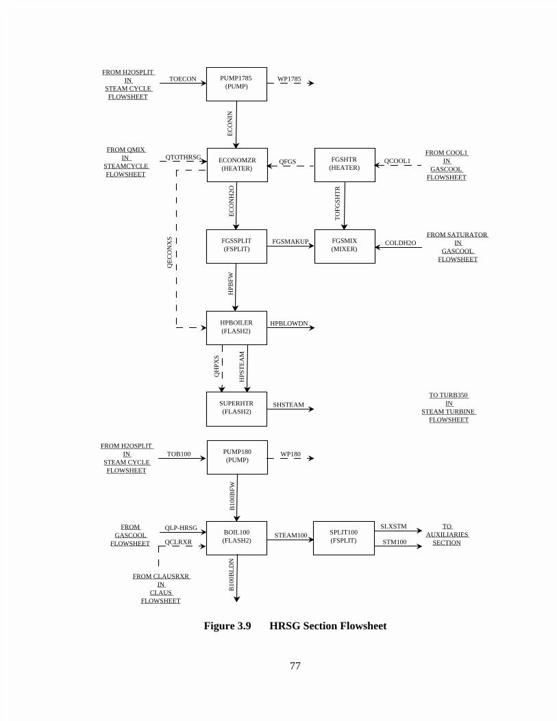
77
PUMP1785 (PUMP)
ECONOMZR (HEATER)
FGSMIX (MIXER)
HPBOILER (FLASH2)
SUPERHTR (FLASH2)
PUMP180 (PUMP)
BOIL100 (FLASH2)
SPLIT100 (FSPLIT)
FGSSPLIT (FSPLIT)
FGSHTR (HEATER)
FROM COOL1 IN
GASCOOL FLOWSHEET
FROM SATURATOR IN
GASCOOL FLOWSHEET
TO TURB350 IN
STEAM TURBINE FLOWSHEET
TO AUXILIARIES
SECTION
FROM GASCOOL
FLOWSHEET
FROM CLAUSRXR IN
CLAUS FLOWSHEET
FROM H2OSPLIT IN
STEAM CYCLE FLOWSHEET
FROM QMIX IN
STEAMCYCLE FLOWSHEET
TOECON
EC
ON
IN
QTOTHRSG
EC
ON
H2O
HP
BF
W
QE
CO
NX
S
HPBLOWDN
QCOOL1
COLDH2O
TO
FGSH
TR
QH
PXS
HPS
TE
AM
SHSTEAM
TOB100 WP180
B10
0BF
WB
100B
LD
N
QLP-HRSG
QCLRXRSTEAM100
SLXSTM
STM100
WP1785
QFGS
FGSMAKUP
FROM H2OSPLIT IN
STEAM CYCLE FLOWSHEET
Figure 3.9 HRSG Section Flowsheet
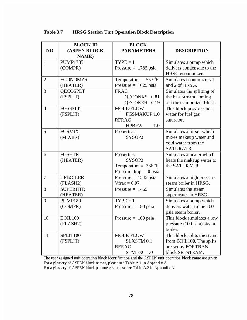
78
Table 3.7 HRSG Section Unit Operation Block Description
NOBLOCK ID
(ASPEN BLOCKNAME)
BLOCKPARAMETERS DESCRIPTION
1 PUMP1785(COMPR)
TYPE = 1Pressure = 1785 psia
Simulates a pump whichdelivers condensate to theHRSG economizer.
2 ECONOMZR(HEATER)
Temperature = 553 oFPressure = 1625 psia
Simulates economizers 1and 2 of HRSG.
3 QECOSPLT(FSPLIT)
FRAC QECONXS 0.81 QECOREH 0.19
Simulates the splitting ofthe heat stream comingout the economizer block.
4 FGSSPLIT(FSPLIT)
MOLE-FLOW FGSMAKUP 1.0RFRAC HPBFW 1.0
This block provides hotwater for fuel gassaturator.
5 FGSMIX(MIXER)
Properties SYSOP3
Simulates a mixer whichmixes makeup water andcold water from theSATURATR.
6 FGSHTR(HEATER)
Properties SYSOP3Temperature = 366 oFPressure drop = 0 psia
Simulates a heater whichheats the makeup water tothe SATURATR.
7 HPBOILER(FLASH2)
Pressure = 1545 psiaVfrac = 0.97
Simulates a high pressuresteam boiler in HRSG.
8 SUPERHTR(HEATER)
Pressure = 1465 Simulates the steamsuperheater in HRSG.
9 PUMP180(COMPR)
TYPE = 1Pressure = 180 psia
Simulates a pump whichdelivers water to the 100psia steam boiler.
10 BOIL100(FLASH2)
Pressure = 100 psia This block simulates a lowpressure (100 psia) steamboiler.
11 SPLIT100(FSPLIT)
MOLE-FLOW SLXSTM 0.1RFRAC STM100 1.0
This block splits the steamfrom BOIL100. The splitsare set by FORTRANblock SETSTEAM.
The user assigned unit operation block identification and the ASPEN unit operation block name are given.For a glossary of ASPEN block names, please see Table A.1 in Appendix A.For a glossary of ASPEN block parameters, please see Table A.2 in Appendix A.
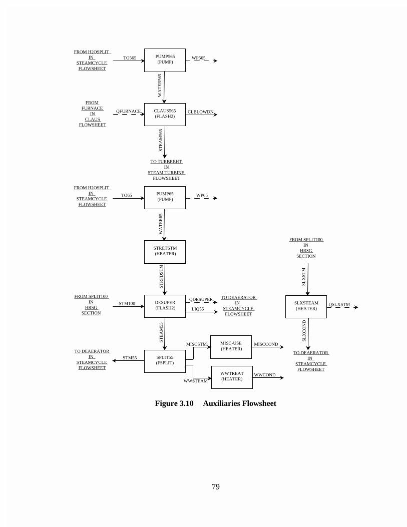
79
PUMP65 (PUMP)
PUMP565 (PUMP)
CLAUS565 (FLASH2)
STRETSTM (HEATER)
DESUPER (FLASH2)
SPLIT55 (FSPLIT)
MISC-USE (HEATER)
WWTREAT (HEATER)
SLXSTEAM (HEATER)
TO565
TO65 WP65
ST
EA
M56
5W
AT
ER
65S
TR
FD
ST
M
STM100LIQ55
ST
EA
M55
STM55
MISCSTM
WWSTEAM
MISCCOND
WWCOND
SL
XS
TM
SLX
CO
ND
QSLXSTM
WA
TE
R56
5
FROM SPLIT100 IN
HRSG SECTION
TO DEAERATOR IN
STEAMCYCLE FLOWSHEET
TO DEAERATOR IN
STEAMCYCLE FLOWSHEET
TO DEAERATOR IN
STEAMCYCLE FLOWSHEET
FROM SPLIT100 IN
HRSG SECTION
FROM H2OSPLIT IN
STEAMCYCLE FLOWSHEET
FROM H2OSPLIT IN
STEAMCYCLE FLOWSHEET
FROM FURNACE
IN CLAUS
FLOWSHEET
WP565
QFURNACE CLBLOWDN
TO TURBREHT IN
STEAM TURBINE FLOWSHEET
QDESUPER
Figure 3.10 Auxiliaries Flowsheet
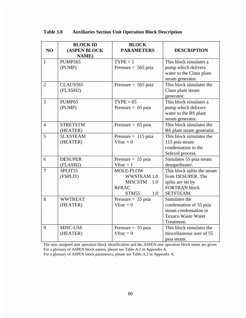
80
Table 3.8 Auxiliaries Section Unit Operation Block Description
NOBLOCK ID
(ASPEN BLOCKNAME)
BLOCKPARAMETERS DESCRIPTION
1 PUMP565(PUMP)
TYPE = 1Pressure = 565 psia
This block simulates apump which deliverswater to the Claus plantsteam generator.
2 CLAUS565(FLASH2)
Pressure = 565 psia This block simulates theClaus plant steamgenerator.
3 PUMP65(PUMP)
TYPE = 65Pressure = 65 psia
This block simulates apump which deliverswater to the BS plantsteam generator.
4 STRETSTM(HEATER)
Pressure = 65 psia This block simulates theBS plant steam generator.
5 SLXSTEAM(HEATER)
Pressure = 115 psiaVfrac = 0
This block simulates the115 psia steamcondensation in theSelexol process.
6 DESUPER(FLASH2)
Pressure = 55 psiaVfrac = 1
Simulates 55 psia steamdesuperheater.
7 SPLIT55(FSPLIT)
MOLE-FLOW WWSTEAM 1.0 MISCSTM 1.0RFRAC STM55 1.0
This block splits the steamfrom DESUPER. Thesplits are set byFORTRAN blockSETSTEAM.
8 WWTREAT(HEATER)
Pressure = 55 psiaVfrac = 0
Simulates thecondensation of 55 psiasteam condensation inTexaco Waste WaterTreatment.
9 MISC-USE(HEATER)
Pressure = 55 psiaVfrac = 0
This block simulates themiscellaneous user of 55psia steam.
The user assigned unit operation block identification and the ASPEN unit operation block name are given.For a glossary of ASPEN block names, please see Table A.1 in Appendix A.For a glossary of ASPEN block parameters, please see Table A.2 in Appendix A.
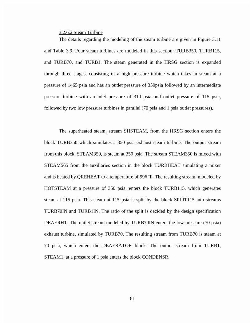
81
3.2.6.2 Steam Turbine
The details regarding the modeling of the steam turbine are given in Figure 3.11
and Table 3.9. Four steam turbines are modeled in this section: TURB350, TURB115,
and TURB70, and TURB1. The steam generated in the HRSG section is expanded
through three stages, consisting of a high pressure turbine which takes in steam at a
pressure of 1465 psia and has an outlet pressure of 350psia followed by an intermediate
pressure turbine with an inlet pressure of 310 psia and outlet pressure of 115 psia,
followed by two low pressure turbines in parallel (70 psia and 1 psia outlet pressures).
The superheated steam, stream SHSTEAM, from the HRSG section enters the
block TURB350 which simulates a 350 psia exhaust steam turbine. The output stream
from this block, STEAM350, is steam at 350 psia. The stream STEAM350 is mixed with
STEAM565 from the auxiliaries section in the block TURBHEAT simulating a mixer
and is heated by QREHEAT to a temperature of 996 oF. The resulting stream, modeled by
HOTSTEAM at a pressure of 350 psia, enters the block TURB115, which generates
steam at 115 psia. This steam at 115 psia is split by the block SPLIT115 into streams
TURB70IN and TURB1IN. The ratio of the split is decided by the design specification
DEAERHT. The outlet stream modeled by TURB70IN enters the low pressure (70 psia)
exhaust turbine, simulated by TURB70. The resulting stream from TURB70 is steam at
70 psia, which enters the DEAERATOR block. The output stream from TURB1,
STEAM1, at a pressure of 1 psia enters the block CONDENSR.
82
3.2.6.3 Design Specifications and FORTRAN blocks
The design specifications used in the steam cycle section of the model are
DEAERTHT and STMTEMP.
DEAERHT is used to operate the deaerator approximately adiabatically. The heat
stream leaving the block DEAERHT is should be less than 100.0 BTU/hr. This design
specification is achieved by varying the ratio of splitting of the stream, SPLIT115.
STMTEMP sets the temperature of the stream leaving the HRSG reheat block to be
equal to that of the stream leaving superheater. This is achieved by varying the split ratio
of the heat stream, QSH-HRSG, which splits into heat streams QSUPER and QREHEAT.
QSH-HRSG is obtained by cooling the products of combustion from the gas turbine,
GTPOC in the block QSPLIT.
FORTRAN block SETMAKEUP sets the steam cycle makeup water and the
FORTRAN block SETSTEAM calculates the various mass flows of water streams such
as those represented by TOECON, TOB100, TO565PSI, and TO65PSI. The required
water circulation rate to the heat economizers in HRSG is calculated by FORTRAN block
SETSTEAM, based on the temperature of the superheated steam, 997 oF and the
temperature at which the water enters the HRSG from the deaerator, 244 oF. The flow
rates of water and steam to other parts of the model is also calculated by the same block.
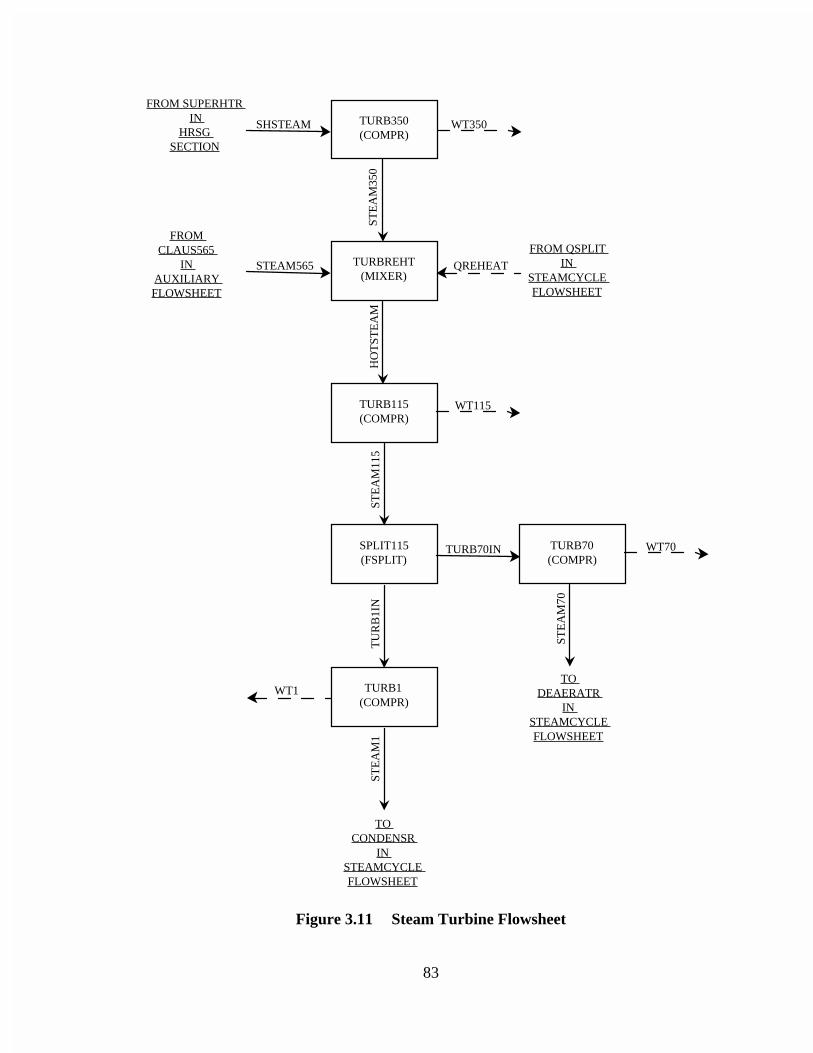
83
TURB350 (COMPR)
TURBREHT (MIXER)
TURB115 (COMPR)
TURB1 (COMPR)
TURB70 (COMPR)
SPLIT115 (FSPLIT)
FROM SUPERHTR IN
HRSG SECTION
FROM CLAUS565
IN AUXILIARY FLOWSHEET
FROM QSPLIT IN
STEAMCYCLE FLOWSHEET
TO DEAERATR
IN STEAMCYCLE FLOWSHEET
TO CONDENSR
IN STEAMCYCLE FLOWSHEET
SHSTEAM WT350
STEAM565
STE
AM
115
WT70ST
EA
M70
STE
AM
1
WT1
WT115
TURB70IN
TU
RB
1IN
HO
TST
EA
M
QREHEAT
STE
AM
350
Figure 3.11 Steam Turbine Flowsheet
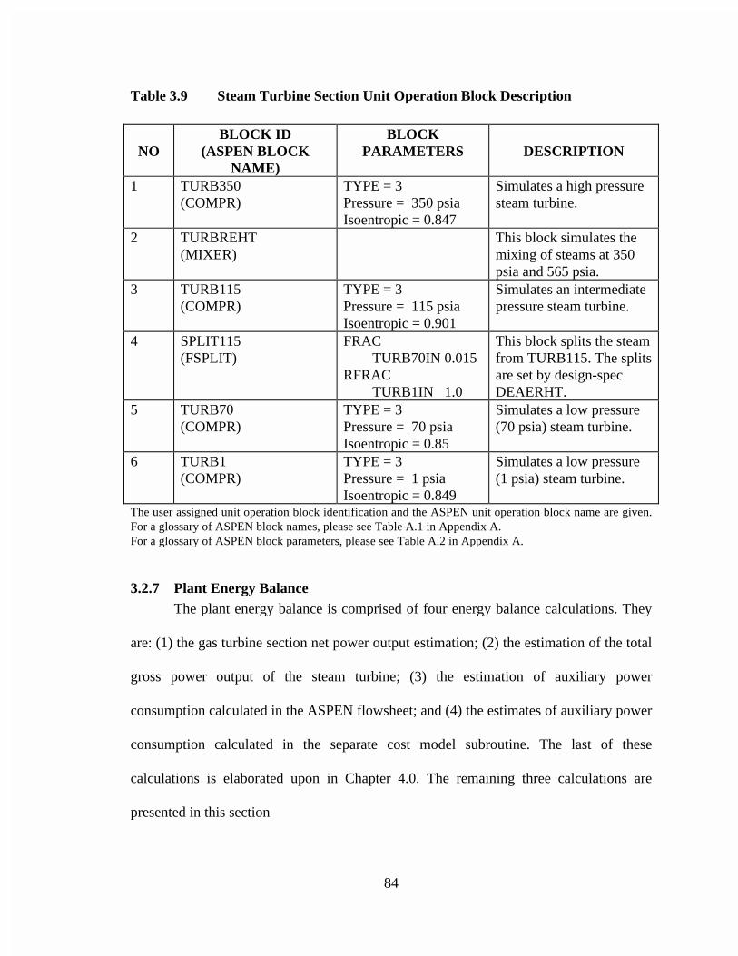
84
Table 3.9 Steam Turbine Section Unit Operation Block Description
NOBLOCK ID
(ASPEN BLOCKNAME)
BLOCKPARAMETERS DESCRIPTION
1 TURB350(COMPR)
TYPE = 3Pressure = 350 psiaIsoentropic = 0.847
Simulates a high pressuresteam turbine.
2 TURBREHT(MIXER)
This block simulates themixing of steams at 350psia and 565 psia.
3 TURB115(COMPR)
TYPE = 3Pressure = 115 psiaIsoentropic = 0.901
Simulates an intermediatepressure steam turbine.
4 SPLIT115(FSPLIT)
FRAC TURB70IN 0.015RFRAC TURB1IN 1.0
This block splits the steamfrom TURB115. The splitsare set by design-specDEAERHT.
5 TURB70(COMPR)
TYPE = 3Pressure = 70 psiaIsoentropic = 0.85
Simulates a low pressure(70 psia) steam turbine.
6 TURB1(COMPR)
TYPE = 3Pressure = 1 psiaIsoentropic = 0.849
Simulates a low pressure(1 psia) steam turbine.
The user assigned unit operation block identification and the ASPEN unit operation block name are given.For a glossary of ASPEN block names, please see Table A.1 in Appendix A.For a glossary of ASPEN block parameters, please see Table A.2 in Appendix A.
3.2.7 Plant Energy BalanceThe plant energy balance is comprised of four energy balance calculations. They
are: (1) the gas turbine section net power output estimation; (2) the estimation of the total
gross power output of the steam turbine; (3) the estimation of auxiliary power
consumption calculated in the ASPEN flowsheet; and (4) the estimates of auxiliary power
consumption calculated in the separate cost model subroutine. The last of these
calculations is elaborated upon in Chapter 4.0. The remaining three calculations are
presented in this section
85
Assuming a generator loss of 0.5 percent, the net gas turbine power output is
calculated to be the sum of the work done by the gas turbine expanders and work required
by the gas turbine compressors.
The total gross output of the steam turbine is the sum of the total work done by
the four steam turbines.
The auxiliary power consumption is estimated in three different sections of the
performance model: (1) the power consumed by the compressors in the Claus plant and
Beavon-Stretford plant; (2) the power consumption by all the pumps in the model
delivering slurry or water; and (3) the power consumption by the oxygen plant assuming
that 1 lbmol/hr of 95 percent purity oxygen requires 6000 watts of power. The auxiliary
power consumption models are developed and included in the cost model of the IGCC
system. These include models for auxiliary power consumption of coal handling, oxidant
feed, gasification, low temperature gas cooling, acid gas removal, Claus and Beavon-
Stretford plants, gas turbine, process condensate, boiler feed water, steam cycle, and
general facilities sections.
86
3.3 Convergence Sequence
The convergence sequence for the model simulation is based on nine design
specifications and seven FORTRAN blocks. Most of the design specifications and
FORTRAN blocks have been described in earlier sections of this chapter and the rest are
elaborated upon in this Section.
The FORTRAN block SETFEED maintains the water-to-coal ratio in the model
by setting the mass flow of water to the gasifier based upon calculation that the coal
slurry has 66.5 percent of solids by weight.
The Oxygen/Coal ratio is varied by a design specification, SETOXYG, in order to
achieve the specified syngas exit temperature and overcome a two percent heat loss from
the gasifier. The design specifications SETCLAIR and SETBSAIR set the air flow rates
to the Claus unit and the Beavon-Stretford tail gas treatment units, respectively.
SETCLAIR is designed such that the air provided to the Claus plant is enough to convert
one-third of the hydrogen sulfide to elemental sulfur. SETBSAIR provides one percent
excess oxygen to completely oxidize the constituents of the tail gas sent to the Beavon-
Stretford plant.
The convergence sequence starts with the initialization of key input variables in
the FORTRAN block STCTAIL. Then the gasification, high temperature gas cooling, and
87
solid separation process area sequences are called by the master sequence. This is
followed by the low temperature gas cooling sequence. The Selexol process and the fuel
gas saturation process area sequences are specified next. Then the gas turbine flowsheet
sequence is specified followed by the Claus plant and the Beavon-Stretford plant
sequences. Then the gas side of the HRSG, and the entire steam cycle sequences are
specified. Finally, the FORTAN block which presents user defined results, SUMMARY
is attached to the sequence followed by the cost model FORTRAN subroutine,
TEXCOST.
3.4 Environmental Emissions
SO2 emissions from IGCC systems are controlled by removing sulfur species from
the syngas prior to combustion in the gas turbine. NOx emissions tend to be low for this
particular IGCC system for two reasons. The first is that there is very little fuel-bound
nitrogen in the fuel gas. The second reason is that thermal NO formation is low because
of the low syngas heating value and correspondingly relatively low adiabatic flame
temperature. A primary purpose of the gas cleanup system is to protect the gas turbine
from contaminants in the fuel. Hence, no post-combustion control is assumed. However,
it is possible to further control NOx emissions, for example, through use of Selective
Catalytic Reduction (SCR) downstream of the gas turbine. The emission rates of these
pollutants are lower than for conventional power plants and for many advanced coal-
based power generation alternatives. CO2 emissions are lower than for conventional coal-
88
fired power plants because of the higher thermal efficiency of the IGCC system (e.g.,
nearly 40 percent in this case versus typical values of 35 percent for conventional
pulverized coal-fired power plants).
3.4.1 NOx EmissionsThe generation of NO and NO2 from the gas turbine has been modeled in the
present study. Both the fuel NOx as well as thermal NOx have been taken into
consideration for the estimation of NO and NO2. The default assumptions made for these
estimations are that fuel NO is 95 percent by volume of the fuel NOx, and that the fraction
of ammonia that is converted to fuel NOx is 0.90. The conversion rate of nitrogen to NOX
during the gas turbine combustion is assumed to be 0.00045. Atmospheric emission rates
are calculated on a lb/MMBTU basis as part of the model output.
3.4.2 Particulate Matter EstimationsPM emissions are controlled in the syngas cleanup system prior to the gas turbine
and therefore, particulate matter emissions from the gas turbine are not modeled in the
present model.
3.4.3 CO and CO2 EmissionsCO emissions from the power plant are assumed to come from the gas turbine
section of the plant. The fraction of CO that is converted to CO2 in the gas turbine is
assumed to be 0.99985. Aside from the gas turbine, CO2 is also emitted by the Beavon-
Stretford tail gas treatment unit. The emissions are expressed in terms of lb/kWh.
89
3.4.4 SO2 EmissionsSO2 emissions from the IGCC system are assumed to the result from combustion
of syngas in the gas turbine. The SO2 emissions from the gas turbine are due to oxidation
of H2S and COS in the fuel gas. The amount of H2S and COS in the fuel gas can be varied
by changing the removal efficiency of the Selexol process. The emissions are calculated
on a lb/MMBTU basis.
90
4.0 DOCUMENTATION OF THE AUXILIARY POWER MODEL FOR THECOAL-FUELED TEXACO GASIFIER-BASED IGCC SYSTEM WITHRADIANT AND CONVECTIVE HIGH TEMPERATURE GAS COOLING
Significant amounts of electrical power are consumed by certain process areas of
the power plant for the operation of components such as pumps and conveyors. These
auxiliary power requirements reduce the net power output of the plant. The auxiliary
power requirements are functions of the process variables of the system. Only a few of
the auxiliary loads are modeled directly in the ASPEN performance model. They are the
total power consumption by the compressors and the centrifugal pumps in the system. All
other auxiliary loads are modeled in the cost model subroutine linked to the performance
model. These auxiliary power models are described in this chapter.
4.1 Coal Handling
The Texaco IGCC system uses a coal slurry with typically 66.5 weight percent of
solids as feed to the gasifier. Coal handling involves coal unloading, stacking,
reclamation, and conveying equipment followed by three operating and one spare train of
wet grinding equipment. To estimate the auxiliary power requirements of the coal
handling unit, a predictive model was developed by Rocha and Frey (1997) using 13 data
points obtained from the sources listed in Table 4.1. The coal feed rate was chosen as the
independent variable for development of an auxiliary power model. Two models were
selected for consideration: power consumed per slurry train vs. coal feed rate per slurry
91
train; and total power consumed by the slurry preparation process area vs. total coal flow
to slurry preparation. The power consumed per slurry train vs. coal feed rate per slurry
train produced a standard error of 1,183 kW per train and a R2 of 0.716, whereas the
standard error for the other model is 2,949 kW for the entire plant and the R2 value is
0.807. Because of the higher R2 value, the latter model was selected.
We, CH = 1.04 mcf, Ch,i (4-1)
where,
We, CH = Auxiliary power consumption of the coal handling process, kW.
mcf, CH, i = Coal feed rate, tons/day.
3,300 ≤ mcf, CH, i ≤ 20,000 tons per day as-received.
The model and data are shown in Figure 4.1. The model fit is greatly influenced
by the data point that is at 20,000 tons/day gasifier coal feed rate (McNamee and White,
1986). A much better fit could occur if this value was removed from the power
consumption model consideration. The data point was not removed because no reason
could be found to exclude the value from the development of the power consumption
model.
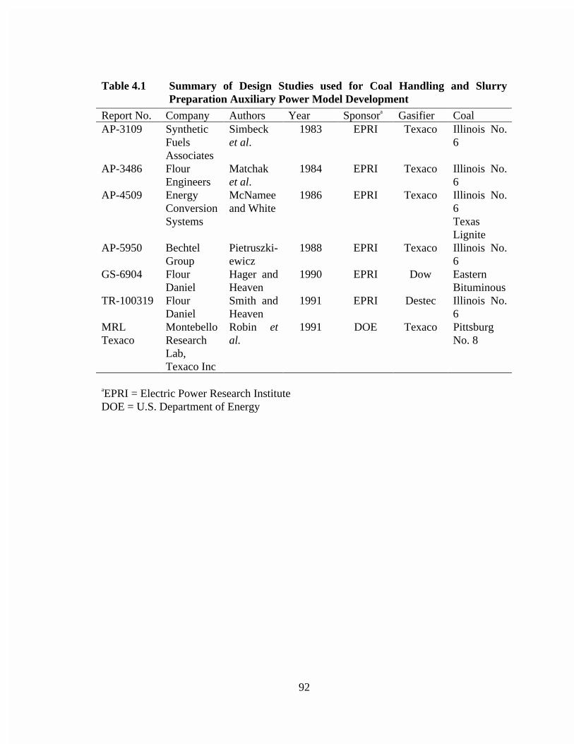
92
Table 4.1 Summary of Design Studies used for Coal Handling and SlurryPreparation Auxiliary Power Model Development
Report No. Company Authors Year Sponsora Gasifier CoalAP-3109 Synthetic
FuelsAssociates
Simbecket al.
1983 EPRI Texaco Illinois No.6
AP-3486 FlourEngineers
Matchaket al.
1984 EPRI Texaco Illinois No.6
AP-4509 EnergyConversionSystems
McNameeand White
1986 EPRI Texaco Illinois No.6TexasLignite
AP-5950 BechtelGroup
Pietruszki-ewicz
1988 EPRI Texaco Illinois No.6
GS-6904 FlourDaniel
Hager andHeaven
1990 EPRI Dow EasternBituminous
TR-100319 FlourDaniel
Smith andHeaven
1991 EPRI Destec Illinois No.6
MRLTexaco
MontebelloResearchLab,Texaco Inc
Robin etal.
1991 DOE Texaco PittsburgNo. 8
aEPRI = Electric Power Research InstituteDOE = U.S. Department of Energy
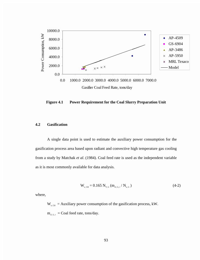
93
0.0
2000.0
4000.0
6000.0
8000.0
10000.0
0.0 1000.0 2000.0 3000.0 4000.0 5000.0 6000.0 7000.0
Gasifier Coal Feed Rate, tons/day
Pow
er C
onsu
mpt
ion,
kW AP-4509
GS-6904
AP-3486
AP-5950
MRL Texaco
Model
Figure 4.1 Power Requirement for the Coal Slurry Preparation Unit
4.2 Gasification
A single data point is used to estimate the auxiliary power consumption for the
gasification process area based upon radiant and convective high temperature gas cooling
from a study by Matchak et al. (1984). Coal feed rate is used as the independent variable
as it is most commonly available for data analysis.
We, CH = 0.165 NT, G (mcf, G, i / No, G ) (4-2)
where,
We, CH = Auxiliary power consumption of the gasification process, kW.
mcf, G, i = Coal feed rate, tons/day.
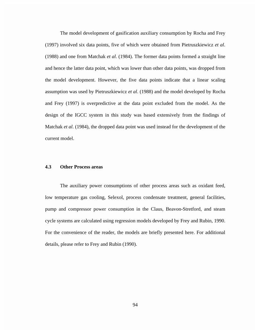
94
The model development of gasification auxiliary consumption by Rocha and Frey
(1997) involved six data points, five of which were obtained from Pietruszkiewicz et al.
(1988) and one from Matchak et al. (1984). The former data points formed a straight line
and hence the latter data point, which was lower than other data points, was dropped from
the model development. However, the five data points indicate that a linear scaling
assumption was used by Pietruszkiewicz et al. (1988) and the model developed by Rocha
and Frey (1997) is overpredictive at the data point excluded from the model. As the
design of the IGCC system in this study was based extensively from the findings of
Matchak et al. (1984), the dropped data point was used instead for the development of the
current model.
4.3 Other Process areas
The auxiliary power consumptions of other process areas such as oxidant feed,
low temperature gas cooling, Selexol, process condensate treatment, general facilities,
pump and compressor power consumption in the Claus, Beavon-Stretford, and steam
cycle systems are calculated using regression models developed by Frey and Rubin, 1990.
For the convenience of the reader, the models are briefly presented here. For additional
details, please refer to Frey and Rubin (1990).
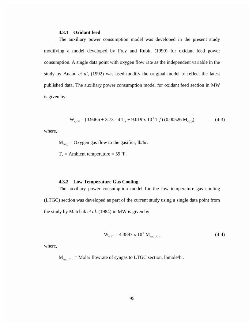
95
4.3.1 Oxidant feedThe auxiliary power consumption model was developed in the present study
modifying a model developed by Frey and Rubin (1990) for oxidant feed power
consumption. A single data point with oxygen flow rate as the independent variable in the
study by Anand et al, (1992) was used modify the original model to reflect the latest
published data. The auxiliary power consumption model for oxidant feed section in MW
is given by:
We, OF = (0.9466 + 3.73 - 4 TA + 9.019 x 10⁻⁶ TA
2) (0.00526 MO,G,i) (4-3)
where,
MO,G,i = Oxygen gas flow to the gasifier, lb/hr.
TA = Ambient temperature = 59 oF.
4.3.2 Low Temperature Gas CoolingThe auxiliary power consumption model for the low temperature gas cooling
(LTGC) section was developed as part of the current study using a single data point from
the study by Matchak et al. (1984) in MW is given by
We, LT = 4.3887 x 10⁻⁵ Msyn, LT, o (4-4)
where,
Msyn, LT, o = Molar flowrate of syngas to LTGC section, lbmole/hr.
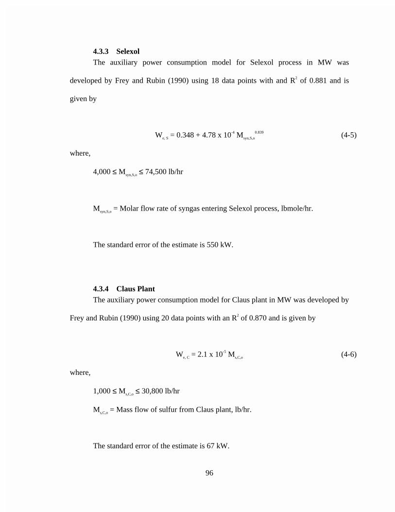
96
4.3.3 SelexolThe auxiliary power consumption model for Selexol process in MW was
developed by Frey and Rubin (1990) using 18 data points with and R2 of 0.881 and is
given by
We, S = 0.348 + 4.78 x 10⁻⁴ Msyn,S,o
0.839 (4-5)
where,
4,000 ≤ Msyn,S,o ≤ 74,500 lb/hr
Msyn,S,o = Molar flow rate of syngas entering Selexol process, lbmole/hr.
The standard error of the estimate is 550 kW.
4.3.4 Claus PlantThe auxiliary power consumption model for Claus plant in MW was developed by
Frey and Rubin (1990) using 20 data points with an R2 of 0.870 and is given by
We, C = 2.1 x 10⁻⁵ Ms,C,o (4-6)
where,
1,000 ≤ Ms,C,o ≤ 30,800 lb/hr
Ms,C,o = Mass flow of sulfur from Claus plant, lb/hr.
The standard error of the estimate is 67 kW.
97
4.3.5 Beavon-Stretford UnitThe auxiliary power consumption model for Beavon-Stretford plant in MW was
developed by Frey and Rubin (1990) using 6 data points with an R2 of 1.00 and is given
by
We, BS = 0.0445 + 0.00112 Ms,BS,o (4-7)
where,
9,000 ≤ Ms,BS,o ≤ 18,000 lb/hr
Ms,BS,o = Mass flow of sulfur from BS plant, lb/hr.
4.3.6 Process Condensate TreatmentThe process condensate treatment plant has the following auxiliary power
consumption model, which is developed for the present Texaco IGCC radiant and
convective gasification system using a single data point from the study Matchak et al.
(1984).
We, PC = 3.397 x 10⁻⁶ Ms,BD (4-8)
where,
Ms,BD = Scrubber blowdown flowrate, lb/hr.
4.3.7 Steam CycleThe boiler feed water (BFW) system supplies the water for steam generation in
the HRSG. BFW consists of raw makeup water and the steam turbine condensate. The
steam cycle auxiliary power load is due to the BFW treatment section and it is given as

98
the sum of all the work done by the pumps dealing with this section. These pumps are
modeled in the ASPEN flowsheet.
WBFW = P1785 + P565 + P180 + P65 + P25 (4-9)
where,
WBFW = Auxiliary power consumption by boiler feedwater section, MW
P1785 = Work done on the centrifugal pump which delivers BFW at 1785 psia, MW
P565 = Work done on the centrifugal pump which delivers BFW at 565 psia, MW
P180 = Work done on the centrifugal pump which delivers BFW at 180 psia, MW
P65 = Work done on the centrifugal pump which delivers BFW at 65 psia, MW
P25 = Work done on the centrifugal pump which delivers BFW at 25 psia, MW
4.3.8 General FacilitiesThe general facilities include power requirements for cooling water systems, plant
and instrument air, fuel system, potable and utility water, nitrogen system, process
condensate and effluent water treating. The general facilities auxiliary power load is
estimated as a fraction of all other auxiliary loads with a typical value of 10 percent.
Based on Frey and Rubin (1990) the auxiliary power load model in MW is given by:
We, GF = 0.1 (We, CH + We, CH + We, OF + We, LT + We, S + We, C + We, BS + We, PC + WBFW) (4-10)
99
The sum of all the above auxiliary power loads gives the total auxiliary power
consumption of the power plant, We, AUX in MW.
We, AUX = We, CH+ We, CH + We, OF + We, LT + We, S + We, C
+ We, BS + We, PC + WBFW + We, GF (4-11)
4.4 Net Power Output and Plant Efficiency
The net plant power output is the total power generated from the gas turbines and
steam turbines less the total auxiliary power consumption. The gas and steam turbines
have been modeled as a series of compressors and turbines in ASPEN using the unit
operation block COMPR. This unit operation block requires outlet pressure and
isoentropic efficiencies as parameters. The power consumed by the compressors and the
power generated by the turbines are calculated by the ASPEN performance model. The
net power output is calculated as part of the cost model which is a part of the FORTRAN
subroutine TEXCOST called by the ASPEN input file. The net power output in MW is
given by
MWnet = MWGT + MWST - We, AUX (4-12)
The net plant efficiency on a higher heating value basis is given by
100
HHVxi,CH,cfMnetMW610x414.3=η (4-13)
where,
η = net plant efficiency.
Mcf, CH, i = Coal feed rate, lb/hr.
HHV = Higher heating value of fuel, BTU/lb.
101
5.0 CAPITAL, ANNUAL, AND LEVELIZED COST MODELS OF THECOAL-FUELED TEXACO GASIFIER-BASED IGCC SYSTEM WITHRADIANT AND CONVECTIVE HIGH TEMPERATURE GAS COOLING
This chapter documents the cost model developed for the coal-fueled Texaco
gasifier-based IGCC plant with radiant and convective high temperature gas cooling. The
direct capital costs for all the important process areas of oxidant feed section, coal
handling and slurry preparation, gasification section, low temperature gas cooling section,
Selexol section, Claus sulfur recovery section, Beavon-Stretford tail gas removal section,
boiler feedwater system, process condensate system, gas turbine section, heat recovery
steam generator section, steam turbine section, and general facilities are described in that
order. The annual, and levelized costs of the model are elaborated upon later in the
chapter.
5.1 Direct Capital Cost
New direct cost models for the major process areas in the IGCC system are
presented. For the purpose of estimating the direct capital costs of the plant, the IGCC
plant is divided into thirteen process areas as listed in Table 5.1. The direct cost of a
process section can be adjusted for other years than that year for which they were
developed using the appropriate Chemical Engineering Plant Cost Index (PCI) (Chemical
Engineering Magazine, 1984-1999) as shown in Table 5.2. For example, if a direct capital
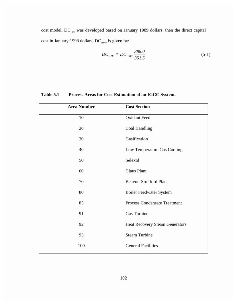
102
cost model, DC1989 was developed based on January 1989 dollars, then the direct capital
cost in January 1998 dollars, DC1998, is given by:
5.351
0.388DCDC 19891998 = (5-1)
Table 5.1 Process Areas for Cost Estimation of an IGCC System.
Area Number Cost Section
10 Oxidant Feed
20 Coal Handling
30 Gasification
40 Low Temperature Gas Cooling
50 Selexol
60 Claus Plant
70 Beavon-Stretford Plant
80 Boiler Feedwater System
85 Process Condensate Treatment
91 Gas Turbine
92 Heat Recovery Steam Generators
93 Steam Turbine
100 General Facilities

103
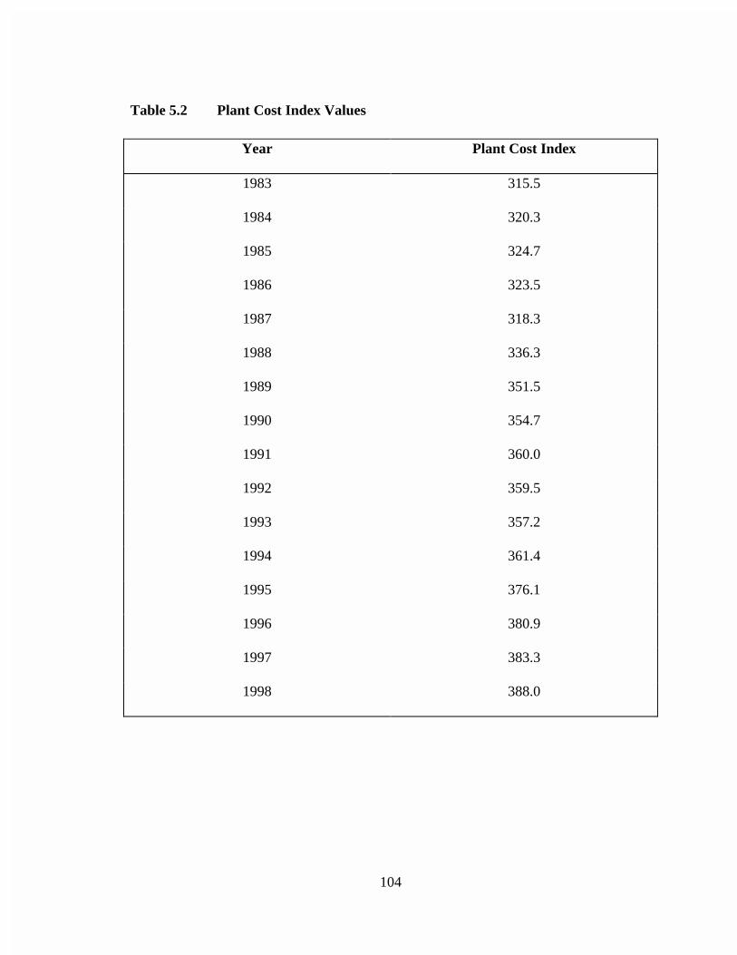
104
Table 5.2 Plant Cost Index Values
Year Plant Cost Index
1983 315.5
1984 320.3
1985 324.7
1986 323.5
1987 318.3
1988 336.3
1989 351.5
1990 354.7
1991 360.0
1992 359.5
1993 357.2
1994 361.4
1995 376.1
1996 380.9
1997 383.3
1998 388.0
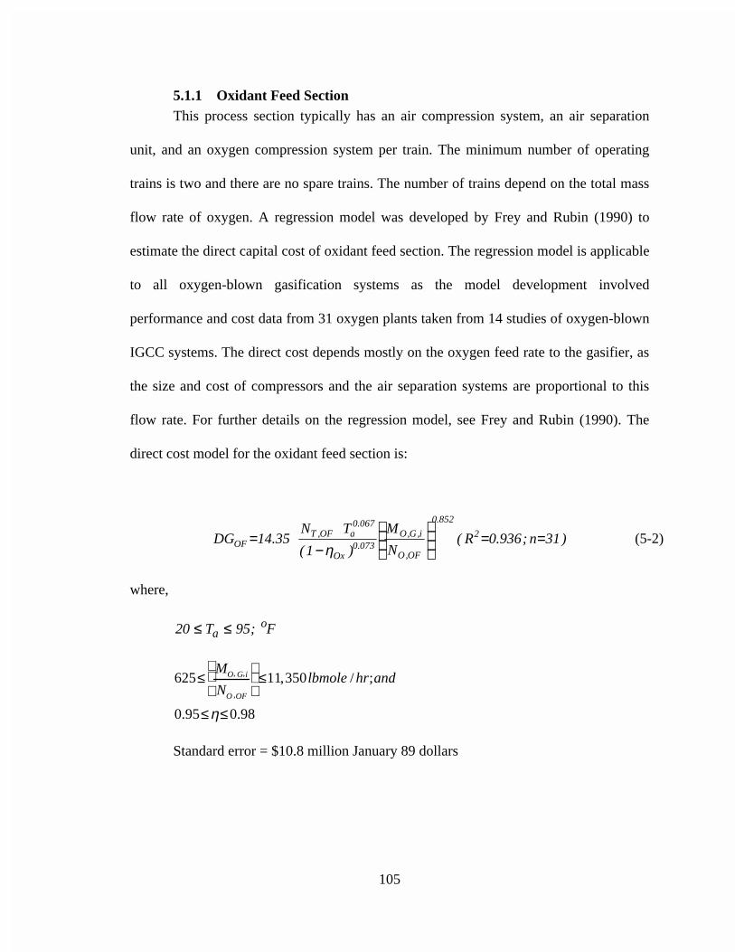
105
5.1.1 Oxidant Feed SectionThis process section typically has an air compression system, an air separation
unit, and an oxygen compression system per train. The minimum number of operating
trains is two and there are no spare trains. The number of trains depend on the total mass
flow rate of oxygen. A regression model was developed by Frey and Rubin (1990) to
estimate the direct capital cost of oxidant feed section. The regression model is applicable
to all oxygen-blown gasification systems as the model development involved
performance and cost data from 31 oxygen plants taken from 14 studies of oxygen-blown
IGCC systems. The direct cost depends mostly on the oxygen feed rate to the gasifier, as
the size and cost of compressors and the air separation systems are proportional to this
flow rate. For further details on the regression model, see Frey and Rubin (1990). The
direct cost model for the oxidant feed section is:
)31n;936.0R(N
M
)1(
TN35.14DG 2
852.0
OF,O
i,G,O073.0
Ox
067.0aOF,T
OF ==
−
=η
(5-2)
where,
F;95T20 oa ≤≤
625≤MO, G,i
NO ,OF
≤ 11,350lbmole / hr;and
0.95≤η≤0.98
Standard error = $10.8 million January 89 dollars
106
5.1.2 Coal Handling Section and Slurry PreparationCoal handling involves unloading coal from a train, storing the coal, moving the
coal to the grinding mills, and feeding the gasifier with positive displacement pumps. A
typical coal handling section contains one operating train and no spare train. A train
consists of a bottom dump railroad car unloading hopper, vibrating feeders, conveyors,
belt scale, magnetic separator, sampling system, deal coal storage, stacker, reclaimer, as
well as some of type of dust suppression system. Two studies (McNamee and White,
1986; Matchak et al., 1984) assumed a double boom stacker and bucket wheel reclaimer
system. The studies by Smith and Heaven (1992) and Hager and Heaven (1990) assumed
a combined stacker reclaimer. Pietruszkiewicz et al. (1988) specified conveyors to
perform the stacking operation and a rotary plow feeder for the reclaim system.
Slurry preparation trains typically have one to five operating trains with one spare
train. The typical train consists of vibrating feeders, conveyors, belt scale, rod mills,
storage tanks, and positive displacement pumps to feed the gasifiers. All of the equipment
for both the coal handling and the slurry feed are commercially available. This typical
train design is assumed in two reports (McNamee and White, 1986; Matchak et al.,
1984).
A regression model was developed for the direct capital cost of coal handling and
slurry preparation using the data collected for possible independent variables affecting
direct capital cost. The data sources are shown in Table 4.1 and Figure 5.1 shows the data
points. Coal feed rate to gasifier on as-received basis is the most common and easily
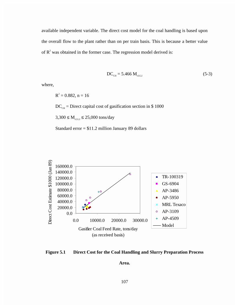
107
available independent variable. The direct cost model for the coal handling is based upon
the overall flow to the plant rather than on per train basis. This is because a better value
of R2 was obtained in the former case. The regression model derived is:
DCCH = 5.466 Mcf,G,I (5-3)
where,
R2 = 0.882, n = 16
DCCH = Direct capital cost of gasification section in $ 1000
3,300 ≤ Mcf,G,I ≤ 25,000 tons/day
Standard error = $11.2 million January 89 dollars
0.020000.040000.060000.080000.0
100000.0120000.0140000.0160000.0
0.0 10000.0 20000.0 30000.0
Gasifier Coal Feed Rate, tons/day (as received basis)
Dire
ct C
ost E
stim
ate
$100
0 (J
an 8
9)
TR-100319
GS-6904
AP-3486
AP-5950
MRL Texaco
AP-3109
AP-4509
Model
Figure 5.1 Direct Cost for the Coal Handling and Slurry Preparation Process
Area.
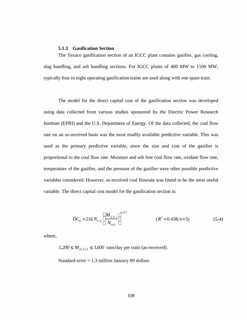
108
5.1.3 Gasification SectionThe Texaco gasification section of an IGCC plant contains gasifier, gas cooling,
slag handling, and ash handling sections. For IGCC plants of 400 MW to 1100 MW,
typically four to eight operating gasification trains are used along with one spare train.
The model for the direct capital cost of the gasification section was developed
using data collected from various studies sponsored by the Electric Power Research
Institute (EPRI) and the U.S. Department of Energy. Of the data collected, the coal flow
rate on an as-received basis was the most readily available predictive variable. This was
used as the primary predictive variable, since the size and cost of the gasifier is
proportional to the coal flow rate. Moisture and ash free coal flow rate, oxidant flow rate,
temperature of the gasifier, and the pressure of the gasifier were other possible predictive
variables considered. However, as-received coal flowrate was found to be the most useful
variable. The direct capital cost model for the gasification section is:
DCG =216 NT ,G
Mcf ,G ,i
NO,G
0.677
(R2 =0.438; n=5) (5-4)
where,
600,1M200,1 I,G,cf ≤≤ tons/day per train (as-received).
Standard error = 1.3 million January 89 dollars
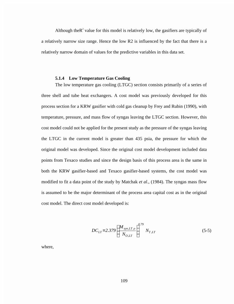
109
Although theR2 value for this model is relatively low, the gasifiers are typically of
a relatively narrow size range. Hence the low R2 is influenced by the fact that there is a
relatively narrow domain of values for the predictive variables in this data set.
5.1.4 Low Temperature Gas CoolingThe low temperature gas cooling (LTGC) section consists primarily of a series of
three shell and tube heat exchangers. A cost model was previously developed for this
process section for a KRW gasifier with cold gas cleanup by Frey and Rubin (1990), with
temperature, pressure, and mass flow of syngas leaving the LTGC section. However, this
cost model could not be applied for the present study as the pressure of the syngas leaving
the LTGC in the current model is greater than 435 psia, the pressure for which the
original model was developed. Since the original cost model development included data
points from Texaco studies and since the design basis of this process area is the same in
both the KRW gasifier-based and Texaco gasifier-based systems, the cost model was
modified to fit a data point of the study by Matchak et al., (1984). The syngas mass flow
is assumed to be the major determinant of the process area capital cost as in the original
cost model. The direct cost model developed is:
LT,T
79.0
LT,O
o,LT,synLT N
N
M379.2DC
= (5-5)
where,
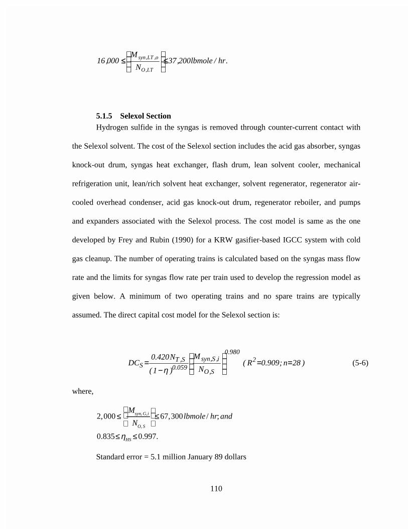
110
.hr/lbmole200,37N
M000,16
LT,O
o,LT,syn ≤
≤
5.1.5 Selexol SectionHydrogen sulfide in the syngas is removed through counter-current contact with
the Selexol solvent. The cost of the Selexol section includes the acid gas absorber, syngas
knock-out drum, syngas heat exchanger, flash drum, lean solvent cooler, mechanical
refrigeration unit, lean/rich solvent heat exchanger, solvent regenerator, regenerator air-
cooled overhead condenser, acid gas knock-out drum, regenerator reboiler, and pumps
and expanders associated with the Selexol process. The cost model is same as the one
developed by Frey and Rubin (1990) for a KRW gasifier-based IGCC system with cold
gas cleanup. The number of operating trains is calculated based on the syngas mass flow
rate and the limits for syngas flow rate per train used to develop the regression model as
given below. A minimum of two operating trains and no spare trains are typically
assumed. The direct capital cost model for the Selexol section is:
)28n;909.0R(N
M
)1(
N420.0DC 2
980.0
S,O
i,S,syn059.0
S,TS ==
−=
η(5-6)
where,
2,000 ≤Msyn, G,i
NO, S
≤67,300lbmole / hr; and
0.835≤ηHS ≤0.997.
Standard error = 5.1 million January 89 dollars
111
This model is valid for H2S removal efficiencies between 83.5 and 99.7 percent.
5.1.6 Claus Sulfur Recovery SectionThe Claus plant contains a two-stage sulfur furnace, sulfur condensers, and
catalysts. The cost model is same as the one developed by Frey and Rubin (1990). The
number of trains are estimated based on the recovered sulfur mass flow rate and the
allowable range of recovered sulfur mass flow rate per train used to develop the
regression model. The number of total trains is the number of operating trains and one
spare train. Typically, one or two operating trains are used. The direct capital cost model
as developed by Frey and Rubin (1990) is:
)21n;994.0R(N
MN28.6DC 2
668.0
C,O
o,C,sC,TC ==
= (5-7)
where,
hr/lbmole100,18N
M695
C,O
o,C,s ≤
≤
Standard error = 235,000 January 89 dollars
112
5.1.7 Beavon-Stretford Tail Gas Removal SectionThe capital cost of a Beavon-Stretford unit is expected to vary with the volume
flow rate of the input gas streams and with the mass flow rate of the sulfur produced. The
regression model developed by Frey and Rubin (1990) was based only on the sulfur
produced by the Beavon-Stretford process. The number of trains for this area is the same
as the number of trains for the Claus plant process area. The direct capital cost model for
this process area is:
)7n;998.0R(N
MN2.665.57DC 2
645.0
BS,O
o,BS,sBS,TBS ==
+= (5-8)
where,
200,1M75 o,BS,s ≤≤ lb/hr.
Standard error = 260,000 January 89 dollars
5.1.8 Boiler Feedwater SystemThe boiler feedwater system consists of equipment for handling raw water and
polished water in the steam cycle, including a water mineralization unit for raw water, a
dimineralized water storage tank, a condensate surge tank for storage of both
dimineralized raw water and steam turbine condensate water, a condensate polishing
unit., and a blowdown flash drum. The cost model, developed by Frey and Rubin (1990)
for a KRW gasifier-based IGCC system, considers both raw water flow rate through the
demineralization unit and the polished water flow rate through the polishing unit. The
polished water includes steam turbine condensate and makeup water, and condensate
113
from the miscellaneous process users such as waste water treatment. The number of trains
used for this commercially available process area is one, with no spare. The direct capital
cost model for this process area is:
)14n;991.0R(MM145.0DC 2435.0pw
307.0rwBFW === (5-9)
where,
000,614M000,24 rw ≤≤ lb/hr; and
000,880,3M000,234 pw ≤≤ lb/hr
5.1.9 Process Condensate TreatmentThe process condensate treatment area consists of strippers, air cooled heat
exchangers, and knock-out drums. It is expected that the process condensate treatment
direct cost will depend primarily on the scrubber blowdown flow rate, since the
blowdown from the gas scrubbing unit is the larger of the flow streams entering the
process condensate treatment section. The regression model developed for this process
area’s capital cost is:
DCPC =9700MSBD
300000
0.6
(5-10)
114
5.1.10 Gas Turbine SectionA number of design factors affect the cost of a gas turbine in an IGCC system. For
example, firing of medium-BTU coal gas, as opposed to high-BTU natural gas, requires
modification of the fuel nozzles and gas manifold in the gas turbine, which is designed
primarily for operating on natural gas. The gas turbine fuel inlet temperature is another
important design factor as low fuel inlet temperature may cause liquid condensation
leading to corrosion. The cost model for the gas turbine was developed for a GE Frame
7F gas turbine by Frey and Rubin (1990). In the model, the gross gas turbine electrical
input is estimated in MW. The number of gas turbines is estimated based on an
assumption of 190 MW output for each GE Frame 7F unit. There are no spare gas
turbines. The cost model is:
DCGT = 32000 NT,GT (5-11)
5.1.11 Heat Recovery Steam GeneratorThe heat recovery steam generator (HRSG) is a set of heat exchangers in which
heat is removed from the gas turbine exhaust gas to generate steam, including the
superheater, reheater, high pressure steam drum, high pressure evaporator, and the
economizers. The cost of the HRSG is expected to depend on factors such as the high
pressure steam flow rate to the steam turbine, the pressure of the steam, the gas turbine
exhaust gas volume flow rate, the number of steam drums, and, to a lesser extent, the
boiler feed water or saturated steam flow rates in each of the heat exchangers in the
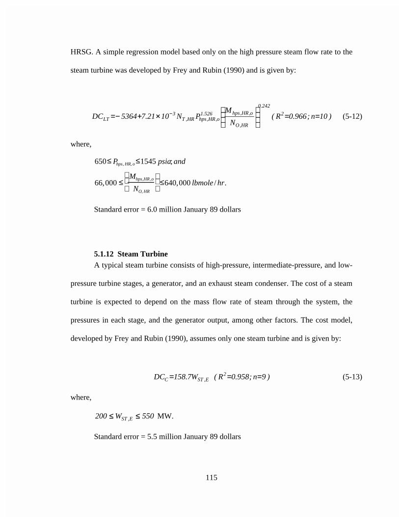
115
HRSG. A simple regression model based only on the high pressure steam flow rate to the
steam turbine was developed by Frey and Rubin (1990) and is given by:
)10n;966.0R(N
MPN1021.75364DC 2
242.0
HR,O
o,HR,hps526.1o,HR,hpsHR,T
3LT ==
×+−= − (5-12)
where,
650≤ Phps, HR, o ≤1545 psia; and
66,000 ≤Mhps,HR ,o
NO, HR
≤640,000 lbmole / hr.
Standard error = 6.0 million January 89 dollars
5.1.12 Steam TurbineA typical steam turbine consists of high-pressure, intermediate-pressure, and low-
pressure turbine stages, a generator, and an exhaust steam condenser. The cost of a steam
turbine is expected to depend on the mass flow rate of steam through the system, the
pressures in each stage, and the generator output, among other factors. The cost model,
developed by Frey and Rubin (1990), assumes only one steam turbine and is given by:
)9n;958.0R(W7.158DC 2E,STC === (5-13)
where,
550W200 E,ST ≤≤ MW.
Standard error = 5.5 million January 89 dollars
116
5.1.13 General FacilitiesThe general facilities section includes cooling water systems, plant and instrument
air, potable and utility water, and electrical system. Most studies assume that general
facilities are approximately 15 to 17 percent of direct costs (Frey and Rubin, 1990;
Matchak et al., 1984). In the present study the direct cost of the general facilities is
assumed to be approximately 17 percent of the direct costs of the all the other process
sections and is given by:
GF = fGF DCii =1
12
∑ (5-14)
where,
fGF = 0.17.
5.2 Total Plant Costs
The total plant costs of an IGCC power plant include the process facilities capital
costs, indirect construction costs, engineering and home office fees, sales tax, allowances
for funds used during construction (AFDC), project contingency, and total process
contingencies.
The equations for the plant cost model are the same as those given in Frey and
Rubin (1990) and are not repeated here. However, the model is briefly described.
117
Indirect construction costs include worker benefits, supervision and administrative
labor, purchased and rented construction equipment, and construction facilities.
Engineering and home office fees include the costs associated with engineering, office
expenses, and fees or profit to the engineer. Sales tax cost is specific to the state where
the power plant is constructed and is estimated as the tax on material costs. AFDC is the
estimated debt and equity costs of capital funds necessary to finance the construction of
new facilities. Startup costs include one month of fixed operating costs and one month of
variable costs based on full plant capacity.
Process contingency is used in deterministic cost estimates to quantify the
expected increase in the capital cost of an advanced technology due to uncertainty in
performance and cost for the specific design application. Project contingency is used in
deterministic cost estimates to represent the expected increase in the capital cost estimate
that would result from a more detailed estimate for a specific project at a particular site.
5.3 Total Capital Requirement
The total capital requirement (TCR) includes the total plant investment, prepaid
royalties, spare parts inventory, preproduction (or startup) costs, inventory capital, initial
chemicals and ctatlyst charges, and land costs. The methodology for calculating TCR is
given in detail in Frey and Rubin (1990).
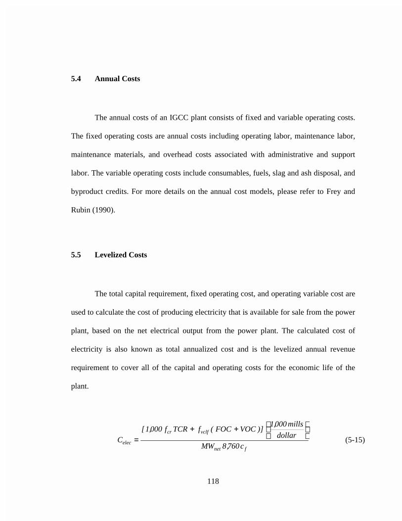
118
5.4 Annual Costs
The annual costs of an IGCC plant consists of fixed and variable operating costs.
The fixed operating costs are annual costs including operating labor, maintenance labor,
maintenance materials, and overhead costs associated with administrative and support
labor. The variable operating costs include consumables, fuels, slag and ash disposal, and
byproduct credits. For more details on the annual cost models, please refer to Frey and
Rubin (1990).
5.5 Levelized Costs
The total capital requirement, fixed operating cost, and operating variable cost are
used to calculate the cost of producing electricity that is available for sale from the power
plant, based on the net electrical output from the power plant. The calculated cost of
electricity is also known as total annualized cost and is the levelized annual revenue
requirement to cover all of the capital and operating costs for the economic life of the
plant.
fnet
vclfcr
elec c760,8MWdollar
mills000,1)]VOCFOC(fTCRf000,1[
C
++
= (5-15)
119
where,
Celec = The cost of electricity in mills per kWh
TCR = Total capital requirement in $1000
FOC = Fixed operating costs in dollars
VOC = Variable operating costs in dollars
MWnet = Net power output in MW
fcr = Fixed charge factor = 0.1034
fvclf = Variable levelization cost factor = 1.0
Cf = Capacity Factor = 0.65
120
6.0 APPLICATION OF THE PERFORMANCE, EMISSIONS, AND COSTMODEL OF THE COAL-FUELED IGCC SYSTEM WITH RADIANT ANDCONVECTIVE GAS COOLING TO A DETERMINISTIC CASE STUDY
An example case study is presented here to illustrate the use of the new IGCC
system model. The key steps in running the ASPEN simulation model of the Texaco
gasifier-based IGCC system are: (1) specify input assumptions; (2) execute the model;
(3) collect results; and (4) interpret the results.
6.1 Input Assumptions
Model input assumptions were developed for the performance and cost model
based upon a review of design and performance parameters obtained from literature (Frey
and Rubin, 1990; Frey and Rubin, 1991; Matchak et al., 1984; Farmer, 1997; Holt, 1998).
The assumed composition of the 3.9 weight percent (dry basis) sulfur Illinois No. 6 coal
is given in Table 3.1. The model is configured to represent three parallel trains of heavy
duty “Frame 7F” gas turbines.
Table 6.1 summarizes a number of the input assumptions for the example case study,
with a focus on the key inputs for the gasifier and gas turbine process areas of the model.
Many of these assumptions have been previously described in the technical description of
the technology. Two of the assumptions listed in the table are initial values that may be
121
modified during the simulation. These are the Oxygen/Coal ratio in the gasifier and the
Turbine Inlet Temperature in the gas turbine. The Oxygen/Coal ratio is varied by a design
specification in order to achieve the specified syngas exit temperature and overcome a
two percent heat loss from the gasifier. The Turbine Inlet Temperature may be lowered
from the initial value of 2,350 oF in order to maintain the exhaust gas temperature below
1,120 oF. There are literally hundreds of other input assumptions to the model. Only the
most significant ones affecting plant design and operation are shown here. The cost
model assumptions used in this case study are similar to those reported by Frey and
Rubin (1991).
6.2 Model Results
The version of ASPEN used in the present study is the one developed by US
Department of Energy. To execute the ASPEN model, an input file is prepared using
standard ASPEN keywords and is submitted to a multi-step process leading to model
execution. In the first step, the input file is translated into a FORTRAN program, which is
then compiled and linked to the extensive library of ASPEN unit operation and other
subroutines. The model is then executed and produces numerous output files. This
particular case study was executed on a VAX 4000 located at Carnegie Mellon
University, and the clock time for the run was approximately 5 minutes.
Selected performance and cost results from the model output are summarized in
Tables 6.2 and 6.3. The overall energy balance is indicated in Table 6.2. The plant is
122
estimated to produce a net of 863 MW with an overall plant efficiency of 39.4 percent on
a higher heating value basis. The breakdown of plant power production and internal plant
power consumption for auxiliaries is given in the Table 6.2. Buchanan et al. (1998)
mentions a first-of-a-kind (FOAK) IGCC plant which has a gasifier that closely
resembles the radiant and convective design adopted in the present study. The efficiency
of the FOAK plant is given to be 40.1 percent which is comparable to the efficiency
obtained by the current model. The FOAK plant produces 543 MW on a higher heating
value basis.
Estimated emission rates for SO2, NOx, particulate matter (PM), and CO2, are
provided in Table 6.2. SO2 emissions from IGCC systems are controlled by removing
sulfur species from the syngas prior to combustion in the gas turbine. NOx emissions tend
to be low for this particular IGCC system because there is very little fuel-bound nitrogen
in the fuel gas and thermal NO formation is low due to the low syngas heating value and
correspondingly relatively low adiabatic flame temperature. PM emissions are controlled
in the syngas cleanup system prior to the gas turbine. A primary purpose of the gas
cleanup system is to protect the gas turbine from contaminants in the fuel. Hence, no
post-combustion control is assumed. However, it is possible to further control NOx
emissions, for example, through use of Selective Catalytic Reduction (SCR) downstream
of the gas turbine. The emission rates of these pollutants are lower than for conventional
power plants and for many advanced coal-based power generation alternatives. CO2
emissions are lower than for conventional coal-fired power plants because of the higher
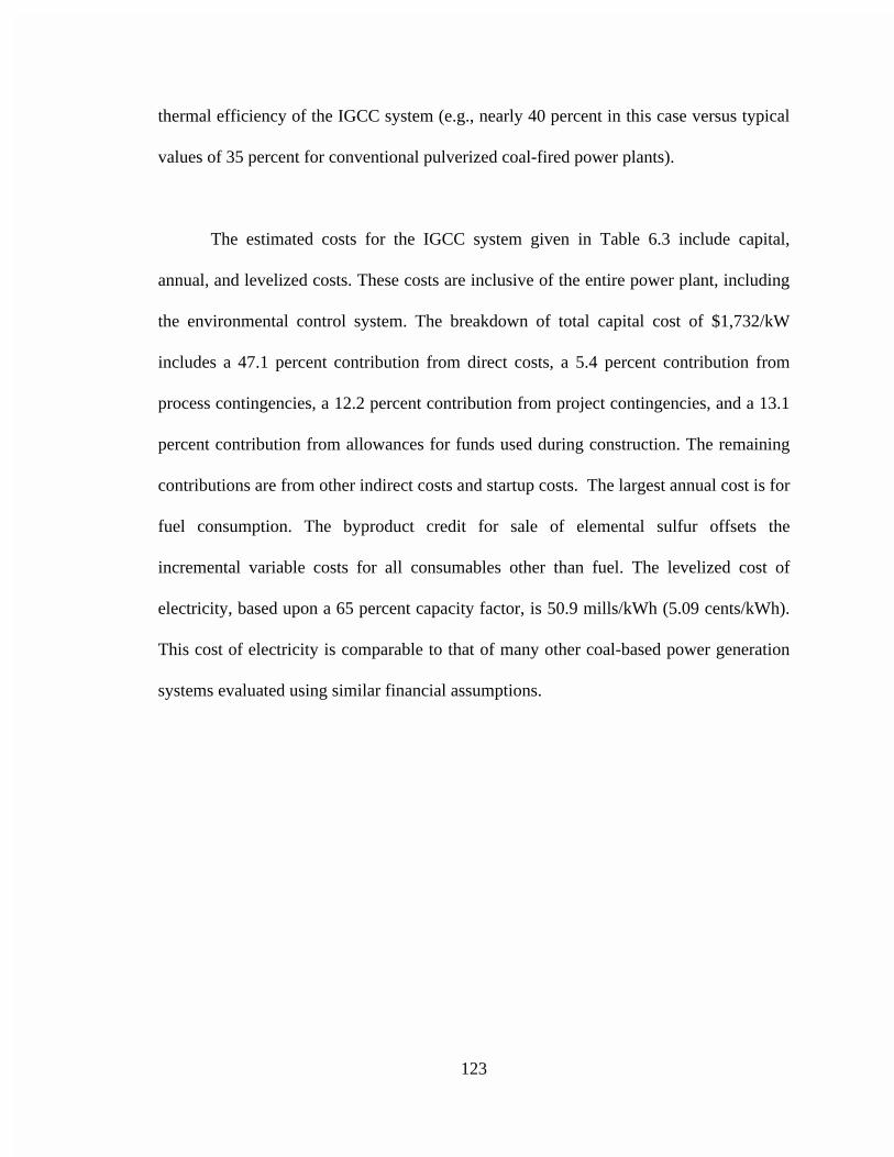
123
thermal efficiency of the IGCC system (e.g., nearly 40 percent in this case versus typical
values of 35 percent for conventional pulverized coal-fired power plants).
The estimated costs for the IGCC system given in Table 6.3 include capital,
annual, and levelized costs. These costs are inclusive of the entire power plant, including
the environmental control system. The breakdown of total capital cost of $1,732/kW
includes a 47.1 percent contribution from direct costs, a 5.4 percent contribution from
process contingencies, a 12.2 percent contribution from project contingencies, and a 13.1
percent contribution from allowances for funds used during construction. The remaining
contributions are from other indirect costs and startup costs. The largest annual cost is for
fuel consumption. The byproduct credit for sale of elemental sulfur offsets the
incremental variable costs for all consumables other than fuel. The levelized cost of
electricity, based upon a 65 percent capacity factor, is 50.9 mills/kWh (5.09 cents/kWh).
This cost of electricity is comparable to that of many other coal-based power generation
systems evaluated using similar financial assumptions.
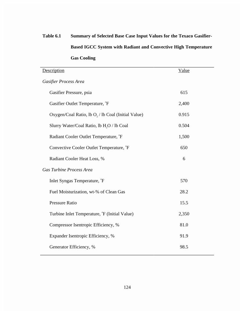
124
Table 6.1 Summary of Selected Base Case Input Values for the Texaco Gasifier-
Based IGCC System with Radiant and Convective High Temperature
Gas Cooling
Description Value
Gasifier Process Area
Gasifier Pressure, psia 615
Gasifier Outlet Temperature, oF 2,400
Oxygen/Coal Ratio, lb O2 / lb Coal (Initial Value) 0.915
Slurry Water/Coal Ratio, lb H2O / lb Coal 0.504
Radiant Cooler Outlet Temperature, oF 1,500
Convective Cooler Outlet Temperature, oF 650
Radiant Cooler Heat Loss, % 6
Gas Turbine Process Area
Inlet Syngas Temperature, oF 570
Fuel Moisturization, wt-% of Clean Gas 28.2
Pressure Ratio 15.5
Turbine Inlet Temperature, oF (Initial Value) 2,350
Compressor Isentropic Efficiency, % 81.0
Expander Isentropic Efficiency, % 91.9
Generator Efficiency, % 98.5
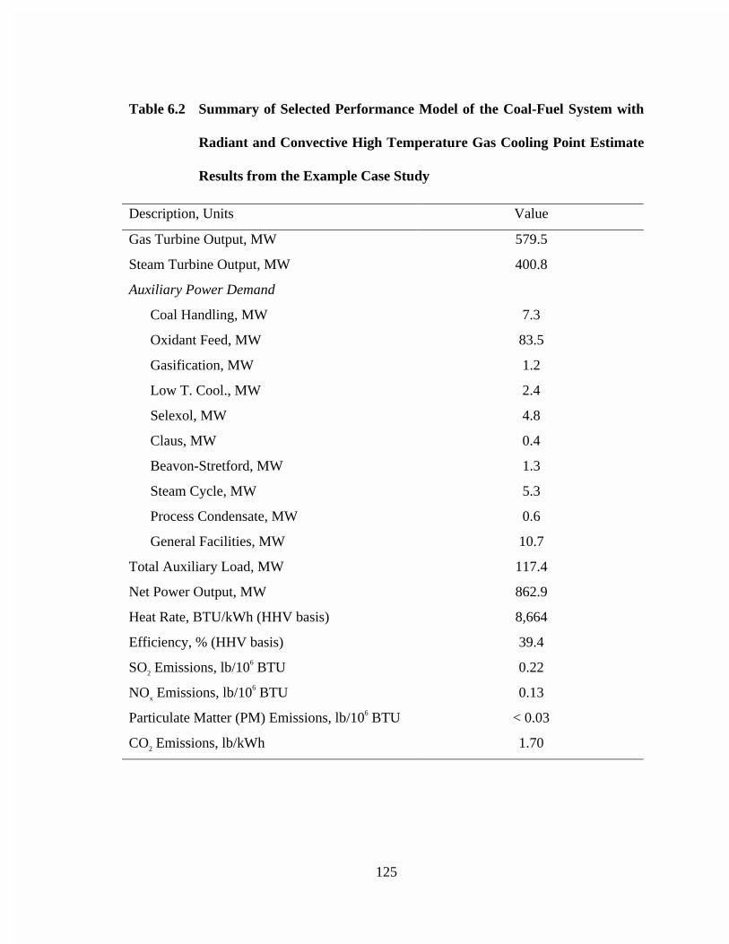
125
Table 6.2 Summary of Selected Performance Model of the Coal-Fuel System with
Radiant and Convective High Temperature Gas Cooling Point Estimate
Results from the Example Case Study
Description, Units Value
Gas Turbine Output, MW 579.5
Steam Turbine Output, MW 400.8
Auxiliary Power Demand
Coal Handling, MW 7.3
Oxidant Feed, MW 83.5
Gasification, MW 1.2
Low T. Cool., MW 2.4
Selexol, MW 4.8
Claus, MW 0.4
Beavon-Stretford, MW 1.3
Steam Cycle, MW 5.3
Process Condensate, MW 0.6
General Facilities, MW 10.7
Total Auxiliary Load, MW 117.4
Net Power Output, MW 862.9
Heat Rate, BTU/kWh (HHV basis) 8,664
Efficiency, % (HHV basis) 39.4
SO2 Emissions, lb/106 BTU 0.22
NOx Emissions, lb/106 BTU 0.13
Particulate Matter (PM) Emissions, lb/106 BTU < 0.03
CO2 Emissions, lb/kWh 1.70
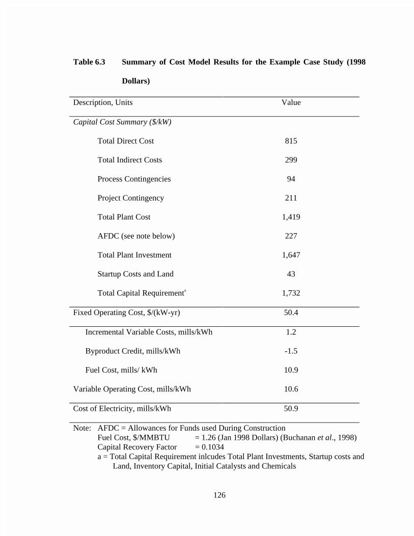
126
Table 6.3 Summary of Cost Model Results for the Example Case Study (1998
Dollars)
Description, Units Value
Capital Cost Summary ($/kW)
Total Direct Cost 815
Total Indirect Costs 299
Process Contingencies 94
Project Contingency 211
Total Plant Cost 1,419
AFDC (see note below) 227
Total Plant Investment 1,647
Startup Costs and Land 43
Total Capital Requirementa 1,732
Fixed Operating Cost, $/(kW-yr) 50.4
Incremental Variable Costs, mills/kWh 1.2
Byproduct Credit, mills/kWh -1.5
Fuel Cost, mills/ kWh 10.9
Variable Operating Cost, mills/kWh 10.6
Cost of Electricity, mills/kWh 50.9
Note: AFDC = Allowances for Funds used During ConstructionFuel Cost, $/MMBTU = 1.26 (Jan 1998 Dollars) (Buchanan et al., 1998)Capital Recovery Factor = 0.1034a = Total Capital Requirement inlcudes Total Plant Investments, Startup costs and
Land, Inventory Capital, Initial Catalysts and Chemicals
127
7.0 DOCUMENTATION OF THE PLANT PERFORMANCE, EMISSIONS,AND COST SIMULATION MODEL IN ASPEN OF THE COAL-FUELEDTEXACO-GASIFIER BASED IGCC SYSTEM WITH TOTAL QUENCHHIGH TEMPERATURE GAS COOLING
The performance model of an oxygen-blown Texaco gasifier based IGCC system
with total quench high temperature gas cooling (referred to here as the "total quench
model") is documented in this chapter. The development of the model is based primarily
on the findings of a study conducted by Electric Power Research Institute (Matchak et al.,
1984). This design is adopted as it provides extensive information on the mass flows of
streams, temperatures, pressures, power production and consumption, and costs
associated with each process section of the plant. Most of the major process sections are
modeled in similar method as for the radiant and convective method. Tables and figures
are listed for those process areas which are modeled differently from those in the radiant
and convective Texaco gasifier-based IGCC system. The convergence sequence for the
present model is described along with the FORTRAN blocks and design specifications
used in the model.
7.1 Major Process Sections in the Total Quench IGCC Process Simulation Model
Most of the major flowsheet sections in the process simulation model of the total
quench-based system, such as coal slurry preparation, gasification, particulate scrubbing,
acid gas removal, Claus sulfur recovery, Beavon-Stretford tail gas treatment, and gas
turbine, are similar in design to those in the radiant and convective-based model. The
128
flowsheet sections in the total quench model that are significantly different from their
counterparts in the radiant and convective design which are the high temperature gas
cooling section, low temperature gas cooling section, fuel gas saturation, and steam cycle,
are described below. The other process are modeled in the same manner as descibed in
Chapter 3.
7.1.1 Gasification and High Temperature Gas Cooling
Figure 7.1, and Table 7.1 illustrate the structure and input assumptions of the
gasification and high temperature gas cooling models. The gasification process is similar
to that in the radiant and convective design. The crude gas leaving the gasificaton unit is
at a temperature of 2400 oF to 2600 oF. As shown in Figure 7.1, the hot gas is introduced
directly into a water quench chamber located below the gasifier vessel. In the model, the
hot gas is simulated by the stream RXROUT. RXROUT enters the unit operation block
QUENMIX, which simulates a mixer. Quench water and the hot gas from the block
GASIFIER are mixed in QUENMIX. The resulting output stream, modeled by
QUENGAS, flows to the unit operation block QUENHEAT which simulates a heater.
QUENHEAT cools the QUENGAS stream to a temperature of 433 oF.
A design specification, SETQUEN, is used for setting the temperature of the
output stream from the QUENHEAT block. The mass flow of the quench water,
represented by QUWATER, is varied until the temperature of the stream represented by
COOLGAS is 433 oF. The quenched gas is sent to the particulate removal section.

129
The other components of this process area, such as the blocks SLURPUMP,
COALCONV, MAKESOOT, MAKESLAG, and SLAGOUT, are the same as described
in Chapter 3.0.
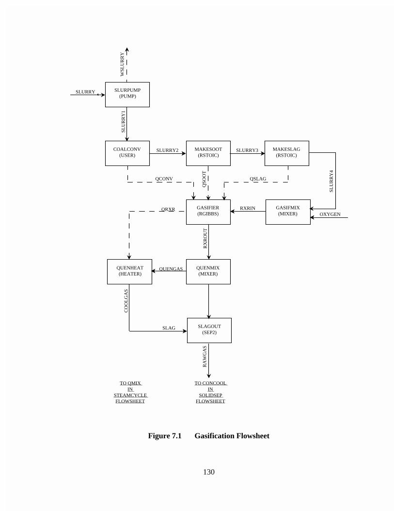
130
SLURPUMP (PUMP)
COALCONV (USER)
MAKESOOT (RSTOIC)
MAKESLAG (RSTOIC)
GASIFIER (RGIBBS)
GASIFMIX (MIXER)
QUENMIX (MIXER)
QUENHEAT (HEATER)
SLAGOUT (SEP2)
TO CONCOOL IN
SOLIDSEP FLOWSHEET
TO QMIX IN
STEAMCYCLE FLOWSHEET
SLURRY
WSL
UR
RY
SLU
RR
Y1
SLURRY2 SLURRY3
SLU
RR
Y4
QCONV
QSO
OT
QSLAG
QUENGAS
OXYGENRXRIN
RX
RO
UT
QRXR
CO
OL
GA
S
SLAG
RA
WG
AS
Figure 7.1 Gasification Flowsheet
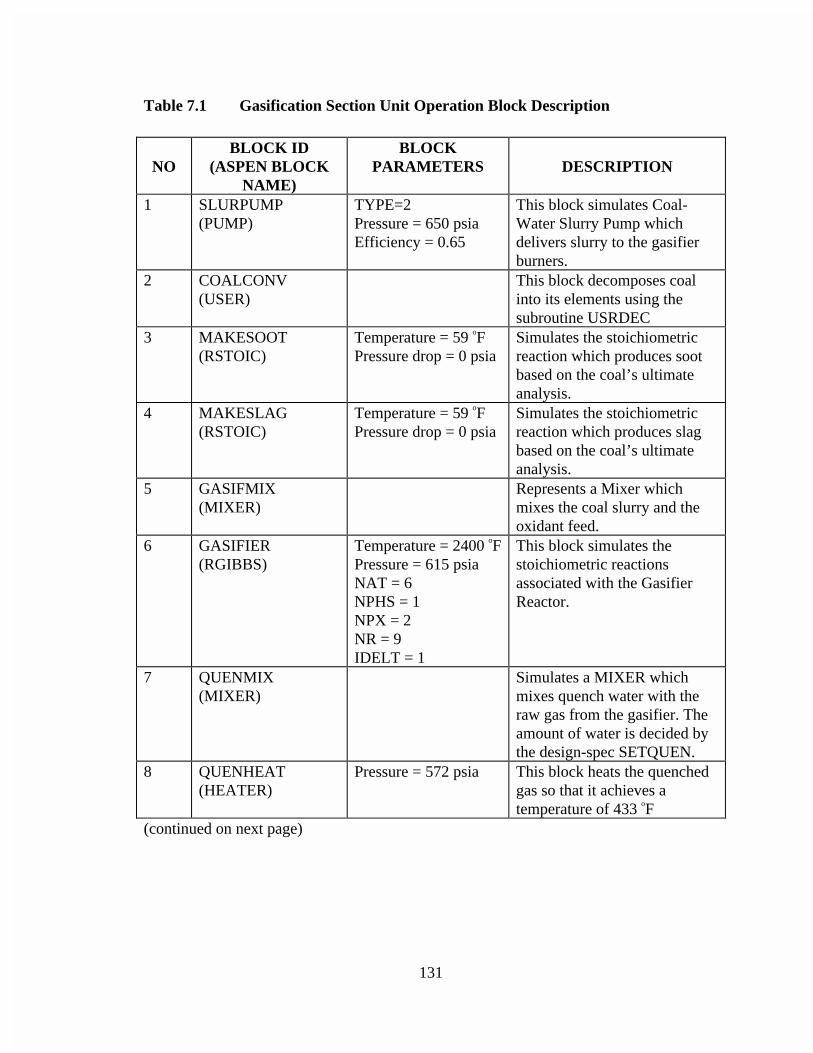
131
Table 7.1 Gasification Section Unit Operation Block Description
NOBLOCK ID
(ASPEN BLOCKNAME)
BLOCKPARAMETERS DESCRIPTION
1 SLURPUMP(PUMP)
TYPE=2Pressure = 650 psiaEfficiency = 0.65
This block simulates Coal-Water Slurry Pump whichdelivers slurry to the gasifierburners.
2 COALCONV(USER)
This block decomposes coalinto its elements using thesubroutine USRDEC
3 MAKESOOT(RSTOIC)
Temperature = 59 oFPressure drop = 0 psia
Simulates the stoichiometricreaction which produces sootbased on the coal’s ultimateanalysis.
4 MAKESLAG(RSTOIC)
Temperature = 59 oFPressure drop = 0 psia
Simulates the stoichiometricreaction which produces slagbased on the coal’s ultimateanalysis.
5 GASIFMIX(MIXER)
Represents a Mixer whichmixes the coal slurry and theoxidant feed.
6 GASIFIER(RGIBBS)
Temperature = 2400 oFPressure = 615 psiaNAT = 6NPHS = 1NPX = 2NR = 9IDELT = 1
This block simulates thestoichiometric reactionsassociated with the GasifierReactor.
7 QUENMIX(MIXER)
Simulates a MIXER whichmixes quench water with theraw gas from the gasifier. Theamount of water is decided bythe design-spec SETQUEN.
8 QUENHEAT(HEATER)
Pressure = 572 psia This block heats the quenchedgas so that it achieves atemperature of 433 oF
(continued on next page)
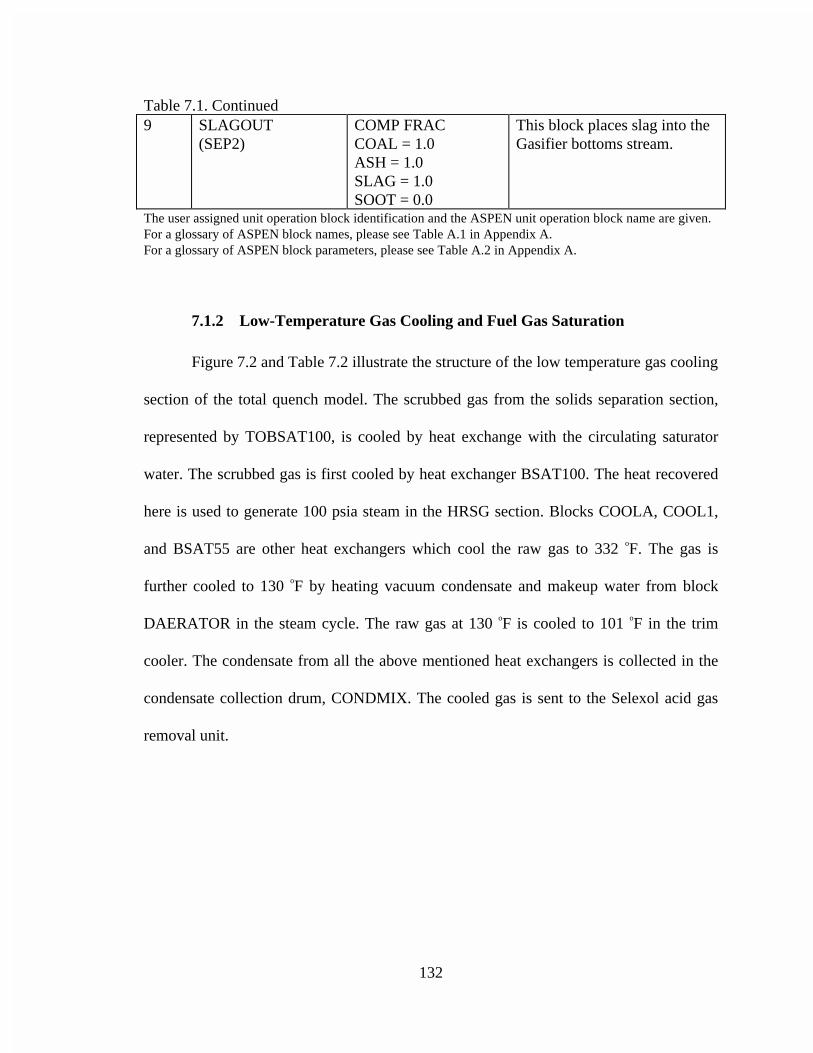
132
Table 7.1. Continued9 SLAGOUT
(SEP2)COMP FRACCOAL = 1.0ASH = 1.0SLAG = 1.0SOOT = 0.0
This block places slag into theGasifier bottoms stream.
The user assigned unit operation block identification and the ASPEN unit operation block name are given.For a glossary of ASPEN block names, please see Table A.1 in Appendix A.For a glossary of ASPEN block parameters, please see Table A.2 in Appendix A.
7.1.2 Low-Temperature Gas Cooling and Fuel Gas Saturation
Figure 7.2 and Table 7.2 illustrate the structure of the low temperature gas cooling
section of the total quench model. The scrubbed gas from the solids separation section,
represented by TOBSAT100, is cooled by heat exchange with the circulating saturator
water. The scrubbed gas is first cooled by heat exchanger BSAT100. The heat recovered
here is used to generate 100 psia steam in the HRSG section. Blocks COOLA, COOL1,
and BSAT55 are other heat exchangers which cool the raw gas to 332 oF. The gas is
further cooled to 130 oF by heating vacuum condensate and makeup water from block
DAERATOR in the steam cycle. The raw gas at 130 oF is cooled to 101 oF in the trim
cooler. The condensate from all the above mentioned heat exchangers is collected in the
condensate collection drum, CONDMIX. The cooled gas is sent to the Selexol acid gas
removal unit.
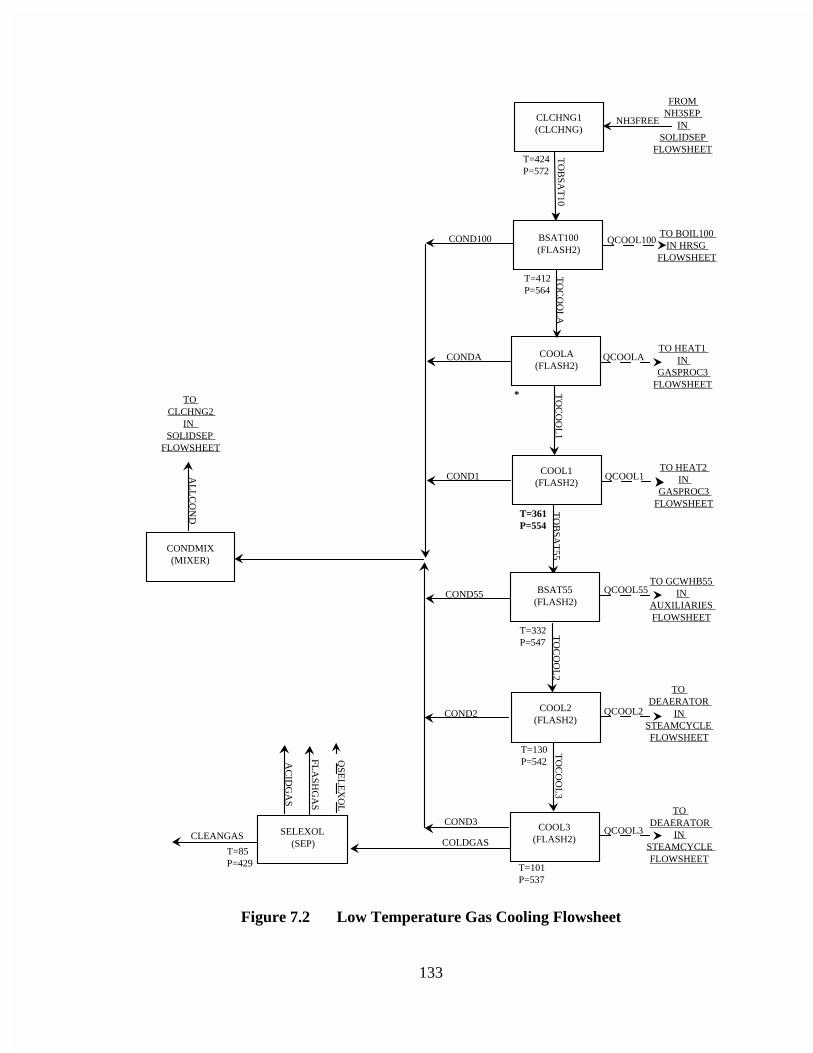
133
CLCHNG1 (CLCHNG)
COOL1 (FLASH2)
COOL2 (FLASH2)
COOL3 (FLASH2)
CONDMIX (MIXER)
FROM NH3SEP
IN SOLIDSEP
FLOWSHEET
TO CLCHNG2
IN SOLIDSEP
FLOWSHEET
NH3FREE
QCOOL1
TO
CO
OL
2T
OC
OO
L3
COLDGAS
AL
LC
ON
D
CLEANGAS
QSE
LE
XO
L
AC
IDG
AS
FLA
SHG
AS
TO
CO
OL
1
BSAT100 (FLASH2)
TO
BSA
T10
COOLA (FLASH2)
TO
CO
OL
A
BSAT55 (FLASH2)
TO
BSA
T55
TO HEAT2 IN
GASPROC3 FLOWSHEET
QCOOLATO HEAT1
IN GASPROC3
FLOWSHEET
QCOOL100TO BOIL100
IN HRSG FLOWSHEET
QCOOL55TO GCWHB55
IN AUXILIARIES FLOWSHEET
QCOOL2
TO DEAERATOR
IN STEAMCYCLE FLOWSHEET
QCOOL3
TO DEAERATOR
IN STEAMCYCLE FLOWSHEET
COND100
CONDA
COND1
COND55
COND2
COND3SELEXOL
(SEP)
T=424 P=572
T=412 P=564
*
T=361 P=554
T=332 P=547
T=130 P=542
T=101 P=537
T=85 P=429
Figure 7.2 Low Temperature Gas Cooling Flowsheet
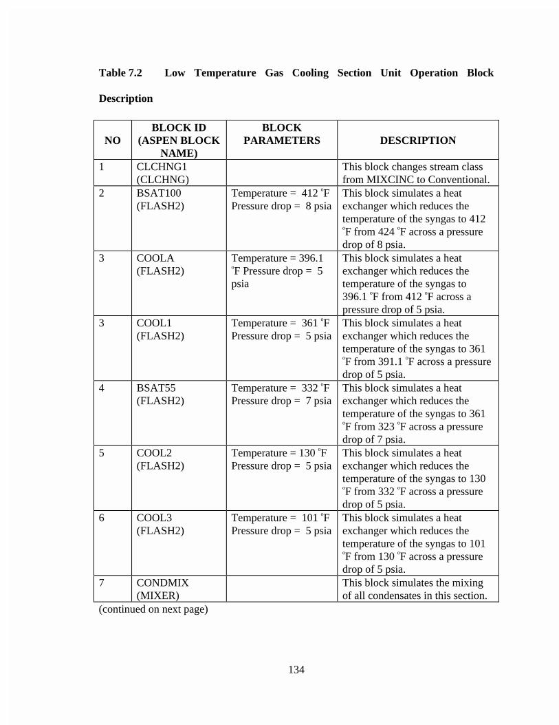
134
Table 7.2 Low Temperature Gas Cooling Section Unit Operation Block
Description
NOBLOCK ID
(ASPEN BLOCKNAME)
BLOCKPARAMETERS DESCRIPTION
1 CLCHNG1(CLCHNG)
This block changes stream classfrom MIXCINC to Conventional.
2 BSAT100(FLASH2)
Temperature = 412 oFPressure drop = 8 psia
This block simulates a heatexchanger which reduces thetemperature of the syngas to 412oF from 424 oF across a pressuredrop of 8 psia.
3 COOLA(FLASH2)
Temperature = 396.1oF Pressure drop = 5psia
This block simulates a heatexchanger which reduces thetemperature of the syngas to396.1 oF from 412 oF across apressure drop of 5 psia.
3 COOL1(FLASH2)
Temperature = 361 oFPressure drop = 5 psia
This block simulates a heatexchanger which reduces thetemperature of the syngas to 361oF from 391.1 oF across a pressuredrop of 5 psia.
4 BSAT55(FLASH2)
Temperature = 332 oFPressure drop = 7 psia
This block simulates a heatexchanger which reduces thetemperature of the syngas to 361oF from 323 oF across a pressuredrop of 7 psia.
5 COOL2(FLASH2)
Temperature = 130 oFPressure drop = 5 psia
This block simulates a heatexchanger which reduces thetemperature of the syngas to 130oF from 332 oF across a pressuredrop of 5 psia.
6 COOL3(FLASH2)
Temperature = 101 oFPressure drop = 5 psia
This block simulates a heatexchanger which reduces thetemperature of the syngas to 101oF from 130 oF across a pressuredrop of 5 psia.
7 CONDMIX(MIXER)
This block simulates the mixingof all condensates in this section.
(continued on next page)
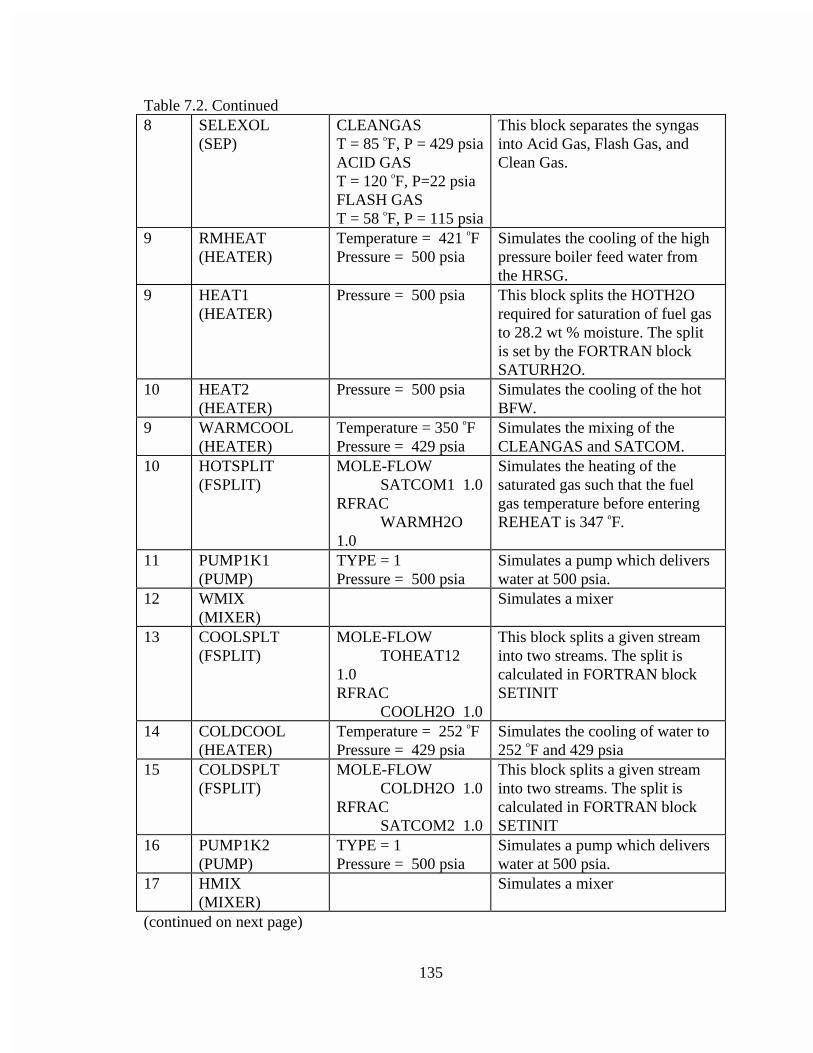
135
Table 7.2. Continued8 SELEXOL
(SEP)CLEANGAST = 85 oF, P = 429 psiaACID GAST = 120 oF, P=22 psiaFLASH GAST = 58 oF, P = 115 psia
This block separates the syngasinto Acid Gas, Flash Gas, andClean Gas.
9 RMHEAT(HEATER)
Temperature = 421 oFPressure = 500 psia
Simulates the cooling of the highpressure boiler feed water fromthe HRSG.
9 HEAT1(HEATER)
Pressure = 500 psia This block splits the HOTH2Orequired for saturation of fuel gasto 28.2 wt % moisture. The splitis set by the FORTRAN blockSATURH2O.
10 HEAT2(HEATER)
Pressure = 500 psia Simulates the cooling of the hotBFW.
9 WARMCOOL(HEATER)
Temperature = 350 oFPressure = 429 psia
Simulates the mixing of theCLEANGAS and SATCOM.
10 HOTSPLIT(FSPLIT)
MOLE-FLOW SATCOM1 1.0RFRAC WARMH2O1.0
Simulates the heating of thesaturated gas such that the fuelgas temperature before enteringREHEAT is 347 oF.
11 PUMP1K1(PUMP)
TYPE = 1Pressure = 500 psia
Simulates a pump which deliverswater at 500 psia.
12 WMIX(MIXER)
Simulates a mixer
13 COOLSPLT(FSPLIT)
MOLE-FLOW TOHEAT121.0RFRAC COOLH2O 1.0
This block splits a given streaminto two streams. The split iscalculated in FORTRAN blockSETINIT
14 COLDCOOL(HEATER)
Temperature = 252 oFPressure = 429 psia
Simulates the cooling of water to252 oF and 429 psia
15 COLDSPLT(FSPLIT)
MOLE-FLOW COLDH2O 1.0RFRAC SATCOM2 1.0
This block splits a given streaminto two streams. The split iscalculated in FORTRAN blockSETINIT
16 PUMP1K2(PUMP)
TYPE = 1Pressure = 500 psia
Simulates a pump which deliverswater at 500 psia.
17 HMIX(MIXER)
Simulates a mixer
(continued on next page)
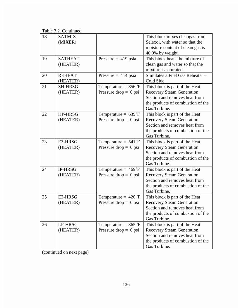
136
Table 7.2. Continued18 SATMIX
(MIXER)This block mixes cleangas fromSelexol, with water so that themoisture content of clean gas is40.0% by weight.
19 SATHEAT(HEATER)
Pressure = 419 psia This block heats the mixture ofclean gas and water so that themixture is saturated.
20 REHEAT(HEATER)
Pressure = 414 psia Simulates a Fuel Gas Reheater –Cold Side.
21 SH-HRSG(HEATER)
Temperature = 856 oFPressure drop = 0 psi
This block is part of the HeatRecovery Steam GenerationSection and removes heat fromthe products of combustion of theGas Turbine.
22 HP-HRSG(HEATER)
Temperature = 639 oFPressure drop = 0 psi
This block is part of the HeatRecovery Steam GenerationSection and removes heat fromthe products of combustion of theGas Turbine.
23 E3-HRSG(HEATER)
Temperature = 541 oFPressure drop = 0 psi
This block is part of the HeatRecovery Steam GenerationSection and removes heat fromthe products of combustion of theGas Turbine.
24 IP-HRSG(HEATER)
Temperature = 469 oFPressure drop = 0 psi
This block is part of the HeatRecovery Steam GenerationSection and removes heat fromthe products of combustion of theGas Turbine.
25 E2-HRSG(HEATER)
Temperature = 420 oFPressure drop = 0 psi
This block is part of the HeatRecovery Steam GenerationSection and removes heat fromthe products of combustion of theGas Turbine.
26 LP-HRSG(HEATER)
Temperature = 365 oFPressure drop = 0 psi
This block is part of the HeatRecovery Steam GenerationSection and removes heat fromthe products of combustion of theGas Turbine.
(continued on next page)
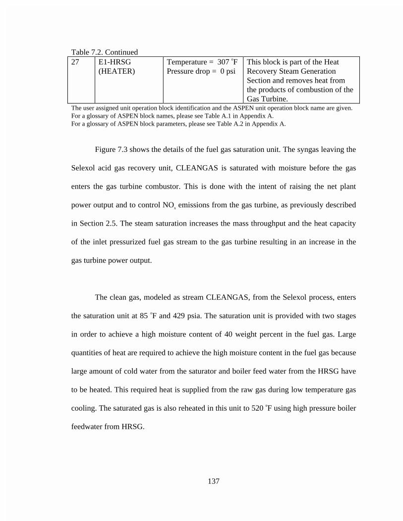
137
Table 7.2. Continued27 E1-HRSG
(HEATER)Temperature = 307 oFPressure drop = 0 psi
This block is part of the HeatRecovery Steam GenerationSection and removes heat fromthe products of combustion of theGas Turbine.
The user assigned unit operation block identification and the ASPEN unit operation block name are given.For a glossary of ASPEN block names, please see Table A.1 in Appendix A.For a glossary of ASPEN block parameters, please see Table A.2 in Appendix A.
Figure 7.3 shows the details of the fuel gas saturation unit. The syngas leaving the
Selexol acid gas recovery unit, CLEANGAS is saturated with moisture before the gas
enters the gas turbine combustor. This is done with the intent of raising the net plant
power output and to control NOx emissions from the gas turbine, as previously described
in Section 2.5. The steam saturation increases the mass throughput and the heat capacity
of the inlet pressurized fuel gas stream to the gas turbine resulting in an increase in the
gas turbine power output.
The clean gas, modeled as stream CLEANGAS, from the Selexol process, enters
the saturation unit at 85 oF and 429 psia. The saturation unit is provided with two stages
in order to achieve a high moisture content of 40 weight percent in the fuel gas. Large
quantities of heat are required to achieve the high moisture content in the fuel gas because
large amount of cold water from the saturator and boiler feed water from the HRSG have
to be heated. This required heat is supplied from the raw gas during low temperature gas
cooling. The saturated gas is also reheated in this unit to 520 oF using high pressure boiler
feedwater from HRSG.
138
The model of saturator for the total quench system is different from that described
in Section 2.5. Instead of direct contact of syngas with water, the heat transfer between
the clean syngas and the saturator water are modeled. The amount of water required to
saturate the clean syngas to 40 weight percent moisture is calcuated, and the heat required
to vaporize this amount of water is obtained from blocks HEAT1 and HEAT2. Finally,
the water vapor is mixed with the clean syngas and reheated in REHEATR before the
syngas is sent to the gas turbine. HEAT1 and HEAT2 simulate blocks which heat the
circulating water using heat recovered from unit operartion blocks COOLA and COOL1
respectively. WARMCOOL cools the hot water entering the saturator unit to an
intermediate temperature. The cooled hot water, HOTH21, is split into two streams,
WARMH2O and SATCOM1, by HOTSPLIT. PUMP1K1 is a pump, which increases the
pressure of WARMH2O to 500 psia. A mixer WMIX mixes the 500 psia WARMH2O
and the heated water from HEAT2. The mixed stream, TOSPLT, is split by COOLSPLT
into two streams, COOLH2O and TOHEAT12. The stream COOLH2O is cooled to a
temperature of 252 oF in block COLDCOOL, and split into COLDH2O and SATCOM2.
PUMP1K2 increases the pressure of COLDH2O to 500 psia before it is sent to HEAT2
block. TOHEAT12 is sent to the block HEAT1, where it is heated to become HOTW2.
CLEANGAS, SATCOM1, and SATCOM2 are mixed and heated to a temperature of 370
oF in the block SATHEAT. The high pressure boiler feedwater from the HRSG,
FGSMAK, is cooled to 421 oF by RMHEAT. The heat recovered from FGSMAK is used
to heat the saturated clean gas to 520 oF. The reheated fuel gas, GTFUEL flows to the gas
turbine combustors.
139
The saturation section flowsheet contains a FORTRAN block SETINIT which
calculates the required amount of water to be added to clean gas to make its moisture
content 40.0 percent by weight. SETINIT obtains the mass flow of clean gas entering the
saturator block and calculates mass flow of the saturated gas, SATGAS. The equation
used for this purpose is given by,
GasCleanwater M100
Mη
η−
= (7-1)
where,
Mwater = Mass flow of water to be added to the clean syngas, lb/hr
= SATCOM1 + SATCOM2
η = weight percent of moisture to be present in the saturated syngas
MCG = Mass flow of clean syngas from acid gas removal section (dry basis), lb/hr
The FORTRAN block SETINIT also calculates the split ratios for the blocks
HOTSPLIT and COLDSPLT using similar methods as in the FORTRAN block
SETSTEAM, elaborated upon in Section 3.2.6.3. SETINIT also sets the mass flow
makeup water to the steam cycle equal to the mass flow of water added to the clean
syngas.
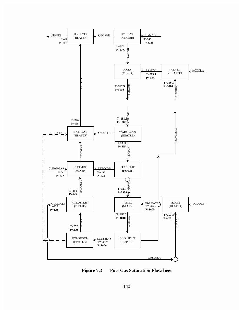
140
RMHEAT (HEATER)
FGSMAK
HO
TW
1
HMIX (MIXER)
TO
HE
AT
1
HOTW2 HEAT1 (HEATER)
QCOOLA
HO
TH
22
WARMCOOL (HEATER)
HO
TH
20H
OT
H21
HOTSPLIT (FSPLIT)
SATCOM1
WA
RM
H2O
WMIX (MIXER)
TO
HE
AT
2
FR-HEAT2 HEAT2 (HEATER)
QCOOL1
TO
SPLT
COOLSPLIT (FSPLIT)
TO
HE
AT
12
COOLH2OCOLDCOOL (HEATER)
CO
OL
H21
COLDSPLIT (FSPLIT)
SAT
CO
M2
SATMIX (MIXER)
CLEANGAS
QHEAT1SATHEAT (HEATER)
SAT
GA
S1
QHEAT2
SAT
GA
S
QTOREHREHEATR (HEATER)
GTFUEL
COLDH2O
COLDH2O
T=421 P=1000
T=549 P=1600
T=520 P=414
T=378 P=419
T=252 P=429
T=350 P=425
T=85 P=429
T=351.7 P=1000
T=350 P=425
T=381.5 P=1000
T=379.1 P=1000
T=252 P=429
T=253.2 P=429
T=346.5 P=1000
T=350.2 P=1000
T=252 P=429
T=382.5 P=1000
T=350.2 P=1000
T=349.9 P=1000
Figure 7.3 Fuel Gas Saturation Flowsheet
141
7.1.3 Steam Cycle
The steam cycle designed for the total quench model is similar to the one
designed for radiant and convective IGCC system except for a few differences. The
HRSG section in the total quench model has two extra economizers and an intermediate
pressure evaporator. The auxiliaries section has an additional 55 psia centrifugal pump
and a 55 psia steam boiler. The steam turbine section has only one low pressure (1 psia)
steam turbine unlike in the case of radiant and convective model in which there is also a
70 psia low pressure steam turbine. The rest of the steam cycle is the same as that
described in Section 3.2.6.
7.1.3.1 Heat Recovery Steam Generation (HRSG)
The operations of the HRSG are to preheat boiler feed water, reheat intermediate
pressure steam, supplement high pressure and 100 psia steam generation, and to superheat
high pressure steam. Figure 7.4 and Table 7.3 illustrate the model of the HRSG section.
The HRSG is arranged in the following order:
1. Superheater and reheater in parallel,
2. High pressure evaporator,
3. Economizer,
4. Intermediate pressure evaporator,
5. Economizer,
6. 100 psia boiler, and
142
7. Economizer.
Most of the HRSG section design is similar to the HRSG design in the radiant
and convective model. The key additions are ECONOMZ3, which models two
economizers, and the intermediate pressure boiler, IPBOILER, which generates saturated
steam of 350 psia. This steam is combined in the high pressure power turbine,
TURBREHT, with the high pressure steam (565 psia), STEAM565, from the Claus plant.
7.1.3.2 Auxiliaries Section
The auxiliaries section has similar design to that in the radiant and convective
model as shown in Figure 7.5 and Table 7.4. The key difference is the additional
generation of 55 psia steam by a waste heat boiler, GCWHB55 which is sent to the block
SPLIT55.
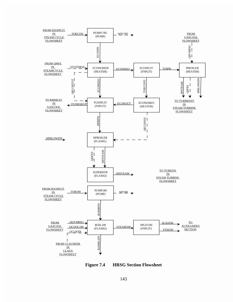
143
PUMP1785 (PUMP)
ECONOMZR (HEATER)
ECONOMZ3 (HEATER)
HPBOILER (FLASH2)
SUPERHTR (FLASH2)
PUMP180 (PUMP)
BOIL100 (FLASH2)
SPLIT100 (FSPLIT)
FGSSPLIT (FSPLIT)
ECOSPLIT (FSPLIT)
TO RMHEAT IN
GASCOOL FLOWSHEET
TO TURB350 IN
STEAM TURBINE FLOWSHEET
TO AUXILIARIES
SECTION
FROM GASCOOL
FLOWSHEET
FROM CLAUSRXR IN
CLAUS FLOWSHEET
FROM H2OSPLIT IN
STEAM CYCLE FLOWSHEET
FROM QMIX IN
STEAMCYCLE FLOWSHEET
TOECON
EC
ON
IN
QTOTHRSG
EC
ON
H2O
HPB
FW
QE
CO
NX
S
HPBLOWDN
TO
EC
ON
3
QH
PXS
HPS
TE
AM
SHSTEAM
TOB100 WP180
B10
0BF
WB
100B
LD
N
QLP-HRSG
QCLRXR
STEAM100SLXSTM
STM100
WP1785
FGSMAKUP
FROM H2OSPLIT IN
STEAM CYCLE FLOWSHEET
ECONH2OQ
EC
ON
TO
T
ECONOUT
TOIPB
QCOOL100
IPBOILER (HEATER)
FROM GASCOOL
FLOWSHEET
QIP
-HR
SG
IPST
EA
M
QIP
XS
IPB
LO
WD
N
TO TURBREHT IN
STEAM TURBINE FLOWSHEET
Figure 7.4 HRSG Section Flowsheet
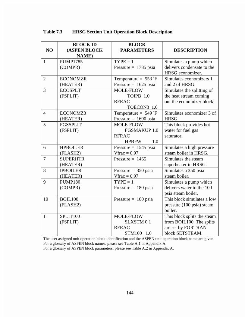
144
Table 7.3 HRSG Section Unit Operation Block Description
NOBLOCK ID
(ASPEN BLOCKNAME)
BLOCKPARAMETERS DESCRIPTION
1 PUMP1785(COMPR)
TYPE = 1Pressure = 1785 psia
Simulates a pump whichdelivers condensate to theHRSG economizer.
2 ECONOMZR(HEATER)
Temperature = 553 oFPressure = 1625 psia
Simulates economizers 1and 2 of HRSG.
3 ECOSPLT(FSPLIT)
MOLE-FLOW TOIPB 1.0RFRAC TOECON3 1.0
Simulates the splitting ofthe heat stream comingout the economizer block.
4 ECONOMZ3(HEATER)
Temperature = 549 oFPressure = 1600 psia
Simulates economizer 3 ofHRSG.
5 FGSSPLIT(FSPLIT)
MOLE-FLOW FGSMAKUP 1.0RFRAC HPBFW 1.0
This block provides hotwater for fuel gassaturator.
6 HPBOILER(FLASH2)
Pressure = 1545 psiaVfrac = 0.97
Simulates a high pressuresteam boiler in HRSG.
7 SUPERHTR(HEATER)
Pressure = 1465 Simulates the steamsuperheater in HRSG.
8 IPBOILER(HEATER)
Pressure = 350 psiaVfrac = 0.97
Simulates a 350 psiasteam boiler.
9 PUMP180(COMPR)
TYPE = 1Pressure = 180 psia
Simulates a pump whichdelivers water to the 100psia steam boiler.
10 BOIL100(FLASH2)
Pressure = 100 psia This block simulates a lowpressure (100 psia) steamboiler.
11 SPLIT100(FSPLIT)
MOLE-FLOW SLXSTM 0.1RFRAC STM100 1.0
This block splits the steamfrom BOIL100. The splitsare set by FORTRANblock SETSTEAM.
The user assigned unit operation block identification and the ASPEN unit operation block name are given.For a glossary of ASPEN block names, please see Table A.1 in Appendix A.For a glossary of ASPEN block parameters, please see Table A.2 in Appendix A.
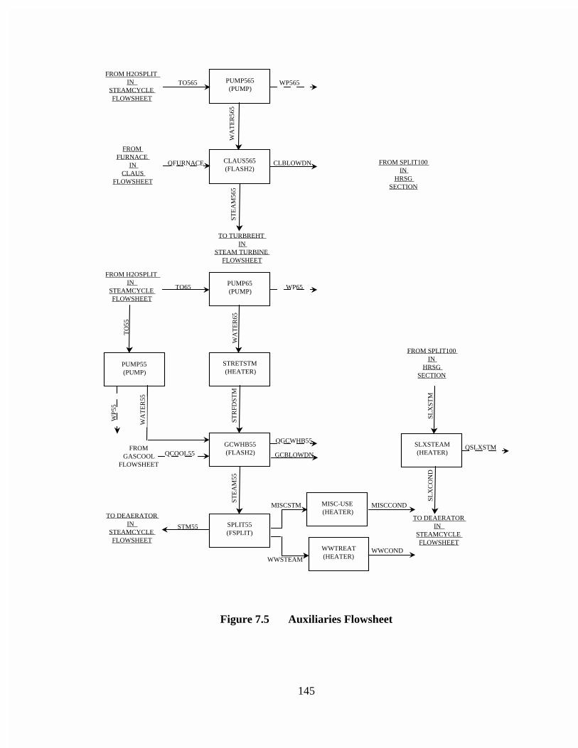
145
PUMP65 (PUMP)
PUMP565 (PUMP)
CLAUS565 (FLASH2)
STRETSTM (HEATER)
GCWHB55 (FLASH2)
SPLIT55 (FSPLIT)
MISC-USE (HEATER)
WWTREAT (HEATER)
SLXSTEAM (HEATER)
TO565
TO65 WP65
ST
EA
M56
5W
AT
ER
65ST
RFD
STM
GCBLOWDN
ST
EA
M55
STM55
MISCSTM
WWSTEAM
MISCCOND
WWCOND
SLX
STM
SL
XC
ON
D
QSLXSTM
WA
TE
R56
5
FROM SPLIT100 IN
HRSG SECTION
TO DEAERATOR IN
STEAMCYCLE FLOWSHEET
TO DEAERATOR IN
STEAMCYCLE FLOWSHEET
FROM SPLIT100 IN
HRSG SECTION
FROM H2OSPLIT IN
STEAMCYCLE FLOWSHEET
FROM H2OSPLIT IN
STEAMCYCLE FLOWSHEET
FROM FURNACE
IN CLAUS
FLOWSHEET
WP565
QFURNACE CLBLOWDN
TO TURBREHT IN
STEAM TURBINE FLOWSHEET
QGCWHB55
PUMP55 (PUMP)
TO
55
WA
TE
R55
WP
55
QCOOL55FROM
GASCOOL FLOWSHEET
Figure 7.5 Auxiliaries Flowsheet
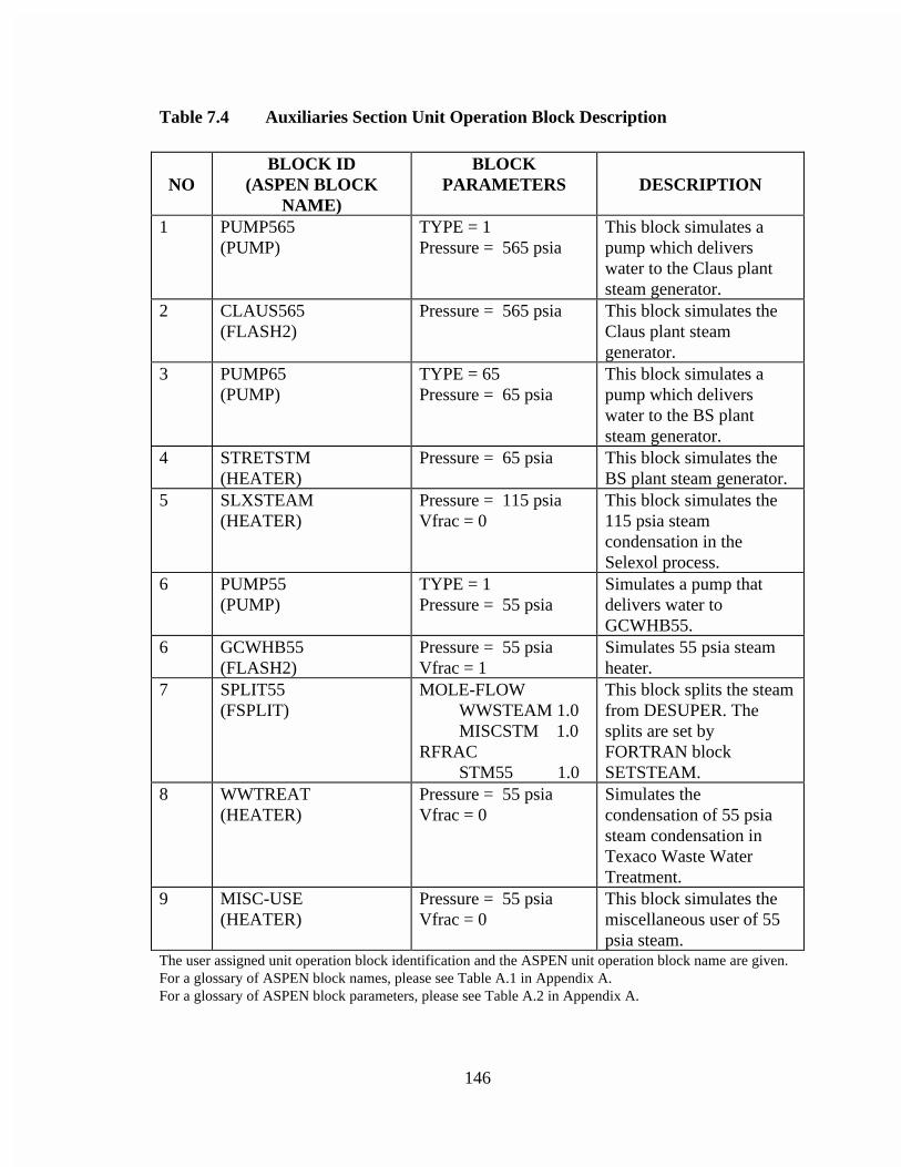
146
Table 7.4 Auxiliaries Section Unit Operation Block Description
NOBLOCK ID
(ASPEN BLOCKNAME)
BLOCKPARAMETERS DESCRIPTION
1 PUMP565(PUMP)
TYPE = 1Pressure = 565 psia
This block simulates apump which deliverswater to the Claus plantsteam generator.
2 CLAUS565(FLASH2)
Pressure = 565 psia This block simulates theClaus plant steamgenerator.
3 PUMP65(PUMP)
TYPE = 65Pressure = 65 psia
This block simulates apump which deliverswater to the BS plantsteam generator.
4 STRETSTM(HEATER)
Pressure = 65 psia This block simulates theBS plant steam generator.
5 SLXSTEAM(HEATER)
Pressure = 115 psiaVfrac = 0
This block simulates the115 psia steamcondensation in theSelexol process.
6 PUMP55(PUMP)
TYPE = 1Pressure = 55 psia
Simulates a pump thatdelivers water toGCWHB55.
6 GCWHB55(FLASH2)
Pressure = 55 psiaVfrac = 1
Simulates 55 psia steamheater.
7 SPLIT55(FSPLIT)
MOLE-FLOW WWSTEAM 1.0 MISCSTM 1.0RFRAC STM55 1.0
This block splits the steamfrom DESUPER. Thesplits are set byFORTRAN blockSETSTEAM.
8 WWTREAT(HEATER)
Pressure = 55 psiaVfrac = 0
Simulates thecondensation of 55 psiasteam condensation inTexaco Waste WaterTreatment.
9 MISC-USE(HEATER)
Pressure = 55 psiaVfrac = 0
This block simulates themiscellaneous user of 55psia steam.
The user assigned unit operation block identification and the ASPEN unit operation block name are given.For a glossary of ASPEN block names, please see Table A.1 in Appendix A.For a glossary of ASPEN block parameters, please see Table A.2 in Appendix A.
147
7.1.3.3 Steam Turbine
The details regarding the modeling of the steam turbine section are given in
Figure 7.6 and Table 7.5. Three steam turbines are modeled in this section: TURB350,
TURB90, and TURB1. The steam generated in the HRSG section is expanded through
these three turbine stages, consisting of a 350 psia pressure exhaust turbine followed by
an intermediate pressure turbine of exhaust pressure 90 psia, followed by a low pressure
(1 psia) exhaust turbine.
The superheated steam from the HRSG section, SHSTEAM enters the block
TURB350, which simulates a 350 psia steam turbine. The output stream of TURB350,
STEAM350 is mixed in the block TURBREHT with the stream STEAM565 from the
auxiliaries section and stream IPSTEAM from the HRSG section. The output stream of
TURBREHT, HOTSTEAM is sent to intermediate pressure (90 psia) steam turbine,
TURB90. The stream STEAM90 from TURB90 flows to the low pressure steam turbine,
TURB1 generating 1 psia steam which flows to the block CONDENSR in the steam
cycle flowsheet The work streams, WT350, WT90, and WT1 are summed to estimate the
shaft power input to the generator.
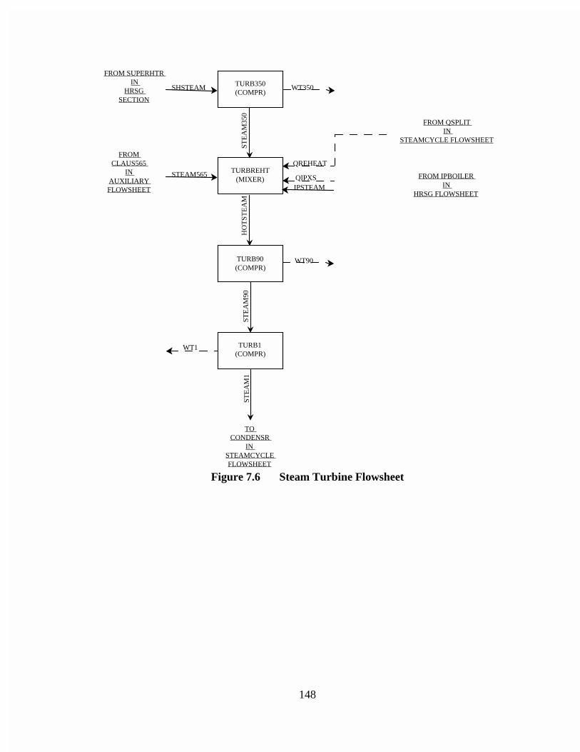
148
TURB350 (COMPR)
TURBREHT (MIXER)
TURB90 (COMPR)
TURB1 (COMPR)
FROM SUPERHTR IN
HRSG SECTION
FROM CLAUS565
IN AUXILIARY FLOWSHEET
FROM QSPLIT IN
STEAMCYCLE FLOWSHEET
TO CONDENSR
IN STEAMCYCLE FLOWSHEET
SHSTEAM WT350
STEAM565
STE
AM
90ST
EA
M1
WT1
WT90
HO
TST
EA
M
QREHEAT
STE
AM
350
FROM IPBOILER IN
HRSG FLOWSHEET
QIPXSIPSTEAM
Figure 7.6 Steam Turbine Flowsheet
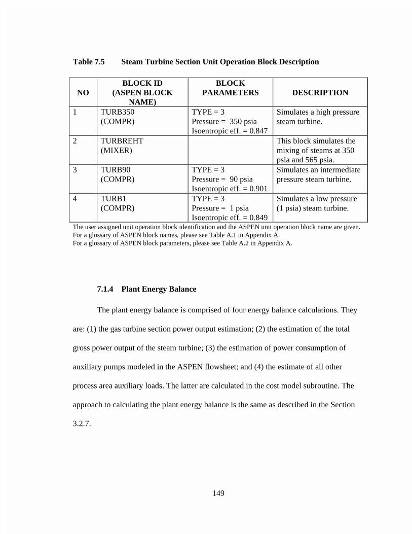
149
Table 7.5 Steam Turbine Section Unit Operation Block Description
NOBLOCK ID
(ASPEN BLOCKNAME)
BLOCKPARAMETERS DESCRIPTION
1 TURB350(COMPR)
TYPE = 3Pressure = 350 psiaIsoentropic eff. = 0.847
Simulates a high pressuresteam turbine.
2 TURBREHT(MIXER)
This block simulates themixing of steams at 350psia and 565 psia.
3 TURB90(COMPR)
TYPE = 3Pressure = 90 psiaIsoentropic eff. = 0.901
Simulates an intermediatepressure steam turbine.
4 TURB1(COMPR)
TYPE = 3Pressure = 1 psiaIsoentropic eff. = 0.849
Simulates a low pressure(1 psia) steam turbine.
The user assigned unit operation block identification and the ASPEN unit operation block name are given.For a glossary of ASPEN block names, please see Table A.1 in Appendix A.For a glossary of ASPEN block parameters, please see Table A.2 in Appendix A.
7.1.4 Plant Energy Balance
The plant energy balance is comprised of four energy balance calculations. They
are: (1) the gas turbine section power output estimation; (2) the estimation of the total
gross power output of the steam turbine; (3) the estimation of power consumption of
auxiliary pumps modeled in the ASPEN flowsheet; and (4) the estimate of all other
process area auxiliary loads. The latter are calculated in the cost model subroutine. The
approach to calculating the plant energy balance is the same as described in the Section
3.2.7.
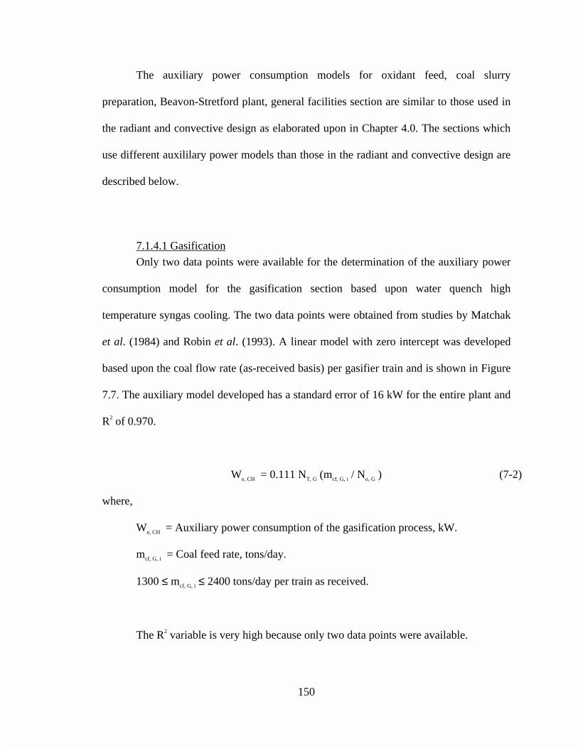
150
The auxiliary power consumption models for oxidant feed, coal slurry
preparation, Beavon-Stretford plant, general facilities section are similar to those used in
the radiant and convective design as elaborated upon in Chapter 4.0. The sections which
use different auxililary power models than those in the radiant and convective design are
described below.
7.1.4.1 Gasification
Only two data points were available for the determination of the auxiliary power
consumption model for the gasification section based upon water quench high
temperature syngas cooling. The two data points were obtained from studies by Matchak
et al. (1984) and Robin et al. (1993). A linear model with zero intercept was developed
based upon the coal flow rate (as-received basis) per gasifier train and is shown in Figure
7.7. The auxiliary model developed has a standard error of 16 kW for the entire plant and
R2 of 0.970.
We, CH = 0.111 NT, G (mcf, G, i / No, G ) (7-2)
where,
We, CH = Auxiliary power consumption of the gasification process, kW.
mcf, G, i = Coal feed rate, tons/day.
1300 ≤ mcf, G, i ≤ 2400 tons/day per train as received.
The R2 variable is very high because only two data points were available.
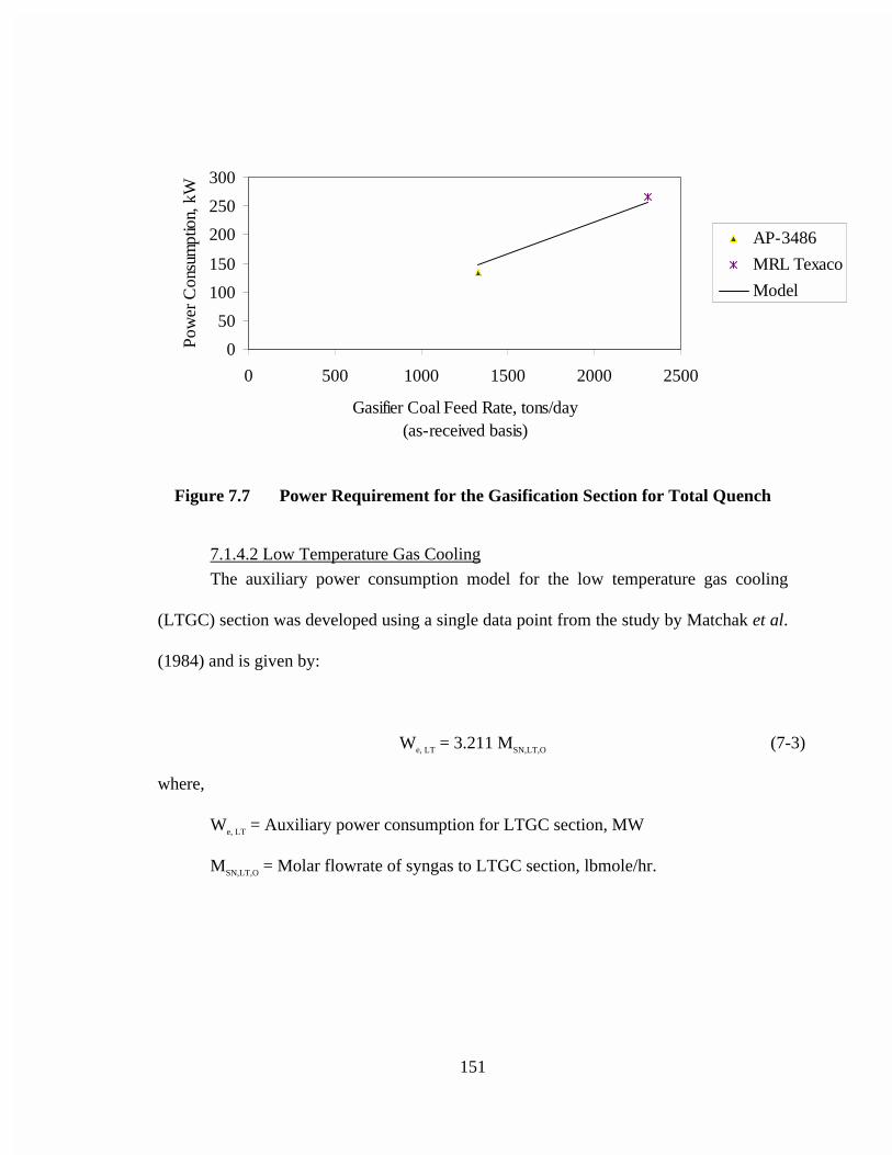
151
0
50
100
150
200
250
300
0 500 1000 1500 2000 2500
Gasifier Coal Feed Rate, tons/day(as-received basis)
Pow
er C
onsu
mpt
ion,
kW
AP-3486
MRL Texaco
Model
Figure 7.7 Power Requirement for the Gasification Section for Total Quench
7.1.4.2 Low Temperature Gas Cooling
The auxiliary power consumption model for the low temperature gas cooling
(LTGC) section was developed using a single data point from the study by Matchak et al.
(1984) and is given by:
We, LT = 3.211 MSN,LT,O (7-3)
where,
We, LT = Auxiliary power consumption for LTGC section, MW
MSN,LT,O = Molar flowrate of syngas to LTGC section, lbmole/hr.
152
7.1.4.3 Selexol
The auxiliary power consumption model for the Selexol section was developed as
part of the current study using a single data point from the study by Matchak et al. (1984)
The auxiliary power consumption model for Selexol process in MW is given by
We, S = 2.07 x 10⁻⁵ Msyn,S,I (7-4)
where,
MSYN,S,I = Molar flow rate of syngas entering Selexol process, lbmole/hr.
7.1.4.4 Claus Plant
The auxiliary power consumption model for the Claus plant was developed as part
of the current study using a single data point from the study by Matchak et al. (1984) The
auxiliary power consumption model for Claus plant in MW is given by
We, C = 1.4055 x 10⁻⁵ Ms,C,o (7-5)
where,
MS,C,O = Mass flow of sulfur from Claus plant, lb/hr.
7.1.4.5 Process Condensate Treatment
The process condensate treatment plant has the following auxiliary power
consumption model, which is developed for the present Texaco total quench gasification
system using a single data point from the study Matchat et al., (1984) and is given in MW
by the equation:
153
We, PC = 9.289 x 10⁻⁷ MS,BD (7-6)
where,
MS,BD = Scrubber blowdown flowrate, lb/hr.
7.2 Convergence Sequence
The convergence sequence for the total quench model simulation is similar to the
convergence sequence specified in the radiant and convective design as described in
Section 3.3. The additional blocks used for designing the total quench section of the
model replace the high temperature gas cooling section of the model containing the
radiant and convective design and the additional economizers in the total quench model
are added the convergence sequence developed for the radiant and convective model.
7.3 Environmental Emissions
NOX, particulate, SO2, and CO2 emissions are modeled in the same method as
done in the radiant and convective design.
154
7.4 Capital Cost Model
This section documents the cost model developed for the Texaco gasifier-based
IGCC plant with total quench high temperature gas cooling. New direct capital cost
models for major process sections are presented here. For the purpose of estimating the
direct capital costs of the plant, the IGCC plant is divided into thirteen process areas as
listed in Table 5.1. The direct cost of a process section can be adjusted for other years
using the appropriate Chemical Engineering Plant Cost Index (PCI) as shown in Table
5.2 and described in Section 5.1.
The direct capital cost models for coal handling section, oxidant feed section,
Claus recovery section, Beavon-Stretford plant, gas turbine, boiler feedwater system,
process condensate system, heat recovery steam generation system, steam turbine section,
and general facilities are the same as those in radiant and convective design for coal. The
process area direct capital costs for gasification, low temperature gas cooling, and Selexol
are different from those in the radiant and convective system and are described here.
7.4.1 Gasification SectionThe Texaco gasification section of an IGCC plant contains gas scrubbing, gas
cooling, slag handling, and ash handling. For IGCC plants of 400 MW to 1100 MW,
typically four to eight operating gasification trains are used along with one spare train
(Matchak et al., 1984).
155
Only two data points were available for the development of this cost model. The
data points are not conducive to cost model development using regression analysis, since
a straight line connecting them would have a negative slope. Therefore, a representative
value based upon the average of the two points is used to represent the direct cost of a
single gasifier train. A plot of the data is given Figure 7.8. From the two data points an
approximation was determined to be 10 million January dollars per train. Since the data
are based upon a coal feed rate of 1,300 to 2,300 tons/day (as-received basis), the average
cost is assumed to apply for individual trains in this size range. The direct capital cost in
January 1989 dollars for the gasification section is:
GTG NDC ,000,000,10= (7-7)
where,
NT,G = Number of trains
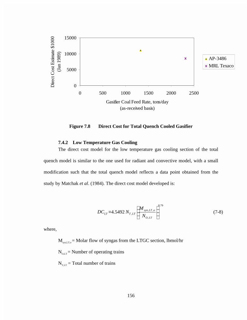
156
0
5000
10000
15000
0 500 1000 1500 2000 2500
Gasifier Coal Feed Rate, tons/day(as-received basis)
Dire
ct C
ost E
stim
ate
$100
0 (J
an 1
989)
AP-3486
MRL Texaco
Figure 7.8 Direct Cost for Total Quench Cooled Gasifier
7.4.2 Low Temperature Gas CoolingThe direct cost model for the low temperature gas cooling section of the total
quench model is similar to the one used for radiant and convective model, with a small
modification such that the total quench model reflects a data point obtained from the
study by Matchak et al. (1984). The direct cost model developed is:
79.0
,
,,,5492.4
=
LTO
oLTsynLTTLT N
MNDC (7-8)
where,
Msyn,LT,o = Molar flow of syngas from the LTGC section, lbmol/hr
NO,LT = Number of operating trains
NT,LT = Total number of trains
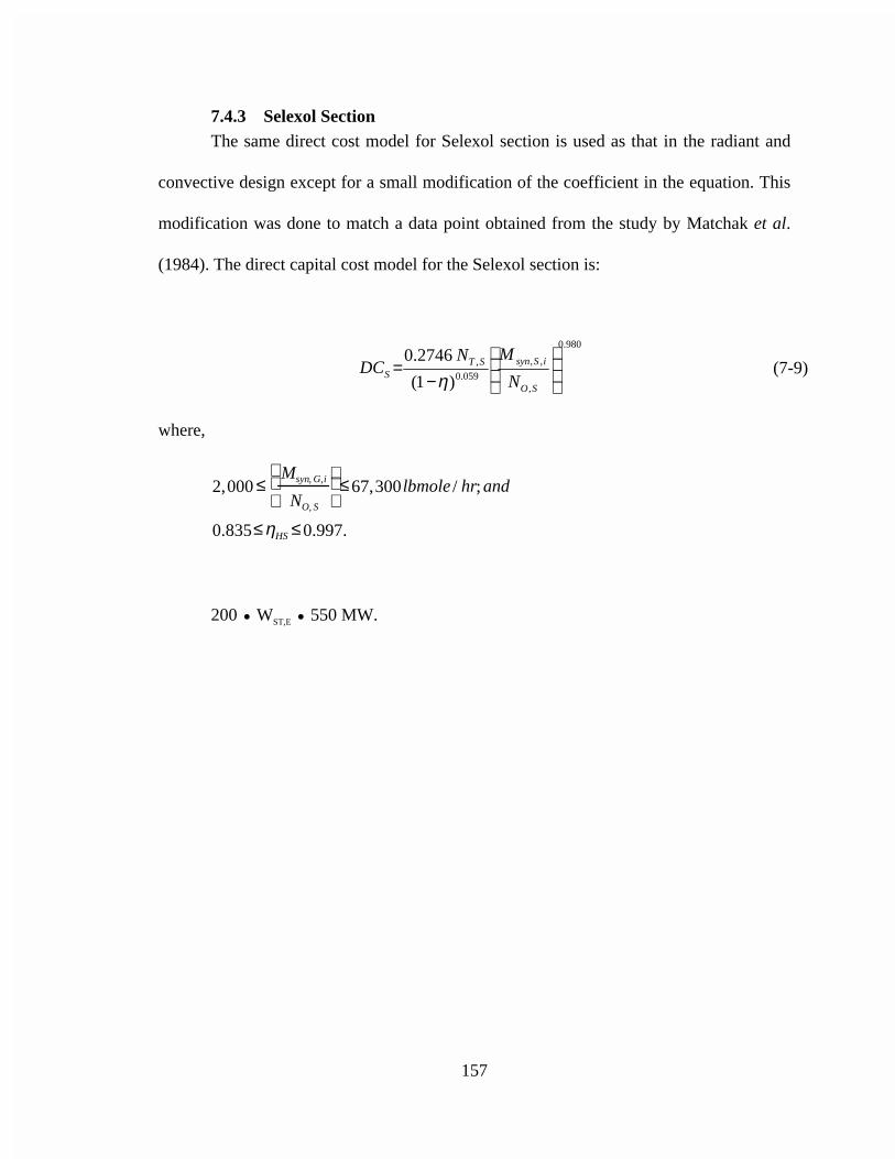
157
7.4.3 Selexol SectionThe same direct cost model for Selexol section is used as that in the radiant and
convective design except for a small modification of the coefficient in the equation. This
modification was done to match a data point obtained from the study by Matchak et al.
(1984). The direct capital cost model for the Selexol section is:
980.0
,
,,
059.0
,
)1(
2746.0
−
=SO
iSsynSTS N
MNDC
η(7-9)
where,
2,000 ≤Msyn, G,i
NO, S
≤67,300lbmole / hr; and
0.835≤ηHS ≤0.997.
200 • WST,E • 550 MW.
158
8.0 APPLICATION OF THE PERFORMANCE, EMISSIONS, AND COSTMODEL OF THE COAL-FUELED IGCC SYSTEM WITH TOTALQUENCH GAS COOLING TO A DETERMINISTIC CASE STUDY
An example case study is presented here to illustrate the use of the new IGCC
system model for the coal-fueled system with total quench high temperature gas cooling.
The key steps in running the ASPEN simulation model of the Texaco gasifier-based
IGCC system are: (1) specify input assumptions; (2) execute the model; (3) collect
results; and (4) interpret the results.
8.1 Input Assumptions
Model input assumptions were developed for the performance and cost model
similar to those developed for radiant and convective model. The model is configured to
represent three parallel trains of heavy duty “Frame 7F” gas turbines. Table 8.1
summarizes a number of the input assumptions for the example case study, with a focus
on the key inputs for the gasifier and gas turbine process areas of the model. Many of
these assumptions have been previously described in the technical description of the
technology. Two of the assumptions listed in the table are initial values that may be
modified during the simulation. These are the Oxygen/Coal ratio in the gasifier and the
Turbine Inlet Temperature in the gas turbine. The Oxygen/Coal ratio is varied by a design
specification in order to achieve the specified syngas exit temperature and overcome a
two percent heat loss from the gasifier. The Turbine Inlet Temperature may be lowered
159
from the initial value of 2,350 oF in order to maintain the exhaust gas temperature below
1,120 oF. There are literally hundreds of other input assumptions to the model. Only the
most significant ones affecting plant design and operation are shown here. The cost
model assumptions used in this case study are similar to those reported by Frey and
Rubin (1991).
8.2 Model Results
The version of ASPEN used in the present study is the one developed by US
Department of Energy. To execute the ASPEN model, an input file is prepared using
standard ASPEN keywords and is submitted to a multi-step process leading to model
execution. In the first step, the input file is translated into a FORTRAN program, which is
then compiled and linked to the extensive library of ASPEN unit operation and other
subroutines. The model is then executed and produces numerous output files. This
particular case study was executed on a VAX 4000 located at Carnegie Mellon
University, and the clock time for the run was about 5 minutes.
Selected performance and cost results from the model output are summarized in
Tables 8.2 and 8.3. The overall energy balance is indicated in Table 8.2. The plant is
estimated to produce a net of 793 MW with an overall plant efficiency of 35.0 percent on
a higher heating value basis. The breakdown of plant power production and internal plant
power consumption for auxiliaries is given in the Table 8.3.
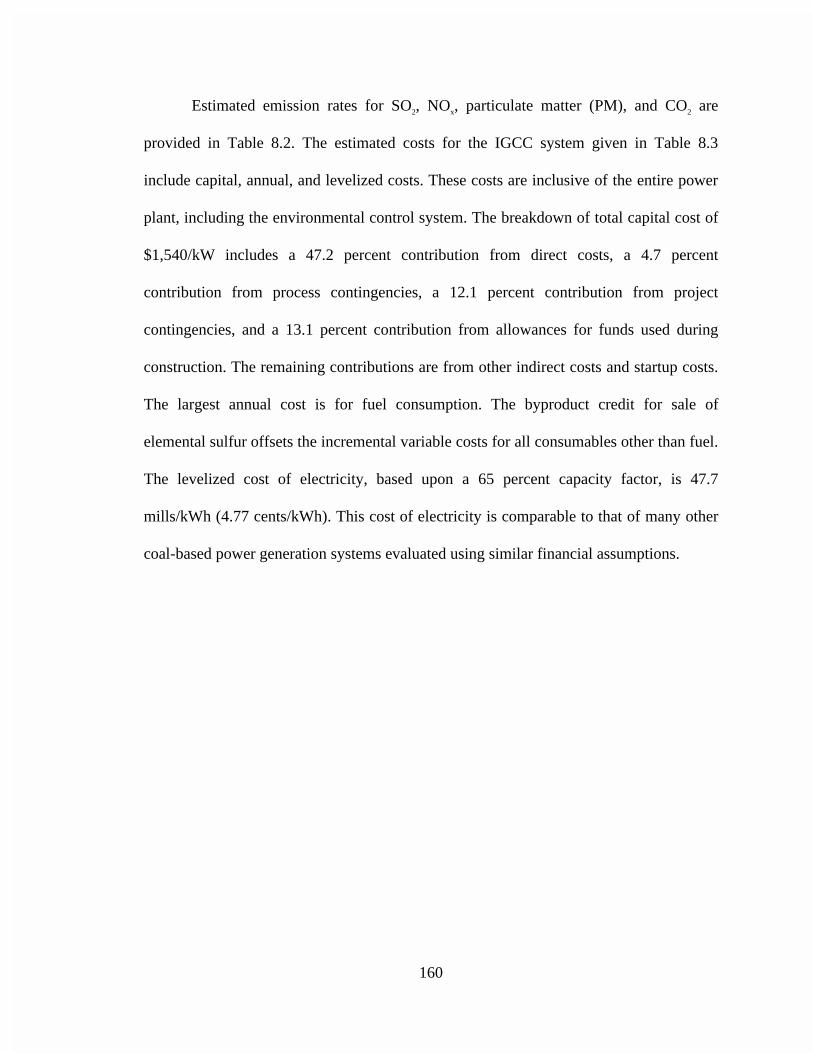
160
Estimated emission rates for SO2, NOx, particulate matter (PM), and CO2 are
provided in Table 8.2. The estimated costs for the IGCC system given in Table 8.3
include capital, annual, and levelized costs. These costs are inclusive of the entire power
plant, including the environmental control system. The breakdown of total capital cost of
$1,540/kW includes a 47.2 percent contribution from direct costs, a 4.7 percent
contribution from process contingencies, a 12.1 percent contribution from project
contingencies, and a 13.1 percent contribution from allowances for funds used during
construction. The remaining contributions are from other indirect costs and startup costs.
The largest annual cost is for fuel consumption. The byproduct credit for sale of
elemental sulfur offsets the incremental variable costs for all consumables other than fuel.
The levelized cost of electricity, based upon a 65 percent capacity factor, is 47.7
mills/kWh (4.77 cents/kWh). This cost of electricity is comparable to that of many other
coal-based power generation systems evaluated using similar financial assumptions.

161
Table 8.1 Summary of the Base Case Parameters Values for the Texaco Coal
Gasification Total Quench System
Description, Units Value
Gasifier Process Area
Gasifier Pressure, psia 615
Gasifier Outlet Temperature, oF 2,400
Oxygen/Coal Ratio, lb O2 / lb Coal (Initial Value) 0.915
Slurry Water/Coal Ratio, lb H2O / lb Coal 0.504
Quench Cooler Outlet Temperature, oF 433
Gas Turbine Process Area
Inlet Syngas Temperature, oF 526
Fuel Moisturization, wt-% of Clean Gas 40.0
Pressure Ratio 15.5
Turbine Inlet Temperature, oF (Initial Value) 2,350
Compressor Isentropic Efficiency, % 81.0
Expander Isentropic Efficiency, % 91.9
Generator Efficiency, % 98.5
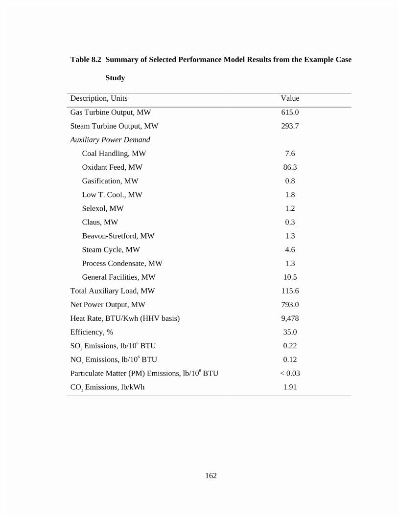
162
Table 8.2 Summary of Selected Performance Model Results from the Example Case
Study
Description, Units Value
Gas Turbine Output, MW 615.0
Steam Turbine Output, MW 293.7
Auxiliary Power Demand
Coal Handling, MW 7.6
Oxidant Feed, MW 86.3
Gasification, MW 0.8
Low T. Cool., MW 1.8
Selexol, MW 1.2
Claus, MW 0.3
Beavon-Stretford, MW 1.3
Steam Cycle, MW 4.6
Process Condensate, MW 1.3
General Facilities, MW 10.5
Total Auxiliary Load, MW 115.6
Net Power Output, MW 793.0
Heat Rate, BTU/Kwh (HHV basis) 9,478
Efficiency, % 35.0
SO2 Emissions, lb/106 BTU 0.22
NOx Emissions, lb/106 BTU 0.12
Particulate Matter (PM) Emissions, lb/106 BTU < 0.03
CO2 Emissions, lb/kWh 1.91
163
Table 8.3 Summary of Cost Model Results for the Example Case Study (1998
Dollars)
Description, Units Value
Capital Cost Summary ($/kW)
Total Direct Cost 728
Total Indirect Costs 267
Process Contingencies 73
Project Contingency 187
Total Plant Cost 1,256
AFDC (see note below) 201
Total Plant Investment 1,457
Startup Costs and Land 68
Total Capital Requirementa 1,540
Fixed Operating Cost, $/(kW-yr) 42.6
Incremental Variable Costs, mills/kWh 1.6
Byproduct Credit, mills/kWh 1.7
Fuel Cost, mills/ kWh 12.3
Variable Operating Cost, mills/kWh 12.2
Cost of Electricity, mills/kWh 47.7
Note: AFDC = Allowances for Funds used During ConstructionFuel Cost, $/MMBTU = 1.26 (Jan 1998 Dollars)Capital Recovery Factor = 0.1034a = Total Capital Requirement inlcudes Total Plant Investments, Startup costs and
Land, Inventory Capital, Initial Catalysts and Chemicals

164
165
9.0 UNCERTAINTY ANALYSIS
Process technologies that are still in the research phase are subject to uncertainty
with respect to prediction of performance, emissions, and costs. Insights into risks of such
new technologies are obtained by analyzing the uncertainties associated with them.
Uncertainty and sensitivity analysis of technology assessment models are done to find out
which assumptions and uncertainties may affect the conclusions significantly.
In any type of modeling effort, the limitations of data and of knowledge about the
system should be reflected in the model results. Uncertainties are prevalent in the early
stages of any technology development effort and hence must be incorporated in the
analysis and design of the technology. Uncertainty analysis has been described as “the
computation of the total uncertainty induced in the output by quantified uncertainty in
inputs and models, and the attributes of the relative importance of the input uncertainties
in terms of their contribution” (Morgan and Henrion, 1990). Incorporating uncertainties
in the development of new technology model helps in: (1) identifying robust solutions to
process design questions and to eliminate inferior design options; (2) identifying key
problems areas in a technology failure; (3) comparing competing technologies on a
consistent basis to determine the risks associated with adopting a new technology; and (4)
evaluating the effects that additional research might have on comparisons with
conventional technology (Frey and Rubin, 1991).
166
In probabilistic analysis, uncertainties in model input parameters are represented
using probability distributions. Using probabilistic simulation techniques, simultaneous
uncertainties in any number of model input parameters can be propagated through a
model to determine the combined effect on model outputs. The result of a probabilistic
simulation includes both the possible range of values for model output parameters and
information about the likelihood of obtaining various results. This provides insight into
risks and potential pay-offs of a new technology. Statistical analysis on the inputs and
output data can be used to identify trends without the need to re-run the analysis. Thus,
probabilistic analysis can be used to the identify the uncertainties in a process that matter
the most.
9.1 Methodology for Probabilistic Analysis
9.1.1 Characterizing Uncertainties
There are three general areas of uncertainty that should be explicitly reflected in
engineering models. There are uncertainties in: (1) process performance parameters (e.g.,
heat losses and removal efficiencies); (2) process area capital cost; and (3) process
operating cost (Frey and Rubin, 1992b). The approaches to developing probability
distributions for model input parameters are similar in many ways to the approach one
might take to pick a single “best guess” number for deterministic (point-estimate)
analysis or to select a range of values to use in sensitivity analysis. However, the
167
development of estimates of uncertainty usually requires more detailed thinking about
possible outcomes and their relative likelihoods.
The steps involved in estimating uncertainties for model input parameters are
(Frey and Rubin, 1992,a):
1. Review the technical basis for uncertainty in the process;
2. Identify candidate parameters that should be treated as uncertain;
3. Determine the sources of information regarding uncertainty for each
parameter; and
4. Develop estimates of uncertainty depending on the availability of
information.
Estimates of uncertainty in terms of ranges and probability distributions for model
input parameters can be based on: (1) published judgements in the literature; (2)
published information, both quantitative and qualitative, that can be used to infer a
judgement about uncertainty; (3) statistical analysis of data; and (4) judgements elicited
from technical experts with relevant expertise (Frey and Rubin, 1990; Morgan and
Herrion, 1990).
Probability distributions for uncertainty can be developed from available data
using statistical techniques. The data can be fitted to a particular distribution using
168
various statistical tests. When the data available are limited, engineering insight can be
used to supplement the data in coming up with an appropriate probability distribution for
the uncertain variable.
When sufficient data are not available, judgements from technical experts can be
elicited to obtain an appropriate probability distribution for the uncertain variable. In
designing elicitation protocol, it is important to take into account heuristics by which
judgements about uncertainty may be. Some heuristics can lead to biases in the
judgements. However, protocols can be designed to counteract these sources of bias.
9.1.2 Types of Uncertain Quantities
Many types of random variation should be considered in developing a probability
distribution for a variable. These are briefly discussed in Frey and Rubin (1991) and are
reviewed here.
9.1.2.1 Variability
Variability is caused due to variations in the process itself. For example, a
variation in the coal composition will cause a variation in the net efficiency of the plant.
Variability can be represented as a probability distribution.
169
9.1.2.2 Uncertainty
Uncertainty represents the lack of knowledge regarding the true value of a
quantity. There are a number of types of uncertainty which can be considered while
developing a probability distribution for a variable. Variability is conceptually distinct
from uncertainty (Frey and Rubin, 1992b). For example, for a given coal composition, the
carbon conversion may be uncertain.
1. Statistical Error – is associated with imperfections in measurement techniques.
Statistical analysis of test data is thus one method for developing a representation
of uncertainty in a variable.
2. Systematic Error – The mean value of a quantity may not converge to the “true”
mean value because of biases in measurement and procedures. Such biases may
arise from imprecise calibration, faulty reading of meters, and inaccuracies in the
assumptions used to infer the actual quantity of interest from the observed
readings of other quantities.
Uncertainty may also arise due to lack of experience with a process. This type of
uncertainty often cannot be treated statistically because it requires predictions about
something that has yet to be built or tested. This type of uncertainty can be represented
using technical estimates about the range and likelihood of possible outcomes.
170
9.1.3 Some Types of Probability Distributions
An expert may specify a judgement regarding uncertainties using different types
of probabilistic distributions. One way of representing a probability distribution is the
cumulative distribution function (CDF), which shows the probability fractiles on the y-
axis and the value of the fractile associated with each fractile on the x-axis. Some
commonly used probability distributions are shown in Figure 9.1.
1. Uniform - represents uniform probability of obtaining a value between upper and
lower limits.
2. Triangle - - represents uniform probability of obtaining a value between upper and
lower limits with values biased toward a modal value specified.
3. Normal – is a symmetric distribution with mean, mode, and median at the same
point. It is often assumed in statistical analysis as the basis for unbiased
measurement errors.
4. Lognormal – is a positively skewed distribution and has a long tail to the right.
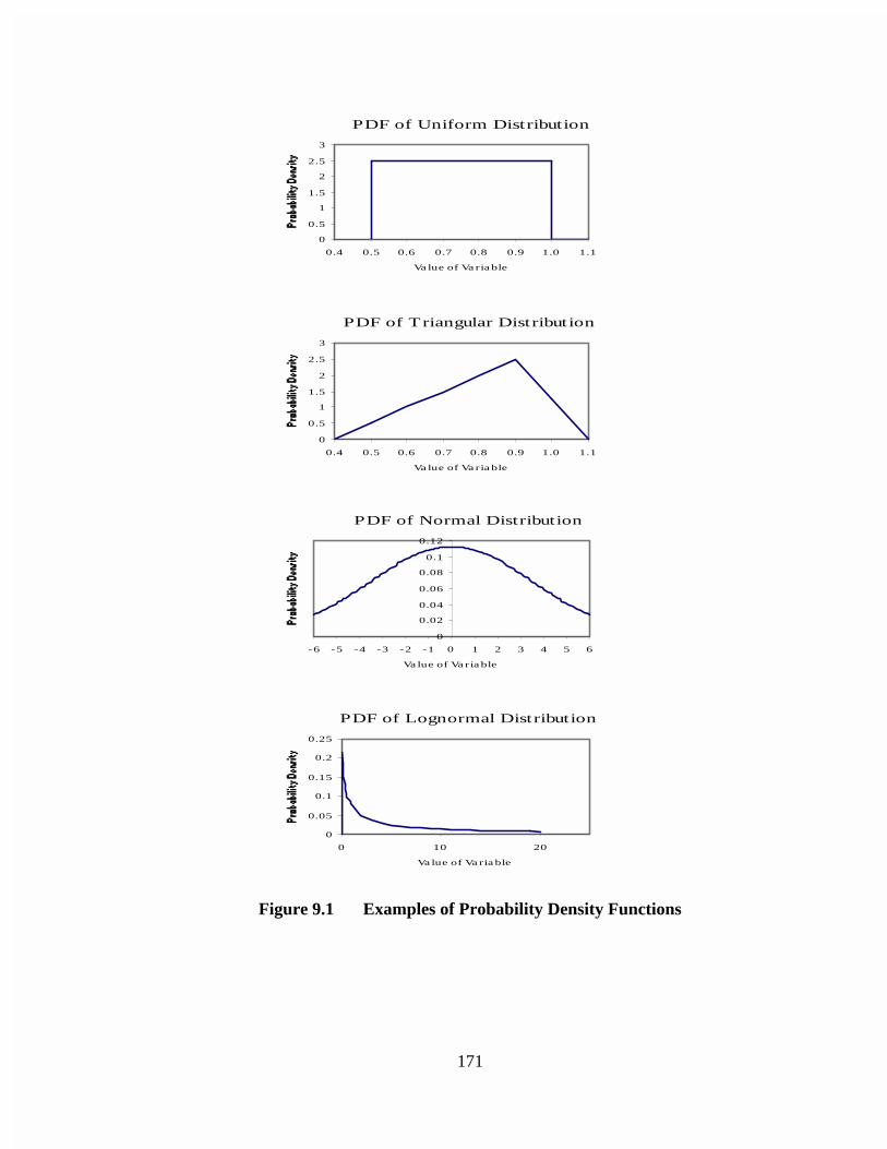
171
PDF of Uniform Distribution
0
0.5
1
1.5
2
2.5
3
0.4 0.5 0.6 0.7 0.8 0.9 1.0 1.1
Value of Variable
PDF of Triangular Distribution
0
0.5
1
1.5
2
2.5
3
0.4 0.5 0.6 0.7 0.8 0.9 1.0 1.1
Value of Variable
PDF of Normal Distribution
0
0.02
0.04
0.06
0.08
0.1
0.12
-6 -5 -4 -3 -2 -1 0 1 2 3 4 5 6
Value of Variable
PDF of Lognormal Distribution
0
0.05
0.1
0.15
0.2
0.25
0 10 20
Value of Variable
Figure 9.1 Examples of Probability Density Functions
172
9.1.4 Monte Carlo Simulation
A probabilistic modeling environment is required to analyze uncertainties in
advanced process technologies. Monte Carlo simulation is one such typical environment
(Ang and Tang, 1984). In this approach, model is run repeatedly, using different values
for each of the uncertain input parameters each time. The values of each of the uncertain
input parameters are generated based on the probability distribution for the parameters. In
each repetition in the simulation, one value for each of the input parameters is sampled
simultaneously. The set of sampled values generated for each of the model output
variables can be analyzed statistically treating them as experimental set of data.
The execution of the model for a given set of samples in a repetition is
deterministic, although the generation of samples values for the input parameters is
probabilistic. However, the Monte Carlo method has the advantage that these
deterministic simulations are repeated in manner that yields important insights into the
sensitivity of the model to variations in the input parameters, as well as into the
likelihood of obtaining any particular outcome.
Monte Carlo methods allow the modeler to use any type of probability
distribution for which values can be generated on a computer, rather than to be restricted
to forms which are analytically tractable. The set of samples obtained for model outputs
can be represented as cumulative distribution functions and summarized using typical
statistics such as mean and variance.
173
In a random Monte Carlo simulation, one approach to generating sample values is
to use the inverse CDF method. A random number generator is used to generate
uniformly distributed numbers between 0 and 1 for each uncertain variable. Thus, the
generated random numbers are used to represent the fractile of the random variable for
which a sample is to be generated. The sample values for the random variables are
calculated using the inverse cumulative distribution functions (CDF's) based on randomly
generated fractiles.
Latin Hypercube Sampling (LHS) is an alternative to random Monte Carlo
simulation. In LHS, the fractiles that are used as inputs to the inverse CDF are not
randomly generated. Instead, the probability distribution for the random variable of
interest is first divided into ranges of equal probability, and one sample is taken from
each equal probability range. However, the order of the samples is random over the
course of simulation, and the pairing of samples between two or more random input
variables is usually treated as independent. In random LHS, one sample is randomly
taken from each equal probability interval, while in median LHS one sample is taken
from the median of the interval (Morgan and Henrion, 1990).
LHS methods guarantee that values from the entire range of distribution will be
sampled proportional to the probability density of the distribution. Thus the input samples
typically cover a full span of each parameter's probability density function compared to
174
when the random Monte Carlo method is used (McKay et al., 1979). The number of
samples required to adequately represent the CDF for a distribution is less for LHS than
for random Monte Carlo sampling. The LHS method was employed in the present study.
9.1.5 Methods for Identifying Key Sources of Uncertainty in Model Inputs
A probabilistic modeling capability has been added to the publicly available
version of ASPEN (Diwekar and Rubin, 1989). A FORTRAN program developed by
Iman and Shortencarier (1984) using LHS was adopted for assigning probability
distributions to model parameters and generating samples from those distributions. In
order to identify the key sources of uncertainty in the model inputs, linear correlations
between the input variables and model outputs can be determined. Linear correlations
between uncertain input variables and the model outputs are identified using techniques
such as standardized regression coefficients (SRC) and partial correlations (PCC). A
FORTAN program which calculates the partial correlation and standardized regression
coefficients was used for analysis of model output (Iman et al., 1985).
The standard regression coefficient of an input variable is used to measure the
relative contribution of the uncertainty in the input variable to the uncertainty of the
output variables. For this analysis, all the sample values for the input variables are
standardized. The standardization process involves subtracting the mean of the variable
from all the sample values and then dividing by the variable's standard deviation. A
multi-variate regression is performed for an output variate based on the inputs. The
175
relative importance of each input variate is indicated by the regression coefficient of that
variate, which is the standardized regression coefficient (SRC). SRCs are the partial
derivatives of the output variable with respect to each input variable. SRCs measure the
shared contribution of the input to the output as all of the simulation input uncertainties
are included in the regression analysis simultaneously.
The partial correlation coefficient analysis is used to identify the degree to which
correlations between output and input random variables may be linear, and it is estimated
in conjunction with multi-variate linear regression analysis using a step-wise procedure.
The input variable most higly correlated with the output variable of interest is assumed as
the starting point for construction of a stepwise linear regression model. In the regression
model, the output variable is treated as a dependent variable and the most highly
correlated input variable is treated as a predictive variable. The PCC technique then
searches for another input variable which is most highly correlated with the residuals of
the regression model already in containing the first input variable. The residual is the
difference between the actual sample value of the dependent variable and the estimated
sample values, using the linear regression model already containing the first input
variable. The process is repeated to add more variables in the analysis. The PCC is a
measure of the unique relationship between input and dependent variables that cannot be
explained by variables already included in the regression analysis (Frey and Rubin,
1992).
176
PCC and SRC analysis is limited to cases where the relationship between input
and output variables is linear. However, these techniques can be extended to monotonic
non-linear cases by performing regressions on the ranks, rather than the sample values of
the inputs and outputs. They are known as partial rank correlation coefficients (PRCC)
and standardized rank regression coefficients (SRCC).
The regression techniques are useful for identifying the contribution of each input
variable to variations in the output variable. However, they cannot be used to identify
which input variables may be responsible for a shift in the central tendency of the model
outputs associated with skewness in the input distributions. In such cases, sensitivity
analysis is performed by gradually making one or more input variables uncertain while
setting point estimates to the remaining input variables and observing the output
distribution. The sensitivity analysis is continued till the current model output distribution
closely resembles the original model output distribution in which all the input variables
are uncertain.
9.2 Input Assumptions for Probabilistic Case Studies
In this section, the base case assumptions regarding uncertainty in specific
performance and cost parameters of the Texaco gasifier-based IGCC system models
developed in the present study are given as listed in Table 9.1, Table 9.2.
177
Tables 9.1 and 9.2 list the performance, environmental, and cost variables selected
for stochastic analysis, along with the deterministic value and distributions for each of
these variables. Since the gas turbine and steam cycle/steam turbine technology is well
established, the performance variables of these process areas were not considered for
uncertainty analysis.
A total of 40 parameters are treated as uncertain in the two cases. These include
assumptions regarding the performance of the gasifier and gas turbine process areas,
capital cost parameters, direct capital costs, maintenance costs, labor rate, and unit costs.
The deterministic values are based upon the assumptions used in published design
studies.
The estimates of uncertainty in the capital cost parameters, including engineering
and home office fees, indirect construction cost factor, and project uncertainty are based
on typical ranges of values for these parameters suggested by EPRI (EPRI, 1986). The
basis for these estimates have been discussed by Frey and Rubin (1991).
The deterministic values for the process contingency factors had been adopted
from assumptions in published design studies (e.g., Frey and Rubin, 1991; Dawkins et
al., 1985). For the purposes of preliminary characterization of uncertainty in capital cost,
it was assumed that the process contingency factors were intended to represent the mid-
point of symmetric uncertainty distributions for process area direct cost. The relative
178
magnitudes of the contingency factors were assumed to suggest the relative magnitude of
the variances to be used. Uniform distributions between the best and worst values were
assumed for some of the process areas, while triangular distribution was assumed for the
other process areas. The triangular distribution was selected in cases where the author felt
that the published contingency factors were carefully developed. The effect of a triangular
distribution, compared to a uniform distribution, is to place more "weight" on the
outcomes near the published contingency factor than on the extreme high or low
outcomes. An exception to the above described approach is the estimate of uncertainty in
the gas turbine process area and is elaborated upon in Frey and Rubin (1991).
The estimates of uncertainty in maintenance cost factors use deterministic values
from published design studies as starting points, similar to the estimates of uncertainty in
direct costs. However, it is assumed that the maintenance costs are more likely to increase
than decrease compared to the deterministic values. This assumption is based on the fact
that IGCC systems must handle material streams containing various contaminants derived
from coal conversion. These contaminants are likely to cause deposition, erosion, and
corrosion problems in various parts of the systems and increase maintenance (Frey and
Rubin, 1991).
The development of estimates for uncertainties in operating cost parameters
including operating labor rate, units costs for ash disposal and byproduct sales, and
byproduct marketing costs factor is similar as discussed in Frey and Rubin (1991).
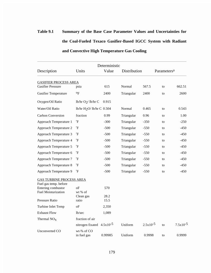
179
Table 9.1 Summary of the Base Case Parameter Values and Uncertainties for
the Coal-Fueled Texaco Gasifier-Based IGCC System with Radiant
and Convective High Temperature Gas Cooling
________________________________________________________________________________________________________________________________________________
DeterministicDescription Units Value Distribution Parametersa________________________________________________________________________________________________________________________________________________
GASIFIER PROCESS AREAGasifier Pressure psia 615 Normal 567.5 to 662.51
Gasifier Temperature oF 2400 Triangular 2400 to 2600
Oxygen/Oil Ratio lb/hr O2/ lb/hr C 0.915
Water/Oil Ratio lb/hr H2O/ lb/hr C 0.504 Normal 0.465 to 0.543
Carbon Conversion fraction 0.99 Triangular 0.96 to 1.00
Approach Temperature 1 oF -300 Triangular -350 to -250
Approach Temperature 2 oF -500 Triangular -550 to -450
Approach Temperature 3 oF -500 Triangular -550 to -450
Approach Temperature 4 oF -500 Triangular -550 to -450
Approach Temperature 5 oF -500 Triangular -550 to -450
Approach Temperature 6 oF -500 Triangular -550 to -450
Approach Temperature 7 oF -500 Triangular -550 to -450
Approach Temperature 8 oF -500 Triangular -550 to -450
Approach Temperature 9 oF -500 Triangular -550 to -450
GAS TURBINE PROCESS AREAFuel gas temp. beforeEntering combustor oF 570Fuel Moisturization wt % of
Clean gas 28.2Pressure Ratio ratio 15.5
Turbine Inlet Temp oF 2,350
Exhaust Flow lb/sec 1,089
Thermal NOx fraction of air
nitrogen fixated 4.5x10⁻⁵ Uniform 2.5x10⁻⁵ to 7.5x10⁻⁵
Unconverted CO wt-% of CO in fuel gas 0.99985 Uniform 0.9998 to 0.9999
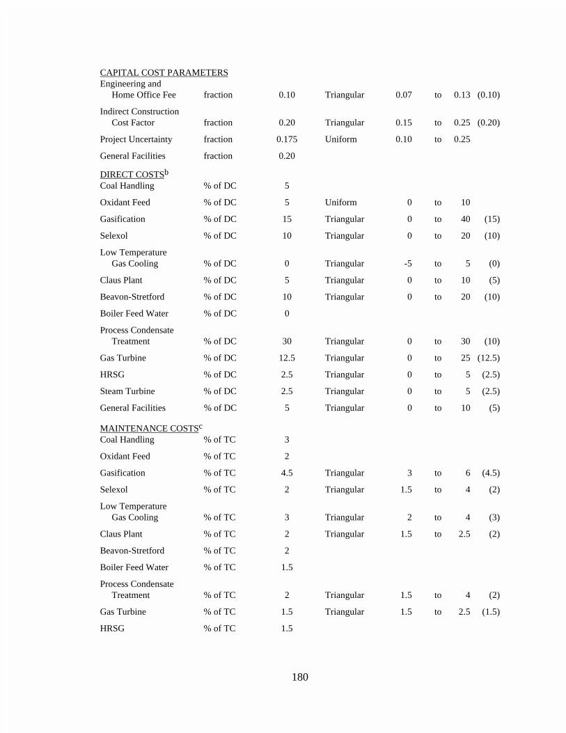
180
CAPITAL COST PARAMETERSEngineering and Home Office Fee fraction 0.10 Triangular 0.07 to 0.13 (0.10)
Indirect Construction Cost Factor fraction 0.20 Triangular 0.15 to 0.25 (0.20)
Project Uncertainty fraction 0.175 Uniform 0.10 to 0.25
General Facilities fraction 0.20
DIRECT COSTSb
Coal Handling % of DC 5
Oxidant Feed % of DC 5 Uniform 0 to 10
Gasification % of DC 15 Triangular 0 to 40 (15)
Selexol % of DC 10 Triangular 0 to 20 (10)
Low Temperature Gas Cooling % of DC 0 Triangular -5 to 5 (0)
Claus Plant % of DC 5 Triangular 0 to 10 (5)
Beavon-Stretford % of DC 10 Triangular 0 to 20 (10)
Boiler Feed Water % of DC 0
Process Condensate Treatment % of DC 30 Triangular 0 to 30 (10)
Gas Turbine % of DC 12.5 Triangular 0 to 25 (12.5)
HRSG % of DC 2.5 Triangular 0 to 5 (2.5)
Steam Turbine % of DC 2.5 Triangular 0 to 5 (2.5)
General Facilities % of DC 5 Triangular 0 to 10 (5)
MAINTENANCE COSTSc
Coal Handling % of TC 3
Oxidant Feed % of TC 2
Gasification % of TC 4.5 Triangular 3 to 6 (4.5)
Selexol % of TC 2 Triangular 1.5 to 4 (2)
Low Temperature Gas Cooling % of TC 3 Triangular 2 to 4 (3)
Claus Plant % of TC 2 Triangular 1.5 to 2.5 (2)
Beavon-Stretford % of TC 2
Boiler Feed Water % of TC 1.5
Process Condensate Treatment % of TC 2 Triangular 1.5 to 4 (2)
Gas Turbine % of TC 1.5 Triangular 1.5 to 2.5 (1.5)
HRSG % of TC 1.5
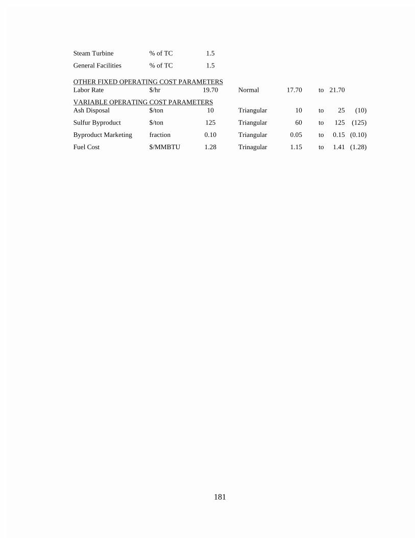
181
Steam Turbine % of TC 1.5
General Facilities % of TC 1.5
OTHER FIXED OPERATING COST PARAMETERSLabor Rate $/hr 19.70 Normal 17.70 to 21.70
VARIABLE OPERATING COST PARAMETERSAsh Disposal $/ton 10 Triangular 10 to 25 (10)
Sulfur Byproduct $/ton 125 Triangular 60 to 125 (125)
Byproduct Marketing fraction 0.10 Triangular 0.05 to 0.15 (0.10)
Fuel Cost $/MMBTU 1.28 Trinagular 1.15 to 1.41 (1.28)
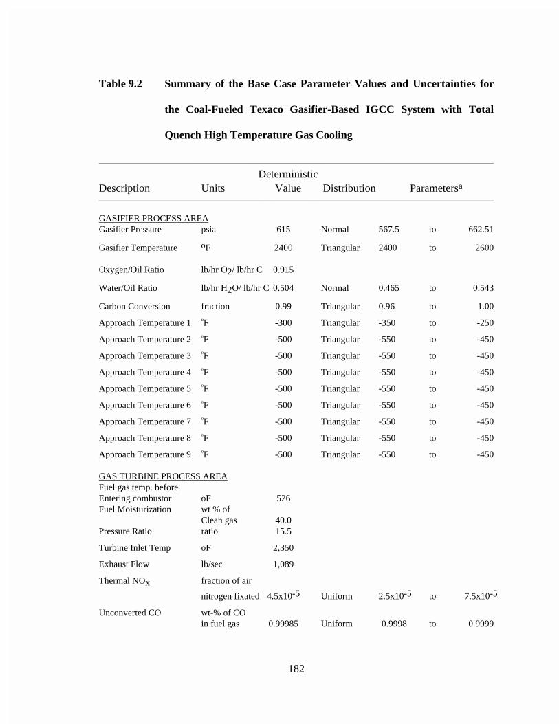
182
Table 9.2 Summary of the Base Case Parameter Values and Uncertainties for
the Coal-Fueled Texaco Gasifier-Based IGCC System with Total
Quench High Temperature Gas Cooling
________________________________________________________________________________________________________________________________________________
DeterministicDescription Units Value Distribution Parametersa________________________________________________________________________________________________________________________________________________
GASIFIER PROCESS AREAGasifier Pressure psia 615 Normal 567.5 to 662.51
Gasifier Temperature oF 2400 Triangular 2400 to 2600
Oxygen/Oil Ratio lb/hr O2/ lb/hr C 0.915
Water/Oil Ratio lb/hr H2O/ lb/hr C 0.504 Normal 0.465 to 0.543
Carbon Conversion fraction 0.99 Triangular 0.96 to 1.00
Approach Temperature 1 oF -300 Triangular -350 to -250
Approach Temperature 2 oF -500 Triangular -550 to -450
Approach Temperature 3 oF -500 Triangular -550 to -450
Approach Temperature 4 oF -500 Triangular -550 to -450
Approach Temperature 5 oF -500 Triangular -550 to -450
Approach Temperature 6 oF -500 Triangular -550 to -450
Approach Temperature 7 oF -500 Triangular -550 to -450
Approach Temperature 8 oF -500 Triangular -550 to -450
Approach Temperature 9 oF -500 Triangular -550 to -450
GAS TURBINE PROCESS AREAFuel gas temp. beforeEntering combustor oF 526Fuel Moisturization wt % of
Clean gas 40.0Pressure Ratio ratio 15.5
Turbine Inlet Temp oF 2,350
Exhaust Flow lb/sec 1,089
Thermal NOx fraction of air
nitrogen fixated 4.5x10⁻⁵ Uniform 2.5x10⁻⁵ to 7.5x10⁻⁵
Unconverted CO wt-% of CO in fuel gas 0.99985 Uniform 0.9998 to 0.9999
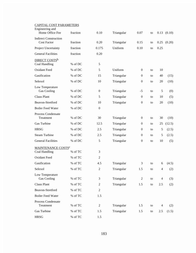
183
CAPITAL COST PARAMETERSEngineering and Home Office Fee fraction 0.10 Triangular 0.07 to 0.13 (0.10)
Indirect Construction Cost Factor fraction 0.20 Triangular 0.15 to 0.25 (0.20)
Project Uncertainty fraction 0.175 Uniform 0.10 to 0.25
General Facilities fraction 0.20
DIRECT COSTSb
Coal Handling % of DC 5
Oxidant Feed % of DC 5 Uniform 0 to 10
Gasification % of DC 15 Triangular 0 to 40 (15)
Selexol % of DC 10 Triangular 0 to 20 (10)
Low Temperature Gas Cooling % of DC 0 Triangular -5 to 5 (0)
Claus Plant % of DC 5 Triangular 0 to 10 (5)
Beavon-Stretford % of DC 10 Triangular 0 to 20 (10)
Boiler Feed Water % of DC 0
Process Condensate Treatment % of DC 30 Triangular 0 to 30 (10)
Gas Turbine % of DC 12.5 Triangular 0 to 25 (12.5)
HRSG % of DC 2.5 Triangular 0 to 5 (2.5)
Steam Turbine % of DC 2.5 Triangular 0 to 5 (2.5)
General Facilities % of DC 5 Triangular 0 to 10 (5)
MAINTENANCE COSTSc
Coal Handling % of TC 3
Oxidant Feed % of TC 2
Gasification % of TC 4.5 Triangular 3 to 6 (4.5)
Selexol % of TC 2 Triangular 1.5 to 4 (2)
Low Temperature Gas Cooling % of TC 3 Triangular 2 to 4 (3)
Claus Plant % of TC 2 Triangular 1.5 to 2.5 (2)
Beavon-Stretford % of TC 2
Boiler Feed Water % of TC 1.5
Process Condensate Treatment % of TC 2 Triangular 1.5 to 4 (2)
Gas Turbine % of TC 1.5 Triangular 1.5 to 2.5 (1.5)
HRSG % of TC 1.5

184
Steam Turbine % of TC 1.5
General Facilities % of TC 1.5
OTHER FIXED OPERATING COST PARAMETERSLabor Rate $/hr 19.70 Normal 17.70 to 21.70
VARIABLE OPERATING COST PARAMETERSAsh Disposal $/ton 10 Triangular 10 to 25 (10)
Sulfur Byproduct $/ton 125 Triangular 60 to 125 (125)
Byproduct Marketing fraction 0.10 Triangular 0.05 to 0.15 (0.10)
Fuel Cost $/MMBTU 1.28 Trinagular 1.15 to 1.41 (1.28)
185
9.3 Probabilistic Analysis of the IGCC Model
For the probabilistic simulation, the deterministic performance, emissions, and
cost model is executed a number of times using LHS, with a different set of values
(samples) assigned to uncertain input parameters each time. The number of times the
deterministic model is executed is equal to the number of observations or sample size
selected. The sample size should be large enough to give sufficient precision to the
numerical simulation as dictated by the use of the model results and at the same time
ensure that the computational time and disk space usage are not excessive (Morgan and
Henrion, 1990). To characterize the mean and the variance of the results and to identify
key uncertainties, a sample size of 100 or greater is typically sufficient (Frey and Rubin,
1991). For the present study, a sample size of 120 was chosen. Results for all the
uncertain output variables are collected at the end of each deterministic run, which can
then be analyzed statistically to gain insight into the key uncertainties of the system. Such
an analysis enables the identification of the key model uncertainties of the most important
determinants of uncertainty in model outputs.
The results of the simulation can be summarized using statistics, such as mean
and standard deviation, or using graphs of the cumulative distribution function and is
discussed in Section 9.5.
The key uncertain variables contributing to the uncertainties in IGCC process
performance were identified using three general approaches. Statistical analysis using
186
regression techniques was used to identify input random variables which are most highly
correlated with uncertainties in output variables. Probabilistic sensitivity analysis was
used for identifying key uncertain inputs. In this approach, the interaction between the
cost and performance uncertain input variables as they affect uncertainty in output
variables can be studied by isolating the uncertainties. For example, one can assign
distributions to one or more input variables while all other model inputs are assigned
point estimates. The third approach, uncertainty screening, which is similar to
probabilistic sensitivity analysis, can be used to confirm the results of a regression or
probabilistic sensitivity analysis by deleting uncertainties from the model inputs which
are not believed to be important and assigning them point estimates. The results of the
screening study can be compared to the results obtained from the original probabilistic
analysis and used to confirm that the deleted uncertainties do not affect the model output
distributions.
A total of six case studies were performed for each technology to characterize the
uncertainty in model outputs and to identify the model inputs that contributed most
significantly to the distribution of values in the model outputs. The general procedure is
illustrated here for the case of radiant and convective-based model. A similar procedure
will be used for the two technologies evaluated. The discussions of the results for all the
three technologies are presented in later sections. The purpose here is to to give a general
description of the approach. The input assumptions for these case studies for the radiant
and convective model are summarized in Table 9.3. Each case study is briefly described:
187
Case 1. Uncertainties were assigned to performance and cost inputs as described
in Table 9.1 and summarized in Table 9.3. This case study has the largest number of
uncertain model inputs of all the case studies.
Case 2. Uncertainties were assigned only to performance input variables as
identified in Table 9.3. The results of this case study, when compared with Case 1, enable
evaluation of the relative contribution of uncertainty in plant performance assumptions to
the overall uncertainty in plant costs.
Case 3. Uncertainties were assigned only to cost input variables as identified in
Table 9.3. The results of this case study, when compared with Case 1, enable evaluation
of the relative contribution of uncertainty in cost assumptions to the overall uncertainty in
plant costs.
Case 4. Only those uncertainties identified as key sources of uncertainty from a
regression analysis of the results of Case 1 were assigned probability distributions, while
all other model inputs were assigned point estimates. In the regression analysis of the
results of Case 1, the model input variables having the highest correlation coefficients
(greater than 0.5) with most of model outputs were selected as the key sources of
uncertainty.
188
Case 5. Only those uncertainties identified as key sources of uncertainty from a
regression analysis of the results of Case 2 were assigned probability distributions, while
all other model inputs were assigned point estimates. In the regression analysis of the
results of Case 2, the model input variables having the highest correlation coefficients
(greater than 0.5) with most of model outputs were selected as the key sources of
uncertainty.
Case 6. Only those uncertainties identified as key sources of uncertainty from a
regression analysis of the results of Case 2 were assigned probability distributions, while
all other model inputs were assigned point estimates. In the regression analysis of the
results of Case 3, the model input variables having the highest correlation coefficients
(greater than 0.5) with most of model outputs were selected as the key sources of
uncertainty.
Tables 9.4 summarizes the above mentioned case studies for total quench coal
model.
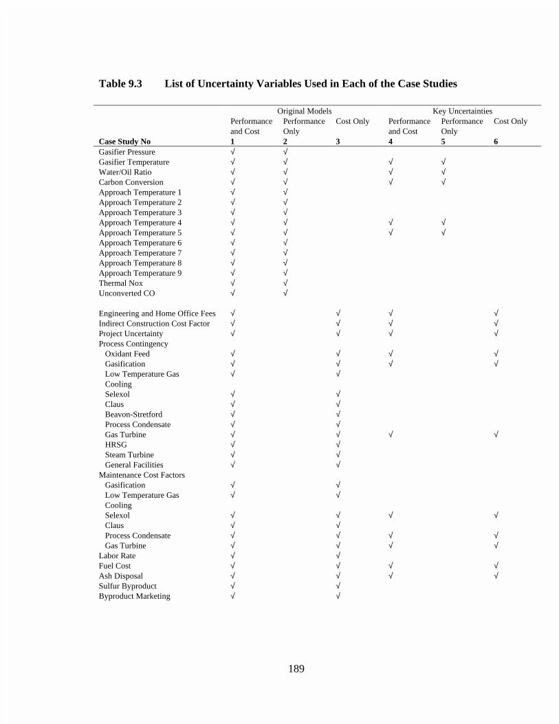
189
Table 9.3 List of Uncertainty Variables Used in Each of the Case Studies
Original Models Key UncertaintiesPerformanceand Cost
PerformanceOnly
Cost Only Performanceand Cost
PerformanceOnly
Cost Only
Case Study No 1 2 3 4 5 6Gasifier Pressure √ √Gasifier Temperature √ √ √ √Water/Oil Ratio √ √ √ √Carbon Conversion √ √ √ √Approach Temperature 1 √ √Approach Temperature 2 √ √Approach Temperature 3 √ √Approach Temperature 4 √ √ √ √Approach Temperature 5 √ √ √ √Approach Temperature 6 √ √Approach Temperature 7 √ √Approach Temperature 8 √ √Approach Temperature 9 √ √Thermal Nox √ √Unconverted CO √ √
Engineering and Home Office Fees √ √ √ √Indirect Construction Cost Factor √ √ √ √Project Uncertainty √ √ √ √Process Contingency Oxidant Feed √ √ √ √ Gasification √ √ √ √ Low Temperature Gas Cooling
√ √
Selexol √ √ Claus √ √ Beavon-Stretford √ √ Process Condensate √ √ Gas Turbine √ √ √ √ HRSG √ √ Steam Turbine √ √ General Facilities √ √Maintenance Cost Factors Gasification √ √ Low Temperature Gas Cooling
√ √
Selexol √ √ √ √ Claus √ √ Process Condensate √ √ √ √ Gas Turbine √ √ √ √Labor Rate √ √Fuel Cost √ √ √ √Ash Disposal √ √ √ √Sulfur Byproduct √ √Byproduct Marketing √ √

190
Table 9.4 List of Uncertainty Variables Used in Each of the Case Studies
Original Models Key UncertaintiesPerformanceand Cost
PerformanceOnly
Cost Only Performanceand Cost
PerformanceOnly
Cost Only
Case Study No 1 2 3 4 5 6Gasifier Pressure √ √Gasifier Temperature √ √ √ √Water/Oil Ratio √ √ √ √Carbon Conversion √ √ √ √Approach Temperature 1 √ √Approach Temperature 2 √ √Approach Temperature 3 √ √Approach Temperature 4 √ √ √ √Approach Temperature 5 √ √ √ √Approach Temperature 6 √ √Approach Temperature 7 √ √Approach Temperature 8 √ √Approach Temperature 9 √ √Thermal Nox √ √Unconverted CO √ √
Engineering and Home Office Fees √ √ √ √Indirect Construction Cost Factor √ √ √ √Project Uncertainty √ √ √ √Process Contingency Oxidant Feed √ √ √ √ Gasification √ √ √ √ Low Temperature Gas Cooling
√ √
Selexol √ √ Claus √ √ Beavon-Stretford √ √ Process Condensate √ √ Gas Turbine √ √ √ √ HRSG √ √ Steam Turbine √ √ General Facilities √ √Maintenance Cost Factors Gasification √ √ Low Temperature Gas Cooling
√ √
Selexol √ √ √ Claus √ √ Process Condensate √ √ √ Gas Turbine √ √ √Labor Rate √ √Fuel Cost √ √ √ √Ash Disposal √ √ √Sulfur Byproduct √ √Byproduct Marketing √ √

191
9.4 Model Results and Applications
Two IGCC systems are evaluated using probabilistic engineering models. All the
systems are Texaco gasifer-based and include: (1) a case of coal-fueled system with
radiant and convective high temperature cooling; and (2) a case of coal-fueled system
with total quench high temperature cooling.
The IGCC system performance models are implemented in the ASPEN chemical
process simulation modeling environment on a DEC VAX Station 3200 mini-computer
using the public version of ASPEN with the stochastic modeling capability. The
simulation process involves several steps. The performance model in ASPEN's keyword-
based input language is read by the ASPEN package and converted to a FORTRAN
program. This first step is called "input translation" and takes approximately 1 to 2
minutes. The ASPEN-generated FORTRAN program is compiled and linked, which also
takes 1 to 2 minutes. The linked ASPEN flowsheet is executed. The final step in the
simulation involves the writing of a report file containing the results of the simulation.
The report writing step may take several minutes depending upon the amount of
information requested by the user regarding the simulation. A single deterministic run
takes a total time of about 5 to 6 minutes. In a stochastic run, the input translation,
compilation and linking takes about 5 minutes and is done only once. The execution of
the compiled program for 120 iterations and report writing takes about 100 minutes.
192
As part of the probabilistic modeling capability in the ASPEN simulator, four
alternative approaches to regression analysis are available for analyzing model results.
The outputs can be analyzed by partial correlation coefficients (PCC), standardized
regression coefficients (SCC), partial rank correlation coefficients (PRCC), and
standardized rank regression coefficients (SRCC).When running stochastic simulation in
ASPEN, the user may specify which type of output analysis is desired. PRCC is the
approach chosen to analyze the case studies.
Cases 1,2, and 3 are run in ASPEN and the distributions for the all outputs are
obtained. The PRCC obtained in each case are analyzed and formed the basis for cases
4,5, and 6 respectively. The outputs which had a PRCC greater than 0.5 or less than –0.5
are identified as key uncertain variables. The PRCCs for the outputs are listed in
Appendix C. The Cases 4, 5, and 6 are run in ASPEN using only the key uncertain
variables identified. It is desired that the cdf’s of the output variables obtained after the
running Cases 4, 5, and 6 are identical to the cdf’s obtained from the results of Cases 1, 2,
and 3 respectively. However, the distributions of the uncertainties in the costs of
electricity and total capital requirement in Cases 1 and 4 were not similar due to the
skewness of some assumptions regarding the unit costs of consumables, some process
contingency factors ,and some maintenance cost factors. This skewness results in a shift
in the central value of the uncertainty in the cost of electricity when uncertainties in
performance and costs are considered. To avoid this shift in the central value of the
uncertainty in the cost of electricity, probabilistic sensitivity analysis was performed by
193
introducing each of the unit cost assumptions, process contingency factors, and
maintenance cost factors one by one as a key uncertainty factor. After introducing one
variable as an uncertain parameter, the model was run again and the distributions were
examined. This procedure was continued till the distributions of the cost of electricity of
Cases 1 and 4 are similar.
Tables 9.5, and 9.6 list the distributions of selected outputs obtained from
executing Case 1 for radiant and convective model and total quench coal model
respectively.
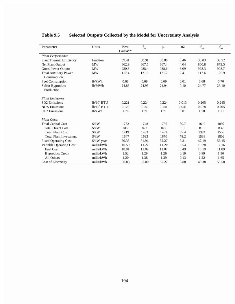
194
Table 9.5 Selected Outputs Collected by the Model for Uncertainty Analysis
Parameter Units BestGuess"”
f.50 µ σ2 f.05 f.95
Plant PerformancePlant Thermal Efficiency Fraction 39.41 38.91 38.88 0.46 38.03 39.52Net Plant Output MW 862.9 867.5 867.4 4.04 860.8 873.5Gross Power Output MW 980.3 988.4 988.6 6.09 978.3 998.7Total Auxiliary Power Consumption
MW 117.4 121.0 121.2 2.41 117.6 125.9
Fuel Consumption lb/kWh 0.68 0.69 0.69 0.01 0.68 0.70Sulfur Byproduct Production
lb/MWh 24.88 24.95 24.94 0.10 24.77 25.10
Plant EmissionsSO2 Emissions lb/106 BTU 0.221 0.224 0.224 0.013 0.205 0.245NOX Emissions lb/106 BTU 0.129 0.140 0.141 0.041 0.078 0.205CO2 Emissions lb/kWh 1.70 1.71 1.71 0.01 1.70 1.71
Plant CostsTotal Capital Cost $/kW 1732 1748 1756 80.7 1619 1892 Total Direct Cost $/kW 815 822 822 5.1 815 832 Total Plant Cost $/kW 1419 1433 1439 67.4 1324 1553 Total Plant Investment $/kW 1647 1663 1670 78.2 1536 1802Fixed Operating Cost $/kW-year 50.35 51.94 52.27 3.31 47.19 58.15Variable Operating Cost mills/kWh 10.59 11.27 11.20 0.54 10.28 12.16 Fuel Cost mills/kWh 10.91 11.09 11.07 0.49 10.19 11.89 Byproduct Credit mills/kWh 1.52 1.29 1.26 0.19 0.89 1.50 All Others mills/kWh 1.20 1.38 1.39 0.13 1.22 1.65Cost of Electricity mills/kWh 50.88 52.00 52.27 3.88 49.38 55.58
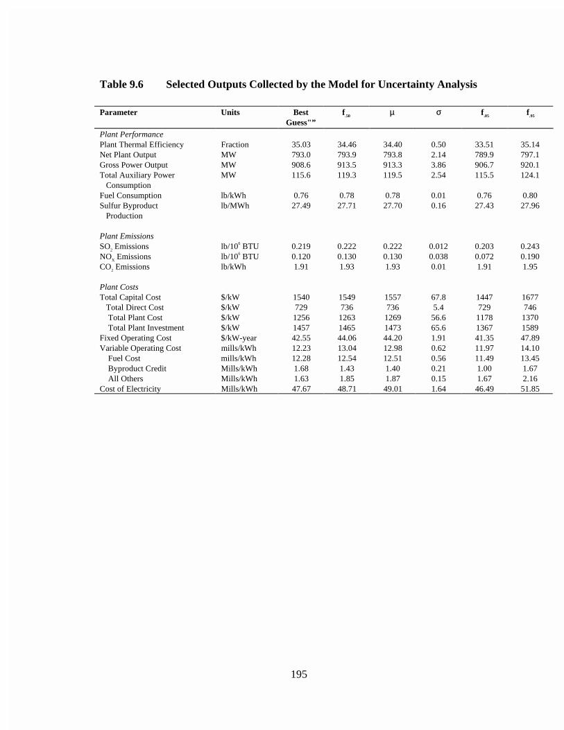
195
Table 9.6 Selected Outputs Collected by the Model for Uncertainty Analysis
Parameter Units BestGuess"”
f.50 µ σ f.05 f.95
Plant PerformancePlant Thermal Efficiency Fraction 35.03 34.46 34.40 0.50 33.51 35.14Net Plant Output MW 793.0 793.9 793.8 2.14 789.9 797.1Gross Power Output MW 908.6 913.5 913.3 3.86 906.7 920.1Total Auxiliary Power Consumption
MW 115.6 119.3 119.5 2.54 115.5 124.1
Fuel Consumption lb/kWh 0.76 0.78 0.78 0.01 0.76 0.80Sulfur Byproduct Production
lb/MWh 27.49 27.71 27.70 0.16 27.43 27.96
Plant EmissionsSO2 Emissions lb/106 BTU 0.219 0.222 0.222 0.012 0.203 0.243NOX Emissions lb/106 BTU 0.120 0.130 0.130 0.038 0.072 0.190CO2 Emissions lb/kWh 1.91 1.93 1.93 0.01 1.91 1.95
Plant CostsTotal Capital Cost $/kW 1540 1549 1557 67.8 1447 1677 Total Direct Cost $/kW 729 736 736 5.4 729 746 Total Plant Cost $/kW 1256 1263 1269 56.6 1178 1370 Total Plant Investment $/kW 1457 1465 1473 65.6 1367 1589Fixed Operating Cost $/kW-year 42.55 44.06 44.20 1.91 41.35 47.89Variable Operating Cost mills/kWh 12.23 13.04 12.98 0.62 11.97 14.10 Fuel Cost mills/kWh 12.28 12.54 12.51 0.56 11.49 13.45 Byproduct Credit Mills/kWh 1.68 1.43 1.40 0.21 1.00 1.67 All Others Mills/kWh 1.63 1.85 1.87 0.15 1.67 2.16Cost of Electricity Mills/kWh 47.67 48.71 49.01 1.64 46.49 51.85
196
The distributions for three important model outputs - total capital cost, levelized
cost of electricity, and plant thermal efficiency are discussed in Section 9.5.
The regression analysis of results of Cases 1, 2 and 3 for the two models indicated
that three performance parameters were significantly correlated with uncertainty in plant
efficiency including carbon conversion, water to feedstock ratio, and gasifier temperature.
For both the total capital cost and levelized cost of electricity, uncertainty in project cost
contingency, engineering and home office fees, indirect construction costs, process
contingency for gas turbine, and fuel cost were found to be influential from the analysis
of Cases 1,2 and 3 for all the three models.
9.5 Analysis of Results
The performance and cost models of the the two models were run using the set of
assumptions regarding uncertainties in process performance and costs shown in Tables
9.3 and 9.4. A deterministic simulation of each of the models was also run which is based
on “best guess” values for the values for the parameters, which are treated as uncertain in
the probabilistic simulation. The deterministic simulation is intended to be representative
of the estimates for plant performance and cost that would be obtained in lieu of
probabilistic simulation, frequency distributions for variables calculated in the
performance and cost models can be estimated. The plant thermal efficiency, the total
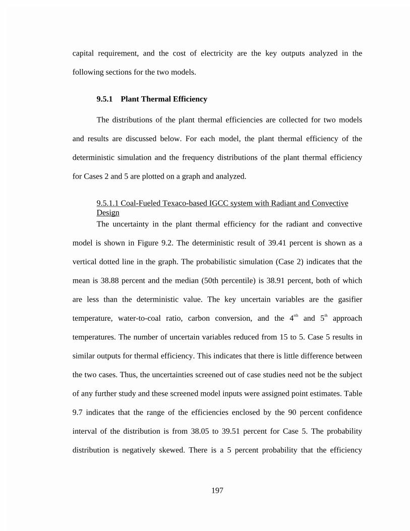
197
capital requirement, and the cost of electricity are the key outputs analyzed in the
following sections for the two models.
9.5.1 Plant Thermal Efficiency
The distributions of the plant thermal efficiencies are collected for two models
and results are discussed below. For each model, the plant thermal efficiency of the
deterministic simulation and the frequency distributions of the plant thermal efficiency
for Cases 2 and 5 are plotted on a graph and analyzed.
9.5.1.1 Coal-Fueled Texaco-based IGCC system with Radiant and ConvectiveDesign
The uncertainty in the plant thermal efficiency for the radiant and convective
model is shown in Figure 9.2. The deterministic result of 39.41 percent is shown as a
vertical dotted line in the graph. The probabilistic simulation (Case 2) indicates that the
mean is 38.88 percent and the median (50th percentile) is 38.91 percent, both of which
are less than the deterministic value. The key uncertain variables are the gasifier
temperature, water-to-coal ratio, carbon conversion, and the 4rth and 5th approach
temperatures. The number of uncertain variables reduced from 15 to 5. Case 5 results in
similar outputs for thermal efficiency. This indicates that there is little difference between
the two cases. Thus, the uncertainties screened out of case studies need not be the subject
of any further study and these screened model inputs were assigned point estimates. Table
9.7 indicates that the range of the efficiencies enclosed by the 90 percent confidence
interval of the distribution is from 38.05 to 39.51 percent for Case 5. The probability
distribution is negatively skewed. There is a 5 percent probability that the efficiency
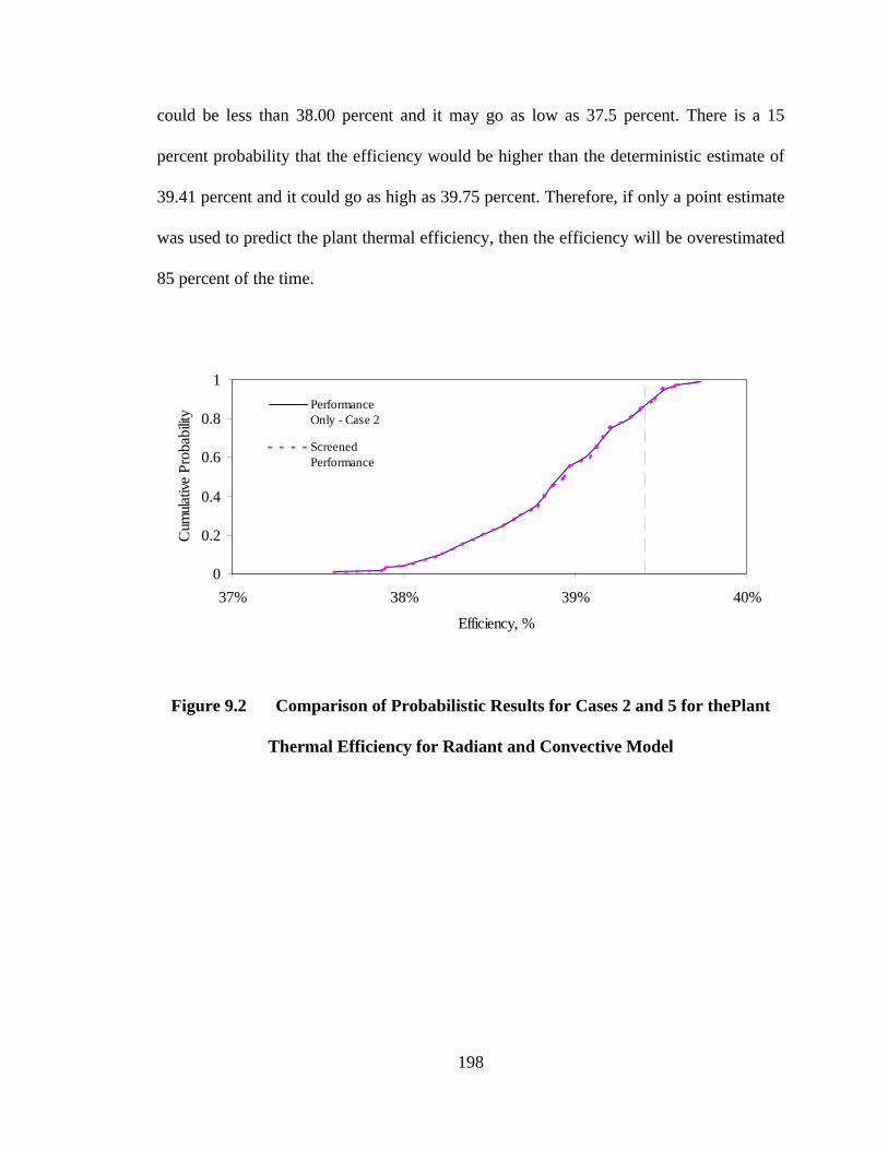
198
could be less than 38.00 percent and it may go as low as 37.5 percent. There is a 15
percent probability that the efficiency would be higher than the deterministic estimate of
39.41 percent and it could go as high as 39.75 percent. Therefore, if only a point estimate
was used to predict the plant thermal efficiency, then the efficiency will be overestimated
85 percent of the time.
0
0.2
0.4
0.6
0.8
1
37% 38% 39% 40%
Efficiency, %
Cum
ulat
ive
Pro
babi
lity
PerformanceOnly - Case 2
ScreenedPerformance
Figure 9.2 Comparison of Probabilistic Results for Cases 2 and 5 for thePlant
Thermal Efficiency for Radiant and Convective Model
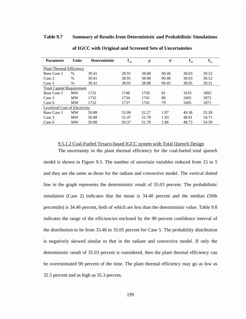
199
Table 9.7 Summary of Results from Deterministic and Probabilistic Simulations
of IGCC with Original and Screened Sets of Uncertainties
Parameter Units Deterministic f.50 µ σ f.05 f.95
Plant Thermal EfficiencyBase Case 1 % 39.41 38.91 38.88 00.46 38.03 39.52Case 2 % 39.41 38.91 38.88 00.46 38.03 39.52Case 5 % 39.41 38.91 38.88 00.45 38.05 39.51Total Capital RequirementBase Case 1 MW 1732 1748 1756 81 1619 1892Case 3 MW 1732 1734 1741 80 1605 1872Case 6 MW 1732 1737 1741 79 1605 1871Levelized Cost of ElectricityBase Case 1 MW 50.88 52.00 52.27 1.97 49.38 55.58Case 3 MW 50.88 51.47 51.78 1.93 48.81 54.71Case 6 MW 50.88 50.37 51.78 1.86 48.73 54.58
9.5.1.2 Coal-Fueled Texaco-based IGCC system with Total Quench Design
The uncertainty in the plant thermal efficiency for the coal-fueled total quench
model is shown in Figure 9.3. The number of uncertain variables reduced from 15 to 5
and they are the same as those for the radiant and convective model. The vertical dotted
line in the graph represents the deterministic result of 35.03 percent. The probabilistic
simulation (Case 2) indicates that the mean is 34.40 percent and the median (50th
percentile) is 34.46 percent, both of which are less than the deterministic value. Table 9.8
indicates the range of the efficiencies enclosed by the 90 percent confidence interval of
the distribution to be from 33.46 to 35.05 percent for Case 5. The probability distribution
is negatively skewed similar to that in the radiant and convective model. If only the
deterministic result of 35.03 percent is considered, then the plant thermal efficiency can
be overestimated 90 percent of the time. The plant thermal efficiency may go as low as
32.5 percent and as high as 35.3 percent.
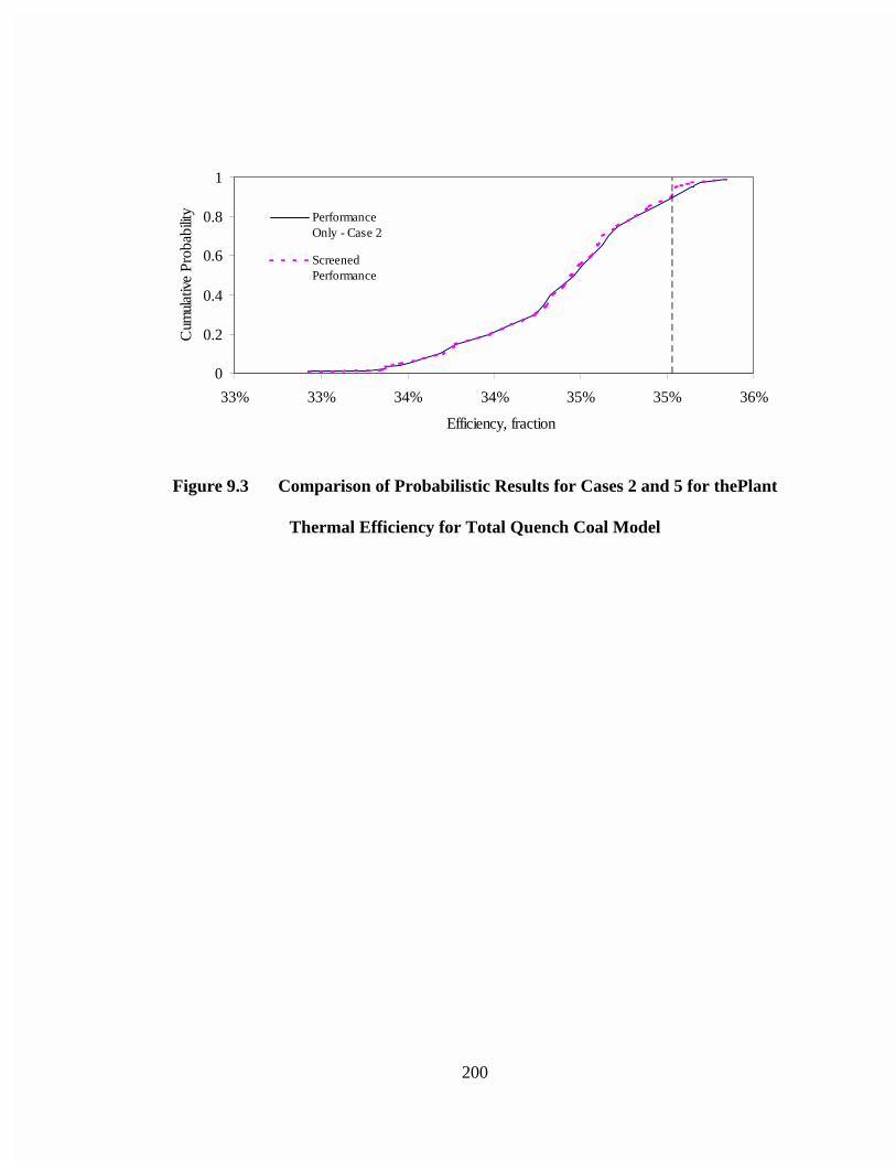
200
0
0.2
0.4
0.6
0.8
1
33% 33% 34% 34% 35% 35% 36%
Efficiency, fraction
Cum
ulat
ive
Pro
babi
lity Performance
Only - Case 2
ScreenedPerformance
Figure 9.3 Comparison of Probabilistic Results for Cases 2 and 5 for thePlant
Thermal Efficiency for Total Quench Coal Model
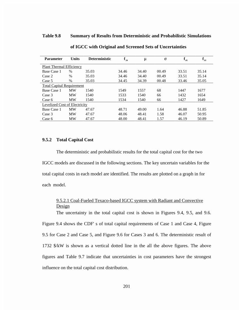
201
Table 9.8 Summary of Results from Deterministic and Probabilistic Simulations
of IGCC with Original and Screened Sets of Uncertainties
Parameter Units Deterministic f.50 µ σ f.05 f.95
Plant Thermal EfficiencyBase Case 1 % 35.03 34.46 34.40 00.49 33.51 35.14Case 2 % 35.03 34.46 34.40 00.49 33.51 35.14Case 5 % 35.03 34.45 34.39 00.48 33.46 35.05Total Capital RequirementBase Case 1 MW 1540 1549 1557 68 1447 1677Case 3 MW 1540 1533 1540 66 1432 1654Case 6 MW 1540 1534 1540 66 1427 1649Levelized Cost of ElectricityBase Case 1 MW 47.67 48.71 49.00 1.64 46.88 51.85Case 3 MW 47.67 48.06 48.41 1.58 46.07 50.95Case 6 MW 47.67 48.00 48.41 1.57 46.19 50.89
9.5.2 Total Capital Cost
The deterministic and probabilistic results for the total capital cost for the two
IGCC models are discussed in the following sections. The key uncertain variables for the
total capital costs in each model are identified. The results are plotted on a graph in for
each model.
9.5.2.1 Coal-Fueled Texaco-based IGCC system with Radiant and ConvectiveDesign
The uncertainty in the total capital cost is shown in Figures 9.4, 9.5, and 9.6.
Figure 9.4 shows the CDF' s of total capital requirements of Case 1 and Case 4, Figure
9.5 for Case 2 and Case 5, and Figure 9.6 for Cases 3 and 6. The deterministic result of
1732 $/kW is shown as a vertical dotted line in the all the above figures. The above
figures and Table 9.7 indicate that uncertainties in cost parameters have the strongest
influence on the total capital cost distribution.
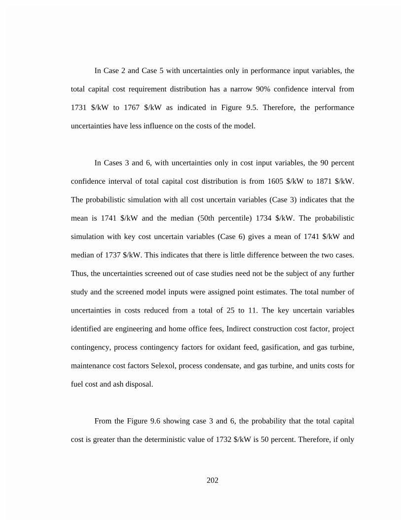
202
In Case 2 and Case 5 with uncertainties only in performance input variables, the
total capital cost requirement distribution has a narrow 90% confidence interval from
1731 $/kW to 1767 $/kW as indicated in Figure 9.5. Therefore, the performance
uncertainties have less influence on the costs of the model.
In Cases 3 and 6, with uncertainties only in cost input variables, the 90 percent
confidence interval of total capital cost distribution is from 1605 $/kW to 1871 $/kW.
The probabilistic simulation with all cost uncertain variables (Case 3) indicates that the
mean is 1741 $/kW and the median (50th percentile) 1734 $/kW. The probabilistic
simulation with key cost uncertain variables (Case 6) gives a mean of 1741 $/kW and
median of 1737 $/kW. This indicates that there is little difference between the two cases.
Thus, the uncertainties screened out of case studies need not be the subject of any further
study and the screened model inputs were assigned point estimates. The total number of
uncertainties in costs reduced from a total of 25 to 11. The key uncertain variables
identified are engineering and home office fees, Indirect construction cost factor, project
contingency, process contingency factors for oxidant feed, gasification, and gas turbine,
maintenance cost factors Selexol, process condensate, and gas turbine, and units costs for
fuel cost and ash disposal.
From the Figure 9.6 showing case 3 and 6, the probability that the total capital
cost is greater than the deterministic value of 1732 $/kW is 50 percent. Therefore, if only
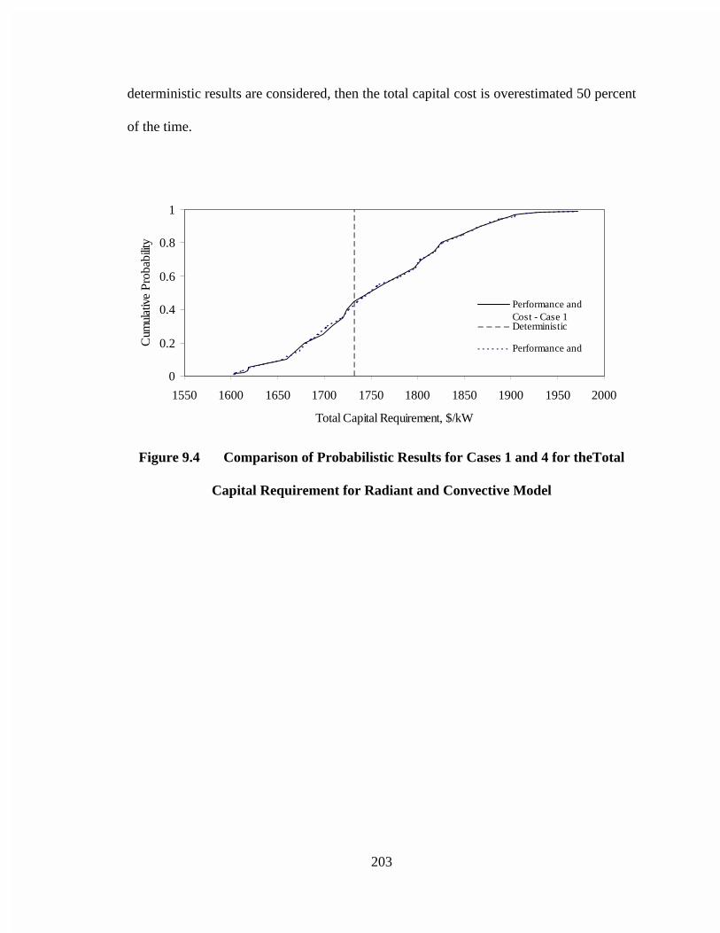
203
deterministic results are considered, then the total capital cost is overestimated 50 percent
of the time.
0
0.2
0.4
0.6
0.8
1
1550 1600 1650 1700 1750 1800 1850 1900 1950 2000
Total Capital Requirement, $/kW
Cum
ulat
ive
Pro
babi
lity
Performance andCost - Case 1Deterministic
Performance and
Figure 9.4 Comparison of Probabilistic Results for Cases 1 and 4 for theTotal
Capital Requirement for Radiant and Convective Model
204
0
0.2
0.4
0.6
0.8
1
1550 1600 1650 1700 1750 1800 1850 1900 1950 2000
Total Capital Requirement, $/kW
Cum
ulat
ive
Prob
abili
ty
Performance Only - Case 2
Deterministic
Performance Key - Case 5
Figure 9.5 Comparison of Probabilistic Results for Cases 2 and 5 for theTotal
Capital Requirement for Radiant and Convective Model
0
0.2
0.4
0.6
0.8
1
1550 1600 1650 1700 1750 1800 1850 1900 1950 2000
Total Capital Requirement, $/kW
Cum
ulat
ive
Prob
abili
ty
Cost Only - Case 3
Deterministic
Cost Only Key - Case 6
Figure 9.6 Comparison of Probabilistic Results for Cases 3 and 6 for theTotal
Capital Requirement for Radiant and Convective Model
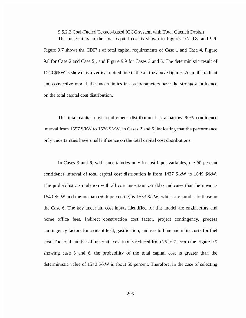
205
9.5.2.2 Coal-Fueled Texaco-based IGCC system with Total Quench Design
The uncertainty in the total capital cost is shown in Figures 9.7 9.8, and 9.9.
Figure 9.7 shows the CDF' s of total capital requirements of Case 1 and Case 4, Figure
9.8 for Case 2 and Case 5 , and Figure 9.9 for Cases 3 and 6. The deterministic result of
1540 $/kW is shown as a vertical dotted line in the all the above figures. As in the radiant
and convective model. the uncertainties in cost parameters have the strongest influence
on the total capital cost distribution.
The total capital cost requirement distribution has a narrow 90% confidence
interval from 1557 $/kW to 1576 $/kW, in Cases 2 and 5, indicating that the performance
only uncertainties have small influence on the total capital cost distributions.
In Cases 3 and 6, with uncertainties only in cost input variables, the 90 percent
confidence interval of total capital cost distribution is from 1427 $/kW to 1649 $/kW.
The probabilistic simulation with all cost uncertain variables indicates that the mean is
1540 $/kW and the median (50th percentile) is 1533 $/kW, which are similar to those in
the Case 6. The key uncertain cost inputs identified for this model are engineering and
home office fees, Indirect construction cost factor, project contingency, process
contingency factors for oxidant feed, gasification, and gas turbine and units costs for fuel
cost. The total number of uncertain cost inputs reduced from 25 to 7. From the Figure 9.9
showing case 3 and 6, the probability of the total capital cost is greater than the
deterministic value of 1540 $/kW is about 50 percent. Therefore, in the case of selecting
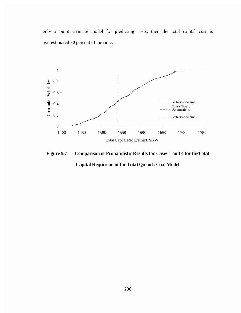
206
only a point estimate model for predicting costs, then the total capital cost is
overestimated 50 percent of the time.
0
0.2
0.4
0.6
0.8
1
1400 1450 1500 1550 1600 1650 1700 1750
Total Capital Requirement, $/kW
Cum
ulat
ive
Pro
babi
lity
Performance andCost - Case 1Deterministic
Performance and
Figure 9.7 Comparison of Probabilistic Results for Cases 1 and 4 for theTotal
Capital Requirement for Total Quench Coal Model
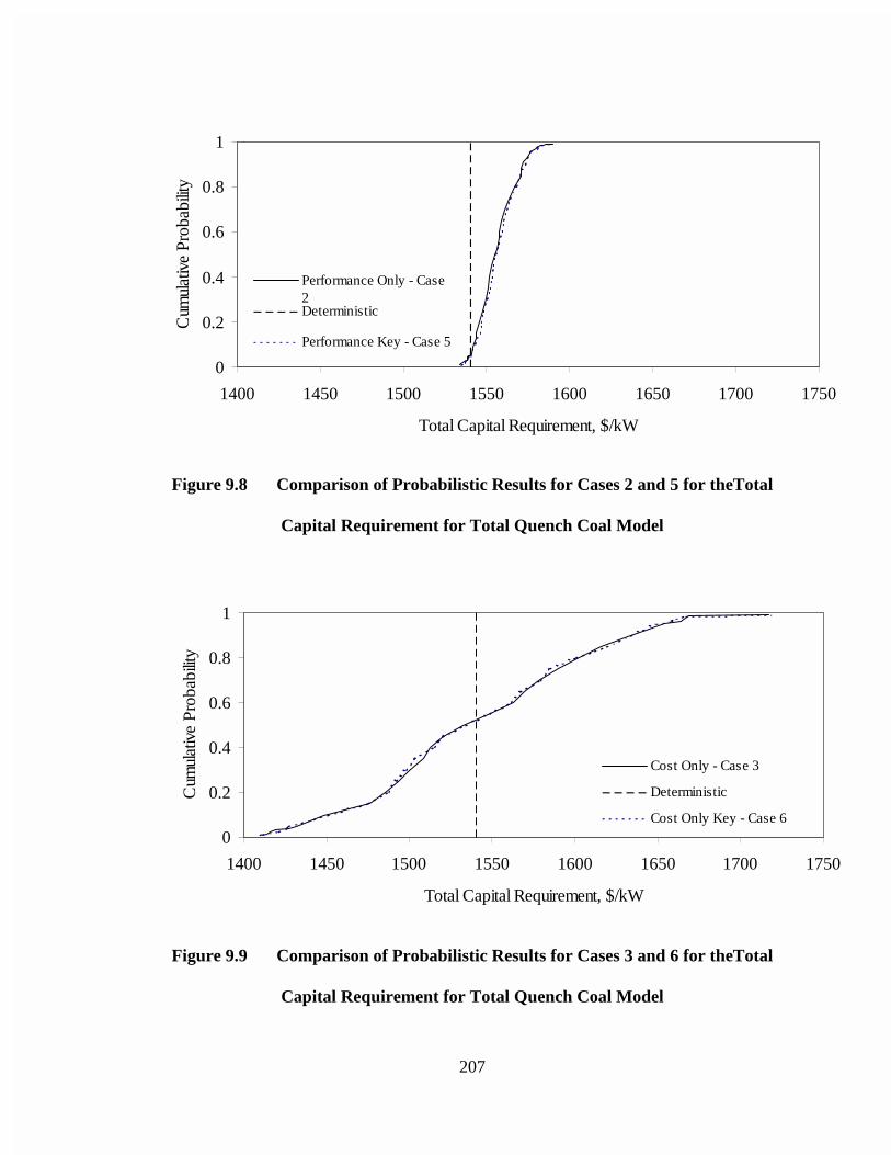
207
0
0.2
0.4
0.6
0.8
1
1400 1450 1500 1550 1600 1650 1700 1750
Total Capital Requirement, $/kW
Cum
ulat
ive
Prob
abili
ty
Performance Only - Case2Deterministic
Performance Key - Case 5
Figure 9.8 Comparison of Probabilistic Results for Cases 2 and 5 for theTotal
Capital Requirement for Total Quench Coal Model
0
0.2
0.4
0.6
0.8
1
1400 1450 1500 1550 1600 1650 1700 1750
Total Capital Requirement, $/kW
Cum
ulat
ive
Prob
abili
ty
Cost Only - Case 3
Deterministic
Cost Only Key - Case 6
Figure 9.9 Comparison of Probabilistic Results for Cases 3 and 6 for theTotal
Capital Requirement for Total Quench Coal Model
208
9.5.3 Cost of Electricity
The following sections discuss the results of probabilistic simulations for the two
IGCC models for the cost of electricity. The deterministic results are analyzed with
respect to the probabilistic results for each model. In the two models, the uncertainties in
cost parameters have the dominating influence on the cost of electricity. Therefore, Cases
3 and 6, which contain uncertainties in only cost inputs, are discussed in detail. The key
uncertainties in cost parameters influencing the cost of electricity are the same as those
described for the total capital cost in each IGCC model.
9.5.3.1 Coal-Fueled Texaco-based IGCC system with Radiant and ConvectiveDesign
The uncertainty in the levelized cost of electricity is shown in Figures 9.10, 9.11,
and 9.12. Figure 9.10 shows the CDF' s of cost of electricity of Case 1 and Case 4, Figure
9.11 for Case 2 and Case 5 , and Figure 9.12 for Cases 3 and 6. The deterministic result
of 50.88 mills/kWh is shown as a vertical dotted line in the all the above figures.
In Cases 3 and 6, with uncertainties only in cost input variables, the 90 percent
confidence interval of cost of electricity distribution is from 48.73 mills/kWh to 54.58
mills/kWh. The probabilistic simulation with all cost uncertain variables (Case 3)
indicates that the mean is 51.78 mills/kWh and the median (50th percentile) 51.47
mills/kWh both of which are higher than that of the deterministic simulation of 51.88
mills/kWh. From the Figure 9.12 showing Case 3 and 6, the total capital cost is
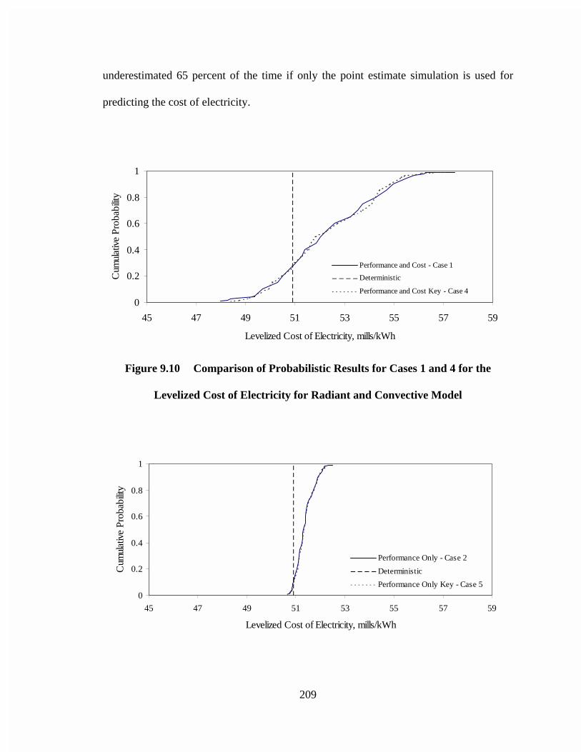
209
underestimated 65 percent of the time if only the point estimate simulation is used for
predicting the cost of electricity.
0
0.2
0.4
0.6
0.8
1
45 47 49 51 53 55 57 59
Levelized Cost of Electricity, mills/kWh
Cum
ulat
ive
Pro
babi
lity
Performance and Cost - Case 1
Deterministic
Performance and Cost Key - Case 4
Figure 9.10 Comparison of Probabilistic Results for Cases 1 and 4 for the
Levelized Cost of Electricity for Radiant and Convective Model
0
0.2
0.4
0.6
0.8
1
45 47 49 51 53 55 57 59
Levelized Cost of Electricity, mills/kWh
Cum
ulat
ive
Pro
babi
lity
Performance Only - Case 2
Deterministic
Performance Only Key - Case 5
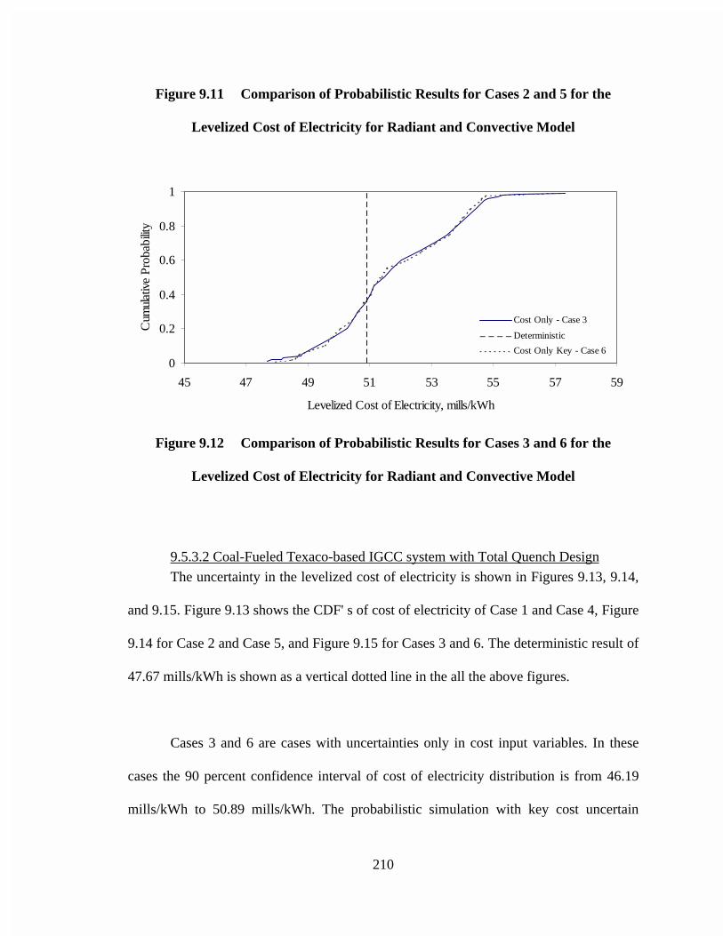
210
Figure 9.11 Comparison of Probabilistic Results for Cases 2 and 5 for the
Levelized Cost of Electricity for Radiant and Convective Model
0
0.2
0.4
0.6
0.8
1
45 47 49 51 53 55 57 59
Levelized Cost of Electricity, mills/kWh
Cum
ulat
ive
Pro
babi
lity
Cost Only - Case 3
Deterministic
Cost Only Key - Case 6
Figure 9.12 Comparison of Probabilistic Results for Cases 3 and 6 for the
Levelized Cost of Electricity for Radiant and Convective Model
9.5.3.2 Coal-Fueled Texaco-based IGCC system with Total Quench Design
The uncertainty in the levelized cost of electricity is shown in Figures 9.13, 9.14,
and 9.15. Figure 9.13 shows the CDF' s of cost of electricity of Case 1 and Case 4, Figure
9.14 for Case 2 and Case 5, and Figure 9.15 for Cases 3 and 6. The deterministic result of
47.67 mills/kWh is shown as a vertical dotted line in the all the above figures.
Cases 3 and 6 are cases with uncertainties only in cost input variables. In these
cases the 90 percent confidence interval of cost of electricity distribution is from 46.19
mills/kWh to 50.89 mills/kWh. The probabilistic simulation with key cost uncertain
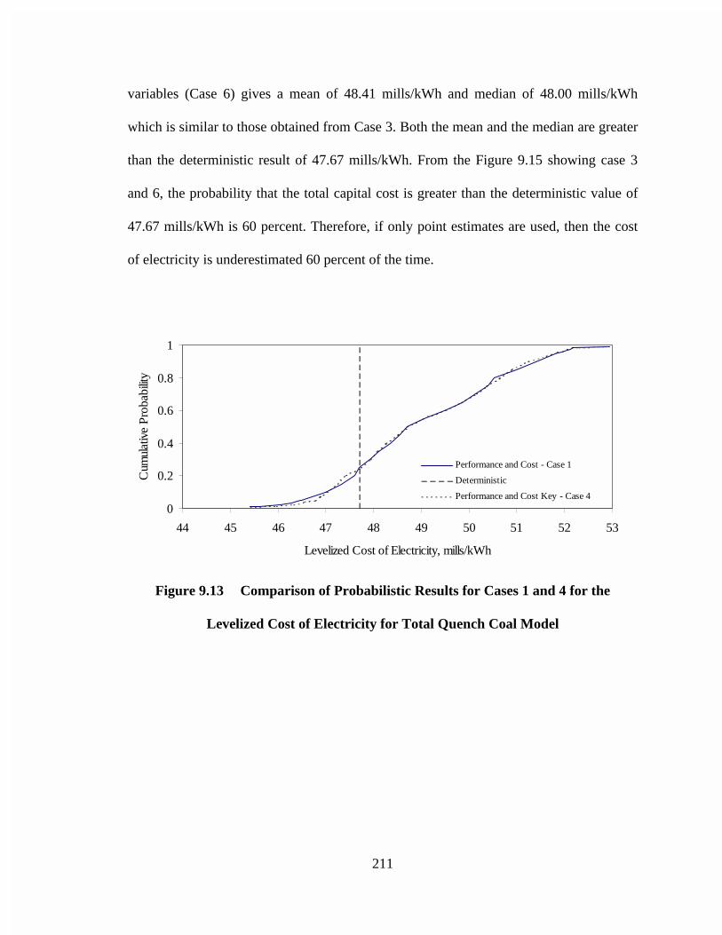
211
variables (Case 6) gives a mean of 48.41 mills/kWh and median of 48.00 mills/kWh
which is similar to those obtained from Case 3. Both the mean and the median are greater
than the deterministic result of 47.67 mills/kWh. From the Figure 9.15 showing case 3
and 6, the probability that the total capital cost is greater than the deterministic value of
47.67 mills/kWh is 60 percent. Therefore, if only point estimates are used, then the cost
of electricity is underestimated 60 percent of the time.
0
0.2
0.4
0.6
0.8
1
44 45 46 47 48 49 50 51 52 53
Levelized Cost of Electricity, mills/kWh
Cum
ulat
ive
Pro
babi
lity
Performance and Cost - Case 1
Deterministic
Performance and Cost Key - Case 4
Figure 9.13 Comparison of Probabilistic Results for Cases 1 and 4 for the
Levelized Cost of Electricity for Total Quench Coal Model
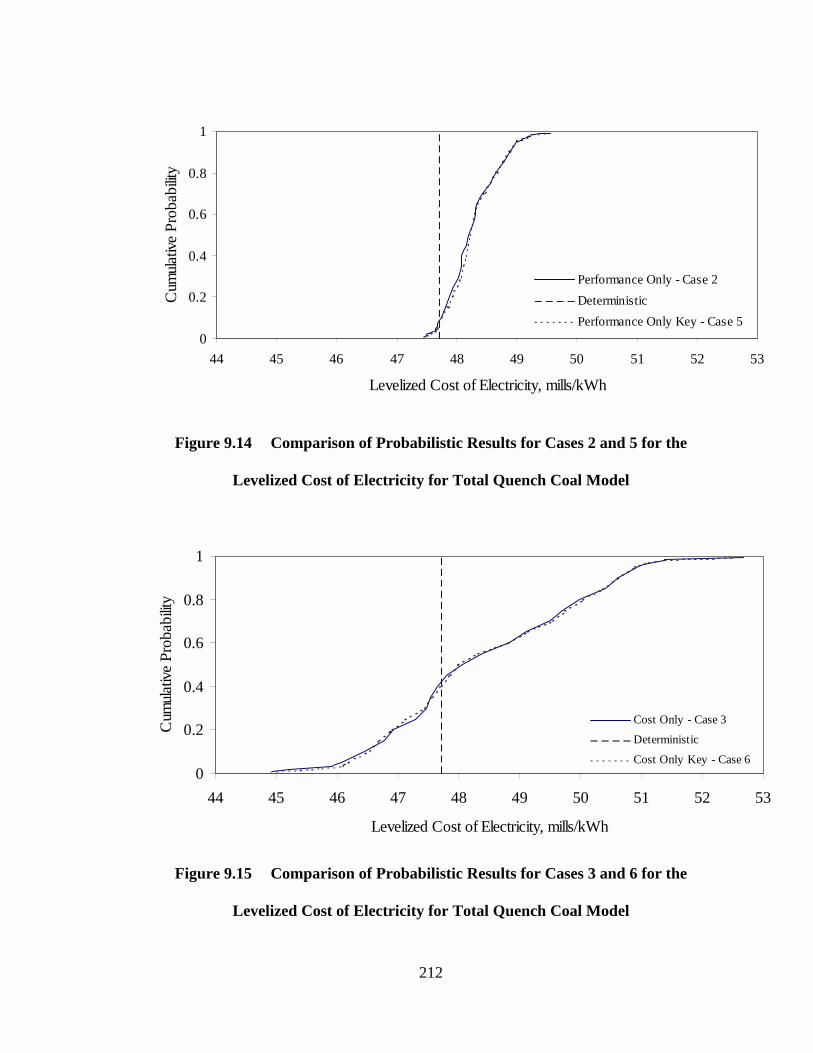
212
0
0.2
0.4
0.6
0.8
1
44 45 46 47 48 49 50 51 52 53
Levelized Cost of Electricity, mills/kWh
Cum
ulat
ive
Prob
abili
ty
Performance Only - Case 2
Deterministic
Performance Only Key - Case 5
Figure 9.14 Comparison of Probabilistic Results for Cases 2 and 5 for the
Levelized Cost of Electricity for Total Quench Coal Model
0
0.2
0.4
0.6
0.8
1
44 45 46 47 48 49 50 51 52 53
Levelized Cost of Electricity, mills/kWh
Cum
ulat
ive
Prob
abili
ty
Cost Only - Case 3
Deterministic
Cost Only Key - Case 6
Figure 9.15 Comparison of Probabilistic Results for Cases 3 and 6 for the
Levelized Cost of Electricity for Total Quench Coal Model
213
9.6 Discussion
The probabilistic analysis indicated that the deterministic case study overestimates
the plant thermal efficiency 85 percent of the time in both the IGCC systems. The
deterministic case study underestimates the cost of electricity 60 to 65 percent of the
time.
The probabilistic analysis indicated that the range of the plant thermal efficiency
of the radiant and convective coal-fueled model (38.0 - 39.5 percent) is higher than that of
the total quench coal-fueled model (33.5 - 35.1 percent). However, the range of cost of
electricity of radiant and convective coal-fueled model (45.4 - 55.6 mills/kWh) and that
of total quench coal-fueled model (46.5 - 51.9 mills/kWh) are similar.
This demonstrates that the plant efficiency of a radiant and convective-based
IGCC system is always higher than that of the coal-fueled total quench-based IGCC
system. However, the cost of electricity of both the coal-fueled systems can be
comparable and further analysis can be done to explore the possibilities of reducing the
costs of the radiant and convective-based system.
214
10.0 CONCLUSIONS
This study documents the development of two Texaco gasifier-based models of
Integrated Gasification Combined Cycle (IGCC) systems: (1) coal-fueled with radiant
and convective high temperature gas cooling; and (2) coal-fueled with total quench high
temperature gas cooling; using ASPEN.
In the first case, a new performance, emissions, and cost model was developed
based upon refinements and modifications to a performance model previously developed
by DOE/FETC. The new model incorporates more performance details regarding key
process areas, such as the gas turbine and gasifier. New comprehensive capital, annual,
and levelized cost models have been developed in this study. In addition, the new model
includes additional features regarding flowsheet calculation sequencing and convergence
schemes, as illustrated by the addition of a number of key design specifications to
enhance the scope of important design assumptions and constraints. The new gas turbine
performance model was calibrated to published data for operation on natural gas and also
to data for operation on syngas. The other IGCC systems developed also contain the
features included for the first model such as the new gas turbine model. The models are
based upon properly sized gas turbines and deal with interactions among all process areas
in order to properly capture differences due to fuel type and gas cooling design thereby
facilitating the comparison of the different models..
215
The models of the Texaco-gasifier based IGCC systems are primarily based on the
findings of a study sponsored by the Electric Power Research Institute (EPRI) (Matchak
et al., 1984). The EPRI study provided extensive process designs which were modified as
deemed appropriate for the development of the current models. The performance model
for radiant and convective high temperature gas cooling design was adopted and modified
from a previous model developed by K.R. Stone in 1985 for Federal Energy Technology
Center (FETC). The performance model for the total quench high temperature gas
cooling model is newly developed in the present study.
Cost models for each of the IGCC system models were developed using
guidelines as suggested by the EPRI Technical Assessment Guide (EPRI, 1986), to
estimate the capital, annual, and levelized costs of the IGCC systems. The cost models
were developed as FORTRAN subroutines which are called by the performance models
of the respective IGCC systems. The inputs to the cost models are provided by the
ASPEN performance models in the form of values for key system variables, such as
flowrates.
An example case study in each of these cases illustrates the type of results that
may be obtained from the model regarding plant performance, emissions, and cost. The
results indicate that of the two IGCC system models using coal as fuel to the gasifier, the
IGCC system using the radiant and convective high temperature gas cooling has a higher
plant efficiency of 39.4 percent, and higher cost of electricity of 50.88 mills/kWh than the
216
IGCC system using the total quench high temperature gas cooling design, which has a
plant efficiency of 35.0 percent and cost of electricity of 47.67 mills/kWh.
The radiant and convective model has higher plant efficiency than that of the total
quench coal-fueled model due to the additional steam generation in the gasifier process
which in turn results in more power generation from the steam turbines. However, the
radiant and convective coolers are expensive units to maintain resulting in higher costs in
the case of the radiant and convective model than those of the total quench coal-fueled
model.
IGCC is in the early stages of development. It has been demonstrated for only
first-of-a-kind applications and there is not much history regarding the performance of
these systems. Therefore, there are inherent uncertainties in the performance and cost
parameter estimates. Therefore incorporation of uncertainties is critical for the design and
evaluation of the IGCC systems.
The efficiency, total capital cost, and cost of electricity of an IGCC system
depends on the values of key design and performance variables and cost parameter
assumptions. The new IGCC systems developed in the present study were applied
extensively in probabilistic case studies to evaluate the response of the models to changes
in these parameters and to identify key uncertainties. The uncertainties in the IGCC
systems were characterized by a systematic approach. In each of the three IGCC systems,
217
a probabilistic model was developed to account for uncertainties in the performance
parameters and cost parameters. The stochastic capability of ASPEN was used to perform
the probabilistic analysis. The results from the probabilistic model simulations included
possible ranges of values for the performance, emissions, and cost variables of the IGCC
system. These results were used to identify the key uncertainties.
The total uncertain input variables initially assumed were 40. The total number of
key uncertainty variables were atmost 16 in any of the three cases. This reduction in the
number of uncertainties reduces the costs of conducting research in the less uncertain
process areas. The key uncertain performance input variables include the gasifier
temperature, the carbon conversion and the water-to-fuel ratio. The uncertainties in these
parameters largely influence the plant thermal efficiency and net plant output. This
indicates that significant research has to be done in the gasifier process area to reduce
risks or poor plant efficiencies. Uncertainties in the engineering and home office fees, the
project contingency, the indirect construction factor, and the fuel cost largely influence
the capital, annual, and levelized cost of all the three IGCC systems.
The probabilistic analysis indicated that the deterministic case study overestimates
the plant thermal efficiency 85 percent of the time in both the IGCC systems. The
deterministic case study underestimates the cost of electricity 60 to 65 percent of the
time.
218
The probabilistic analysis indicated that the range of the plant thermal efficiency
of the radiant and convective coal-fueled model (38.0 - 39.5 percent) is higher than that of
the total quench coal-fueled model (33.5 - 35.1 percent). However, the range of cost of
electricity of radiant and convective coal-fueled model (45.4 - 55.6 mills/kWh) and that
of total quench coal-fueled model (46.5 - 51.9 mills/kWh) are similar.
This demonstrates that the plant efficiency of a radiant and convective-based
IGCC system is always higher than that of the coal-fueled total quench-based IGCC
system. However, the cost of electricity of both the coal-fueled systems can be
comparable and further analysis can be done to explore the possibilities of reducing the
costs of the radiant and convective-based system.
The radiant and convective model has high costs compared to conventional power
plants. However, it might be competitive in terms of high plant efficiencies and low
emissions. The coal-fueled total quench model has higher costs and lower plant
efficiencies than the conventional power plants. Therefore, it may not have any
competitive edge in the United States except under stringent NOX and SO2 regulations.
The probabilistic analysis can be used to identify key process areas which have
potential for further research, to possibly optimally configure the IGCC systems, and also
to compare more comprehensively the trade-offs between the three technologies. The
uncertainties in the costs can be reduced by a detailed cost estimate study. The models

219
will be used in future work as a benchmark for comparison with more advanced and
technologically-risky power generation system concepts.
220
11.0 REFERENCES
Agarwal, P, and H.C. Frey (1995), “Development and Application of Performance and
Cost Models for the Externally-Fired Combined Cycle, ” Task 1 Topical Report, Volume
2, DOE/MC/29094--5246-Vol.2, Prepared by North Carolina State University for
Carnegie Mellon University and U.S. Department of Energy, Morgantown, West
Virginia, July.
Agarwal, P. and H.C. Frey (1996), “Modeling and Assessment of the Externally-Fired
Combined Cycle System,” Prepared by North Carolina State University for U.S.
Department of Energy, Morgantown, WV.
Anand, A.K., F.C. Jahnke, and R.R. Olson, Jr (1992), “High Efficiency Quench
Gasification Combined Cycles with Integrated Air Separation,” Proceedings of Eleventh
EPRI Conference on Gasification Power Plants, Electric Power Research Institute, Inc.,
Palo Alto, CA, October.
Bharvirkar, R. and H.C. Frey (1998), “Development of Simplified Performance and Cost
Models of Integrated Gasification Combined Cycle Systems, ” Prepared by North
Carolina State University for Carnegie Mellon University, Pittsburgh, Pennsylvania, July.
221
Bjorge, R and M. Jandrisevits (1996), “IGCC Technology for the 21st Century,” 1996
Gasification Technologies Conference, Electric Power Research Institute, Inc., Palo Alto,
CA, October.
Buchanan, T. L., M.R. DeLallo, and J.S. White (1998), “Economic Evaluation of
Advanced Coal Gasification Technologies for Power Generation,” 1998 Gasification
Technologies Conference, Electric Power Research Institute, Inc., Palo Alto, CA,
October.
DeMoss, T.B. (1995), “Gas, Coal Duke it out Over Repowering,” Power Engineering,
21-24, June.
Doering, E.L., and U. Mahagaokar (1992), “Benefits of Heat Recovery vs Water Quench
in Coal or Petroleum Coke Gasification for Power Generation,” Proceedings of Eleventh
EPRI Conference on Gasification Power Plants, Electric Power Research Institute, Inc.,
Palo Alto, CA, October.
EPRI, (1986), “TAGTM - Technical Assessment Guide, Volume1: Electricity Supply -
1986,” P-4463-SR, Electric Power Research Institute, Inc., Palo Alto, CA, December.
222
Eustis, F. H. and M.S. Johnson (1990), “Gas Turbine Effects on Integrated-Gasification-
Combined-Cycle Power Plant Operations,” GS/ER-6770, Prepared by Stanford
University for Electric Power Research Institute, Inc, Palo Alto, CA, March.
Farina, G.L., L. Bressan, and D. Todd (1998), “IGCC Capital Cost and Performance, ”
1998 Gasification Technologies Conference, Electric Power Research Institute, Inc., San
Francisco, CA, October.
Farmer, R (1997); Gas Turbine World; Pequot Publishing Inc., Fairfield, CT; Vol 18., p
44.
Frey, H.C. and E.S. Rubin (1990), “Stochastic Modeling of Coal Gasification Combined
Cycle Systems: Cost Models for Selected IGCC Systems,” Report No. DOE/MC/24248-
2901 (NTIS No. DE90015345). June. Prepared by Carnegie Mellon University for U.S.
Department of Energy, Morgantown, WV.
Frey, H.C. and E.S. Rubin (1991), “Development and Application of a Probabilistic
Evaluation Method for Advanced Process Technologies,” DOE/MC 24248-3105
(DE91002095), Prepared by Carnegie Mellon University for U.S. Department of Energy,
Morgantown, WV, April.

223
Frey, H.C., and E.S. Rubin (1992a), "Evaluate Uncertainties in Advanced Process
Technologies," Chemical Engineering Process, p 63-70, May.
Frey, H.C., and E.S. Rubin (1992b), "Evaluation of Advanced Coal Gasification
Combined-Cycle Systems under Uncertainty," Ind. Eng. Chem. Res., 31: 1299-1307.
Frey, H.C., and E.S. Rubin (1992c), "Integration of Coal Utilization and Environmental
Control in Integrated Gasification Combined Cycle Systems," Environ. Sci. and Tech.,
26(10):1982-1990.
Frey, H.C. (1994), "Development and Application of Performance and Cost Models for
Gas Turbine-Based Selective Catalytic Reduction NOx Control," Task 1 Topical Report,
Volume 1, Prepared by North Carolina State University for Carnegie Mellon University
and U.S. Department of Energy, Morgantown, West Virginia, October.
Frey, H.C., E. Rubin, and U. Diwekar (1994), "Modeling Uncertainties in Advanced
Technologies: Application to a Coal Gasification System with Hot Gas Cleanup,"
Energy, 19(4):449-463.
224
Frey, H.C., and R.B. Williams (1995), "Performance and Cost Models for the Direct
Sulfur Recovery Process," Task 1 Topical Report, Volume 3, DOE/MC/29094--5246-
Vol.3, Prepared by North Carolina State University for Carnegie Mellon University and
U.S. Department of Energy, Morgantown, West Virginia, September.
Frey, H.C. (1998), "Quantitative Analysis of Variability and Uncertainty in Energy and
Environmental Systems," Chapter 23 in Uncertainty Modeling and Analysis in Civil
Engineering, B. M. Ayyub, ed., CRC Press: Boca Raton, FL.
Hager, R. L., and D. L. Heaven (1990), “Evaluation of a Dow-Based Gasification-
Combined-Cycle Plant Using Bituminous Coal,” GS-6904. Prepared by Flour Daniel, Inc
for EPRI, Irvine, CA
Holt, N. (1998), " IGCC Power Plants - EPRI Design & Cost Studies," Proceedings of
EPRI/GTC Gasification Technologies Conference, Electric Power Research Institute,
Inc., San Francisco, CA, October.
225
Iman, R.L., and M.J. Shortencarier (1984), A FORTRAN 7 Program and User's Guide for
the Generation of Latin Hypercube and Random Samples for Use with Computer Models,
Report No. SAND83-2365, Sandia National Laboratories, Albuquerque, NM. March.
Iman, R.L., and M.J. Shortencarier and J. D. Johnson (1985), A FORTRAN 7 Program
and User's Guide for the Calculation of Partial Correlation and Standardized Regression
Coefficients, Report No. SAND85-0044, Sandia National Laboratories, Albuquerque,
NM. June.
Kerkhof, F.P.J.M. and P.van Steerderen (1993), “Integration of Gas Turbine and Air
Separation Unit for IGCC Power Plants,” Netherlands Agency for Energy and the
Environment, Amsterdam, Netherlands. August.
Matchak, T.A., A.D. Rao, V. Ramanathan et al. (1984), “Cost and Performance for
Commercial Applications of Texaco-Based Gasification-Combined-Cycle Plants,” AP-
3486. Prepared by Flour Engineers, Inc for EPRI, Palo Alto, CA.
Merrow, E. W., Phillips, K. E., Myers, C. W. (1981), "Understanding Cost Growth and
Performance Shortfalls in Pioneer Process Plants," Report No. R-2569-DOE, Rand
Corporation, Santa Monica, CA, September.
226
McNamee, G.P., and G.A. White (1986), “Use of Lignite in Texaco Gasification-Based-
Combined-Cycle Power Plants,” AP-4509. Prepared by Energy Conversion Systems, Inc
for EPRI, Los Angeles, CA.
Mendez-Vigo, I., J. Pisa, J. Cortes et al. (1998), “The Puertollano IGCC plant: Status
Update,” 1998 Gasification Technologies Conference, Electric Power Research Institute,
Inc., Palo Alto, CA, October.
Morgan, M.G., and M. Henrion (1990), Uncertainty: A Guide to Dealing with
Uncertainty in Quantitative Risk and Policy Analysis, Cambridge University Press: New
York.
Nowacki, P. (1981), Coal Gasification Processes, Noyes Data Corporation, Park Ridge,
NJ, p 256.
Pietruszkiewicz, Milkavich, Booras et al. (1988), “An Evaluation of IGCC and PCFS
plants, ” AP-5950. Prepared by Bechtel Group, Inc for EPRI, Palo Alto, CA.
Preston, W.E. (1996), "Texaco Gasification: Powering the 90's," 1996 Gasification
Technologies Conference, Electric Power Research Institute, Inc., Palo Alto, CA,
October.
227
Rocha, M. F., and H.C. Frey (1997), “Cost Modeling of a Texaco Coal Gasification
Combined Cycle System, ” Prepared by North Carolina State University for Carnegie
Mellon University and U.S. Department of Energy, Morgantown, WV, August.
Sendin, U., W.Schellberg, W.Empsperger, et al. (1996), “ The Pertollano IGCC Project,
A 335 MW Demonstration Power Plant for the Electricity Companies in Europe,” 1996
Gasification Technologies Conference, Electric Power Research Institute, Inc., Palo Alto,
CA, October.
Simbeck D. R., R.L. Dickenson, and E.D. Oliver (1983), “Coal Gasification Systems: A
Guide to Status, Applications, and Economics,” AP-3109 Prepared by Synthetic Fuel
Associates, Inc for Electric Power Research Institute, Palo Alto, California.
Simbeck, D. R. and R.L. Dickenson (1996), “The EPRI Coal Gasification Guidebook - A
Review of the Recent Update,” 1996 Gasification Technologies Conference, Electric
Power Research Institute, Inc., Palo Alto, CA, October.
Smith, J., and D. Heaven (1992), “Evaluation of a 510-Mwe Destec GCC Power Plant
Fueled With Illinois No. 6 Coal,” TR-100319. Prepared by Flour Daniel, Inc for EPRI,
Irvine, CA
Supp., E. (1990), How to Produce Methanol from Coal, Springer-Verlag, New York.
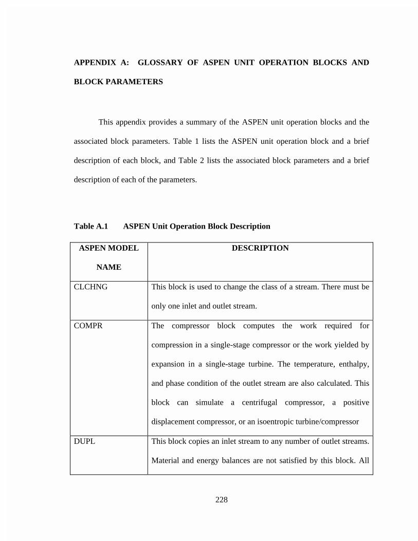
228
APPENDIX A: GLOSSARY OF ASPEN UNIT OPERATION BLOCKS AND
BLOCK PARAMETERS
This appendix provides a summary of the ASPEN unit operation blocks and the
associated block parameters. Table 1 lists the ASPEN unit operation block and a brief
description of each block, and Table 2 lists the associated block parameters and a brief
description of each of the parameters.
Table A.1 ASPEN Unit Operation Block Description
ASPEN MODEL
NAME
DESCRIPTION
CLCHNG This block is used to change the class of a stream. There must be
only one inlet and outlet stream.
COMPR The compressor block computes the work required for
compression in a single-stage compressor or the work yielded by
expansion in a single-stage turbine. The temperature, enthalpy,
and phase condition of the outlet stream are also calculated. This
block can simulate a centrifugal compressor, a positive
displacement compressor, or an isoentropic turbine/compressor
DUPL This block copies an inlet stream to any number of outlet streams.
Material and energy balances are not satisfied by this block. All
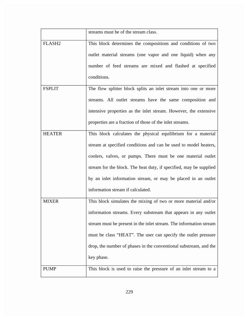
229
streams must be of the stream class.
FLASH2 This block determines the compositions and conditions of two
outlet material streams (one vapor and one liquid) when any
number of feed streams are mixed and flashed at specified
conditions.
FSPLIT The flow splitter block splits an inlet stream into one or more
streams. All outlet streams have the same composition and
intensive properties as the inlet stream. However, the extensive
properties are a fraction of those of the inlet streams.
HEATER This block calculates the physical equilibrium for a material
stream at specified conditions and can be used to model heaters,
coolers, valves, or pumps. There must be one material outlet
stream for the block. The heat duty, if specified, may be supplied
by an inlet information stream, or may be placed in an outlet
information stream if calculated.
MIXER This block simulates the mixing of two or more material and/or
information streams. Every substream that appears in any outlet
stream must be present in the inlet stream. The information stream
must be class “HEAT”. The user can specify the outlet pressure
drop, the number of phases in the conventional substream, and the
key phase.
PUMP This block is used to raise the pressure of an inlet stream to a
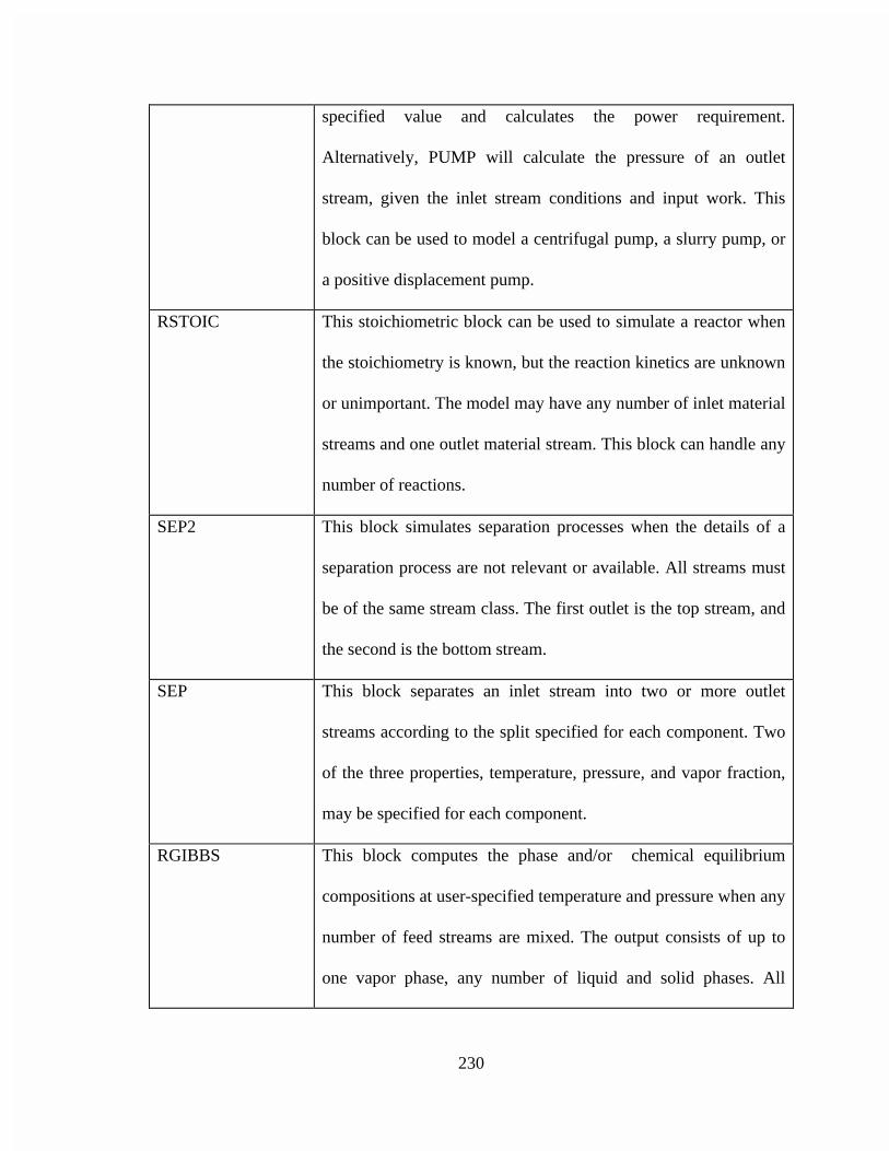
230
specified value and calculates the power requirement.
Alternatively, PUMP will calculate the pressure of an outlet
stream, given the inlet stream conditions and input work. This
block can be used to model a centrifugal pump, a slurry pump, or
a positive displacement pump.
RSTOIC This stoichiometric block can be used to simulate a reactor when
the stoichiometry is known, but the reaction kinetics are unknown
or unimportant. The model may have any number of inlet material
streams and one outlet material stream. This block can handle any
number of reactions.
SEP2 This block simulates separation processes when the details of a
separation process are not relevant or available. All streams must
be of the same stream class. The first outlet is the top stream, and
the second is the bottom stream.
SEP This block separates an inlet stream into two or more outlet
streams according to the split specified for each component. Two
of the three properties, temperature, pressure, and vapor fraction,
may be specified for each component.
RGIBBS This block computes the phase and/or chemical equilibrium
compositions at user-specified temperature and pressure when any
number of feed streams are mixed. The output consists of up to
one vapor phase, any number of liquid and solid phases. All
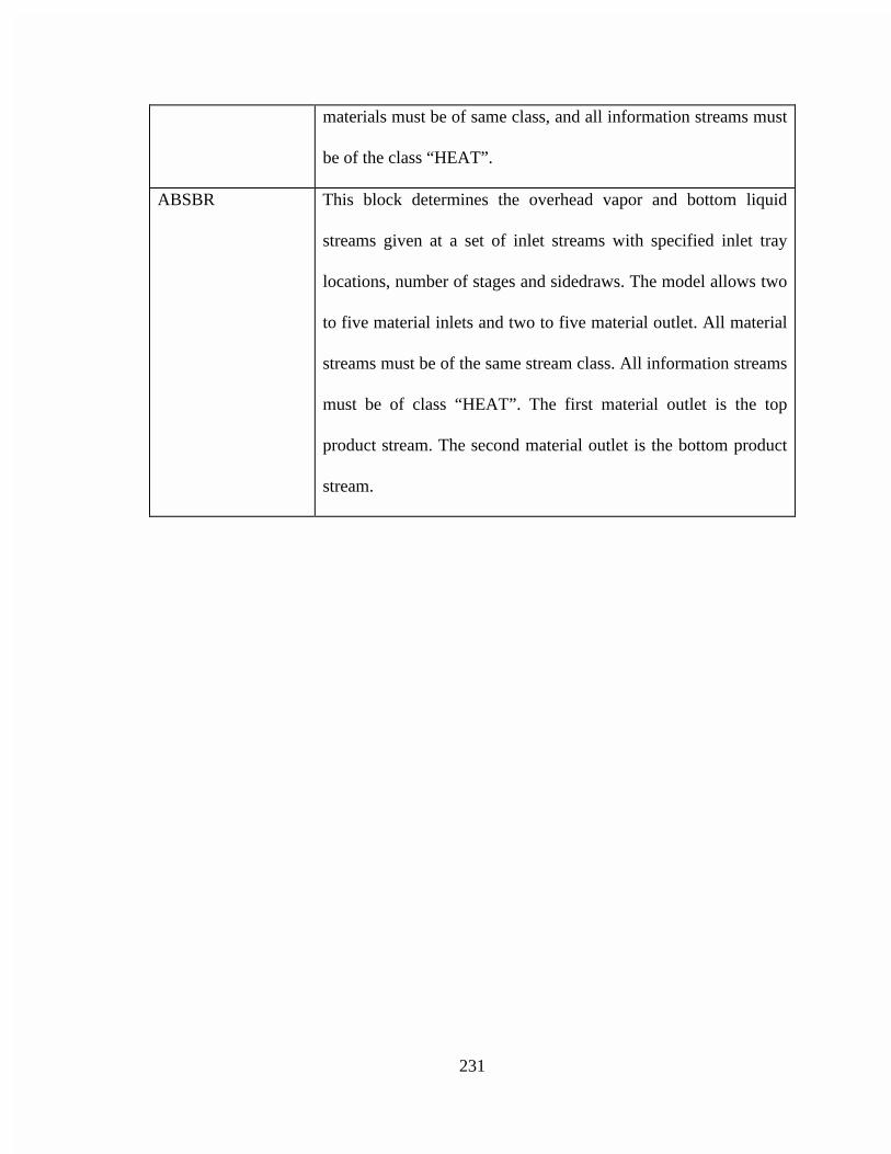
231
materials must be of same class, and all information streams must
be of the class “HEAT”.
ABSBR This block determines the overhead vapor and bottom liquid
streams given at a set of inlet streams with specified inlet tray
locations, number of stages and sidedraws. The model allows two
to five material inlets and two to five material outlet. All material
streams must be of the same stream class. All information streams
must be of class “HEAT”. The first material outlet is the top
product stream. The second material outlet is the bottom product
stream.
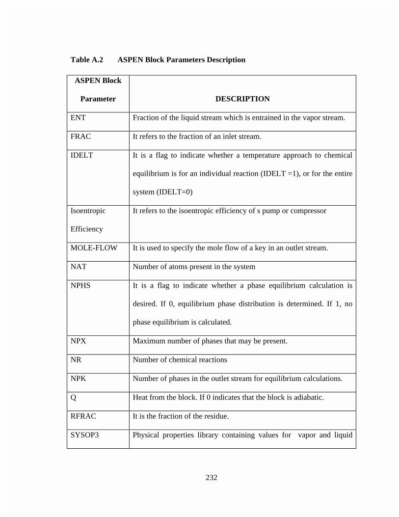
232
Table A.2 ASPEN Block Parameters Description
ASPEN Block
Parameter DESCRIPTION
ENT Fraction of the liquid stream which is entrained in the vapor stream.
FRAC It refers to the fraction of an inlet stream.
IDELT It is a flag to indicate whether a temperature approach to chemical
equilibrium is for an individual reaction (IDELT =1), or for the entire
system (IDELT=0)
Isoentropic
Efficiency
It refers to the isoentropic efficiency of s pump or compressor
MOLE-FLOW It is used to specify the mole flow of a key in an outlet stream.
NAT Number of atoms present in the system
NPHS It is a flag to indicate whether a phase equilibrium calculation is
desired. If 0, equilibrium phase distribution is determined. If 1, no
phase equilibrium is calculated.
NPX Maximum number of phases that may be present.
NR Number of chemical reactions
NPK Number of phases in the outlet stream for equilibrium calculations.
Q Heat from the block. If 0 indicates that the block is adiabatic.
RFRAC It is the fraction of the residue.
SYSOP3 Physical properties library containing values for vapor and liquid
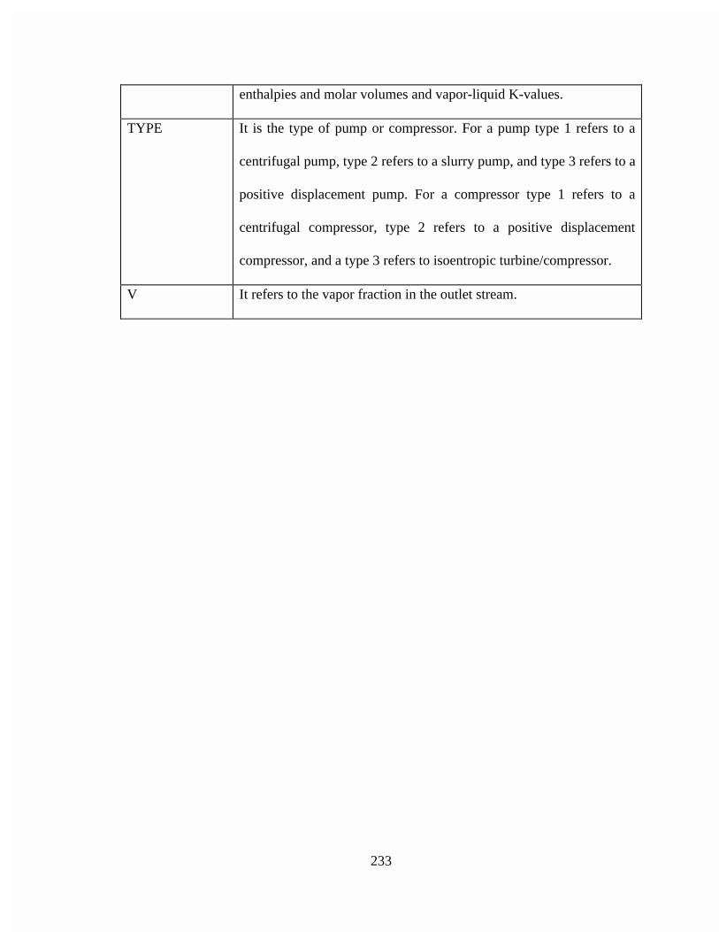
233
enthalpies and molar volumes and vapor-liquid K-values.
TYPE It is the type of pump or compressor. For a pump type 1 refers to a
centrifugal pump, type 2 refers to a slurry pump, and type 3 refers to a
positive displacement pump. For a compressor type 1 refers to a
centrifugal compressor, type 2 refers to a positive displacement
compressor, and a type 3 refers to isoentropic turbine/compressor.
V It refers to the vapor fraction in the outlet stream.
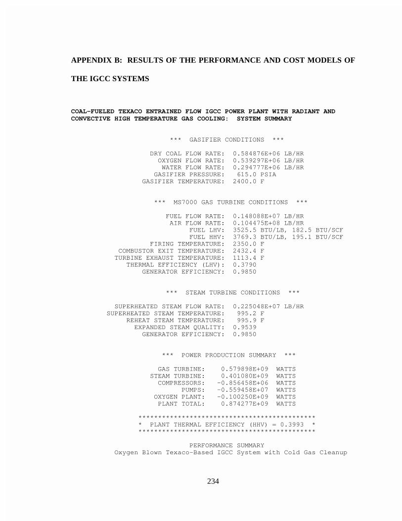
234
APPENDIX B: RESULTS OF THE PERFORMANCE AND COST MODELS OF
THE IGCC SYSTEMS
COAL-FUELED TEXACO ENTRAINED FLOW IGCC POWER PLANT WITH RADIANT ANDCONVECTIVE HIGH TEMPERATURE GAS COOLING: SYSTEM SUMMARY
*** GASIFIER CONDITIONS ***
DRY COAL FLOW RATE: 0.584876E+06 LB/HR OXYGEN FLOW RATE: 0.539297E+06 LB/HR WATER FLOW RATE: 0.294777E+06 LB/HR GASIFIER PRESSURE: 615.0 PSIA GASIFIER TEMPERATURE: 2400.0 F
*** MS7000 GAS TURBINE CONDITIONS ***
FUEL FLOW RATE: 0.148088E+07 LB/HR AIR FLOW RATE: 0.104475E+08 LB/HR FUEL LHV: 3525.5 BTU/LB, 182.5 BTU/SCF FUEL HHV: 3769.3 BTU/LB, 195.1 BTU/SCF FIRING TEMPERATURE: 2350.0 F COMBUSTOR EXIT TEMPERATURE: 2432.4 F TURBINE EXHAUST TEMPERATURE: 1113.4 F THERMAL EFFICIENCY (LHV): 0.3790 GENERATOR EFFICIENCY: 0.9850
*** STEAM TURBINE CONDITIONS ***
SUPERHEATED STEAM FLOW RATE: 0.225048E+07 LB/HR SUPERHEATED STEAM TEMPERATURE: 995.2 F REHEAT STEAM TEMPERATURE: 995.9 F EXPANDED STEAM QUALITY: 0.9539 GENERATOR EFFICIENCY: 0.9850
*** POWER PRODUCTION SUMMARY ***
GAS TURBINE: 0.579898E+09 WATTS STEAM TURBINE: 0.401080E+09 WATTS COMPRESSORS: -0.856458E+06 WATTS PUMPS: -0.559458E+07 WATTS OXYGEN PLANT: -0.100250E+09 WATTS PLANT TOTAL: 0.874277E+09 WATTS
********************************************* * PLANT THERMAL EFFICIENCY (HHV) = 0.3993 * *********************************************
PERFORMANCE SUMMARY Oxygen Blown Texaco-Based IGCC System with Cold Gas Cleanup
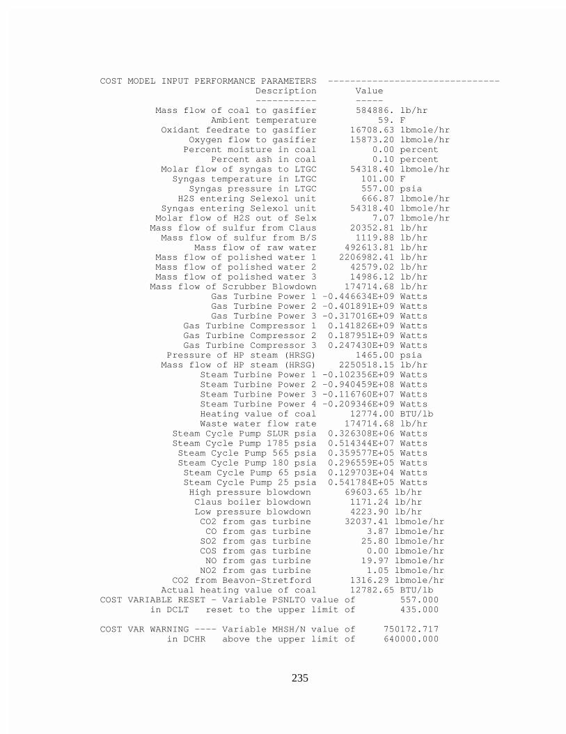
235
COST MODEL INPUT PERFORMANCE PARAMETERS ------------------------------- Description Value ----------- ----- Mass flow of coal to gasifier 584886. lb/hr Ambient temperature 59. F Oxidant feedrate to gasifier 16708.63 lbmole/hr Oxygen flow to gasifier 15873.20 lbmole/hr Percent moisture in coal 0.00 percent Percent ash in coal 0.10 percent Molar flow of syngas to LTGC 54318.40 lbmole/hr Syngas temperature in LTGC 101.00 F Syngas pressure in LTGC 557.00 psia H2S entering Selexol unit 666.87 lbmole/hr Syngas entering Selexol unit 54318.40 lbmole/hr Molar flow of H2S out of Selx 7.07 lbmole/hr Mass flow of sulfur from Claus 20352.81 lb/hr Mass flow of sulfur from B/S 1119.88 lb/hr Mass flow of raw water 492613.81 lb/hr Mass flow of polished water 1 2206982.41 lb/hr Mass flow of polished water 2 42579.02 lb/hr Mass flow of polished water 3 14986.12 lb/hr Mass flow of Scrubber Blowdown 174714.68 lb/hr Gas Turbine Power 1 -0.446634E+09 Watts Gas Turbine Power 2 -0.401891E+09 Watts Gas Turbine Power 3 -0.317016E+09 Watts Gas Turbine Compressor 1 0.141826E+09 Watts Gas Turbine Compressor 2 0.187951E+09 Watts Gas Turbine Compressor 3 0.247430E+09 Watts Pressure of HP steam (HRSG) 1465.00 psia Mass flow of HP steam (HRSG) 2250518.15 lb/hr Steam Turbine Power 1 -0.102356E+09 Watts Steam Turbine Power 2 -0.940459E+08 Watts Steam Turbine Power 3 -0.116760E+07 Watts Steam Turbine Power 4 -0.209346E+09 Watts Heating value of coal 12774.00 BTU/lb Waste water flow rate 174714.68 lb/hr Steam Cycle Pump SLUR psia 0.326308E+06 Watts Steam Cycle Pump 1785 psia 0.514344E+07 Watts Steam Cycle Pump 565 psia 0.359577E+05 Watts Steam Cycle Pump 180 psia 0.296559E+05 Watts Steam Cycle Pump 65 psia 0.129703E+04 Watts Steam Cycle Pump 25 psia 0.541784E+05 Watts High pressure blowdown 69603.65 lb/hr Claus boiler blowdown 1171.24 lb/hr Low pressure blowdown 4223.90 lb/hr CO2 from gas turbine 32037.41 lbmole/hr CO from gas turbine 3.87 lbmole/hr SO2 from gas turbine 25.80 lbmole/hr COS from gas turbine 0.00 lbmole/hr NO from gas turbine 19.97 lbmole/hr NO2 from gas turbine 1.05 lbmole/hr CO2 from Beavon-Stretford 1316.29 lbmole/hr Actual heating value of coal 12782.65 BTU/lbCOST VARIABLE RESET - Variable PSNLTO value of 557.000 in DCLT reset to the upper limit of 435.000
COST VAR WARNING ---- Variable MHSH/N value of 750172.717 in DCHR above the upper limit of 640000.000
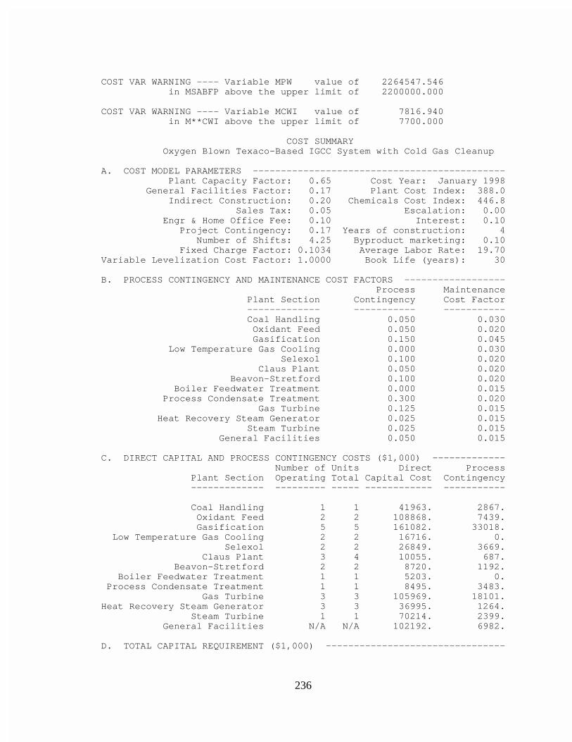
236
COST VAR WARNING ---- Variable MPW value of 2264547.546 in MSABFP above the upper limit of 2200000.000
COST VAR WARNING ---- Variable MCWI value of 7816.940 in M**CWI above the upper limit of 7700.000
COST SUMMARY Oxygen Blown Texaco-Based IGCC System with Cold Gas Cleanup
A. COST MODEL PARAMETERS --------------------------------------------- Plant Capacity Factor: 0.65 Cost Year: January 1998 General Facilities Factor: 0.17 Plant Cost Index: 388.0 Indirect Construction: 0.20 Chemicals Cost Index: 446.8 Sales Tax: 0.05 Escalation: 0.00 Engr & Home Office Fee: 0.10 Interest: 0.10 Project Contingency: 0.17 Years of construction: 4 Number of Shifts: 4.25 Byproduct marketing: 0.10 Fixed Charge Factor: 0.1034 Average Labor Rate: 19.70Variable Levelization Cost Factor: 1.0000 Book Life (years): 30
B. PROCESS CONTINGENCY AND MAINTENANCE COST FACTORS ------------------ Process Maintenance Plant Section Contingency Cost Factor ------------- ----------- ----------- Coal Handling 0.050 0.030 Oxidant Feed 0.050 0.020 Gasification 0.150 0.045 Low Temperature Gas Cooling 0.000 0.030 Selexol 0.100 0.020 Claus Plant 0.050 0.020 Beavon-Stretford 0.100 0.020 Boiler Feedwater Treatment 0.000 0.015 Process Condensate Treatment 0.300 0.020 Gas Turbine 0.125 0.015 Heat Recovery Steam Generator 0.025 0.015 Steam Turbine 0.025 0.015 General Facilities 0.050 0.015
C. DIRECT CAPITAL AND PROCESS CONTINGENCY COSTS ($1,000) ------------- Number of Units Direct Process Plant Section Operating Total Capital Cost Contingency ------------- --------- ----- ------------ -----------
Coal Handling 1 1 41963. 2867. Oxidant Feed 2 2 108868. 7439. Gasification 5 5 161082. 33018. Low Temperature Gas Cooling 2 2 16716. 0. Selexol 2 2 26849. 3669. Claus Plant 3 4 10055. 687. Beavon-Stretford 2 2 8720. 1192. Boiler Feedwater Treatment 1 1 5203. 0. Process Condensate Treatment 1 1 8495. 3483. Gas Turbine 3 3 105969. 18101.Heat Recovery Steam Generator 3 3 36995. 1264. Steam Turbine 1 1 70214. 2399. General Facilities N/A N/A 102192. 6982.
D. TOTAL CAPITAL REQUIREMENT ($1,000) --------------------------------

237
Description Annual Cost ----------- ----------- Total Direct Cost 703322. Indirect Construction Cost 140664. Sales Tax 28836. Engineering and Home Office Fees 87282. Environmental Permitting 1000. Total Indirect Costs 257783. Total Process Contingencies 81100. Project Contingency 182386. Total Plant Cost 1224590. AFDC 196241. Total Plant Investment 1420831. Preproduction (Startup) Costs 34522. Inventory Capital 14564. Initial Catalysts and Chemicals 7366. Land 2745. TOTAL CAPITAL REQUIREMENT ($1,000) --------> 1494237.
E. FIXED OPERATING COSTS ($/year) ------------------------------------ Description Annual Cost ----------- ----------- Operating Labor 7488364. Maintenance Costs 30097578. Administration and Supervision 5858219. TOTAL FIXED OPERATING COST ($/year) --------------> 43444161.
F. VARIABLE OPERATING COSTS ------------------------------------------ 1. CONSUMABLES ($/year) Material Annual Description Unit Cost Requirement Operating Cost ----------- --------- ----------- -------------- Sulfuric Acid: 119.52 $/ton 1539.8 ton/yr 184039. NaOH: 239.04 $/ton 317.7 ton/yr 75933. Na2 HPO4: 0.76 $/lb 1230.7 lb/yr 936. Hydrazine: 3.48 $/lb 5915.3 lb/yr 20567. Morpholine: 1.41 $/lb 5492.2 lb/yr 7758. Lime: 86.92 $/ton 709.7 ton/yr 61689. Soda Ash: 173.85 $/ton 782.5 ton/yr 136032. Corrosion Inh.: 2.06 $/lb 141601.1 lb/yr 292327. Surfactant: 1.36 $/lb 141601.1 lb/yr 192321. Chlorine: 271.64 $/ton 21.7 ton/yr 5886. Biocide: 3.91 $/lb 24053.8 lb/yr 94088. Selexol Solv.: 1.96 $/lb 55557.5 lb/yr 108659. Claus Catalyst: 478.08 $/ton 12.7 ton/yr 6078. Sul.. Acid Cat: 2.06 $/liter 0.0 liter/yr 0. SCOT Catalyst: 249.91 $/ft3 0.0 ft3/yr 0. SCOT Chemicals: 0.39 $/ft3 0.0 ft3/yr 0. B/S Catalyst: 184.71 $/ft3 62.3 ft3/yr 11510. B/S Chemicals: N/A N/A 134457. Fuel Oil: 45.64 $/bbl 48949.5 bbl/yr 2233815. Plant Air Ads.: 3.04 $/lb 3671.2 lb/yr 11169. Raw Water: 0.79 $/Kgal 336233.6 Kgal/yr 266694. Waste Water: 912.70 $/gpm ww 174714.7 lb/hr 207079. LPG - Flare: 12.71 $/bbl 4283.1 bbl/yr 54449. TOTAL CONSUMABLES ($/year) -----------------------> 4105485.
2. FUEL, ASH DISPOSAL, AND BYPRODUCT CREDIT ($/year) Coal: 1.26 $/MMBtu 584885.7 lb/hr 53619480.
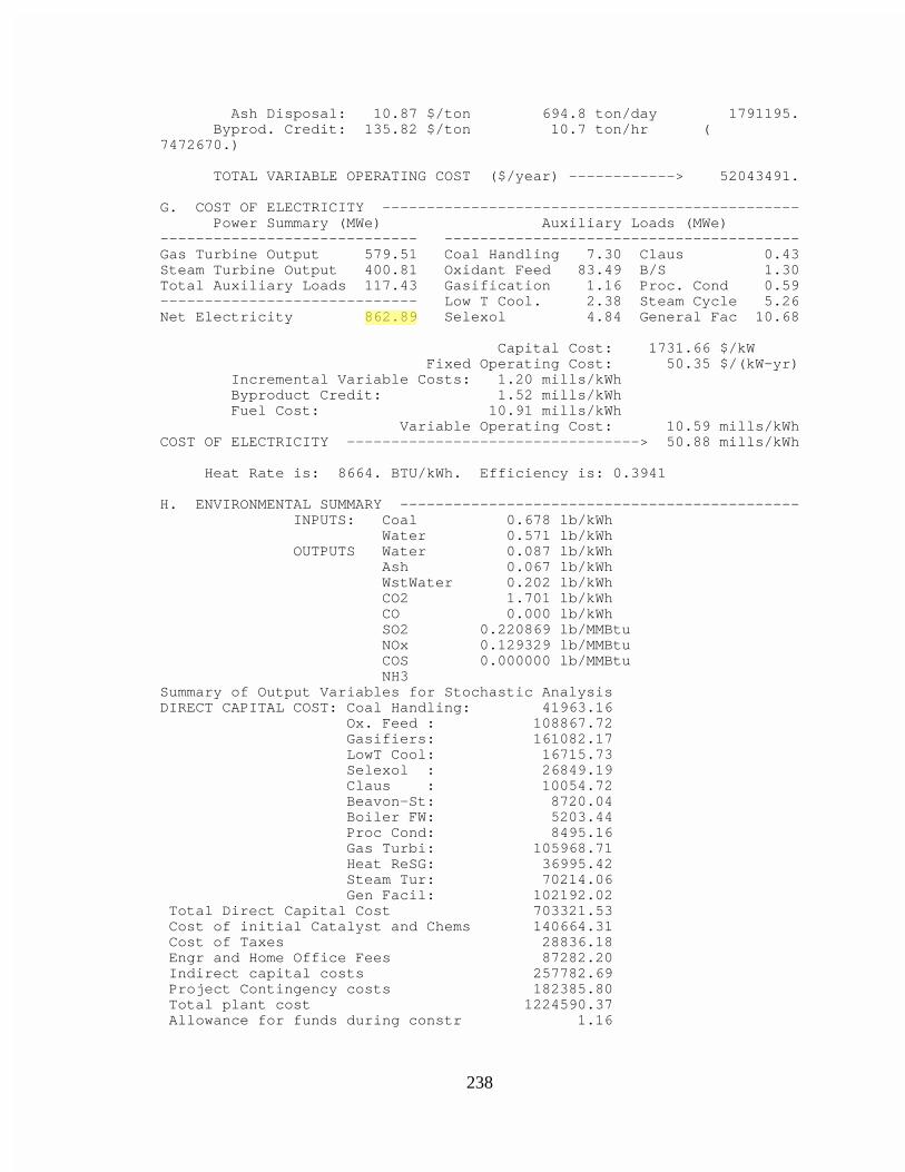
238
Ash Disposal: 10.87 $/ton 694.8 ton/day 1791195. Byprod. Credit: 135.82 $/ton 10.7 ton/hr (7472670.)
TOTAL VARIABLE OPERATING COST ($/year) ------------> 52043491.
G. COST OF ELECTRICITY ----------------------------------------------- Power Summary (MWe) Auxiliary Loads (MWe)----------------------------- ----------------------------------------Gas Turbine Output 579.51 Coal Handling 7.30 Claus 0.43Steam Turbine Output 400.81 Oxidant Feed 83.49 B/S 1.30Total Auxiliary Loads 117.43 Gasification 1.16 Proc. Cond 0.59----------------------------- Low T Cool. 2.38 Steam Cycle 5.26Net Electricity 862.89 Selexol 4.84 General Fac 10.68
Capital Cost: 1731.66 $/kW Fixed Operating Cost: 50.35 $/(kW-yr) Incremental Variable Costs: 1.20 mills/kWh Byproduct Credit: 1.52 mills/kWh Fuel Cost: 10.91 mills/kWh Variable Operating Cost: 10.59 mills/kWhCOST OF ELECTRICITY ---------------------------------> 50.88 mills/kWh
Heat Rate is: 8664. BTU/kWh. Efficiency is: 0.3941
H. ENVIRONMENTAL SUMMARY --------------------------------------------- INPUTS: Coal 0.678 lb/kWh Water 0.571 lb/kWh OUTPUTS Water 0.087 lb/kWh Ash 0.067 lb/kWh WstWater 0.202 lb/kWh CO2 1.701 lb/kWh CO 0.000 lb/kWh SO2 0.220869 lb/MMBtu NOx 0.129329 lb/MMBtu COS 0.000000 lb/MMBtu NH3Summary of Output Variables for Stochastic AnalysisDIRECT CAPITAL COST: Coal Handling: 41963.16 Ox. Feed : 108867.72 Gasifiers: 161082.17 LowT Cool: 16715.73 Selexol : 26849.19 Claus : 10054.72 Beavon-St: 8720.04 Boiler FW: 5203.44 Proc Cond: 8495.16 Gas Turbi: 105968.71 Heat ReSG: 36995.42 Steam Tur: 70214.06 Gen Facil: 102192.02 Total Direct Capital Cost 703321.53 Cost of initial Catalyst and Chems 140664.31 Cost of Taxes 28836.18 Engr and Home Office Fees 87282.20 Indirect capital costs 257782.69 Project Contingency costs 182385.80 Total plant cost 1224590.37 Allowance for funds during constr 1.16
Administrator
862.89
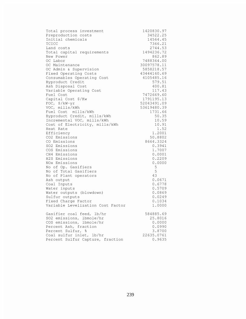
239
Total process investment 1420830.97 Preproduction costs 34522.25 Initial chemicals 14564.45 TCICC 7366.21 Land costs 2744.53 Total capital requirements 1494236.72 New Power 862.89 OC Labor 7488364.00 OC Maintenance 30097578.11 OC Admin & Supervision 5858218.57 Fixed Operating Costs 43444160.69 Consumables Operating Cost 4105485.16 Byproduct Credit 579.51 Ash Disposal Cost 400.81 Variable Operating Cost 117.43 Fuel Cost 7472669.60 Capital Cost $/Kw 1791195.13 FOC, $/kW-yr 52043491.09 VOC, mills/kWh 53619480.39 Fuel Cost mills/kWh 1731.66 Byproduct Credit, mills/kWh 50.35 Incremental VOC, mills/kWh 10.59 Cost of Electricity, mills/kWh 10.91 Heat Rate 1.52 Efficiency 1.2001 CO2 Emissions 50.8802 CO Emissions 8664.3324 SO2 Emissions 0.3941 COS Emissions 1.7007 CH4 Emissions 0.0001 H2S Emissions 0.2209 NOx Emissions 0.0000 No of Op. Gasifiers 5 No of Total Gasifiers 5 No of Plant operators 43 Ash output 0.0671 Coal Inputs 0.6778 Water inputs 0.5709 Water outputs (blowdown) 0.0869 Sulfur outputs 0.0249 Fixed Charge Factor 0.1034 Variable Levelization Cost Factor 1.0000
Gasifier coal feed, lb/hr 584885.69 SO2 emissions, lbmole/hr 25.8016 COS emissions, lbmole/hr 0.0000 Percent Ash, fraction 0.0990 Percent Sulfur, % 3.8700 Coal sulfur inlet, lb/hr 22635.0761 Percent Sulfur Capture, fraction 0.9635
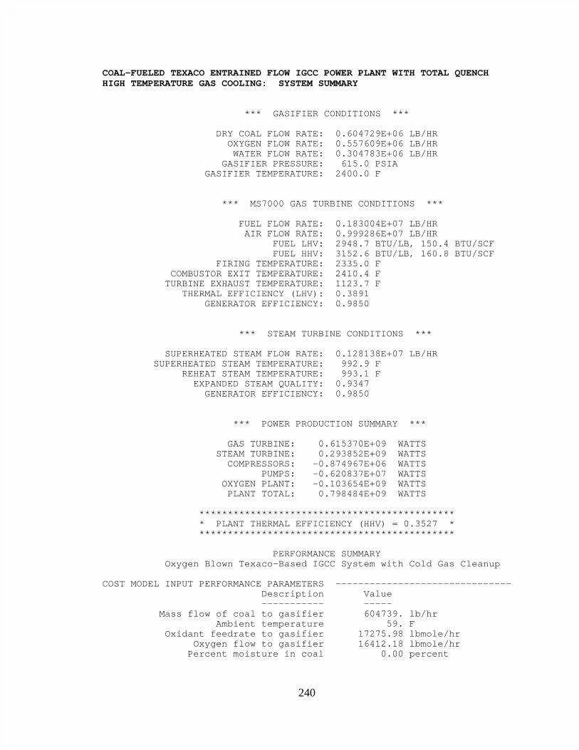
240
COAL-FUELED TEXACO ENTRAINED FLOW IGCC POWER PLANT WITH TOTAL QUENCHHIGH TEMPERATURE GAS COOLING: SYSTEM SUMMARY
*** GASIFIER CONDITIONS ***
DRY COAL FLOW RATE: 0.604729E+06 LB/HR OXYGEN FLOW RATE: 0.557609E+06 LB/HR WATER FLOW RATE: 0.304783E+06 LB/HR GASIFIER PRESSURE: 615.0 PSIA GASIFIER TEMPERATURE: 2400.0 F
*** MS7000 GAS TURBINE CONDITIONS ***
FUEL FLOW RATE: 0.183004E+07 LB/HR AIR FLOW RATE: 0.999286E+07 LB/HR FUEL LHV: 2948.7 BTU/LB, 150.4 BTU/SCF FUEL HHV: 3152.6 BTU/LB, 160.8 BTU/SCF FIRING TEMPERATURE: 2335.0 F COMBUSTOR EXIT TEMPERATURE: 2410.4 F TURBINE EXHAUST TEMPERATURE: 1123.7 F THERMAL EFFICIENCY (LHV): 0.3891 GENERATOR EFFICIENCY: 0.9850
*** STEAM TURBINE CONDITIONS ***
SUPERHEATED STEAM FLOW RATE: 0.128138E+07 LB/HR SUPERHEATED STEAM TEMPERATURE: 992.9 F REHEAT STEAM TEMPERATURE: 993.1 F EXPANDED STEAM QUALITY: 0.9347 GENERATOR EFFICIENCY: 0.9850
*** POWER PRODUCTION SUMMARY ***
GAS TURBINE: 0.615370E+09 WATTS STEAM TURBINE: 0.293852E+09 WATTS COMPRESSORS: -0.874967E+06 WATTS PUMPS: -0.620837E+07 WATTS OXYGEN PLANT: -0.103654E+09 WATTS PLANT TOTAL: 0.798484E+09 WATTS
********************************************* * PLANT THERMAL EFFICIENCY (HHV) = 0.3527 * *********************************************
PERFORMANCE SUMMARY Oxygen Blown Texaco-Based IGCC System with Cold Gas Cleanup
COST MODEL INPUT PERFORMANCE PARAMETERS ------------------------------- Description Value ----------- ----- Mass flow of coal to gasifier 604739. lb/hr Ambient temperature 59. F Oxidant feedrate to gasifier 17275.98 lbmole/hr Oxygen flow to gasifier 16412.18 lbmole/hr Percent moisture in coal 0.00 percent
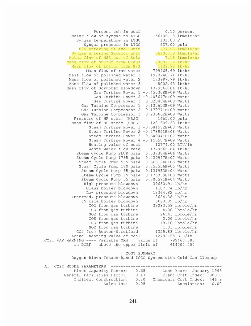
241
Percent ash in coal 0.10 percent Molar flow of syngas to LTGC 56106.18 lbmole/hr Syngas temperature in LTGC 101.00 F Syngas pressure in LTGC 537.00 psia H2S entering Selexol unit 677.58 lbmole/hr Syngas entering Selexol unit 56106.18 lbmole/hr Molar flow of H2S out of Selx 7.18 lbmole/hr Mass flow of sulfur from Claus 20681.16 lb/hr Mass flow of sulfur from B/S 1139.98 lb/hr Mass flow of raw water 799465.69 lb/hr Mass flow of polished water 1 1923748.71 lb/hr Mass flow of polished water 2 173997.79 lb/hr Mass flow of polished water 3 8002.93 lb/hr Mass flow of Scrubber Blowdown 1379566.84 lb/hr Gas Turbine Power 1 -0.450308E+09 Watts Gas Turbine Power 2 -0.405647E+09 Watts Gas Turbine Power 3 -0.320454E+09 Watts Gas Turbine Compressor 1 0.135653E+09 Watts Gas Turbine Compressor 2 0.179771E+09 Watts Gas Turbine Compressor 3 0.236662E+09 Watts Pressure of HP steam (HRSG) 1465.00 psia Mass flow of HP steam (HRSG) 1281399.33 lb/hr Steam Turbine Power 1 -0.581552E+08 Watts Steam Turbine Power 2 -0.778951E+08 Watts Steam Turbine Power 3 -0.649041E+07 Watts Steam Turbine Power 4 -0.155587E+09 Watts Heating value of coal 12774.00 BTU/lb Waste water flow rate 1379566.84 lb/hr Steam Cycle Pump SLUR psia 0.337384E+06 Watts Steam Cycle Pump 1785 psia 0.439947E+07 Watts Steam Cycle Pump 565 psia 0.363124E+05 Watts Steam Cycle Pump 180 psia 0.753556E+05 Watts Steam Cycle Pump 65 psia 0.131953E+04 Watts Steam Cycle Pump 25 psia 0.475339E+05 Watts Steam Cycle Pump 55 psia 0.705571E+04 Watts High pressure blowdown 39630.91 lb/hr Claus boiler blowdown 1187.74 lb/hr Low pressure blowdown 12364.82 lb/hr Intermed. pressure blowdown 8624.38 lb/hr 55 psia boiler blowdown 5628.89 lb/hr CO2 from gas turbine 33083.58 lbmole/hr CO from gas turbine 4.00 lbmole/hr SO2 from gas turbine 26.43 lbmole/hr COS from gas turbine 0.00 lbmole/hr NO from gas turbine 19.10 lbmole/hr NO2 from gas turbine 1.01 lbmole/hr CO2 from Beavon-Stretford 1355.88 lbmole/hr Actual heating value of coal 12782.65 BTU/lbCOST VAR WARNING ---- Variable MRW value of 799465.686 in DCBF above the upper limit of 614000.000
COST SUMMARY Oxygen Blown Texaco-Based IGCC System with Cold Gas Cleanup
A. COST MODEL PARAMETERS --------------------------------------------- Plant Capacity Factor: 0.65 Cost Year: January 1998 General Facilities Factor: 0.17 Plant Cost Index: 388.0 Indirect Construction: 0.20 Chemicals Cost Index: 446.8 Sales Tax: 0.05 Escalation: 0.00
Administrator
H2S entering Selexol unit 677.58 lbmole/hr
Administrator
Molar flow of H2S out of Selx 7.18 lbmole/hr
Administrator
Syngas entering Selexol unit 56106.18 lbmole/hr
Administrator
Mass flow of sulfur from Claus 20681.16 lb/hr
Administrator
Mass flow of sulfur from B/S 1139.98 lb/hr
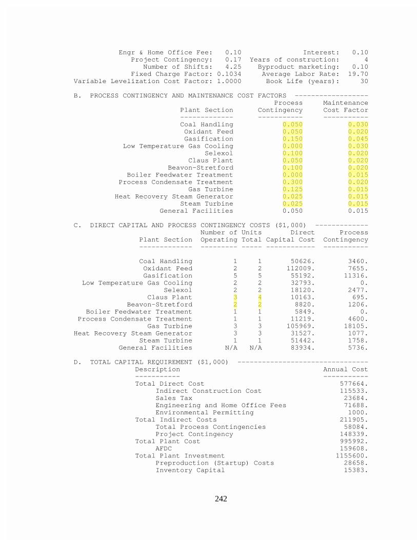
242
Engr & Home Office Fee: 0.10 Interest: 0.10 Project Contingency: 0.17 Years of construction: 4 Number of Shifts: 4.25 Byproduct marketing: 0.10 Fixed Charge Factor: 0.1034 Average Labor Rate: 19.70Variable Levelization Cost Factor: 1.0000 Book Life (years): 30
B. PROCESS CONTINGENCY AND MAINTENANCE COST FACTORS ------------------ Process Maintenance Plant Section Contingency Cost Factor ------------- ----------- ----------- Coal Handling 0.050 0.030 Oxidant Feed 0.050 0.020 Gasification 0.150 0.045 Low Temperature Gas Cooling 0.000 0.030 Selexol 0.100 0.020 Claus Plant 0.050 0.020 Beavon-Stretford 0.100 0.020 Boiler Feedwater Treatment 0.000 0.015 Process Condensate Treatment 0.300 0.020 Gas Turbine 0.125 0.015 Heat Recovery Steam Generator 0.025 0.015 Steam Turbine 0.025 0.015 General Facilities 0.050 0.015
C. DIRECT CAPITAL AND PROCESS CONTINGENCY COSTS ($1,000) ------------- Number of Units Direct Process Plant Section Operating Total Capital Cost Contingency ------------- --------- ----- ------------ -----------
Coal Handling 1 1 50626. 3460. Oxidant Feed 2 2 112009. 7655. Gasification 5 5 55192. 11316. Low Temperature Gas Cooling 2 2 32793. 0. Selexol 2 2 18120. 2477. Claus Plant 3 4 10163. 695. Beavon-Stretford 2 2 8820. 1206. Boiler Feedwater Treatment 1 1 5849. 0. Process Condensate Treatment 1 1 11219. 4600. Gas Turbine 3 3 105969. 18105.Heat Recovery Steam Generator 3 3 31527. 1077. Steam Turbine 1 1 51442. 1758. General Facilities N/A N/A 83934. 5736.
D. TOTAL CAPITAL REQUIREMENT ($1,000) -------------------------------- Description Annual Cost ----------- ----------- Total Direct Cost 577664. Indirect Construction Cost 115533. Sales Tax 23684. Engineering and Home Office Fees 71688. Environmental Permitting 1000. Total Indirect Costs 211905. Total Process Contingencies 58084. Project Contingency 148339. Total Plant Cost 995992. AFDC 159608. Total Plant Investment 1155600. Preproduction (Startup) Costs 28658. Inventory Capital 15383.
Administrator
3
Administrator
4
Administrator
2
Administrator
2
Administrator
0.030
Administrator
0.045
Administrator
0.030
Administrator
0.050
Administrator
0.050
Administrator
0.150
Administrator
0.000
Administrator
0.020
Administrator
0.100
Administrator
0.050
Administrator
0.100
Administrator
0.020
Administrator
0.020
Administrator
0.020
Administrator
0.125
Administrator
0.025
Administrator
0.025
Administrator
0.000
Administrator
0.300
Administrator
0.015
Administrator
0.020
Administrator
0.015
Administrator
0.015
Administrator
0.015
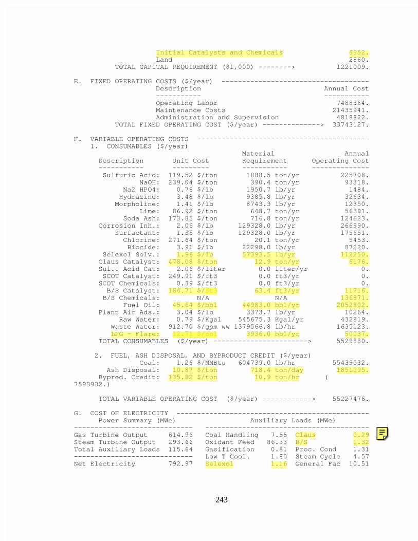
243
Initial Catalysts and Chemicals 6952. Land 2860. TOTAL CAPITAL REQUIREMENT ($1,000) --------> 1221009.
E. FIXED OPERATING COSTS ($/year) ------------------------------------ Description Annual Cost ----------- ----------- Operating Labor 7488364. Maintenance Costs 21435941. Administration and Supervision 4818822. TOTAL FIXED OPERATING COST ($/year) --------------> 33743127.
F. VARIABLE OPERATING COSTS ------------------------------------------ 1. CONSUMABLES ($/year) Material Annual Description Unit Cost Requirement Operating Cost ----------- --------- ----------- -------------- Sulfuric Acid: 119.52 $/ton 1888.5 ton/yr 225708. NaOH: 239.04 $/ton 390.4 ton/yr 93318. Na2 HPO4: 0.76 $/lb 1950.7 lb/yr 1484. Hydrazine: 3.48 $/lb 9385.8 lb/yr 32634. Morpholine: 1.41 $/lb 8743.3 lb/yr 12350. Lime: 86.92 $/ton 648.7 ton/yr 56391. Soda Ash: 173.85 $/ton 716.8 ton/yr 124623. Corrosion Inh.: 2.06 $/lb 129328.0 lb/yr 266990. Surfactant: 1.36 $/lb 129328.0 lb/yr 175651. Chlorine: 271.64 $/ton 20.1 ton/yr 5453. Biocide: 3.91 $/lb 22298.0 lb/yr 87220. Selexol Solv.: 1.96 $/lb 57393.5 lb/yr 112250. Claus Catalyst: 478.08 $/ton 12.9 ton/yr 6176. Sul.. Acid Cat: 2.06 $/liter 0.0 liter/yr 0. SCOT Catalyst: 249.91 $/ft3 0.0 ft3/yr 0. SCOT Chemicals: 0.39 $/ft3 0.0 ft3/yr 0. B/S Catalyst: 184.71 $/ft3 63.4 ft3/yr 11716. B/S Chemicals: N/A N/A 136871. Fuel Oil: 45.64 $/bbl 44983.0 bbl/yr 2052802. Plant Air Ads.: 3.04 $/lb 3373.7 lb/yr 10264. Raw Water: 0.79 $/Kgal 545675.3 Kgal/yr 432819. Waste Water: 912.70 $/gpm ww 1379566.8 lb/hr 1635123. LPG - Flare: 12.71 $/bbl 3936.0 bbl/yr 50037. TOTAL CONSUMABLES ($/year) -----------------------> 5529880.
2. FUEL, ASH DISPOSAL, AND BYPRODUCT CREDIT ($/year) Coal: 1.26 $/MMBtu 604739.0 lb/hr 55439532. Ash Disposal: 10.87 $/ton 718.4 ton/day 1851995. Byprod. Credit: 135.82 $/ton 10.9 ton/hr (7593932.)
TOTAL VARIABLE OPERATING COST ($/year) ------------> 55227476.
G. COST OF ELECTRICITY ----------------------------------------------- Power Summary (MWe) Auxiliary Loads (MWe)----------------------------- ----------------------------------------Gas Turbine Output 614.96 Coal Handling 7.55 Claus 0.29Steam Turbine Output 293.66 Oxidant Feed 86.33 B/S 1.32Total Auxiliary Loads 115.64 Gasification 0.81 Proc. Cond 1.31----------------------------- Low T Cool. 1.80 Steam Cycle 4.57Net Electricity 792.97 Selexol 1.16 General Fac 10.51
Administrator
B/S 1.32
Administrator
Claus load and Selexol load do not match between spreadsheet and these results. Equations in Excel used and flow rates from this report.
Administrator
Claus 0.29
Administrator
1.16
Administrator
Selexol
Administrator
184.71 $/ft3
Administrator
ft3 63.4 ft3/yr 11716.
Administrator
136871.
Administrator
45.64 $/bbl
Administrator
44983.0 bbl/yr
Administrator
2052802.
Administrator
12.71 $/bbl
Administrator
LPG - Flare: 12.71 $/bbl 3936.0 bbl/yr
Administrator
50037.
Administrator
135.82 $/ton
Administrator
10.9 ton/hr
Administrator
10.87 $/ton
Administrator
718.4 ton/day
Administrator
1851995.
Administrator
478.08 $/ton
Administrator
12.9 ton/yr
Administrator
6176.
Administrator
1.96 $/lb
Administrator
57393.5 lb/yr
Administrator
112250.
Administrator
Initial Catalysts and Chemicals 6952.
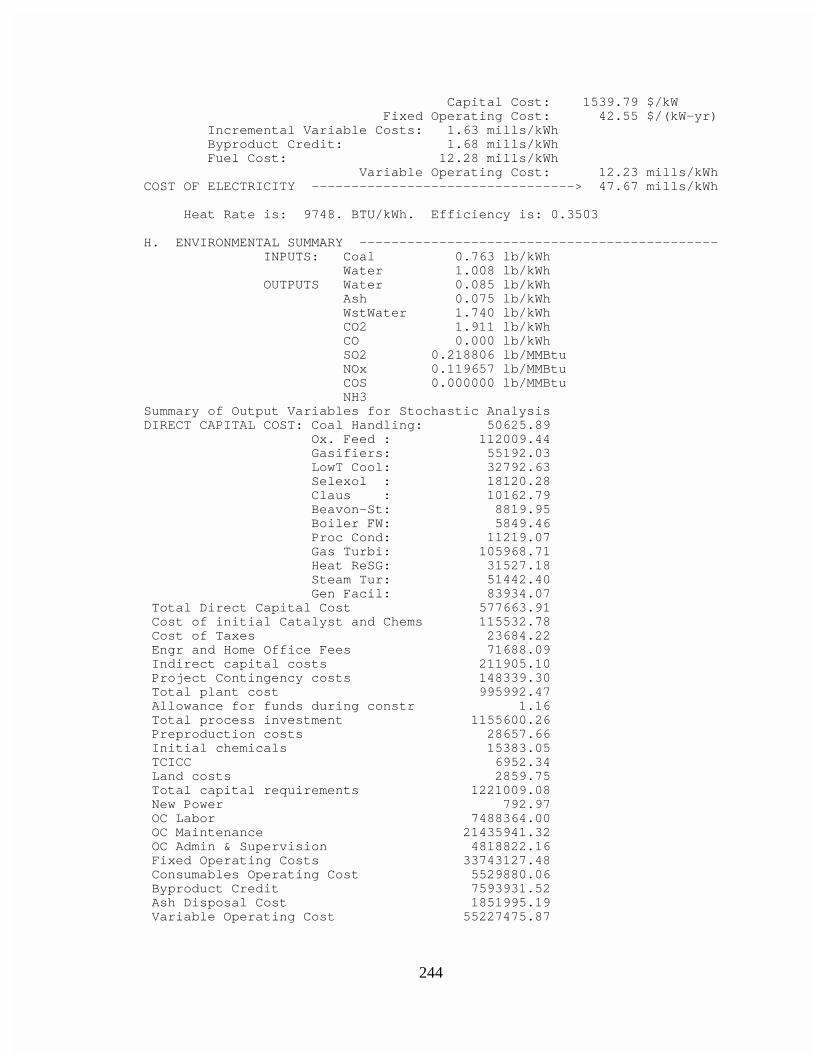
244
Capital Cost: 1539.79 $/kW Fixed Operating Cost: 42.55 $/(kW-yr) Incremental Variable Costs: 1.63 mills/kWh Byproduct Credit: 1.68 mills/kWh Fuel Cost: 12.28 mills/kWh Variable Operating Cost: 12.23 mills/kWhCOST OF ELECTRICITY ---------------------------------> 47.67 mills/kWh
Heat Rate is: 9748. BTU/kWh. Efficiency is: 0.3503
H. ENVIRONMENTAL SUMMARY --------------------------------------------- INPUTS: Coal 0.763 lb/kWh Water 1.008 lb/kWh OUTPUTS Water 0.085 lb/kWh Ash 0.075 lb/kWh WstWater 1.740 lb/kWh CO2 1.911 lb/kWh CO 0.000 lb/kWh SO2 0.218806 lb/MMBtu NOx 0.119657 lb/MMBtu COS 0.000000 lb/MMBtu NH3Summary of Output Variables for Stochastic AnalysisDIRECT CAPITAL COST: Coal Handling: 50625.89 Ox. Feed : 112009.44 Gasifiers: 55192.03 LowT Cool: 32792.63 Selexol : 18120.28 Claus : 10162.79 Beavon-St: 8819.95 Boiler FW: 5849.46 Proc Cond: 11219.07 Gas Turbi: 105968.71 Heat ReSG: 31527.18 Steam Tur: 51442.40 Gen Facil: 83934.07 Total Direct Capital Cost 577663.91 Cost of initial Catalyst and Chems 115532.78 Cost of Taxes 23684.22 Engr and Home Office Fees 71688.09 Indirect capital costs 211905.10 Project Contingency costs 148339.30 Total plant cost 995992.47 Allowance for funds during constr 1.16 Total process investment 1155600.26 Preproduction costs 28657.66 Initial chemicals 15383.05 TCICC 6952.34 Land costs 2859.75 Total capital requirements 1221009.08 New Power 792.97 OC Labor 7488364.00 OC Maintenance 21435941.32 OC Admin & Supervision 4818822.16 Fixed Operating Costs 33743127.48 Consumables Operating Cost 5529880.06 Byproduct Credit 7593931.52 Ash Disposal Cost 1851995.19 Variable Operating Cost 55227475.87
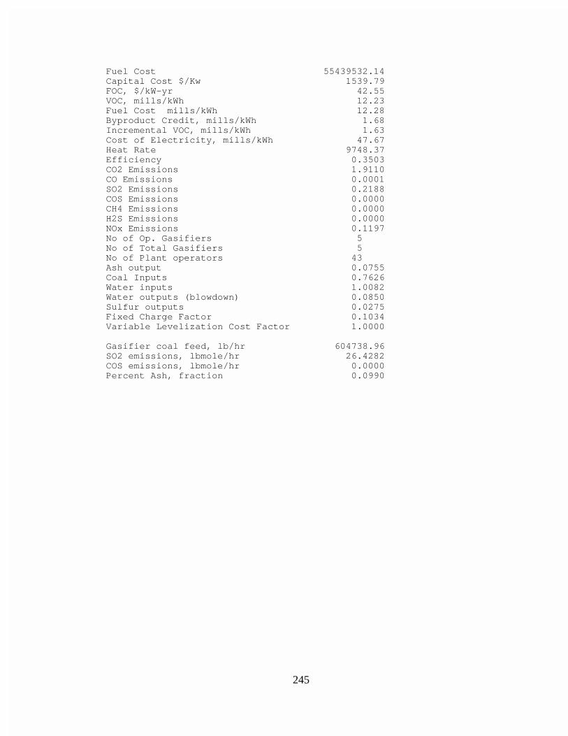
245
Fuel Cost 55439532.14 Capital Cost $/Kw 1539.79 FOC, $/kW-yr 42.55 VOC, mills/kWh 12.23 Fuel Cost mills/kWh 12.28 Byproduct Credit, mills/kWh 1.68 Incremental VOC, mills/kWh 1.63 Cost of Electricity, mills/kWh 47.67 Heat Rate 9748.37 Efficiency 0.3503 CO2 Emissions 1.9110 CO Emissions 0.0001 SO2 Emissions 0.2188 COS Emissions 0.0000 CH4 Emissions 0.0000 H2S Emissions 0.0000 NOx Emissions 0.1197 No of Op. Gasifiers 5 No of Total Gasifiers 5 No of Plant operators 43 Ash output 0.0755 Coal Inputs 0.7626 Water inputs 1.0082 Water outputs (blowdown) 0.0850 Sulfur outputs 0.0275 Fixed Charge Factor 0.1034 Variable Levelization Cost Factor 1.0000
Gasifier coal feed, lb/hr 604738.96 SO2 emissions, lbmole/hr 26.4282 COS emissions, lbmole/hr 0.0000 Percent Ash, fraction 0.0990
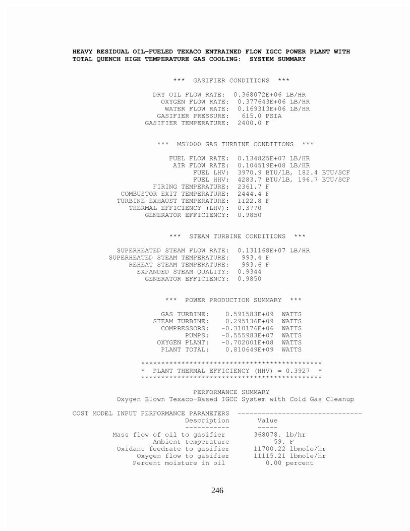
246
HEAVY RESIDUAL OIL-FUELED TEXACO ENTRAINED FLOW IGCC POWER PLANT WITHTOTAL QUENCH HIGH TEMPERATURE GAS COOLING: SYSTEM SUMMARY
*** GASIFIER CONDITIONS ***
DRY OIL FLOW RATE: 0.368072E+06 LB/HR OXYGEN FLOW RATE: 0.377643E+06 LB/HR WATER FLOW RATE: 0.169313E+06 LB/HR GASIFIER PRESSURE: 615.0 PSIA GASIFIER TEMPERATURE: 2400.0 F
*** MS7000 GAS TURBINE CONDITIONS ***
FUEL FLOW RATE: 0.134825E+07 LB/HR AIR FLOW RATE: 0.104519E+08 LB/HR FUEL LHV: 3970.9 BTU/LB, 182.4 BTU/SCF FUEL HHV: 4283.7 BTU/LB, 196.7 BTU/SCF FIRING TEMPERATURE: 2361.7 F COMBUSTOR EXIT TEMPERATURE: 2444.4 F TURBINE EXHAUST TEMPERATURE: 1122.8 F THERMAL EFFICIENCY (LHV): 0.3770 GENERATOR EFFICIENCY: 0.9850
*** STEAM TURBINE CONDITIONS ***
SUPERHEATED STEAM FLOW RATE: 0.131168E+07 LB/HR SUPERHEATED STEAM TEMPERATURE: 993.4 F REHEAT STEAM TEMPERATURE: 993.6 F EXPANDED STEAM QUALITY: 0.9344 GENERATOR EFFICIENCY: 0.9850
*** POWER PRODUCTION SUMMARY ***
GAS TURBINE: 0.591583E+09 WATTS STEAM TURBINE: 0.295136E+09 WATTS COMPRESSORS: -0.310176E+06 WATTS PUMPS: -0.555983E+07 WATTS OXYGEN PLANT: -0.702001E+08 WATTS PLANT TOTAL: 0.810649E+09 WATTS
********************************************* * PLANT THERMAL EFFICIENCY (HHV) = 0.3927 * *********************************************
PERFORMANCE SUMMARY Oxygen Blown Texaco-Based IGCC System with Cold Gas Cleanup
COST MODEL INPUT PERFORMANCE PARAMETERS ------------------------------- Description Value ----------- ----- Mass flow of oil to gasifier 368078. lb/hr Ambient temperature 59. F Oxidant feedrate to gasifier 11700.22 lbmole/hr Oxygen flow to gasifier 11115.21 lbmole/hr Percent moisture in oil 0.00 percent
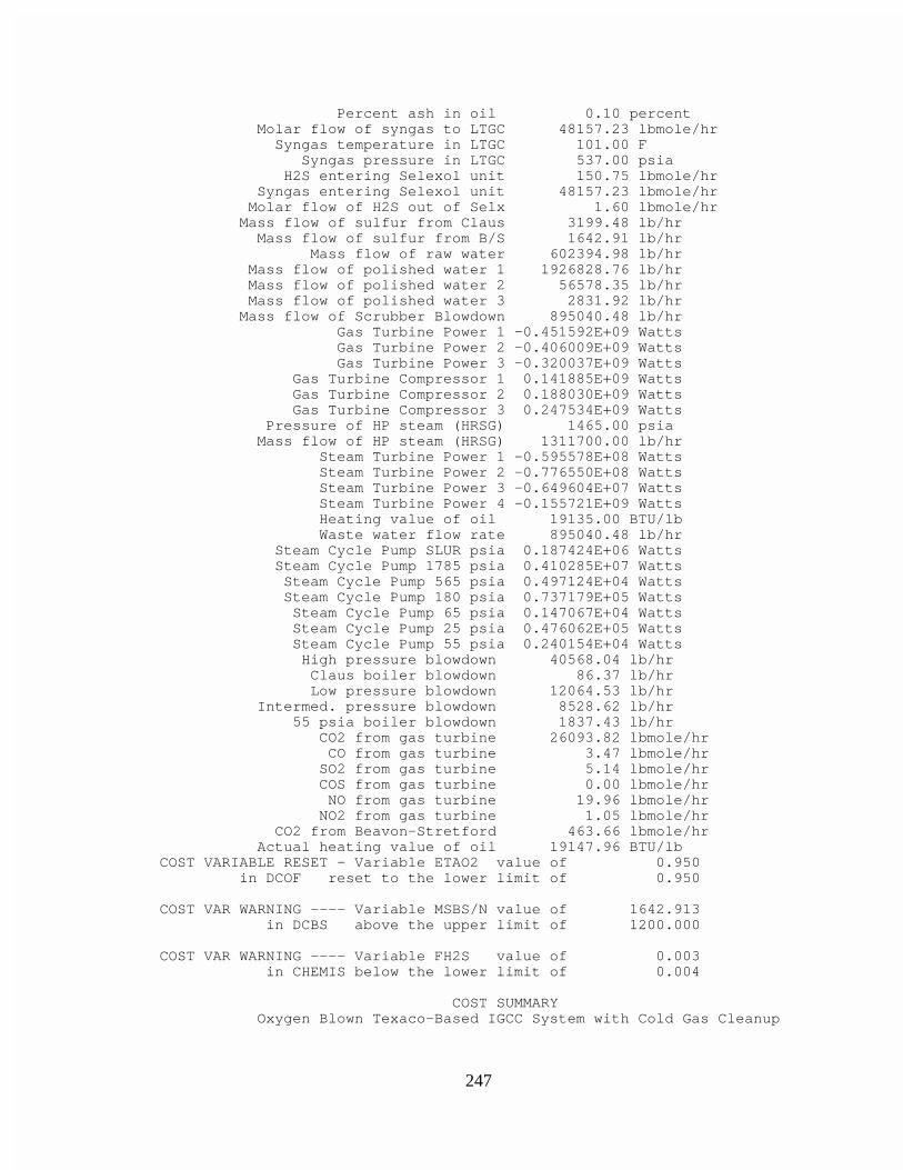
247
Percent ash in oil 0.10 percent Molar flow of syngas to LTGC 48157.23 lbmole/hr Syngas temperature in LTGC 101.00 F Syngas pressure in LTGC 537.00 psia H2S entering Selexol unit 150.75 lbmole/hr Syngas entering Selexol unit 48157.23 lbmole/hr Molar flow of H2S out of Selx 1.60 lbmole/hr Mass flow of sulfur from Claus 3199.48 lb/hr Mass flow of sulfur from B/S 1642.91 lb/hr Mass flow of raw water 602394.98 lb/hr Mass flow of polished water 1 1926828.76 lb/hr Mass flow of polished water 2 56578.35 lb/hr Mass flow of polished water 3 2831.92 lb/hr Mass flow of Scrubber Blowdown 895040.48 lb/hr Gas Turbine Power 1 -0.451592E+09 Watts Gas Turbine Power 2 -0.406009E+09 Watts Gas Turbine Power 3 -0.320037E+09 Watts Gas Turbine Compressor 1 0.141885E+09 Watts Gas Turbine Compressor 2 0.188030E+09 Watts Gas Turbine Compressor 3 0.247534E+09 Watts Pressure of HP steam (HRSG) 1465.00 psia Mass flow of HP steam (HRSG) 1311700.00 lb/hr Steam Turbine Power 1 -0.595578E+08 Watts Steam Turbine Power 2 -0.776550E+08 Watts Steam Turbine Power 3 -0.649604E+07 Watts Steam Turbine Power 4 -0.155721E+09 Watts Heating value of oil 19135.00 BTU/lb Waste water flow rate 895040.48 lb/hr Steam Cycle Pump SLUR psia 0.187424E+06 Watts Steam Cycle Pump 1785 psia 0.410285E+07 Watts Steam Cycle Pump 565 psia 0.497124E+04 Watts Steam Cycle Pump 180 psia 0.737179E+05 Watts Steam Cycle Pump 65 psia 0.147067E+04 Watts Steam Cycle Pump 25 psia 0.476062E+05 Watts Steam Cycle Pump 55 psia 0.240154E+04 Watts High pressure blowdown 40568.04 lb/hr Claus boiler blowdown 86.37 lb/hr Low pressure blowdown 12064.53 lb/hr Intermed. pressure blowdown 8528.62 lb/hr 55 psia boiler blowdown 1837.43 lb/hr CO2 from gas turbine 26093.82 lbmole/hr CO from gas turbine 3.47 lbmole/hr SO2 from gas turbine 5.14 lbmole/hr COS from gas turbine 0.00 lbmole/hr NO from gas turbine 19.96 lbmole/hr NO2 from gas turbine 1.05 lbmole/hr CO2 from Beavon-Stretford 463.66 lbmole/hr Actual heating value of oil 19147.96 BTU/lbCOST VARIABLE RESET - Variable ETAO2 value of 0.950 in DCOF reset to the lower limit of 0.950
COST VAR WARNING ---- Variable MSBS/N value of 1642.913 in DCBS above the upper limit of 1200.000
COST VAR WARNING ---- Variable FH2S value of 0.003 in CHEMIS below the lower limit of 0.004
COST SUMMARY Oxygen Blown Texaco-Based IGCC System with Cold Gas Cleanup
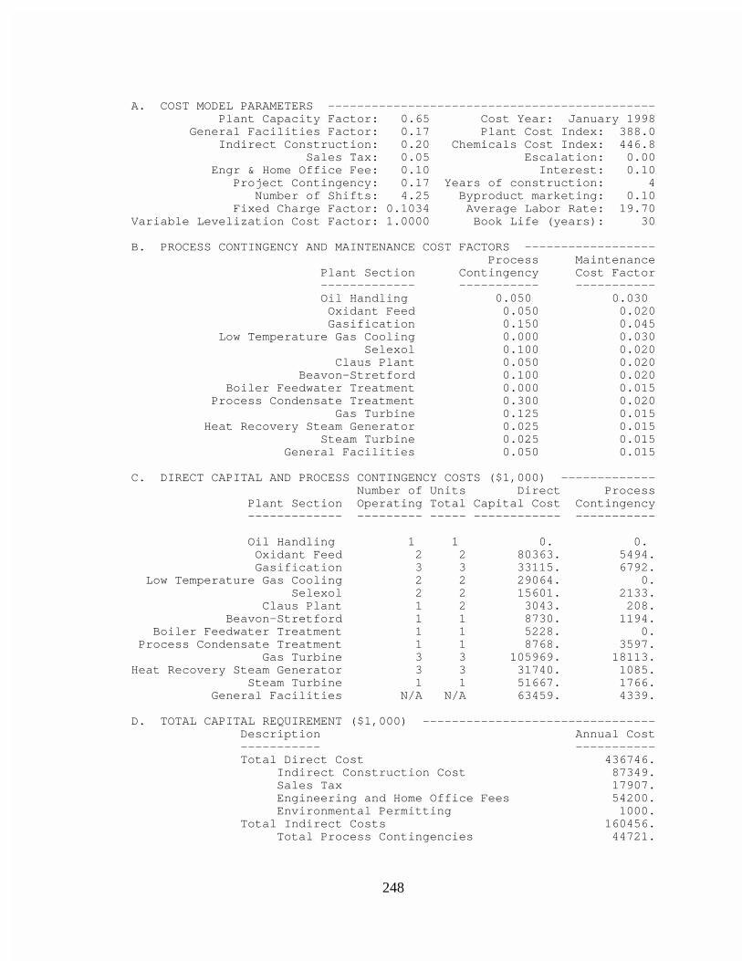
248
A. COST MODEL PARAMETERS --------------------------------------------- Plant Capacity Factor: 0.65 Cost Year: January 1998 General Facilities Factor: 0.17 Plant Cost Index: 388.0 Indirect Construction: 0.20 Chemicals Cost Index: 446.8 Sales Tax: 0.05 Escalation: 0.00 Engr & Home Office Fee: 0.10 Interest: 0.10 Project Contingency: 0.17 Years of construction: 4 Number of Shifts: 4.25 Byproduct marketing: 0.10 Fixed Charge Factor: 0.1034 Average Labor Rate: 19.70Variable Levelization Cost Factor: 1.0000 Book Life (years): 30
B. PROCESS CONTINGENCY AND MAINTENANCE COST FACTORS ------------------ Process Maintenance Plant Section Contingency Cost Factor ------------- ----------- ----------- Oil Handling 0.050 0.030 Oxidant Feed 0.050 0.020 Gasification 0.150 0.045 Low Temperature Gas Cooling 0.000 0.030 Selexol 0.100 0.020 Claus Plant 0.050 0.020 Beavon-Stretford 0.100 0.020 Boiler Feedwater Treatment 0.000 0.015 Process Condensate Treatment 0.300 0.020 Gas Turbine 0.125 0.015 Heat Recovery Steam Generator 0.025 0.015 Steam Turbine 0.025 0.015 General Facilities 0.050 0.015
C. DIRECT CAPITAL AND PROCESS CONTINGENCY COSTS ($1,000) ------------- Number of Units Direct Process Plant Section Operating Total Capital Cost Contingency ------------- --------- ----- ------------ -----------
Oil Handling 1 1 0. 0. Oxidant Feed 2 2 80363. 5494. Gasification 3 3 33115. 6792. Low Temperature Gas Cooling 2 2 29064. 0. Selexol 2 2 15601. 2133. Claus Plant 1 2 3043. 208. Beavon-Stretford 1 1 8730. 1194. Boiler Feedwater Treatment 1 1 5228. 0. Process Condensate Treatment 1 1 8768. 3597. Gas Turbine 3 3 105969. 18113.Heat Recovery Steam Generator 3 3 31740. 1085. Steam Turbine 1 1 51667. 1766. General Facilities N/A N/A 63459. 4339.
D. TOTAL CAPITAL REQUIREMENT ($1,000) -------------------------------- Description Annual Cost ----------- ----------- Total Direct Cost 436746. Indirect Construction Cost 87349. Sales Tax 17907. Engineering and Home Office Fees 54200. Environmental Permitting 1000. Total Indirect Costs 160456. Total Process Contingencies 44721.
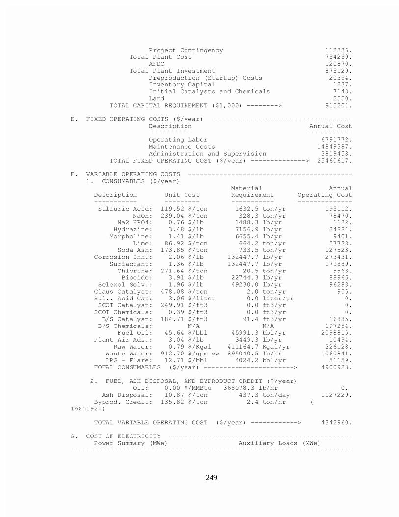
249
Project Contingency 112336. Total Plant Cost 754259. AFDC 120870. Total Plant Investment 875129. Preproduction (Startup) Costs 20394. Inventory Capital 1237. Initial Catalysts and Chemicals 7143. Land 2550. TOTAL CAPITAL REQUIREMENT ($1,000) --------> 915204.
E. FIXED OPERATING COSTS ($/year) ------------------------------------ Description Annual Cost ----------- ----------- Operating Labor 6791772. Maintenance Costs 14849387. Administration and Supervision 3819458. TOTAL FIXED OPERATING COST ($/year) --------------> 25460617.
F. VARIABLE OPERATING COSTS ------------------------------------------ 1. CONSUMABLES ($/year) Material Annual Description Unit Cost Requirement Operating Cost ----------- --------- ----------- -------------- Sulfuric Acid: 119.52 $/ton 1632.5 ton/yr 195112. NaOH: 239.04 $/ton 328.3 ton/yr 78470. Na2 HPO4: 0.76 $/lb 1488.3 lb/yr 1132. Hydrazine: 3.48 $/lb 7156.9 lb/yr 24884. Morpholine: 1.41 $/lb 6655.4 lb/yr 9401. Lime: 86.92 $/ton 664.2 ton/yr 57738. Soda Ash: 173.85 $/ton 733.5 ton/yr 127523. Corrosion Inh.: 2.06 $/lb 132447.7 lb/yr 273431. Surfactant: 1.36 $/lb 132447.7 lb/yr 179889. Chlorine: 271.64 $/ton 20.5 ton/yr 5563. Biocide: 3.91 $/lb 22744.3 lb/yr 88966. Selexol Solv.: 1.96 $/lb 49230.0 lb/yr 96283. Claus Catalyst: 478.08 $/ton 2.0 ton/yr 955. Sul.. Acid Cat: 2.06 $/liter 0.0 liter/yr 0. SCOT Catalyst: 249.91 $/ft3 0.0 ft3/yr 0. SCOT Chemicals: 0.39 $/ft3 0.0 ft3/yr 0. B/S Catalyst: 184.71 $/ft3 91.4 ft3/yr 16885. B/S Chemicals: N/A N/A 197254. Fuel Oil: 45.64 $/bbl 45991.3 bbl/yr 2098815. Plant Air Ads.: 3.04 $/lb 3449.3 lb/yr 10494. Raw Water: 0.79 $/Kgal 411164.7 Kgal/yr 326128. Waste Water: 912.70 $/gpm ww 895040.5 lb/hr 1060841. LPG - Flare: 12.71 $/bbl 4024.2 bbl/yr 51159. TOTAL CONSUMABLES ($/year) -----------------------> 4900923.
2. FUEL, ASH DISPOSAL, AND BYPRODUCT CREDIT ($/year) Oil: 0.00 $/MMBtu 368078.3 lb/hr 0. Ash Disposal: 10.87 $/ton 437.3 ton/day 1127229. Byprod. Credit: 135.82 $/ton 2.4 ton/hr (1685192.)
TOTAL VARIABLE OPERATING COST ($/year) ------------> 4342960.
G. COST OF ELECTRICITY ----------------------------------------------- Power Summary (MWe) Auxiliary Loads (MWe)----------------------------- ----------------------------------------
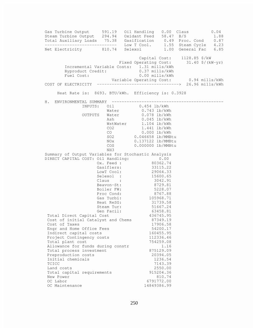
250
Gas Turbine Output 591.19 Oil Handling 0.00 Claus 0.04Steam Turbine Output 294.94 Oxidant Feed 58.47 B/S 1.88Total Auxiliary Loads 75.38 Gasification 0.49 Proc. Cond 0.87----------------------------- Low T Cool. 1.55 Steam Cycle 4.23Net Electricity 810.74 Selexol 1.00 General Fac 6.85
Capital Cost: 1128.85 $/kW Fixed Operating Cost: 31.40 $/(kW-yr) Incremental Variable Costs: 1.31 mills/kWh Byproduct Credit: 0.37 mills/kWh Fuel Cost: 0.00 mills/kWh Variable Operating Cost: 0.94 mills/kWhCOST OF ELECTRICITY ---------------------------------> 26.96 mills/kWh
Heat Rate is: 8693. BTU/kWh. Efficiency is: 0.3928
H. ENVIRONMENTAL SUMMARY --------------------------------------------- INPUTS: Oil 0.454 lb/kWh Water 0.743 lb/kWh OUTPUTS Water 0.078 lb/kWh Ash 0.045 lb/kWh WstWater 1.104 lb/kWh CO2 1.441 lb/kWh CO 0.000 lb/kWh SO2 0.046658 lb/MMBtu NOx 0.137122 lb/MMBtu COS 0.000000 lb/MMBtu NH3Summary of Output Variables for Stochastic AnalysisDIRECT CAPITAL COST: Oil Handling: 0.00 Ox. Feed : 80362.74 Gasifiers: 33115.22 LowT Cool: 29064.33 Selexol : 15600.65 Claus : 3042.91 Beavon-St: 8729.81 Boiler FW: 5228.07 Proc Cond: 8767.88 Gas Turbi: 105968.71 Heat ReSG: 31739.58 Steam Tur: 51667.24 Gen Facil: 63458.81 Total Direct Capital Cost 436745.95 Cost of initial Catalyst and Chems 87349.19 Cost of Taxes 17906.58 Engr and Home Office Fees 54200.17 Indirect capital costs 160455.95 Project Contingency costs 112336.46 Total plant cost 754259.08 Allowance for funds during constr 1.16 Total process investment 875129.09 Preproduction costs 20394.05 Initial chemicals 1236.54 TCICC 7143.39 Land costs 2550.00 Total capital requirements 915204.36 New Power 810.74 OC Labor 6791772.00 OC Maintenance 14849386.99
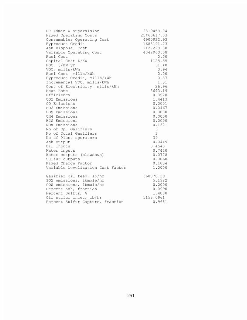
251
OC Admin & Supervision 3819458.04 Fixed Operating Costs 25460617.03 Consumables Operating Cost 4900922.93 Byproduct Credit 1685191.73 Ash Disposal Cost 1127228.88 Variable Operating Cost 4342960.08 Fuel Cost 0.00 Capital Cost $/Kw 1128.85 FOC, $/kW-yr 31.40 VOC, mills/kWh 0.94 Fuel Cost mills/kWh 0.00 Byproduct Credit, mills/kWh 0.37 Incremental VOC, mills/kWh 1.31 Cost of Electricity, mills/kWh 26.96 Heat Rate 8693.19 Efficiency 0.3928 CO2 Emissions 1.4413 CO Emissions 0.0001 SO2 Emissions 0.0467 COS Emissions 0.0000 CH4 Emissions 0.0000 H2S Emissions 0.0000 NOx Emissions 0.1371 No of Op. Gasifiers 3 No of Total Gasifiers 3 No of Plant operators 39 Ash output 0.0449 Oil Inputs 0.4540 Water inputs 0.7430 Water outputs (blowdown) 0.0778 Sulfur outputs 0.0060 Fixed Charge Factor 0.1034 Variable Levelization Cost Factor 1.0000
Gasifier oil feed, lb/hr 368078.29 SO2 emissions, lbmole/hr 5.1382 COS emissions, lbmole/hr 0.0000 Percent Ash, fraction 0.0990 Percent Sulfur, % 1.4000 Oil sulfur inlet, lb/hr 5153.0961 Percent Sulfur Capture, fraction 0.9681

252
APPENDIX C: PARTIAL RANK CORRELATION COEFFICIENTS FOR THE
IGCC SYSTEMS