20 Entropy and the Second Law of Thermodynamics
51
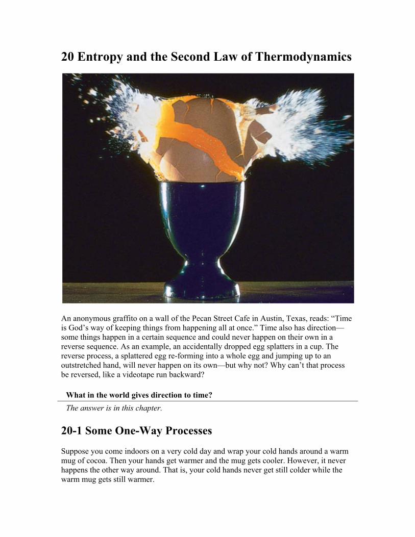
20 Entropy and the Second Law of Thermodynamics An anonymous graffito on a wall of the Pecan Street Cafe in Austin, Texas, reads: “Time is God’s way of keeping things from happening all at once.” Time also has direction— some things happen in a certain sequence and could never happen on their own in a reverse sequence. As an example, an accidentally dropped egg splatters in a cup. The reverse process, a splattered egg re-forming into a whole egg and jumping up to an outstretched hand, will never happen on its own—but why not? Why can’t that process be reversed, like a videotape run backward? What in the world gives direction to time? The answer is in this chapter. 20-1 Some One-Way Processes Suppose you come indoors on a very cold day and wrap your cold hands around a warm mug of cocoa. Then your hands get warmer and the mug gets cooler. However, it never happens the other way around. That is, your cold hands never get still colder while the warm mug gets still warmer.
Transcript of 20 Entropy and the Second Law of Thermodynamics
20 Entropy and the Second Law of Thermodynamics
An anonymous graffito on a wall of the Pecan Street Cafe in Austin, Texas, reads: “Time is God’s way of keeping things from happening all at once.” Time also has direction—some things happen in a certain sequence and could never happen on their own in a reverse sequence. As an example, an accidentally dropped egg splatters in a cup. The reverse process, a splattered egg re-forming into a whole egg and jumping up to an outstretched hand, will never happen on its own—but why not? Why can’t that process be reversed, like a videotape run backward?
What in the world gives direction to time?
The answer is in this chapter.
20-1 Some One-Way Processes
Suppose you come indoors on a very cold day and wrap your cold hands around a warm mug of cocoa. Then your hands get warmer and the mug gets cooler. However, it never happens the other way around. That is, your cold hands never get still colder while the warm mug gets still warmer.
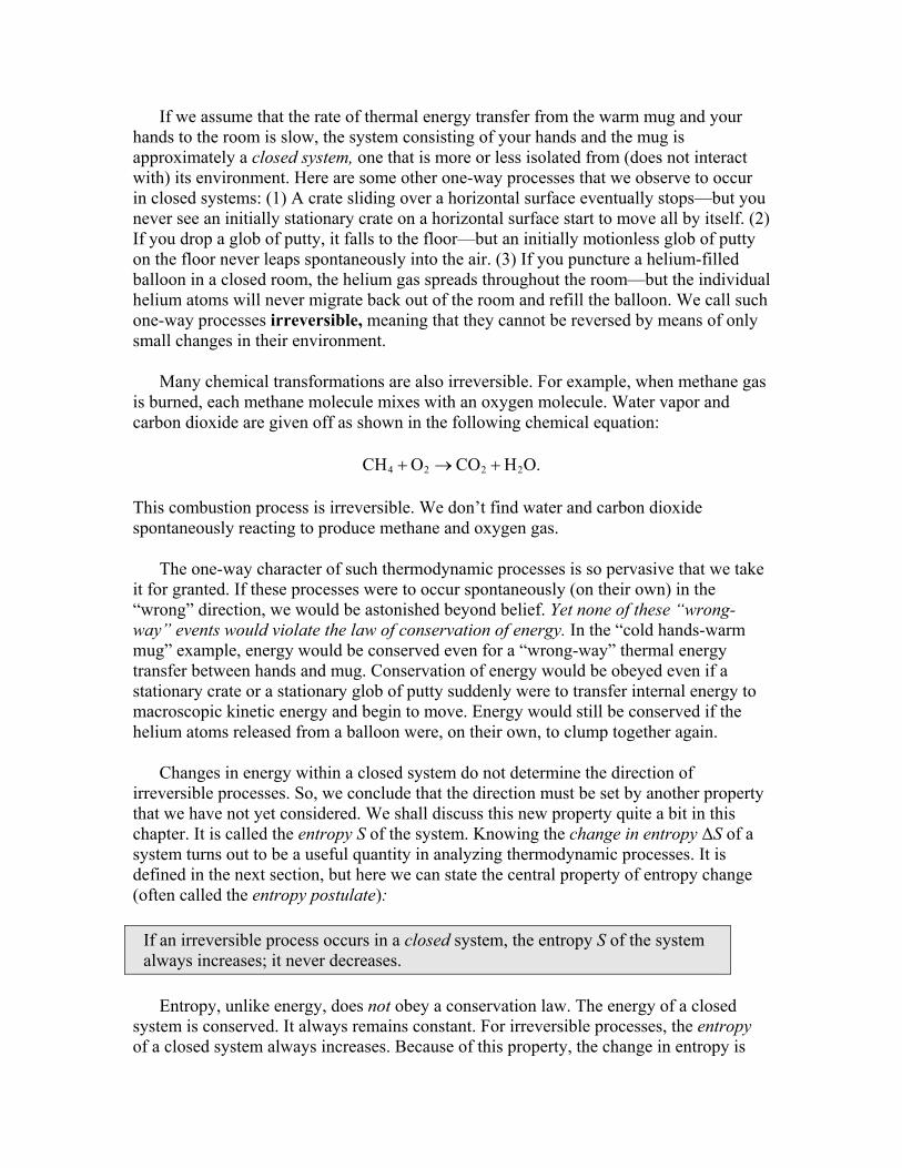
If we assume that the rate of thermal energy transfer from the warm mug and your hands to the room is slow, the system consisting of your hands and the mug is approximately a closed system, one that is more or less isolated from (does not interact with) its environment. Here are some other one-way processes that we observe to occur in closed systems: (1) A crate sliding over a horizontal surface eventually stops—but you never see an initially stationary crate on a horizontal surface start to move all by itself. (2) If you drop a glob of putty, it falls to the floor—but an initially motionless glob of putty on the floor never leaps spontaneously into the air. (3) If you puncture a helium-filled balloon in a closed room, the helium gas spreads throughout the room—but the individual helium atoms will never migrate back out of the room and refill the balloon. We call such one-way processes irreversible, meaning that they cannot be reversed by means of only small changes in their environment.
Many chemical transformations are also irreversible. For example, when methane gas is burned, each methane molecule mixes with an oxygen molecule. Water vapor and carbon dioxide are given off as shown in the following chemical equation:
4 2 2 2CH O CO H O.
This combustion process is irreversible. We don’t find water and carbon dioxide spontaneously reacting to produce methane and oxygen gas.
The one-way character of such thermodynamic processes is so pervasive that we take it for granted. If these processes were to occur spontaneously (on their own) in the “wrong” direction, we would be astonished beyond belief. Yet none of these “wrong-way” events would violate the law of conservation of energy. In the “cold hands-warm mug” example, energy would be conserved even for a “wrong-way” thermal energy transfer between hands and mug. Conservation of energy would be obeyed even if a stationary crate or a stationary glob of putty suddenly were to transfer internal energy to macroscopic kinetic energy and begin to move. Energy would still be conserved if the helium atoms released from a balloon were, on their own, to clump together again.
Changes in energy within a closed system do not determine the direction of irreversible processes. So, we conclude that the direction must be set by another property that we have not yet considered. We shall discuss this new property quite a bit in this chapter. It is called the entropy S of the system. Knowing the change in entropy ΔS of a system turns out to be a useful quantity in analyzing thermodynamic processes. It is defined in the next section, but here we can state the central property of entropy change (often called the entropy postulate):
If an irreversible process occurs in a closed system, the entropy S of the system always increases; it never decreases.
Entropy, unlike energy, does not obey a conservation law. The energy of a closed system is conserved. It always remains constant. For irreversible processes, the entropy of a closed system always increases. Because of this property, the change in entropy is
sometimes called “the arrow of time.” For example, we associate the irreversible breaking of the egg in our opening photograph with the forward direction of time and also with an increase in entropy. The backward direction of time (a videotape run backward) would correspond to the broken egg re-forming into a whole egg and rising into the air. This backward process would result in an entropy decrease and so it never happens.
There are two equivalent ways to define the change in entropy of a system. The first is macroscopic. It is in terms of the system’s temperature and any thermal energy transfers between the system and its surroundings. The second is macroscopic or statistical. It is defined by counting the ways in which the atoms or molecules that make up the system can be arranged. We use the first approach in the next section, and the second in Section 20-7.
READING EXERCISE 20-1: Consider the irreversible process of dropping a glob of putty on the floor. Describe what energy transformations are taking place that allow us to believe that energy is conserved.
READING EXERCISE 20-2: List additional everyday phenomena that illustrate irreversibility without violating energy conservation.
20-2 Change in Entropy
In this section, we will try to develop a definition for change in entropy by looking again at the macroscopic process that we described in Sections 19-8 and 20-10—namely, the free expansion of an ideal gas. Figure 20-1a shows the gas in its initial equilibrium state i, confined by a closed stopcock to the left half of a thermally insulated container. If we open the stopcock, the gas rushes to fill the entire container, eventually reaching the final equilibrium state f shown in Fig. 20-1b. Unless the number of gas molecules is small (which is very hard to accomplish), this is an irreversible process. Again, what we mean by irreversible is that it is extremely improbable that all the gas particles would return, by themselves, to the left half of the container.
The P-V plot of the process in Fig. 20-2 shows the pressure and volume of the gas in its initial state i and final state f. As we discuss in Section 19-1, the pressure and volume of the gas depend only on the state that the gas is in, and not on the process by which it arrived in that state. Therefore, pressure and volume are examples of state properties. State properties are properties that depend only on the state of the gas and not on how it reached that state. Other state properties are temperature and internal energy. We now assume that the gas has still another state property—its entropy. Furthermore, we define the change in entropy Sf − Si of a system during a process that takes the system from an initial state i to a final state f as

FIGURE 20-1 The free expansion of an ideal gas consisting of a large number of molecules. (a) The gas is confined to the left half of an insulated container by a closed stopcock. (b) When the stopcock is opened, the gas rushes to fill the entire container. This process is irreversible; that is, it is never observed to occur in reverse, with the gas spontaneously collecting itself in the left half of the container.
(change in entropy defined). (20-1)f
f ii
dQS S S
T
Here Q is the thermal energy transferred to or from the system during a heating or cooling process, and T is the temperature of the system in kelvin. Thus, an entropy change depends not only on the thermal energy transferred Q, but also on the temperature at which the transfer takes place. Because T is always positive, the sign of ΔS is the same as that of Q (positive if thermal energy is transferred to the system and negative if thermal energy is transferred from the system). We see from this relation (Eq. 20-1) that the SI unit for entropy and entropy change is the joule per kelvin.
There is a problem, however, in applying Eq. 20-1 to the free expansion of Fig. 20-1. As the gas rushes to fill the entire container, the pressure, temperature, and volume of the gas fluctuate unpredictably. In other words, they do not have a sequence of well-defined
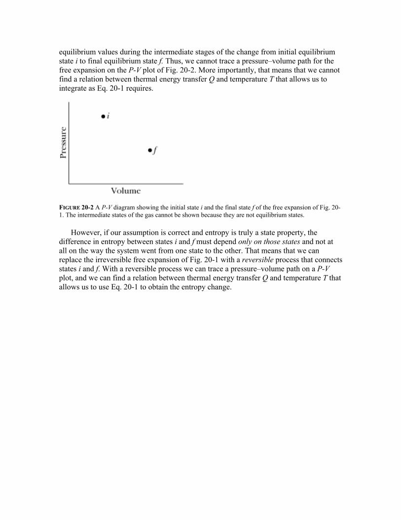
equilibrium values during the intermediate stages of the change from initial equilibrium state i to final equilibrium state f. Thus, we cannot trace a pressure–volume path for the free expansion on the P-V plot of Fig. 20-2. More importantly, that means that we cannot find a relation between thermal energy transfer Q and temperature T that allows us to integrate as Eq. 20-1 requires.
FIGURE 20-2 A P-V diagram showing the initial state i and the final state f of the free expansion of Fig. 20-1. The intermediate states of the gas cannot be shown because they are not equilibrium states.
However, if our assumption is correct and entropy is truly a state property, the difference in entropy between states i and f must depend only on those states and not at all on the way the system went from one state to the other. That means that we can replace the irreversible free expansion of Fig. 20-1 with a reversible process that connects states i and f. With a reversible process we can trace a pressure–volume path on a P-V plot, and we can find a relation between thermal energy transfer Q and temperature T that allows us to use Eq. 20-1 to obtain the entropy change.

FIGURE 20-3 The isothermal expansion of an ideal gas, done in a reversible way. The gas has the same initial state i and same final state f as in the irreversible process of Figs. 20-1 and 20-2.
We saw in Section 20-10 that the temperature of an ideal gas does not change during a free expansion. So, Ti = Tf = T. Thus, points i and f in Fig. 20-2 must be on the same isotherm. A convenient replacement process is then a reversible isothermal expansion

from state i to state f, which actually proceeds along that isotherm. Furthermore, because T is constant throughout a reversible isothermal expansion, the integral of Eq. 20-1 is greatly simplified.
Figure 20-3 shows how to produce such a reversible isothermal expansion. We confine the gas to an insulated cylinder that rests on a thermal reservoir maintained at the temperature T. We begin by placing just enough lead shot on the movable piston so that the pressure and volume of the gas are those of the initial state i of Fig. 20-1a. We then remove shot slowly (piece by piece) until the pressure and volume of the gas are those of the final state f of Fig. 20-1b. The temperature of the gas does not change because the gas remains in thermal contact with the reservoir throughout the process.
The reversible isothermal expansion of Fig. 20-3 is physically quite different from the irreversible free expansion of Fig. 20-1. However, both processes have the same initial state and the same final state. Thus, if entropy is a state property, these two processes must result in the same change in entropy.
Because we removed the lead shot slowly, the intermediate states of the gas are equilibrium states, so we can plot them on a P-V diagram (Fig. 20-4). To apply Eq. 20-1 to the isothermal expansion, we take the constant temperature T outside the integral, obtaining
1.
f
f ii
S S S dQT
Because ,dQ Q where Q is the thermal energy transferred during the process, we have
(change in entropy, isothermal process). (20-2)f iQ
S S ST
To keep the temperature T of the gas constant during the isothermal expansion of Fig. 20-3, the thermal energy transferred from the reservoir to the gas must have been Q. Thus, Q is positive and the entropy of the gas increases during the isothermal process and during the free expansion of Fig. 20-1.
To summarize:
Assuming entropy is a state property, we can find the entropy change for an irreversible process occurring in a closed system by replacing that process with any reversible process that connects the same initial and final states. We can then calculate the entropy change for this reversible process with Eq. 20-1. The change in entropy for an irreversible process connecting the same two states would be the same.

FIGURE 20 -4 A P-V diagram for the reversible isothermal expansion of Fig. 20-3. The intermediate states, which are now equilibrium states, are shown.
We can even use this approach if the temperature of the system is not quite constant. That is, if the temperature change ΔT of a system is small relative to the temperature (in kelvin) before and after the process, the entropy change can be approximated as
(20-3)f iQ
S S ST
where T is the average kelvin temperature of the system during the process.
Entropy as a State Property
In the previous section, we assumed that entropy, like pressure, internal energy, and temperature, is a property of the state of a system and is independent of how that state is reached. The fact that entropy is indeed a state property (or state function as state properties are sometimes called) can really only be deduced by careful experiment. However, we will prove entropy is a state property for the special and important case of an ideal gas undergoing a reversible process. This proof will serve two purposes. First, it will verify (for at least this one case) that entropy is a state property (or state function) as we assumed in the section above. Second, it will allow us to develop an expression for the entropy change in an ideal gas as it goes from some initial state i to some final state f via a reversible process.
To make the process reversible, we must make changes slowly in a series of small steps, with the ideal gas in an equilibrium state at the end of each step. For each small step, the thermal energy transfer to or from the gas is dQ, the work done by or on the gas is dW, and the change in internal energy is dEint. These are related by the first law of thermodynamics in differential form (Eq. 19-18):
int .dE dQ dW

Because the steps are reversible, with the gas in equilibrium states, we can replace dW with P dV (Eq. 19-15). Since we are dealing with an ideal gas, we can also replace dEint with nCV dT (Eq. 20-43). Solving for the thermal energy transferred to or from the system in a single small step of the process dQ then leads to
.VdQ PdV nC dT
We replace the pressure P in this equation with nRT/V (using the ideal gas law). Then we divide each term in the resulting equation by the temperature T, obtaining
.VdQ dV dT
nR nCT V T
Now let us integrate each term of this equation between an arbitrary initial state i and an arbitrary final state f to get
.f f f
Vi i i
dQ dV dTnR nC
T V T
The quantity on the left is the entropy change ΔS(= Sf − Si) as we defined it in Eq. 20-1. Substituting this and integrating the quantities on the right yields an expression for the entropy change in an ideal gas undergoing a reversible process:
ln ln . (20-4)f ff i V
i i
V TS S S nR nC
V T
Note that we did not have to specify a particular reversible process when we integrated. Therefore, the integration must hold for all reversible processes that take the gas from state i to state f. Thus, we see that the change in entropy ΔS between the initial and final states of an ideal gas does depend only on properties of the initial state (Vi and Ti) and properties of the final states (Vf and Tf ); ΔS does not depend on how the gas changes between the two equilibrium states. Therefore, in at least this one case, we know that entropy must be a state property. In the work that follows in this chapter, we will accept without further proof that entropy is in fact a state property for any system undergoing any process.
READING EXERCISE 20-3: Thermal energy is transferred to water on a stove. Rank the entropy changes of the water as its temperature rises (a) from 20°C to 30°C, (b) from 30°C to 35°C, and (c) from 80°C to 85°C, greatest first.

TOUCHSTONE EXAMPLE 20-1: Nitrogen
One mole of nitrogen gas is confined to the left side of the container of Fig. 20-1a. You open the stopcock and the volume of the gas doubles. What is the entropy change of the gas for this irreversible process? Treat the gas as ideal.
SOLUTION We need two Key Ideas here. One is that we can determine the entropy change for the irreversible process by calculating it for a reversible process that provides the same change in volume. The other is that the temperature of the gas does not change in the free expansion. Thus, the reversible process should be an isothermal expansion—namely, the one of Figs. 20-3 and 20-4.
Since the internal energy of an ideal gas depends only on temperature, ΔEint = 0 here and so Q = W from the first law. Combining this result with Eq. 20-14 gives
ln ,f
i
VQ W nRT
V
in which n is the number of moles of gas present. From Eq. 20-2 the entropy change for this isothermal reversible process is
rev ln( / )ln .f i f
i
nRT V V VQS nR
T T V
Substituting n = 1.00 mol and Vf/Vi = 2, we find
rev ln (1.00 mol)(8.31 J/mol K)(ln 2)
5.76 J/K. (Answer)
f
i
VS nR
V
Thus, the entropy change for the free expansion (and for all other processes that connect the initial and final states shown in Fig. 20-2) is
irrev rev 5.76 J/K.S S
ΔS is positive, so the entropy increases, in accordance with the entropy postulate of Section 20-1.

TOUCHSTONE EXAMPLE 20-2: Copper Blocks
FIGURE 20-5 (a) In the initial state, two copper blocks L and R, identical except for their temperatures, are in an insulating box and are separated by an insulating shutter. (b) When the shutter is removed, the blocks exchange thermal energy and come to a final state, both with the same temperature Tf. The process is irreversible.
Figure 20-5a shows two identical copper blocks of mass m = 1.5 kg: block L at temperature TiL = 60°C and block R at temperature TiR = 20°C. The blocks are in a thermally insulated box and are separated by an insulating shutter. When we lift the shutter, the blocks eventually come to the equilibrium temperature Tf = 40°C (Fig. 20-5b). What is the net entropy change of the two-block system during this irreversible process? The specific heat of copper is 386 J/kg K.
SOLUTION The Key Idea here is that to calculate the entropy change, we must find a reversible process that takes the system from the initial state of Fig. 20-5a to the final state of Fig. 20-5b. We can calculate the net entropy change ΔSrev of the reversible process using Eq. 20-1, and then the entropy change for the irreversible process is equal to ΔSrev. For such a reversible process we need a thermal reservoir whose temperature can be changed slowly (say, by turning a knob). We then take the blocks through the following two steps, illustrated in Fig. 20-6.
FIGURE 20-6 The blocks of Fig. 20-5 can proceed from their initial state to their final state in a reversible way if we use a reservoir with a controllable temperature (a) to transfer thermal energy reversibly from block L and (b) to transfer thermal energy reversibly to block R.
Step 1. With the reservoir’s temperature set at 60°C, put block L on the reservoir. (Since block and reservoir are at the same temperature, they are already in thermal equilibrium.) Then slowly lower the temperature of the reservoir and the block to 40°C. As the block’s temperature changes by each increment dT during this process, thermal energy dQ is transferred from the block to the reservoir. Using Eq. 19-5, we can write

this transferred energy as dQ = mc dT, where c is the specific heat of copper. According to Eq. 20-1, the entropy change ΔSL of block L during the full temperature change from initial temperature TiL (= 60°C = 333 K) to final temperature Tf (= 40°C = 313 K) is
ln .
f f
iL iL
f T T
Li T T
f
iL
dQ mc dT dTS mc
T T TT
mcT
Inserting the given data yields
313 K(1.5 kg)(386 J/[kg K]) ln
333 K35.86 J/K.
LS
Step 2: With the reservoir’s temperature now set at 20°C, put block R on the reservoir. Then slowly raise the temperature of the reservoir and the block to 40°C. With the same reasoning used to find ΔSL, you can show that the entropy change ΔSR of block R during this process is
313 K(1.5 kg)(386 J/[kg K]) ln
293 K38.23 J/k.
RS
The net entropy change ΔSrev of the two-block system undergoing this two-step reversible process is then
rev
35.85 J/K 38.23 J/K 2.4 J/K.L RS S S
Thus, the net entropy change ΔSirrev for the two-block system undergoing the actual irreversible process is ΔSirrev = ΔSrev = 2.4 J/K. This result is positive, in accordance with the entropy postulate of Section 20-1.
20-3 The Second Law of Thermodynamics
Here is a puzzle. We saw in Touchstone Example 20-1 that if we cause the reversible, isothermal process of Fig. 20-3 to proceed from (a) to (b) in that figure, the change in entropy of the gas—which we take as our system—is positive. However, because the process is reversible, we can just as easily make it proceed from (b) to (a), simply by slowly adding lead shot to the piston of Fig. 20-3b until the original volume of the gas is restored. In this reverse isothermal process, the gas must keep its temperature from increasing and so must transfer thermal energy to its surroundings to make up for the work done via the lead shot. Since this thermal energy transfer is from our system (the gas), Q is negative. So, from ΔS = Sf − Si = Q/T (Eq. 20-2) we find that ΔS must be negative and hence the entropy of the gas must decrease.
Doesn’t this decrease in the entropy of the gas violate the entropy postulate of Section 20-1, which states that entropy always increases? No, because that postulate holds only

for irreversible processes occurring in closed systems. The procedure suggested here does not meet these requirements. The process is not irreversible and (because there is a heat transfer from the gas to the reservoir) the system—which is the gas alone—is not closed.
However, if we include the reservoir, along with the gas, as part of the system, then we do have a closed system. Let’s check the change in entropy of the enlarged system gas + reservoir for the process that takes it from (b) to (a) in Fig. 20-3. During this reversible process, thermal energy is transferred from the gas to the reservoir—that is, from one part of the enlarged system to another. Let | Q | represent the amount of energy transferred. With ΔS = Sf − Si = Q/T (Eq. 20-2), we can then calculate separately the entropy changes for the gas (which loses | Q | of thermal energy) and the reservoir (which gains | Q | in thermal energy). We get
gas
res
| |
| |and .
QS
TQ
ST
The entropy change of the closed system is the sum of these two quantities, which (since the process is isothermal) is zero.
With this result, we can modify the entropy postulate of Section 20-1 to include both reversible and irreversible processes:
If a process occurs in a closed system, the entropy of the system increases for irreversible processes and remains constant for reversible processes. It never decreases.
Although entropy may decrease in part of a closed system, there will always be an equal or larger entropy increase in another part of the system, so that the entropy of the system as a whole never decreases. This fact is one form of the second law of thermodynamics and can be written as
0 (second law of thermodynamics), (20-5)S
where the greater-than sign applies to irreversible processes, and the equals sign to reversible processes. But remember, this relation applies only to closed systems.
In the real world almost all processes are irreversible to some extent because of friction, turbulence, and other factors. So, the entropy of real closed systems undergoing real processes always increases. Processes in which the system’s entropy remains constant are idealizations.

20-4 Entropy in the Real World: Engines
Engines, which are fundamentally thermodynamic devices, are everywhere around us and are a big part of what makes modern life possible. However, not all engines are the same. For example, the engine in your car is different from the engine in a typical power plant. Nevertheless, these engines are similar in that they function through the use of a working substance that can expand and contract as it exchanges energy with its surroundings. In a power plant, the working substance is often water, in both its vapor and liquid forms. In an automobile engine the working substance is a gasoline-air mixture. If an engine is to do work on a sustained basis, the working substance must operate in a cycle. That is, the working substance must pass through a repeating series of thermodynamic processes, called strokes, returning again and again to each state in its cycle. The fundamental difference between the engine in your car and that in a power plant is that these two engines use different working substances and different types of thermodynamic cycles. That is, the working substances in these two engines undergo different thermodynamic processes.
Most engines that we meet in everyday life are some version of what we will call a heat engine. Heat engines are devices that take the thermal energy transfers (or heat transfers) Q that result from temperature differences and convert them to useful work W. Internal combustion engines (like in your car) are complicated heat engines that convert chemical energy (from gasoline or diesel fuel) and thermal energy to work. We will not discuss internal combustion engines here. Instead, we will focus on a simpler class of engines in which the working substance simply cycles between two constant temperatures (isotherms) and the engine converts a portion of the resulting thermal energy transfers directly to mechanical work.
The Carnot Engine
We have seen that we can learn much about real gases by analyzing an ideal gas, which obeys the simple law PV = nRT. This is a useful plan because, although an ideal gas does not exist, any real gas approaches ideal behavior as closely as you wish if its density is low enough. In much the same spirit we choose to study real engines by analyzing the behavior of an ideal engine.
In an ideal engine, all processes are reversible and no wasteful energy transfers occur due to friction, turbulence, or other processes.
We shall focus here on a particular ideal engine called an ideal Carnot engine named after the French scientist and engineer N. L. Sadi Carnot (pronounced “carno”), who first proposed the engine’s concept in 1824. A Carnot engine is an example of a heat engine. It operates between two constant temperatures and uses the resulting thermal energy transfers directly to do useful work. The ideal Carnot engine is especially important because it turns out to be the best engine of this type.
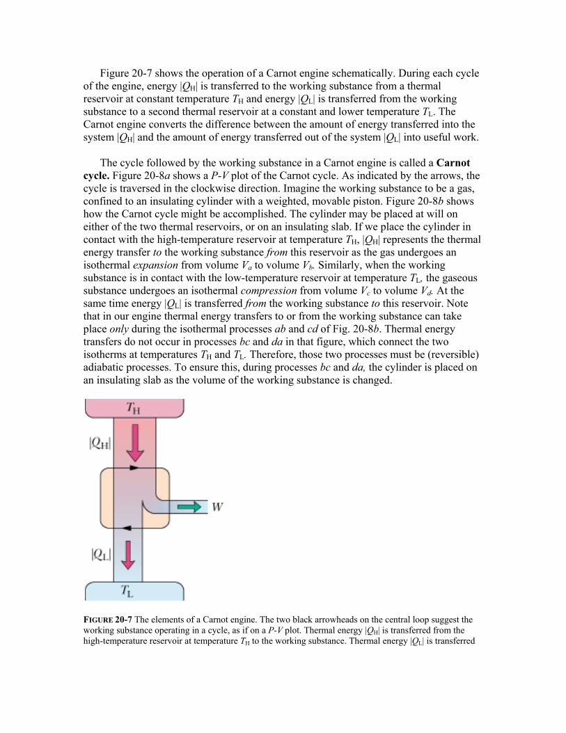
Figure 20-7 shows the operation of a Carnot engine schematically. During each cycle of the engine, energy |QH| is transferred to the working substance from a thermal reservoir at constant temperature TH and energy |QL| is transferred from the working substance to a second thermal reservoir at a constant and lower temperature TL. The Carnot engine converts the difference between the amount of energy transferred into the system |QH| and the amount of energy transferred out of the system |QL| into useful work.
The cycle followed by the working substance in a Carnot engine is called a Carnot cycle. Figure 20-8a shows a P-V plot of the Carnot cycle. As indicated by the arrows, the cycle is traversed in the clockwise direction. Imagine the working substance to be a gas, confined to an insulating cylinder with a weighted, movable piston. Figure 20-8b shows how the Carnot cycle might be accomplished. The cylinder may be placed at will on either of the two thermal reservoirs, or on an insulating slab. If we place the cylinder in contact with the high-temperature reservoir at temperature TH, |QH| represents the thermal energy transfer to the working substance from this reservoir as the gas undergoes an isothermal expansion from volume Va to volume Vb. Similarly, when the working substance is in contact with the low-temperature reservoir at temperature TL, the gaseous substance undergoes an isothermal compression from volume Vc to volume Vd. At the same time energy |QL| is transferred from the working substance to this reservoir. Note that in our engine thermal energy transfers to or from the working substance can take place only during the isothermal processes ab and cd of Fig. 20-8b. Thermal energy transfers do not occur in processes bc and da in that figure, which connect the two isotherms at temperatures TH and TL. Therefore, those two processes must be (reversible) adiabatic processes. To ensure this, during processes bc and da, the cylinder is placed on an insulating slab as the volume of the working substance is changed.
FIGURE 20-7 The elements of a Carnot engine. The two black arrowheads on the central loop suggest the working substance operating in a cycle, as if on a P-V plot. Thermal energy |QH| is transferred from the high-temperature reservoir at temperature TH to the working substance. Thermal energy |QL| is transferred

from the working substance to the low-temperature reservoir at temperature TL. Work W is done by the engine (actually by the working substance) on something in the environment.
FIGURE 20-8 (a) A pressure-volume plot of the cycle followed by the working substance of the Carnot engine in Fig. 20-7. The cycle consists of two isothermal processes (ab and cd) and two adiabatic processes (bc and da). The shaded area enclosed by the cycle is equal to the work W per cycle done by the Carnot engine. (b) An example of how this set of cycles could be accomplished. The upward motions of a piston during processes ab and bc are accomplished by slowly removing weight from the piston. The downward motions of the piston during processes cd and da are accomplished by slowing adding weight to the piston.
Work Done: During the consecutive processes ab and bc of Fig. 20-8, the working substance is expanding and thus doing positive work as it raises the weighted piston. This work is represented in Fig. 20-8a by the area under curve abc. During the consecutive processes cd and da, the working substance is being compressed, which means that it is doing negative work on its environment (the environment is doing positive work on it). This work is represented by the area under curve cda. The net work per cycle, which is represented by W in Figs. 20-7 and 20-8a, is the difference between these two areas. It is a positive quantity equal to the area enclosed by cycle abcda in Fig. 20-8a. This work W is performed on some outside object. The engine might, for example, be used to lift a weight.
To calculate the net work done by a Carnot engine during a cycle, let us apply the first law of thermodynamics (ΔEint = Q − W), to the working substance of a Carnot engine. That substance must return again and again to any arbitrarily selected state in that cycle. Thus, if X represents any state property of the working substance, such as pressure, temperature, volume, internal energy, or entropy, we must have ΔX = 0 for every cycle. It follows that ΔEint = 0 for a complete cycle of the working substance. Recall that Q in Eq.

19-18 is the net thermal energy transfer per cycle and W is the net work. We can then write the first law of thermodynamics (ΔEint = Q − W) for the Carnot cycle as
H L| | | | . (20-6)W Q Q
Entropy Changes: Equation 20-1 (ΔS = ∫dQ/T) tells us that any thermal energy transfer between a system and its surroundings must involve a change in entropy. To illustrate the entropy changes for a Carnot engine, we can plot the Carnot cycle on a temperature–entropy (T-S) diagram as in Fig. 20-9. The lettered points a, b, c, and d in Fig. 20-9 correspond to the lettered points in the P-V diagram in Fig. 20-8. The two horizontal lines in Fig. 20-9 correspond to the two isothermal processes of the Carnot cycle (because the temperature is constant). Process ab is the isothermal expansion stroke of the cycle. As the high temperature reservoir transfers thermal energy |QH| reversibly to the working substance at temperature TH, its entropy increases. Similarly, during the isothermal compression cd, the working substance transfers thermal energy |QL| reversibly to the low temperature reservoir at temperature TL. In this process the entropy of the working substance decreases.
FIGURE 20-9 The Carnot cycle of Fig. 20-8 plotted on a temperature–entropy diagram. During processes ab and cd the temperature remains constant. During processes bc and da the entropy remains constant.
The two vertical lines in Fig. 20-9 correspond to the two adiabatic processes of the Carnot cycle. Because no thermal energy transfers occur during the adiabatic processes, the entropy of the working substance does not change during either of these processes. So, in a Carnot engine, there are two (and only two) reversible thermal energy transfers, and thus two changes in entropy—one at temperature TH and one at TL. The net entropy change per cycle is then
H LH L
H L
| | | |. (20-7)
Q QS S S
T T

Here ΔSH is positive because energy |QH| is transferred to the working substance from the surroundings (an increase in entropy) and ΔSL is negative because energy |QL| is transferred from the working substance to the surroundings (a decrease in entropy). Because entropy is a state property, we must have ΔS = 0 for a complete cycle. Putting ΔS = 0 in above (Eq. 20-7) requires that
H L
H L
| | | |. (20-8)
Q Q
T T
Note that, because TH > TL, we must have H L| | | | .Q Q That is, more energy is transferred from the high-temperature reservoir to the engine than the engine transfers to the low-temperature reservoir.
We shall now use our findings on the work done (Eq. 20-6) and entropy change (Eq. 20-8) in an ideal Carnot cycle to derive an expression for the efficiency of an ideal Carnot engine.
Efficiency of an Ideal Carnot Engine
The purpose of any heat engine is to transform as much of the thermal energy, QH, transferred to the engine’s working medium into useful mechanical work as possible. We measure its success in doing so by its thermal efficiency ε, defined as the work the engine does per cycle (“energy we get”) divided by the thermal energy transferred to it per cycle (“energy we pay for”):
H
energy we get | | (efficiency, any engine). (20-9)
energy we pay for | |
W
Q
For a Carnot engine we can substitute W = |QH| − |QL| from Eq. 20-6 to writ
H L L
H H
1 . (20-10)C
Q Q Q
Q Q
Using |QH|/TH = |QL|/TL (Eq. 20-8) we can write this as
L
H
1 (efficiency, idea Carnot engine), (20-11)CT
T
where the temperatures TL and TH are in kelvin. Because TL < TH, the Carnot engine necessarily has a thermal efficiency less than unity—that is, less than 100%. This is indicated in Fig. 20-7, which shows that only part of the energy transferred to the engine from the high-temperature reservoir causes the engine’s working substance to expand and do physical work on the surroundings. The rest of the energy absorbed by the engine provides for the heat transfer to the low-temperature reservoir. We will show in Section

20-6 that no real engine can have a thermal efficiency greater than that calculated for the ideal Carnot engine (Eq. 20-11).
Other Types of Cycles and Real Engines
Efficiency is typically our main concern when designing an engine. For an engine that operates on an ideal Carnot cycle, the efficiency is
L
H
1 .CT
T
But remember, an ideal Carnot cycle means that the cycle is composed of the following four processes: a perfectly isothermal (constant temperature) expansion of the working substance, a perfectly adiabatic (zero thermal energy transfer) expansion of the working substance, a perfectly isothermal compression of the working substance, and a perfectly adiabatic compression of the working substance. Perfectly isothermal means the temperature of the working substance cannot change at all during these strokes. Perfectly adiabatic means that there can be no thermal energy transfer at all. These tasks are not easy to accomplish. If you do accomplish them, then you have an ideal Carnot cycle and the efficiency of the engine is given by the equation above. Most engines built on the Carnot cycle have efficiencies that are measurably lower than this.
It is important to note that even an ideal Carnot engine cannot have an efficiency of one. That is, it does not do a perfect job of converting thermal energy transferred to it into work. Inspection of the Carnot efficiency expression εC = 1 − TL/TH (Eq. 20-11) shows that we can achieve 100% engine efficiency (that is, ε = 1) only if TL = 0 K or TH → ∞. These requirements are impossible to meet. So, decades of practical engineering experience have led to the following alternative version of the second law of thermodynamics:
It is impossible to design an engine that converts thermal energy transferred to it from a thermal reservoir to useful work with 100% efficiency.
As we mentioned earlier, Carnot engines are not the only type of heat engine in which the working substance cycles between two constant temperatures and converts some of the associated heat transferred to the engine’s working medium to useful work. For example, Fig. 20-10 shows the operating cycle of an ideal Stirling engine. Comparison with the Carnot cycle of Fig. 20-8 shows that each cycle includes isothermal energy transfers at temperatures TH and TL. However, the two isotherms of the Stirling engine cycle of Fig. 20-10 are connected, not by adiabatic processes (no thermal energy transfer) as for the Carnot engine, but by constant-volume processes. To reversibly increase the temperature of a gas at constant volume from TL to TH (as in process da of Fig. 20-10) requires a thermal energy transfer to the working substance from a thermal reservoir whose temperature can be varied smoothly between those limits.

FIGURE 20-10 A P-V plot for the working substance of an ideal Stirling engine, assumed for convenience to be an ideal gas. Processes ab and cd are isothermal while bc and da are constant volume.
Note that reversible thermal energy transfers (and corresponding entropy changes) occur in all four of the processes that form the cycle of a Stirling engine, not just two processes as in a Carnot engine. Thus, the derivation that led to the efficiency expression for the Carnot engine (Eq. 20-11) does not apply to an ideal Stirling engine. More important, the efficiency of an ideal Stirling engine, or any other heat engine based on operation between two isotherms, is lower than that of a Carnot engine operating between the same two temperatures. This makes the ideal Carnot engine an ideal version of the ideal type of this class of engine! Of course, common Stirling engines have even lower efficiencies than the ideal Stirling engine discussed here.
Many engines important in our lives operate based on cycles between two isotherms and convert thermal energy transfers to work. For example, consider the nuclear power plant shown in Fig. 20-11. It, like most power plants, is an engine when taken in its entirety. A reactor core (or perhaps a coal-powered furnace) provides the high-temperature reservoir. Thermal energy transfer to the working substance (usually water) is converted to work done on a turbine (which often results in electricity production). The remaining energy |QL| is transferred to a low-temperature reservoir, which is usually a nearby river, or the atmosphere (if cooling towers are used). If the power plant shown in Fig. 20-11 operated as an ideal Carnot engine, its efficiency would be about 40%. Its actual efficiency is about 30%.

How does the efficiency of the internal combustion engine compare to that of the ideal Carnot engine? Well, this is a bit like comparing apples and oranges since the internal combustion engine does not operate between two isotherms like the Carnot, Stirling, or power plant engines do. However, we can estimate that if your car could be powered by a Carnot engine, it would have an efficiency of about 55% according to εC = 1 − TL/TH (Eq. 20-11). Its actual efficiency (with an internal combustion engine) is probably about 25%.
READING EXERCISE 20-4: Three Carnot engines operate between reservoir temperatures of (a) 400 and 500 K, (b) 600 and 800 K, and (c) 400 and 600 K. Rank the engines according to their thermal efficiencies, greatest first.
FIGURE 20 -11 The North Anna nuclear power plant near Charlottesville, Virginia, which generates electrical energy at the rate of 900 MW. At the same time, by design, it discards energy into the nearby river at the rate of 2000 MW. This plant—and all others like it—throws away more energy than it delivers in useful form. It is a real counterpart to the ideal engine of Fig. 20-7.
TOUCHSTONE EXAMPLE 20-3: Carnot Engine
Imagine an ideal Carnot engine that operates between the temperatures TH = 850 K and TL = 300 K. The engine performs 1200 J of work each cycle, the duration of each cycle being 0.25 s.
(a) What is the efficiency of this engine?
SOLUTION The Key Idea here is that the efficiency ε of an ideal Carnot engine depends only on the ratio TL/TH of the temperatures (in kelvins) of the thermal reservoirs to which it is connected. Thus, from Eq. 20-11, we have

L
H
300 K1 1 0.647 65% (Answer)
850 K
T
T
(b) What is the average power of this engine?
SOLUTION Here the Key Idea is that the average power P of an engine is the ratio of the work W it does per cycle to the time Δt that each cycle takes. For this Carnot engine, we find
1200 J4800 W 4.8 KW. (Answer)
0.25 s
WP
t
(c) How much thermal energy QH is extracted from the high-temperature reservoir every cycle?
SOLUTION Now the Key Idea is that, for any engine including a Carnot engine, the efficiency ε is the ratio of the work W that is done per cycle to the thermal energy QH that is extracted from the high-temperature reservoir per cycle. This relation, ε = |W|/|QH| (Eq. 20-9), gives us
H1200 J
1855 J. (Answer)0.647
WQ
(d) How much thermal energy QL is delivered to the low-temperature reservoir every cycle?
SOLUTION The Key Idea here is that for a Carnot engine, the work W done per cycle is equal to the difference in energy transfers |QH| − |QL|. (See Eq. 20-6.)Thus, we have
|QL| = |QH| − W = 1855 J − 1200 J = 655 J. (Answer)
(e) What entropy change is associated with the energy transfer to the working substance from the high-temperature reservoir? From the working substance to the low-temperature reservoir?
SOLUTION The Key Idea here is that the entropy change ΔS during a transfer of thermal energy Q at constant temperature T is given by Eq. 20-2 (ΔS = Q/T). Thus, for the transfer of energy QH from the high-temperature reservoir at TH, we have
HH
H
1855 J2.18 J/K
850 K
QS
T
For the transfer of energy QL to the low-temperature reservoir at TL, we have
LL
L
655 J2.18 J/K.
300 K
QS
T
Note that the algebraic signs of the two thermal energy transfers are different. Note also that, as Eq. 20-8 requires, the net entropy change of the working substance for one cycle (which is the algebraic sum of the two quantities calculated above) is zero.

TOUCHSTONE EXAMPLE 20-4: Better Than the Ideal?
An inventor claims to have constructed a heat engine that has an efficiency of 75% when operated between the boiling and freezing points of water. Is this possible?
SOLUTION The Key Idea here is that the efficiency of a real engine (with its irreversible processes and wasteful energy transfers) must be less than the efficiency of an ideal Carnot engine operating between the same two temperatures. From Eq. 20-11, we find that the efficiency of an ideal Carnot engine operating between the boiling and freezing points of water is
L
H
(0 273) K1 1
(100 273) K
0.268 27% (Answer)
T
T
Thus, the claimed efficiency of 75% for a real heat engine operating between the given temperatures is impossible.
20 -5 Entropy in the Real World: Refrigerators
A heat engine operated in a reverse cycle would require an input of work and transfer thermal energy from a low-temperature reservoir to a high-temperature reservoir as it continuously repeats a set series of thermodynamic processes. We call such a device a refrigerator. In a household refrigerator, for example, an electrical compressor does work in order to transfer thermal energy from the food storage compartment (a low-temperature reservoir) to the room (a high-temperature reservoir). Air conditioners and heat pumps are also refrigerators. The differences are only in the nature of the high- and low-temperature reservoirs. For an air conditioner, the low-temperature reservoir is the room that is to be cooled, and the high-temperature reservoir is the (presumably warmer) outdoors. A heat pump is an air conditioner that can also be operated in such a way as to transfer thermal energy to the air in a room from the (presumably cooler) outdoors.

FIGURE 20-12 The elements of a refrigerator. The two black arrowheads on the central loop suggest the working substance operating in a cycle, as if on a P-V plot. Thermal energy QL is transferred to the working substance from the low-temperature reservoir. Thermal energy QH is transferred to the high-temperature reservoir from the working substance. Work W is done on the refrigerator (on the working substance) by something in the environment.
Let us now consider an ideal refrigerator:
In an ideal refrigerator, all processes are reversible and no wasteful energy transfers occur between the refrigerator and its surroundings due to friction, turbulence, or other processes.
Figure 20-12 shows the basic elements of an ideal refrigerator that operates based on a Carnot cycle. That is, it is the Carnot engine of Fig. 20-8 operating in reverse. All the energy transfers, either thermal energy or work, are reversed from those of a Carnot engine. Thus, we call such an ideal refrigerator an ideal Carnot refrigerator.
The designer of a refrigerator would like to do amount of work W (that we pay for) and cause as large a thermal energy transfer |QL| as possible from the low-temperature reservoir (for example, the storage space in a kitchen refrigerator or the room to be cooled by the air conditioner). A measure of the efficiency of a refrigerator, then, is
Lwhat we want (coefficient of performance, any refrigerator), (20-12)
what we pay for
QK
W
where K is called the coefficient of performance. For a Carnot refrigerator, the first law of thermodynamics gives |W| = |QH| − |QL|, where |QH| is the amount of the thermal energy transfer to the high-temperature reservoir. The coefficient of performance for our ideal Carnot refrigerator then becomes
L
H L
. (20-13)C
QK
Q Q
Because an ideal Carnot refrigerator is an ideal Carnot engine operating in reverse, we can again use |QH|/TH = |QL|/TL (Eq. 20-8) and rewrite this expression as
L
H L
(coefficient of performance, Carnot refrigerator). (20-14)CT
KT T
For typical room air conditioners, K ≈ 2.5. For household refrigerators, K ≈ 5. Unfortunately, but logically, the efficiency (and so the value of K) of a given refrigerator is higher the closer the temperatures of the two reservoirs are to each other. For example, a given Carnot air conditioner is more efficient on a warm day than when it is very hot outside.

It would be nice to own a refrigerator that did not require an input of work—that is, one that would run without being plugged in. Figure 20-13 represents an “inventor’s dream,” of a perfect refrigerator that transfers thermal energy Q from a cold reservoir to a warm reservoir without the need for work. Because the unit returns to the same state at the end of each cycle, and entropy is a state property, we know that the change in entropy of the working substance for this imagined refrigerator would be zero for a complete cycle. The entropies of the two reservoirs, however, would change. The entropy change for the low temperature reservoir would be −|Q|/TL, and that for the high temperature reservoir would be +|Q|/TH. Thus, the net entropy change for the entire system is
L H
| | | |.
Q QS
T T
Because TH > TL, the right side of this equation would be negative and thus the net change in entropy per cycle for the closed system refrigerator + reservoirs would also be negative. Because such a decrease in entropy violates the second law of thermodynamics ΔS ≥ 0 (Eq. 20-5), it must be that a perfect refrigerator cannot exist. That is, if you want your refrigerator to operate, you must plug it in!
This result leads us to another (equivalent) formulation of the second law of thermodynamics:
It is impossible to design a refrigerator that can cause a thermal energy transfer from a reservoir at a lower temperature to one at a higher temperature without the input of work (that is, with 100% efficiency).
In short, there are no perfect refrigerators.
FIGURE 20-13 The elements of a perfect (but impossible) refrigerator—that is, one that transfers energy from a low-temperature reservoir to a high-temperature reservoir without any input of work.

READING EXERCISE 20-5: You wish to increase the coefficient of performance of an ideal Carnot refrigerator. You can do so by (a) running the cold chamber at a slightly higher temperature, (b) running the cold chamber at a slightly lower temperature, (c) moving the unit to a slightly warmer room, or (d) moving it to a slightly cooler room. Assume that the proposed changes in the magnitude of either TL of TH are the same in all four cases. List the changes according to the resulting coefficients of performance, greatest first.
20-6 Efficiency Limits of Real Engines
As we have just seen, a “perfect” Carnot refrigerator would violate the second law of thermodynamics which states that entropy must always either remain constant or increase. Therefore, we accept that a search for a 100% efficient Carnot refrigerator is futile. They do not exist. But what about Carnot engines? Can we have a “perfect” (that is, 100% efficient) engine?
Fundamentally, the inefficiency in an ideal Carnot engine is associated with the thermal energy transfer at the low temperature reservoir interface. Naive inventors continually try to improve Carnot engine efficiency by reducing the waste energy |QL| transferred to the low-temperature reservoir and, hence, “thrown away” during each cycle. The inventor’s dream is to produce the perfect engine, diagrammed in Fig. 20-14, in which |QL| is reduced to zero and |QH| is converted completely into work. For example, if we could do it, a perfect engine on an ocean liner could use thermal energy transferred to it from seawater to drive the propellers, with no fuel cost. An automobile, fitted with such a perfect engine, could use energy transferred from the surrounding air to turn its wheels, again with no fuel cost.
FIGURE 20-14 The elements of a perfect (and impossible) engine—that is, one that converts thermal energy transfer QH from a high-temperature reservoir directly to work W with 100% efficiency.

Alas, what seems too good to be true usually is. A perfect engine cannot exist. We already noted in Section 20-4 that since the efficiency of an ideal Carnot engine is given by εC = 1 − TL/TH (Eq. 20-11), even an ideal Carnot engine cannot have 100% efficiency. This is clear since we cannot have TL = 0 K or TH → ∞. So, if a real engine is to have 100% efficiency, it will have to have a higher efficiency than our ideal Carnot engine. Let’s see if that is possible.
Let us assume for a moment that an inventor, working in her garage, has constructed an engine X, which she claims has an efficiency εX that is greater than εC, where εC is the efficiency of an ideal Carnot engine operating between two temperatures. Then,
(a claim). (21-15)X C
FIGURE 20-15 (a) Engine X drives a Carnot refrigerator. (b) If, as claimed, engine X is more efficient than a Carnot engine, then the combination shown in (a) is equivalent to the perfect refrigerator shown here. This violates the second law of thermodynamics, so we conclude that engine X cannot be more efficient than a Carnot engine.
Let us connect the inventor’s engine X to a Carnot refrigerator, as in Fig. 20-15a. We adjust the strokes of the refrigerator so that the work it requires per cycle is just equal to that provided by the engine X. Thus, no (external) work is needed for the operation of the combination engine + refrigerator of Fig. 20-15a, which we take as our system. Since the efficiency of an engine is ε = energy we get/energy we pay for = |W|/|QH| (Eq. 20-9), and
,X C we must have

'HH
,W W
where 'HQ is the heat transfer at the high-temperature reservoir in engine X. The right side
of the inequality is the efficiency of the Carnot refrigerator shown in Fig. 20-15a when it operates (in reverse) as an engine. Since |W| is the same in both cases, this inequality requires that
'H H . (20-16)Q Q
Because the work done by engine X is equal to the work done on the Carnot refrigerator, which is (from Eq. 20-6) W = |QH| − |QL|, we have
' 'H L H L .Q Q Q Q
We can rearrange terms and write this as
H L
' 'H L . (20-17)Q Q Q Q Q
Here 'LQ is the thermal energy transfer at the low-temperature reservoir in engine X.
Because we found that 'H HQ Q (Eq. 20-16), the quantity Q must be positive. What
does Q represent? Careful evaluation of this expression (Eq. 20-17) tells us that Q is the net thermal energy transfer at the high-temperature reservoir as a result of our combined engine plus refrigerator. That is, the net effect of engine X and the Carnot refrigerator, working in combination, is to transfer thermal energy Q from a low-temperature reservoir to a high-temperature reservoir. Notably, this is done with no work input to the combined engine-refrigerator system. Thus, the combination acts like the perfect refrigerator of Fig. 20-13, whose existence is a violation of the second law of thermodynamics.
Thus, we conclude that engine X cannot be more efficient than the ideal Carnot engine. In general, no real engine can have an efficiency greater than that of a Carnot engine when both engines work between the same two temperatures. At most, it can have an efficiency equal to that of an ideal Carnot engine. In that case, engine X is an ideal Carnot engine. Since ideal Carnot engines cannot be 100% efficient, this means that “perfect” (100% efficient) engines are physically impossible.
20-7 A Statistical View of Entropy
In Chapter 20 we saw that the macroscopic properties of gases can be explained in terms of their microscopic, or molecular, behavior. For one example, recall that we were able to

account for the pressure exerted by a gas on the walls of its container in terms of the momentum transferred to those walls by rebounding gas molecules. Such explanations are part of a study called statistical mechanics.
Here we shall focus our attention on a single problem, involving the distribution of gas molecules between the two halves of an insulated box. This problem is reasonably simple to analyze, and it allows us to use statistical mechanics to calculate the entropy change for the free expansion of an ideal gas. You will see in Touchstone Example 20-6 that statistical mechanics leads to the same entropy change we obtain in Example 20-2 using thermodynamics.
Figure 20-16 shows a box that contains six identical (and thus indistinguishable) molecules of a gas. At any instant, a given molecule will be in either the left or the right half of the box; because the two halves have equal volumes, the molecule has the same likelihood, or probability, of being in either half.
FIGURE 20-16 An insulated box contains six gas molecules. Each molecule has the same probability of being in the left half of the box as in the right half. The arrangement in (a) corresponds to configuration III in Table 20-1, and that in (b) corresponds to configuration IV.
Table 20-1 shows four of the seven possible configurations of the six molecules, each configuration labeled with Roman numerals. For example, in configuration I, all six

molecules are in the left half of the box (n1 = 6, and none are in the right half (n2 = 0). The three configurations not shown are V with a (2, 4) split, VI with a (1, 5) split, and VII with a (0, 6) split. In configuration II, five molecules are in one half of the box, leaving one molecule in the other half. We see that, in general, a given configuration can be achieved in a number of different ways. We call these different arrangements of the molecules microstates. Let us see how to calculate the number of microstates that correspond to a given configuration.
TABLE 20-1 Six Molecules in a Box
Configurationa Multiplicity W (number of microstates)
Calculation of W (Eq. 20-18)
Entropy 10−23 J/K (Eq. 20-19) Label n1 n2
I 6 0 1 6!/(6! 0!) = 1 0
II 5 1 6 6!/(5! 1!) = 6 2.47
III 4 2 15 6!/(4! 2!) = 15 3.74
IV 3 3 20 6!/(3! 3!) = 20 4.13
Total number of microstates = 64
aThe configurations not listed are n1 = 0, n2 = 6; n1 = 1, n2 = 5; and n1 = 2, n2 = 4. These have the same multiplicities as I, II and III respectively.
Suppose we have N molecules, distributed with n1 molecules in one half of the box and n2 in the other half. (Thus n1 + n2 = N.) Let us imagine that we distribute the molecules “by hand,” one at a time. If N = 6, we can select the first molecule in six independent ways; that is, we can pick any one of the six molecules. We can pick the second molecule in five ways, by picking any one of the remaining five molecules, and so on. The total number of ways in which we can select all six molecules is the product of these independent ways, or 6 × 5 × 4 × 3 × 2 × 1 = 720. In mathematical shorthand we write this product as 6! = 720, where 6! is pronounced “six factorial.” Your hand-held calculator can probably calculate factorials. For later use you will need to know that 0! = 1. (Check this on your calculator.)
However, because the molecules are indistinguishable, these 720 arrangements are not all different. In the case that n1 = 4 and n2 = 2 (which is configuration III in Table 20-1), for example, the order in which you put four molecules in one half of the box does not matter, because after you have put all four in, there is no way that you can tell the order in which you did so. The number of ways in which you can order the four molecules is 4! or 24. Similarly, the number of ways in which you can order two molecules for the other half of the box is simply 2! or 2. To get the number of different arrangements that lead to the 4,2 split of configuration III, we must divide 720 by 24 and also by 2. We call the resulting quantity, which is the number of microstates that correspond to a given configuration, the multiplicity W of that configuration. Thus, for configuration III,

III6! 720
15.4!2! 24 2
W
Thus, Table 20-1 tells us there are 15 independent microstates that correspond to configuration III. Note that, as the table also tells us, the total number of microstates for six molecules distributed over four configurations is 42.
Extrapolating from six molecules to the general case of N molecules, we have
1 2
! (multiplicity of configuration). (20-18)
! !
NW
n n
You should verify that Eq. 20-18 gives the multiplicities for all the configurations listed in Table 20-1.
The basic assumption of statistical mechanics is:
All microstates are equally probable.
In other words, if we were to take a great many snapshots of the six molecules as they jostle around in the box of Fig. 20-16 and then count the number of times each microstate occurred, we would find that all 42 microstates will occur equally often. In other words, the system will spend, on average, the same amount of time in each of the 42 microstates listed in Table 20-1.
Because the microstates are equally probable, but different configurations have different numbers of microstates, the configurations are not equally probable. In Table 20-1 configuration IV, with 20 microstates, is the most probable configuration, with a probability of 20/64 = 0.313. This means that the system is in configuration IV 31.3% of the time. Configurations I and VII, in which all the molecules are in one half of the box, are the least probable, each with a probability of or 1/64 = 0.016 or 1.6%. It is not surprising that the most probable configuration is the one in which the molecules are evenly divided between the two halves of the box, because that is what we expect at thermal equilibrium. However, it is surprising that there is any probability, however small, of finding all six molecules clustered in half of the box, with the other half empty. In Touchstone Example 20-5 we show that this state can occur because six molecules is an extremely small number.
For large values of N there are extremely large numbers of microstates, but nearly all the microstates belong to the configuration in which the molecules are divided equally between the two halves of the box, as Fig. 20-17 indicates. Even though the measured temperature and pressure of the gas remain constant, the gas is churning away endlessly as its molecules “visit” all probable microstates with equal probability. However, because so few microstates lie outside the very narrow central configuration peak of Fig. 20-17,

we might as well assume that the gas molecules are always divided equally between the two halves of the box. As we shall see, this is the configuration with the greatest entropy.
FIGURE 20-17 For a large number of molecules in a box, a plot of the number of microstates that require various percentages of the molecules to be in the left half of the box. Nearly all the microstates correspond to an approximately equal sharing of the molecules between the two halves of the box; those microstates form the central configuration peak on the plot. For N ≈ 1022 molecules, the central configuration peak is much too narrow to be drawn on this plot.
Probability and Entropy
In 1877, Austrian physicist Ludwig Boltzmann (the Boltzmann of Boltzmann’s constant kB) derived a relationship between the entropy S of a configuration of a gas and the multiplicity W of that configuration. That relationship is
ln (Boltzmann's entropy equation). (20-19)BS k W
This famous formula is engraved on Boltzmann’s tombstone.
It is natural that S and W should be related by a logarithmic function. The total entropy of two systems is the sum of their separate entropies. The probability of occurrence of two independent systems is the product of their separate probabilities. Because ln ab = ln a + ln b, the logarithm seems the logical way to connect these quantities.
Table 20-1 displays the entropies of the configurations of the six-molecule system of Fig. 20-16, computed using Eq. 20-19. Configuration IV, which has the greatest multiplicity, also has the greatest entropy.
When you use Eq. 20-18 to calculate W, your calculator may signal “OVERFLOW” if you try to find the factorial of a number greater than a few hundred. Fortunately, there is a very good approximation, known as Stirling’s approximation, not for N! but for ln

N!, which as it happens is exactly what is needed in Eq. 20-19. Stirling’s approximation is
ln ! (ln ) (Stirling's approximation). (20-20)N N N N
The Stirling of this approximation is not the Stirling of the Stirling engine.
READING EXERCISE 20-6: A box contains one mole of a gas. Consider two configurations: (a) each half of the box contains one-half of the molecules, and (b) each third of the box contains one-third of the molecules. Which configuration has more microstates?
TOUCHSTONE EXAMPLE 20-5: Indistinguishable
Suppose that there are 100 indistinguishable molecules in the box of Fig. 20-16. How many microstates are associated with the configuration n1 = 50 and n2 = 50? How many are associated with the configuration n1 = 100 and n2 = 0? Interpret the results in terms of the relative probabilities of the two configurations.
SOLUTION The Key Idea here is that the multiplicity W of a configuration of indistinguishable molecules in a closed box is the number of independent microstates with that configuration, as given by Eq. 20-18. For the (n1, n2) configuration (50,50), that equation yields
1 2
157
64 64
29
! 100!
! ! 50!50!
9.33 10 (Answer)
(3.04 10 )(3.04 10 )
1.01 10 .
NW
n n
Similarly, for the configuration of (100, 0), we have
1 2
! 100! 1 11 (Answer)
! ! 100!0! 0! 1
NW
n n
Thus, a 50-50 distribution is more likely than a 100-0 distribution by the enormous factor of about 1 × 1029. If you could count, at one per nanosecond, the number of microstates that correspond to the 50-50 distribution, it would take you about 3 × 10¹² years, which is about 750 times longer than the age of the universe. Even 100 molecules is still a very small number. Imagine what these calculated probabilities would be like for a mole of molecules—say, about N = 1024. You need never worry about suddenly finding all the air molecules clustering in one corner of your room!

TOUCHSTONE EXAMPLE 20-6: Entropy Increase
In Touchstone Example 20-1 we showed that when n moles of an ideal gas doubles its volume in a free expansion, the entropy increase from the initial state i to the final state f is Sf − Si = nR ln 2. Derive this result with statistical mechanics.
SOLUTION One Key Idea here is that we can relate the entropy S of any given configuration of the molecules in the gas to the multiplicity W of microstates for that configuration, using Eq. 20-19 (S = kB ln W). We are interested in two configurations: the final configuration f (with the molecules occupying the full volume of their container in Fig. 20-1b) and the initial configuration i (with the molecules occupying the left half of the container).
A second Key Idea is that, because the molecules are in a closed container, we can calculate the multiplicity W of their microstates with Eq. 20-18. Here we have N molecules in the n moles of the gas. Initially, with the molecules all in the left half of the container, their (n1, n2) configuration is (N, 0). Then, Eq. 20-18 gives their multiplicity as
!1.
!0!i
NW
N
Finally, with the molecules spread through the full volume, their (n1, n2) configuration is (N/2, N/2). Then, Eq. 20-18 gives their multiplicity as
!.
( /2)!( /2)!f
NW
N N
From Eq. 20-19, the initial and final entropies are
Si = k ln Wi = k ln 1 = 0
and
ln ln( !) 2 ln[( /2)!]. (20 - 21)f B f BS k W k N k N
In writing Eq. 20-21, we have used the relation
2ln ln 2ln .
aa b
b
Now, applying Eq. 20-20 to evaluate Eq. 20-21, we find that
ln( !) 2 ln[( /2)!]
[ (ln ) ] 2 [( /2) ln ( /2) ( /2)]
[ (ln ) ln ( /2) ] (20 - 22)
[ (ln ) (ln ln 2)] ln 2.
B B
B B
B
B B
Sf k N k N
k N N N k N N N
k N N N N N N
k N N N N Nk
From Eq. 20-7 we can substitute nR for NkB, where R is the universal gas constant. Equation 20-22 then becomes
l n 2.fS nR

The change in entropy from the initial state to the final is thus
ln 2 0
ln 2, (Answer)
f iS S nR
nR
which is what we set out to show. In Touchstone Example 20-1 we calculated this entropy increase for a free expansion with thermodynamics by finding an equivalent reversible process and calculating the entropy change for that process in terms of temperature and heat transfer. Here we have calculated the same increase with statistical mechanics using the fact that the system consists of molecules.

Conceptual Questions
1 Point i in Fig. 20-19 represents the initial state of an ideal gas at temperature T. Taking algebraic signs into account, rank the entropy changes that the gas undergoes as it moves, successively and reversibly, from point i to points a, b, c, and d, greatest first.
Figure 20-19 Question 1.
2 In four experiments, blocks A and B, starting at different initial temperatures, were brought together in an insulating box and allowed to reach a common final temperature. The entropy changes for the blocks in the four experiments had the following values (in joules per kelvin), but not necessarily in the order given. Determine which values for A go with which values for B.
Block Values
A 8 5 3 9
B -3 -8 -5 -2
3 A gas, confined to an insulated cylinder, is compressed adiabatically to half its volume. Does the entropy of the gas increase, decrease, or remain unchanged during this process?
4 An ideal monatomic gas at initial temperature T0 (in kelvins) expands from initial volume V0 to volume 2V0 by each of the five processes indicated in the T-V diagram of Fig. 20-20. In which process is the expansion (a) isothermal, (b) isobaric (constant pressure), and (c) adiabatic? Explain your answers. (d) In which processes does the entropy of the gas decrease?

Figure 20-20 Question 4.
5 In four experiments, 2.5 mol of hydrogen gas undergoes reversible isothermal expansions, starting from the same volume but at different temperatures. The corresponding p-V plots are shown in Fig. 20-21. Rank the situations according to the change in the entropy of the gas, greatest first.
Figure 20-21 Question 5.
6 A box contains 100 atoms in a configuration that has 50 atoms in each half of the box. Suppose that you could count the different microstates associated with this configuration at the rate of 100 billion states per second, using a supercomputer. Without written calculation, guess how much computing time you would need: a day, a year, or much more than a year.
7 Does the entropy per cycle increase, decrease, or remain the same for (a) a Carnot engine, (b) a real engine, and (c) a perfect engine (which is, of course, impossible to build)?
8 Three Carnot engines operate between temperature limits of (a) 400 and 500 K, (b) 500 and 600 K, and (c) 400 and 600 K. Each engine extracts the same amount of energy per cycle from the high-temperature reservoir. Rank the magnitudes of the work done by the engines per cycle, greatest first.
9 An inventor claims to have invented four engines, each of which operates between constant-temperature reservoirs at 400 and 300 K. Data on each engine, per cycle of operation, are: engine A, QH = 200 J, QL = -175 J, and W = 40 J; engine B, QH = 500 J, QL = -200 J, and W = 400 J; engine C, QH = 600 J, QL = -200 J, and W = 400 J; engine D, QH = 100 J, QL = -90 J, and W = 10 J. Of the first and second laws of thermodynamics, which (if either) does each engine violate?
10 Does the entropy per cycle increase, decrease, or remain the same for (a) a Carnot refrigerator, (b) a real refrigerator, and (c) a perfect refrigerator (which is, of course, impossible to build)?
Problems
SEC. 20-2 CHANGE IN ENTROPY
1. Expands Reversibly A 2.50 mol sample of an ideal gas expands reversibly and isothermally at 360 K until its volume is doubled. What is the increase in entropy of the gas?
2. Reversible Isothermal How much thermal energy must be transferred for a reversible isothermal expansion of an ideal gas at 132 °C if the entropy of the gas increases by 46.0 J/K?
3. Four Moles Four moles of an ideal gas undergo a reversible isothermal expansion from volume V1 to volume V2 = 2V1 at temperature T = 400 K. Find (a) the work done by the gas and (b) the entropy change of the gas. (c) If the expansion is reversible and adiabatic instead of isothermal, what is the entropy change of the gas?
4. Reversible Isothermal Expansion An ideal gas undergoes a reversible isothermal expansion at 77.0°C, increasing its volume from 1.30 L to 3.40 L. The entropy change of the gas is 22.0 J/K. How many moles of gas are present?
5. Energy Absorbed Find (a) the thermal energy transfer and (b) the change in entropy of a 2.00 kg block of copper whose temperature is increased reversibly from 25°C to 100°C. The specific heat of copper is 386 J/kg K.
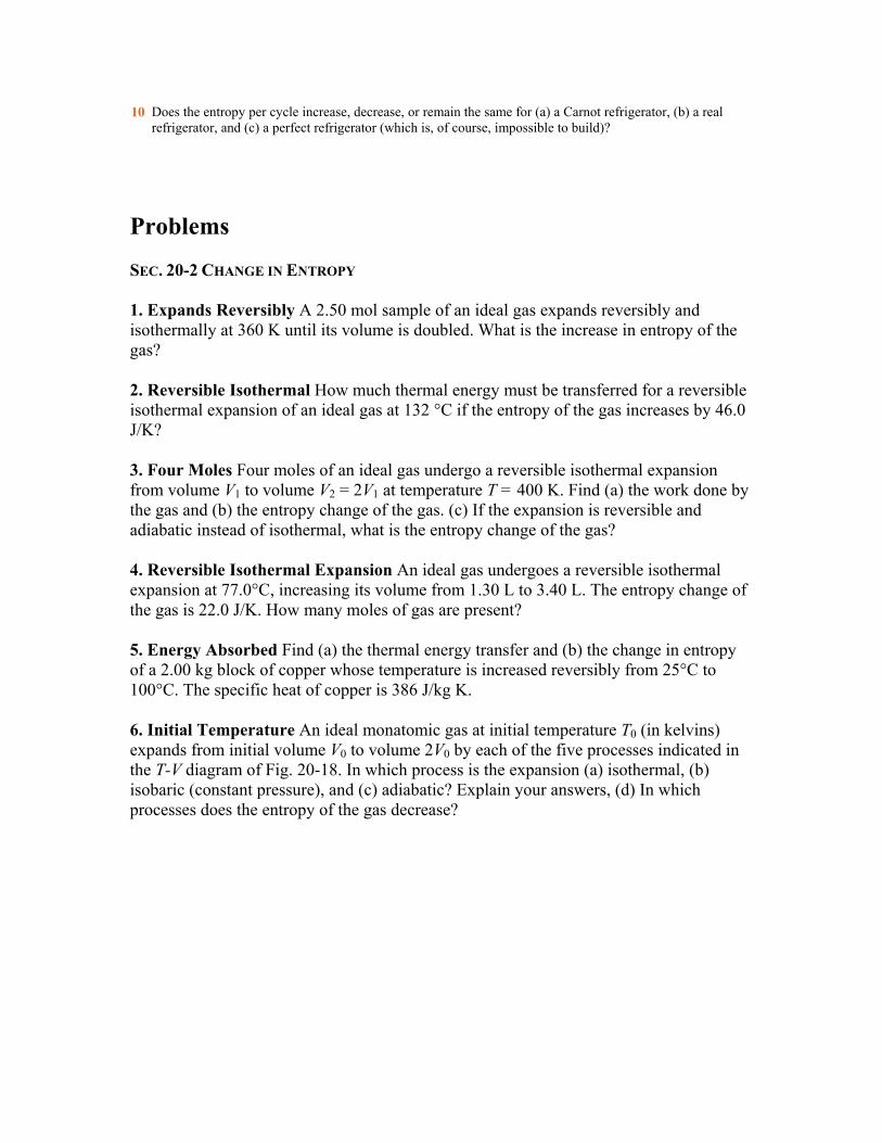
6. Initial Temperature An ideal monatomic gas at initial temperature T0 (in kelvins) expands from initial volume V0 to volume 2V0 by each of the five processes indicated in the T-V diagram of Fig. 20-18. In which process is the expansion (a) isothermal, (b) isobaric (constant pressure), and (c) adiabatic? Explain your answers, (d) In which processes does the entropy of the gas decrease?

FIGURE 20-18 Problem 6.
7. Entropy Change (a) What is the entropy change of a 12.0 g ice cube that melts completely in a bucket of water whose temperature is just above the freezing point of water? (b) What is the entropy change of a 5.00 g spoonful of water that evaporates completely on a hot plate whose temperature is slightly above the boiling point of water?
8. Ideal Gas Undergoes A 2.0 mol sample of an ideal monatomic gas undergoes the reversible process shown in Fig. 20-19. (a) How much thermal energy is transferred to the gas? (b) What is the change in the internal energy of the gas? (c) How much work is done by the gas?
FIGURE 20-19 Problems 8.
9. Aluminum and Water In an experiment, 200 g of aluminum (with a specific heat of 900 J/kg-K) at 100°C is mixed with 50.0 g of water at 20.0°C, with the mixture thermally isolated. (a) What is the equilibrium temperature? What are the entropy changes of (b) the aluminum, (c) the water and (d) the aluminum–water system?
10. Irreversible Process In the irreversible process of Fig. 20-5, let the initial temperatures of identical blocks L and R be 305.5 K and 294.5 K, respectively. Let 215 J

be the thermal energy transfer between the blocks required to reach equilibrium. Then for the reversible processes of Fig. 20-6, what are the entropy changes of (a) block L, (b) its reservoir, (c) block R, (d) its reservoir, (e) the two-block system, and (f) the system of the two blocks and the two reservoirs?
11. Reversible Apparatus Use the reversible apparatus of Fig. 20-6 to show that, if the process of Fig. 20-5 happened in reverse, the entropy of the system would decrease, a violation of the second law of thermodynamics.
12. Rotating Not Oscillating An ideal diatomic gas, whose molecules are rotating but not oscillating, is taken through the cycle in Fig. 20-20. Determine for all three processes, in terms of P1, V1, T1, and R: (a) P2, P3, and T3 and (b) W, Q, ΔEint and ΔS per mole?
FIGURE 20-20 Problem 12.
13. Copper in Box A 50.0 g block of copper whose temperature is 400 K is placed in an insulating box with a 100 g block of lead whose temperature is 200 K. (a) What is the equilibrium temperature of the two-block system? (b) What is the change in the internal energy of the two-block system between the initial state and the equilibrium state? (c) What is the change in the entropy of the two-block system? (See Table 19-2.)
14. Initial to Final One mole of a monatomic ideal gas is taken from an initial pressure P and volume V to a final pressure 2P and volume 2V by two different processes: (I) It expands isothermally until its volume is doubled, and then its pressure is increased at constant volume to the final pressure. (II) It is compressed isothermally until its pressure is doubled, and then its volume is increased at constant pressure to the final volume. (a) Show the path of each process on a P-V diagram. For each process calculate, in terms of P and V, (b) the thermal energy absorbed by the gas in each part of the process, (c) the work done by the gas in each part of the process, (d) the change in internal energy of the gas, ΔEint, and (e) the change in entropy of the gas, ΔS.

15. Ice Cube in a Lake A 10 g ice cube at −10°C is placed in a lake whose temperature is 15°C. Calculate the change in entropy of the cube–lake system as the ice cube comes to thermal equilibrium with the lake. The specific heat of ice is 2220 J/kg · K. (Hint: Will the ice cube affect the temperature of the lake?)
16. Ice Cube in Thermos An 8.0 g ice cube at −10°C is put into a Thermos flask containing 100 cm3 of water at 20°C. By how much has the entropy of the cube–water system changed when a final equilibrium state is reached? The specific heat of ice is 2220 J/kg K.
17. Water and Ice A mixture of 1773 g of water and 227 g of ice is in an initial equilibrium state at 0.00°C. The mixture is then, in a reversible process, brought to a second equilibrium state where the water–ice ratio, by mass, is 1:1 at 0.00°C. (a) Calculate the entropy change of the system during this process. (The heat of fusion for water is 333 kJ/kg.) (b) The system is then returned to the initial equilibrium state in an irreversible process (say, by using a Bunsen burner). Calculate the entropy change of the system during this process. (c) Are your answers consistent with the second law of thermodynamics?
18. Cylinder of Gas A cylinder contains n moles of a monatomic ideal gas. If the gas undergoes a reversible isothermal expansion from initial volume Vi to final volume Vf along path I in Fig. 20-21, its change in entropy is ΔS = nR ln (Vf/Vi). (See Touchstone Example 20-1) Now consider path II in Fig. 20-21, which takes the gas from the same initial state i to state x by a reversible adiabatic expansion, and then from that state x to the same final state f by a reversible constant volume process. (a) Describe how you would carry out the two reversible processes for path II. (b) Show that the temperature of the gas in state x is
Tx = Ti(Vi/Vf)2/3.
(c) What are the thermal energy transferred along path I (QI) and the thermal energy transferred along path II (QII)? Are they equal? (d) What is the entropy change ΔS for path II? Is the entropy change for path I equal to it? (e) Evaluate Tx, QI, QII, and ΔS for n = 1, Ti = 500 K, and Vf/Vi = 2.

FIGURE 20-21 Problem 18.
19. Through the Cycle One mole of an ideal monatomic gas is taken through the cycle in Fig. 20-22. (a) How much work is done by the gas in going from state a to state c along path abc? What are the changes in internal energy and entropy in going (b) from b to c and (c) through one complete cycle? Express all answers in terms of the pressure P0, volume V0, and temperature T0 of state a.
FIGURE 20-22 Problem 19.
20. Initial Pressure and Temperature One mole of an ideal monatomic gas, at an initial pressure of 5.00 kPa and initial temperature of 600 K, expands from initial volume Vi = 1.00 m3 to final volume Vf = 2.00 m3. During the expansion, the pressure P and volume V of the gas are related by P = (5.00 kPa) exp[(Vi – V)/a], where a = 1.00 m3. What are (a) the final pressure and (b) the final temperature of the gas? (c) How much work is done by the gas during the expansion? (d) What is the change in entropy of the gas during the expansion? (Hint: Use two simple reversible processes to find the entropy change.)
SEC. 20-4 ENTROPY IN THE REAL WORLD: ENGINES
Consider all Carnot engines discussed in these problems to be ideal.

21. Work and Efficiency in a Cycle A Carnot engine absorbs 52 kJ of thermal energy and exhausts 36 kJ as thermal energy in each cycle. Calculate (a) the engine’s efficiency and (b) the work done per cycle in kilojoules.
22. Low-Temp Reservoir A Carnot engine whose low-temperature reservoir is at 17°C has an efficiency of 40%. By how much should the temperature of the high-temperature reservoir be increased to increase the efficiency to 50%?
23. Operates Between A Carnot engine operates between 235°C and 115°C, absorbing 6.30 × 10⁴ J per cycle at the higher temperature. (a) What is the efficiency of the engine? (b) How much work per cycle is this engine capable of performing?
24. Reactor In a hypothetical nuclear fusion reactor, the fuel is deuterium gas at temperature of about 7 × 10⁸ K. If this gas could be used to operate a Carnot engine with TL = 100°C, what would be the engine’s efficiency?
25. Carnot Engine A Carnot engine has an efficiency of 22.0%. It operates between constant-temperature reservoirs differing in temperature by 75.0°C. What are the temperatures of the two reservoirs?
26. Engine Has Power A Carnot engine has a power of 500 W. It operates between constant-temperature reservoirs at 100°C and 60.0°C. What are (a) the rate of thermal energy input and (b) the rate of exhaust heat output, in kilojoules per second?
27. Process bc One mole of a monatomic ideal gas is taken through the reversible cycle shown in Fig. 20-23. Process bc is an adiabatic expansion, with Pb = 10.0 atm and Vb = 1.00 × 10⁻³ m3. Find (a) the thermal energy transferred to the gas, (b) the thermal energy transferred from the gas, (c) the net work done by the gas, and (d) the efficiency of the cycle.
FIGURE 20-23 Problem 27.

28. Enclosed Area Show that the area enclosed by the Carnot cycle on the temperature–entropy plot of Fig. 20-9 represents the net thermal energy transfer per cycle to the working substance.
29. Assume P = 2P0 One mole of an ideal monatomic gas is taken through the cycle shown in Fig. 20-24. Assume that P = 2P0, V = 2V0, P0 = 1.01 × 10⁵ Pa, and V0 = 0.0225 m3. Calculate (a) the work done during the cycle, (b) the thermal energy added during stroke abc, and (c) the efficiency of the cycle. (d) What is the efficiency of a Carnot engine operating between the highest and lowest temperatures that occur in the cycle? How does this compare to the efficiency calculated in (c)?
FIGURE 20-24 Problem 29.
30. First Stage In the first stage of a two-stage Carnot engine, thermal energy Q1 is absorbed at temperature T1, work W1 is done, and thermal energy Q2 is expelled at a lower temperature T2. The second stage absorbs that energy Q2, does work W2, and expels energy Q3 at a still lower temperature T3. Prove that the efficiency of the two-stage engine is (T1 = T3)/T1.
31. Deep Shaft Suppose that a deep shaft were drilled in Earth’s crust near one of the poles, where the surface temperature is −40°C, to a depth where the temperature is 800°C. (a) What is the theoretical limit to the efficiency of an engine operating between these temperatures? (b) If all the thermal energy released as heat into the low-temperature reservoir were used to melt ice that was initially at −40°C, at what rate could liquid water at 0°C be produced by a 100 MW power plant (treat it as an engine)? The specific heat of ice is 2220 J/kg · K; water’s heat of fusion is 333 kJ/kg. (Note that the engine can operate only between 0°C and 800°C in this case. Energy exhausted at −40°C cannot be used to raise the temperature of anything above −40°C)
32. Working Substance One mole of an ideal gas is used as the working substance of an engine that operates on the cycle shown in Fig. 20-25. BC and DA are reversible adiabatic processes. (a) Is the gas monatomic, diatomic, or polyatomic? (b) What is the efficiency of the engine?

FIGURE 20-25 Problem 32.
33. Gasoline Engine The operation of a gasoline internal combustion engine is represented by the cycle in Fig. 20-26. Assume the gasoline-air intake mixture is an ideal gas and use a compression ratio of 4:1 (V4 = 4V1). Assume that P2 = 3P1. (a) Determine the pressure and temperature at each of the vertex points of the P-V diagram in terms of P1, T1, and the ratio γ of the molar specific heats of the gas. (b) What is the efficiency of the cycle?
FIGURE 20-26 Problem 33.
SEC. 20-5 ENTROPY IN THE REAL WORLD: REFRIGERATORS
34. Carnot Refrigerator A Carnot refrigerator does 200 J of work to remove 600 J of thermal energy from its cold compartment. (a) What is the refrigerator’s coefficient of performance? (b) How much thermal energy per cycle is exhausted to the kitchen?

35. Carnot Air Conditioner A Carnot air conditioner takes energy from the thermal energy of a room at 70°F and transfers it to the outdoors, which is at 96°F. For each joule of electric energy required to operate the air conditioner, how many joules are removed from the room?
36. Heat Pump Transfers The electric motor of a heat pump transfers thermal energy from the outdoors, which is at −5.0°C, to a room, which is at 17°C. If the heat pump were a Carnot heat pump (a Carnot engine working in reverse), how many joules would be transferred to the thermal energy of the room for each joule of electric energy consumed?
37. Heat Pump to Heat Building A heat pump is used to heat a building. The outside temperature is −5.0°C, and the temperature inside the building is to be maintained at 22°C. The pump’s coefficient of performance is 3.8, and the heat pump delivers 7.54 MJ of thermal energy to the building each hour. If the heat pump is a Carnot engine working in reverse, at what rate must work be done to run the heat pump?
38. How Much Work How much work must be done by a Carnot refrigerator to transfer 1.0 J of thermal energy (a) from a reservoir at 7.0°C to one at 27°C, (b) from a reservoir at −73°C to one at 27°C, (c) from a reservoir at −173°C to one at 27°C, and (d) from a reservoir at −223°C to one at 27°C?
39. Air Conditioner An air conditioner operating between 93°F and 70°F is rated at 4000 Btu/h cooling capacity. Its coefficient of performance is 27% of that of a Carnot refrigerator operating between the same two temperatures. What horsepower is required of the air conditioner motor?
40. Motor in Refrigerator The motor in a refrigerator has a power of 200 W If the freezing compartment is at 270 K and the outside air is at 300 K, and assuming the efficiency of a Carnot refrigerator, what is the maximum amount of thermal energy that can be extracted from the freezing compartment in 10.0 min?
41. Engine Driving Refrigerator A Carnot engine works between temperatures T1 and T2. It drives a Carnot refrigerator that works between temperatures T3 and T4 (Fig. 20-27). Find the ratio |Q3|/|Q1| in terms of T1, T2, T3, and T4.

FIGURE 20-27 Problem 41.
SEC. 20-7 A STATISTICAL VIEW OF ENTROPY
42. Construct a Table Construct a table like Table 20-1 for eight molecules.
43. Show for N Molecules Show that for N molecules in a box, the number of possible microstates is 2N when microstates are defined by whether a given molecule is in the left half of the box or the right half. Check this for the situation of Table 20-1.
44. A Box of N Gas Molecules A box contains N gas molecules, equally divided between its two halves. For N = 50: (a) What is the multiplicity of this central configuration? (b) What is the total number of microstates for the system? (Hint: See Problem 43.) (c) What percentage of the time does the system spend in its central configuration? (d) Repeat (a) through (c) for N = 100. (e) Repeat (a) through (c) for N = 200. (f) As N increases, you will find that the system spends less time (not more) in its central configuration. Explain why this is so.
45. Three Equal Parts A box contains N gas molecules. Consider the box to be divided into three equal parts. (a) By extension of Eq. 20-18, write an equation for the multiplicity of any given configuration, (b) Consider two configurations: configuration A with equal numbers of molecules in all three thirds of the box, and configuration B with equal numbers of molecules in both halves of the box. What is the ratio WA/WB of the multiplicity of configuration A to that of configuration B? (c) Evaluate WA/WB for N = 100. (Because 100 is not evenly divisible by 3, put 34 molecules into one of the three box parts and 33 in each of the other parts for configuration A.)
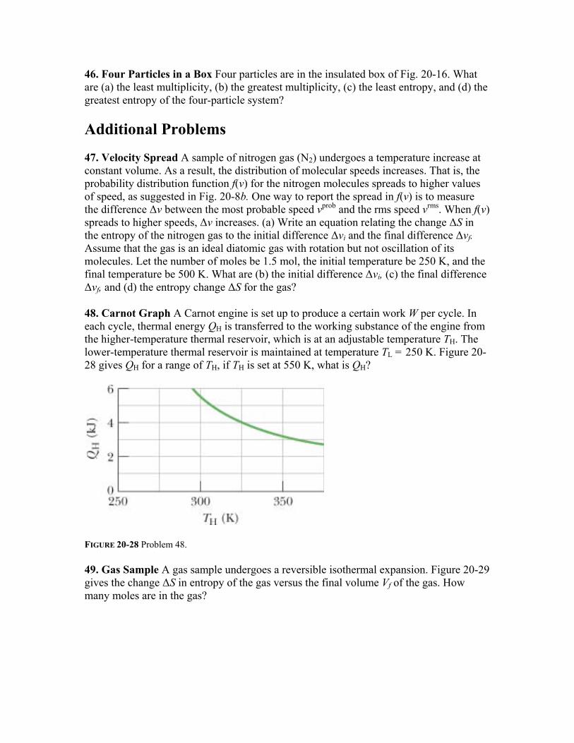
46. Four Particles in a Box Four particles are in the insulated box of Fig. 20-16. What are (a) the least multiplicity, (b) the greatest multiplicity, (c) the least entropy, and (d) the greatest entropy of the four-particle system?
Additional Problems
47. Velocity Spread A sample of nitrogen gas (N2) undergoes a temperature increase at constant volume. As a result, the distribution of molecular speeds increases. That is, the probability distribution function f(v) for the nitrogen molecules spreads to higher values of speed, as suggested in Fig. 20-8b. One way to report the spread in f(v) is to measure the difference Δv between the most probable speed vprob and the rms speed vrms. When f(v) spreads to higher speeds, Δv increases. (a) Write an equation relating the change ΔS in the entropy of the nitrogen gas to the initial difference Δvi and the final difference Δvf. Assume that the gas is an ideal diatomic gas with rotation but not oscillation of its molecules. Let the number of moles be 1.5 mol, the initial temperature be 250 K, and the final temperature be 500 K. What are (b) the initial difference Δvi, (c) the final difference Δvf, and (d) the entropy change ΔS for the gas?
48. Carnot Graph A Carnot engine is set up to produce a certain work W per cycle. In each cycle, thermal energy QH is transferred to the working substance of the engine from the higher-temperature thermal reservoir, which is at an adjustable temperature TH. The lower-temperature thermal reservoir is maintained at temperature TL = 250 K. Figure 20-28 gives QH for a range of TH, if TH is set at 550 K, what is QH?
FIGURE 20-28 Problem 48.
49. Gas Sample A gas sample undergoes a reversible isothermal expansion. Figure 20-29 gives the change ΔS in entropy of the gas versus the final volume Vf of the gas. How many moles are in the gas?
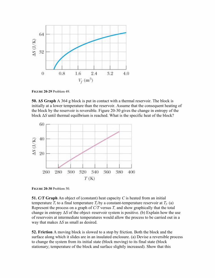
FIGURE 20-29 Problem 49.
50. ΔS Graph A 364 g block is put in contact with a thermal reservoir. The block is initially at a lower temperature than the reservoir. Assume that the consequent heating of the block by the reservoir is reversible. Figure 20-30 gives the change in entropy of the block ΔS until thermal equilbrium is reached. What is the specific heat of the block?
FIGURE 20-30 Problem 50.
51. C/T Graph An object of (constant) heat capacity C is heated from an initial temperature Ti to a final temperature Tf by a constant-temperature reservoir at Tf. (a) Represent the process on a graph of C/T versus T, and show graphically that the total change in entropy ΔS of the object–reservoir system is positive. (b) Explain how the use of reservoirs at intermediate temperatures would allow the process to be carried out in a way that makes ΔS as small as desired.
52. Friction A moving block is slowed to a stop by friction. Both the block and the surface along which it slides are in an insulated enclosure. (a) Devise a reversible process to change the system from its initial state (block moving) to its final state (block stationary; temperature of the block and surface slightly increased). Show that this

reversible process results in an entropy increase for the closed block–surface system. For the process, you can use an ideal engine and a constant-temperature reservoir. (b) Show, using the same process, but in reverse, that if the temperature of the system were to decrease spontaneously and the block were to start moving again, the entropy of the system would decrease (a violation of the second law of thermodynamics).
53. T-S Diagram A diatomic gas of 2 mol is taken reversibly around the cycle shown in the T-S diagram of Fig. 20-31. The molecules rotate but do not oscillate. What are the thermal energy transfers Q for (a) the path from point 1 to point 2, (b) the path from point 2 to point 3, and (c) the full cycle? (d) What is the work W for the isothermal process? The volume V1 at point 1 is 0.200 m3. What are the volumes at (e) point 2 and (f) point 3?
What are the changes ΔEint in internal energy for (g) the path from point 1 to point 2, (h) the path from point 2 to point 3, and (i) the full cycle? (Hint: Part (h) can be done with one or two lines of calculation using Section 20-8 or with a page of calculation using Section 20-11.) (j) What is the work W for the adiabatic process?
FIGURE 20-31 Problem 53.
54. Inventor’s Engine An inventor has built an engine (engine X) and claims that its efficiency εX is greater than the efficiency ε of an ideal engine operating between the same two temperatures. Suppose that you couple engine X to an ideal refrigerator (Fig. 20-32a) and adjust the cycle of engine X so that the work per cycle that it provides equals the work per cycle required by the ideal refrigerator. Treat this combination as a single unit and show that if the inventor’s claim were true (if εX > ε), the combined unit would act as a perfect refrigerator (Fig. 20-32b), transferring thermal energy from the low temperature reservoir to the high-temperature reservoir without the need of work.
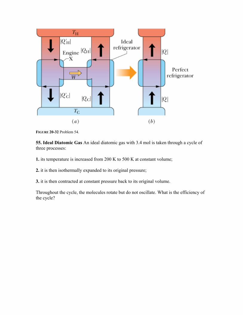
FIGURE 20-32 Problem 54.
55. Ideal Diatomic Gas An ideal diatomic gas with 3.4 mol is taken through a cycle of three processes:
1. its temperature is increased from 200 K to 500 K at constant volume;
2. it is then isothermally expanded to its original pressure;
3. it is then contracted at constant pressure back to its original volume.
Throughout the cycle, the molecules rotate but do not oscillate. What is the efficiency of the cycle?