
20, 1965 - suppes-corpus.stanford.edusuppes-corpus.stanford.edu/techreports/IMSSS_75.pdf ·...
88
A CORRELATED URN-SCHEME FOR A CONTINUUM OF RESPONSES By Barry Charles Arnold TECHNICAL REPORT NO. 75 July 20, 1965 PSYCHOLOGY SERIES Reproduction in Whole or in Part is Permitted for any Purpose of the United States Government INSTITUTE FOR· MATHEMATICAL STUDIES IN THE SOCIAL SCIENCES '. . . . STANFORD UNIVERSITY STANFORD, CALIFORNIA
-
Upload
duonghuong -
Category
Documents
-
view
214 -
download
0
Transcript of 20, 1965 - suppes-corpus.stanford.edusuppes-corpus.stanford.edu/techreports/IMSSS_75.pdf ·...

A CORRELATED URN-SCHEME FOR A CONTINUUM OF RESPONSES
By
Barry Charles Arnold
TECHNICAL REPORT NO. 75
July 20, 1965
PSYCHOLOGY SERIES
Reproduction in Whole or in Part is Permitted for
any Purpose of the United States Government
INSTITUTE FOR· MATHEMATICAL STUDIES IN THE SOCIAL SCIENCES'. . . .
STANFORD UNIVERSITY
STANFORD, CALIFORNIA


A CORRELATED URN-SCHEME FOR A CONTINUUM OF RESPONSES*
Barry Charles Arnold
INTRODUCTION
'rtis thesis is concerned with the analysis of a new model to cover
the case of simple learning with a continuum of responses and reinforce-
ments, Suppes (1959) suggested a generalization of the finite response
linear model to cover this case as well as analogous generalizations of
the pattern and component stimulus sampling models (1960), Some studies
of the empirical validity of these models have appeared in the literature
(e,g" Suppes and Rouanet (1964), Suppes, Rouanet, Levine and Frankmann
(1964», It is apparent from these studies that the above mentioned
models perform unsatisfactorily when predicting sequential probabilities
and the dependence of responses on recent reinforcements, This prompts
a search for alternative models, The model advocated and studied in
this thesis has been called a correlated urn-scheme, Although this
model appears to have numerOus parameters and regularity assumptions,
it will be seen that it leads to quite simple and tractable distribution
theory, It will also be seen that reasonably natural consistent estimates
of many of the parameters are obtainable, But a new model is only
*This research has been supported in part by the Air Force Office ofScientific Research under Contract AF49(638)-1253,
- 1 -

justifiable if it explains better empirically observed results. In
Appendix A will be found an empirical comparison of the correlated urn-
scheme with the linear and pattern models based on the data from Suppes,
Rouanet, Levine and Frankmann (1964).
- 2 -
\
I

CHAPTER I
BACKGROUND AND DEFINITION OF THE MODEL
We are concerned with the elementary variety of simple learning
situations wherein on each of a se~uence of trials the subject makes a
response which is followed by a reinforcement. Usually the response
consists of selection by the subject of a member of a well specified
set, and the reinforcement consists of informing the subject as to what
his response should have been. We are concerned solely with what are
known as determinate reinforcement schedules. This may be freely trans
lated as: schedules which re~uire reinforcement on every trial.
One of the earliest models suggested to explain observed response
variations in a simple learning situation was the urn scheme. Urn
schemes have drifted in and out of the literature concerned with learning
for many years and may be dated back to Thurstone (1930) and possibly
beyond. We will describe the urn scheme for the case of two response
alternatives. Essentially the scheme proposes that the subject's
responses are governed by selection of a ball from an urn of variable
composition. At time zero the urn contains n red balls and m white
balls (where nand m are positive integers). We assume the responses
may be numbered 1 and 2. If on a trial response 1 is reinforced,
then w red balls and x white balls are added to the urn. If
response 2 is reinforced then y red balls and z white balls are
added. The subject makes response 1 on a trial if he draws a red
ball and response 2 if a white one, where the drawings are assumed
- 3 -

to be with replacement. The reader is referred to Feller (1957,
Chapter 5) for a discussion of some of the properties of this type of
stochastic process, and to Audley and Jonkheere (1956) for a discussion
of some generalizations of this model.
A little reflection will show that the above scheme results in a
commutative operator model (i.e., the order of reinforcements is
immaterial). Unfortunately, observation refutes the validity of such
models. The order does matter, in that recent reinforcements have more
effect than those in the distant past. The simplest adjustment (and the
one which we exploit considerably in this sequel) is to make the proba
bility of drawing a ball depend on the length of time that the ball has
been in the urn. This yields what we call a correlated urn scheme.
The notations and derivations that are presented are for the case of a
continuum of responses and reinforcements, but it will be clear that
they simplify to cover the case discussed here.
As we mentioned previously, urn schemes have a long history. But
it must be admitted that they are no longer in vogue. Stimulus sampling
models are now in the spotlight. Theoretical justification for these
models has been attempted, and the consensus of opinion is that they
stand on a firmer psychological footing than urn schemes, which are
clearly mathematical fictions. Nevertheless, a study of stimulus
sampling models (a good outline of them and their properties will be
found in Atkinson and Estes (1963) together with a useful bibliography)
reveals that they themselves may be considered urn schemes. Knowledge
of the underlying processes in learning has not yet reached a stage
which will permit discrimination between models on theoretical grounds,
- 4 -

and the only available tests are based on the ability of models to
predict behavior. Bearing in mind that we are thus forced to operate
for the present in the realm of mathematical fictions, and that urn
schemes are tractable and adaptable, the author feels that perhaps
they have been prematurely discarded. However, since most people
working in the area are more familiar with response strength models,
we have developed the model as a generalization of Luce's (1959)
response strength model. It will be clear nevertheless that it can be
viewed as a continuous analog of an urn scheme, and would probably be
best thought of as such.
Luce (1959) introduced the concept of response strength for the
case of a countable number of alternatives. Our first step is to
formulate an analogous concept for a continuum of alternatives. In
Luce's setup the response strength is merely a function which assigns
a positive real number to each response. Given such a function, the
probability of a given response is well determined as the ratio of its
response strength to the total response strength of all possible
alternatives. This is naturally generalized as follows:
We assume that responses (and reinforcements) are points on a
continuum A = [a,b] which is a possibly infinite interval in the real
line. We postulate the existence of a response measure denoted by v
which is a positive finite measure on A (with the usual Borel field)
such that the probability of a response in a Borel set E c A is given
by:
(1.1) P(E) = v(E)/v(A)
- 5 -

We also assume that the response measure V is absolutely continuOus
with respect to Lebesgue measure, and thus there exists a non-negative
measurable function s(x) on A such that:
(1.2) V(E) =1 s(x)dx ¥E€B(A)E
where B(A) is the usual Borel field on A. We call s(x) the.re~ponse
function.
We ~ssume that the effect of a reinforcement is to change the
response function in the following way. Corresponding to each subject
is postulated a set Of measures Which we shall call the spreading
measures (it will become evident later that these spreading measures
are similar to and for certain parameterizations, identifiable with
the measure corresponding to the smearing distributions introduced by
Suppes (1959). The set of spreading measures is indexed by y€A and
denoted by (V ).y
In the model we shall consider we assume that there
eXists· a positive real number c such that
(1.3) v (A) = cy
This restriction could be relaxed, but at the price of complicating the
model greatly. Howe.....er, in.many experimental setups it seen)s a reaoonable
assumption. Again we assume absolute continuity with respect to
Lebesgue measure, and we denote the corresponding Radon-Nikodym deriva-
tives by
(1.4)dV--Z (x) = q(x,y}djl
- 6 -

where ~ is Lebesgue measure. The effect of reinforcement at yEA
is to add ~(x,y) to the response function s(x). (Note that at this
point we diverge from Luce's scheme in that he postulates multiplicative
rather than additive changes). If we then postulated that response
probabilities were defined by (1.1) we would have a commutative operator
model. Thus it becomes our task to make precise the greater dependence
on recent reinforcements that we wish our model to exhibit.
Let Xl ,X2 , ..• be a se~uence of random variables such that Xi is
the response on trial i, and let Yl
,Y2, ... be the reinforcements on
trials 1, 2 ... Let sl(x) be the response function at the start of
the experiment (sl(x) is assumed to be integrable) and s (x)n
the
response function at trial n. By our assumptions on the effect of
reinforcement we have:
(1. 5) s (x)n
n-lL
i=l~(x,Y.)
ln 2, 3, ...
We postulate that
(1.6) An rb
a
s (x')dx'n
s (x')dx'n
+n-lL
i=l
o .n-lc ~(X' , Y. )dx'
l
where the 0i's are real non-negative numbers and
00
(1. 7) l-A-
- 7 -

(1.8)
Clearly A ~ A. ,We will say that we have a correlated urn scheme ofn
order m if we have 0. = 0, ¥i > m. If 0. > 0, ¥i we have a corre-1 1
lated urn scheme of infinite order. Empirical evidence suggests that
the existence of learning situations to which correlated urn schemes of
high order could apply is unlikely. We will nevertheless consider the
general case. We call the parameters 0i correlation parameters which
should cause little surprise, and hopefully, little confusion.
The model described by equation (1.6) is perhaps best visualized as
an analog to the following simple urn scheme. As described earlier we
assume two responses and retain the rules for the composition of the urn's
contents. However, we now specify that on trial n the subject draws a
ball as follows: from those balls which entered the urn as a result of
the n-i'th reinforcement, with probability 0i (for i = 1, 2 •.. n-l);
from the entire urn at random with probability An
Several times in this thesis. we will compare predictions based on
correlated urn scheme with those based on the linear model. It will
therefore be convenient to have in mind the formulation of the linear
model in terms of our notation. The linear model postulates that
(1.9)
s (x')dx'1
s (x' )dx'1
n-l+ L
i=l
S(l_S)n-l-i JX~-"'"c-"-'- q (x r , Yi)dx I
a
- 8 -

with the side conditions that c = 1 and f b sl (x)d.x 1, and wherea
o < e < 1. The reader is referred to Suppes (1959) for a discussion of
the properties of this model. The similarity between equations (1.6)
and (1.9) leads one to suspect that they will yield similar predictions.
As will often be noted in this thesis, this suspicion is justified. The
major difference lies in their predictions of sequential dependencies
(e.g., the probability that a response will be contained in a Borel set
E c A given that the preceding reinforcement was contained in the Borel
set Fe A).
The remaining chapters will be devoted to investigation of the
behavior of the correlated urn scheme (as defined by equation (1.6))
under various kinds of reinforcement schedules. As is the case with
most models for a continuum of responses, the analysis becomes difficult
for complex contingent schedules (and even for simple ones). Chapter
II is devoted to a careful analysis of the non-contingent case. The
contingent case is considered in Chapter III. In the final chapter will
be found a discussion of tests, generalizations and applications. As
noted in the introduction, Appendix A might be considered the most
important part of the thesis. It contains a comparison of the correlated
urn scheme and the linear model on the basis of their ability to predict
sequential dependencies. The remaining appendix is devoted to a cumber-
some computation left out of the body of the text.
With that road map in mind we are ready to attack the non-contingent
case.
- 9 -

CHAPTER II
BEHAVIOR OF THE MODEL UNDER NON-CONTINGENT REINFORCEMENT
It is well known, and in fact obvious, that ergodic behavior will
obtain only for certain reinforcement schedules. In all likelihood,
the correlated urn scheme will be ergodic for most reinforcement schedules
of finite past dependence. Due to the computational complexities
resulting from extended past dependencies we will, essentially, restrict
discussion to two cases: non-contingent reinforcement and simple
contingent reinforcement. The first case will be studied quite thoroughly.
In the second case we will essentially scratch the surface and indicate
the problems that arise.
By non-contingent reinforcement we mean that on each trial a rein-
forcement Y is given according to a probability measure P on A and
that reinforcements are independent of preceding responses and reinforce-
ments. As might be expected, the fact that reinforcements are inde
pendent and identically distributed leads to straight-forward analysis.
We will first examine the response distributions, joint response distri
butions and the correlation between responses and preceding responses
and reinforcements. We then develop consistent estimates for certain
parametric functions and use these as a basis for tests of the model.
1. Response Distributions and Response Moments
Recalling that We denote the response random variable on trial n
by X we are naturally interested in the response distribution on eachn
trial and at asymptote. To this end, we define·:
- 10 -

(2.1) R (x) ~ p(x < x); a < x < bn n-
Conditioning on preceding reinforcements and recalling (1.6), we have:
fX 8 (x' )dx'n-l 5 fXn
n-i~ E A a 2: 'l(x' ,Y. )dx'+ cn fb l
8 (x' )dx'i~l a
na
Recalling (1.3) and (1.5), and defining
(2.2) fb Sl (x)dxa
81
+ c(n-l). Thus if we denote
we may write
s (x) ~fX S (x' )dx'1 1
a
R (x) ~ En
An
+ C (n-l)
We introduce the notation
(2.4) p(i,n)A
nSl + c(n-l)
- 11 -
5n-i+-c

and note that using (1.8) we have
(2.5)
Thus we have:
n-lI p(i,n)
i=l
(n-l)~ l-~_--,-_.,:;n,,-::-.- + __nSl + c(n-l) c
R (x)n
~ 81
(x) n-ln + I p(i,n)
Sl + c(n-l} i=l
Recalling that the Yi's are identically distributed and defining
(2.6) K(x) = fX fb q(x' ,y) dP dx'; a < x < ba a
we deduce that by (2.5) we have:
R (x)n
\ 81 (x)
= sl + c(n-l) [
(n-l)~ l-~ ]+ -s-l-+-;-c....,(~n--.;:;~') + 7 K(x)
The asymptotic result is clear from (2.7), we have:
(2.8)
Having thus verified that there exists a well defined distribution
function ~ K(x) such that Rn(x) ~ ~ K(x) we become interested in
the behavior and existence of moments of the form:
(v) = E(Xv)fln n
where V is a positive real number.
- 12 -

If (a,b) is a finite interval, then trivially, all such moments exist
and we have:
(2.10) lim f.L~V)n -> 00
1= c J
bxV d.K(x)
a
If (a,b) is an infinite interval then (2.10) will hold provided the
two following integrals exist:
Jb V sllx) dx dx Va
Jb V d.K(x)xa
For then we have:
and the result follows. We note at this point that (2.8) and (2.10)
hold for the linear model as defined by (1.9) (recalling c = 1 for
this case).
The next functions we wish to investigate are the response distri-
butions conditioned on previous reinforcements. The importance of these
statistics lies in the fact that at asymptote they enable one to discrim-
inate between the correlated urn scheme and the linear and pattern models.
- 13 -

(We noted above that this was not possible on the basis of the asymptotic
response distributions). Thus we are interested in:
(k :: n-l)
Not surprisingly, we condition on the first n-k-l reinforcements.
Thus:
An 81
(x)
sl + c (n-l)
n-l [fx+i=~-k p(i,n) a q(x' ,Yi )
dx}'\,
dx]
~~l [fXfb 1i~l p(i,n) a a q(x' ,y) dP dx'J
n-l [fX 1+ i=~-k p(i,n) a q(x',Yi ) dxJ
where we have used the fact that the Y.'s are independent and identically).
distributed.
Using (1.8) and (2.4) we FSy verify that
(2.11)n-k-l
L p(i,n)i=l
(n-k-l)A A - A= n + k+l n
sl + c(n-l) c
- 14 -
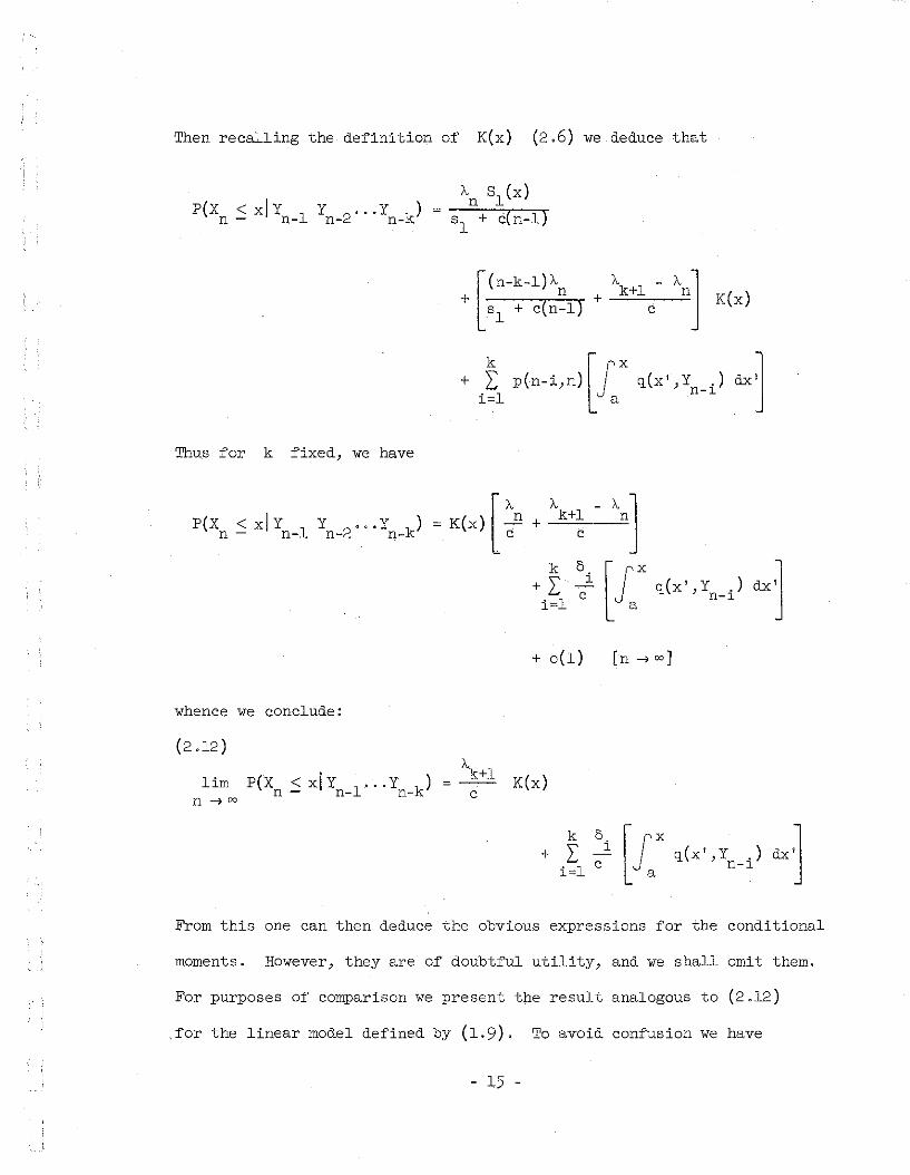
Then recalling the definition of K(x) (2.6) we deduce that
A.n Sl(x)
8 1 + c(n-l)
[.
(n-k-l)A. A._A.]+ s1 + c(n~1) + -=:kcc+l::'c-,--:::.n K(x )
+ I p(n-i,n)[fx
'l(x',Y _,) dx]i=l a n ~
Thus for k fixed, we have
k 6+ L .2-i=l c
p(x <xly 1 Y 2'''Y k) =K(x)[A.n
+n - n- n- n- . cA.k+~ - \]
[J:x
'l(x' ,Yn- i ) dxJ
whence we conclude:
(2.12)A.k+lc
+ 0(1)
K(x)
[n--'>oo]
From this one can then deduce the obvious expressions for the conditional
moments. However, they are of doubtful utility, and we shall omit them.
For purposes of comparison we present the result analogous to (2.12)
.for the linear model defined by (1.9). To avoid confusion we have
- 15 -

placed a superscript L on the response random variables corresponding
to the linear model. We have:
(2.13) lim F(X~ ~ xIYn~l"'Yn_k) = (l_S)k-l K(x)n-->oo
q(x' ,Y, .)n-l
The proof parallels the proof of (2.12).
We next wish to derive joint distributions for successive reinforce-
ments. In principle we can derive asymptotic joint distributions such
as
The general expression for arbitrary k is too complicated to be
meaningful. We will indicate the method by deriving the result for
k = 2, and we will note the analogous result for k = 3. For k = 2
we have:
{[n-l JX ' ][n-2 JX
= E i~l p(i,n) a 1 q(x,Yi ) dx i~l p(i,n-l) a 2 q(x,Yi )
+ 0(1) [n-->oo]
- 16 -

However, we recall that the
distributed, and we define:
Y 'si
are independent and identically
(2.15)
Thus:
:~: :~: p(i,n) p(j,n-l) E [JaXl 'l(x,Yi ) dx] E[~X2 'l(x,Yj ) dx]j;fi
+ 0(1)
n-l n-2L L p(i,n) p(j,n-l) K(xl ) K(x2 )i~l j~l
jfi
n-2+ L p(i,n) p(i,n-l) K(x
l,x2 ) + 0(1)
i~l
[n-l ~ [n-2 J~ K(xl ) K(x2 ) .L p(i,n) .L p(j,n-l)l~l J~l
From (2.5), recalling that A ~ A,n
n-lL p(i,n)i~l
we have
1~ - + 0(1)
c
" 17 -
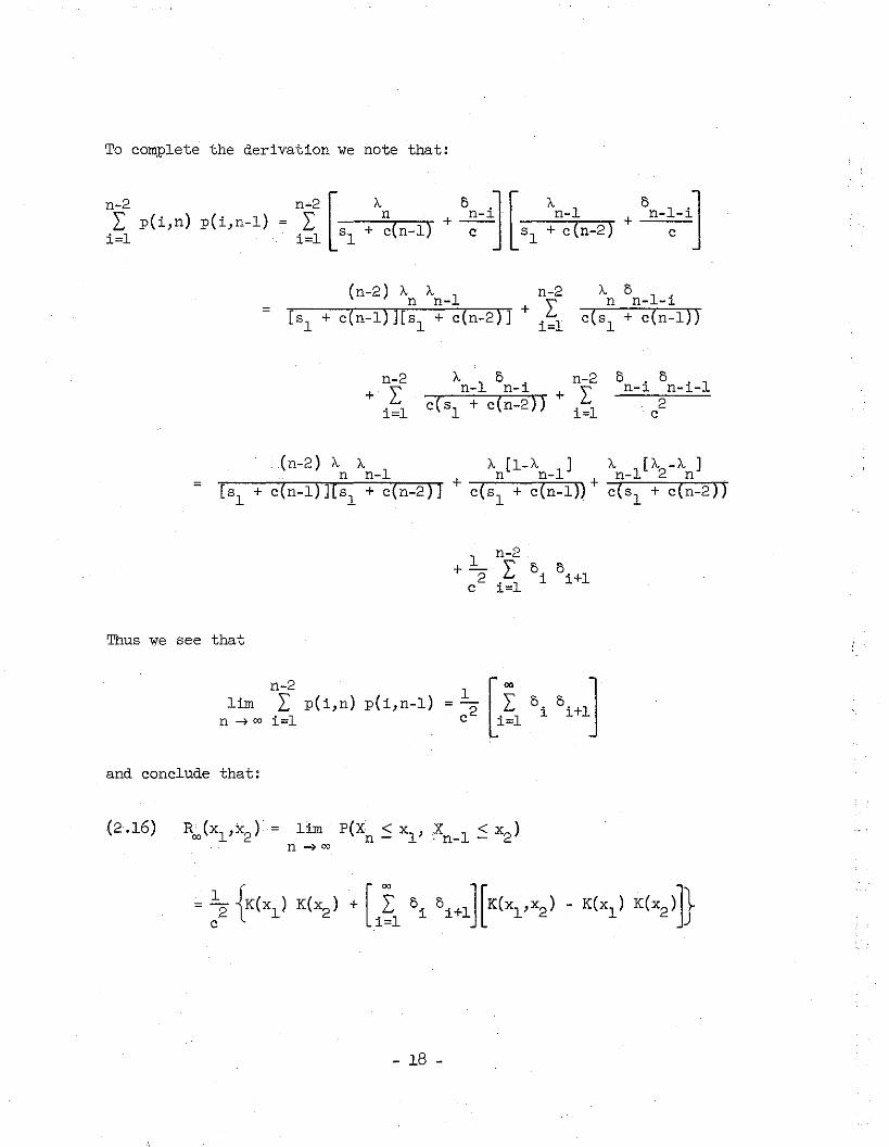
To complete the derivation we note that:
n-2L p{i,n) p{i,n-l)
i=l
).. 0n n-l-i
c{Sl + c{n-l))n-2L
i=l
(n-2)).. ).. 1n n-
c{n-l)J[sl + c{n-2)] +
o . 0 .n-1 n-1-1
2c
n-2L
i=l
).. 0n-l n-i
C{SI + c{n-2)) +
n-2+ L
i=l
=
(n-2)).. ).. ).. [1-).. 1] ).. [)..2-)..].,.-_,.-...,~,...",.:;no...-,",n.:.;-l"-r-."..,....,. + n n- + -Tn---=l=---,:::..-.,:.n"---;;"TT[sl + c{n-l) ](sl + c{n-2) J c{Sl + c{n-l)) c{Sl + c{n-2))
n-2+;L L
c2
i=l
Thus we see that
n-2 1lim L p{i,n) p{i,n-l) = c2
n --7 00 i=l
and conclude that:
(2.16) R)xl ,x2 ) = lim F{Xn :::: xl,Xn
_l :::: x2 )n .... ""
- 18 -
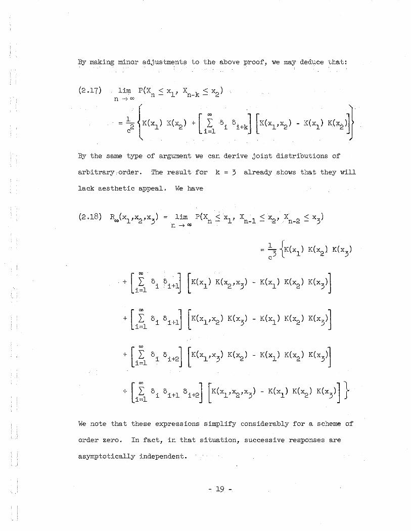
By making minor adjustments to the above proof, we may deduce that:
(2.17)
By the same type of argument we can derive joint distributions of
arbitrary order. The result for k = 3 already shows that they will
lack aesthetic appeal. We have
We note that these expressions simplify considerably for a scheme of
order zero. In fact, in that situation, successive responses are
asymptotically independent.
- 19 -
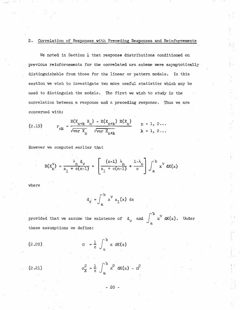
2. Correlation of Responses with Preceding Responses and Reinforcements
We noted ih Section 1 that response distributions conditioned on
previous reinforcements for the correlated urn scheme were asymptotically
distinguishable from those for the linear or pattern models. In this
section we wish to investigate two more useful statistics which may be
used to distinguish the models. The first we wish to study is the
correlation between a response and a preceding response. Thus we are
concerned with:
(2.19)/var Xn+k
n = 1, 2 .
k = 1, 2 ..
However we computed earlier that
Ie d= n V +
sl + c(n-l)l-Ie ] fb
+~ a xV dK(x)
where
Vx sl(x) dx
provided that we assume the existence of dv
and f b xV dK(x). Undera
these assumptions we define:
(2.20).
(2.21)
1 fb x dK(x)a = -c a
2 1 fb 2dK(x) - a2(r x
X ca
- 20 -

Clearly we may conclude that lim var Xn
and it remains ton ...ry. 00
consider E(X +k X ) - E(X +k) E(X ).n n n nAs is our custom we condition
on preceding reinforcements; and we have:
n-l+ I p(i,n)
i=l f bx q(x,Y.)
la
n+k-l fb ]}+ i~l p(i,n+k) a x q(x,\) dx
However, the reinforcements are independent, and we can therefore write:
:\:\ in n+k 1
[sl + c(n-l)][sl + c(n+k-l)]
n-lI p(i,n) c a
i=l
A dn+k 1
+ sl + c(n+k-l)
+ Sl + c(n-l)
n+k-lI p(i,n+k)
i=lc a
n-l n+k-l+ I I p(i,n) p(j,n+k)
i=l j=l(jfi)
2 2c a
n-l+ I p(i,n) p(i,n+k)
i=l
2 *c a
- 21 -

where we have defined and assumed the existence of:
(2.22 )
Recalling our computation of E(X )n
we then readily deduce that
From this, recalling the definition of p(i,n), we conclude that
+ c(sl + c(n+k-l))
Ie (Ie -Ie)n k+l n+k
+ c(sl + c(n-l))
n-l+ I
i;l
This equation seems a little too cumbersome to be of great value. How-
ever, we can deduce two asymptotic results which are of interest.
Recalling that lim Ie ; Ie we deduce that:n
n->'"
(2.24)
and
* 2 ['" J[0: -0:] I I). I). +ki;l 1 1
(2.25)
- 22 -
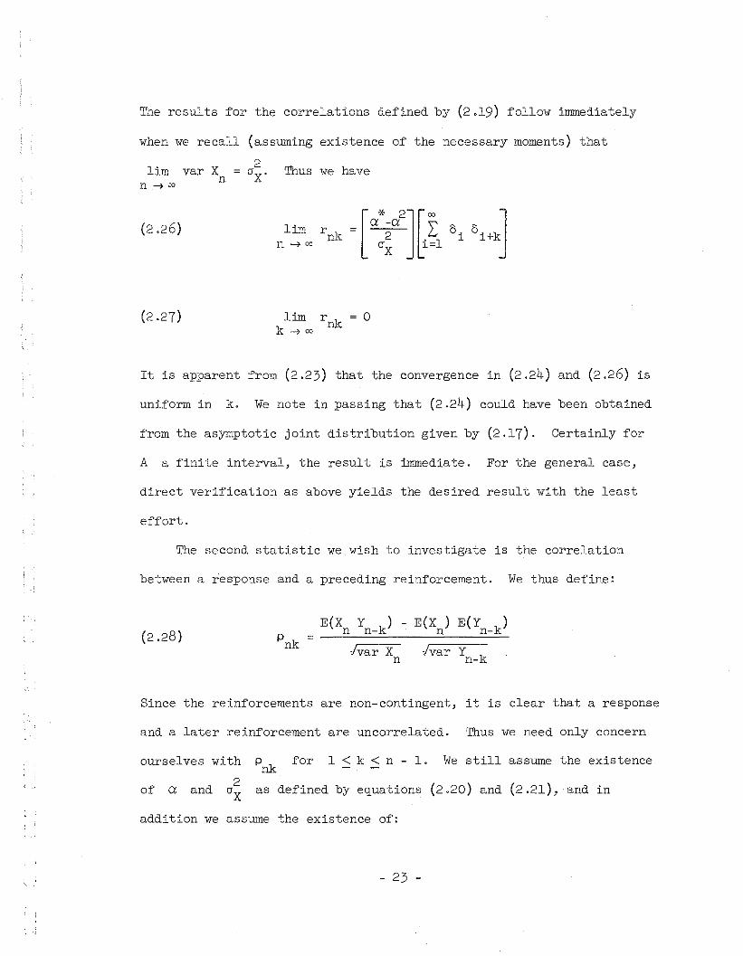
The results for the correlations defined by (2.19) follow immediately
Thus we havelim var Xn
when we recall (assuming existence of the necessary moments) that
2oX'
(2.26) limn~oo
(2.27) o
It is apparent frrnn (2.23) that the convergence in (2.24) and (2.26) is
uniform in k. We note in passing that (2.24) could have been obtained
from the asymptotic joint distribution given by (2.17). Certainly for
A a finite interval, the result is immediate. For the general case,
direct verification as above yields the desired result with the least
effort.
The second statistic we wish to investigate is the correlation
between a response and a preceding reinforcement. We thus define:
(2.28)E(Xn Yn- k) - E(X
n) E(Yn_k)
Ivar X Ivar Y kn n-
Since the reinforcements are non-contingent, it is clear that a response
and a later reinforcement are uncorrelated. Thus we need only concern
We still assume the existencel<k<n-l.forPnk
as defined by equations (2.20) and (2.21), and inof a and
ourselves with
addition we assume the existence of:
- 23 -
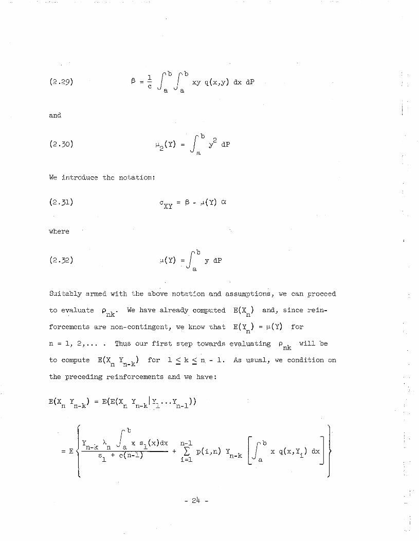
(2.29)
and
f3
(2.30 ) Jb
l dPa
We introduce the notation:
where
(2.32)
Suitably armed with the above notation and assumptions, we can proceed
forcements are non-contingent, we know that
to evaluate We have already computed E(X) and, since reinn
E(Y ) = ~(Y) forn
n = 1,2, .... Thus our first step towards evaluating Pnk will be
to compute E(Xn Yn
- k ) for 1 < k < n - 1. As usual, we condition on
the preceding reinforcements and we have:
= En-l
+ I p(i,n) Yn- ki=l
- 24 -

However, the reinforcements are independent and identically distributed
according to P. Thus:
A f.l(Y) dn 1 +
sl + c(n-l)
n-lI p(i,n) f.l(Y)
i=l( ifn-k)
[~b~b x 'L(x,y) dx dP]
+ p(n-k,n) [~b~b xy 'L(x,y) dx dP]
dx dP =Jb xdK(x)a
= a c
and we may thus write the above expression as:
An f.l(Y) dlsl + c(n-l) l
'- (n-l) A+ n
sl + c(n-l)
+ p(n-k,n) [c ~ - f.l(Y) a c]
(where we have used (2.5)). However, using (2.31) and the fact that:
E(X )n
we may conclude that:
Thus, using the definition of p(i,n) we have:
- 25 -
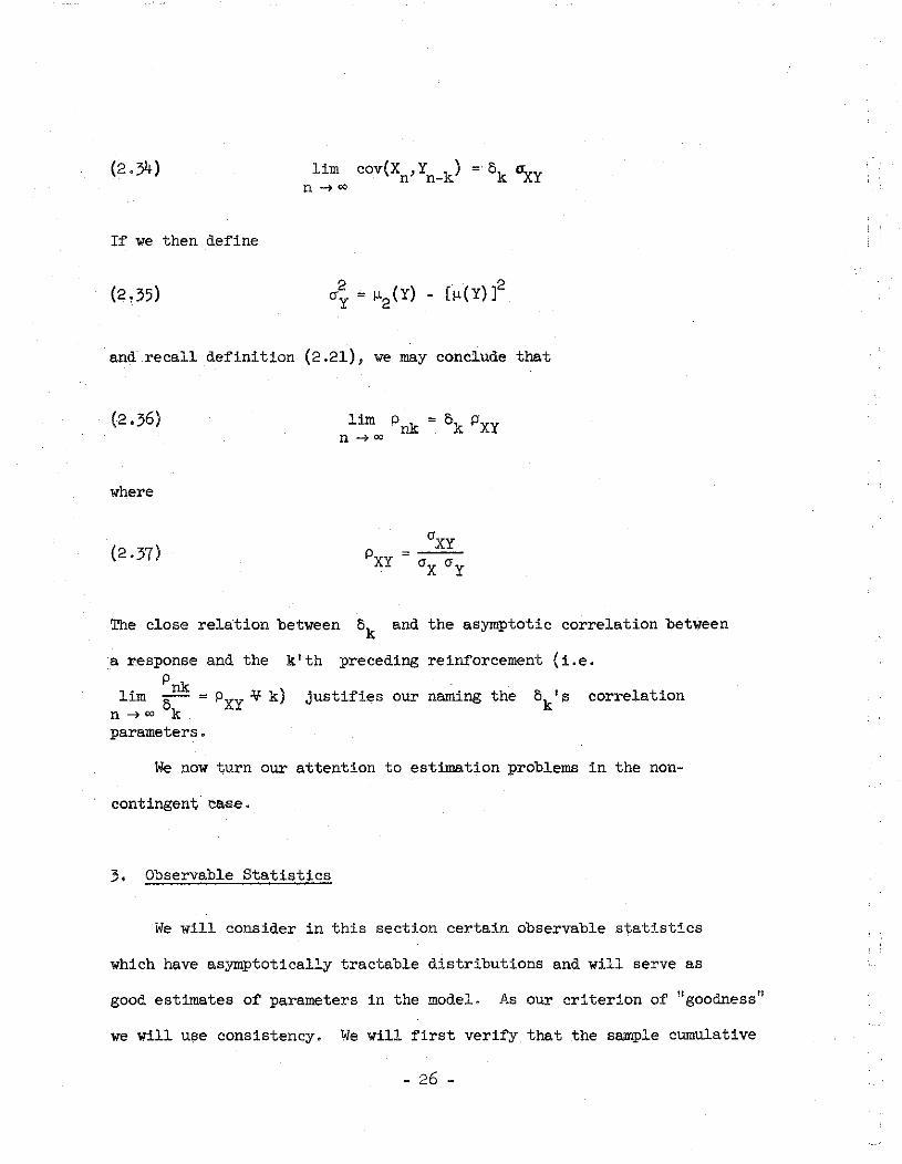
(2.34 )
If we then define
(2,35)
lim cov(Xn,Yn_k ) = Bk UXYn -> 00
and recall definition (2.21), we may conclude that
where
(2.37)
The close relation between Bk and the asymptotic correlation between
k'th preceding reinforcement (i.e.a response and thePnk
lim 8 = PXY ¥ k)n--7 OO kparameters.
justifies our naming the B 'sk
correlation
We now i;urn our attention to estimation problems in the non-
contingeni; ca~e.
3, Observable Statistics
We will consider in this section certain observable statistics
which have asymptotically tractable distributions and will serve as
good estimates of parameters in the modeL As our criterion of "goodness"
we will use consistency. We will first verify that the sample cumulative
- 26 -

distribution function of a protocol provides a good estimate of the
asymptotic response distribution (i.e. 1 K(x)). To prove this wec
first recall the definition
where
'R (x)n
1 nn I
i=lE(X. - x);
~xda,b]
E(X) = 0 X > 0
= 1 x < 0
Clearly E[E(X. - x)] = R.(x) and, by our usual procedure (i.e.,~ ~
conditioning on preceding reinforcements), we may compute the covariance
between E(X - x)n
and E(X k - x).n+ We have
E[E(X -x) E(X +k - x)] = E[E[E(X -x) E(x k-x)!Y, Y2 ···Y +k 1])n n n n+ ..L n-
[
Ien+k 81 (x)X . +
sl + c(n+k-l)
n+k-l (XI p(i,n+k)
1=1 \. a
Thus using methods exactly as those used to obtain (2.23) we obtain:
- 27 -
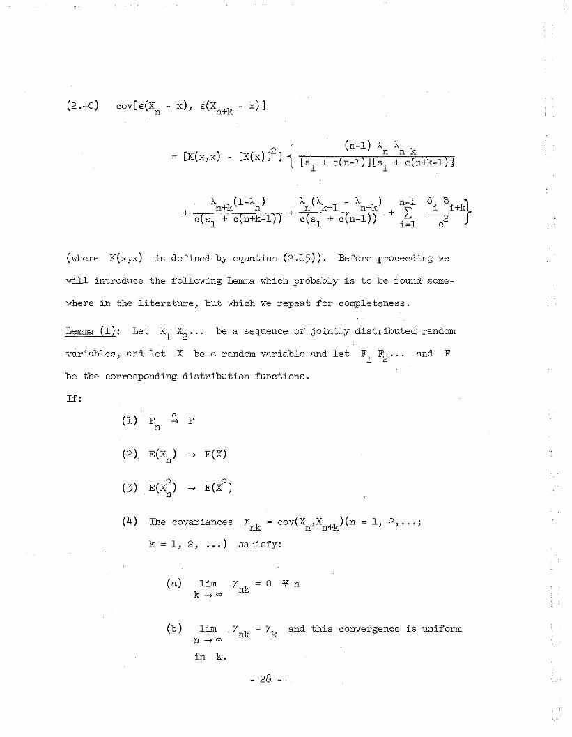
(2.40) cov[ €(Xn - x), €(Xn+k - x)]
{(n-l) A A k
[K (x, x) _ [K (x) ]2 ] .,.......--,--,---:..."..".,.--,"n'---,'n=..:+.=;--,-"..,....,[sl + c(n-l)][sl + c(n+k-l}]
5 5 1i 2 Hk
Jc
A (A - A )n k+l n+k
+ c(sl + c{n-l))
A (I-A)n+k n
+ c(Sl + c{n+k-l}}
(where K(x,x) is defined by equation (2.15». Before proceeding we
will introduce the following Lemma which probably is to be found some-
where in the literature, but which we repeat for completeness.
Lemma (1): Let Xl X2... be a sequence of jointly distributed random
variables, and let X be a random variable and let Fl
F2
•.. and F
be the corresponding distribution functions.
If:
(1) F .s Fn
(2 ) E(X) --> E(X)n
(3)
(4) The covariances Ynk
~ cov(Xn,Xn+k)(n ~ 1,2, ... ;
k ~ 1, 2, ... ) satisfy:
(a) lim Ynk
~ 0 ¥ nk-->oo
(b) lim. Ynk
~ Yk
and this convergence is uniformn-->oo
in k.
- 28 -
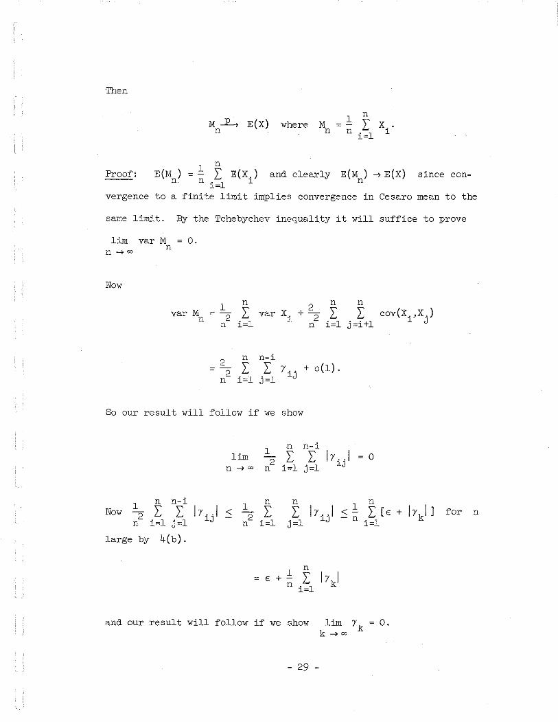
Then
M -.L, E(X)n
1 nwhere M = L Xi 0
n n i=l
Cesaro mean to the
since con-and clearly E(M) ~E(X)n
1 nE(M) =- L E(X.)
n. n i=l 1
vergence to a finite limit implies convergence in
Proof:
same limito By the Tchebychev inequality it will suffice to prove
lim var M = O.nn ~ 00
Now
var Mn
n
= \ Ln i=l
+~var Xi 2n
n
Li=l
n
Lj=i+l
cov(X. ,X.)1 J
n
Li=l
n-iL )' ij + 0(1) 0
j=l
So our result will follow if we show
lim 12
n
n n-iL L 1)' .. 1
i=l j=l lJ= 0
1 n n-iNow 2" L L I )' .. 1
n i=l j=l lJ
large by 4(b) 0
1< "2
n
n
Li=l
n
Lj=l
I I <!)' ij - n for n
1E +
n
n
Li=l
and our result will follow if we show lim)'k 00k~oo
- 29 -

Suppose Yk.4 0 then ¥E there exists an arbitrarily large k such
Choose n such that Iy - Y I < ~ ¥k [this isnk k 2
possible by 4(b)] then for this n by (A) we cannot have 4(a)
Contradiction. Yk
-> O. Q.E.D.
Now we wish to check whether the conditions of the Lemma are
satisfied by the sequence (E(Xi
- X)}~~l' (1), (2), and (3) are
trivially satisfied where the limiting random variable is a Bernoulli
random variable equal to one with probability 1- K(x)c
and zero otherwise.
The Ynk's were computed in equation (2.40), and we easily verify that
4(a) and 4(b) hold. 4(a) directly from (2.40) and 4(b) because
(n-l) A An n+k
[sl + c(n-l)][sl + c(n+k-l)]
A (l-A)n+k n A (A - A )n k+l n+kc(sl + c(n-l)) +
n-l2::j~l
00
2 2 2+ 2 2:: 5. 5< + +2 2 2 J j+k
c (n-l) c (n-l) c (n-l) j~n
600
< 2 + 2:: 5.c (n-l) j~n
J
and this is uniform in k. Thus we may apply the Lemma and conclude
(2.41) I': (x)..E...., ! K(x) ¥xEAn c
Our next interest is in the sample protocol moments. We define those we
will be chiefly interested in as follows
- 30 -
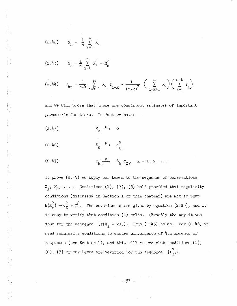
1 n(2,42 ) M ~ L X.n n
i~ll
1n
I if(2,43) S ~ Ln ni~l
l n
1n
1 (n ) (n-k )(2,44) C~ n-k L x, y - 2 L x. L Y..kn
i~k+ll i"k ( n-k) i~k+l l i~l l
and we will prove that these are consistent estimates of important
parametric functions. In fact we have:
(2.45)
(2.46)
(2.47)
M L 0:n
S L 2an X
C L 1) a XY k 1, 2, ...kn k
To prove (2.45) we apply our Lemma to the sequence of observations
Xl' X2 ' .... Conditions (1), (2), (3) hold provided that regularity
conditions (discussed in Section 1 of this chapter) are met so that
E(~) ~ a~ + 0:2
. The covariances are given by equation (2.23), and it
is easy to verify that condition (4) holds. (Exactly the way it was
done for the sequence [€(X. - x»)).l
Thus (2.45) holds. For (2.46) we
need regularity conditions to ensure convergence of 4th moments of
responses (see Section 1), and this will ensure that conditions (1),
(2), (3) of our Lemma are verified for the sequence
- 31 -
[I).l

Now
2 *c [V -2 { (n-l) \ ton+k
V] '[-sl---C+---Cc'(n--""""'l')']T[S";:l"--::+':':.";:c(T-n--:+7k-_l"-),,]
n-l+ L:
j=l
to (to - to )n k+l n+k
+ C(sl + c(n-l))
to k(l-to)n+ n+ C(Sl + c(n+k-l))
where
(2.48)
(2.49)
1 fbfb 2V = - x q(x}y) dx dPc a a
* 1Jab U:b
x2
q(x}y) dxrV =2" dPc
Again it is clear that condition (4) of the Lemma holds. Thus
1 n .2- L: r..J?., Vn i=l 1
and we already know that ML a.n
Applying Slutsky's
theorem we have Sl~??p ? 2
L. r. - ~ -"'-' V - ex- = aXn n i=l 1
which verifies
(2.46).
To verify (2.47) we first define
(2.48) P 1k}n = n-k
n
L: x. Y. ki=k+l 1 1-
(2.49) Sk}n
1 n= - L: X.
n_k i=k+l 1
(2.50 ) T 1k,n = n-k
n-kL: Yii=l
- 32 -
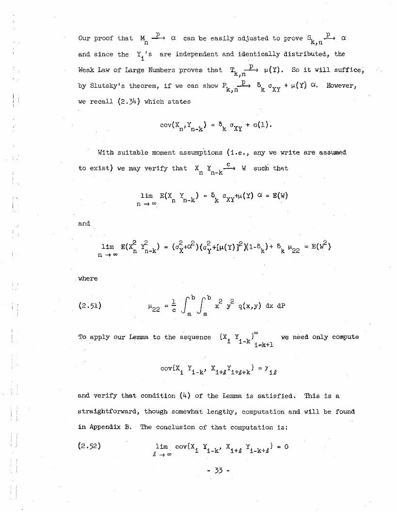
QUI' proof tha t M L Oi can be easily adjusted to prove S .R..., exn k,n
and since the Y 'si
are independent and identically distributed, the
Weak Law of Large Nwnbers proves that Tk ...12.... f.l(Y). So it will suffice,,n
by Slutsky's theorem, if we can show Pk,nL Ok CfXY + jJ.(Y) Oi. However,
we recall (2.34) which states
With suitable moment assumptions (i.e., any we write are asswned
to exist) we may verify that cX Y,--> W
n n-K.such that
and
where
"'222 2
x Y ~(x,y) dx dP
To apply our Lemma to the se~uence (Xi Yi_kloo
we need only computei;k+1
and verify that condition (4) of the Lemma is satisfied. This is a
straightforward, though somewhat lengthy, computation and will be found
in Appendix B. The conclusion of that computation is:
- 33 -

limi-7 00
where
(2,54 )
and where the convergence in (2.53) is uniform in £. Thus we may apply
the lemma and conclude
Whence, as suggested earlier, we may use Slutsky's theorem and obtain
the desired result (2.47),
4, Further Estimation
In Section 3 we developed estimates for several parametric functions
with at least two important exceptions, We did not discuss estimation
of "XY and1- 'l(x,y),c
Unfortunately, there is no simple estimate of
"Xy' One avenue of approach is open to us, nevertheless. We recall
and using this to compute an
that if ! 'l(x,y)c is known, then "XY
1will consist of estimating c 'l(x,y)
- 34 -
is computable, Thus our method
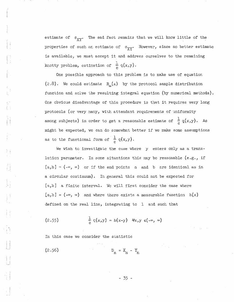
estimate of The sad fact remains that we will know little of the
properties of such an estimate ofaXY' However, since no better estimate
is available, we must accept it and address ourselves to the remaining
knotty problem, estimation of !. q(x,y).c
One possible approach to this problem is to make use of equation
(2.8). We could estimate R (x)00 by the protocol sample distribution
function and solve the resulting integral equation (by numerical methods).
One obvious disadvantage of this procedure is that it requires very long
protocols (or very many, with attendant requirements of uniformity
among sUbjects) in order to get a reasonable estimate of 1- q(x,y).c
As
as to the functional form of
might be expected, we can do somewhat better if we make some assmnptions
1 q(x,y) .c
We wish to investigate the case where y enters only as a trans-
lation parameter. In some situations this may be reasonable (e.g., if
[a,b] ~ (_00, 00) or if the end points a and b are identical as in
a circular continuum). In general this could not be expected for
[a,b] a finite interval. We will first consider the case where
[a,b] (_00, 00) and where there exists a measurable function h(x)
defined on the real line, integrating to 1 and such that
(2.55) 1 q(x,y) ~ h(x-y) ¥x,y e(-oo, 00)c
In this caSe we consider the statistic
D ~ Xn n
- 35 -
yn

Now we know that
E(D )n
A d n-ln 1 \'
; -s-l-+::"--c'(=-n--:1") + i:-l p ( i, n) [E {J:bx q(x,Y.)
1
but making use of (2.55) we have
q(x, Y.) dx1
+ C Jb x h(x) dxa
We introduce the notation
and we see that:
E(D )n
and clearly
lim E(D ) ; mn 1n -> 00
In general we have
- 36 -

We recall X and Yare independent and that (assuming existencen n
of the necessary moments):
__ JbJb xV h(x-y) dx dPa a
and thus we have
The moments of Yare known and thus VD may be used as an estimaten
of the linear combination of m.'s given by the right side of e~uation~
Needless to say, we would like consistent estimates of the m.Ts.~
To show that we can get them we must consider
and verify that the conditions of our Lemma are fulfilled. This com-
putational exercise is omitted. We then define
(2.60) Iin,V1 n
~ Xl 2:i~l
- 37 -

and conclude that
(2,61)
Thus, using Slutsky's theorem, we have consistent estimates for the
m,'s, although we still remain ignorant about the exact form of h(x),l
However, this approach would be of use if we assumed h(x) to be of known
form with moments depending on a few parameters,
For the case of a finite continuum with identical end points the
analysis which led to equation (2,61) is no longer valid, In this case
one is forced to assume a functional form for h(x) depending on a few
parameters, One then computes theoretical response moments as functions
of these parameters, substitutes the observed response moments and solves
for the parameters, This is the approach used in Appendix A" If the
end points are not identical, we cannot, as we 'earlier noted, expect
Y to enter in1c
q(x,y) only as a translation parameter, For this
case the solution of the approximate integral equation obtained from
(2,8) seems the only possible approach,
- 38 -

CHAPTER III
BEHAVIOR OF THE MODEL UNDER CONTINGENT REINFORCEMENT
We have seen that with non-contingent reinforcement, the analysis
of the correlated urn scheme is quite straightforward. The question
arises of what happens if the reinforcement distribution does depend
on preceding responses and/or reinforcements. This is the case of
contingent reinforcement. As might be expected, the analysis is more
complicated for this case. In fact, only for certain types of contingent
reinforcement will a limiting response distribution exist. We will
chiefly concern ourselves with the case of simple contingent reinforce-
ment. By this we mean: there exists a family of density functions
f(ylx) defined on [a,b] and indexed by xE[a,b] such that
p(y < ylXn - n
x) = JY f(y' Ix) dy'a
In Section 2, where we develop sufficient conditions for the existence
of a limiting response distribution, we will consider more complicated
contingent schedules; but our main concern is with the simple contingent
case.
1. Asymptotic Response Distribution
As has become our custom we let R (x) = p(X < x) and we aren n-
interested in the existence of a distribution function R (x) with the00
property that R (x)~ R (x)n 00
in the case of simple contingent
- 39 -

reinforcement (defined above). Now the reinforcements are no longer
independent and identically distributed. Nevertheless, we can still
condition on preceding reinforcements and responses, and we have:
R (x) = p(x < x)n n -
{
AS (x) n-l fX }=E. n+l(_l)+ L p(i,n) q(x',Y.)dx'
sl c n i=l a l
where
\ Sl(x)
sl + c(n-l)
n-l+ L p(i,n) E(Z.(x))
i=l l
Now
Z.(x) =fx q(x,Y.) dxl l
a
E(Z.(x)) = E[E(Z.(x)lx.)]l l l
i = 1, 2, ...
Substituting this value for E(Z.(x)) in our expression for R (x)l n
- 40 -
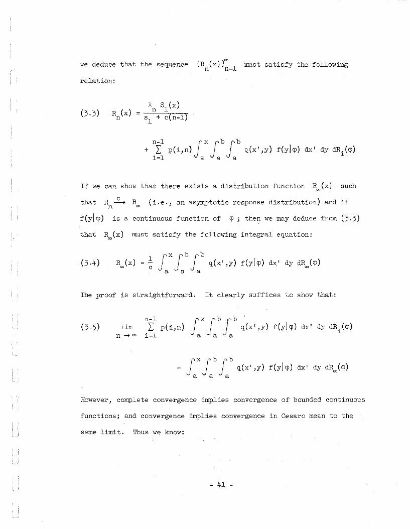
we deduce that the sequence (Rn(x)):=l must satisfy the following
relation:
R (x)n
\ 81 (x)
sl + c(n-l)
If we can show that there exists a distribution function R (x) such00
that R c R (i.e., an asymptotic response distribution) and if---->n 00
f(yjcp) is a continuous function of cp ; then we may deduce from (3-3)
that R (x) must satisfy the following integral equation:00
JXJbJbRoo(x) = ~ q(x',y) f(y[CP) dx' dy dRoo(cp)a a a
The proof is straightforward. It clearly suffices to show that:
limn-lI p(i,n)
i=l JXJbJb 'q(x' ,y) f(yjcp) dx' dy dRi(cp)
a a a
However, complete convergence implies convergence of bounded continuous
functions; and convergence implies convergence in Cesaro mean to the
same limit. Thus we know:
- 41 -
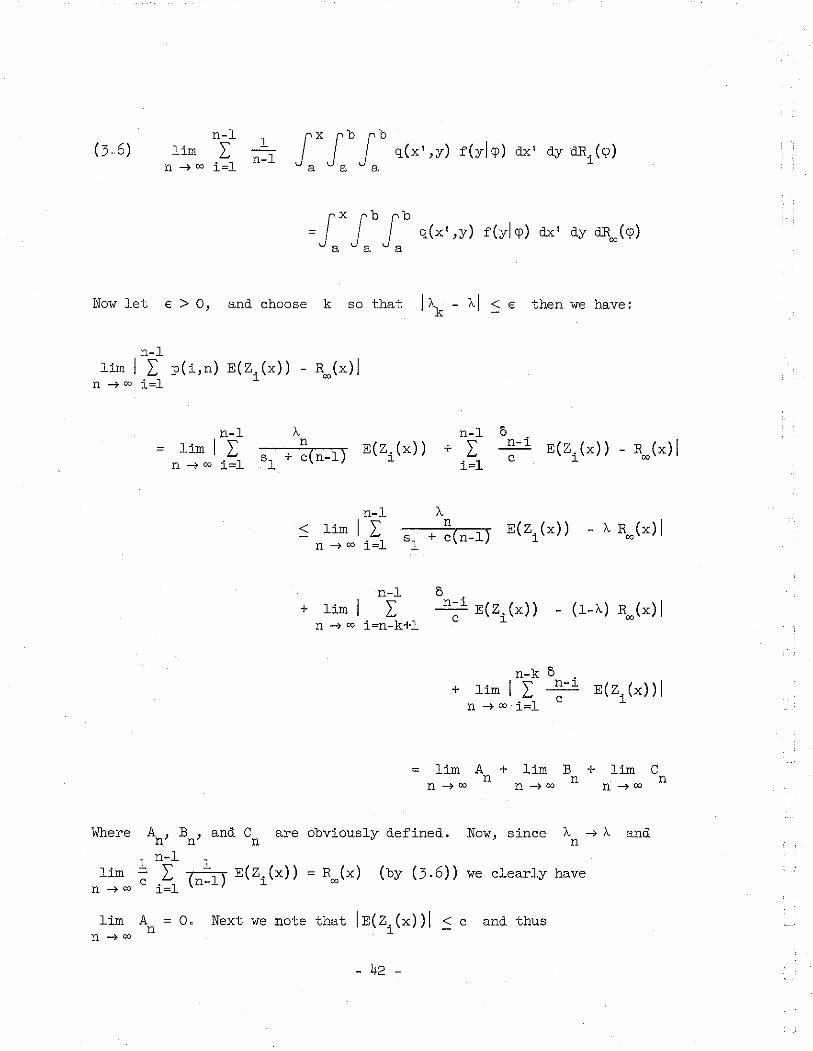
n-llim I
n ~ co i=l
1n-l
Now let € > 0, and choose k so that IAk
- AI < € then we have:
n-llim I I p(i,n) E(Z.(x))
n -700 i=l· 1.- R (x) I
00
n-l= lim I I
n -7 00 i=l
An E(Z. (x))
l
n-l+ I
i=l
6n-ic
E(Z.(x)) - R (x)1l 00
n-l< lim I I
n -7 00 i=l
An E(Z.(x))
l- A R (x) I
00
n-l+ lim I I
n -> 00 i=n-k+1
6 .~ E(Z.(x))
c l- (i-A) R (x) I
00
n-k 6 .+ lim I I n-l
n -700 i;;:;l C
E(z.(x))1l
= lim A + lim B + lim Cn n nn -7 00 n -7 00 n---t 00
Where A, B , and C are obviously defined.n n n1 n-l 1
lim - I r="l E(Z.(x)) = R (x) (by (3.6))c. ~n-.L) 1. con -700 1=1
Now, since
we clearly have
and
n -> 00
lim A = 0. Next we note that IE(z.(x))1 < c and thusn l
- 42 -

Finally
A < € for all (large enough) n.
Bn
k-llim I 2:
n ~ 00 i=l
k-l< 2:
i~l
6
2 [lim !E(Z .(x)) - c R (x)l] + €C n-1 00n-'>oo
where we have used the fact that lim! E(Z (x))c n
n-'>oo
verified (3.5) and (3.4) follows trivially.
R (x). Thus we have00
In the remainder of this chapter we will concern ourselves with the
problem of sufficient conditions for the existence of a limiting response
distribution. Before this, we wish to consider some implications of
equation (3.4) (Which we know the limiting response distribution, if it
exists, must satisfy). It was conjectured (Suppes, 1959) that the
asymptotic response distribution of the linear model with simple con-
tingent reinforcement would satisfy equation (3.4). Under some restric-
tive hypotheses, the result is proved by Norman (1964). The general
result for the linear model remains unproven. Given that equation (3.4)
holds, we are faced with a difficult problem when we try to estimate
! q(x,y). If we assume q(x,y) and f(yl~) are each continuous inc
both variables, it is easy to verify that the asymptotic response density
r(x) satisfies:
- 43 -

(3·7)
where
r(x) ~Jb g(x,cp) r(cp) dcpa
(3.8) g(x,cp) ~ Jb q(x,y) f(yjcp) dya
and b. (i1
Now (3.7) is a classical integral equation and is solvable for certain
functional forms of g and f. (For example if g(x,cp) is degenerate,
by which we mean there exist continuous functions a.(i ~ 1, 2, ... n)1
n1,2, ... n) such that g(x,cp) ~ L a.(x) b.(cp)). Our
i~l 1 1
procedure for testing would therefore be to assume a functional form
for 1c q(x,y) probably with y as a translation parameter and depend-
ing on a parameter related to the variance. Since f(ylcp) is known,
we then would know g(x,cp). Then solve (3.8). Hopefully our choice of
functional form for ~ q(x,y) and our reinforcement choice f(ylcp)
will allow an analytic solution. Then we could compare moments of this
derived asymptotic response density with the observed response moments.
The reader is referred to Suppes and Frankmann (1961) for a discussion
1of the effects of the exact form of - q(x,y) on the shape of the
c
asymptotic distribution. Their comments refer to the linear model, but
analogous results hold for the correlated urn scheme. They conclude
that the important factor in1c q(x,y), provided y is a translation
parameter, is its variance. With this in mind, for
with identical end points, one is prompted to assume
form
- 44 -
[a,b] ~ [0, 211 ]
1c q(x,y) has the

1c
CJ.(x,y)1
= k(n)
2n
integer valued parameter to
where,
k(n) lfbis chosen such that c CJ.(x,y) dxa
be estimated from the
= 1 and n is an
data. For a large
family of trigonometric reinforcement functions, f(yl~), this will
yield degenerate kernels. It now remains to discuss conditions which
will guarantee the existence of a limiting response distribution.
2. SUfficient Conditions for the Existence of an Asymptotic Response
Distribution
Our aim in this section is to develop a set of sufficient conditions
(relating to the reinforcement schedule) which will ensure the existence
of an asymptotic response distribution for the correlated urn scheme with
contingent reinforcement. The tool we make use of is a theorem due to
Ionescu Tulcea (1959) in a modified form due to Norman (1964). The
theorem is applicable to any chains of infinite order. We will use
Norman's notation as much as possible.
be a discrete parameter stochastic processLet Zl' z2' Zy'"
with state space Z. Let e be the Borel field of subsets E of Z
for which transition probabilities p(Z 1 EElz Z l"'Zl)n+ n n-are
defined, We use the notation:
= p(z 1 EElz z l"'Zl)n+n n-
- 45 -

(3.11) = p((Z k"'z 1) € Biz Z l",zl)' B € ~n+ n+ n n-
Let Z be the collection of all possible finite histories of the process,00
for each positive integer
For any bounded functionz = U Zn,n=l
is measurable with respect to
we define a new function Uf by:
f on z whose restriction
n,
(3,12)
where
(Uf) ("2 )n
Z + z = (z z ... z)n+l n n+l n 1
E - f( Z 1 + Z )- n+ nzn
if z = (z Z 1'" Zl)n n n-
and where the expectation is computed with respect to the probability
measure PE(Zn), Clearly, it follows that
k (U f)(z )
n=E(k)f((Z Z z) +-z)
k 1 ", 1- n+k n+ - n+ nzn
where the expectation is taken with respect to the probability measure
PK,B(zn) defined by (3.11). We then have:
Theorem 1: - If
00
(a) < 00 where
sup
(b) there exists a probability measure ~ on e and a
positive number S such that
- 46 -

( c) lim (j). 0 wherej~oo J
sup/ feZ + z') f(z + Zll)!(j)
zj -j z' -II€ z; Z, Z E
Uoofthen there exists a constant such that
uniformly in z as n ~OOQ
'"Uf
We note here that both Ioneseu-Tulcea's original theorem and
Norman's modification give estimates of the rate of convergence. For
application to the correlated urn scheme, it will not be possible to
give a meaningful rate of convergence. By this we mean that the rate
of convergence depends, in a rather complicated way, on the sequence of
correlation parameters. Given a particular set of values for these
parameters, then a quick reference to either of Ioneseu-Tulcea's and
Norman's papers will enable one to obtain an estimate of the rate of
convergence, For this reason, we will omit further comment on rates
of convergence.
We can apply Theorem 1 to obtain a set of sufficient conditions
for the existence of a limiting response distribution for the correlated
urn scheme with contingent reinforcement. We denote the conditional
density of Yn
given x Y 1 X 1" 'Yl Xln n- n-by f('/X Y lX 1'"n n n- n-
Theorem 2: - For the correlated urn scheme with a contingent reinforce-
forcement schedule,sufficient conditions for the existence of a distri-
but ion function R",(x) independent of Rl(x) with the property that
- 47 -
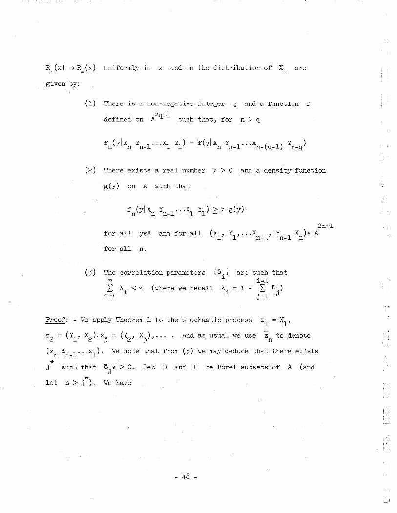
R (x) ~R (x) uniformly in x and in the distribution of Xl aren 00
given by:
(1) There is a non-negative integer q and a function f
defined on such that, for n > q
f (ylX Y 1" ,Xl Yl )n n n- f(y[ X Y l"'X ( 1) Y )n n- n- q- n-q
(2) There exists a real number Y > 0 and a density function
g(y) on A such that
for all yeA and for all2n+l
X )€ An
for all n.
(3) The correlation parameters (0. ) are such thatl i=l00
L A. <00 (where we recall A. = 1 - L 0.)i=l l l j=l J
Proof: - We apply Theorem 1 to the stochastic process zl = Xl'
(andAbe Borel subsets ofand EDLet0.* > O.J
such that
Z2 = (Yl ' x2 ), Z3 = (Y2 , X3
), .. · . And as usual we use zn to denote
(z Z l"'Zl)' We note that from (3) we may deduce that there existsn n-
*j
*let n> j). We have
- 48 -

=1D
n+ L p(i,n+1)
i=lf (yj"Z ) dy
n n
y f (1 'l.(X,y) dx) g(y) dyD E
Thus condition (b) of Theorem 1 is satisfied with
f.l(D X E) = ~ 1 (f 'l.(X,y) dx) g(y) dy.D E
Now if n', n" 2: £ > 'l. and z'n'
and Zlln" are such that
z', . = z"" ., 0::S j < £ then f, (il"Z',) = f ,,(y!"Z",,) and we have:n -J n -J n n n n
n' ~+ L p(n'+1-i,n'+l) 'l.(x,Y' '+1 .) f ,(y!"Z' ,)i=l n -~ n n
dx dy
n"L p(n"+l-i,n"+l)
i=l
- 49 -

where y'n '
y"nil ; y
nilc p(n'+l-i,n'+l) + L:
i;,gc p(n"+l-i,n"+l)
(CA )n'+l
""
nil+ L:
i;,g(
CA II )n +1 +81
+ cnfl
Now we recall that
for large £, the
A < "" and that this implies A -> o. Thusn n
two terms are negligible, and each of the next
two terms is bounded by A,g. Thus we may certainly conclude that
Thus condition (a) of Theorem 1 holds with
Now if we let fez); PDXE
(2) we verify (exactly as above) that con
dition (c) of Theorem 1 is satisfied with illj
; 6Aj
. We thus may apply
""the theorem and conclude that for any Xl € A there exists U PDXE
such that UnPDXE (Xl) -> U""PDXE
. Now we let D; A and E; [a,x]
""and denote U PAX[ a,x] by R)x).
- 50 -
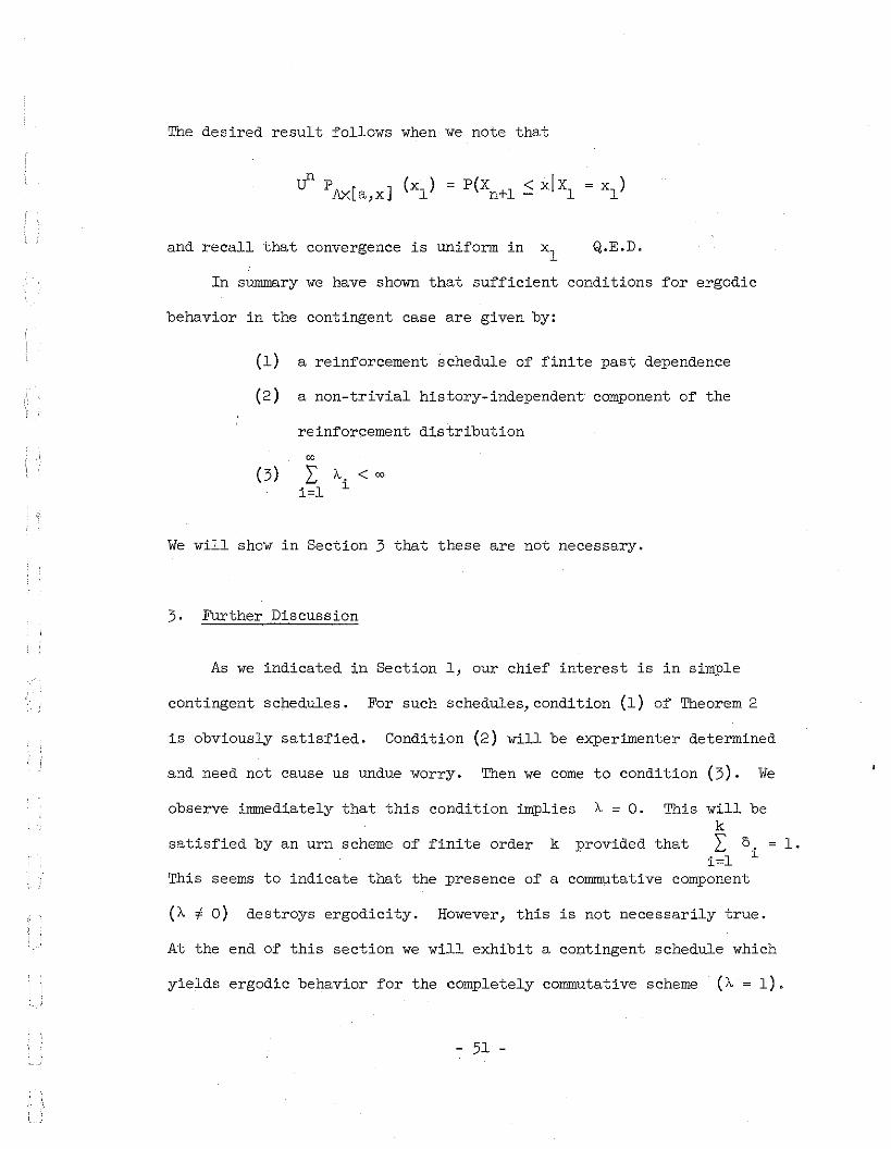
The desired result follows when we note that
and recall that convergence is uniform in xl Q.E.D.
In summary we have shown that sufficient conditions for ergodic
behavior in the contingent case are given by:
(1) a reinforcement schedule of finite past dependence
(2) a non-trivial history-independent component of the
reinforcement distribution
00
We will show in Section 3 that these are not necessary.
3. Further Discussion
As we indicated in Section 1, our chief interest is in simple
contingent schedules. For such schedules,condition (1) of Theorem 2
is obviously satisfied. Condition (2) will be experimenter determined
and need not cause us undue worry. Then we come to condition (3). We
observe immediately that this condition implies A = O. This will bek
satisfied by an urn scheme of finite order k provided that I o. 1.i=l 1
This seems to indicate that the presence of a commutative component
(A 1 0) destroys ergodicity. However, this is not necessarily true.
At the end of this section we will exhibit a contingent schedule which
yields ergodic behavior for the completely commutative scheme (A = 1).
- 51 -

Nevertheless, we can use Theorem 2 to verify that ergodicity obtains
under simple contingent reinforcement provided that the responses
depend only on a finite number (possibly or probably a large finite
number) of preceding reinforcements. Since memories in the real world
are finite, this restriction on the degree of past dependence is not
totally unappealing. We note for the case of a correlated urn scheme
of finite order k with A o and simple contingent reinforcement,
that the stochastic process zl
is a Markov process of order k. This suggests a method of testing
whether this type of model is applicable. We could partition A into
and define a Markov chaina finite number of subsets
where (l)n
Al
A2
•. .Ap
(j,k) if Y € A.n-l J
If the
0, ¥ i) and we will assume the
original process was of order k then the derived chain will be of the
same order. One could then apply standard X2
tests for the order of
the derived chain.
We conclude this chapter with the promised counterexample to the
necessity of the hypotheses of Theorem 2. We will consider a correlated
urn scheme of order 0 (i.e., 5i
reinforcements are simple contingent such that:
where a < p < band fl
, f 2 are densities defined on A = [a,b].
For this case we may rewrite (3.3) as follows:
~ 52 -

R (x)n
Sl (x) n-l= -s-+'=-c'(-n-""""l") + L:
1 i=l
If' we define
and
(3.16)
we may write:
(3.17) R (x)n
Setting x = P and applying (3.17) to both Rn(P) and Rn_l(P) we
deduce that:
We recall that gl(P) - c < O. It is then easy to verify (using (3.18))
that:
- 53 -

Rn
_l
(p) <g2(P)
implies Rn_l(P) < Rn(P) <g2(P)
c - gl (p) c - gl(P)
Rn_l(P)g2 (p)
implies Rn
_l
(p) > Rn
(p) >g2 (p)
>-~ c - gl(P)c - gl P
Rn_l(P)g2(P)
implies R (p)g2 (p)
c - gl(P) n c-gl(p)
Thus lim R (p)n
n~co
then deduce that:
Going back to equation (3,17) we may
. gl(X) [. g2(P) ]lim R (x) = -- ( )n c c-glPn-->oo
g2(X)+-
c
and the limiting distribution does not depend on Rl(X), Clearly this
example violates condition (3) of Theorem 2.
- 54 "

CHAPTER IV
TESTS, GENERALIZATIONS, A1ID APPLICATIONS
Several times in the earlier chapters we have suggested possible
tests to determine whether a particular consequence of the correlated
urn scheme is upheld by a given set of data. In the first section of
this chapter we will outline a method of constructing an (almost)
arbitrarily stringent test based on sequential dependencies. Unfortu
nately, measures of the stringency of tests of learning models are
essentially non-existent; so that belief in the preceding statement is
a matter of personal preference. If one has great faith in minimum
- X2 estimates, then one would believe in the stringency of the
suggested test. An alternative procedure is suggested which avoids
minimum - X2
antics, but which is open to criticism from other direc
tions as we shall see. Sections 2 and 3 will be devoted to generalized
correlated urn schemes. Section 4 will consist of a brief discussion
of the application of the correlated urn scheme to two-person inter-
actions.
1. Testing the Model
The problem of testing continuous-parameter learning models is not
a particularly pretty one. The conditional predictions used in finite
cases are no longer meaningful, but the rationale behind them may be
used by utilizing the device of discretizing the range. To this end,
we partition [a,b] into I response subsets ~,A2, ••• ,AI' and we
- 55 -

also construct a second partition into J reinforcement subsets
Bl
, B2,oo.,BJ
(the two partitions can be identical if we wish). We
will restrict our discussion to the case of non-contingent reinforce-
ment. We are interested in statistics of the form:
p(X "A Iy 1" B ° ,0 ° 0' Y k" B, )n r n- J l n- Jk
where 1 < r < I and 1 < j < J, Y = 1, 2, ... ko- Y-
Since we are in the
non-contingent case, we know that the Yi's are independent and
identically distributed according to the probability measure Po We
introduce the notation
b, = P(B,)J J
Now
j = 1, 2, 0 • • J
p(X "A, Y 1" B1 '0. °Y k·€ BJ'k)n r. n- '1 n-P(Y 1" B, ,>0., Y k E B, )
n- J n- Jk1
= ( rrk ·b ,) -1 P(X € A , Y. 1 € B, , ... , Y kJ n r n- J1 n-p=l
However we have:
- 56 -

p(X E A , Y 1 E B. , ... , Y k € B. )n r n- J1 n- J k
= E(P(X E A, Yn
-1
€ B. , ... ,Y k€ B. IY1
y2 ... Yn
-1
))n r J1 n- J k -
= E [f f ... r [ len 8 1 (x)A B. J B. 8 1 + c(n-1)
r h J k
n-1+ L p(i,n)
i=l'l.(X,Y.)] dx dP l' .. dP k]J. n- n-
n-k-1+ L p(i,n)
i=l
k+ L p(n-i, n)
i=l
We then define:
(4.4)
(4.5)
i; 1 [ JAr J:b'l.(x,y) dx dP]=-- r=1,2 ... 1
r cO"XY
)' rj1 [I f 'l.(x,y) dx dP} 2 ... I= r = 1,
cO"XY b j A B.r J
j = 1, 2 ••• J
- 57 -
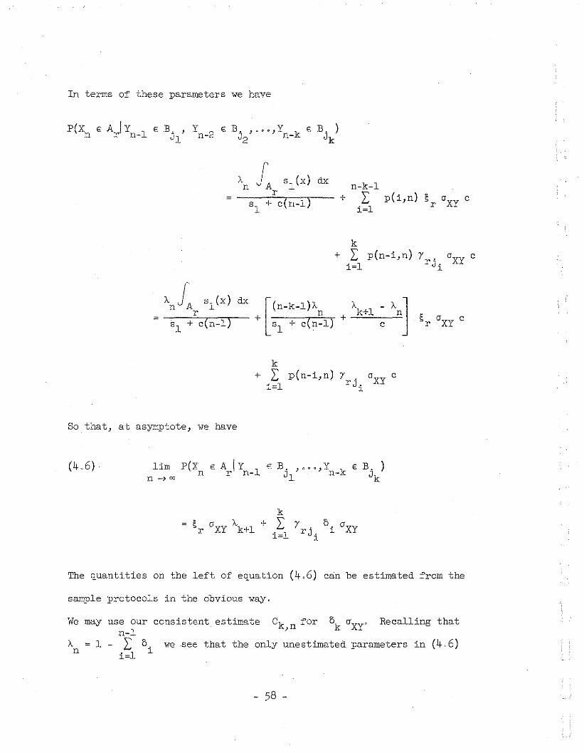
In terms of these parameters we have
p(x E A. IY . E:.B. , Y 2 € B. ," 0 , Y k e B. )n .r n-J. J1 n- J2 n- Jk
k+ L p(n-i,n)
i=l
\~ Sl(X) ax[(n-k-1))C )C \]r + n + k+l
Sr C1XY c= sl + c(n-1) sl + c(n-l) c
So that, at asymptote, we have
k+ L
i=lp(n-i,n) y . C1
XYc
rJ.l
11mn -~ 00
k+ L
i=l
The ~uantities on the left of e~uation (406) can be estimated from the
sample protocols in the obvious way 0
we see that the only unestimated parameters in (406)
We may use our consistent estimaten-l
)C=1-"6n L.- ii=l
Recalling that
- 58 -

are
I +
(s )1 and (lr o )1,J .r 1 J 1 1,
1J parameters. We can
Thus we have 1JK estimates depending on
then use minimum _X2 estimates of the
For this test, we select a functional form forof Chapter 2.
(Sr) and (l rj) to test the modeL
An alternative test is suggested by our discussion in Section 41c q(x,y)
with y entering as a translation parameter and depending on some
parameter w related to its variance. We then compute the asymptotic
response variance as a function of w; equate this to the observed
*response variance and solve for w. We denote the solution by w .
*With this value of w
if w is known, then
we may compute
1c q(x,y) is completely
and [l }1,Jrj 1 1,
determined) 0
(recall
Substituting
these computed values into the right hand side of (4.6) and substituting
Ck,n for ok 0XY' we obtain what we call the theoretical values for the
conditional probabilities. These may then be compared with the observed
values to test the model. This is the method used in Appendix A. We
intimated earlier that this method has drawbacks. The problem is that
there is no basis upon which to compare the theoretical and the observed
values. The degree of accuracy is not measurable. Nevertheless, this
method is useful for comparisons between models and, if "reasonable"
accuracy is obtained for repeated experiments, may be regarded as a
valid test.
- 59 -
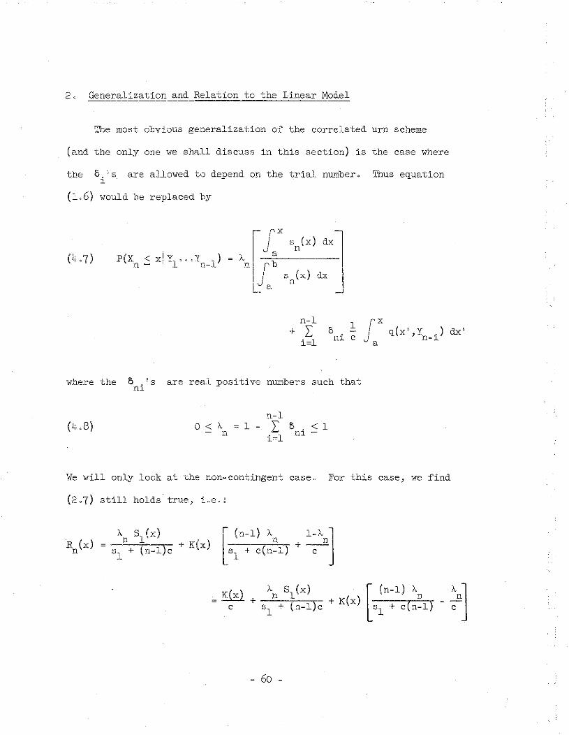
20 Generalization and Relation to the Linear Model
The most obvious generalization of the correlated urn scheme
(and the only one we shall discuss in this section) is the case where
the o 'si
are allowed to depend on the trial number, Thus equation
(106) would be replaced by
p(x < !v .- )'n - x, '"1 0
- • (n-l
n-l+ I
i=lD . 1
nl. C j Xq(X"y.)dx'n-~
a.
where the o 'sni
are real positive numbers such that
(4.8) O<A-ln
n-lI Dni < 1
i=l
We will only look at the non-contingent case. For this case, we find
(2.7) still holds true, Le.:
\\(x)sl + In-l}c
+ K(x)[
'_n-_1---,-)A--.::;n", + l-cAn]s1 + c(n-l)
\ 81 (x)
81
+ (n-l) c+ K(x)
- 60 -
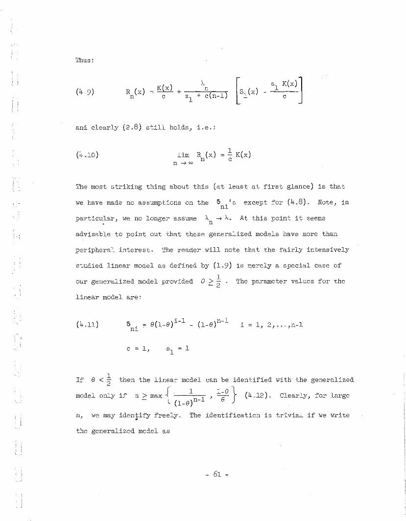
Thus:
A.R (x) ~ K(x) + --c-'n7-~
n c sl + c(n-ll
and clearly (2.8) still holds, i.e.:
(4.10) lim1
R (x) ~ - K(x)n· c
The most striking thing about this (at least at first glance) is that
we have made no assumptions on the 5 'sni
except for (4.8). Note, in
particular, we no longer assume At this point it seems
advisable to point out that these generalized models have more than
peripheral interest, The reader will note that the fairly intensively
scudied linear model as defined by (1.9) is merely a special case of
our generalized model provided e ~ ~ The parameter values for the
linear model are:
(4.11) i 1, 2, ... ,n-l
c 1, 1
If e < ~ then the linear model can be identified with the generalized
model only if n ~ max { 1 -1 ' le-e} (4.12). Clearly, for large(l_e)n
n, we may identify freely. 'The identification is trivial if we write
the generalized model as
- 61 -

)"n 81
(x)
sl + c(n-l)
n(x'Y.)dx'':1. } n-~
),.n
n
with the stipulation that
and
'rhis0<),. < 10n -
This is the same as (1.9) provided. ),.
( )1-1 no . = a l-a - - ,
nl n
yields condition (4.12). Clearly for the linear model ),. -> 0 andn
o . > 0 ¥ n,i. We also note that the asymptotic behavior of the linearnl
model will be indistinguishable from the asymptotic behavior of the
correlated urn scheme with parameters
Clearly the convergence of response moments for the model described by
(4.7) and (4.8) can "be verified as in Chapter 2 (With the same regularity
conditions). Needless to say we cannot repeat the remaining analysis of
Chapter 2 without further assumptions on the " ,u . SonJ.
In fact, just about
the only tractable case is when o . = 0 + 0(1)TIl i
and this case will, of
course, be asymptotically indistinguishable from the correlated urn
scheme as originally defined.
- 62 -

3. Fseudoreinforcements
The concept of pseudoreinforcement was introduced by Suppes and
Rouanet (1964)0 The concept was introduced in connection with the
linear modeL However, the rationale behind it applies equally well to
the correlated urn scheme. suggest that, although reinforcements
Yl , 72"'0 are given, the subject may react as if reinforcements
were given where the
preceding reiD~orcementso
Thus we have:
The
Zn
Z.'s are weighted averages ofl
Z 1 8 are called pseudoreinforcementsoi
kwhere I Po = 1.
i=O l
the distribution of
Clearly, since the distribution of
Z as a functl'on of P P Pn 0' 1'00" k
yn
is known)
is then knoWllo
For example, we easily deduce that, if the reinforcements are non-
contingent, then the pseudoreinforcements will be identically distri-
buted though no longer independenL Theoretically we could assume that
the subjects' responses are determined by equation (1.6) with r7 )i
replaced by [Zi J defined by (4014) 0 We could then compute conditional
probabilities of the type discussed in Section 1 of this chapter as
functions of PO' Pl
, o •• Pk
. Unfortunately, in actual practice this will
entail computation of (k + 1) - .:fold weighted convolutions of the
distribution of Y. Except for very special choices of the distribution
of Y (normal distributions are about the only ones that leap to mind),
this can be a Herculean task.
- 63 -
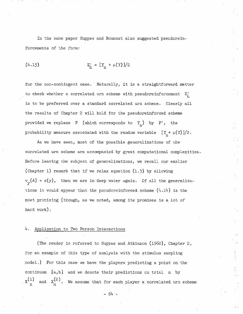
In the same paper Suppes and Rouanet also suggested pseudorein-
forcements of the form:
(4.15)
for the non-contingent case. Naturally, it is a straightforward matter
to check whether a correlated urn scheme with pseudoreinforcement z·n
is to be preferred over a standard correlated urn scheme. Clearly all
the results of Chapter 2 will hold for the pseudoreinforced scheme
provided we replace P (which corresponds to Y )n
by P' , the
probability measure associated with the random variable [Y + fl(Y) ]/2.n
As we have seen, most of the possible generalizations of the
correlated urn scheme are accompanied by great computational complexities.
Before leaving the subject of generalizations, we recall our earlier
(Chapter 1) remark that if we relax equation (1.3) by allowing
V (A) = c(y), then we are in deep water again. Of all the generaliza-y
tions it would appear that the pseudoreinforced scheme (4.14) is the
most promising (though, as we noted, among its promises is a lot of
hard work) .
4. Application to Two Person Interactions
(The reader is referred to Suppes and Atkinson (1960), Chapter 2,
for an example of this type of analysis with the stimulus sampling
model.) For this case we have the players predicting a point on the
continuum
and
and we denote their predictions on trial n by
We assume that for each player a correlated urn scheme
- 64 -

is applicable and that reinforcement is given to both players contingent
on both responsesQ Tnat is we assume~
(4016)
ax]
[i=1,2]
Where y(i) is the reinforcement given to player i on trial n. Wen
assume there exist two densities h(i)(y) [i = 1, 2J on [a,b] andofour families of densities h~i)(ylx) on [a,b] [i = 1, 2; j = 1, 2]
J
parameterized 'by x E[a,b] such that
(4017)
where
- 65 -

It will be seen that the interaction is obtained by reinforcing contin-
gent on both players' responses. We also note that we assume that the
responses on trial n are conditionally independent (given
[i = 1, 2] we may verify that, analogous to the result for
y(l) y(2)1 ' 1 '00
L: ),.(i) < 00
n=l n
(2) (1)Y2 ' •.• 'Yn-l' Y~~{ .). Provided that
the linear model, at asymptote R(i)(x) [i = 1, 2] satisfy:00
(4.18)
and
[i=1,2]
Naturally these will be difficult to solve unless we make very advanta-
1 (i)geous assumptions about the form of the functions ~ q (x,y)
cThe reader is referred to Suppes and Atkinson (1960) for
examples of particularly advantageous choices.
- 66 -
We have presented this application as an illustration of the re~~rk
that: in whatever situations a linear model (or a stimulus sampling
model) might apply, a correlated urn scheme deserves consideration. The
asymptotic response distributions are identical, but the urn scheme
exhibits more flexibility in dealing with se~uential statistics. The
similarity in range of applicability between the linear model and the
urn scheme is clearly attributable to the fact that the former is
asymptotically indistinguishable from a special case of the latter.
- 67 -

APPENDIX A
AN EMPIRICAL COMPARISON WITH THE LINEAR MODEL
In this section we will make use of the data collected by Suppes,
Rouanet, Levine, and Frankmann (1964), Our aim will be to compare the
second order conditional predictions assuming a correlated urn scheme
with the predictions obtained by the above authors assuming a linear
model, The reader is referred to their paper for a detailed description
of the experiment and for the analysis leading to the linear model
predictions. We will present here only those details necessary for
comparison 0
For'the experiment in question, the interval (a,b) was the circum-
ference of a circle and responses and reinforcements were measured in
radians (i,e., a = 0, b = 2n), Non-contingent reinforcement was used
with reinforcement density:
I
(Al) f(y)
(It - y);
(y - n)
(2lt - y);
- 68 -

We assume
~ 'l(x,y) l2a !x - yl < a
0; Ix - yl > a
where Ix - yl is computed modulo 2n and where a is a parameter to
be estimated from the data, Using (2.8) we readily verify that the
asymptotic response density function is given by:
(A3) r(x) 1 2 2= 2 (x + a );
an0< x < a
2x= n2
;
1 1 [( n 2+ a
2];
n n2 2 - x )
2- a < x < .-
n 2all
r(n - x)n
; -<x <n2 -
provided tha't
r(x - n)
r(2n - x) ;
na<4
n<x<3n2
As we shall see our estimate of a is less than ~ so that (A3)
is valid.
- 69 _

We define the auxiliary random variables *X ,n
as follows:
*X in
*y in
if
if
(i-l}re < X < .ire2 n - 2
(i-l}re < y < in2 n - 2
i 1, 2, 3, 4
i lJ 2, 3J 4
and we will consider the statistics:
* il y* 1 * i = 1, 2, 3, 4l(A4) lim p(x = = j, y = k)n n- n-2 j 1, 2, 3, 4'n -> 00
k = 1, 2, 3, 4
Referring to equation (406) we see that
(A5) *lim P(Xnn--7 00
where
(A6) fb ~ q(x,y} f(y} dy dx;a
i = 1, 2, 3, 4
and
ire ~
(A7) 4
fi-~}n f 2 1 f(y} dy dx;i = 1, 2, 3, 4
Yij =- c q(x,y}aXY (j-l}n j 1, 2, 3, 42 2
- 70 -

Note that in (A7) we have used the fact that
andf(y)Substituting for1, 2, 3, 4).(i1f(y) dy = II
irt
fi~)rt2
1 q(x,y) from (Al) and (A2) we readily verify thatc
(AS) 1~i = 4a
XYi 1, 2, 3, 4
and
(A9) 4 [1
a J)'1 1 )'2 2 )'3,3 )'4,4 = axy II - 4rt, ,
4[4rt - ~:2J)'1 2 )'2 1 )'3,4 )'4,3 a
XY, ,
)'1,3 )'2 4 = )'3,1 = )'4 2 0, ,
4 [a2
])'1,4 )'2,3 )'3,2 = )'4,1 = aXY
&2
The equalities among the above parameters are well supported by the
data, and we have grouped them accordingly. Using the notation of the
Suppes, Rouanet, Levine and Frankmann paper we denote
- 71 -

(AlO)
We will write (i,j) = S if I'ij = I'S ; (i,j) = L if etc.
Six hundred trials were run on each of 30 subjects in the experiment,
and to parallel the Suppes, Rouanet, Levine and Frankmann analysis we
will base our results on the last 400 trials for each subject, grouped
last 400 trials) we estimate
over subjects. Based on the asymptotic response variance (i.e., the
*a by a = 0.1930 rr. The reader is
referred to Suppes, Rouanet, Levine and Frankmann for the derivation
of this estimate. The derivation is valid for both the linear model
and the urn scheme since the asymptotic distribution is the same for
both models.
An exercise in elementary calculus yields:
(All) 7 2aXY = 24 rr + (a - 2rr)
2a3rr
*Substituting the value a 0.1930 rr in (A9) and (All) yields:
- 72 -
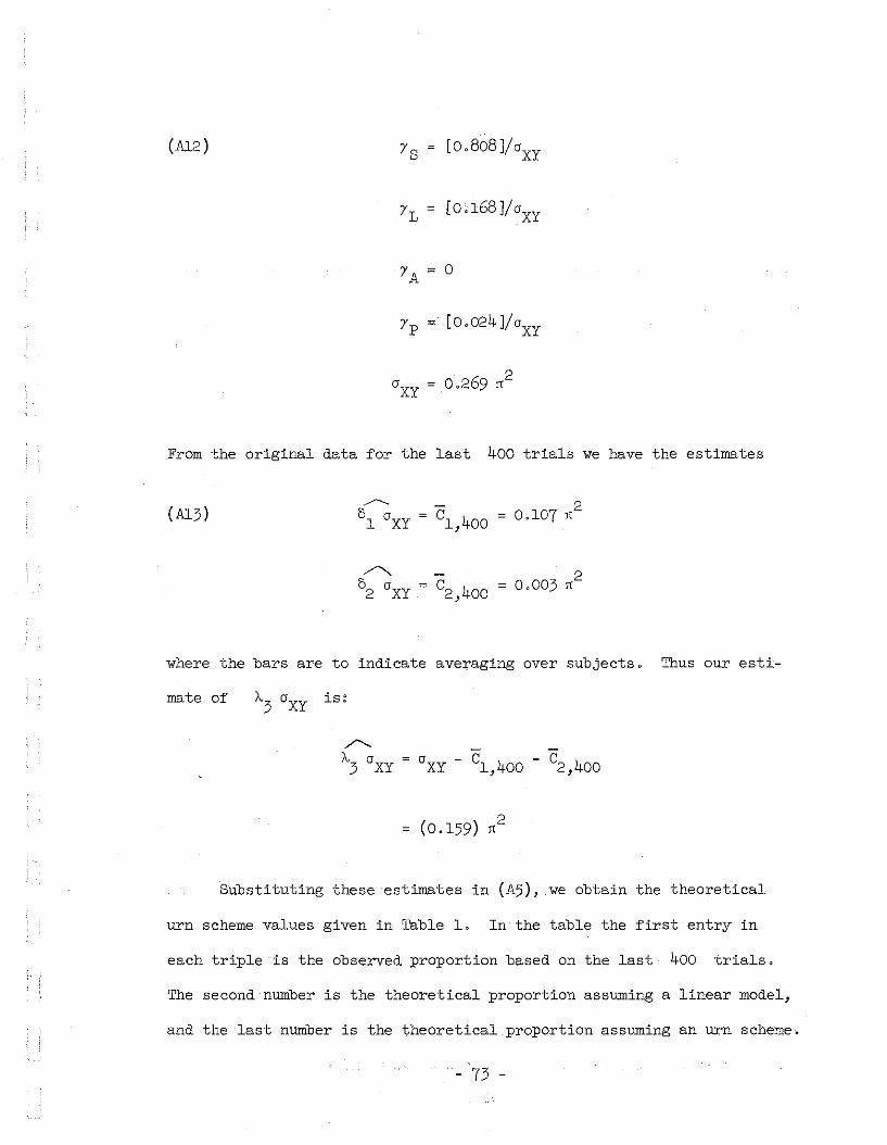
(Al2) I'S [0.808J/crXY
I'L ~ [0;168J/crXY
I'A ~ 0
I'p ~ [0.024J/crXY
crXY ~ 0.269 1(2
From the original data for the last 400 trials we have the estimates
(Al3)
~°2 crXY ~ C2,400
where the bars are to indicate averaging over subjects. Thus our esti-
mate of A.3
crXY is~
/'-
A.3 crXY crXY - Cl ,400
(0.159) 1(2
Substituting these estimates in (A5), we obtain the theoretical
urn scheme values given in Table 1. In the table the first entry in
each triple is the observed proportion based on the last 400 trials.
The second number is the theoretical proportion assuming a linear model,
and the last number is the theoretical proportion assuming an urn scheme.
- 73 -

TABLE 1
*p(xn
*= j, Yn-2 = k}
~(i,k) = S L A p
0.433 0.258 0.168 0.150s 0·550 0.345 0.291 0.299
0.478 0.224 0.157 0.167
0.419 0.277 0.148 0.151L 0.410 0.206 0.152 0.160
0.470 0.216 0.149 0.159
0.394 0.314 0.146 0.177A 0.374 0.169 0.115 0.124
0.469 0.215 0.148 0.158
0.388 0.287 0.146 0.144p 0.380 0.175 0.121 0.129
0.469 0.215 0.148 0.158
The average deviation between theoretical and observed values of the
sixteen statistics is 0.061 for the linear model and 0.037 for the
correlated urn scheme. The theoretical proportions for the linear model
were based on a minimum _X2 estimate of e (recall equation (1.9).
If we had used minimum _X2
estimates of 51 and 52 then it is clear
from a study of equations (1.6) and (1.9) that the urn scheme predictions
could be no worse than the linear model predictions. The fact that the
urn scheme predictions are better than those of the linear model even
when the former are based on the theoretically consistent estimates
(c ) does indicate that the urn scheme shows promise.i n,- 74 -
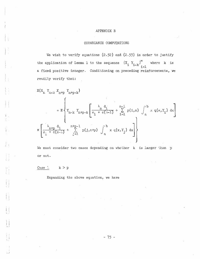
APPENDIX B
COVARIANCE COMPUTATIONS
We wish to verify eQuations (2052) and (2053) in order to justify
the appJ.ication of Lemma 1 to the seQuence [X. Y. k j'" where k is1 1- i=l
a fixed positive integer 0 Conditioning on preceding reinforcements, we
readily verify that:
E(X Y X Y )n n-k n+p n+p-k
= En-lI p(i,n)
i=l
[
AdX n+p 1 -I-
sl + c(n-l) .
n+p-lI p(j,n+p)
j=l
We must consider two cases depending on whether k is larger than p
or not.
Case 1 k>p
Expanding the above eQuation, we have
- 75 -

A d { [n-l+ n+p 1 + E Y Ysl + c(n+p-l) n-k n+p-k i~l
E(X Y x Y )n n-k n+p n+p-k
A dn 1
+ -S-l-+:-"'-C'(=-n_"""'I") I [n~-l JbE Yn- k Yn+p - k .L p(i,n+p) x q(X,Yi )
J=l a
p(i,n) Jb xa
+ E {Y k Y + k [nt p(i,n)Jb
x q(x,Y.) dx1n- n p- i=l a l J
However from Chapter 2 we know:
x[
n+p-l JbL p(j,n+p) x q(x,Y.)j=l a J
[
(n-l)A+ n
sl + c(n-l)
An fl(Y) dlsl + c{n-l)
I-An]+-c
+ [-Sl---;-A~n,--" + °ck
]+ c(n-l)
Thus, making use of the fact that the
identically distributed we find:
- 76 -
Y 'si
are independent and

COy (x Y k' X Y k)n n- n+p n+p-
\ dn 1
= -81-+"=:""CT
( n=---"'l---)
[,
(n+p-l)\_ [1-l(y)]2 c a: n+p
81
+ c(n+p-l)
glx,Y.l ax] ')l /
1 - \ J+ __n,,-+:.£pC
[\ 5 ])Y ca n+p + ~
- )J.() XY 81
+ c(n+p-l) c
[
(n-l)\ 1-\ ~ [(n+p -l)\if n + n n+p8
1+ c(n-l) -C- 8
1+ c(n+p-l)
{ [
n-l+ E Y Y
n-k n+p-k i~l
[n+
p-l Jb ~lX .L p(j,n+p) X q(X,Y.) ax
J=l a J
1 - \ ~+ n+pc
( continued)
- 77 -

2- c
2- c A 5 Jn+p k
c(n+p-l) + C
[
(n+p-l) A+ n+p
sl + c(n+p-l)
= A + B + C - D - E - F
+ 1 -C\+pl [~SlAn + 5ck1}J + c(n-l) J
where A, B, C, D, E, and F are obviously defined.
Now
" { . [ 2A 5 5 JA = +nC(~_l) [~(y) c ~ - [~(y)]2 c a]n+p +~+~
sl sl +c(n+p-l) c c
cerxy [Sl
A . :k]}- ~(y)n+p
+ c(n+p-l)
An dl ~(y) ~erXY [Sl
A+ 5p;k]n+p
sl + c( n-l) + c(n+p-l)
where we have made use of the fact that erXY = ~ - ~(Y) a. Completely
analogously we have
A dB = n+p 1
sl + c(n+p-l)
- 78 -
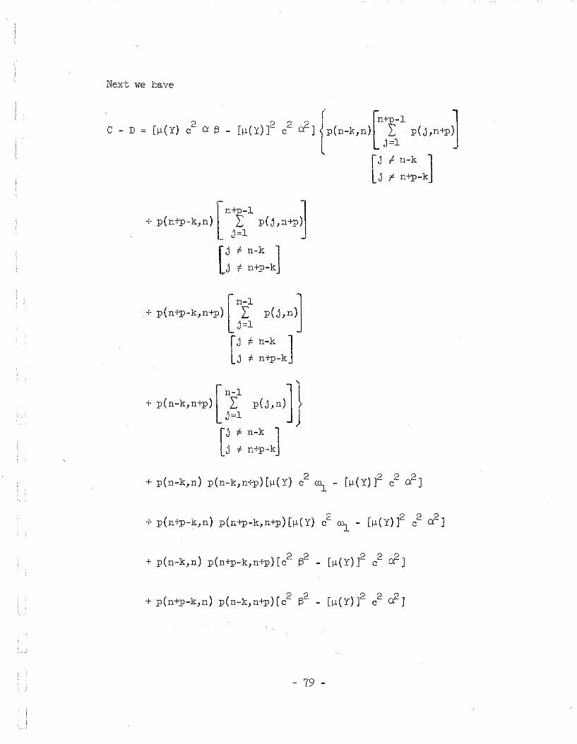
Next we have
[n+l2--1 j
+ p(n+p-k,n) ,2. p(j,n+p)J=l
[
,j F n-k ]
j # n+p-k
r n-l J+ p(n+p-k,n+p) I L p(j,n)Lj=l
[
j F n-k ]
j *' n+p-k
2 2 2 ::>+ p(n+p-k,n) p(n+p-k,n+p)[~(Y) C ill1
- [~(Y)] C 00]
2 2 2 2::>+ p(n+p-k,n) p(n-k,n+p)[c ~ - [~(Y)] c cr]
- 79 -

Where (1)1 ~ ~2 ~b Y [Jab x <;t(x,y) dx] 2 dP and its existence is
assumed,
Thus:
+ [Sl
ic o %(n+p-1)ic 1- ic ]n +~ n+p + cn+;p
+ c(n-1) . c sl + c(n+p-1)
+ [Sl
ic OJ [ (n-1)ic 1 -icn]n+p + k n +
+ c(n+p-1) ~ sl + c{n-1) c
+ [Sl
ic ok J[ (n-1)ic 1 - 'n]}n+p .£!::l2. n ++ c(n+p-1) + c s]; + c(n-1) c
+ [Sl
ic
+ :kj [Sl
ic +O~+p]n n+p+ c(n-1) + c{n+p-1)
x [",(Y) c2 2 2 if 2 a ~]~ + [",(Y)] c - 2 ",(Y) c
ic
+~] [ic 0 ]
+ [n n+p + k
sl + c(n-1) c sl + c(n+p-1) ~
x [",(Y) 2 + [r.t(y)]2 2 if - 2 r.t(Y)2 a ~]c (1)1 c c
- 80 -

Now we recall
+ [Sl
A
Ok] [Ie .
+ ;~]n n-rp+ c(n-l) + C 6
1+ c(n+p-l)
[c2 r;,2 + [i-l(Y) ]2 2 if - 2i-l(Y)2
0: illX c c
+ [Sl
Ao J[ A o Jn .~ n+p + ~+p
+ c(n-l) T c sl + c(n+p~l)
. 2 2 2 2 if _ 2i-l(Y) 2ex ill.x: [c r;, + [i-l (Y) ] c c
cov(Xn Yn- k , X Y ) = A + B + C - D - E - F and wen+p n+p-k
substitute the above values for A, Band C - D and simplify.
Thus, for k> p, we have
cov( X Y k' X Y )n n- n+p n+p-kIe 0 jn+p ~
+ c(n+p-l)" + c
2+ c
len + Ok_P]}+ c(n-l) . c
,('I 0 'n {[-Sl-+--,A'~'7(-n_-:l") + <O~_p] [s:n:p:~~~;~L + 1 - cAn+p
]
(Continued)
- 81 -

(El)
Case 2 k::; P
For k::; P analogous methods yield
Cov(X Y k' X Y )n n- n+p n+p-k+ ark]
2+ C
Equations (2.52) and (2.53) may then easily be deduced from (El) and (B2),
and the required uniformity condition is readily verified.
- 82 -

REFERENCES
Atkinson, R. C. and Estes, W. K. (1963). Stimulus sampling theory.
In Handbook of Mathematical Psychology, edited by R. D. Luce,
R. R. Bush, and E. Galanter, New York: Wiley, Vol. 2,
pp. 121-268.
Audley, R. J. and Jonckheere, A. R. (1956). The statistical analysis
of the learning process, Brit.~. Stat. Psychol., 9, pp. 87-94.
Feller, W. (1957). An Introduction to Probability Theory and its
Applications, Volume 1, second edition. New York: Wiley.
Ionescu-Tulcea, C. (1959). On a class of operators occurring in the
theory of chains of infinite order. Canadian~. Math., 11,
pp. 112-121.
Luce, R. D. (1959). Individual Choice Behavior. New York: Wiley
Norman, M. F. (1964). A Probabilistic Model for Free Responding.
Tech. Report 67 (Psychology Series). Institute for Math.
Studies in the Social Sciences, Stanford Univ., Stanford,
Calif.
Suppes, P. (1959). A linear model for a continuum of responses. In
Studies in Mathematical Learning Theory, edited by R. R. Bush
and W. K. Estes. Stanford, Calif.: Stanford University Press,
pp. 400-414.
Suppes, P. (1960). Stimulus-sampling theory for a continuum of responses.
In Mathematical Methods in the Social Sciences, 1959, edited
by K. J. Arrow, S. Karlin, and P. Suppes. Stanford, Calif.:
Stanford University Press, pp. 348-365.
- 83 -
Suppes, P. and Atkinson, R. C. (1960). Markov Learning Models for
Multiperson Interactions. Stanford, Calif.: Stanford
University Press.
Suppes, P. and Frankmann, R. W. (1961). Test of stimulus sampling
theory for a continuum of responses with unimodal non
contingent determinate reinforcement. ~. expo Psychol.,
61, 122-132.
Suppes, P. and Rouanet, H. (1964). A simple discrimination experiment
with a continuum of responses. In Studies in Mathematical
Psychology, edited by R. C. Atkinson. Stanford, Calif.:
Stanford University Press, 317-357.
Suppes, P., Rouanet, H., Levine, M., and Franllinann, R. W. (1964).
Empirical comparison of models for a continuum of responses
with noncontingent bimodal reinforcen~nt. In Studies in
Mathematical Psychology, edited by R. C. Atkinson. Stanford,
Calif.: Stanford University Press, 358-379.
Thurstone, L. L. (1930). The learning function. J. gen. Psychol., 1
469-491.
-; -. .
- 84 -
~.~ A~_'~.I .

UNCLASSIFIEDSecurity Classification
DOCUMENT CONTROL OJ.TA • R&D(Security cl4lfl4l11icatlon 01 title, body of abst,.sct lind indexlnS annotation muat be entered when thf1 o_rall report is classified)
1. O~IGIHATING ACTIVITY (Corporate author) 2a. REPORT SECURITY CLASSIFICATION
Stanford University TTn~l 000,",'; oilInstitute for Mathematical Studies in the Social 2 b. GROUP
Stanford, California Sciences~. REPORT TITLE
A Correlated Urn-Scheme for a Continuum of Responses
4. DESCRIPTIVE NOTES (Typo ot report lI11d Inc/ulIlva date")
5. AUTHOR(S) (Last narner, first name. initial)
Arnold, Barry C.
6· REPO RT DATE 7.· ':OTAI.. NO. OF PAGES \7b. NO. OF REFS
20 Julv 106s 84 11 .841. CONTRACT OR GRANT NO. ••• ORIGINATOR'!! REPORT NUMBER(S)
AF49(638)-1253b. PROJECT NO. Technical Report No. 75
c. 9778-01 9 b. OTHER RyPORT No(S) (AnY other numbera that may bo •••'snodtill. teport
d. AFOSR 65-159410. AVAILABILITY/LIMITATION NOTICES
Releasable without limitations on dissemination
11. SUPPt.. EMENTARY NOTES 12. SPONSORING MILITARY ACTIVITY
Air Force Office of Scientific ResearchAttn: SRKEWashington, D.C. 20333
13. ABSTRACTA new model to cover the case of simple learning with a continuum of responses
is presented and analysed. Called a correlated urn-scheme, it is an adaption ofthe continuous analog of the classical urn-scheme for learning. The behavior ofthe model under non-contingent reinforcement is investigated and tests of theapplicability of the model are derived. Sufficient conditions, relating to'rein-forcement schedules, for ergodic behavior in the case of contingent reinforcementare developed using a theorem due to Ionescu-Tulcea. The relation of the corre-lated urn-scheme to existing models is discussed (With much attention to the muchused linear model); and possible generalizations of the urn-scheme are suggested.An empirical comparison with the linear model is presented. The urn-scheme predict,the same asymptotic response distribution as the linear model but differs in itsprediction of se~uential dependencies. By this we mean that the urn-scheme and thelinear model predict different asymptotic response distributions conditioned onpreceding responses anajor'reinforcements. That the unconditional response distri-butiOn is in good correspondence with observation, has been verified in a number ofpapers; as has the fact that the linear model's predicted conditional distributionsare unsatisfactory. The urn-scheme shows a significant improvement in this area of~prediction, as indicated by the included empirical comparison.
DD FORM1 JAN e4 1473 UNCLASSIFIED
Security Classification

•••Security Classification
KEY WORDS
correlated urn-schemes im;ple learningdiscrete timecontinuumo~ responsesnon-contingent reinforcementcontingent rei~£orcement
ergodic behaviorsequential dependencies
INSTRUCTIONS
LINK AROL.E WT
, L.INK BI
V'lOL,E \'iT
LINKe
ROLE WT
1. ORIGINATiNG ACTIVITY: Enter the name and addressof the contractor. oubcontractor. grantee, Department of Defenee activity or other organization (corporate author) iS8uingthe report.
2•• REPORT SECURITY CLASSIFICATION: Enter the overell 0.ecuritY'clss8ification of the t$port. Indicatl8 whetherHRe15tricted Data" is included. Markins: is to be in accordance with appropriate security regulationa.
2b. GROUP: Auto.matic downgrading is specified ioDoD D1·recUve 5200.10 and Armed Forces Indu.trial Manual. Enterthe group number. Aleo. when applicable, show that optionalmarkings have been used for. Group 3 and Group 4 'as author·ized.
3. REPORT TITLE: Enter the complete report tiUe in aUcapital letters. Titles in aU cases shOUld be unclsnified.Us meaningful title cannot bSBelected without claDSification, snow title classification in all capitala in parenthesisimmediately fol1owirig the title.
4. DESCRIPTIVE NOTES: If lIlPpropriate, enter the type ofreport, e.g., interim, progl'eee, summary, annual, or final.Give the inclusive doteR when a specific reporting period iacovered.
5. AUTHOR(S): Enter the nam.e(m) of author(s)as shown onor in the report. Enter last IUlme, fust name, middle initial.If military, show rank: and branch of service. The name ofthe principal Cl.t'thor is an ab89lute minimum requirement.
6. REPORT DATE.: Enter the d.ate of the report as day,month, year, or month,. year. If more than one date appearson the report, UBe date ofpublic8tion.
7a. TOTAL NUMBER OF PAGES: The total pale countshould follow nonnal pagination procedures, i.e.,. enter thenumber of pages containing inlonnation.
7b. NUMBER OF REFERENCES: Eliter the total number ofreferences cited in the report. .
8a. CONTRACT OR GRANT NUMBER: If appropriate, enterthe applicable number of the contract or grant under whichthe report was written.
8b, Be, & Sd. PROJECT NUMBER: Enter the appropriatemilitary department identification. such as project number,subproject number, system numbera,·task number, etc.
g•. ORIGINATOR'S REPORT NUMBER(S): Ent.. the offi·cialreport'number by which the document will be identifiedand controlled by the originatina; activity. This number mustbe unique to this report.
gOb. OTHER REPORT NUMBER(S): If the report has beena8Bigned any other report numbers (either by the originatoror by the sponsor). also enter this number(s).
10. AVAILABILITY/LIMITATION NOTICES: Eet•• any 11m:itatlons on further dil!isemination of the report, other than' those
lmpoaed by security clsssification, using stQlnC/:€Ird atstementosuch as:
(1) "Qualified requesters rn.;,ly obtain COpi09 of thisreport from DOC"
(2) "Foreign announc~m<i!!ntand disaemination of thisreport by DDC iG not authorized. U
(3) "U. S. Government sgenciea may obtain copiea ofthis report directly from DDe. Other qualified DDeugers shall request through
"(4) uU. S. military ogenciee ml!y obtain copies of this
report directly from DDe. Oth~ que1ified us,-,rlBshall request through ..
(5) U All distribution of this report is controlled. Qua1~
ified DDC UBers shall request through
------------------_."If the report has been furnished to the Office of Technical
ServiceB, Department of Commerce,foT aale to the public, indigcate this fact anel enter the price, if known.
11. SUPPLEMEN1"ARY NOTES~ Uae foY additional explana..tory notes.
12. SPONSORING MILITARY ACTIVITY: Enter the name ofthe departmental project office or laboratory sponeorililg (paritll! lor) the research ODd development. Include address.
13. ABSTRACT: Enter en abstract giving a brief and factualsummary of the document indicative of the report, even thou2hit may also appear elsewhere in the body of the tech'nical re*port. If additional space is requ.ired. a continuation sheet shall 'be attached.
It is highly desirable that the abstract of c1asaified reportsbe unclassified. Each paragraph of the abstract shall end withan indication of the military security classification of the informatlott in the paragraph, represented as (TS). (5). (C), or (U)"
There is no limitation Gn the length of the abstract. However, tpe suggested length is from 150 to 225 words.
14. KEY WORDS: Key words are technically meaningful tcrmfl!or short phrases that characterize I!iI. report and may be used aaindex entries for cataloging the report. Key worda must beselected so that no security classification iIJ required. Ident!·fiers,such as equipment model designstion. trade name, militaryproject eode name, geographic location, may be used as keywords but will be followed by an indication pf technical con·text. The assignment of links, rales, and weights is optional.
DO FORM1 ..IAN 0_1 1473 (BACK) UNCLASSIFIED
Security Classification