2. Representation of Spatial Objects Ki-Joon Han Department of Computer Science & Engineering Konkuk...

2. Representation of Spatial Objects

Ki-Joon HanDepartment of Computer Science

& Engineering

Konkuk UniversityE-mail : [email protected]

URL : http://db.konkuk.ac.kr

DATABASE LAB. KONKUK UNIVERSITY 2

Introduction

This chapter Various ways of modeling and representing geometric and topological

information in GIS Euclidean space

The space of interest Rd (d=2), together with the Euclidean distance

Points Elements of the Euclidean space A pair of (Cartesian) coordinates (x,y)

Map projection A conversion to map geographic entities on a glove (hence a curved

surface) onto a planar representation Embedded space(or search space)

Region of R2 that contains the relevant objects and is bounded A sufficiently large rectangle whose edges are parallel to the axes of the

coordinate system


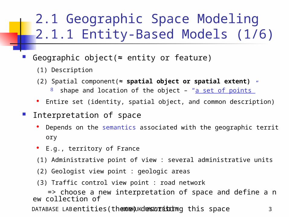
2.1 Geographic Space Modeling2.1.1 Entity-Based Models (1/6)

Geographic object(≈ entity or feature)(1) Description

(2) Spatial component(≈ spatial object or spatial extent) shape and location of the object – “a set of points”

Entire set (identity, spatial object, and common description)

Interpretation of space Depends on the semantics associated with the geographic territory E.g., territory of France

(1) Administrative point of view : several administrative units

(2) Geologist view point : geologic areas

(3) Traffic control view point : road network => choose a new interpretation of space and define a new collection of entities(theme) describing this space


2.1.1 Entity-Based Models (2/6) Types of spatial objects(1) Zero-dimensional objects or points

for representing the location of entities whose shape is not considered The area which is quite small with respect to the embedding space size E.g., cities, churches, crossings

(2) one-dimensional objects or linear objects for representing networks (roads, hydrography, and so on) Polyline

A finite set of line segments or edges, such that each segment endpoint is shared by exactly two segments

① Closed : two extreme points are identical② Simple : no pairs of nonconsecutive edges intersect at any points③ Monotone with respect to L : every line L’ orthogonal to L meets the polyline a

t one point at most


2.1.1 Entity-Based Models (3/6)

(a) line segment(edge) (b) polyline (c) non-simple polyline

(d) simple closed polyline (f) non-monotone polyline(e) monotone polyline

Figure 2.1 Examples of 1D objects


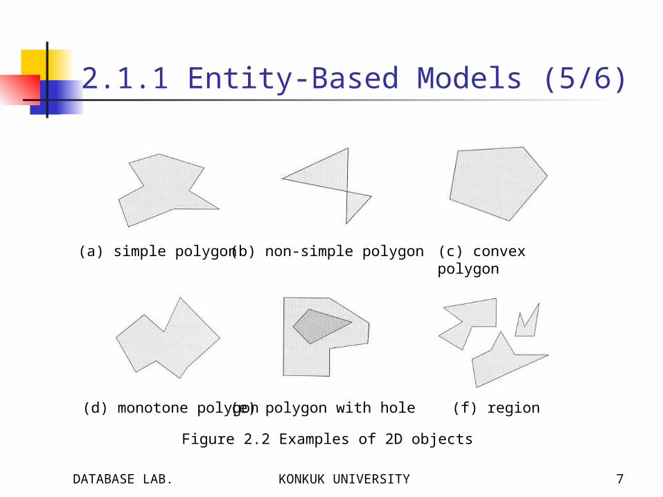
2.1.1 Entity-Based Models (4/6)(3) two-dimensional objects or surface objects

for representing entities with large areas, such as parcel or administrative units Polygon

A region of the plane bounded by a closed polyline, called its boundary① Simple : its boundary is a simple polyline② Convex : for any pair of points A and B in P the segment AB is fully included in

P③ Monotone : a simple polygon such that its boundary δP can be split into exact

ly two monotone polyline MC1 and MC2

Region A set of polygons E.g., a country and its islands


2.1.1 Entity-Based Models (5/6)

(a) simple polygon (b) non-simple polygon (c) convex polygon

(d) monotone polygon (f) region(e) polygon with hole

Figure 2.2 Examples of 2D objects


2.1.1 Entity-Based Models (6/6) Two remarks(1) The choice of geometric types is arbitrary

It depends on the future use of the collection of entities E.g., airport (scale of interest)① Point : if interested in air links② Area : if interested in the inner organization of the airport

(2) The description of linear and surfacic objects is based on line segments

We use only a linear approximation of entities in stead of higher-order polynomials in x and y

① Simplifies the design of spatial databases② Leads to efficient ways of modeling and querying spatial information Faithful approximation ≈ # of segments ≈ memory space


2.1.2 Field-Based Models Each point in space

Associated one or several attribute values(e.g., precipitation, temperature, and pollution), defined as continuous functions in x and y

E.g., altitude above sea level An example of function defined over x and y, whose result is the

value of a variable h for any point in the 2D space

Comparison(1) Field-based models

View space as a continuous field

(2) Entity-based models Identify a set of points (region, line) as an entity or object


2.2 Representation Modes Representation of infinite point sets of the Euclidean space(1) Tessellation mode

By approximating the continuous space by a discrete one E.g., city

A set of cells that cover the city’s interior

(2) Vector mode and half-plane representation By constructing appropriate data structures E.g., city

A list of points describing the boundary of a polygon


2.2.1 Tessellation (1/5) Tessellation mode(discrete model, spatial resolution model, tiling,

meshes) Decomposition of the plane(grid or raster) into disjoint cells(1) Fixed(regular) tessellation mode

Use polygonal units of equal size

(a) grid squares (square cells) (b) hexagonal cells

Figure 2.3 Regular tessellations


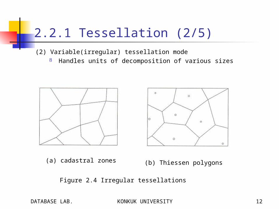
2.2.1 Tessellation (2/5)(2) Variable(irregular) tessellation mode

Handles units of decomposition of various sizes

(a) cadastral zones (b) Thiessen polygons

Figure 2.4 Irregular tessellations


2.2.1 Tessellation (3/5) Raster representation

The rectangular 2D space is partitioned into a finite number of elementary cells (NxM) (i.e., rectangular cell ≈ pixels)

A pixel has an address in the space, (x,y) where x≤ N, y≤ M

Field-based data in tessellation mode represented as a function from space

(1) Regular tessellation In applications that process image data coming from remote sensing (satellite ima

ge), such as weather or pollution forecast Domain : a finite set of pixels, as a discrete one Range : temperature or elevation

(2) Irregular tessellation In zoning (a typical GIS function) in social, demographic, or economic data Surface modeling using triangles or administrative and political units


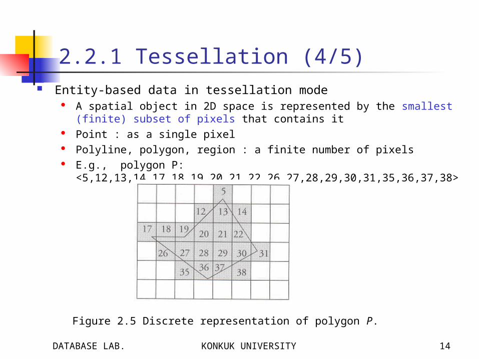
2.2.1 Tessellation (4/5) Entity-based data in tessellation mode

A spatial object in 2D space is represented by the smallest (finite) subset of pixels that contains it

Point : as a single pixel Polyline, polygon, region : a finite number of pixels E.g., polygon P:

<5,12,13,14,17,18,19,20,21,22,26,27,28,29,30,31,35,36,37,38>

Figure 2.5 Discrete representation of polygon P.


2.2.1 Tessellation (5/5) Tessellation mode

Approximate a spatial object by a finite number of cells Faithful object representation

Occupy much memory space and operate more time consuming


2.2.2 Vector Mode (1/6) Objects

Constructed from points and edges as primitives (less memory)(1) Point : represented by its pair of coordinates(2) Linear and surface objects : represented by structures(lists, sets, arrays)

on the point representation(3) Polygon : represented by the finite set of its vertices

Entity-based data in vector mode Polyline

Represented by a list of points <p1, …,pn>, each pi being a vertex Polygon

Represented as a list of points Closed polyline, i.e., (pn,p1) : edge of the polygon

Region Represented as a set of polygons


2.2.2 Vector Mode (2/6) Structure notation

[ ] : tuple < >: list { } : set

point : [x:real, y:real] polyline : <point> polygon : <point> region : {polygon}

E.g., polygon P <[4,4],[6,1],[3,0],[0,2],[2,2]>

Figure 2.6 Vector representation of polygon P


2.2.2 Vector Mode (3/6) E.g., polylines (“vertex notation”)

L1 = <1,2,3> L2 = <4,5,6,7,8,9,10,11,12> : non-simple L3 = {<13,14,19>,<15,16,19>,<17,18,19>} : a set of polylines

(a) L1 (b) L2 (c) L3

Figure 2.7 Examples of polylines


2.2.2 Vector Mode (4/6) E.g., surfacic objects (polygons and regions)

R1 = {<5,6,12,10,11>,<6,7,8,9,10,12>} : P2 and P3

R2 = {<13,14,15,16>} : P4

R3 = {<1,2,3,4>} : P1

=> concise representation compared to the rater mode

Figure 2.8 Examples of polygons


2.2.2 Vector Mode (5/6) No way to distinguish

A simple polygon from a non-simple one A convex polygon from a nonconvex one A polygon from a polyline A set of adjacent polygons from a set of disjoint or intersecting ones

Field-based data in vector mode Digital Elevation Models (DEMs)

A digital (and thereby finite) representation of an abstract modeling of space

for any natural phenomenon that is a continuous function of the 2D space (temperature, pressure, moisture, or slope)

Based on a finite collection of sample values (not all points in 2D space)=> Values at other points are obtained by interpolation (e.g., TIN)


2.2.2 Vector Mode (6/6) TIN (Triangulated Irregular Networks)

Based on a triangular partition of 2D space The elevation value is recorded at each vertex, and inferred at any other

point P by linear interpolation of the three vertices of the triangle that contains P

(a) point sample (b) triangulation (c) TIN

Figure 2.9 Progression of a triangulated irregular network (TIN)


2.2.3 Half-Plane Representation (1/4) Spatial objects

Defined with a single primitive; namely, half-planes H: half-space in the d-dimensional space RRd

The set of points P(x1,x2,…,xd) that satisfy a1x1+a2x2+…+adxd +ad+1 ≤ 0 P: convex d-dimensional polytope

The intersection of some finite number of closed half-spaces Face of P

H ∩ P, where H is part of the half-spaces defining P Q : d-dimensional polyhedron in RRd

The union of a finite number of polytopes Not necessarily convex Divide the space into its interior, its boundary, and its exterior Its components are not necessarily connected and may overlap


2.2.3 Half-Plane Representation (2/4) Convex polygon with n edges (n vertices)

The intersection of n half-planes delimited by lines Region

A union of convex polygons Line segment

The intersection of two half-lines or rays Polyline

The union of some number of line segments Point

A zero-dimensional polytope A set of points

A zero-dimensional polyhedron

=> regions, polylines, and points : polyhedra of respective dimensions 2, 1, and 0.


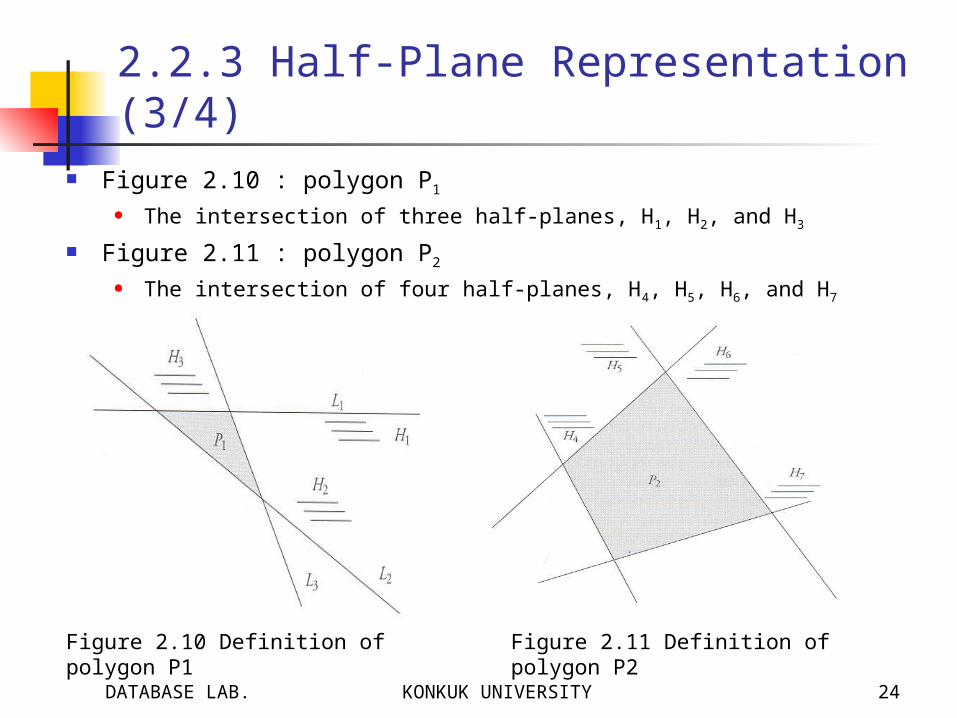
2.2.3 Half-Plane Representation (3/4) Figure 2.10 : polygon P1

The intersection of three half-planes, H1, H2, and H3

Figure 2.11 : polygon P2

The intersection of four half-planes, H4, H5, H6, and H7

Figure 2.10 Definition of polygon P1

Figure 2.11 Definition of polygon P2


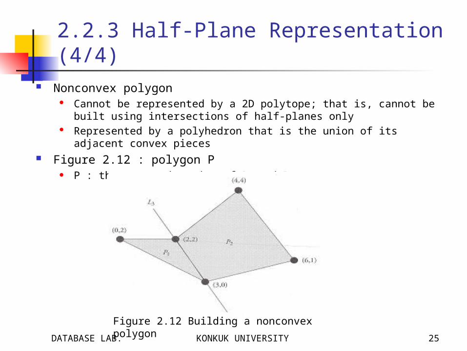
2.2.3 Half-Plane Representation (4/4) Nonconvex polygon

Cannot be represented by a 2D polytope; that is, cannot be built using intersections of half-planes only

Represented by a polyhedron that is the union of its adjacent convex pieces

Figure 2.12 : polygon P P : the geometric union of P1 and P2

Figure 2.12 Building a nonconvex polygon


2.3 Representing the Geometry of a Collection of Objects

Three representations of collections of spatial objects(1) Spaghetti model(2) Network model differ in the expression of topological

relationships(3) Topological model

Topological relationships Relations that are invariant under topological transformations Preserved when the spatial objects are translated, rotated, or scaled in

the Euclidean plane Adjacent, overlapping, disjointness, and inclusion => helpful for query evaluation


2.3.1 Spaghetti Model Spaghetti Model

The geometry of any spatial object of the collection is described independently of other objects

No topology is stored, and all topological relationships must be computed on demand

Enable the heterogeneous representation that would mix points, polylines, and regions with no restrictions

Advantage Simplicity Easy input of new objects into the collection

Drawback Lack of explicit information about the topological relationships Some representation redundancy (boundary of two adjacent regions)

Tend to large data Risk of inconsistency


2.3.2 Network Model (1/3) Network model

for representing networks in network (graph)-based applications such as transportation services or utility management (electricity, telephone, and so on)

Topological relationships among points and polylines are stored Two new concepts(1) Node

A distinguished point that connects a list of arcs -> line connectivity(2) Arc

A polyline that starts at a node and ends at a node

Two types of points (1) Node

Either an arc endpoint(extreme) or an isolated point in the plane

(2) Regular point Other line and polygon vertices


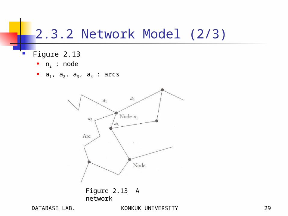
2.3.2 Network Model (2/3) Figure 2.13

ni : node a1, a2, a3, a4 : arcs

Figure 2.13 A network


2.3.2 Network Model (3/3) Network types (1) planar network

Each edge intersection is recorded as a node even though the node does not correspond to a geographic object (i.e., entity in real world)

(2) nonplanar network Edges may cross without producing an intersection E.g., ground transportation with tunnels and passes

Objects in the network model point : [x:real, y:real] node : [point, <arc>] arc: [node-start, node-end, <point>] polygon: <point> region : {polygon}=> No information on the relationships between 2D objects is

stored


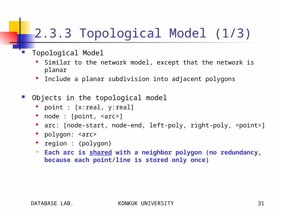
2.3.3 Topological Model (1/3) Topological Model

Similar to the network model, except that the network is planar Include a planar subdivision into adjacent polygons

Objects in the topological model point : [x:real, y:real] node : [point, <arc>] arc: [node-start, node-end, left-poly, right-poly, <point>] polygon: <arc> region : {polygon} Each arc is shared with a neighbor polygon (no redundancy,

because each point/line is stored only once)


2.3.3 Topological Model (2/3) E.g., Figure 2.14

P1 : <a, b, f> P2 : <c, d, e, f> N1 : [[3, 0], <a, f, e>] f : [N1, N2, P1, P2, <>]

Figure 2.14 Representation of polygons in the topological model


2.3.3 Topological Model (3/3) Advantage

The efficient computation of topological queries Easy consistency maintenance and updates

Drawback Some spatial objects may have no semantics in a real-world application (∵ planar) The complexity of the resulting structure may slow down some

operations (e.g., input of a new object)


2.4 Spatial Data Formats and Exchange Standard

Standard types (1) de facto (in fact) standard : 사실 표준

So dominant that everybody seems to follow it like an authorized standard

E.g., mile

(2) de jure (by law) standard : 공식 표준 Standard authorized by standardization organization such as ISO E.g., meter

DXF format As a data transfer format between CAD software data and become a

popular GIS data format Comparison criterion between spatial data formats

The richness of their underlying spatial model


2.4.1 Overview of Current Spatial Data Formats (1/2)

Official organization (1) National Institutes of standards

ANSI (American National Standards Institute) AFNOR (Association Française de Normalisation) BSI (British Standard Institute)

(2) International Organization ISO (International Organization for Standardization) DCWIG (Digital Geographic Information Working Group)

de facto standards DXF : for CAD/CAM applications (from AutoCAD) DIGEST : for military applications within many NATO countries (by

DCWIG) SDTS : used by many U.S. national agencies (by USGS)


2.4.1 Overview of Current Spatial Data Formats (2/2)

Proprietary formats France : EDIGéO format (by AFNOR) Germany : ALK/ATKIS format Switzerland : INTERLIS format United kingdom : NTF format Canada : SAIF format Korea : NGI format

=> allow the description and transfer of raster and vector data => OGC’s GML Standards for discrete (raster) representation

GIF (Graphics Interchange Format) JPEG (Joint Photographic Experts Group) TIFF (Tagged Image File Format) : most widely used for spatial data CGM (Computer Graphic Metafile) ASRP (Arc Standard Raster Product)


2.4.2 The TIGER/Line Data Format (1/7)

TIGER (Topologically Integrated Geographic Encoding and Referencing)

The name for the system and digital database developed at the U.S. Census Bureau

A practical implementation of the topological data model

TIGER/Line file A database of geographic entities such as roads, railroads, rivers, lakes,

political boundaries, and census statistical boundaries Contains the location in latitude and longitude, the name, the type of

feature (≈object), address ranges for most streets, geographic relationships to other features, and other related information

Topological structure of the TIGER database Define the location and relationships of streets, rivers, railroads, and other

features to each other and to the numerous geographic entities Designed to ensure no duplications of these features and areas



Spatial objects Belong to the Geometry and Topology (GT) class of SDTS Embody both geometry (coordinate locations and shape) and topology All spatial objects are mixed in a single layer that includes roads,

hydrography, railroads, boundary lines, and miscellaneous features Introduce many spatial objects that do not correspond to geographic

objects



Spatial object types (1) Node

0-D object that is a topological junction of two or more links or chains, or an endpoint of a link or chain

(2) Entity point A point used for identifying the location of point features such as

towers, buildings, or places

(3) Chain (≈arc) A simple polyline described by a start node, an end node, and a list of

intermediate points called shape points Intersect each other only at nodes① Complete chain

Explicitly references left and right polygons and start and end nodes

② Network chain Do not reference left and right polygons (above network model)

(4) GT-polygon An area described by the list of complete chains that form its boundary



An example of TIGER object GT-polygon : 3 Polygon interior point : for computing distances

Figure 2.15 TIGER objects (after TIGER documentation)



Extracting the representation of spatial objects from the TIGER files (1) Record type 1

TLID(TIGER/Line ID), and its start and end nodes

(2) Record type 2 The shape points of the chains up to 10 points

Table 2.1 Examples of record type 1 (chains)

Table 2.2 Examples of record type 2 (shape points)



Construction of GT-polygons (1) Record type I

Give the identifiers of the left and right polygons (CENID, POLYID)

(2) Record type 7 Contains all landmarks, together with their point coordinates and some descriptive

attributes

Table 2.3 Examples of record type I (link chains/polygons)

Table 2.4 Examples of record type 7 (landmarks)



Major types of features (1) Line features

Roads Railroads Hydrography Transportation features, power lines, and pipelines Boundaries

(2) Landmark features Point landmarks (e.g., schools and churches) Area landmarks (e.g., parks and cemeteries) Office buildings and factories

(3) Polygon features Census statistical areas School districts Voting districts Administrative divisions: states, counties, county subdivisions Blocks


2.4.3 Recent Standardization Initiatives (1/5)

Standardization of exchange formats and spatial data models for improving interoperability between GISs

OpenGIS Consortium (OGC) Created in 1994 to foster communication among GISs in order to ensure interopera

bility Dedicated to the creation and management of an industry-wide architecture for inter

operable geoprocessing

Technical goals of OGC (1) a universal spatio-temporal data and process model : OGC data model

Main entity : feature which has a type and a geometry

(2) a specification for each of the major database languages to implement the OGC data model

(3) a specification for each of the major distributed computing environments (DCEs) to implement the OGC process model



OGC’s technical activities (1) the development of an abstract specification

Create and document a conceptual model sufficient to allow for the creation of implementation specifications

① Essential model Establish the conceptual linkage of the software to the real world

② Abstract model Define the eventual software system in an implementation-neutral

manner

(2) the development of an implementation specification Technical specifications implementing the abstract requirements :

CORBA, DCOM, Java

(3) the specification revision process => formalism for all models : UML



ISO Technical Committee 211 (TC/211) : Geographic Information/Geomatics

Global standardization issues related GIS Preparing a family of geographic information standards in cooperation

with other ISO technical committees Study the standards to specify methods, tools, and services for data

management and transfer between different users, systems, and locations

Groups of TC/211 committee Working group 1 : Framework and reference model Working group 2 : Geospatial data models and operators Working group 3 : Geospatial data administration Working group 4 : Geospatial services Working group 5 : Profiles and functional standards

=> since 1997, OGC and ISO seek to converge toward a common solution

(i.e., interoperability in geospatial data processing)



Open Geospatial Datastore Interface (OGDI) To offer a solution that leverages and accelerates standardization efforts API that resides between an application and various geodata products in

order to provide standardized geospatial access methods A client/server architecture for delivering spatial data over the Internet To implement a simple feature interface for Java in OGDI as soon as

OpenGIS issues the specifications

Geodata integration needs of OGDI The distribution of geodata products via the Internet/Intranet Access to data in native format The adjustment of coordinate systems and cartographic projections The retrieval of geometric and alphanumeric data



Current map server Usually transfer GIF, JPEG, etc. Use HTTP, which is based on a stateless connection

OGDI server Use GLPT (Geographic Library Transfer Protocol)

new Internet protocol for the transfer of geospatial data A statefull replacement for HTTP

2. Representation of Spatial Objects Ki-Joon Han Department of Computer Science & Engineering Konkuk...

Documents

Transcript of 2. Representation of Spatial Objects Ki-Joon Han Department of Computer Science & Engineering Konkuk...