2 Reduced Forms VARs

2.1 Representations

The Vector Autoregressive (VAR) Representation

If the MA matrix of lag polynomials is invertible, then a unique VAR exists.

We define C(L)−1 as an (n × n) lag polynomial such that C(L)−1C(L) = I; i.e. when these

lag polynomial matrices are matrix-multiplied, all the lag terms cancel out. This operation

in effect converts lags of the errors into lags of the vector of dependent variables.

Thus we move from MA coefficient to VAR coefficients.

Define A(L) = C(L)−1. Then given the (invertible) MA coefficients, it is easy to map these

into the VAR coefficients:

Yt = C(L)εt

A(L)Yt = εt (3)

where A(L) = A0L0 +A1L1 +A2L2 + ... and Aj for all j are (n× n) matrices of coefficients.

To show that this matrix lag polynomial exists and how it maps into the coefficients in C(L),

note that by assumption we have the identity

(A0L0 +A1L

1 +A2L2 + ...)(C0L

0 + C1L1 + C2L

2 + ...) = I

After distributing, the identity implies that coefficients on the lag operators must be zero,

which implies the following recursive solution for the VAR coefficients:

A0 = I

A1 = −A0C1

Ak = −A0Ck −A1Ck−1 − ...−Ak−1C1

As noted, the VAR is possibly of infinite order (i.e. infinite number of lags required to fully

represent joint density). In practice, the VAR is usually restricted for estimation by truncating

the lag-length.

The pth-order vector autoregression, denoted VAR(p) is given by

Yt = A1Yt−1 +A2Yt−2 + ...+ApYt−p + εt (4)

Note: Here we are considering zero mean processes. In case the mean of Yt is not zero we

should add a constant in the VAR equations.

Alternative representations: VAR(1) Any VAR(p) can be rewritten as a VAR(1). To

form a VAR(1) from the general model we define: e′t = [ε′,0, ...,0], Y′t = [Y ′t , Y′t−1, ..., Y

′t−p+1]

A =

A1 A2 ... Ap−1 Ap

In 0 ... 0 0

0 In ... 0 0... . . . ...

0 ... ... In 0

Therefore we can rewrite the VAR(p) as a VAR(1)

Yt = AYt−1 + et

This is also known as the companion form of the VAR(p)

An Example: Suppose n = 2 and p = 2. The VAR will be(y1t

y2t

)=(a1

11 a112

a121 a1

22

)(y1t−1

y2t−1

)+(a2

11 a212

a221 a2

22

)(y1t−2

x2t−2

)+(ε1t

ε1t

)We can rewrite the above model as y1t

y2t

y1t−1

y2t−1

=

a111 a1

12 a211 a2

12

a121 a1

22 a221 a2

22

1 0 0 0

0 1 0 0

y1t−1

y2t−1

y1t−2

x2t−2

+

ε1t

ε1t

0

0

Setting

Yt =

y1t

y2t

y1t−1

y2t−1

, A =

a111 a1

12 a211 a2

12

a121 a1

22 a221 a2

22

1 0 0 0

0 1 0 0

, et =

ε1t

ε1t

0

0

we obtain the previous VAR(1) representation.

SUR representation The VAR(p) can be stacked as

Y = XΓ + u

where X = [X1, ..., XT ]′, Xt = [Y ′t−1, Y′t−2..., Y

′t−p]

′ Y = [Y1, ..., YT ]′, u = [ε1, ..., εT ]′ and Γ =

[A1, ..., Ap]′

Vec representation Let vec denote the stacking columns operator, i.e X =

(X11 X12

X21 X22

X31 X32

)

then vec(X) =

X11

X21

X31

X12

X22

X32

Let γ = vec(Γ), then the VAR can be rewritten as

Yt = (In ⊗X ′t)γ + εt

Stationarity of a VAR

Stability and stationarity Consider the VAR(1)

Yt = µ+AYt−1 + εt

Substituting backward we obtain

Yt = µ+AYt−1 + εt

= µ+A(µ+AYt−2 + εt−1) + εt

= (I +A)µ+A2Yt−2 +Aεt−1 + εt...

Yt = (I +A+ ...+Aj)µ+AjYt−j +

j−1∑i=0

Aiεt−i

If all the eigenvalues of A are smaller than one in modulus then

1. Aj = PΛjP−1 → 0.

2. the sequence Ai, i = 0,1, ... is absolutely summable.

3. the infinite sum∑j−1

i=0Aiεt−i exists in mean square (see e.g. proposition C.10L);

4. (I +A+ ...+Aj)µ→ (I −A)−1 and Aj → 0 as j goes to infinity.

Therefore if the eigenvalues are smaller than one in modulus then Yt has the following

representation

Yt = (I −A)−1 +

∞∑i=0

Aiεt−i

Note that the eigenvalues (λ) of A satisfy det(Iλ − A) = 0. Therefore the eigenvalues

correspond to the reciprocal of the roots of the determinant of A(z) = I −Az.

A VAR(1) is called stable if det(I − Az) 6= 0 for |z| ≤ 1. Equivalently stability requires

that all the eigenvalues of A are smaller than one in absoulte value.

A condition for stability: For a VAR(p) the stability condition also requires that all the

eigenvalues of A (the AR matrix of the companion form of Yt) are smaller than one in mod-

ulus or all the roots larger than one. Therefore we have that a VAR(p) is called stable if

det(I −A1z −A2z2, ..., Apzp) 6= 0 for |z| ≤ 1.

A condition for stationarity: A stable VAR process is stationary.

Notice that the converse is not true. An unstable process can be stationary.

Notice that the vector MA(∞) representation of a stationary VAR satisfies the absolute

summability condition so that assumptions of 10.2H hold.

Example A stationary VAR(1)

Yt = AYt−1 + εt, A =(

0.5 0.3

0.02 0.8

), Ω = E(εtε

′t) =

(1 0.3

0.3 .1

), λ =

(0.81

0.48

)

Figure 1: Blu: Y1, green Y2.

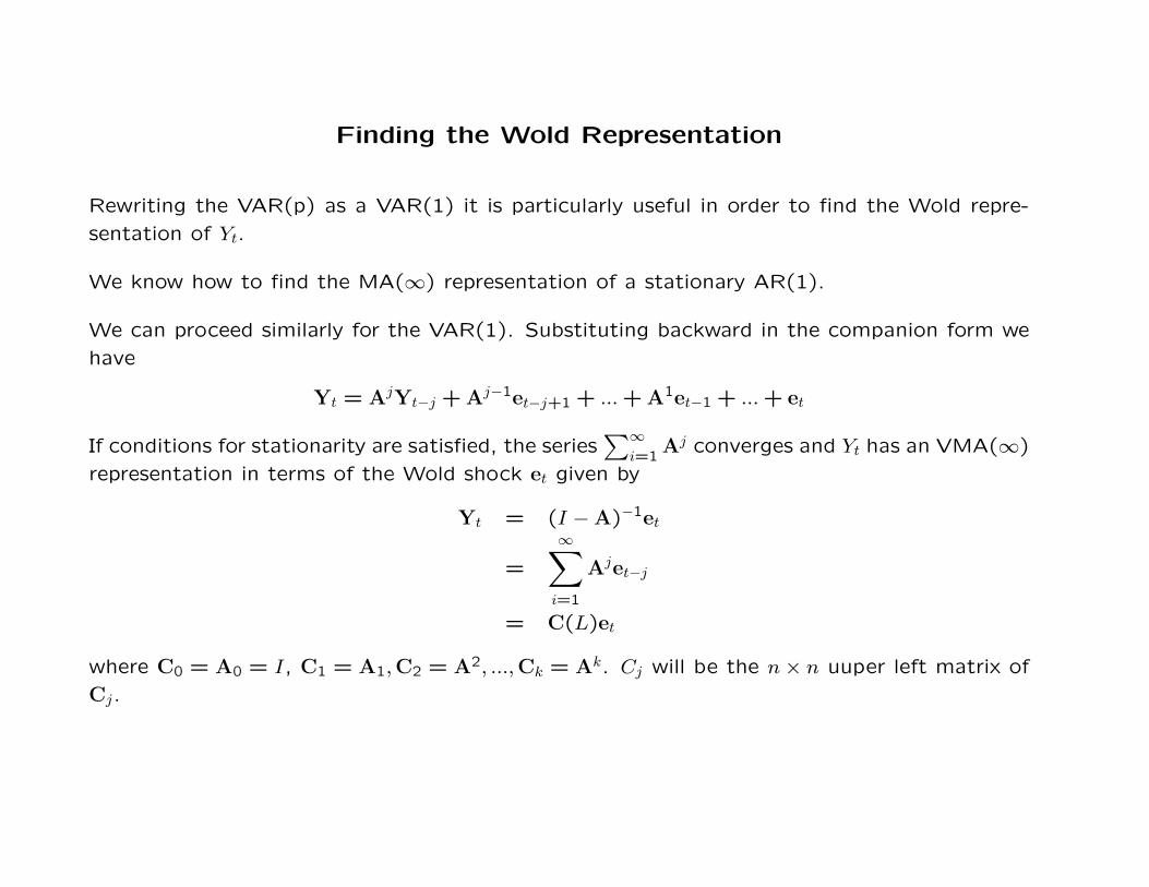
Finding the Wold Representation

Rewriting the VAR(p) as a VAR(1) it is particularly useful in order to find the Wold repre-

sentation of Yt.

We know how to find the MA(∞) representation of a stationary AR(1).

We can proceed similarly for the VAR(1). Substituting backward in the companion form we

have

Yt = AjYt−j + Aj−1et−j+1 + ...+ A1et−1 + ...+ et

If conditions for stationarity are satisfied, the series∑∞

i=1Aj converges and Yt has an VMA(∞)

representation in terms of the Wold shock et given by

Yt = (I −A)−1et

=

∞∑i=1

Ajet−j

= C(L)et

where C0 = A0 = I, C1 = A1,C2 = A2, ...,Ck = Ak. Cj will be the n× n uuper left matrix of

Cj.

Second Moments

Autocovariance of a VAR(p). Let us consider the companion form of a stationary (zero

mean for simplicity) VAR(p) defined earlier

Yt = AYt−1 + et (5)

The variance of Yt is given by

Σ = E[(Yt)(Yt)′]

= AΣA′ + Ω (6)

a closed form solution to (7) can be obtained in terms of the vec operator.

Let A,B,C be matrices such that the product ABC exists. A property of the vec operator is

that

vec(ABC) = (C ′ ⊗A)vec(C)

Applying the vec operator to both sides of (7) we have

vec(Σ) = (A⊗A)vec(Σ) + vec(Ω)

If we define A = (A⊗A) then we have

vec(Σ) = (I −A)−1vec(Ω)

The jth autocovariance of Yt (denoted Σj) can be found by post multiplying (6) by Yt−j and

taking expectations:

E(YtYt−j) = AE(YtYt−j) + E(etYt−j)

Thus

Σj = AΣj−1

or

Σj = AjΣ

The variance Σ and the jth autocovariance Σj of the original series Yt is given by the first n

rows and columns of Σ and Σj respectively.

Model specification

Specification of the VAR is key for empirical analysis. We have to decide about the following:

1. Number of lags p.

2. Which variables.

3. Type of transformations.

Number of lags As in the univariate case, care must be taken to account for all systematic

dynamics in multivariate models. In VAR models, this is usually done by choosing a sufficient

number of lags to ensure that the residuals in each of the equations are white noise.

AIC: Akaike information criterion Choosing the p that minimizes the following

AIC(p) = T ln |Ω|+ 2(n2p)

BIC: Bayesian information criterionChoosing the p that minimizes the following

BIC(p) = T ln |Ω|+ (n2p) lnT

HQ: Hannan- Quinn information criterion Choosing the p that minimizes the following

HQ(p) = T ln |Ω|+ 2(n2p) ln lnT

p obtained using BIC and HQ are consistent while with AIC it is not.

AIC overestimate the true order with positive probability and underestimate the true or-

der with zero probability.

Suppose a VAR(p) is fitted to Y1, ..., YT (Yt not necessarily stationary). In small sample

the following relations hold:

pBIC ≤ pAIC if T ≥ 8

pBIC ≤ pHQ for all T

pHQ ≤ pAIC if T ≥ 16

Type of variables Variables selection is a key step in the specification of the model.

VAR models are small scale models so usually 2 to 8 variables are used.

Variables selection depends on the particular application and in general should be included

all the variable conveying relevant information.

We will see several examples.

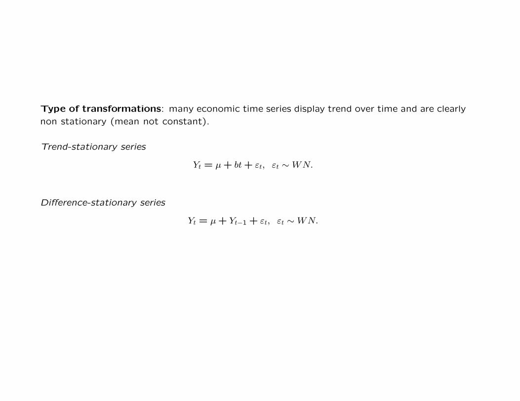
Type of transformations: many economic time series display trend over time and are clearly

non stationary (mean not constant).

Trend-stationary series

Yt = µ+ bt+ εt, εt ∼WN.

Difference-stationary series

Yt = µ+ Yt−1 + εt, εt ∼WN.

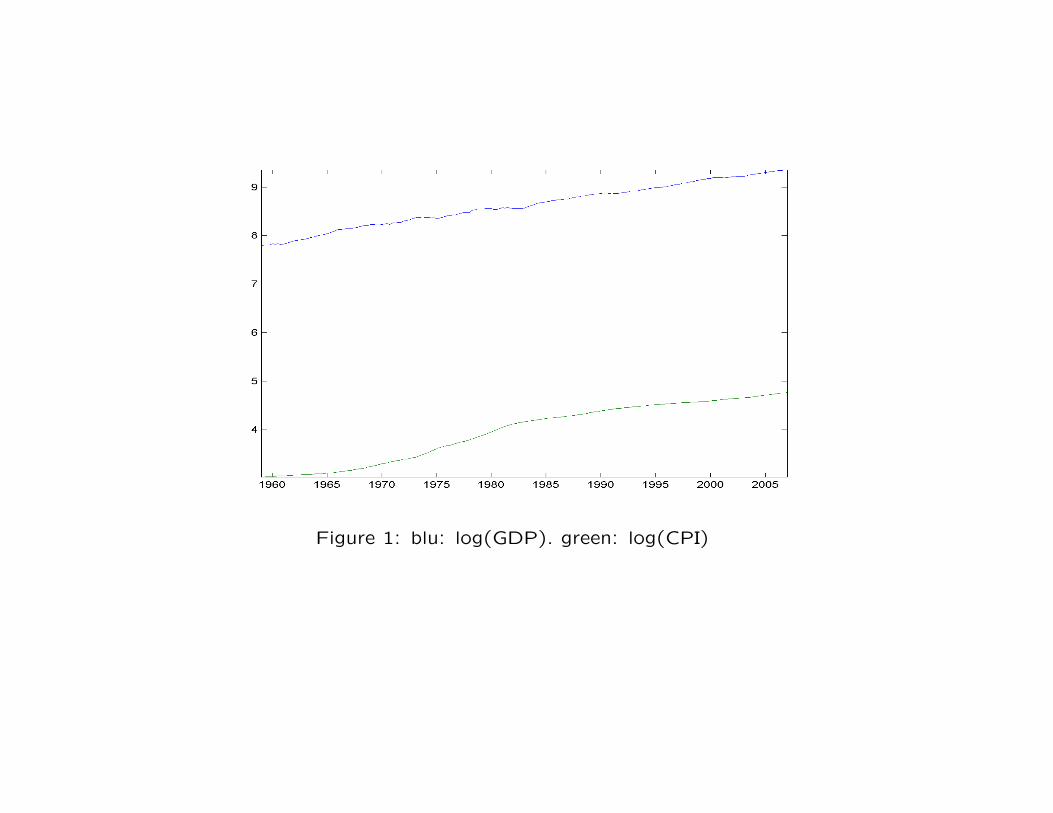
Figure 1: blu: log(GDP). green: log(CPI)

These series can be thought as generated by some nonstationary process. Here there are

some examples

Example: Difference stationary(Y1t

Y2t

)=(

0.01

0.02

)+(

0.7 0.3

−0.2 1.2

)(Y1t−1

Y2t−1

)+(ε1t

ε2t

), Ω =

(1 0.3

0.3 .1

), λ =

(1

0.9

)

Example: Trend stationary(Y1t

Y2t

)=(

0

0.01

)t+(

0.5 0.3

0.02 0.8

)(Y1t−1

Y2t−1

)+(ε1t

ε2t

)Ω =

(1 0.3

0.3 .1

), λ =

(0.81

0.48

)

So:

1) How do I know whether the series are stationary?

2) What to do if they are non stationary?

Dickey-Fuller test In 1979, Dickey and Fuller have proposed the following test for station-

arity

1. Estimate with OLS the following equation

∆xt = b+ γxt + εt

2. Test the null γ = 0 against the alternative γ < 0.

3. If the null is not rejected then

xt = b+ xt + εt

which is a random walk with drift.

4. On the contrary if γt < 0, then xt is a stationary AR

xt = b+ axt + εt

with a = 1 + γ < 1.

An alternative is to specify the equation augmented by a deterministic trend

∆xt = b+ γxt + ct+ εt

With this specification under the alternative the preocess is stationary with a deterministic

linear trend.

Augmented Dickey-Fuller test. In the augmented version of the test p lags of the lags of

∆xt can be added, i.e.

A(L)∆xt = b+ γxt + εt

or

A(L)∆xt = b+ γxt + ct+ εt

• If the test statistic is smaller than (negative) the critical value, then the null hypothesis of

unit root is rejected.

Transformations I: first differences Let ∆ = 1−L be the first differences filter, i.e. a filter

such that ∆Yt = Yt − Yt−1 and let us consider the simple case of a random walk with drift

Yt = µ+ Yt−1 + εt

where εt is WN. By applying the first differences filter (1−L) the process is transformed into

a stationary process

∆Yt = µ+ εt

Let us now consider a process with deterministic trend

Yt = µ+ δt+ εt

By differencing the process we obtain

∆Yt = δ + ∆εt

which is a stationary process but is not invertible because it contains a unit root in the MA

part.

log(GDP) and log(CPI) in first differences

Transformations II: removing deterministic trend Removing a deterministic trend (linear

or quadratic) from a process from a trend stationary variable is ok.

However this is not enough if the process is a unit root with drift. To see this consider again

the process

Yt = µ+ Yt−1 + εt

this can be writen as

Yt = µt+ Y0 +

t∑j=0

εj

By removing the deterministic trend the mean of the process becomes constant but the

variance grows over time so the process is not stationary.

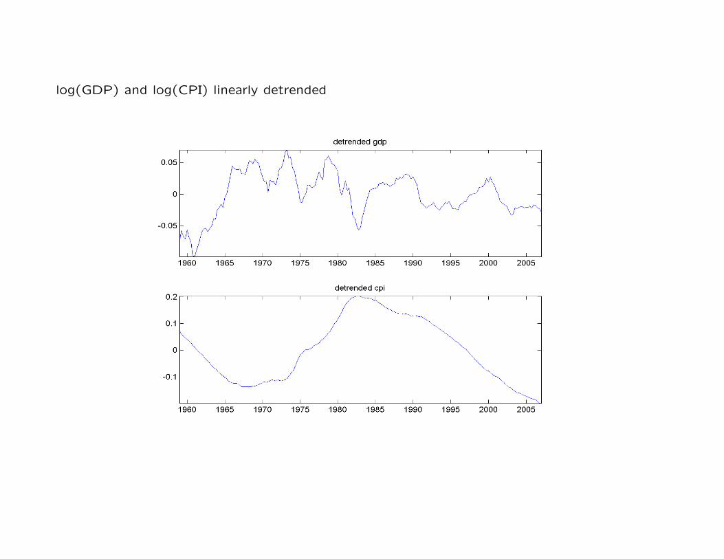
log(GDP) and log(CPI) linearly detrended

Transformations of trending variables: Hodrick-Prescott filter The filter separates the

trend from the cyclical component of a scalar time series. Suppose yt = gt + ct, where gt

is the trend component and ct is the cycle. The trend is obtained by solving the following

minimization problem

mingtTt=1

T∑t=1

c2t + λ

T−1∑t=2

[(gt+1 − gt)− (gt − gt−1)]2

The parameter λ is a positive number (quarterly data usually =1600) which penalizes vari-

ability in the growth component series while the first part is the penalty to the cyclical

component. The larger λ the smoother the trend component.