1

2 MODELS FOR BINARY OUTCOMES.........................................................................................4

2.1 INTRODUCTION ..........................................................................................................................4 2.1.1 Link functions .......................................................................................................................4 2.1.2 Methods of estimation...........................................................................................................7

2.1.2.1 MAP estimation ........................................................................................................................9 2.1.2.2 Numerical quadrature..............................................................................................................10

2.2 MODELS BASED ON A SUBSET OF THE TVSFP DATA ................................................................12 2.2.1 The data..............................................................................................................................12

2.2.1.1 Exploring the data ...................................................................................................................14 Crosstabulation .......................................................................................................................................14 Exploratory graphs..................................................................................................................................15 Univariate graphs ....................................................................................................................................17

2.2.2 A 2-level random intercept logistic model with 2 predictors..............................................19 2.2.2.1 The model ...............................................................................................................................19 2.2.2.2 Setting up the analysis.............................................................................................................21 2.2.2.3 Discussion of results................................................................................................................25

Syntax .....................................................................................................................................................25 Model and data description .....................................................................................................................26 Descriptive statistics ...............................................................................................................................27 Results for the model without any random effects ..................................................................................27 Results for the model fitted with adaptive quadrature.............................................................................28

2.2.2.4 Interpreting the adaptive quadrature results ............................................................................30 Estimated outcomes for different groups: unit-specific results ...............................................................31 Estimated outcomes for different groups: population-average results.....................................................35

2.2.2.5 Interpreting the contents of the level-2 residual file ................................................................38 2.2.3 A 2-level random intercept logistic regression model ........................................................40

2.2.3.1 Setting up the analysis.............................................................................................................40 2.2.3.2 Discussion of results................................................................................................................41

2.2.4 A 3-level random intercept logistic regression model ........................................................44 2.2.4.1 The model ...............................................................................................................................44 2.2.4.2 Setting up the analysis.............................................................................................................45 2.2.4.3 Discussion of results................................................................................................................45 2.2.4.4 Interpreting the adaptive quadrature results ............................................................................48

3-level ICCs ............................................................................................................................................48 Estimated unit-specific and population-average probabilities.................................................................49

2.3 MODELS BASED ON THE SUBSET OF NESARC DATA................................................................51 2.3.1 The data..............................................................................................................................51 2.3.2 A 2-level random intercept probit model............................................................................53

2.3.2.1 The model ...............................................................................................................................53 2.3.2.2 Setting up the analysis.............................................................................................................54 2.3.2.3 Discussion of results................................................................................................................56

Model and data description .....................................................................................................................57 Descriptive statistics ...............................................................................................................................57 Results for the model without any random effects ..................................................................................58 Results for the model with random effects..............................................................................................59

2.3.2.4 Interpreting the adaptive quadrature results ............................................................................60

2

2.3.3 A 2-level random intercept model with additional predictors ............................................62 2.3.3.1 The model ...............................................................................................................................62 2.3.3.2 Setting up the analysis.............................................................................................................62 2.3.3.3 Discussion of results................................................................................................................63

Results for the model fitted with adaptive quadrature.............................................................................63 2.3.3.4 Interpreting the adaptive quadrature results ............................................................................65

Estimated outcomes for different groups: unit-specific results ...............................................................65 Model comparison ..................................................................................................................................66

References ....................................................................................................................................................67

3

TABLE XXX.1 LINK FUNCTIONS FOR THE BERNOULLI DISTRIBUTION ..............................5

FIGURE XXX.1 CUMULATIVE DENSITY OF LINK FUNCTIONS ................................................7

TABLE XXX.2: CROSSTABULATION OF CC, TV AND THKSBIN ..............................................14

TABLE XXX.3: OBSERVED PROPORTION OF HIGH POST–INTERVENTION SCORES ......15

FIGURE XXX.2: EXPLORATORY GRAPH OF THKSBIN VS. PRETHKS...................................16

FIGURE XXX.3: BAR CHART OF PRETHKS VALUES ..................................................................18

TABLE XXX.4: MEAN PRE-INTERVENTION SCORES.................................................................19

TABLE XXX.5: ESTIMATED UNIT-SPECIFIC PROBABILITY OF A HIGH POST-INTERVENTION KNOWLEDGE SCORE ..........................................................................................33

FIGURE XXX.4: BAR CHART OF ESTIMATED UNIT-SPECIFIC PROBABILITIES ...............34

TABLE XXX.6: ESTIMATED POPULATION-AVERAGE PROBABILITIES...............................37

TABLE XXX.7: OBSERVED AND PREDICTED PROPORTIONS OF HIGH POST–INTERVENTION SCORES....................................................................................................................38

TABLE XXX.8: OBSERVED AND PREDICTED PROPORTIONS OF HIGH POST–INTERVENTION SCORES....................................................................................................................43

TABLE XXX.9: COMPARISON OF RESULTS FOR THREE MODELS WITH BINARY VARIABLE THKSBIN AS OUTCOME................................................................................................47

TABLE XXX.10: PROBABILITIES OF HAVING A DEPRESSION EPISODE..............................61

FIGURE XXX.5: EXPECTED PROBABILITIES FOR SUBGROUPS.............................................61

TABLE XXX.11: PROBABILITIES OF HAVING DEPRESSION EPISODES FOR SELECTED AGE GROUPS..........................................................................................................................................65

FIGURE XXX.6: ESTIMATED PROBABILITIES FOR SUBGROUPS...........................................66

TABLE XXX12: MODEL COMPARISON...........................................................................................66

4

2 Models for binary outcomes

2.1 Introduction

The nominal and ordinal outcome models can be seen as generalizations of the binary outcome model. In order to understand these models, an understanding of the binary outcome model is required.

A binary random variable is a discrete random variable that has only two possible values, such as whether a subject dies (event) or lives (non-event). Such events are often described as success versus failure, and coded using the values 0 or 1. Consequently, the assumption that this type of outcome variable has a normal distribution does not hold anymore.

The most common distribution used for a binary outcome is the Bernoulli distribution, which takes a value 1 with probability of success p and a value 0 with probability of failure 1q p . The selection of the distribution for the outcome variable is not fixed. For example, if the occurrence is very rare, the Poisson distribution can be used.

2.1.1 Link functions

In the case of a binary variable, observed values are usually assigned as either 0 or 1. When such a variable is treated as if it were continuous, predicted values, indicating the probability of the event occurring, can fall outside the (0,1) interval. Moreover, the assumption of normality at level 1 is not realistic as the random effects can no longer be assumed to have a normal distribution or to have homogeneous variance.

The multilevel generalized linear model (MGLM) generalizes the multilevel model for continuous outcomes by additionally allowing for error distributions from the exponential family (see, for example, McCullagh & Nelder, 1989). Let y denote the outcome variable, and ( )E y the expected value of y . The key to MGLM models

5

is that a nonlinear relationship between ( )E y and is allowed, with the aid of a link function.

Suppose that 1 nx xx is the vector of all the predictors and that 1 n â

is the vector of unknown regression parameters. In the models discussed up to now, it was assumed that the outcomes were normally distributed variables and that a model of the form

' ' , 1,2,...,ij ij ij i ij iy j n x â z v

could be used to describe the relationship between the outcome and predictor variables. The vector '

ijz denotes a design vector for the random effects contained in

the vector iv , and 'ijx is the design vector for the predictors in the fixed part of the

model with corresponding vector â of regression parameters. The covariance

matrix of iv is denoted by (2) and the variance of ij by 2 .

The link function specifies a nonlinear transformation between the linear predictor and the assumed distribution function. These link functions transform the observed outcome value to a function x â and ensure that the predicted probability lies within the (0,1) interval. Instead of y, is being analyzed. For the binary outcome, the probability of success is the predictor of interest.

The most commonly used link functions are the log, logit, probit and complementary log-log link functions. The log link generally is used for the count variable with Poisson distribution, which will be discussed in the next chapter. The link functions available in SuperMix include the logit, probit and complementary log-log functions for models with an ordinal dependent variable, and the logit link function for models with a nominal dependent variable. Table XXX.1 shows these link functions, along with their distribution functions (CDF), means and variances.

Table XXX.1 Link functions for the Bernoulli distribution

6

Link name Link function 1F p

, 0 1p

CDF w

Mean Variance

logit (logistic) logit ln1

pp

p

1

w

w

e

e 0

2

3

probit

1 ( )p , where 1 is the

inverse of the standard normal cumulative distribution

w 0 1

complementary log-log log log 1 p

1-exp exp w

-0.577 2

6

These link functions map the probability with an open interval (0,1) to the entire set of real numbers . Figure XXX.1 illustrates how a real number w is transformed to the probability .

As shown below, the logit and probit link functions are both symmetric around a value of 0. The logit function has a larger variance. The complementary log-log link function is asymmetric. When the probability of a successful outcome ( p ) is extremely small or large, the linear relationship does not hold. Understanding the nature of the link function used in an analysis is essential to the correct interpretation of the results.

7

Figure XXX.1 Cumulative density of link functions

In this chapter, we will consider examples of two- and three-level models based on two data sets, both with binary outcome variables. These data will also be used to illustrate the ordinal outcome model in Chapter XXX.

2.1.2 Methods of estimation

For models with binary, ordinal, count, and nominal outcomes, SuperMix offers two methods of estimation: maximization of the posterior distribution (MAP) and numerical integration (adaptive and non-adaptive quadrature) to obtain parameter and standard error estimates.

The MAP method of estimation can be used to obtain a point estimate of an unobserved quantity on the basis of empirical data. It is closely related to Fisher's method of maximum likelihood (ML), but employs an augmented optimization

8

objective which incorporates a prior distribution over the quantity one wants to estimate.

Quadrature is a numeric method for evaluating multi-dimensional integrals. For mixed effect models with count and categorical outcomes, the log-likelihood function is expressed as the sum of the logarithm of integrals, where the summation is over higher-level units, and the dimensionality of the integrals equals the number of random effects.

Typically, MAP estimates are used as starting values for the quadrature procedure. When the number of random effects is large, the quadrature procedures can become computationally intensive. In such cases, MAP estimation is usually selected as the final method of estimation. Numerical quadrature, as implemented in SuperMix, offers users a choice between adaptive and non-adaptive quadrature. Quadrature uses a quadrature rule, i.e., an approximation of the definite integral of a function, usually stated as a weighted sum of function values at specified points within the domain of integration.

Adaptive quadrature generally requires fewer points and weights to yield estimates of the model parameters and standard errors that are as accurate as would be obtained with more points and weights in non-adaptive quadrature. The reason for that is that the adaptive quadrature procedure uses the empirical Bayes means and covariances, updated at each iteration to essentially shift and scale the quadrature locations of each higher-level unit in order to place them under the peak of the corresponding integral.

A full description of these methods is given in Chapter XXX. A brief description of MAP estimation and quadrature follows below.

9

2.1.2.1 MAP estimation

For level-2 unit i , let 1 2, ,...,i i irv v v denote the random effects and 1 2, ,...,ni i iny y y the

outcomes. Let ,i if v y denote the joint distribution of 1 2, ,...,i i i irv v vv and

1 2, ,...,ii i i iny y yy .

Using standard results for conditional distributions, it follows that

| | / .i i i i i if f f fv y y v v y

By taking logarithms on both sides of the equation, the following density function is obtained:

ln | ln | lni i i i if f f K v y y v v

where K is a constant. Mode estimates iv of the random effects and estimates â of the fixed parameters are obtained by iteratively solving the equations

ln | 0,i i

k

f

v y

where k is a typical element of the unknown parameters 1 2, ,...,i i irv v v and

1 2, ,..., p .

As a by-product of the iterative procedure, estimates of cov , 1, 2,...,i i Nv are

obtained and these, in turn, are used to estimate 2 cov i v .

10

2.1.2.2 Numerical quadrature

Since

, |i i i i if f fy v y v v

it follows that the marginal distribution of iy can be obtained as the solution to the

multi-dimensional integral

1

1... | .... .r

i i i r

v v

f f f dv dv y y v v

Since it is assumed that (2)~ ,i Nv 0 Ö it follows, for example, that

/ 2 1/ 2 ' 1

(2) (2)

12 | | exp .

2r

i i if v Ö vÖ v

In general, a closed-form solution to this integral does not exist. To evaluate integrals of the type described above, we use a direct implementation of Gauss-Hermite quadrature (see, e.g., Krommer & Ueberhuber, 1994, Section 4.2.6 and Stroud & Sechrest, 1966, Section 1).

With this rule, an integral of the form

2( ) ( ) expI t f t t dt

is approximated by the sum

1

( ) ,Q

u uu

I t w f z

11

where uw and uz are weights and nodes of the Hermite polynomial of degree Q. A

Q-point adaptive quadrature rule is a quadrature rule constructed to yield an exact result for polynomials of degree 2 1Q , by a suitable choice of the n points ix and

n weights iw .

12

2.2 Models based on a subset of the TVSFP data

2.2.1 The data

The data are from the Television School and Family Smoking Prevention and Cessation Project (TVSFP) study (Flay, et. al., 1988). The study was designed to test the independent and combined effects of a school-based social-resistance curriculum and a television-based program in terms of tobacco use and cessation. The data from the study included a total of 1,600 students with both pre- and post-intervention scores from 135 classrooms drawn from 28 schools. Schools were randomized to one of four study conditions:

o A social-resistance classroom curriculum,

o A media (television) intervention,

o A social-resistance classroom curriculum combined with a mass-media intervention, and

o A no-treatment control group

A tobacco and health knowledge scale was used in classifying subjects as knowledgeable or not. In its original form, the student's score was defined as the number of correct answers to seven items on tobacco and health knowledge.

The structure of this study indicates a three-level hierarchical structure. However, we will first consider two two-level structures. In the first, students are nested within schools; in the second, students are nested within classrooms. Finally, a three-level model recognizing the role of both classroom and school in the hierarchical structure of the data will be considered.

Data for the first 10 participants on most of the variables used in this section are shown below in the form of a SuperMix spreadsheet file, named tvsfpors.ss3, located in the Examples\Binary subfolder.

13

The variables of interest are:

o School indicates the school a student is from (28 schools in total).

o Class identifies the classroom (135 classrooms in total).

o THKSord represents the tobacco and health knowledge scale, with 4 categories ranging between 1 and 4. The frequency distribution of the post-intervention THKS scores indicated that approximately half the students had scores of 2 or less, and half of 3 or greater. In terms of quartiles, four ordinal classifications were suggested corresponding to 0 – 1, 2, 3, and 4 – 7 correct responses.

o THKSbin is a recoded version of the ordinal variable THKSord, but in binary form: a value of "0" indicates an original scale score of 1 or 2, while a value of "1" indicates an scale score of 3 or 4. This variable will serve as our outcome variable in the current chapter.

o PreTHKS indicates a student's score prior to intervention, i.e., the number correct of 7 items.

o CC is a binary variable indicating whether a social-resistance classroom curriculum was introduced, with 0 indicating "no" and 1 "yes."

o TV is an indicator variable for the use of media (television) intervention, with a "1" indicating the use of media intervention, and "0" the absence thereof.

o CC*TV is the product of the variables TV and CC, and represents the CC by TV interaction.

14

In this chapter, we consider models for binary outcomes, using quadrature as method of estimation.

2.2.1.1 Exploring the data

Crosstabulation

The focus is on the influence of the intervention on the tobacco health knowledge scores of the students, as represented by the binary outcome variable THKSbin. A cross-tabulation of the variables CC and TV for the two categories of the binary variable THKSbin is given in Table XXX.2 below.

Table XXX.2: Crosstabulation of CC, TV and THKSbin

THKSbin CC Total 0 1 0 TV 0 246 140 386

1 215 152 367

Total 461 292 753

1 TV 0 175 240 415

1 201 231 432

Total 376 471 847

The proportion of students with high scale scores (THKSbin = 1) in each of the four cells formed by the categories of CC and TV can be derived from Table XXX.2. For example, 246 students in the category CC = 0, TV = 0 had a low score (THKSbin = 0), while 175 students had a high score (THKSbin = 1). The proportion of students in

this cell with a high score is thus 175

0.4157175 246

. The observed proportions of

high scores are summarized in Table XXX.3 below.

15

Table XXX.3: Observed proportion of high post–intervention scores

Study condition Proportion odds logits

CC = 0, TV = 0 0.4157 0.711 -0.340

CC = 0, TV = 1 0.4832 0.935 -0.067

CC = 1, TV = 0 0.6316 1.714 0.539

CC = 1, TV = 1 0.6031 1.520 0.418

Proportions less than 0.5 indicate odds less than one and negative logits, while proportions above 0.5 yield odds greater than one and positive logit values. We note that, based on the observed proportion of high post-intervention scores, the use of only the social-resistance classroom curriculum (as represented by the variable CC) seemed the most successful, followed by the use of both curriculum and media intervention (CC = 1, TV = 1).

Exploratory graphs

The pre-intervention scores of the students may be useful as a covariate in the analysis. To get an idea of the relationship between the scale score PreTHKS and the post-intervention score THKSbin, an exploratory graph is created. Select the Data-based Graphs, Exploratory option from the File menu.

The New Graph dialog box is activated. Select the binary outcome variable THKSbin as the Y variable and the pre-intervention score PreTHKS as the X variable. Uncheck the Draw points check box, which is checked by default, to obtain the settings as shown.

16

Click OK to obtain Figure XXX.2. The value associated with the tick marks on the X-axis represents the proportion of students with that PreTHKS score that had a value of 1 on the THKSbin variable, in other words the proportion of students with a post-intervention score of 3 or 4. We note that the relationship is reasonably linear, and that higher post-intervention scores are more often observed for students with high pre-intervention scores, which is what one intuitively would expect.

Figure XXX.2: Exploratory graph of THKSbin vs. PreTHKS

17

Univariate graphs

We now take a closer look at the distribution of the pre-intervention scores by utilizing the Data-based Graphs, Univariate option on the File menu. By default, a bar chart will be produced. Select the variable PreTHKS in the Plot column, and click Plot.

By clicking anywhere in the bars, the Bar Graph Parameters dialog box is activated. Click the Data button and then OK to display the data used to construct the bar chart.

18

Figure XXX.3 below shows both the graphing window with bar chart and the data in spreadsheet format. Note that only 55 of the 1600 observations showed a score of 5 or higher, and that no student obtained a post-intervention score of 7 out of 7.

Figure XXX.3: Bar chart of PreTHKS values

Finally, we also take a look at the mean pre-intervention scores of the students for each of the four subgroups. These are summarized in Table XXX.4 below, and show that the mean pre-intervention scores do not differ much.

19

Table XXX.4: Mean pre-intervention scores

Study condition Mean CC = 0, TV = 0 2.152

CC = 0, TV = 1 2.087

CC = 1, TV = 0 2.050

CC = 1, TV = 1 1.979

2.2.2 A 2-level random intercept logistic model with 2 predictors

2.2.2.1 The model

The outcome variable THKSbin used here is binary. It assumes a value of "0" when the original scale score was either 1 or 2, and a value of "1" for an original scale score of 3 or 4. The predicted value of the outcome can be viewed as the predicted probability that THKSbin is 1. As explained in Section 2.1.1, predicted values outside the interval [0,1] would not be meaningful and a model constraining predicted values to lie in this interval would be appropriate, in contrast with the model for a continuous outcome (see above) where effect sizes outside this interval would be interpretable. In addition, the assumption of normality at level 1 is not realistic, as the level-1 random effect can only assume one of two values: 0 or 1. This random effect can thus not have homogeneous variance.

In order to insure that the predicted values lie within the (0,1) interval, a transformation of the level-1 predicted probability can be used. For the binary case considered here, the following link function is used:

Prob(THKSbin 1| , )1

ij

ijij

e

e

â v

where ij represents the log of the odds of success.

20

For the current model, we want to explore the relationship between the post-intervention scores and the type of intervention applied. This relationship can be expressed as

Level 1 model:

0 1 2 3 4CC TV CC *TV PreTHKSij i i i i i i i ij i ij ijb b b b b e

Level 2 model:

0 0 0

1 1

2 2

3 3

4 4

i i

i

i

i

i

b v

b

b

b

b

An equivalent expression for the model is

0 1 2 3 4 0CC TV CC *TV PreTHKS .ij i i i ij ij i ijv e

21

The interpretation of the logistic regression model is made in terms of the logits, as the model is linear in terms of the logits. Thus the coefficients 1 2 4, , , can be

interpreted as follows:

o 0 is the THKS logit for CC = 0, TV = 0, that is the log odds of a positive

outcome for an individual from the control group where no intervention was made and with a pre-intervention score of 0. One could also refer to 0 as

the PreTHKS adjusted logit for the CC = 0, TV = 0 subgroup.

o 1 = the logit difference between (CC = 1, TV = 0) and (CC = 0, TV = 0) for

the case where PreTHKS = 0:

0 1 3 2 4 0( TV )CC TV PreTHKSij i i i ij iv ,

in other words, the PreTHKS adjusted logit difference between these two subgroups.

o 2 = the logit difference between (TV = 1, CC = 0) and (TV = 0, CC = 0) with

PreTHKS = 0:

0 2 3 1 4 0( CC )TV CC PreTHKSij i i i ij iv .

o 3 is the difference in logit attributable to the interaction between the two

intervention methods.

The interpretation of the coefficients is dependent on the coding of the variables used in the model.

2.2.2.2 Setting up the analysis

Using the data in tvsfpors.ss3, we consider the situation where students are nested within schools, and fit a two-level model with the binary variable THKSbin as outcome. We wish to examine the relationships between the outcome and the two intervention methods employed, simultaneously taking students' pre-intervention scores into account. To do so, we use the model described above with schools as the level-2 units.

22

Use the File, Open Spreadsheet option to activate the Open dialog box. Browse for the file tvsfpors.ss3 in the Examples\Binary folder. Select the file and click the Open button to return to the main SuperMix window, where the contents of the SuperMix system file are displayed.

Next, we use the SuperMix interface to provide the model specifications. From the main menu bar, select the File, New Model Setup option.

The Model Setup dialog box that appears has six tabs: Configuration, Variables, Starting Values, Patterns, Advanced, and Linear Transforms. In this example, only three of the tabs are used.

As a first step, the binary outcome variable THKSbin is selected from the Dependent Variable drop-down list box. The type of outcome is specified as binary using the drop-down list box in the Dependent Variable Type field. Once this selection is made, the Categories field is displayed. The school identification variable is used to define the hierarchical structure of the data, and is selected as the Level-2 ID from the Level-2 IDs drop-down list box. A title for the analysis (optional) is entered in the Title fields. A convergence criterion of 0.0001 is requested. By default, the maximum number of iterations performed is set to 100. Empirical Bayes residuals, written to additional output files, are requested by setting the Write Bayes Estimates option to means and (co)variances. Default settings for all other options associated with this tab are used. Proceed to the Variables tab by clicking on this tab.

23

The Variables tab is used to specify the fixed and random effects to be included in the model. Start by selecting the explanatory (fixed) variables using the first column of boxes in the Available group field. The first variable selected is PreTHKS, followed by CC, TV, and the interaction term CC*TV. After selecting these explanatory variables, the random effect(s) at level 2 must be selected. In this case, we wish to allow only the intercept to vary randomly over the schools. By default, the intercept is assumed to vary randomly over higher levels of the hierarchy as indicated by the checked box for the Include Intercept option in the L-2 Random Effects group field. A common fixed intercept coefficient is also included, as shown in the Explanatory Variables group field.

24

We opt to increase the number of quadrature points to be used during estimation. To do so, click the Advanced tab. First select adaptive quadrature from the Optimization Method drop-down list box, then change the Number of Quadrature Points field to 25. The default distribution for a binary outcome variable is Bernoulli and the default link function is probit. Change probit to logistic by using the drop-down list box in the Function Model field.

25

Before running the analysis, the model specifications have to be saved. Select the File, Save option, and provide a name for the model specification file, for example TVBS.mum. Run the analysis by selecting the Run option from the Analysis menu.

2.2.2.3 Discussion of results

Portions of the output file tvbs.out are shown below.

Syntax

At the top of the file, the syntax saved to the TVBS.mum file is shown. The first part states the selection of iteration control options, requests for Bayes residuals, and the specifications necessary to define the model fitted as an binary model with a logistic link function. The second part of the syntax provides information on the structure of the data, the name and structure of the outcome variable, and the predictors included in the model. Text to the left of the equal sign in each line denote keywords recognized by the program; text to the right are either keywords (for example, in the

26

case of Cov2PatType = Correlated) or variable names as given in the ss3 file (for example, Level2ID = School).

Model and data description

The next section of the output file contains a description of the hierarchical structure and model specifications.

27

The use of a logistic response function (logit link function) with the assumption of a Bernoulli distribution is indicated. This is followed by a summary of the number of students nested within each school. The number of students per school (level-2 unit) ranges between 23 and 137.

Descriptive statistics

The data summary is followed by descriptive statistics for all variables included in the model. We note that 47% of the students had a value of 0 on the binary knowledge score outcome variable THKSbin, and 53% a value of 1.

Results for the model without any random effects

Descriptive statistics are followed by parameter estimates obtained under the assumption that all random effects are zero. The parameter values for the predictors CC, TV, CC*TV and PreTHKS are given in the first column, followed by the standard errors and z- and p-values.

28

Results for the model fitted with adaptive quadrature

The output describing the estimated parameters after convergence is shown next. Three iterations were required to obtain convergence. The number of quad points used per dimension was 25. The likelihood function value at convergence as well as the deviance are also given, and may be used to compare a set of nested models.

29

The estimates are shown in the column with heading Estimate, and correspond to the coefficients 0 1 4, , , in the model specification. Significant effects of PreTHKS

and CC are observed. The variation in the intercept over the schools is estimated as 0.1065, and from the associated p-value we conclude that there is significant variation, at a 10% level of significance, in the intercept between the schools included in this analysis.

30

In the case of the fixed effects, a 2-tailed p-value is used, as the alternative hypothesis considered here is of the form 1 : 0H . As variances are constrained

to be elements of the interval [0, ) , the p-values used for these effects are 1-tailed.

If the model is true, it is assumed that the level-1 error variance is equal to 2 / 3 = 3.29895 for the logistic link function (see, e.g., Hedeker & Gibbons (2006), p. 157), where represents the constant 3.141592654.

Thus the estimated ratio between level-2 variation and the total variation is calculated as

2

0.10650.031

0.1065 / 3ICC

This indicates that almost all variation is attributable to students, rather than to the schools.

2.2.2.4 Interpreting the adaptive quadrature results

The expected log-odds of having a high post-intervention knowledge score (THKSbin score of 1) for a student with a zero value on all the predictors (that is, no social-resistance curriculum, no media intervention, and a pre-intervention knowledge score of 0) is represented by the estimated intercept of -1.2281. When a social-resistance curriculum was in place (CC = 1), or a mass-media intervention was performed (TV = 1), the log-odds of a typical student is expected to increase, as indicated by the positive estimated coefficients for CC and TV. Similarly, a higher score on the pre-intervention knowledge test is associated with higher log-odds of a higher post-intervention knowledge score. It can be concluded from the results that the implementation of a classroom curriculum was more likely to lead to a higher post-intervention knowledge score than was the case when mass-media intervention was used. In contrast, the log-odds of a high post-intervention knowledge score was expected to be lower for a typical student from a school where both social resistance classroom curriculum and mass-media intervention defined the study condition for that school, as the estimated coefficient for the interaction term CC*TV was negative.

31

Estimated outcomes for different groups: unit-specific results

To evaluate the expected effect of CC, TV, CC*TV, and PreTHKS on the predicted probability that the post-intervention score is equal to 1, we use the following expression for the predicted log odds of success

0 1 2 3 4CC TV CC TV PreTHKSij i i i i ij

for the four groups defined by the categories of CC and TV. Note the similarity of this equation with that given for ij earlier: random coefficients are not included, as

their expected value is 0.

For a typical student with a PreTHKS score of 0 from any school where no media television intervention and no social-resistance classroom curriculum was implemented, CC = TV = 0, and thus

0ij

In the case of a typical student with a PreTHKS score of 0 from any school where only media television intervention was implemented (TV = 1),

0 2 TV .ij i

The equations for similar students from a school with only a social–resistance classroom curriculum implemented (CC = 1, TV = 0), and from a school with both interventions implemented (TV = 1, CC = 1) are

32

0 1 4CC PreTHKSij i ij

and

0 1 2 3 4CC TV CC TV PreTHKSij i i i i ij

respectively.

For a student with an average PreTHKS score (2.152, see exploratory analysis) from any school with similar values of CC and TV we find that

0 4

0 4

PreTHKS

2.152.

ij ij

Using the 0 and 4 estimates of -1.2281 and 0.3871 respectively as obtained for

the current analysis, we can calculate the estimated probability of a THKSbin score of 1 for typical students with PreTHKS scores of 2.152 and 0 respectively as

1.2281 0.3871(2.152)

1.2281 0.3871(2.152)

0.39506

0.39506

Prob(THKSbin 1| CC TV 0;PreTHKS 2.152)1

10.40250

ij

e

e

e

e

and 1.2281

1.2281Prob(THKSbin 1| CC TV PreTHKS 0)

10.22651.

ij

e

e

33

A student with an average observed score of PreTHKS is almost twice as likely to have a THKSbin score of 1 as a student with the lowest observed score on the same variable. Note that we opted to use the mean pre-intervention score for this specific subgroup.

On the other end of the scale in terms of intervention, we have schools where both a social-resistance classroom curriculum and a mass-media intervention were implemented (CC = TV = 1). For two typical students from these schools, an observed PreTHKS score of 0 or the mean score of 1.979 will imply a predicted probability of a THKSbin score of 1 of 0.4201 for the first and 0.6091 for the second. Again, the higher the pre-intervention score, the higher the predicted probability of a high post-intervention score.

In Table XXX.5, the estimated probabilities of high post-intervention scores on the tobacco and health questionnaire are given for typical students with high or low pre-intervention scores for each of the subpopulations formed by mass-media intervention and implementation of social-resistance classroom curriculum.

Table XXX.5: Estimated unit-specific probability of a high post-intervention knowledge score

Group prescore prob. prescore prob.

CC = 0, TV = 0 0 22.65% 2.152 40.25% CC = 1, TV = 0 0 46.54% 2.05 65.81% CC = 0, TV = 1 0 29.86% 2.87 48.85% CC = 1, TV = 1 0 42.01% 1.979 60.91%

These estimated probabilities can also be presented graphically, as shown in the bar chart below.

34

Figure XXX.4: Bar chart of estimated unit-specific probabilities

Students with a high pre-intervention score were predicted to have a high post-intervention score too, regardless of the study conditions. Similarly, students with a low pre-intervention score were generally likely to have a low post-intervention score too. If only curriculum intervention (CC = 1) was used, scores for students were likely to be higher regardless of their pre-intervention scores. On both ends of the pre-intervention knowledge score scale, in groups where mass-media intervention was used (TV = 1), scores were predicted to be higher than where media intervention was not used, except when both mass-media and curriculum intervention were used. For these groups, with CC = TV = 1, the estimated probabilities of a high post-intervention score were actually lower than for the group where only a classroom curriculum was used (42.01% vs. 46.54%, and 60.91% vs. 65.81%).

We conclude that for most students, the implementation of a social-resistance classroom curriculum is more likely to be effective in increasing their knowledge (predicted probabilities of a high score being 46.54% and 65.81% respectively) than mass-media intervention (predicted probabilities of a high score being 29.86% and 48.85% respectively). The control group, where neither method was implemented, had the lowest predicted knowledge scores (22.65% and 40.25% respectively). While the implementation of both procedures was associated with higher probabilities than either the control group or the group where only mass-media intervention was used, its predicted gain was disappointing when compared to the use of only social-resistance curriculum implementation. Generally speaking, the

35

implementation of a curriculum only seems to be most effective in increasing the predicted knowledge of students on the tobacco and health questionnaire.

Estimated outcomes for different groups: population-average results

In the introduction to this section, we defined the latent response variable model as

' ' , 1,2,...,ij ij ij i ij iy j n x â z v

where 'ijz denotes a design vector for the random effects contained in the vector iv ,

and 'ijx the design vector for the predictors in the fixed part of the model with

corresponding vector â of regression parameters. The covariance matrix of iv is

denoted by ( )v and the variance of ij by 2 .

For a probit link function 2 1 , and for a logistic link function it is assumed to be 2 2 / 3 . Under the assumption that iv and ij are independently distributed, it

follows that

2 ' 2.ij iy ij v ij z z

The design effect ijd is defined in terms of 2 and 2

ijy :

2

2.ijy

ijd

This design effect may be used to obtain the estimated population-average probabilities in a similar fashion as the unit-specific probabilities, but with replacing

ij with */ij ij ijd (Hedeker & Gibbons, 2006).

36

We can compare these estimated population-average probabilities with the observed data for the four groups formed by the categories of TV and CC as shown in Table XXX.6. To illustrate, we calculate the estimated population-average probabilities for a few of the subgroups.

From the output, we have 0var 0.1065iv , where 0iv denotes the random

intercept coefficient. In this case, 'ik z 1 and hence, with 2 2 / 3 for the logistic

link,

2 1 0.1065 1 3.2899 3.3964.ijy

Therefore

3.3964

1.0324.3.2899ijd

To obtain the population-average probability estimates, we now replace the ij

values calculated for the unit-specific case with */ij ij ijd .

For the subgroup where TV = CC = 0 and the mean PreTHKS value is equal to 2.152, for example, we find that

1.2281 0.3871(2.152)

0.39506ij

so that

*0.39506 / 1.03240.38881

ij

37

and

*

*(THKSbin 1| CC TV 0,PreTHKS 2.152)1

0.6778640.40%.

1.67786

ij

ijij

eP

e

Similarly, for the group where TV = CC = 0 and PreTHKS = 0, we find that

*

1.2281

1.2281/1.016061.2087.

ij

ij

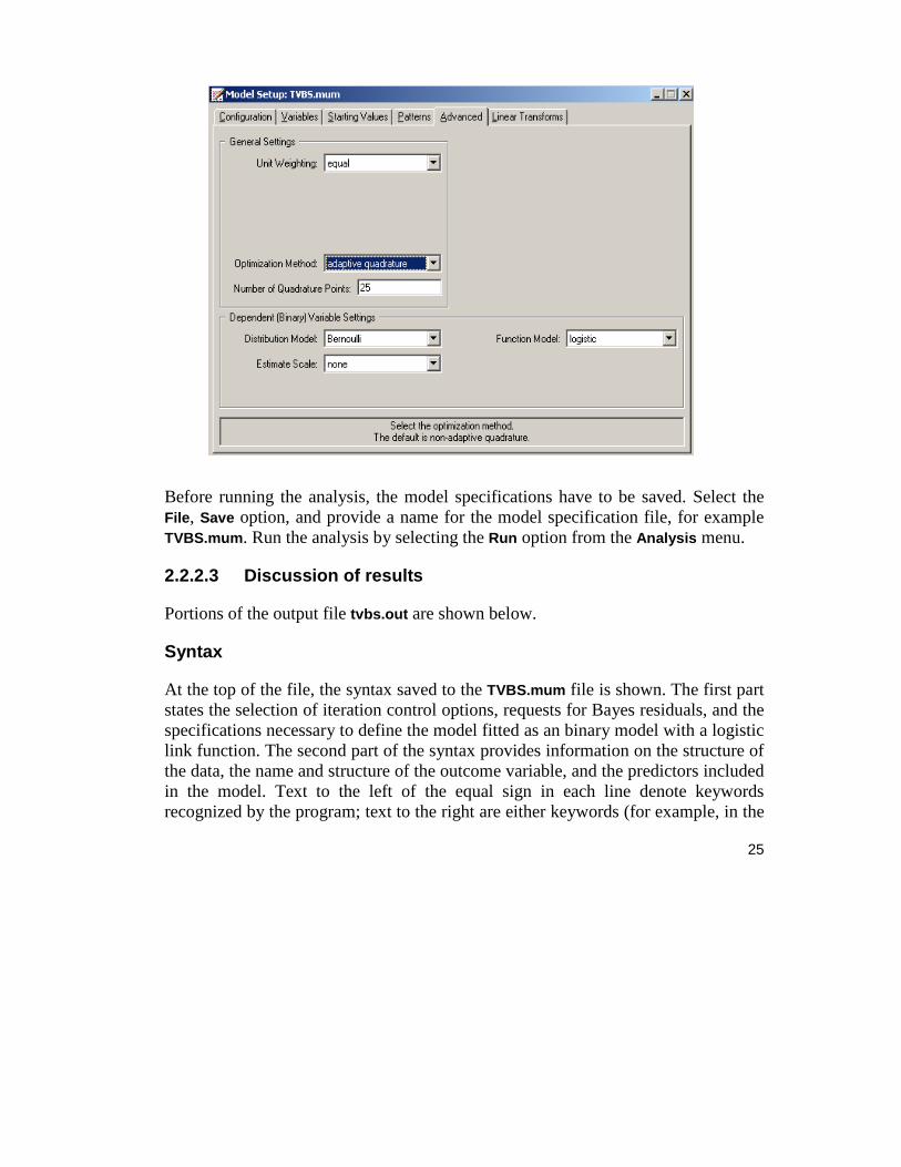
Table XXX.6: Estimated population-average probabilities

Group prescore prob. prescore prob.

CC = 0, TV = 0 0 22.99% 2.152 40.40% CC = 1, TV = 0 0 46.59% 2.05 65.57% CC = 0, TV = 1 0 30.14% 2.87 48.87% CC = 1, TV = 1 0 42.13% 1.979 60.74%

A comparison of these probabilities with the observed ratios given in Table XXX.7 for the control group at the end of the study indicates that the population-average results are slightly closer to the observed ratios than is the case for the unit-specific

results. Recall that 1.0161ijd . The extent of differences between unit-specific

and population-average results is highly dependent on the "scaling" induced by

dividing the sij by ijd .

38

Table XXX.7: Observed and predicted proportions of high post–intervention scores

Group Proportion observed Unit-specific predicted prob.

Population-average predicted prob.

CC = 0, TV = 0 41.57% 40.25% 40.40% CC = 1, TV = 0 63.16% 65.81% 65.57% CC = 0, TV = 1 48.32% 48.85% 48.87% CC = 1, TV = 1 60.31% 60.91% 60.74%

2.2.2.5 Interpreting the contents of the level-2 residual file

In addition to the standard output file, the Write Bayes Estimates field on the Configuration tab of the Model Setup dialog was used to request Bayes estimates for the individual random terms. These estimates are written to the file TVBS.ba2. The first few lines of this file are shown below.

Four pieces of information per school are given:

o all 1s for the level-2 model,

o the school’s ID,

o the value of random intercept,

o the empirical Bayes estimate,

o the associated posterior variance for the school estimate, and

o the name of the associated random coefficient.

39

The mean of the empirical Bayes estimates is – 0.0002. The estimates ranged from – 0.473258 for school 506 to 0.410744 for school 407. In both cases a mass-media intervention procedure was applied, and thus TV = 1, but CC = CC*TV = 0. For students with a PreTHKS score of 3 from each of these schools, this implies

0.473258 0.3741 0.3871(3)

0.473258 0.3741 0.3871(3)

1.062142

1.062142

Prob(THKSbin 1| CC 0,PreTHKS 3, ID 506)1

0.74311

ij

e

e

e

e

40

and

0.410744 0.3741 0.3871(3)

0.410744 0.3741 0.3871(3)

1.946144

1.946144

Prob(THKSbin 1| CC 0,PreTHKS 3, ID 407)1

0.87501

ij

e

e

e

e

respectively. The fact that the intercept for school 407 lies higher than the average is reflected in the higher probability (87.5%) that a student with average pre-intervention knowledge score will obtain a high post-intervention score. School 506, on the other hand, has an intercept far below the average, and a student from this school has, in effect, a 74.31% chance of obtaining a high post-intervention score.

2.2.3 A 2-level random intercept logistic regression model

Using the same data (tvsfpors.ss3) and syntax file TVBS.mum from the previous example, we now consider the situation where students are nested within classrooms and fit a two-level model of the form described earlier, again with the binary variable THKSbin as outcome.

2.2.3.1 Setting up the analysis

Use the File, Open Spreadsheet option to re-open the previously used spreadsheet tvsfpors.ss3 from the Examples\Binary folder. Next, use the File, Open Existing Model Setup option to browse and open the syntax file TVBS.mum.

The biggest change to be made to the syntax file is in terms of the ID variable. Change the Level-2 IDs field on the Configuration tab of the Model Setup dialog box from School to Class, as shown below. Also, turn of the writing out of Bayes estimates by setting the Write Bayes Estimates field to no.

41

Save the revised syntax file under a new name such as TVBC.mum and run the analysis.

2.2.3.2 Discussion of results

Partial output for this run is provided below. The summary of units now reflects the number of students nested within each classroom. The number of students per class (level-2 unit) ranges between 2 and 28. In this analysis, there were 135 level-2 units, compared to 28 in the previous analysis.

42

Estimated coefficients with adaptive quadrature and the estimated level-2 variances are given below.

The estimates for the classroom analysis are very similar to those of the school analysis. All estimated fixed coefficients are slightly lower than was the case in the previous analysis. There seems to be more variation between classrooms than

43

between schools, as indicated by the estimated variation in the random intercept of 0.2193, compared to the similar estimate of 0.1065 in the school analysis.

The estimates can again be used to obtain predicted probabilities by first calculating

the *sij , using the formulae

1.2535 0.9883 CC 0.2870 TV 0.369 CC TV

0.401 PreTHKS

ij i i i

ij

and */ij ij ijd where

2 2

2 2

0.2193 / 3

/ 3

0.2193 3.2898651.0666.

3.289865

ijy

ijd

A comparison of unit-specific and population-average predicted probabilities for the current model are given in Table XXX.8. For comparison purposes, similar results for the previous model can be found in Table XXX.7.

Table XXX.8: Observed and predicted proportions of high post–intervention scores

Group Proportion observed Unit-specific predicted prob.

Population-average predicted prob.

CC = 0, TV = 0 41.57% 40.36% 40.66% CC = 1, TV = 0 63.16% 63.57% 63.16% CC = 0, TV = 1 48.32% 46.76% 46.87% CC = 1, TV = 1 60.31% 60.98% 60.64%

44

2.2.4 A 3-level random intercept logistic regression model

Having fitted 2-level models where students were nested within either classrooms or schools thus far, we now consider a 3-level model with both classroom and school defining levels of the hierarchy.

2.2.4.1 The model

The level-1 and level-2 models are the same as for the previous two models, as shown below.

Level 1 model ( 1 )ijk n :

0 1THKSbin PRETHKSijk ij ij ijk ijkb b

Level-2 model ( 1 )ij n :

0 00 01 02 03 0

1 10

CC TV (CC TV )ij i i ij i ij i ij ij ij

ij i

b b b b b v

b b

With classrooms nested within schools, however, a third level of the hierarchy is defined. At this level, the level-2 coefficients become outcomes again, and can potentially vary over the schools (level-3 units). In the current model, we allow only the intercept to vary randomly over the schools.

Level-3 model ( 1 )i N

00 0 0

01 1

02 2

03 3

10 4

i i

i

i

i

i

b v

b

b

b

b

45

2.2.4.2 Setting up the analysis

We modify our model setup saved to the syntax file TVBS.mum by first using the Open Existing Model Setup option on the File menu to retrieve the syntax file. Then click on File, Save as to save the model setup in a new file, such as TVBSC.mum. Next, select CLASS as the Level-2 ID and SCHOOL as the Level-3 IDs as shown below. We now have both level-2 and level-3 IDs selected.

Keep all the other settings unchanged. Save the changes to the file TVBCS.mum and select the Run option on the Analysis menu to run the analysis.

2.2.4.3 Discussion of results

The portions of the output file TBVSC.out containing the estimates of the fixed and random coefficients in the current model are shown below.

46

Results for this model are compared to those obtained using the two 2-level models in Table XXX.9. Generally, there is close agreement between the models in terms of

47

both the sign and size of the effects. Note that the only intervention method that consistently has an estimated coefficient significantly different from zero is CC. While use of the media intervention (TV) can positively influence the post-intervention score, it seems clear that using both methods simultaneously does not have any real benefits.

Table XXX.9: Comparison of results for three models with binary variable THKSbin as outcome

2-level: 2-level: Coefficient

CLASS as ID SCHOOL as ID 3-level

Fixed effects: estimate -1.2535 -1.228 -1.2465

Intercept standard error 0.1695 0.1949 0.1957 estimate 0.401 0.3871 0.3954

PRETHKS standard error 0.0461 0.0451 0.0463 estimate 0.9883 1.0893 1.0383

CC standard error 0.1973 0.2454 0.2448 estimate 0.287* 0.3741* 0.3325*

TV standard error 0.192 0.235 0.2358 estimate -0.369* -0.5578* -0.4644*

CCxTV standard error 0.2774 0.3403 0.3427 Random effects:

estimate 0.2193 0.1649 Var(between classrooms) standard error 0.0802 0.0813

estimate 0.1065 0.063* Var(between schools) standard error 0.0578 0.0616

*: Not significant at 5% level of significance.

48

2.2.4.4 Interpreting the adaptive quadrature results

3-level ICCs

Intraclass correlation coefficients can be obtained for the three-level dichotomous outcome model. As mentioned earlier, it is assumed that the level-1 error variance is equal to 2 / 3 for the logistic link function if the model is true (see, e.g., Hedeker & Gibbons (2006), p. 157). Using this approximation, the formulae for the standard ICCs can be adjusted.

From the output for the random effects, we have

2Level-1: error var = /3=3.2899

Level-2: class var = 0.1649

Level-3: school var = 0.0630.

Based on this information, we can calculate the ICCs as shown below.

Similarity of students within the same school:

2(3)

2 2 2(3) (2)

0 063

0 063 0.1649 3.28986

0 0179.

v

v v

ICC

49

Similarity of students within the same classrooms (and schools):

2(2)

2 2 2(3) (2)

0 1649

0 063 0.1649 3.28986

0 04688.

v

v v

ICC

Similarity of classes within the same school:

2(2)

2 2(3) (2)

0 1649

0 063 0.1649

0 7236.

v

v v

ICC

Estimated unit-specific and population-average probabilities

Under the assumption that iv , ijv and ijk are independently distributed, it follows

that for the three-level model the design effect is defined as

2 2 2

(3) (2)

2

( )1.0692.v v

ijkd

50

The estimated unit-specific probabilities are calculated using

1.2465 1.0383 CC 0.3325 TV 0.4.644 CC TV

0.3954 PreTHKSijk i i i i

ijk

and

1Prob(THKSbin 1| )

1 ijke

â

The estimated population-average probabilities (Hedeker & Gibbons, 2006) are

obtained in a similar fashion as the unit-specific probabilities after replacing ijk

with */ijk ijk ijkd in the second of the equations shown above.

51

2.3 Models based on the subset of NESARC data

2.3.1 The data

The data set is from the National Epidemiologic Survey on Alcohol and Related Conditions (NESARC), which was designed to be a longitudinal survey with its first wave fielded in 2001-2002. This data file has been used in some of the examples in Chapter XXX. Detailed information about the survey is available at http://niaaa.census.gov/index.html.

In Section 4 of the description of the NESARC study, information on the data regarding occurrences of major depression, family history of major depression and dysthymia are collected. This information was used, in combination with the demographic information provided in Section 1 of the study description, to produce the nesarc_berc.ss3 data set used in this section. The image below shows the first ten records of this data set. There are 2339 dysthymia respondents in the survey; after listwise deletion, the sample size is 1981.

52

The variables of interest are:

o PSU denotes the Census 2000/2001 Supplementary Survey (C2SS) primary sampling unit.

o FINWT represents the NESARC weights sample results used to form national level estimates. The final weight is the product of the NESARC base weight and other individual weighting factors.

o AGE represents the age of the respondent.

o SEX is the gender of the respondent (1 for male, 0 for female).

o FULLTIME is recoded from question S1Q7A1. It is the response to the statement "present situation includes working full time (35+ hours a week)" with 1 indicating yes and 0 indicating no.

o YR2_DEP is the observed response to the statement that the respondent had a period of at least 2 years with low mood, and being sad or depressed most of day (1 = yes, 0 = no.) It is recoded from S4CQ1 in the source data.

o WHITEOTH represents the origin of white and other ethnicities, excluding Black and Hispanic. It is recoded from items S1Q1C, S1Q1D2, S1Q1D3 and S1Q1D5 in the NESARC source code (1 for white and other, 0 for black and Hispanic).

o BLACK represents African American respondents in the sample. It is recoded from S1Q1C and S1Q1D3 (1 for African American, 0 for others).

o HISPANIC is an indicator for Hispanic respondents in the sample data. It is recoded from S1Q1C, S1Q1D3 and S1Q1D5 (1 for Hispanic, 0 for others).

o YOUNG is recoded from AGE. Respondents younger than 35 have the value 1; otherwise, YOUNG = 0.

o MIDDLE is recoded from AGE. Respondents with 35 AGE<50 have the value 1. Otherwise, MIDDLE = 0.

o OLD is recoded from AGE. Respondents with AGE 50 have the value 1. Otherwise, OLD = 0.

53

We recoded the ethnicity variables because of the unbalanced numbers of respondents from different ethnicities in the original NESARC data. While weights are supplied with the data and should be used to adjust for the disproportionality of the sample, the use of indicator variables offers the opportunity to obtain estimated coefficients for individual groups while using one of the other ethnic groups as a reference group. The recoding of ethnicity is discussed in detail in Section XXXXX . Similarly, an explanation of the motivation for the replacement of AGE with 3 indicator variables representing different age groups is given in Section XXXXX.

In this section, we discuss the fitting of three Bernoulli models to these data.

2.3.2 A 2-level random intercept probit model

2.3.2.1 The model

In the previous models (see Section 2.2) the logistic link function was used. We now fit a model by using the probit link function.

The outcome variable of interest is YR2_DEP has the values 0 or 1. For this binary outcome variable

1Prob(YR2_DEP 1| )ij i ij â

where ij represents the log of the odds of success, and can be expressed as

0 1 2 3 0 0AGE SEX FULLTIMEij ij ij ij i i ijb b b b b v e

for the intended model. This transformation, commonly referred to as the probit link function, constrains Prob( 1| )ijy â to lie in the interval (0,1).

54

2.3.2.2 Setting up the analysis

Open the SuperMix spreadsheet nesarc_berc.ss3. From the main menu bar, select the File, New Model Setup option.

o The Configuration screen is the first tab on the Model Setup dialog box. It is used to define the outcome variable and level-2 and level-3 IDs. Some other settings such as missing values, convergence criterion, number of iterations, etc. can also be specified here. For all the available settings, please refer to Chapter XXXX.

To obtain the model shown above, proceed as follows.

o Select the binary option from the Dependent Variable Type drop-down list.

o Select the outcome variable YR2_DEP from the Dependent Variable type drop-down list box.

55

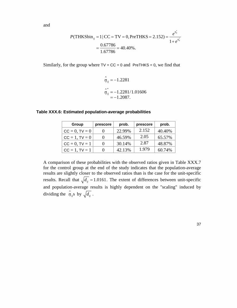
o Select PSU from the Level-2 ID drop-down list box.

o Enter a title for the analysis in the Title text boxes if needed (optional).

o Request a crosstabulation of the outcome variable against AGE by selecting Yes from the Perform Crosstabulation drop-down list box, and select AGE as Crosstab Variable.

o Keep all the other settings on the Configuration screen at their default values. Proceed to the Variables screen by clicking on this tab.

The Variables screen is used to specify the fixed and random effects to be included in the model. Select the explanatory (fixed) variables using the E check boxes next to the variables AGE, SEX and FULLTIME in the Available grid at the left of the screen. After selecting all the explanatory variables, the screen shown below is obtained. The Include Intercept check box in the Explanatory Variables grid is checked by default, indicating that an intercept term will automatically be included in the fixed part of the model.

56

The Advanced tab enables the user to define the weight variable. Weights are often used in complex sampling to adjust the existing sample for known biases. In SuperMix, the weight is normalized by default. To include a weight variable, proceed as follows.

o Select differential from the Unit Weight drop-down list to activate the Assigned Weight.

o Select FINWT from the drop-down list of the Level-1 Weight field.

o Select adaptive quadrature as method of estimation in the Optimization Method field.

Save the model specifications to the file nesarc_ber1.mum and run the analysis.

2.3.2.3 Discussion of results

Portions of the output file nesarc_ber1.out are shown below.

57

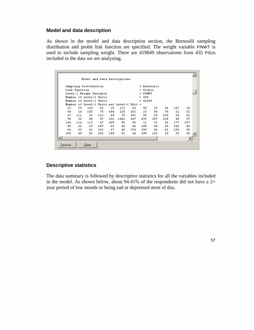
Model and data description

As shown in the model and data description section, the Bernoulli sampling distribution and probit link function are specified. The weight variable FINWT is used to include sampling weight. There are 419849 observations from 435 PSUs included in the data we are analyzing.

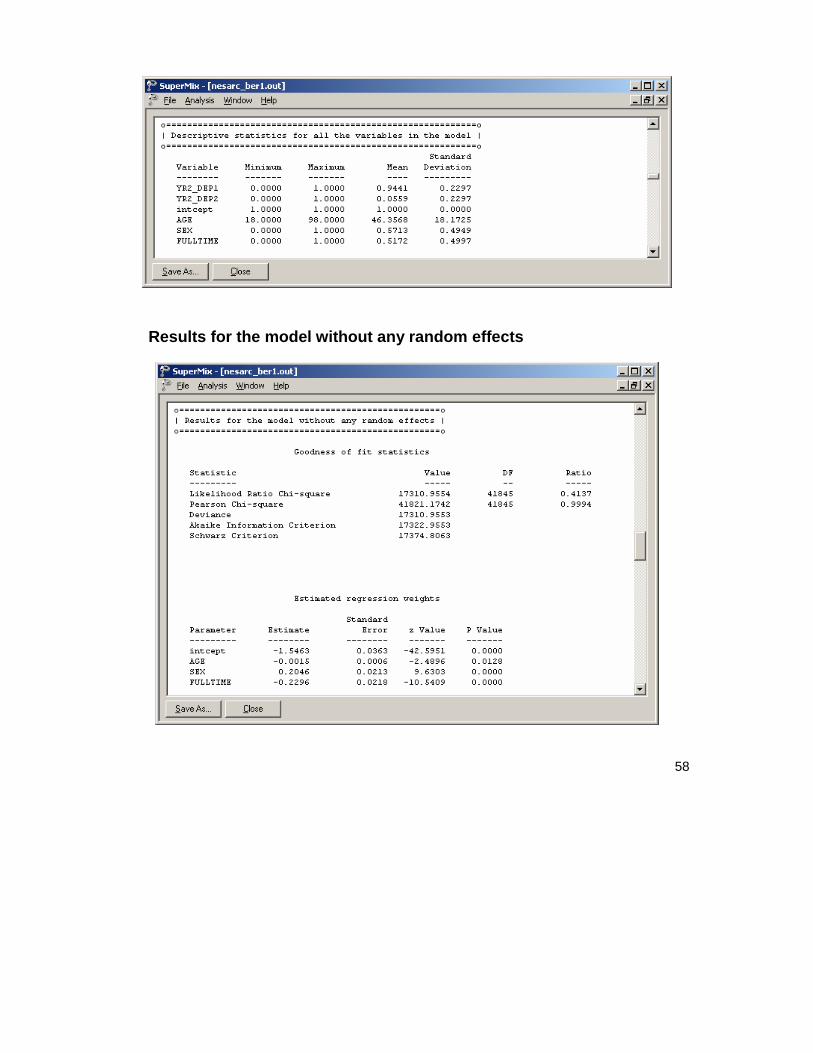
Descriptive statistics

The data summary is followed by descriptive statistics for all the variables included in the model. As shown below, about 94.41% of the respondents did not have a 2+ year period of low moods or being sad or depressed most of day.

58

Results for the model without any random effects

59

Descriptive statistics are followed by the results for the model without any random effects. These results are used as the starting values for the model with random effects.

Results for the model with random effects

The total number of iterations, the goodness of fit statistics and the estimated regression weights are shown below.

The estimated intercept coefficient is -1.5546. The estimated coefficient associated with AGE is – 0.0015, which implies that for every year increase in age of a typical respondent, the estimated probit ˆij is expected to decrease by 0.0015. The

coefficient seems small, but keep in mind that age has a wide range, and

60

consequently this estimate may have a big effect on the overall probability. The estimated coefficient associated with gender is 0.2121, which indicates that the male respondents (SEX = 1) have a larger ˆij . The estimate for the indicator of FULLTIME

shows that respondents with full-time jobs were expected to have a lower ˆij value

than respondents with a similar profile in terms of age and gender but without full-time employment.

2.3.2.4 Interpreting the adaptive quadrature results

The probit link function is now used to transform these estimates into probabilities. First, we substitute the regression weights and obtain an expression for ˆij :

0 1 2 3ˆ ˆ ˆ ˆˆ AGE SEX FULLTIME

1.5546 0.0015 AGE 0.2121 SEX 0.23 FULLTIME .

ij i i i iij ij ij

ij ij ij

b b b b

For a typical 30-year-old male with a full-time job, SEX = 1, FULLTIME = 1 and AGE = 30, and thus

ˆ 1.5546 0.0015 30 0.2121 0.23

1.6025.ij

.

Transform the ˆij into the corresponding probability by using the probit link

function:

1Prob(YR2_DEP 1) 1.60937 0.0545.ij

In terms of percentages, 5.45% of males with this profile would be expected to suffer from long-term depression episodes. Similarly, the probability of having a depression episode of 2+ years’ duration for different gender and age combinations can be calculated. These probabilities, expressed as percentages, are reported in Table XXX.10 below.

61

Table XXX.10: % probabilities of having a depression episode

Age 20 30 40 50 60 70

not fulltime, female 5.65% 5.48% 5.32% 5.16% 5.00% 4.85% not fulltime, male 8.50% 8.26% 8.04% 7.82% 7.60% 7.39% fulltime, female 3.48% 3.37% 3.25% 3.15% 3.04% 2.94% fulltime, male 5.45% 5.29% 5.13% 4.97% 4.82% 4.67%

In general, males without full-time employment were more likely to have depression episodes than their female counterparts. Surprisingly, this is also true of males with full-time employment.

These probabilities can also be depicted in a line plot as shown below. The line associated with males without full-time jobs is considerably higher than for any other groups, again illustrating that this group has the highest probability of having 2+ years’ period with low mood regardless of their age. For all the correspondents, as they grow older, the probability of having lengthy depression episodes decreased.

Figure XXX.5: Expected probabilities for subgroups

62

2.3.3 A 2-level random intercept model with additional predictors

2.3.3.1 The model

In the previous section, we modeled the outcome variable YR2_DEP in terms of its relationship with the predictors AGE, SEX and FULLTIME. The model discussed in this section takes the ethnicity of patients into consideration by including two dummy variables, BLACK and HISP. Since the group of WHITEOTH is not included, it is automatically regarded as the reference category.

For the current model, the log of the odds of success ( ij ) can be expressed as

0 1 2 3 4 5

0

AGE SEX FULLTIME BLACK HISP

.ij ij ij ij ij ij

i ij

b b b b b b

v e

2.3.3.2 Setting up the analysis

We can modify the model setup file nesarc_ber1.ss3 by opening it and then saving it under a different name, such as nesarc_ber2.ss3.

Click on the Variables tab of the Model Setup window. Add the predictors BLACK and HISP to the model by checking the boxes next to these variables in the E column, as shown below.

63

Save the modified model specification file, and select the Run option from the Analysis menu to perform the analysis.

2.3.3.3 Discussion of results

Portions of the output file nesarc_berc2.out are shown below.

Results for the model fitted with adaptive quadrature

The goodness of fit statistics are shown below. Since the previous model can be considered as a submodel of the current model, the deviances of these two models can be used to perform a 2 test to evaluate possible improvement in model fit.

64

The output describing the estimated fixed effects after convergence is shown next. As shown above the estimated logit for the intercept is -1.5071, the estimated logit associated with AGE is -0.002, etc. It is interesting to note that the only positive estimate is for gender. Males are thus more likely to show long-term depression, while it will be less likely in those who are older or fully employed. The ethnicity indicators' coefficients also indicate that white respondents are most likely to have depression, with the Hispanic population the least likely.

65

2.3.3.4 Interpreting the adaptive quadrature results

Estimated outcomes for different groups: unit-specific results

To evaluate the simultaneous impact of these estimates on the expected probabilities for respondents from the subgroups formed by the categories of age, gender, and ethnicity, we may use the estimated regression weights and the link function to calculate probabilities of having depression in the same way as for the previous model.

For the current model, ij can be expressed as:

1.5071 0.0020 AGE 0.2121 SEX 0.2335 FULLTIME

0.0891 BLACK 0.1816 HISP .

ij ij ij ij

ij ij

Table XXX.11 contains a subset of these estimated probabilities. Only typical respondents 30 or 50 years old are considered here, and probabilities are expressed as percentages.

Table XXX.11: % Probabilities of having depression episodes for selected age groups

Age 30 50

Ethnicity White Black Hispanic White Black Hispanic

not fulltime, female 5.85% 4.88% 4.02% 5.40% 4.49% 3.68% not fulltime, male 8.77% 7.44% 6.22% 8.15% 6.89% 5.74% fulltime, female 3.59% 2.94% 2.37% 3.28% 2.68% 2.16% fulltime, male 5.61% 4.67% 3.84% 5.17% 4.29% 3.51%

66

Younger white males without full-time employment have the highest risk of having long-term depression, while female Hispanic respondents with full-time employment were least at risk.

The results in Table XXX.11 can also be depicted as a bar chart. Figure xxx.6 shows that white respondents are more likely to get depressed for a long period than African American or Hispanic respondents.

Figure XXX.6: Estimated probabilities for subgroups

Model comparison

Since the two models in this section are nested models, the chi-square difference test can be used. The deviances, AIC, and SBC statistics for these models are summarized in Table XXX.12. These statistics suggest that the second model fits the data better.

Table XXX12: Model comparison

Statistic Model 1 Model 2 difference Difference

in d.f.

2ln L (deviance statistic) 17203.107 17176.699 26.4078 2 Akaike Information Criterion 17213.107 17190.699 22.4078 2 Schwarz Criterion 17256.316 17251.192 5.12415 2

67

References

Krommer, A.R. & Ueberhuber, C.W. (1994). Numerical Integration on advanced computer systems. New York: Springer-Verlag.

Stroud, A.H. & Secrest, D. (1966). Gaussian quadrature formulas. New Jersey: Prentice-Hall.

McCullagh & Nelder, 1989

Flay, et. al., 1988

Hedeker & Gibbons, 2006

National Epidemiologic Survey on Alcohol and Related Conditions (NESARC)