· 2 CHAPTER 1. INTRODUCTION Document structure...

Université Libre de Bruxelles

The TESLA coil Christopher Gerekos,

2nd year Physics undergraduate student.

“Let the future tell the truth and evaluate each one according to his work and accomplishments.

The present is theirs; the future, for which I really worked, is mine.”

-Nikola Tesla

2011-2012

Special thanks

This Tesla coil never would have existed without my friend Mael Flament, former student at the UniversitéLibre de Bruxelles, now studying at the Hawaii University (Manoa). He initiated the idea of this projectand taught me the basics of electrical engineering and crafting.

I also thank Kevin Wilson, creator of the TeslaMap program and webmaster of Tesla Coil Design,Construction and Operation Guide i, which were my main guides during the early stages of the conceptionand construction of the coil. He also proofread this English version of the present document.

Thanks to Thomas Vandermergel for his participation in the Printemps des Sciences fair and to Jean-Louis Colot for his guidance and his awesome photographs of Zeus.

I also express my full gratitude to my family for their support.

iReferenced in the Bibliography.

Contents

1 Introduction 1

2 The Zeus Project 3

3 Theory of operation 53.1 Reminder of the basics . . . . . . . . . . . . . . . . . . . . . . . . . . . . . . . . . . . . . . . 5

3.1.1 Resistor . . . . . . . . . . . . . . . . . . . . . . . . . . . . . . . . . . . . . . . . . . . 53.1.2 Capacitor . . . . . . . . . . . . . . . . . . . . . . . . . . . . . . . . . . . . . . . . . . 63.1.3 Inductor . . . . . . . . . . . . . . . . . . . . . . . . . . . . . . . . . . . . . . . . . . . 63.1.4 Impedance . . . . . . . . . . . . . . . . . . . . . . . . . . . . . . . . . . . . . . . . . 7

3.2 LC circuit . . . . . . . . . . . . . . . . . . . . . . . . . . . . . . . . . . . . . . . . . . . . . . 83.2.1 Impedance . . . . . . . . . . . . . . . . . . . . . . . . . . . . . . . . . . . . . . . . . 123.2.2 Resonant frequency . . . . . . . . . . . . . . . . . . . . . . . . . . . . . . . . . . . . 133.2.3 RLC circuit . . . . . . . . . . . . . . . . . . . . . . . . . . . . . . . . . . . . . . . . . 13

3.3 Tesla coil operation . . . . . . . . . . . . . . . . . . . . . . . . . . . . . . . . . . . . . . . . . 153.3.1 Description of a cycle . . . . . . . . . . . . . . . . . . . . . . . . . . . . . . . . . . . 153.3.2 Voltage gain . . . . . . . . . . . . . . . . . . . . . . . . . . . . . . . . . . . . . . . . . 193.3.3 Comparison with the induction transformer . . . . . . . . . . . . . . . . . . . . . . . 203.3.4 Distribution of capacitance within the secondary circuit . . . . . . . . . . . . . . . . 213.3.5 Influence of the coupling . . . . . . . . . . . . . . . . . . . . . . . . . . . . . . . . . . 223.3.6 A few words on the three-coil transmitter . . . . . . . . . . . . . . . . . . . . . . . . 23

3.4 The quarter-wave antenna . . . . . . . . . . . . . . . . . . . . . . . . . . . . . . . . . . . . . 243.4.1 Comparison with the Tesla coil . . . . . . . . . . . . . . . . . . . . . . . . . . . . . . 24

4 Conception and construction 264.1 HV transformer . . . . . . . . . . . . . . . . . . . . . . . . . . . . . . . . . . . . . . . . . . . 26

4.1.1 Arc length . . . . . . . . . . . . . . . . . . . . . . . . . . . . . . . . . . . . . . . . . . 284.2 Primary circuit . . . . . . . . . . . . . . . . . . . . . . . . . . . . . . . . . . . . . . . . . . . 29

4.2.1 Capacitor . . . . . . . . . . . . . . . . . . . . . . . . . . . . . . . . . . . . . . . . . . 294.2.2 Charge at resonance . . . . . . . . . . . . . . . . . . . . . . . . . . . . . . . . . . . . 364.2.3 Inductance . . . . . . . . . . . . . . . . . . . . . . . . . . . . . . . . . . . . . . . . . 38

4.3 Spark gap . . . . . . . . . . . . . . . . . . . . . . . . . . . . . . . . . . . . . . . . . . . . . . 424.4 Secondary circuit . . . . . . . . . . . . . . . . . . . . . . . . . . . . . . . . . . . . . . . . . . 45

4.4.1 Coil . . . . . . . . . . . . . . . . . . . . . . . . . . . . . . . . . . . . . . . . . . . . . 454.4.2 Top load . . . . . . . . . . . . . . . . . . . . . . . . . . . . . . . . . . . . . . . . . . . 48

4.5 Resonance tuning . . . . . . . . . . . . . . . . . . . . . . . . . . . . . . . . . . . . . . . . . . 514.6 RF ground . . . . . . . . . . . . . . . . . . . . . . . . . . . . . . . . . . . . . . . . . . . . . 524.7 Other components . . . . . . . . . . . . . . . . . . . . . . . . . . . . . . . . . . . . . . . . . 53

vi CONTENTS

4.7.1 NST protection filter . . . . . . . . . . . . . . . . . . . . . . . . . . . . . . . . . . . . 534.7.2 PFC capacitor . . . . . . . . . . . . . . . . . . . . . . . . . . . . . . . . . . . . . . . 544.7.3 AC line filter . . . . . . . . . . . . . . . . . . . . . . . . . . . . . . . . . . . . . . . . 56

4.8 Last step . . . . . . . . . . . . . . . . . . . . . . . . . . . . . . . . . . . . . . . . . . . . . . 56

5 Nikola Tesla, a mind ahead of its time. 57

Appendices 59

A Specifications of the Zeus Tesla coil 60

B Behavior of the signal in the secondary coil 63

C Analysis of the RLC circuit 65

D Analysis of two inductively coupled oscillating circuits. 67D.1 Two coupled LC circuits . . . . . . . . . . . . . . . . . . . . . . . . . . . . . . . . . . . . . . 67D.2 Two coupled RLC circuits . . . . . . . . . . . . . . . . . . . . . . . . . . . . . . . . . . . . . 70

References 75

Bibliography 76

Chapter 1

Introduction

The device we now call a "Tesla coil" is probably the most famous invention of Nikola Tesla. On the patenthe submitted in 1914 to the US Patent & Trademark Office, it was called "Appartus for transmittingelectrical energy" i

Nikola Tesla was born the 10th of July 1856 in a Serbian village of the Austrian Empire (in today’sCroatia) and died the 7th of January 1943 in the United States [1].

It is not an exaggeration to say he was a visionary who changed the world. With his works onalternative current, including many patents on generators, transformers and turbines, he allowed thewidespread proliferation of electricity as a source of power as we know it today.

He was also a pioneer in the domain of telecommunications ; the Tesla coil can be viewed as one ofthe very first attempts of a radio antenna. It consisted of circuits that are fundamentally the same as ourmodern wireless devices.

Figure 1.1: Nikola Tesla in 1890.Figure 1.2: His first laboratory in Colorado Springs.[Photographs : Wikimedia Commons]

iThe front picture is a drawing associated with this patent. See Bibliography.

1

2 CHAPTER 1. INTRODUCTION

Document structureThis document is about the theory of operation of Tesla coils as well as the specific behavior of its individualcomponents. It also relates the steps of the construction of my own first coil, Zeus.

We will only discuss the conventional Tesla coil, consisting of a spark gap and two tank circuits andcalled Spark Gap Tesla Coil (SGTC). In fact, Nikola Tesla also conceived a more advanced type of coil,the magnifying transmitter, which is made of three coils instead of two and which operates in a slightlymore complicated manor. In addition, there is also a class of semiconductors-controlled Tesla coils calledSolid State Tesla Coils (SSTC), which are structurally different but share the same theoretical basis of theconventional Tesla coil.

To fully appreciate this document, it is recommended that you master the fundamental concepts ofelectromagnetism and alternating currentii, as well as the basics of differential equations.

iiAll About Circuits (http://www.allaboutcircuits.com) is an excellent on-line resource. Volumes I and II largely spanthe "engineering" part of the aforementioned perquisites.

http://www.allaboutcircuits.com

Chapter 2

The Zeus Project

This Tesla coil was presented to the Printemps des Sciences 2012 science fair and is now at the Expéri-mentarium de Physique science museum at ULB. It was named Zeus (Ζεύς in ancient Greek or Δίας inmodern Greek) ; in honor of the Greek god, king of the Olympians and known for throwing lightning bolts.

It has a power of 225 W, which is quite low compared to the coils built by professionals, which oftensurpass several thousands of Watts. It is nevertheless an appreciable power, given the small budget thatwas allocated.

Figure 2.1: The Zeus Coil.

The construction of Zeus was not an easy task and almost every component had to be rebuilt at leasttwice. This however allowed me to acquire my first experience in the domain of high voltages, which wasprobably the greatest reward this project gave me.

3

4 CHAPTER 2. THE ZEUS PROJECT

Figure 2.2: Cool beautiful arcs. 1s shutter speed [Photographs: Jean-Louis Colot].

Chapter 3

Theory of operation

In this chapter, we will discuss the theory of operation of Tesla coils in a general way. For the moment,let us introduce this short definition:

A Tesla coil is a device producing a high frequency current, at a very high voltage but of relatively smallintensity.

Basically, it works as a transformer and as a radio antenna, even if it differs radically from these.

Figure 3.1: Basic electric schematic of a Tesla coil. [Schematic : Wikipedia]

3.1 Reminder of the basics

3.1.1 Resistor

Figure 3.2: Symbol ofa resistor.

A resistor is a component that opposes a flowing current.Every conductor has a certain resistancei If one applies a potential difference

V at the terminals of a resistor, the current I passing through it is given by

I =V

R(3.1)

This formula is know as Ohm’s Law ii. The SI unit of resistance is the Ohm, [Ω].

iExcept supraconductors, which have a strictly zero resistance.iiGeorg Simon Ohm : German physicist, 1789-1854.

5

6 CHAPTER 3. THEORY OF OPERATION

One can show that the power P (in J/s) dissipated due to a resistance is equal to

P = V I = RI2 (3.2)

3.1.2 Capacitor

Figure 3.3: Symbol ofa capacitor.

A capacitor is a component that can store energy in the form of an electric field.Less abstractly, it is composed in its most basic form of two electrodes separated

by a dielectric medium. If there is a potential difference V between those twoelectrodes, charges will accumulates on those electrodes : a charge Q on the positiveelectrode and an opposite charge −Q on the negative one. An electrical fieldtherefore arise between them. If both of the electrodes carry the same amount ofcharge, one can write

Q = CV (3.3)

where C is the capacity of the capacitor. Its unit is the Farad iii [F].The energy E stored in a capacitor (in Joules) is given by

E =1

2QV =

1

2CV 2 (3.4)

where one can note that the dependence in the charge Q shows that the energy is indeed the energy ofthe electric field. This corresponds to the amount of work that has to be done to place the charges on theelectrodes.

3.1.3 Inductor

Figure 3.4: Symbol ofan inductor

An inductor stores the energy in the form a magnetic field.Every electrical circuit is characterized by a certain inductance. When current

flows within a circuit, it generate a magnetic field B that can be calculated fromMaxwell-Ampere’s lawiv :

∇×B = µ0J + µ0ε0∂E

∂t(3.5)

where E is the electric field and J is the current density. The auto-inductance of a circuit measures itstendency to oppose a change in current : when the current changes, the flux of magnetic field ΦB thatcrosses the circuit changes. That leads to the apparition of an "electromotive force"v E that opposes thischange. It is given by

E = −∂ΦB∂t

(3.6)

The inductance L of a circuit is thus defined as :

V = L∂I

∂t(3.7)

iiiMichael Faraday : British physicist and chemist, 1791-1867.ivJames Clerk Maxwell, Scottish physicist and mathematician, 1831-1879. André-Marie Ampère, French physicist and

mathematician, 1755-1836.vThis is not properly a force, as the units of E are Volts. The point is that we cannot talk of a potential difference between

two points, as the current flows without a material voltage generator.

3.1. REMINDER OF THE BASICS 7

where I(t) is the current that flows in the circuit and V the electromotive force (emf) that a change ofthis current will provoke. The inductance is measured in henrysvi [H].

The energy E (in Joules) stored in an inductor is given by

E =1

2LI2 (3.8)

where the dependence in the current I shows that this energy originates from the magnetic field. Itcorresponds to the work that has to be done against the emf to establish the current in the circuit.

3.1.4 Impedance

The impedance of a component expresses its resistance to an alternating current (i.e. sinusoidal). Thisquantity generalizes the notion of resistance. Indeed, when dealing with alternating current, a componentcan act both on the amplitude and the phase of the signal.

Expressions for alternating current

It is convenient to use the complex plan to represent the impedance. The switching between the two rep-resentations is accomplished by using Euler’s formula. Let’s note that the utilization of complex numbersis a simple mathematical trick, as it is understood that only the real part of these quantities is meaningful.We are now given an expression of the general form of the voltage V(t) and current I(t) :

V (t) = V0 · cos (ωt+ φV ) ⇔ V (t) = V0 · Reej(ωt−φV )

(3.9)

I(t) = I0 · cos (ωt+ φI) ⇔ I(t) = I0 · Reej(ωt−φI)

(3.10)

where V0 and I0 are the respective amplitudes, ω = 2πν is the angular speed (assumed identical for bothquantities) and φ are the phases.

Definition of impedance

The impedance, generally noted Z, is formed of a real part, the resistance R, and an imaginary part, thereactance X :

Z = R+ jX (cartesian form) (3.11)= |Z|ejθ (polar form) (3.12)

where j is the imaginary unit number, i.e. j2 = −1, theta = arctan(X/R) is the phase difference betweenvoltage and current, and |Z| =

√R2 +X2 is the euclidean norm of Z in the complex plane.

At this point, we can generalize Ohm’s law as the following :

V (t) = Z · I(t) (3.13)

When the component only acts on the amplitude, in other words when X = 0, the imaginary partvanishes and we find Z = R. We therefore have the behavior of a resistor. The component is then said tobe purely resistive, and the DC version of Ohm’s law (3.1) applies.

When the component only acts on the phase of the signal, that is when R = 0, the impedance is purelyimaginary. This translates the behavior of "perfect" capacitors and inductors.

viJoseph Herny, American physicist, 1797-1878.


Figure 3.5: The impedance Z plotted in the complex plane. [Diagram : Wikipedia]

Impedance formulas

We can give a general formula for the impedance of each type of component.

Component Impedance Effect on an alternating signal

Resistor Z = R Diminution of amplitude (current and tension).

Capacitor Z = 1jCω Tension has a π/2 delay over current.

Inductor Z = jLω Current has a π/2 delay over tension.

These formulas are easily recovered from the differential expressions of these components. For everycombinations of components, one can calculate the phase difference between current and voltage by vector-adding the impedances (for example, in an RC circuit, the phase difference will be less than π/2).

Finally, it is good to keep in mind that any real-life component has a non-zero resistance and reactance.Even the simplest circuit, a wire connected to a generator has a capacitance, an inductance and a resistance,however small these might be.

3.2 LC circuitAn LC circuit is formed with a capacitor C and an inductor L connected in parallel or in series toa sinusoidal signal generator. The understanding of this circuit is at the very basis of the Tesla coilfunctioning, hence the following analysis.

The primary and secondary circuits of a Tesla coil are both series LC circuitsvii that are magneticallycoupled to a certain degree. We will therefore only look at the case of the series LC circuit.

Figure 3.6: Schematic of a series LC circuit.

Using Kirchoff’s law for current, we obtain that the current in the inductor and the current in thecapacitor is identical. We now use Kirchoff’s law for voltage, which sates that the sum of the voltages

viiOf course, they’re actually RLC circuits, which, we’ll talk about later, as all the components and wires have a certainresistance. However, materials used as well as the section of the conductors keep this resistance negligible. We can thereforeconsider in first approximation that the real circuits behave like LC circuits.

3.2. LC CIRCUIT 9

across the components along a closed loop is zero, to get the following equation :

Vgen(t) = VL(t) + VC(t) (3.14)

For the inductor, we use the equality (3.7) and express the time derivative of current in terms of thecharge by I = dQ

dt . We find

VL(t) = LdI

dt(3.15)

= Ld2Q

dt2(3.16)

Now for the capacitor, we isolate the charge Q in the relation (3.3) and get

VC(t) =1

CQ(t) (3.17)

Plugging these two results in (3.14), we obtain :

Vgen(t) = LQ+1

CQ (3.18)

This equation describes an (undamped) harmonic oscillator with periodic driving, just like a spring-masssystem! The inductor is assimilated to the "mass" of the oscillator : a circuit of great inductance will havea lot of "inertia". The "spring constant" is associated with the inverse of the capacitance C−1 (this is thereason why C−1 is seldom called the "elastance").

Homogeneous solution

The homogeneous equation, i.e. without independent term (representing the generator, in this case) is thefollowing :

LQ+1

CQ = 0 (3.19)

This equation corresponds to a real situation: the capacitor holds a certain charge and we let thesystem evolute freely. The mechanical analogy with the spring-mass system correspond to an initial statewhere the spring is tense and when no other force interactsviii

We find the solution to equation (3.19) with the characteristic polynomial method. We obtain a sumof complex exponentials, which is of course an oscillating solution as expected.

Q(t) = K1ejωt +K2e

−jωt (3.20)

where we noted ω ≡ 1/√LC.

Setting Q(0) ≡ Q0 and Q(0) = I(0) ≡ 0, which indeed corresponds to the initial condition where thecapacitor is fully loaded and no current initially flows in the inductor, we get

K1

2= Q0 =

K2

2(3.21)

We now take the real part of Q(t), but thanks to (3.21), the solution is already real :

Q(t) = Q0 cos (ωt) = Q0 cos

(t√LC

)(3.22)

viiiEquation (3.19) has of course the trivial solution Q(t) = 0 ∀t, but we won’t consider it here.


We now find the current flows through the inductor by time-derivating the above expression for thecharge stored in the capacitor :

I(t) = − Q0√LC

sin

(t√LC

)(3.23)

The next figures give a good intuition of what actually happens in the circuit. We look at the voltageV (t) between the leads of the capacitor as well as the current I(t) running into the inductor (which is thesame in the entire circuit, as previously stated). For convenience, we put all the constants Q0, L, and Cto unity.

Figure 3.7: LC circuits with voltmeter and ammeter Figure 3.8: Plot of tension in current versus time.

Step 0: At the initial instant, the capacitor is fully charged and no current flows. Immediately after,the capacitor begins to discharge: the voltage decreases as a current gradually appears in the circuit.

Step 1: When the capacitor is totally discharged, the voltages at its leads is zero. If there was noinductance, things would stop right here. However, the inductor opposes this brutal drop of current bygenerating an electromotive force that will keep the current goingix. In this way, the current graduallydecreases (instead of stopping abruptly) and recharges the capacitor on the way (with an opposite polarity).

Step 2: The capacitor is fully charged again, with opposite polarity now, and the current has fallen tozero. However the charges stored in the capacitor are wanting to neutralize themselvesx : a current willreappear while the voltage is decreasing again.

Step 3: The capacitor is "empty" again (zero voltage), but the inductor prevents the current fromstopping abruptly. This current will now recharge the capacitor with reversed polarity ...

Step 4: ... and the situation is exactly like it was at the initial instant.

We have already noted at this point that the system naturally oscillates at a certain resonant angularspeed ω = 1√

LC, which is univoquely determined by the inductance and the capacitance of the circuit.

ixLet us remember the mechanical analogy :inductance gives "inertia" to the circuits.xJust like a tense spring wants to recover its neutral shape.

3.2. LC CIRCUIT 11

General solution.

We reconsider equation (3.18) with its independent term, where we explicitly state the fact that thegenerator produces a sinusoidal voltage of amplitude, say, V0 and of pulsation Ω:

LQ+1

CQ = V0 sin (Ωt) (3.24)

We will find a specific solution to obtain the general solution

If ω 6= Ω. We make an educated guess about a specific solution Qp by stating it has the following form:Qp = A sin (Ωt− ϕ), with amplitude A and phase ϕ to be determined. We derivate this guessed solutiontwice and inject it straight into our starting equation (3.24) :

A

[1

C− Ω2L

]sin (Ωt− ϕ) = V0 sin (Ωt) (3.25)

Equating amplitude and phase into the two parts of this equality, we deduce :A = V0

1/C−Ω2L = V0

L(ω2−Ω2)

ϕ = 0(3.26)

The specific solution is therefore :

Qp(t) =V0

L(ω2 − Ω2)sin (Ωt) (3.27)

We can now find the general solution by adding the specific solution to the homogeneous solution(3.20).

Q(t) = K1 cos (ωt) + K2 sin (ωt) +V0

L(ω2 − Ω2)sin (Ωt) (3.28)

The current is :

I(t) = ωK2 cos (ωt)− ωK1 sin (ωt) +V0Ω

L(ω2 − Ω2)cos (Ωt) (3.29)

where the constants K1 and K2 can be found in terms of the initial conditions.We see that we still have sinusoidal functions. If ω is close to Ω, the oscillations will be of great

amplitude because of the "new" term, but will remain bounded. When ω is very far from Ω, the new termbecomes negligible.

If ω = Ω. Here, the specific solution is more difficult to find. Let us rewrite (3.24) in a more convenientway :

Q+ ω2Q =V0

2Lj(ejωt − e−jωt) (3.30)

Here, we’ll guess that the specific solution has the following form ; Qp(t) = (A+ + B+t)ejωt + (A− +

B−t)e−jωt. This makes sense physically, as we expect the voltage and current to have amplitudes that

increase with time. We rewrite it in a more condensed manner : Qp(t) = (A+Bt)ekt with k = ±jω. Thesecond time-derivative yields Qp(t) =

[k2(A+Bt) + 2kB

]ekt. We plug thses expression in (3.30) in order

to refine them : [(k2 + ω2)(A+Bt) + 2kB

]ekt = ± V0

2Ljekt (3.31)


We compare the two side of the equality as before.When k = jω, we find

2jωB+ejωt =

V0

2Ljejωt (3.32)

B+ =V0

4Lω(3.33)

When k = −jω,

− 2jωB−e−jωt = − V0

2Lje−jωt (3.34)

B− =V0

4Lω(3.35)

We have therefore found that B+ = B− ≡ B. And as we have found no constraints on the A’s, we setthem equal to zero. We have now obtained our specific solution :

Qp(t) = Btejωt +Bte−jωt (3.36)

=V0t

4Lω

(ejωt + e−jωt

)(3.37)

=V0t

2Lωcos (ωt) (3.38)

The general solution for the voltage is therefore :

Q(t) = K1 cos (ωt) + K2 sin (ωt) +V0t

2Lωcos (ωt) (3.39)

and the current is :

I(t) =

(ωK2 −

V0

2Lω

)cos (ωt)− ωK1 sin (ωt)− V0ωt

2Lωsin (ωt) (3.40)

where the constants K1 and K2 can be found in terms of the initial conditions.In this case, we see we’re no longer dealing with simple oscillations. The last term of the solution

indicates that the amplitude of the voltage and current will increase at each cycle, and grow to infinity ast→∞.

3.2.1 ImpedanceWe’ll have to calculate the impedance of the LC circuits inside the Tesla coil. Let us recall that thecapacitor and the inductor are connected in series on the generator. The total impedance is thereforeequal to the sum of the impedances of each component.

Z = ZC + ZL (3.41)

=1

jCω+ jLω (3.42)

= jω2LC − 1

ωC(3.43)

We see that, at the resonant pulsation, ω2LC = 1 and the impedance vanishes. A series LC circuitplaced in series on a wire will therefore act as a band-pass filter. Similarly, a parallel LC circuit will act asa band-stop filter when connected in series on the wire [2]. There are many other possibilities for filters,but this is not within the scope of the present document.

3.2. LC CIRCUIT 13

3.2.2 Resonant frequencyIn our analysis of the LC circuit, we found that the oscillations of current and voltage naturally occurred ata precise angular speed, univoquely determined by the capacitance and inductance of the circuit. Withoutother effects, oscillations of current and voltage will always take place at this angular speed.

ωres =1√LC

(3.44)

It is called the resonant angular speed. We can check that it is dimensionally coherent (its units are s−1).It is however much more common to talk about resonant frequency, which is just a rescale of the angular

speed :

fres =1

2π√LC

(3.45)

It is no less important to observe that, at the resonant angular speed, the respective reactive parts ofan inductor and a capacitor are equal (in absolute value) :

|XresL | =

L√LC

=

√L√C

= |XresC | (3.46)

When there is a sinusoidal signal generator, we also saw that if its frequency is equal to the resonantfrequency of the circuit it drives, current and voltage have ever-increasing amplitudes. Of course, thisdoesn’t happen if they are different (the oscillation remain bounded).

Figure 3.9: Amplitude of the current plotted against the driving frequency (all constants normalized). [Diagram :Wikipedia]

At low driving frequencies, the impedance is mainly capacitive as the reactance of a capacitor is greaterat low frequencies. At high frequencies, the impedance is mainly inductive. At the resonant frequency,it vanishes, hence the asymptotic behavior of the current. However, in a real circuit, where resistance isnon-zero, the width and height of the "spike" plotted her above are determined by the Q factor, whichwe’ll talk about later.

The fact that driving an (R)LC circuit at its resonant frequency causes a dramatic increase of voltageand current is crucial for a Tesla coil. But it can also be potentially harmful for the transformer feedingthe primary circuit. These practical considerations will be addressed in the next chapter.

3.2.3 RLC circuitAn RLC circuit is an LC circuit on which a resistance was added. This kind of circuit can take multipleforms. We won’t analyze it here, but we’ll give its major characteristicsxi.

xiA thorough treatment is given in Appendix C.


Figure 3.10: Schematic of a series RLC circuit.

Figure 3.11: Amplitude of the current vs driving frequencyfor an RLC circuit (all constants normalized). [Diagram: Wikipedia]

The resistance (VR(t) = RQ′(t)) dissipates the circuits energy as heat, whatever the direction of thecurrent. It therefore acts like a friction force. Without a generator, current and voltage will graduallydecrease as they oscillate (the circuit is said to be underdamped) or, if the resistance is high enough, nooscillation will take place (overdamped circuit).

In the underdamped case, the graph of current or voltage is a sine wave whose amplitude decreasesexponentially with time. If there is a driving force, the resistance will prevent the system from havingoscillations of ever-increasing amplitude. And finally, instead of a spike, the RLC circuit has a bandwidth.

One can show that the resonant frequency of a RLC circuit is the same as the LC circuit [3][4]:

fres =1

2π√LC

(3.47)

To find its impedance, we just have to add the value of the resistance R to (3.43). While the LC circuithad a purely imaginary impedance, the RLC circuit has a real part as well :

Z = R+ j

(ωL− 1

ωC

)(3.48)

Q factor.

The Q factor (for quality) is a dimensionless quantity which characterizes every RLC circuit, or moregenerally, every damped oscillator. It measures the narrowness of the bandwidth : a large Q factordenotes a spiky bandwidthxii.

More precisely, the Q factor represents the ratio between the energy stored in the circuit and the energydissipated during the oscillations [5]. This can also be expressed in power terms [6] :

Q =Pstored

Pdissipated=XI2

RI2(3.49)

=X

R(3.50)

where X is the reactance of the inductor/capacitor at the resonant frequency.For a RLC circuit, this becomes, using (3.45) :

Q =1

R

√L

C(3.51)

xiiIn the stricter sense, the Q factor of a LC circuit is infinite, but the quantity is not really meaningful in this case.

3.3. TESLA COIL OPERATION 15

One can also give a definition of the bandwidth ∆f as a function of the Q factor [6] :

∆f =fresQ

(3.52)

It is then clear why this quantity is called the quality factor : an RLC circuit of "great quality" isstrongly underdamped and will therefore dissipate very little energy per cycle [6]. Moreover, its bandwidthwill be very narrow, which is desirable, for example, in a radio receiver.

Figure 3.12: Effect of the Q factor on the bandwidth size. [Diagram : All About Circuits]

3.3 Tesla coil operation

This is where the fun begins.This section shall cover the complete theory of operation of a conventional Tesla coil. We will consider

that the primary and secondary circuits are RLC circuits with low resistance, which accords with realityxiii.We consider a slightly modified version of figure 3.1 to illustrate our explanations. For the afore-

mentioned reasons, internal resistance of the component aren’t represented. We will also replace thecurrent-limited transformer. This has no impact regarding pure theoryxiv.

Note that some parts of the secondary circuit are drawn in dotted lines. This is because they are notdirectly visible on the apparatus. Regarding the secondary capacitor, we’ll see that its capacity is actuallydistributed, the top load only being "one plate" of this capacitor. Regarding the secondary spark gap, itis shown in the schematic as a way to represent where the arcs will take place.

3.3.1 Description of a cycle

This is perhaps the most important section. In order to make it lighter, specific details of the individualcomponents won’t be discussed until Chapter 4.

xiiiA more rigorous analysis is given in Appendix D.xivPractical implications of the choice of the transformer/generator are discussed in the next chapter.


Figure 3.13: Schematic of the basic features of a Tesla coil.

Charging.

This first step of the cycle is the charging of the primary capacitor by the generator. We’ll suppose itsfrequency to be 50 Hz.

Because the generator is current-limited, the capacity of the capacitor must be carefully chosen so itwill be fully charged in exactly 1/100 seconds. Indeed, the voltage of the generator changes twice a period,and at the next cycle, it will re-charge the capacitor with opposite polarity, which changes absolutelynothing about the operation of the Tesla coil.

Figure 3.14: The generator charges the primary caps.

Oscillations.

When the capacitor is fully charged, the spark gap fires and therefore closes the primary circuit. Knowingthe intensity of the breakdown electric field of air, the width of the spark gap must be set so that it firesexactly when the the voltage across the capacitor reaches its peak value. The role of the generator endshere xv.

We now have a fully loaded capacitor in an LC circuit! Current and voltage will thus oscillate at thecircuits resonant frequency, as it was demonstrated in equations (3.22) and (3.23). This frequency is veryhigh compared to the mains frequency, generally between 50 and 400 kHz xvi.

The primary and secondary circuits are magnetically coupled. The oscillations taking place in theprimary will thus induce an electromotive force in the secondary. As the energy of the primary is dumpedinto the secondary, the amplitude of the oscillations in the primary will gradually decrease while thoseof the secondary will amplify. This energy transfer is done through magnetic induction. The couplingconstant k between the two circuit is purposefully kept low, generally between 0.05 and 0.2[7]. Several

xvThe resistance of the spark gap is indeed negligible regarding the impedance of the transformers ballasts. The latternevertheless is affected by what is happening in the primary circuit as we’ll see it later, in section 4.7.1 NST protection filter.xviWe will calculate the resonant frequency of Zeus in section 4.6 Resonance settings.


Figure 3.15: The spark gap fires, and the current oscillates in the primary circuit.

oscillations will therefore be required to transfer the totality of the energy. We will come back to theinfluence of coupling shortly.

Figure 3.16: Oscillations in the primary will induce andemf in the secondary, which will also oscillate.

Figure 3.17: The electromotive force induced by the os-cillations in the primary can be seen as an AC generator(whose amplitude depends on time) as shown here.

The oscillations in the primary will thus act a bit like an AC voltage generator placed in series on thesecondary circuit [8]. To maximize the voltage in the secondary, it is intuitively clear that both circuitsmust share exactly the same resonant frequencyxvii.

1

2π√LpCp

=1

2π√LsCs

(3.53)

This will allow the voltage in the secondary to increase dramatically, as we saw in equations (3.39) and(3.40). This is called the resonant rise. The voltage becoming rapidly enormous, generally several hundredsof thousand of volts, sparks will form at the top load.

The following diagrams show the general waveforms (in arbitrary units) of the oscillations taking placein the primary and secondary.

Bounces.

All the energy is now in the secondary circuit. With an ideal spark gap, things would stop here and a newcycle could begin. But this is of course not the case : the ringup is very fast and the path of ionized airsubsists a few moments even when the intensity of the field has fallen below the critical value.

The energy of the secondary can therefore be retransmitted to the primary in a similar fashion. Currentand voltage in the secondary will then diminish while those in the primary will increase.

Such bounces can occur 3, 4, 5 times or even more. At each rebound, a fraction of the energy isdefinitively lost, mainly in the sparks produced and in the internal resistances of the componentsxviii [7].

xviiThe will be rigorously demonstrated in Appendix D.xviiiWe will discuss losses in section 3.2.2 Voltage transformation.


Figure 3.18: Oscillations of diminishing amplitude in theprimary ( ringdown).

Figure 3.19: Oscillations of rising amplitude in the pri-mary ( ringup)

This is the reason why the envelop of the waveform falls exponentially. After a certain number of bounces,voltage will have decreased significantly and the spark gap finally opens at the next primary notch.

Figure 3.20: General waveform of the oscillation in the primary and secondary circuits. Here a cycle with 3rebounds has been shown.

These rebounds are actually important for the creation of long arcs, because arcs grow on the ionizedair path created during the previous rebounds. At each bounce, the spark gets longer. The completeprocess happens several hundred times per second. [7].

Decay.

Once the main spark gap has stopped firing, the primary circuit is open and all the remaining energy istrapped in the secondary. This situation is thus the same as in a free RLC circuit. Oscillations will decayexponentially as the charge dissipates through the sparks [7].

Figure 3.21: When the spark gap has opened, secondary oscillation will decay exponentially. Finally, a new cyclecan begin.


3.3.2 Voltage gainWe will now derive a rough formula giving the secondary voltage Vout. We call Vin the rms voltage suppliedby the transformer.

The following derivation is based on conservation of energy [7][8], we’ll suppose there’s no ohmic losses(R = 0) and that the primary and secondary circuits are perfectly at resonance.

Let’s recall formula (3.4) giving the energy stored in a capacitor as a function of the voltage. Theenergy of the primary circuit Ep is thus given by

Ep =1

2CpV

2in. (3.54)

where Cp is the capacity of the primary.The energy Es stored in the secondary circuit (capacity is Cs) is

Es =1

2CsV

2out. (3.55)

Using the hypothesis that all the energy stored in the primary goes into the secondary, we equate Esand Ep :

1

2CpV

2in =

1

2CsV

2out (3.56)

The voltage gain is then:VoutVin

=

√CpCs

(3.57)

It is more convenient to express this gain in terms of the inductance of the circuits. Given the factthese are at resonance, we can see from (3.53) that

LpCp = LsCs. (3.58)

The gain can therefore be rewritten this way:

VoutVin

=

√LsLp

(3.59)

Now we can understand how the Tesla coil can reach such tremendous voltages : the secondary coil, whichhas around 1000 turns, has an inductance considerably higher than the primary coil, which generally hasabout 10 turns. Using typical values, this formula will yield a Vout of the order of 105 V or even 106 V forthe largest coils.

Energy losses.

We supposed in the above derivation that energy losses are nonexistent. This is of course an approximationand the formula (3.59) is then a upper bound.

We’ll describe here the major causes of these losses. These will be calculated/examined deeper inchapter 4.

• The wiring and the inductances have an internal resistance that dissipates energy as heat followingP = RI2. There are several hundred meters of wire in a Tesla coil. The skin effect, which accountsfor the fact that at higher frequencies, the current flows mainly near the surface of the conductors,further increases the effective resistance.


• The sparks that occur in the spark gap act like a resistor, dissipating energy in the form of light,heat and sound [7].

• The dielectric inside the primary capacitor dissipates a fraction of the energy when an alternatingcurrent is applied [9]. The loss tangent depends on the dielectric used and the frequency.

• The Tesla coil operates at radio frequencies (typically between 50 and 400 kHzxix). A fraction of theenergy is thus radiated as electromagnetic waves [7].

• The Corona effect is a continuous discharge from the conductors in the ambient medium, producinga violet halo around conductors kept at high voltages. The energy used for ionizing the air is takenaway form the coil [7].

Let’s finally note that primary and secondary circuits are rarely at perfect resonance, which contributesto a further reduction of the secondary voltage.

3.3.3 Comparison with the induction transformer

The Tesla coil operates in a significantly different manner than does the induction transformer (representedin Figures 3.22 and 3.23). Nevertheless the two apparatuses share interesting similarities, that is why we’llproceed though a quick comparison.

Figure 3.22: Schematic of a basic induction transformer(here a step-down). [Illustration : Wikipedia]

Figure 3.23: A real-life transformer. The wire of the pri-mary is black, those of the secondary are green (the middlewire is the ground wire). [Photograph : Wikipedia]

In an induction transformer, the voltage and current are transformed by a pair of coils, also calledprimary and secondary, that are tightly wound around a core made of a highly permeable material. Whenalternating current arrives in the primary coil, an induced magnetic field appears, also alternating. Thisfield will be considerably amplified by the core. As the secondary is also wound around this core, theaforementioned alternating magnetic field will induce an emf in the secondary. The latter provokes theapparition of a current, whose frequency is the same as the input current.

For this kind of transformer, one can show that:

VoutVin

=LsLp

(3.60)

The major difference with the Tesla coil is the absence of a capacitor in a induction transformerxx.While the Tesla coils uses resonant amplification for increasing the voltage, the conventional transformerxixRoughly in the LF range.xxCapacitors can be found, in fact, in such transformers, for power factor correction for example, but these are not necessary

for the transformation itself.


only uses magnetic induction. On the latter, primary and secondary coils have a very high couplingconstant (as close to 1 as possible), while those of the Tesla coil share a coupling constant of much lowervalue, which can be directly seen in the disposition and shapes of the inductors and in the fact that theyare air-cored. This explains why the gain in a conventional transformer is higher for given Lp and Ls(compare formulas (3.59) and (3.60))

This is however not by chance that both the devices rely on coils of different inductance to transforma current. The point in a Tesla coil is that LpCp = LsCs must be achieved for efficient transformation

Finally, let’s note the absence of cycles in the operation of a induction transformer : the current istransformed directly. Moreover, a conventional transformer works at the frequency of the input currentxxi,and the output current has the same frequency. But on a Tesla coil, the output current frequency is fixed.

3.3.4 Distribution of capacitance within the secondary circuit

We will now examine the question of the secondary capacitance which we called Cs in previous discussions.This capacitance consists of many contributions and is difficult to compute, but we’ll look at its majorcomponents (see figure below).

Figure 3.24: The major contributions to the secondary capacitance Cs.

Top load - Ground.

The highest fraction of the secondary capacitance comes from the top load [7][9]. Indeed we have acapacitor whose "plates" are the top load and the ground. It might be surprising that this is indeed acapacitor as these plates are connected though the secondary coil. However, its impedance is quite highso there’s actually quite a potential difference between them.

We shall call Ct this contribution.

Turns of the secondary coil.

The other big contribution comes from the secondary coil [7][8]. It is made of many adjacent turns ofenameled copper wire and its inductance is therefore distributed along its length. This implies there’s aslight potential difference between two adjacent turns. We then have two conductors at different potential,separated by a dielectric : a capacitor, in other words. Actually, there is a capacitor with every pair ofwires, but its capacity decreases with distance, therefore one can consider the capacity only between twoadjacent turns a good approximation.

Let’s call Cb the total capacity of the secondary coil.

xxiWithin a certain "reasonable" range of frequencies.


Actually, it’s not mandatory to have a top load on a Tesla coil, as every secondary coil will possess itsown capacity. We’ll see however that a top load is crucial for having beautiful sparks xxii [7][13].

Other contributions.

When a spark occurs at the top load, it will add a little extra capacity to the secondary circuit [14]. Thisis most noticeable only on large coils however, whose spark are longer than a meter. This contribution willbe negligible for our coil Zeus.

If the coil does not run on a verdant hill (which is often the case), there will be extra capacity form thesurrounding objects. This capacitor is formed by the top load on one side and conducting objects (walls,plumbing pipes, furniture, etc.) on the other side.

Actually there’s even more sources of capacity (for example these of the "top load - primary coil"capacitor), but these really become negligible.

We’ll name the capacitor of these external factors Ce.

The whole thing...

As all these "capacitors" are in parallel, the total capacity of the secondary circuit will be given by :

Cs = Ct + Cb + Ce (3.61)

Let’s note that the reason why this capacity is so hard to define is because it is truly small (a few dozensof picoFarads). That’s why all the factors must be taken in account. Indeed, they would also apply for thecapacity of the primary circuit, but this one has a much greater capacity, which is totally concentrated inthe primary capacitor, so the aforementioned factors are truly negligible.

3.3.5 Influence of the coupling

The constant of magnetic coupling k accounts for the fraction of the total field that the two coils aresharing. This constant is mainly determined by the relative position of the coil as well as their shape.xxiii

[7]. We’ll now see that this constant must be well-chosen.

Figure 3.25: Waveforms of the primary and secondary voltage for increasing values of k. [Diagrams : RichardBurnett]

If the coupling is weak (k ≈ 0.05), a significant number of oscillations will be required for all the energyto be transferred to the secondary. The primary notches are attained in a smoother way, which allows thespark gap to open more easily at the first notch, or at least at early ones. This is a good thing as theamplitude of the envelop is decreasing and so does the energy of the system. However, if the first notch istoo far, a non-negligible fraction of energy will be lost.

xxiiMore details in 4.4.2 Top load.xxiiiSee Appendix D.


If the coupling is stronger (k ≈ 0.2), the number of oscillations required to transfer all the energy intothe secondary will be lower. The rise of the voltage in the secondary coil is thus more brutal, which cancause arcs between the turns, a very bad thing. It will also be more difficult for the spark gap to open atthe earliest notches (a powerful quenching system will be required). The advantage of strong coupling isthat, if the aforementioned problems can be prevented, energy losses will be lower.

The ideal coupling is unique to each coil. Considering the above discussion, it is clear that high couplingconstant will be preferable on coil of lower power. It’s indeed unlikely that turn-shorting problems willoccur as the overall voltages are lower. For the same reasons, a low coupling is recommended for high-powercoils. It has also been suggested to avoid coupling between 0.43 and 0.53 [11].

3.3.6 A few words on the three-coil transmitter

At the beginning of this document, we mentioned an advanced version of the Tesla coil, which includedthree coils instead of two[10].

The primary circuit will remain roughly the same, the main differences appear in the secondary induc-tor. The latter is actually divided into two parts : the "proper" secondary coil, which has an unusuallyhigh coupling with the primary (k ≈ 0.6) ; and an extra coil, the "magnifier", placed away from themagnetic field generated at the primary.

Figure 3.26: Configuration of the inductors on a magnifying transmitter

In this design, the voltage is first raised from the primary to the secondary coil by magnetic induction, ina similar fashion as in a conventional transformer. The voltage is then further augmented by the magnifier,using resonant amplification (the top load is at the end of this coil), just like an LC circuit amplifies thesignal it receives when at resonance [10].

The idea here is to intensify the rise of the voltage by conceiving a more efficient way to use the emfgenerated in the secondary by the primary’s magnetic field. This two-stage system can be seen as anhybrid between a classical Tesla coil and an induction transformer.

this configuration is however more difficult to realize as a strong coupling between the first stage ofthe secondary and the primary must be realized by ensuring no arcs will occur between the coils. Theapparatus’ behavior also seems to be more difficult to predict [12].


3.4 The quarter-wave antenna

When an alternating current flows in a conductor, it generates an oscillating electromagnetic field whichpropagates like a wave. These radio waves are the basis of all telecommunications.

It has been suggested that, by some aspects, a Tesla coil resembles a quater-wave antenna. Actually,this model fails to describe the behavior of a the Tesla coil in a satisfying way [8]. It is moreover notnecessary to tune the impedance of the coil like a quarter-wave antenna [9]. Nevertheless, the commontraits of these two devices are interesting enough to justify this short exposition.

Let’s begin with this quick definition : a quarter-wave antenna is an antenna whose length L is equalto λ/4, where λ is the wavelength of the input signalxxiv.

Figure 3.27: Basic schematic of a center-fed, dipole antenna, its length is λ/2. Each branch can be seen as aquarter-wave antenna.

3.4.1 Comparison with the Tesla coil

One can compare the secondary circuit to one of the branches of a dipole antenna, the other branch beingthe ground (about the theory governing transmission lines and antennas, refer to the outstanding reference[15]).

Figure 3.28: Analogy between a quarter-wave antenna and the secondary circuit of a Tesla coil.

When a wave of wavelength λ reaches the extremity of the antenna, it will be totally reflected. Onecan show that if the length of the antenna (which would correspond to the length of the wire used in thesecondary winding of the Tesla coil) is an integer multiple of λ/4, this reflexion will cause stationary wavesto appear[15] [16]. In other words, its length L must be

L = nλ

4n = 1, 2, 3, ... (3.62)

On a quarter-wave, n is equal to 1 (see Figure 3.29-left). Let’s examine the nature of the stationarywave for the current I(x, t) and voltage E(x, t). One can show that if n is odd, then there will be a voltagenode at the beginning of the antenna and a voltage antinode at its extremity. For the current, there willbe an antinode at the base of the antenna and a node at its extremity. In other words,

E(0, t) = 0

E(L, t) = E0 cosωt

xxivVoltage as well as current are alternating signals, defining a wavelength thus makes sense.

3.4. THE QUARTER-WAVE ANTENNA 25

and

I(0, t) = I0 cosωt

I(L, t) = 0

where E0 and I0 denote the maximal amplitude of the wave, and ω = λ/c, where c is the speed ofpropagation of electromagnetic waves (about 3 · 108 ms−1). We’ve chosen the origin of times so there isno phase.

Figure 3.29: Behavior of the voltage E(x, t) and current I(x, t) on an antenna of length λ/4 (left) and 3λ/4 (right).[Schematics: Adapted from All About Circuits]

We can thus easily understand the benefits that we could, theoretically, have by tuning a Tesla coilfollowing the quarter-wave antenna model, i.e. choosing the length of the secondary wire such as it is onequarter of the wavelength at resonant frequency. This would indeed ensure there is an antinode of voltageat the top of the coil, which is what we want.

However, it has been experimentally demonstrated that the currents at the base and at the top of thecoil are actually almost in phase. This shows the quarter-wave antenna model doesn’t apply for the Teslacoil and that one can consider its capacitance and inductance to be lumped [17].

Chapter 4

Conception and construction

This chapter deals with the formulas used to conceive the Zeus Tesla coil and also with specific details ofpractical scope.

To consult the data of the JAVATC simulation (program written by Bart Anderson, see Bibliography),refer to Appendix A.

Figure 4.1: Complete electrical schematic of Zeus. Core components are in red.

4.1 HV transformer

The high voltage transformer is the most important part of a Tesla coil. It is simply an induction trans-former. Its role is to charge the primary capacitor at the beginning of each cycle. Apart from its power,its ruggedness is very important as it must withstand terrific operation conditions (a protection filter issometimes necessary, see 4.7.1 NST protection filter).

Among the most common are the pole pigs, normally used in the electrical grid. These typically providearound 20kV and have no integrated current limitationi, which makes them quite deadly if not handledcorrectly. Obtaining one is quite difficult in Europe.

iLarge ballasts inductors are required to limit the current.

26

4.1. HV TRANSFORMER 27

The other widely-used type of transformer is the neon sign transformer (NST), which is, as its namesuggests, generally used to power neon signs. They generally supply between 6 and 15 kV and are current-limited often at 30 or 60 mA. They are safer and easier to find than the pole pigs but are more fragile.Notice that newer NST should be avoided, as they are provided with a built-in differential circuit breaker,which will prevent any Tesla coil operation. Indeed, we’ll later see that this provokes repeated spikes ofcurrent and voltages that will trigger the breaker.

Beside from these two common types, one can also use a flyback transformer or a microwave oventransformer (MOT)

Figure 4.2: Schematic and photograph of Zeus’ NST (out of his wooden box).

The power supply of Zeus consists of a single NST, whose characteristics (rms values) are the following:

V oltage = 9000 VCurrent = 25 mA

We can now compute its power P = V I, which will be useful to set the global dimensions of the Teslacoil as well as a rough idea of its sparks’ length.

P = 225 W

Zeus has thus a relatively low power, which is perhaps not a bad thing for a very first coil. For morepower, one can connect several transformers in parallel in order to increase output current.

We’ll also need to know the transformer’s impedance in order to compute the optimal size of theprimary capacitor. Using Ohm’s law Z = V/I, one finds :

Z = 360 kΩ

28 CHAPTER 4. CONCEPTION AND CONSTRUCTION

4.1.1 Arc lengthThere’s an empirical formula giving the maximal length of the sparks only from the output power of thetransformer. For the reasons mentioned in chapter 3, paragraph Energy losses, it’s very difficult to reachthis value ii.

The phenomenon of gas breakdown is extremely complex, and the arc length depends on much morethan simply the voltage at the top load iii.

The basic formula giving the length L of the sparks in centimeters is the following [19] :

L ≈ 4.32√Pin

where Pin is the power output of the transformer in watts. We apply the formula to Zeus (225 W) :

L ≈ 65 cm (4.1)

There are however more precise formulas, which notably take into account the Q factor of the secondarycoil and the firing frequency of the spark gap [19]. The JAVATC simulation gave the value of 55 cm.

My personal record is 45 cm, which is not too bad, given the type of the spark gap used. The arcsgenerated by Zeus are generally between 30 and 35 cm, with occasionally some arcs longer than 35 cm.

Figure 4.3: A 40 cm spark (looks like a natural one!). 1/30s shutter speed. [Photograph: Jean-Louis Colot]

iiA few expert have however surpassed it [18].iiiYou can refer to a very complete work by the US Navy on the subject : VLF/LF High-Voltage Design and Testing,

referenced in the Bibliography.

4.2. PRIMARY CIRCUIT 29

4.2 Primary circuit

4.2.1 CapacitorThe role of the primary capacitor is to store a certain quantity of charges (thus of energy) for the comingcycle as well as forming an LC circuit along with the primary inductor.

This is certainly the most difficult component to make on one’s own. I had to rebuilt it three timebefore getting a working and efficient version. The primary capacitor is indeed subject to very roughtreatment : it must withstand strong spikes of current (hundreds of amps) and voltage as well as veryshort charge/discharge times. Moreover, it must boast low dielectric losses at radio frequencies. Forperformance-related reason, I finally switched to factory capacitors.

Figure 4.4: Schematic and photograph of Zeus’ latest working capacitor

Its capacitance must be such as there is resonant amplification in the primary circuitiv. Let’s call Cresthis specific value. If the capacitance is lower than Cres the energy available for the rest of the cycle willbe lower. The same thing would happen if the capacitance is larger than Cres, but the larger capacitanceallows more charge to be stored, which compensates the first problem. We’ll see in section 4.2.3 Resonantcharge that it might be judicious to make a "bigger" capacitor in order to prevent the amplification frombecoming too powerful, which could easily destroy the transformer as well as the capacitor [20].

By definition, we could find Cres with formula (3.45), but we must know the total inductance of theprimary circuit. We’ll rather use a formula involving the impedance Z [18][21]. It’s important to note thatthe inductance of the transformer is much greater than the inductance of the primary coil, and the same istrue for their impedances ; we’ll therefore neglect the primary inductor’s contribution. The aforementionedformula is the following:

Cres =1

2πZf(4.2)

The mains current is 50 Hz in Europe and the impedance of our NST is 3.6 · 105 Ω. We thus immediatelyget:

Cres = 8.84 nF (4.3)For the reason mentioned above and because of practical constrains, I didn’t respect this value when I

built Zeus’ capacitor. Its (measured) capacity is actually

C = (11.92± 0.01) nF

ivReminder : We have an LC circuit in series with an alternating voltage generator


Homemade plate-stack capacitors.

Building your own capacitor is a enriching experience but you should keep in mind that its performanceswill inevitably be lower than those of factory-made capacitors.

Figure 4.5: A basic capaci-tor. [Illustration: Wikipedia]

Using Maxwell’s equations, it’s possible to find a simple formula givingthe capacitance C of a basic capacitor, made of two plate of area A separatedby a distance d by a dielectric of permittivity ε. One can show that

C =εA

d(4.4)

To increase capacitance, one can put several plates in parallel instead of justtwo. Then, half of the plates are, say, positive while the other half are negative.If this capacitor is made of n plates, there is (n − 1) capacitors in parallel,and its capacitance is thus:

C = (n− 1)εA

d(4.5)

The choice of the dielectric medium is of prime importance. It must have a high dielectric strengthand provide low losses at high frequencies. The dielectric strength is the minimum electric field requiredto provoke a breakdown of the medium. The dielectric losses come from the fact that a real capacitoralso possess a resistive component to its impedance (see Fig. 4.6). A fraction of the energy is then lost inthe form of heat in the dielectric mediumv and in the conductors. It is however the dielectric losses thatpredominates and a loss tangent is defined for each dielectric.

Figure 4.6: A real capacitor has an internal resistance in addition to its impedance, which is equivalent to seriesresistance (ESR). [Illustration: Wikipedia]

The resistive component of the capacitors impedance is called equivalent series resistance (ESR) and ismeasured by connecting a resistor in parallel to capacitor through this formula (more details on ref. [22])

ESR =Rp

1 + ω2C2pR

2p

(4.6)

whereRp is the resistance of the parallel resistor,ω the pulsation of the alternating currentCpthe capacitance of the ideal capacitor.

The tangent loss is defined as the ratio of the real to imaginary part of the capacitor’s impedance [23](notice the analogy with the Q factor of an oscillator) :

tan δ =ESR

Xc(4.7)

vPlease note this is typical to alternating current. When a capacitor is charged with direct current, no such losses occur :all the energy is recovered at discharge.


Here is a list of possible dielectrics for high-voltage applications (table complied from references[9][24][25][26]) :

Dielectric medium εr at 1 MHz Dielectric strength [kV/mm] tan δ at 1 MHz

LDPE 2.25 18.9 - 26.7 8 · 10−5

PP 2.20 - 2.36 24 2 · 10−4

PVC 3.00 - 3.30 18 - 50 0.015 - 0.033

Glass 4.7 17.7 0.0036

Neoprene 6.26 15.7− 26.7 0.038

We can see that the LDPE (low density polyethylene) is a good dielectric for making Tesla coil capacitors,as it has all the required qualities and is easy to find.

When dealing with high voltages, there’s certain principles to respect in order to built a enduring cap :

• A shorter distance between the plates will lead to a higher capacitance, but will increase the risk ofbreakdown as the field will be more intense. There’s some sort of minimal distance to respect. ForLDPE, I recommend at least 0,15mm per kV (rms) supplied by the transformer.

• It can be demonstrated that the electrical field surrounding spikes tend to be much more intense(spike effect). Therefore, the risk of breakdown will be higher at the corner of the plates. The cornersand edges of the plates must be rounded and the surfaces must be clear of any scratch.

• The dielectric medium is likely to have imperfections (microscopic holes, impurities, etc.), which alsoincreases the risk of breakdown. For a given thickness, it is preferable to use multiple thinner layersinstead on a single thick one [9]. If one layer was to be damaged, the others will remain intact.

• Corona effect around the plates will gradually attack the adjacent dielectric layers, which is one morereason to prefer multi-layered dielectric. The best protection for a HV capacitor is to be drowned inan insulating oil like transformer oilvi. For a given capacitance, it is also better to build several largercapacitors with thinner dielectric and to connect them in series. This will distribute the voltage onall the sub-capacitors and thus attenuate the Corona effect, which increases the whole capacitor’ssurvivability for a given voltage. It is recommended to put no more than 5 kV (rms) per sub-capacitor[27].

Figure 4.7: v.1 : never used.

1st version. I built this very first capacitor with Mael Flament.It was made of aluminum plates placed in an alternating pattern(see Fig. 4.8). Plates of same polarity were connected with anexternal screw thread that passed through holes drilled near theedge. The dielectric material was PVC.

However, the capacitance of this cap was far lower than thepredicted value. I think this was because the holes were too wideto allow a good connection

I never used it on Zeus, but instead reused the plates to builta new, improved capacitor.

viIt’s purified mineral oil (like silicon oil), which has the advantage of not carbonizing.


Figure 4.8: Schematics for the capacitors v.2 (similar to v.1).

Figure 4.9: v.2 in construction andmounted on Zeus’ chassis.

2nd version. This second prototype has the same building pat-tern as the first, i.e. alternating plates. The major difference withthe first version is the dielectric medium, which is now LDPE, muchmore adapted than PVC for Tesla coil operation (greater dielectricstrength and reduced losses at radio frequencies). Moreover, thesupports were changed to PVC instead of wood, which allowedbetter compression of the stack.

The dielectric is made of four sheets of 0.2mm thick LDPE,which gives a 0.8mm spacing between plates. This capacitor shouldthus resist voltages of at least 11.34 kV. Insulating varnish was alsoapplied to the plates to increase survivability.

It was made of 31 plates, whose overlap area was equal to100 mm × 125 mm = 12500 mm2. Its theoretical capacitance wasthus (following (4.5)) :

Cth = 9.54 nF

I knew however that construction defects would result in a lowerreal capacitance. The targeted capacitance was set a bit "too high"in order to attain a real capacitance close to the resonant value,computed at (4.3). Indeed, the overlapping area is slightly inferiorto the predicted values because, first, the corners are rounded, andsecond, the overlapping is not perfect. Moreover, the capacitor hasa tendency to "inflate" because of the lightness of the materials, and the compression with the two PVCplates was imperfect also. Finally, its measured capacitance was

Cmes = (8.31± 0.01) nF

To connect the plates, I had first used aluminum tape (visible in Fig 4.9), but this solution would havemade sense only if the stack was immersed in oil. These sheets are indeed very thin and creases formeasily, which made the surfaces very rough. When I lighted Zeus the first time, sparks were springingeverywhere... on this band of aluminum tape because of Corona effect. It eventually broke because of thehigh currents.

Another means of connection was thus to be found, and I reused the design from the first version : ascrew thread passing through holes drilled in the plates. This time, the holes were much smaller for theelectrical connection to be tight. However, I was doubtful on this conception as the risk of sparks betweenthe plates and the thread (of different polarity) was high, so insulating tape was put on the edges. Doubtswere justified : after a few seconds, a bright light appeared in the capacitor with a strong smell of burnedplastic : the capacitor was dead.

After several unsuccessful reparations, it became clear a brand new capacitor design was needed.


Figure 4.10: v.2 failure.

3rd version. This design turned out to be the good one. The capacitor is actually formed of two identicalcapacitors connected in series. As we saw earlier, this distributes the voltages between the two caps. Here,each cap is submitted to a voltage of "only" 4500 V (rms), which considerably diminishes the harmfulCorona effect.

Figure 4.11: An unit of v.3 ; bothunits connected in series and mountedon Zeus’ chassis.

The geometry of the plates has changed as well. In order toavoid the problem of arcing between the threads and the plate’sedges, a "tab" configuration was used instead (see Fig. 4.12), wherethe connections between plates of same polarity are much moredistant of each other. This shape was harder to manufacture, butrevealed to be considerably safer. The idea of this configurationcame to my mind thanks to Herbert Mehlose’s [28] and JochenKronjaeger’s [29] websites. Each capacitor has 37 plates, whoseoverlapping area is 100 mm× 150 mm = 15000 mm2.

The relative spacing between the plates has also been increased.On both capacitors, the plates are separated by three sheets ofLDPE whose thickness is 0.2mm, for a total of 0.6mm. As thetwo caps are in series, it is as if the total spacing is 1.2mm. Theassembly can therefore resist voltages up to 22.7 kV (rms), nearlyindestructible. It is indeed advised that the primary capacitorsshould be able to withstand 2 to 3 times the rms voltages of thetransformer [18].

The formula (4.5) yields a theoretical capacitance of

Cunitth = 18.32 nF

and the total capacitance of these two identical caps connected inseries is half the previous value :

Ctotth =

Cunitth

2= 9.16 nF

Apart form the above modification, the supports were also improved. The PVC plates are attachedwith 8 screws instead of 4, making the "sandwich" compression much better. Finally, much more insulating


Figure 4.12: Schematic for capacitor v.3 (same color code as in Fig. 4.8).

varnish was applied. A curious fact was the capacitances of both capacitors seemed to increase slightly dayby day. I think this was due to the fact that the plates gradually submitted to the imposed compression.Here are the measured capacitances:

Cunit 1mes = (17.78± 0.01) nF Cunit 2

mes = (18.10± 0.01) nF

Once both unit were assembled, I measured the total capacitance one more time:

Ctotmes = (8.96± 0.01) nF

Figure 4.13: This capacitor has indeed driven Zeus, and eventually did not fail. 1s shutter speed.

While Zeus was firing, small flashed could be seen inside the capacitors. These were seemingly not dueto dielectric breakdown as the capacitors continued to work. I would say these were due to overheatingair bubbles, but without certitude. (ideas?)


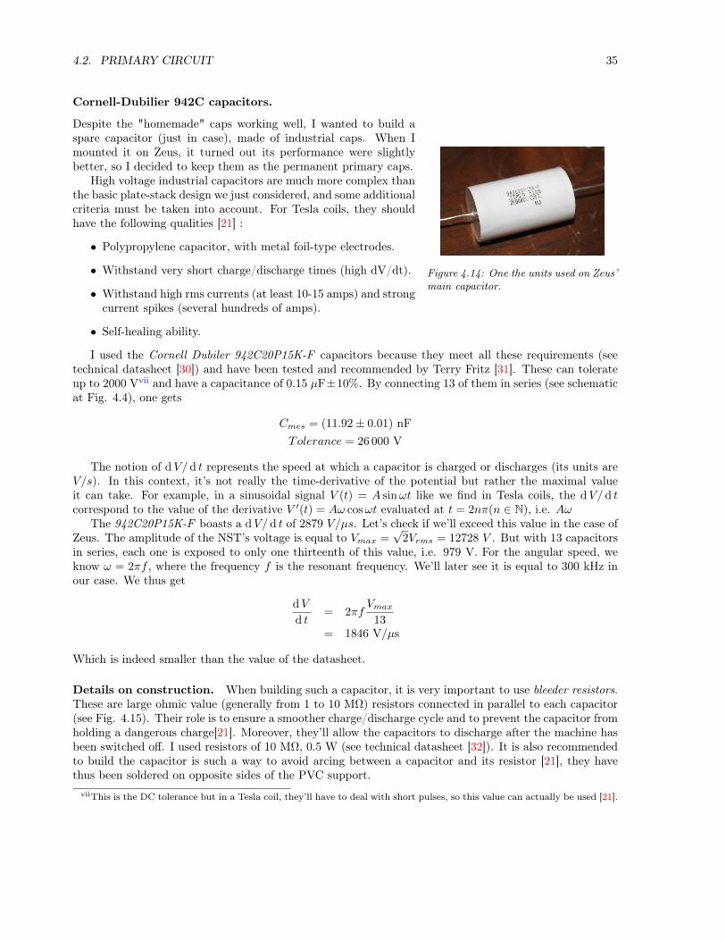
Cornell-Dubilier 942C capacitors.

Figure 4.14: One the units used on Zeus’main capacitor.

Despite the "homemade" caps working well, I wanted to build aspare capacitor (just in case), made of industrial caps. When Imounted it on Zeus, it turned out its performance were slightlybetter, so I decided to keep them as the permanent primary caps.

High voltage industrial capacitors are much more complex thanthe basic plate-stack design we just considered, and some additionalcriteria must be taken into account. For Tesla coils, they shouldhave the following qualities [21] :

• Polypropylene capacitor, with metal foil-type electrodes.

• Withstand very short charge/discharge times (high dV/dt).

• Withstand high rms currents (at least 10-15 amps) and strongcurrent spikes (several hundreds of amps).

• Self-healing ability.

I used the Cornell Dubiler 942C20P15K-F capacitors because they meet all these requirements (seetechnical datasheet [30]) and have been tested and recommended by Terry Fritz [31]. These can tolerateup to 2000 Vvii and have a capacitance of 0.15 µF±10%. By connecting 13 of them in series (see schematicat Fig. 4.4), one gets

Cmes = (11.92± 0.01) nFTolerance = 26 000 V

The notion of dV/ d t represents the speed at which a capacitor is charged or discharges (its units areV/s). In this context, it’s not really the time-derivative of the potential but rather the maximal valueit can take. For example, in a sinusoidal signal V (t) = A sinωt like we find in Tesla coils, the dV/ d tcorrespond to the value of the derivative V ′(t) = Aω cosωt evaluated at t = 2nπ(n ∈ N), i.e. Aω

The 942C20P15K-F boasts a dV/ d t of 2879 V/µs. Let’s check if we’ll exceed this value in the case ofZeus. The amplitude of the NST’s voltage is equal to Vmax =

√2Vrms = 12728 V . But with 13 capacitors

in series, each one is exposed to only one thirteenth of this value, i.e. 979 V. For the angular speed, weknow ω = 2πf , where the frequency f is the resonant frequency. We’ll later see it is equal to 300 kHz inour case. We thus get

dV

d t= 2πf

Vmax13

= 1846 V/µs

Which is indeed smaller than the value of the datasheet.

Details on construction. When building such a capacitor, it is very important to use bleeder resistors.These are large ohmic value (generally from 1 to 10 MΩ) resistors connected in parallel to each capacitor(see Fig. 4.15). Their role is to ensure a smoother charge/discharge cycle and to prevent the capacitor fromholding a dangerous charge[21]. Moreover, they’ll allow the capacitors to discharge after the machine hasbeen switched off. I used resistors of 10 MΩ, 0.5 W (see technical datasheet [32]). It is also recommendedto build the capacitor is such a way to avoid arcing between a capacitor and its resistor [21], they havethus been soldered on opposite sides of the PVC support.

viiThis is the DC tolerance but in a Tesla coil, they’ll have to deal with short pulses, so this value can actually be used [21].


In the same philosophy of extending the caps’ life, it is also recommended to put a small resistance ofa few Ohms in series with the security spark gap. It must have a high power rating, several hundreds ofWatts, and must be non-inductive to avoid the apparition of an extra, parasitic RLC circuit around theprimary capacitor. [21]. I used a 20 Ohms, 100 Watts, thick film-type resistor (see technical datasheet[33]), visible on the left extremity of the brown wire on Fig. 4.16.

Figure 4.15: v.4 during construction. Figure 4.16: v.4 mounted on Zeus’ chassis.

4.2.2 Charge at resonance

Let’s talk briefly about the "good" capacitance of the primary capacitor. In the previous section, wehad chosen its capacity so a resonant amplification occurs at 50 Hz. This ensures all the energy of thetransformer is used, as the impedances of the transformer and the primary circuit are identical. Thischoice is risky however, as in case of spark gap fault, voltage and current rise to enormous values in a fewtens of seconds, which can destroy the caps as well as the transformer.

Figure 4.17: Plot of NST shorted (green) and in primary circuit (blue) output voltage over time in case of resonance(simulation for a 10 kV, 100 mA NST ; L = 318 H ; R = 5000 Ω). [Diagram: Richard Burnett]

The next plot show the maximal values that voltage and current can attain in a primary circuit fed bya 10 kV, 100 mA NST in series with a resonant-sized cap. The ballasts’ inductance is 318 H and the totalresistance is 5000 Ω. We can see that, without a spark gap (or any other device evacuating the energy),voltage can rise up to 200 kV and current up to 2 A [20].


Figure 4.18: Using a resonant-sized capacitor will have the voltage and the current reach values far beyond whatcomponents can withstand. [Diagram : Richard Burnett]

Normally, the spark gap will fire above a given voltage (which is far lower than the previous values),making the current and the voltages across the capacitor fall to acceptable levels. But, for some reason,the spark gap may fail to fire once in a while. This is quite frequent actually, especially for static sparkgaps such as Zeus’ gap, as they have a tendency to fire rather erratically, as show in Fig. 4.19.

Figure 4.19: Plot of the voltage output of the transformer (green) and the voltage across the capacitor (blue) overtime with a static spark gap. This situation depicted here is much more realistic than in Fig. 4.17. [Diagram:Richard Burnett]

Conclusions.

The resonant amplification in the primary circuit is a very important phenomenon for good Tesla coilperformances, but it must remain under control so as not to damage the components. This is why it isstrongly recommended to place security devices around sensitive components.

In this philosophy, a security spark gap is generally placed at the lead of the primary capacitor (visibleon Fig. 4.4). The NST protection filter is a bit more complex and we’ll talk about it later.

It is also recommended to use a non-resonant-sized capacitor, in other words, whose capacitance willnot lead to a brutal resonant amplification. This larger-than-resonance (LTR) value depends on the type


of spark gap used. For a static spark gap, typical values for the LTR capacitance range from 1.5 to 2times the resonant capacitance (given by formula (4.2)) [18]. Kevin Wilson recommends the value of 1.618times the resonant value, as this value (an estimation of the golden ratio), will ensure no common integermultiples [21]. Following this approach, the LTR capacitance of Zeus will be around

CLTR = 14.30 nF

The capacitance of Zeus’ primary caps is approximately 1.35 times the resonant value, which is perhapsa bit close to the resonant value. But the various protection measures seem to be working well as no sensitivecomponent has been damaged (so far).

As mentioned earlier, such an increase in the primary capacity has almost no consequences on the globalperformances of a Tesla Coil. Richard Burnett has shown that, with a static spark gap, the delivered powerdepends much more on the spark gap spacing than on the primary capacity [20].

4.2.3 Inductance

The role of the primary inductor is to generate a magnetic field to be injected into the secondary circuitas well as forming an LC circuit with the primary capacitor. This component must be able to transportheavy current without excessive losses. The resonance tuning is traditionally made on this component aswe’ll see later.

Figure 4.20: Schematic and photograph of Zeus’ primary inductor (secondary circuit removed).

The primary winding has been tapped to 8.25 turns and has a measured self-inductance of

Lmes = (0.03± 0.01) mH

This very approximative value has been measured on a small LCR bridge. A more precise device couldbe used but the tuning is made via a trial-and-error method, so knowing the exact inductance is not ofprime importance.

Different geometries are possible for the primary coil. We’ll look at the most common one beforeexamining more thoroughly the case of Zeus. Note that the formula giving the self-inductances for each ofthem are approximative and are just used to have a rough idea of the number of turns required to achieveproper tuning.


Helical geometry. The inductor looks like a solenoid with widely spaced turns. Such a geometry willcause quite high coupling between the primary and secondary circuits, which is not always a good thingas we discussed in 3.3.5 Influence of the coupling. Apart from the overcoupling problem, having a highprimary increases the risk of arcing between the top load and the primary, which is potentially catastrophic.Indeed, enormous voltages are applied to a circuit that is not designed to handle them, which can leadto destruction of the primary capacitors or/and the transformer if not properly protected. To solve thisissue, the base of the secondary coil can be raised above the primary.

This design has not proven very efficient however [8].

If we call R the radius of the helix, H its height (both in centimeters) and N its number of turns, anempirical formula yielding its inductance L in microhenrys is [9].

Lhelic =0.374(NR)2

9R+ 10H(4.8)

Archimedes’ spiral geometry. This geometry naturally leads to a weaker coupling and reduces therisk of arcing in the primary : it is therefore preferred on powerful coils. It is however rather common inlower power coils for its ease of construction. Increasing the coupling is possible by lowering the secondarycoil into the primary. Zeus’ primary inductor has this shape.

Let W be the spiral’s width given by W = Rmax − Rmin and R its mean radius, i.e. R = (Rmax +Rmin)/2, both expressed in centimeters. If the coil has N turns, an empirical formula yielding its induc-tance L in microhenrys is [9] :

Lflat =0.374(NR)2

8R+ 11W(4.9)

Hybrid geometry. This conical configuration is a sort of compromise. It allow a fair coupling betweenthe two circuits and is rather safe as well. It’s the most common configuration for low power coils. Aposteriori, I think such a geometry would have been a better choice for Zeus, despite being more difficultto built.

By defining the parameters H, W , R and N as previously, the self-inductance is computed by doingan average of the values Lhelic and Lflat weighted by the angle θ of the cone with the horizontal plane[34][9].


Lhybrid =√Lhelic cos2 θ + Lflat sin2 θ (4.10)

Case of Zeus.

Zeus’ primary inductor has a plane spiral geometry, tapped at 8.25 turns. Its internal radius Rmin = 7 cmand its external radius (at 8 turns) Rmax = 44 cm. From here, we find W = 37 cm and R = 25, 5 cmfollowing the previous definition. Its computed inductance is then :

L =0.374(8.25× 25.5)2

8× 25.5 + 11× 37= 27.1 µH

which is close to the measured value. It must be kept in mind however that the primary’s real inductancewill be slightly higher than this value, as the latter neglects the wirings used to connect the components.These wirings indeed form a closed loop which contains some ferromagnetic materials (screws, bolts, etc.).This extra inductance is somewhat wasted as its magnetic field is far from the secondary and will notcontribute to it’s resonance.

Some details must be taken into account in order to keep this parasitic inductance as low as possible.Avoid loops in the wiring and make it as short as possible. It is also recommended to avoid placing wiresparallel to each other to avoid induced currents [35].

Skin effect.

To minimize energy losses, the resistance of the primary circuit must be made as low as possible. Thisimplies the use of good conductors as well as a large conduction area. It is easy to imagine the practicallimitations of this idea. For example, if we wanted to make a spiral from a 12 meter rod of 1.2cm diametermade of massive copper (this is roughly the dimension of Zeus’ primary inductor). This spiral wouldweight 12 kg and would require advanced machinery to be bend. And the cost would be terrific.

Fortunately, we can make use of a propriety of high-frequency currents. The skin effect is the fact that,at high frequencies, the current flow mainly on a thin layer near the outer surface of the conductor viii.We’ll see how this justifies the use of hollow copper tubing (as plumbing pipes), much easier to handle.

Figure 4.21: Alternating current I creates an alternating magnetic field H, which will generate eddy currents Iw.[Illustration: Wikipedia]

Skin effect is easily explained by magnetic induction. When an alternating current flows in a conductor,it will generate a magnetic field around it, which is also alternating. Lenz’ law then says that thesevariations of magnetic field will lead to the apparition of an emf that will tend to attenuate these variations.viiiThis is not rigorously correct actually. The surface of the conductor on which the current will flow will depend on the

ambient magnetic field. For example, in the outer conductor of a coaxial cable, current will flow on its internal surface.


Eddy currents will therefore appear, as shown in Fig 4.21, which will oppose the main current in the centerof the cylinder but not near its edges. When current ~I goes in the opposite direction, so will ~H and ~Iwand the previous discussion holds for both directions.

It can be shown that the current density J(d) in a cylindrical conductor follows an 1/e law from theedges to the center [36] :

J(d) = JSe−d/δ (4.11)

whered is the depth (i.e the distance from the surface),JS the current at the conductor’s surface, JS ≡ J(d = 0),δ is the "skin depth", a parameter depending on the material.

Taking d = δ in (4.11), we see that δ represents the depth at which the current density is only 0.37 (1/e)times the density in the surface. Computing the skin depth is complicated in the general case. However,with a good conductor and at reasonable frequencies (< 1018 Hz), the following formula is a very goodapproximation [36] :

δ =

√2ρ

µω(4.12)

whereρ is the resistivity of the conductor (1.7 · 10−8 Ωm for copper [25])µ is magnetic permeability (1.26 · 10−6 H/m for copper [25])ω the angular speed of the current, equal to 2πf .

Let’s compute the skin depth for copper, the conductor Zeus’ primary inductor is made of, at thefrequency of 300 kHz, its resonant frequency :

δCu ≈ 0.12 mm

We can also calculate the ratio between the current that flows though a plain cylinderand the current that flows into a hollow one. The tubing used for Zeus’ winding is 1mmthick and has a diameter of 12mm.

We find the current I by integrating J(r) over the considered cross-section. We setd = R− r, where R is the cylinder’s radius (6mm) and r the radial distance, which we’llintegrate. We get :

Iplain =

∫ 2π

0

dθ

∫ 6

0

rdr JSe−(R−r)/δ and Ihollow =

∫ 2π

0

dθ

∫ 6

5

rdr JSe−(R−r)/δ

Computing these integrals, we find :

Iplain = 2πJSδ[(r − δ)e(r−R)/δ)

]60

Ihollow = 2πJSδ[(r − δ)e(r−R)/δ)

]65


Figure 4.22: Log-log plot of skin depth δ as a function of frequency f for various mediums. [Diagram: Wikipedia]

We’re only looking at the ratio between the two, to cancel out the unknown factor JS :

IhollowIplain

=

[(r − δ)e(r−R)/δ)

]65[

(r − δ)e(r−R)/δ)]60

=(6− δ)− (5− δ)e−1/δ

(6− δ)− δe−6/δ

≈ 5.8788

5.8800≈ 99.98 %

In other words, the current gain we’d have by using a plain tube is only 0.02%, a ridiculous value. Usinga hollow tubing is therefore perfectly adapted. The drawback of this high-frequency propriety is that theeffective resistance is much higher than in DC, as the current is forced to flow on thin layer instead of onall the conductor (and this, whatever the cross-section of the conductor is) [36].

4.3 Spark gap

The function of the spark gap is to close the primary LC circuit when the capacitor is sufficiently charged,thus allowing free oscillations inside the circuit. This is a component of prime importance in a Tesla coilbecause its closing/opening frequency will have a considerable influence on the final output [37].

An ideal spark gap must fire just when the voltage across the capacitor is maximal and re-open justwhen it falls down to zero. But this is of course not the case in a true spark gap, it sometimes does notfire when it should or continues to fire when the voltage has already diminished ; we’ll see which factorswill make a spark gap efficient.

4.3. SPARK GAP 43

Figure 4.23: Schematic and photograph of Zeus’ (static) spark gap.

Two types of spark gap.

Static. In a static spark gap, there’s two or more electrodes spaced by a given distance. When thepotential difference between them rises above some critical value, the air is ionized and thus becomesconducting. This closes this gap, allowing current to flow.

The critical intensity of the electrical field above which air breakdown occurs depends on many pa-rameters (humidity, temperature, air composition, etc) and it is difficult to predict it in the general case ;gas breakdown itself is a very complex phenomenon. The generally admitted value, which is nothing morethan an order of magnitude, is EC = 3 · 105 V/m [38]. Using this value in the spark gap designix will notyield expected results. Indeed, apart from factors related to air itself, the geometry of the electrodes willinfluence the intensity of the field for a given potential difference as well.

It’s much more efficient to built an adjustable spark gap and to find the optimal distance afterwards,by trial-and-error. This is done by first setting the distance to an obviously too short value, lighting thecoil and observing the result. Next, spacing the gap a little bit and trying again until the arcs at the topload are the longest.

If the electrodes are too close, the gap will fire while the capacitor is not full, which will considerablydiminish the coil performances. If they are too distant, the spark will simply not fire and the coil doesn’twork. The latter case is much more dangerous as we discussed in section 4.2.2 Charge at resonance. If theprimary circuit is correctly conceived however, the security gap will take over and will bypass the fragilecomponents.

Static spark gaps are easy to construct but generally have poorer performance than their rotating coun-terpart [37]. They have a tendency to fire erratically and to carry on firing when voltage has diminished.Moreover, the path of ionized air has a certain resistance.

Rotative. On this kind of spark gap, it’s no longer the voltage that closes the circuit. Here, we havebasically a conducting rod that spins rapidly between electrodes. When the rod is at its closest distancefrom the electrodes, current flows via small paths of ionized air. When the rod offsets from this position,current flow stops, which re-opens the gap.

There are many ways to built such a rotative gap (several rods, several pairs of electrodes, synchronousor asynchronous motor, etc.).

This kind of spark gap is more precise and yields better results, but is more difficult to build andadjust. Indeed, it must be built in such a way so the rod passes in front of the electrodes just when the

ixFor example, setting the inter-electrode distance to 1 cm, hoping breakdown will occur when the potential differencebetween them will reach 30 000 V


voltage difference across the capacitor is maximum.

Details about construction.

Zeus’ spark gap is a static one. As mentioned earlier, they tend to remain open after the voltage hasdiminished. This happens because the path of ionized air demands a much lower voltage to live on thanit requires to be created.

Figure 4.24: Heavy corrosion betweenthe copper tubes.

In order to improve its performances, the gap has to bequenched, that means to be forced open. Here’s a few strategiesfor that.

One is to force a large, continuous flow of air inside the sparkgap, in order to chase the ionized air. Sucking the air is also possible(for example, with vacuum cleaner parts) and gives good results aswell[39].

Blowing air into the gap has many benefits. This not onlyquenches the gap but also cools it. Because the critical breakdownfield decreases with temperature and the high current crossing thespark gap will indeed increases its temperature, the spark gap willfire at a lower voltage after a few seconds (and the sound of thespark gap becomes notably more high-pitched), hindering the coilsperformances [37]. Thus cooling the gap will prevent such prob-lems.

It is also possible to use more than two electrodes. The singlearc will then be divided into so many smaller arcs, which will quench more easily. The drawback of thisconfiguration is that all these sub-arcs will act like series resistors : all of them will dissipate energy inthe form of light, heat and noise. The Richard-Quick design makes use of several copper tubes disposedin parallel [40]. I used this model for Zeus’ gap.

The spark gap has to deal with enormous current, with transient spikes of nearly 300 amperes. Thisleads to the apparition of strong corrosion on the electrodes, which will also hinder the coils performances.It is necessary to regularly clean/sand them.

1st version. The first spark gap I built was made of 5 identical copper tubes, 10mm in diameter, 80mmlong. These were fixed on a flexible membrane following a design found on ref. [41]. By bending thismembrane, one can modify the distance between the electrodes. The whole assembly was placed in frontof a 12 V personal computer fan with a diameter of 80mm. Power was supplied by two 9V batteriesconnected in series.

Figure 4.25: v.1 mounted on Zeus’ chassis.

4.4. SECONDARY CIRCUIT 45

The membrane must be made of an insulting, fire-resistance material. I used foamed PVC, which isauto-extinguishable. Its flexibility was not excellent however and didn’t allow a good distance setting. AsI tried to bend it more, it eventually broke.

This spark gap was not easy to maintain either. The repeated action of sanding the surfaces had atendency to loosen the fixations of the tubes. A better design was to be found.

2nd version. This spark gap was made of the same copper tubes as before. The difference here is themounting. The tubes are loosely fixed at both extremities on PVC supports. The support close to thefan was immobile while the other could be horizontally translated (the magnet on metal bar ensured thestability of the assembly).

The spacing between the tube can thus be adjusted by shearing the assembly. This design proved moreprecise and easy to maintain.

Figure 4.26: v.2 mounted on Zeus’ chassis. Figure 4.27: The power supply of the fan.

4.4 Secondary circuit

4.4.1 Coil

The function of the secondary coil is to bring an inductive component to the secondary LC circuit and tocollect the energy of the primary coil.

This inductor is an air-cored solenoid, generally having between 800 and 1500 closely wound adjacentturns. In the Zeus Tesla coil the secondary coil is made of enameled copper "magnet wire" with a diameterof 0.5mm (SWG 24) which is wound around a PVC pipe of 100mm external diameter. The coil is 40.2cmtall.

To calculate the number of turns that have been wound, this quick formula will avoid a certain fastidiouswork:

N = H/d (4.13)

where H is the height of the coil and d the diameter of the wire used. In our case, the number of turnsis 790 turns (more or less a few turns). It is quite low, but the diameter of the coil is rather large incomparison of the coil’s power ; this will provide a fair self-inductance while limiting parasitic capacity.

Another important parameter is the length l we need to make the entire coil. It is given by

l = 2πNr (4.14)


Figure 4.28: Schematic and photograph of Zeus’ secondary coil.

where r is the radius of the coil. Zeus’ coil has thus necessitated 248 meters of wire.One can show that the self-inductance L in henrys of a adjacent-turns solenoid is given by

L = µN2A

H(4.15)

where µ represents the magnetic permeability of the medium (≈ 1.257 · 10−6 N/A2 for air, very close tothe value of the void), N the number of turns of the solenoid, H its total height, and A the area of a turn.

Injecting Zeus’ coil values, we getLth = 15.17 mH (4.16)

which is not too far from the value measured from an LCR bridge :

Lmes = (11.92± 0, 01) mH (4.17)

Characteristics

Resistance. During the first tries of Zeus, I had placed the secondary coil lower in the primary spiralin order to increase coupling. This didn’t yield the expected results : arcing between the primary andsecondary occurred, which damaged the coil at several points, as shown in Fig. 4.29. I thus put thesecondary coil back in its initial position. Fortunately, the coil hasn’t been sectioned. The only noticeableconsequence was an increase of the coil’s resistance, increasing from 20 to 25 Ohms.

However, this value was measured with a classical ohmmeter, i.e. with a direct current. But what willflow in the coil is high-frequency alternating current. A more precise measure would include effects suchas skin effect and proximity effect. The method proposed by Fraga, Prados and Chen [42] takes theseeffects into account and has been proven to be precise for solenoids. The JAVATC simulator yielded thefollowing value ("Fraga AC resistance") :

Rac = 94.856 Ω


Figure 4.29: Results of inadequate space between the coils : arcing between the two occurred, burning the secondarycoil at several points.

Inductance and capacitance at resonance. The inductance calculated at (4.16) and measured at(4.17) are again valid for low frequencies only. The self inductance of the secondary coil driven at resonanceis slightly different, because of the non-uniform repartition of current and because the length of the coil iscomparable to the wavelength of the signal it will carry [43]. Once again, a more precise formula must beused. The JAVATC simulator gave the following value ("Effective series inductance") :

Lres = 13.471 mH

It’s also interesting to know the (parasitic) capacitance of the coil [44]. Here also the formula iscomplicated in the general case. We’ll use the value yielded by JAVATC ("Effective shunt capacitance"without top load) :

Cres = 6.74 pF

Q factor. We can now compute the Q factor of the coil, following formula (3.51) established in the lastchapter, Q = R−1

√L/C. To get a coherent result, we’ll use the previous values for R, L and C (with top

load capacitance added). We thus get :Q = 285

Which is a rather good value, that will indicate low losses in the secondary LC circuit. It is difficult tosurpass 500 with common conductors.

Note that it is also possible to measure the Q factor experimentally following the procedure detailedin ref. [45].

Quarter-wave antenna.

We saw in section 3.4 Quarter-wave antenna how we could apply this model to the Tesla coil. In the nextsection, we’ll calculate the resonant frequency f of the secondary coil to be 3.19·105 Hz. The correspondingwavelength is λ = c/f (where c is the speed of propagation of the wave : here, c ≈ 2.998 · 108 m/s), i.e.approximately 940 m. In other words,

λ/4 = 235 m

As the total length of the wire in Zeus’ secondary coil is around 248 meters, we can conclude it iscorrectly tuned like a quarter-wave antenna. But as mentioned earlier, this is not necessary [8], that iswhy we performed such rough calculationsx.

xActually, we should have used the speed of propagation of the wave in copper for c, instead of the vacuum, but bothvalue are actually rather close [15].


Construction.

This component is not especially difficult to build but requires a lot of patience. The 800 turns have beenwound entirely by hand and took a few days. Precautions had to be taken in order to prevent sweat frominfiltrating the coil.

The very high voltages involved can cause arcing between turns if the coupling is set too high xi. Itis common to apply an insulating resin on the coil, which will reinforce the insulation already providedby the polyurethane covering the magnet wire. I couldn’t find such a resin so I instead applied liberalamounts of insulating spray (the same used in the capacitors).

There’s an important empirical rule about the ratio between the height H and the diameter D of thecoil. It has been observed that the best performances are attained with an H/D ratio between 3 and 5[46][47]. Zeus’ coil is thus conform with a ratio of 4 (see Fig. 4.28).

Figure 4.30: "Keep calm and carry on."

4.4.2 Top loadThe top load acts like the upper "plate" of the capacitor formed by the top load and the groundxii. Itadds capacity to the secondary LC circuit and offers a surface from which arcs can form. It is possible,actually, to run a Tesla coil without a top load, but performances in terms of arc length are often poor, asmost of the energy is dissipated between the secondary coil turns instead of feeding the sparks[7].

The are many different possibilities regarding the shape of the top load, the most common ones beingthe sphere and the toroid. Computing its capacitance is difficult in the general case (a collection ofempirical formulas are given in ref. [13]). The JAVATC program gave the next value :

Cs = 14.172 pF

Influence of geometry.

The top load is perhaps the most important component when determining the final arc length (except thetransformer of course). There is a lot of discussion about its optimal size.

In a general way, a larger top load will have a larger capacitance. Regarding formula (3.57) specifyingthe voltage gain, one could think it is desirable to keep the secondary capacitance as low as possible, as Voutdecreases when Cs increases. However, if the top load capacitance is low (or nonexistent), the majority

xiSee 3.3.5 Influence of coupling.xiiSee 3.3.4 Distribution of capacitance in the secondary circuit.


Figure 4.31: Schematic and photograph of Zeus’ top load

(resp. the totality) of the secondary capacitance will be located in the secondary coil itself. Then, theenergy of the secondary circuit is mainly dissipated as heat between the turns instead of feeding the sparks[7]. Hence an optimal capacitance exists.

The toroidal geometry is often preferred instead of the spherical. If the top load is a sphere, the nearelectrical field will be more uniform, which will result in more numerous, shorter sparks. But with atoroidal geometry, the electrical field is more intense on the outer edge of the toroid : there will be fewersparks but longer on average, most of the arising form this outer edge.

Be it toroidal of spheric, the curvature radius of the load will increase with its size. And the largerthe curvature radius is in a certain zone, the weaker the electric field will be. Fewer spark will be ableto form, and the available energy for each of them will be greater. This will result in less numerous butlonger sparks. It is even possible to make the top load big (and smooth) enough so not a single arc canform [48]. Conversely, if the curvature radius is smaller, the electrical field will be intense in many zones,allowing more sparks to be formed ; these will be shorter as the available energy will have to be distributedbetween all these arcs. There is thus also an optimal size to the top load.

State of the surface. Another important parameter influencing the final arc length is the roughness ofthe top load surface. If the surface has asperities, the electric field near these will be much more intense. Itcan indeed be shown from Maxwell’s equations (Gauss’ law to be precise) that the electrical field is moreintense near zones of strong curvature. This fact is called the spike effect.

If one wishes to get longer sparks, it will be judicious to have a smooth top load ; to reduce the numberof breakout points and thus of sparks (see for example ref. [49]).

Addition of a breaking point. In order to force sparks to be generated at a single point (and thushaving longer arcs), it is possible to add a breaking point to the top load. By spike effect, this will ensurethe electrical field is comparatively much stronger near this zone.

It has been suggested that the breakout point should be a ball instead of a spike. This will allow thespark base to "glide" on it, giving more time for the spark to developxiii. Because of the higher temperatureof the ionized air path, it will indeed have a tendency to rise.

Details of construction.

xiiiSee 3.3.1 Description of a cycle.


Figure 4.32: Numerous sparks arising from the top load asperities. Notice Zeus’ Eagle. 1s shutter speed.

A toroidal top load was used on Zeus.There are a few empirical rules regarding the dimension of the toroid. Let’s

call d its minor diameter and D its major diameter, like shown in adjacent figure.d should be equal to the secondary coil diameter (10cm here) and the D/d ratioshould be between 3 and 4.

The top load position is also subject to some guidelines. If it is too close fromthe top of the secondary coil, its electrical field will "drown" the last spires, whichwill result in a lower final voltage. Conversely, if the top load is too high, itselectrical field cannot protect the last spires and the risk of inter-arc spark andCorona losses increases. If we call h the distance between the base of the top loadand the top of the secondary coil, it is recommended to have d ≈ h[49].

Figure 4.34: The very first sparks ofZeus. A lot of emotion. 1s shutter speed.

1st version. The first toroid I made had a minor diameter d =8 cm and a major diameter D = 28 cm. Its theoretical capacitancewas 13.5 pF.

It was made of flexible aluminum duct. It has been rolledaround a support made of two discs, one in wood (top) and theother in aluminum (bottom). The toroid was closed with aluminumtape.

The connection with the secondary coil was made with a lusterconnector. On the next picture, one can spot a small Corona "leak"at this point because of the roughness of the screws.

This toroid produced the very first sparks of Zeus. Their sizewas modest, because of the capacity of the top load was too low. To enhance performances, Kevin Wilsonsuggested to build a new, larger toroid.

2nd version. This is the final version of Zeus’ toroid. The same construction method was used, onlydimensions changed : d = 10 cm, D = 35 cm. The rod serving as a breakout point is attached with a

4.5. RESONANCE TUNING 51

Figure 4.33: Adding a spike forces the sparks to break from a single point, to a certain extent. Their length alsoincreases. 3.2s shutter speed.

neodymium magnet. Fig. 4.33 attests of the great difference between the two top loads in terms of arclength.

I just had to retune the primary inductance in order to make the two circuits resonate. We’ll discussthis point in the next section.

4.5 Resonance tuning

Setting the primary and secondary circuits at resonance, i.e. have them share the same resonant frequency,is of prime importance for good operation. As discussed in 3.2 LC circuit, the response of an RLC circuitis the strongest when driven at its resonant frequency. In a good RLC circuit, the response intensity fallssharply when the driving frequency drifts from the resonant value.

Let’s have a look at Zeus’ case. We compute the secondary resonant frequency with its capacitance Csand its inductance Ls with the well-know formula (3.46), f = (2π

√LsCs)

−1. The secondary capacitanceis equal to the coil capacitance plus the top load capacitance, computed by taking into account the non-uniformity of the current distribution. But the non-uniformity of the current distribution[44]. The JAVATCsimulator gives a value for the total secondary capacitance (Effective shunt capacitance), Cs = 18.425 pF.Let’s also recall the secondary inductance : Ls = 13.471 mH.

We thus getfres = 319.46 kHz

Tuning methods.

The tuning is generally done by adjusting the primary inductance, simply because it’s the easiest compo-nent to modify. As this inductors has wide turns, it is easy to modify its self-inductance by tapping thefinal connector at a certain place in the spiral.

The simplest method to achieve this adjustment is by trial-and-error. For this, one begins to tap theprimary at a point supposedly close to the resonant one, lights the coil and evaluates arc length. Thenthe spiral is tapped a quarter of turn forward/backward and one re-evaluates the result. After a few triesone can proceed with smaller steps, and will finally get the tapping point where the arc length is the


Figure 4.35: Because of the non-ideal behavior of the components, the secondary circuit can exhibit more than oneimpedance minimum. [Diagram: Jamie Oliver]

highest. Normally, this tapping point will indeed set the primary inductance such as both the circuits areat resonance. I used this procedure for Zeus and tapped the primary to 8.25 turns.

This method isn’t infallible however. It presupposes that there is one and only one resonant point.This would be true if current and voltage distribution were uniform. And we saw the secondary coil hasa distributed capacitance and deals with non-uniform current/voltage distributions. This may lead to theapparition of several secondary resonances (see Fig. 4.35), i.e local but not necessarily global impedanceminima [50]. By proceeding though the trial-and-error method discussed above, one can think they’vereached the true resonant value but actually have a secondary resonance.

A more precise method would involve an analysis of the individual response of both the circuits (in thecoupled configuration, of course, i.e. without physically separating the circuits) with a signal generatorand an oscilloscope. Detailed procedure are given in refs. [51] [50].

Arcs themselves can produce some extra capacitance [14]. It is therefore advised to set the primaryresonant frequency slightly lower than the secondary, in order to compensate for this. This is noticeablehowever only with powerful Tesla coil (which can produce arcs longer than 1m), and should have littleinfluence on Zeus.

4.6 RF ground

Figure 4.36: Zeus’ RF ground is made of an 1 squared meter aluminum plate.

It is the ground at which the bottom of the secondary coil is connected. Its role is to keep the voltageat the base of the coil at zero, but also (more importantly) to act like the second "plate" of the topload-ground capacitor. In this light, it makes the secondary capacitance less dependent of the immediateenvironment.

4.7. OTHER COMPONENTS 53

The best grounding method is to use a metallic rod stuck into the soil ; when this option is notpossible, one has to make his own ground. For this purpose, it is possible to use a large metallic plate,placed underneath the Tesla coil. Its total width should be equal to twice the distance between the topload and the base of the secondary coil [52]. Zeus being 1.10m high, a plate 2.2m wide would be required.The plate used on Zeus is only 1m wide but seems to be sufficient. It is made of 4 panels of 50cm × 50cmbound with aluminum tape and covered by stronger, convectional tape for protection. This allow the plateto be folded, which increases transportability.

Zeus’ plate is made of plain metal, but it is also possible to use a conducting mesh. This is actuallybetter as it prevents some eddy current from taking place.

4.7 Other components

4.7.1 NST protection filter

Tesla coils give a harsh treatment to the main transformer. We saw that it must withstand powerfultransient currents and voltages as well as high-frequency alternating current. To ensure long transformerlife, it is highly recommended to protect it. We mentioned earlier that it is not possible to use a differentialcircuit breaker as it will open the circuit as soon as resonant amplification attains higher values, thusforbidding any Tesla coil use.

Terry Fritz has however designed an NST protection filter specifically made for Tesla coil operation[53]. It is made of a grounded spark gap, low-pass filters and varistors and is connected between thetransformer and the primary circuit. Such a filter has been used on Zeus.

Note that a filter is necessary only with NSTs, because of their fragility. Other kinds of transformers(MOT, pole pigs, etc) are rugged enough to support Tesla coil operation as is [54].

Figure 4.37: Schematic and photograph of Zeus’ NST protection filter (wires not yet present).

Spark gap. It is made of three electrode (or four, a pair per side), the central one being connected toground. If a voltage spike occurs, the gap fires and the dangerous current is redirected to ground, thussparing the transformer.


RC low-pass filter. It is physically just behind the spark gap and is made of a 1000 Ω, 100 W ceramicresistor (technical datasheet : [55]) and of 6 high-voltage capacitors of 3.3 nF each (technical datasheet :[56]), thus totalizing 0.55 nF. Here also, bleeder resistor were soldered in parallel of each capacitorxiv.Atthe beginning, there was an arcing problem between these resistors and the wooden support on which theylied, but a PVC support solved the issue.

The resistors cause very little energy loss as the current is very weak (25 mA rms). The average lossP is given by P = RI2 = 0.25 W, which is really negligible in comparison of the 225 watts supplied. Notealso that they help preventing the current flowing into the primary to come back into the transformer andbeyond. Indeed, the impedance of the main spark gap firing is negligible in front of the total impedanceof the NST and the filter : when it fires, it almost short-circuit these components and the high primarycurrents stay where they are.

In sinusoidal regime, the cutoff frequency of a low-pass filter is the frequency above which the trans-mitted intensity will be less than 0.707 (

√1/2) times the input intensity [57]. One can show it is given

by:

fc =1

2πRC(4.18)

We thus find the cutoff frequency to be around 287 kHz. The filter will therefore further help block theprimary currents (around 320 kHz for Zeus), but more importantly, they will block the interferences ofmuch higher frequencies (see ref. [7], Frequency splitting).

Varistors. Metal oxide varistors (MOVs) complete the protection filter. These non-linear componentshave their resistance drop dramatically above a certain voltage. Here, this threshold is 1800 V in directcurrent and 1000 V in alternating current (technical datasheet: [58]). As there are 7 of them on each side,the total threshold voltage is 7000 V. The voltage difference between a wire and the ground is 4500 V rms,so the amplitude is 6364 V, which is just below the threshold.

These components help to protect the NST from voltage spikes in case the spark gaps don’t fire.Actually, they’re not strictly necessary.

Ground. The central wire of this filter should not be connected to the safety ground. Voltage and currentspikes as well as high-frequency interference would be sent, which is hazardous for electronic apparatusesconnected to the mains.

A proper ground for this filter is the soil.

4.7.2 PFC capacitorThe power average over a period T of an alternating current is defined as following :

< P >=1

T

∫ T

0

V (t)I(t) d t (4.19)

where current and voltage are definition by sinusoidal functions of same frequency, but whose amplitudeand phase can change. One can easily prove the next result :

1

T

∫ T

0

cos (ωt− φ) cos (ωt− ψ) d t =1

2cos (φ− ψ) (4.20)

We thus see that the power is maximum when voltage and current are in phase.The high self-inductance of the transformer causes the current to lag the voltage, which results in less

transmitted power as we just saw. To overcome this problem, i.e. re-phase both signal, one connects acapacitor in parallel to the transformer inputs. In a capacitor, it is indeed the voltage that is delayed withrespect to current. This is the role of the power factor correction capacitor (PFC cap).xivThe same ones used in the primary capacitor, see 4.2.1 Capacitors - Cornell-Dubilier 942C.

4.7. OTHER COMPONENTS 55

Figure 4.38: The protection filter assembled. The NST is in the wooden box just under the filter.

Figure 4.39: Zeus’ PFC cap.

This capacitor must be able to work continuously, i.e. must be a run-type capacitor. The start-typecapacitors on the other side are designed to work only during short time intervals .

One can show the ideal capacitance of the PFC cap is given by [59]:

CPFC =P

2πfV 2in

(4.21)

whereP is the transformer power,f is the mains frequency (50 Hz in Europe),Vin is the mains voltage (230 V).

This yiels a value of 13.54 µF for Zeus. The capacitor used is 12 µF (technical datasheet : [60]). Havingthe exact value doesn’t matter as long as they are close enough [59].


4.7.3 AC line filter

In order to protect the electronic devices connected to the mains from dangerous transient currents/voltagesand from radio interferences generated by the Tesla coil circuits, it is recommended to connect a last filterbetween the mains and the transformer.

Figure 4.40: Schematic and photograph of Zeus’ EMI filter.

Those interferences are normally blocked by the NST protection filter, but it is perhaps not a goodidea to fully rely on a DIY component to protect the home electrical installation.

It is advised to place it as far as possible from the Tesla coil to avoid the apparition of induced currentabove the filter, hence reducing its effectiveness [61].

4.8 Last step

Figure 4.41: The machine’s brass plate lies on the wooden support of the switch.

Chapter 5

Nikola Tesla, a mind ahead of its time.

This last chapter is left to Nikola Tesla, with these few quotes I find inspiring and that depicts his way ofthinking.

"It is a mere question of time when men will succeed in attaching their machineryto the very wheelwork of nature."

(Experiments with Alternate Current of High Potential and High Frequency, 1892)

"The scientific man does not aim at an immediate result. He does not expect that his advanced ideas willbe readily taken up. His work is like that of the planter - for the future. His duty is to lay the foundation

for those who are to come, and point the way. He lives and labors and hopes."(Radio Power Will Revolutionize the World, in Modern Mechanics and Inventions, 1934)

"I have obtained... spark discharges extending through more than one hundred feet and carrying currentsof one thousand amperes, electromotive forces approximating twenty million volts, chemically active

streamers covering areas of several thousand square feet, and electrical disturbances in the natural mediasurpassing those caused by lightning, in intensity.

Whatever the future may bring, the universal application of these great principles is fully assured, thoughit may be long in coming. With the opening of the first power plant, incredulity will give way to

wonderment, and this to ingratitude, as ever before."(A means for furthering peace, 1905)

57

58 CHAPTER 5. NIKOLA TESLA, A MIND AHEAD OF ITS TIME.

Figure 5.1: Tesla reading Theoria Philosophiae Naturalis,in front of the coil of its high-frequency transformer, EastHouston Street, New-York. [Photograph : Wikimedia Commons]

Appendices

59

Appendix A

Specifications of the Zeus Tesla coil

This appendix lists the inputs and outputs of the JAVATC simulations regarding the proprieties of theindividual components.

J A V A T C version 13.0 - CONSOLIDATED OUTPUTlundi 5 mars 2012 2:08:49

Units = CentimetersAmbient Temp = 20 Celsius

----------------------------------------------------Secondary Coil Inputs:----------------------------------------------------Current Profile = G.PROFILE_LOADED5 = Radius 15 = Radius 20 = Height 140.2 = Height 2790 = Turns0.0508 = Wire Diameter

----------------------------------------------------Primary Coil Inputs:----------------------------------------------------Round Primary Conductor7 = Radius 125 = Radius 20 = Height 10 = Height 28.25 = Turns1.2 = Wire Diameter0.01192 = Primary Cap (uF)30 = Total Lead Length0.5 = Lead Diameter

----------------------------------------------------Top Load Inputs:----------------------------------------------------Toroid #1: minor=10, major=36, height=50, topload

----------------------------------------------------Secondary Outputs:----------------------------------------------------

60

61

319.46 kHz = Secondary Resonant Frequency90 deg = Angle of Secondary40.2 cm = Length of Winding19.65 cm = Turns Per Unit0.00086 mm = Space Between Turns (edge to edge)248.19 m = Length of Wire4.02:1 = H/D Aspect Ratio20.939 Ohms = DC Resistance27039 Ohms = Reactance at Resonance0.447 kg = Weight of Wire13.471 mH = Les-Effective Series Inductance14.185 mH = Lee-Equivalent Energy Inductance13.831 mH = Ldc-Low Frequency Inductance18.425 pF = Ces-Effective Shunt Capacitance17.498 pF = Cee-Equivalent Energy Capacitance28.809 pF = Cdc-Low Frequency Capacitance0.1243 mm = Skin Depth14.172 pF = Topload Effective Capacitance94.8557 Ohms = Effective AC Resistance285 = Q

----------------------------------------------------Primary Outputs:----------------------------------------------------317.15 kHz = Primary Resonant Frequency0.72 % high = Percent Detuned0 deg = Angle of Primary829.38 cm = Length of Wire1.26 mOhms = DC Resistance0.982 cm = Average spacing between turns (edge to edge)1.375 cm = Proximity between coils2.31 cm = Recommended minimum proximity between coils20.842 uH = Ldc-Low Frequency Inductance0.01175 uF = Cap size needed with Primary L (reference)0.284 uH = Lead Length Inductance74.074 uH = Lm-Mutual Inductance0.138 k = Coupling Coefficient0.129 k = Recommended Coupling Coefficient7.25 = Number of half cycles for energy transfer at K11.29 us = Time for total energy transfer (ideal quench time)

----------------------------------------------------Transformer Inputs:----------------------------------------------------230 [volts] = Transformer Rated Input Voltage9000 [volts] = Transformer Rated Output Voltage25 [mA] = Transformer Rated Output Current50 [Hz] = Mains Frequency230 [volts] = Transformer Applied Voltage

----------------------------------------------------Transformer Outputs:----------------------------------------------------225 [volt*amps] = Rated Transformer VA360000 [ohms] = Transformer Impedence9000 [rms volts] = Effective Output Voltage0.98 [rms amps] = Effective Transformer Primary Current0.025 [rms amps] = Effective Transformer Secondary Current225 [volt*amps] = Effective Input VA0.0088 [uF] = Resonant Cap Size0.0133 [uF] = Static gap LTR Cap Size0.0231 [uF] = SRSG LTR Cap Size

62 APPENDIX A. SPECIFICATIONS OF THE ZEUS TESLA COIL

14 [uF] = Power Factor Cap Size12728 [peak volts] = Voltage Across Cap31820 [peak volts] = Recommended Cap Voltage Rating0.97 [joules] = Primary Cap Energy304.4 [peak amps] = Primary Instantaneous Current55.1 [cm] = Spark Length (JF equation using Resonance Research Corp. factors)12 [peak amps] = Sec Base Current

----------------------------------------------------Static Spark Gap Inputs:----------------------------------------------------5 = Number of Electrodes1.5 [cm] = Electrode Diameter0.4 [cm] = Total Gap Spacing

----------------------------------------------------Static Spark Gap Outputs:----------------------------------------------------0.1 [cm] = Gap Spacing Between Each Electrode12728 [peak volts] = Charging Voltage12450 [peak volts] = Arc Voltage36966 [volts] = Voltage Gradient at Electrode31125 [volts/cm] = Arc Voltage per unit97.8 [%] = Percent Cp Charged When Gap Fires10.09 [ms] = Time To Arc Voltage99 [BPS] = Breaks Per Second0.92 [joules] = Effective Cap Energy324949 [peak volts] = Terminal Voltage92 [power] = Energy Across Gap58.6 [cm] = Static Gap Spark Length (using energy equation)

Program written by Barton B. Anderson ; http://www.classictesla.com/java/javatc/javatc.html

Appendix B

Behavior of the signal in the secondarycoil

This appendix presents the results of the JAVATC simulation regarding the behavior of voltage and currentas a function of height in the secondary.

Voltage and Current distribution along the length of the secondary coil.

Length Voltage Current0.00 0.00 11.80.3 1755.8 11.91 5815.6 11.92.5 15548.3 124 26395.5 125.4 37913.8 126.9 49857.5 128.4 62077.7 129.8 74477.9 1211.3 86992.7 11.912.8 99575.5 11.914.2 112191.4 11.915.7 124813 11.817.2 137417.8 11.818.6 149986.4 11.720.1 162501.6 11.721.6 174947.2 11.623 187307.6 11.524.5 199566.7 11.426 211707.5 11.327.4 223710.5 11.228.9 235553.2 11.130.4 247206.9 1131.8 258633.7 10.933.3 269780.3 10.834.8 280567.8 10.736.2 290872.9 10.537.7 300491.1 10.439.2 309046 10.339.9 312588.3 10.140.2 314120.8 10

Program written by Barton B. Anderson ; http://www.classictesla.com/java/javatc/javatc.html

63

64 APPENDIX B. BEHAVIOR OF THE SIGNAL IN THE SECONDARY COIL

Distribution du voltage

0

50000

100000

150000

200000

250000

300000

350000

0 5 10 15 20 25 30 35 40 45

Hauteur dans le secondaire [cm]

Vo

ltag

e [V

]

Distribution du courant

9,5

10

10,5

11

11,5

12

12,5

0 5 10 15 20 25 30 35 40 45

Hauteur dans le secondaire [cm]

Co

ura

nt

[A]

Figure B.1: Plots of the previous values.

Appendix C

Analysis of the RLC circuit

We propose here to make a quick mathematical analysis of the series RLCcircuit with a sinusoidal voltage generator, like the one on the next figure.We will make more precise some of the qualitative explanations of section3.2.3, and also generalize the results obtained for the LC circuit.

The equation describing this system is different from equation (3.24) ofthe LC circuit because of the added resistor R. The tension across the leadsis given by Ohm’s law (3.1) V = RI. Using Kirchoff’s law for currents, weknow that the current I(t) is identical in the entire loop. We then have :

LI +RI +1

C

∫I dt = V0 sin Ωt (C.1)

or in a equivalent way :

LQ+RQ+1

CQ = V0 sin Ωt (C.2)

where we used the relation I = dQdt .

Underdamped case : 0 < R2L <

1√LC

.

Homogeneous solution. We first look at the situation where there’s no driving force. We begin bysetting the following two quantities, which both have the dimensions of an angular speed :

α =R

2L

ω =1√LC

(C.3)

Equation (C.2) thus readsQ+ 2αQ+ ω2Q = 0 (C.4)

By resolving this equation with the characteristic polynomial method, one finds :

Qh(t) = e−αt[Q0 cos ωt+

(I0 +Q0α

ω

)sin ωt

]with ω =

√ω2 − α2

(C.5)

65

66 APPENDIX C. ANALYSIS OF THE RLC CIRCUIT

where Q0 and I0 respectively represent the charge and the current at the initial moment t = 0.In this free regime, we see that the system carries out oscillations whose amplitude exponentially

decrease with time, conversely to the LC circuit where the oscillation amplitude stays constant. We alsoremark that the natural pulsation of the oscillations ω has "shifted" from the LC’s one (page 9), whichwas ω = 1/

√LC. Finally, we notice that at the limit where the attenuation term α goes to 0, we recover

the solution for the LC circuit (formula (3.22), where we moreover set I0 = 0).One finds the current I(t) by derivating (C.5) with respect to time.

General solution. One can verify that the following function is indeed a particular solution to (C.1) :

Qp(t) = V0−2αΩ sin Ωt+ (ω2 − Ω2) cos Ωt

(ω2 − Ω2)2 + 4Ω2α2(C.6)

The general solution is therefore :

Q(t) = e−αt[Q0 cos ωt+

(I0 +Q0α

ω

)sin ωt

]+ V0

−2αΩ sin Ωt+ (ω2 − Ω2) cos Ωt

(ω2 − Ω2)2 + 4Ω2α2(C.7)

Here we see that the term 4Ω2α2 prevents the asymptotic behavior encountered in the LC circuit whenΩ = ω : Oscillations remain bounded no matter what in an RLC circuit. This explains the differencesbetween Figs. 3.9 and 3.11. An important thing to note is that, beside the frequency of the free oscillationsof an RLC circuit ω =

√ω2 − α2 is different from the LC circuit, the resonant frequency in driven regime

remains the same : the last term of (C.7) is maximal when Ω = ω and not ω. This is why the results onresonant frequency derived for the unrealistic LC circuit still holds for Tesla coil circuits.

Current I(t) can be found by time-derivating (C.7).

Overdamped case 0 < 1√LC

< R2L .

Now the attenuation term α is greater than the oscillating term ω, the discriminant of the characteristicpolynomial of (C.1) is positive and the solution is a sum of real exponentials instead of imaginary ones.The particular solution (C.6) is unaffected by this change however. Let’s directly write down the generalsolution then :

Q(t) = e−αt[Q0 cosh ωt+

(I0 +Q0α

ω

)sinh ωt

]+ V0

−2αΩ sin Ωt+ (ω2 − Ω2) cos Ωt

(ω2 − Ω2)2 + 4Ω2α2(C.8)

The only oscillations the circuit executes come from the driving force, without which no oscillations wouldtake place.

Case where 1√LC

= R2L .

There is in theory a third situation, said to be critically damped, that account for 1√LC

= R2L . This

intermediate situation is very rare in practice. The characteristic polynomial has an unique root and thehomogeneous solution thus reads:

Qh(t) = (K1 +K2t)e−ωt (C.9)

where K1 et K2 are integration constants than can be determined in terms of the initial conditions.

See also• Ron Cummings, College of the Redwoods, RLC Circuit, 1997,http://online.redwoods.cc.ca.us/instruct/darnold/deproj/Sp97/Ron/ronproj.pdf.

http://online.redwoods.cc.ca.us/instruct/darnold/deproj/Sp97/Ron/ronproj.pdf

Appendix D

Analysis of two inductively coupledoscillating circuits.

Let’s make a short analysis of the system made of two inductively coupled oscillating circuits. We’ll firstdeal with two coupled LC circuits, and then two RLC circuits. The goal is to look at the differentialequations that describe the behavior of the Tesla coil itself relatively well.

We will only look at the homogeneous cases, as when the spark gap fires, the alternating voltagegenerator (i.e. the transformer) is almost short-circuited.

D.1 Two coupled LC circuitsWe’re about to analyze the circuit represented in the next picture, whichis identical to an ideal Tesla coil with spark gap closed (Fig. 3.13). Theself-inductance and capacitance of the primary circuit are respectively L1

and C1 while those of the secondary circuit are L2 and C2. The mutualinductance between the circuits is denoted M .

Kirchoff’s law for current tells that the current is identical in the primaryloop, we’ll note it I1. Same thing with the current flowing within thesecondary loop, I2i.

Using the differential expressions of the components, the equation sys-tem describing the present circuit is the following :

L1I1 +MI2 +1

C1

∫I1 dt = 0

L2I2 +MI1 +1

C2

∫I2 dt = 0

(D.1)

which we rewrite in a nicer form: L1Q1 +MQ2 +

1

C1Q1 = 0

L2Q2 +MQ1 +1

C2Q2 = 0

(D.2)

iIn theory, we know that the conventional Kirchoff’s laws won’t apply here, as the dimensions of the secondary circuit isnot negligible comparing to the signal wavelength, but the results we’ll derive, assuming they hold, will nevertheless give agood idea of what’s happening in a Tesla coil.

67

68 APPENDIX D. ANALYSIS OF TWO INDUCTIVELY COUPLED OSCILLATING CIRCUITS.

We’ll resolve this system with the following initial conditions :

Q1(0) = Q , Q1(0) = 0

Q2(0) = 0 , Q2(0) = 0(D.3)

which correspond to the situation where only the primary capacitor is charged (Q = C1V , without anyother charge or current elsewhere in the circuits, just like in a Tesla coil). Solving the system with acommercially available math software, we get

Q1(t) =Q

4ω2e−(u+v)t

[ (ω2

1 − ω22 + ω2

) (eut + e(u+2v)t

)+(−ω2

1 + ω22 + ω2

) (evt + e(2u+v)t

)](D.4)

Q2(t) =Qk2

2C1ω2

[e−ut + eut − (e−vt + evt)

](D.5)

where we’ve replaced the following quantities :

k =M√L1L2

(D.6)

ωi =1√LiCi

(i = 1, 2) (D.7)

ω2 =√ω4

1 + ω42 + 2ω2

1ω22(2k2 − 1) (D.8)

u =

√ω2

1 + ω22 − ω2

2(k2 − 1)(D.9)

v =

√ω2

1 + ω22 + ω2

2(k2 − 1)(D.10)

k is the coupling constant binding the primary and secondary circuits (we’ve talked about it in 3.3.5Influence of the coupling) ; we immediately check it is a dimensionless quantity. It can be shown that :

0 < k < 1 (D.11)

The case k = 0 is meaningless/irrelevant here as it implies the two circuits aren’t interacting and the casek = 1 is never physically attained.

ω1 and ω2 respectively represent the resonant pulsation of the primary and secondary circuit. ω hasthus also the dimensions of a pulsation. Moreover, because of (D.11),

ω2 <√ω4

1 + ω42 + 2ω2

1ω22 (D.12)

< ω21 + ω2

2 (D.13)

u et v also have the dimensions of a pulsation. We can also see they are actually purely imaginaryquantities. Indeed, the numerator is positive and both constant while the denominator is always negative(because of (D.11) again). We can thus rewrite as follows :

u = −i

√ω2

1 + ω22 − ω2

2(1− k2)(D.14)

v = −i

√ω2

1 + ω22 + ω2

2(1− k2)(D.15)

We therefore deduce the expression (D.4) and (D.5) to be oscillating solutions, as sums of imaginaryexponentials.

D.1. TWO COUPLED LC CIRCUITS 69

Figure D.1: Plots of Q1(t) and Q2(t) for two inductively coupled LC circuits with Q = 1 ; ω1 = ω2 = 0.5 ; ML1

= 0.05

; ML2

= 0.025.

Solution for ω1 = ω2.

We’ve made no hypothesis on the circuits so far. We’ll now look at the case when both circuits are atresonance, just as in a Tesla coil. When ω1 = ω2, the functions obtained become less gory and easier tophysically interpret.

We thus get :

ω2 = 2kω22 (D.16)

u = iω2√1 + k

≡ iu (D.17)

v = −i ω2√1− k

≡ iv (D.18)

Solutions (D.4) et (D.5) then become

Q1(t) =Q

4

[e−ut + eut + e−vt + evt

](D.19)

Q2(t) =Qk

4C1ω22

[e−ut + eut − (e−vt + evt)

](D.20)

If coupling is weak, i.e. k 1, u is close to v and we have (u− v) (u + v). We can easily see that

70 APPENDIX D. ANALYSIS OF TWO INDUCTIVELY COUPLED OSCILLATING CIRCUITS.

expressions (D.19) and (D.20) represent a beat. Indeed, applying Euler’s formula, we get :

Q1(t) =Q

4

[cos ut+ cos vt

](D.21)

=Q

2

[cos

(u+ v

2t

)cos

(u− v

2t

)](D.22)

Q2(t) =Qk

4C1ω22

[cos ut− cos vt

](D.23)

=−Qk

2C1ω22

[sin

(u+ v

2t

)sin

(u− v

2t

)](D.24)

The plots of Q1(t) and Q2(t) shown in Fig. D.1 above indeed correspond to what we expected. Theonly difference with Fig. 3.20 (page 18) is the absence of exponential decrease of the envelop. This isbecause we considered LC circuits, where resistance is zero.

D.2 Two coupled RLC circuits

Now we consider the resistance of both circuits to be non-zero and representit by a lumped resistor in series. The circuits we’ll deal with are shown innext picture. Like previously, we call I1 the current flowing in the primarycircuit and I2 the one flowing in the secondary.

Using the differential expression of the component, the equation systemdescribing this circuit is the following :

L1I1 +MI2 +R1I1 +1

C1

∫I1 dt = 0

L2I2 +MI1 +R2I2 +1

C2

∫I2 dt = 0

(D.25)

or, in term of the charge in the capacitors :L1Q1 +MQ2 +R1Q1 +

1

C1Q1 = 0

L2Q2 +MQ1 +R2Q2 +1

C2Q2 = 0

(D.26)

Actually, this system has no analytic solution in the general case (see article below), even when weconsider the circuits to be at resonance. The system thus has to be resolved numerically.

After implementing the aforementioned system in a computing software with initials conditions (D.3)like previously, we get the functions that have been plotted in Fig. D.2.

The influence of the resistors has been exaggerated in order to emphasize their effects. We thus seethat, beside the exponential decrease of the envelops, the new terms in the first time-derivative of thecharge deform the envelops shape and also shift them with respect to each other : the primary nodesno longer exactly coincide with the secondary antinodes and vice-versa. The shift between the secondarynode and the primary antinode is however less obvious because we considered the primary resistance to bemuch lower than the secondary. In a real Tesla coil, much of the energy dissipation indeed occurs withinthe secondary.

D.2. TWO COUPLED RLC CIRCUITS 71

Figure D.2: Plots of Q1(t) et Q2(t) for two inductively coupled RLC circuits with Q = 1 ; ω1 = ω2 = 0.5 ; ML1

= 0.05

; ML2

= 0.025 ; R1L1

= 0.001 ; R2L2

= 0.015.

See also• Marco Denicolai, Optimal performances for tesla transformers, Review of scientific instruments 73,

Number 9 September 2002,

http://rsi.aip.org/resource/1/rsinak/v73/i9/p3332_s1.

http://rsi.aip.org/resource/1/rsinak/v73/i9/p3332_s1

References

[1] English Wikipedia. Nikola Tesla, http://en.wikipedia.org/wiki/Nikola_Tesla, retrieved on01/02/12.

[2] English Wikipedia. LC circuit, http://en.wikipedia.org/wiki/Lc_circuit, retrieved on 02/02/12.

[3] Joel Feldman, Mathematics Department, University of British Columbia. The RLC Circuit, www.math.ubc.ca/~feldman/m101/RLC.pdf

[4] Harvey Mudd College, Engineering Department. Series and Parallel Resonance, http://fourier.eng.hmc.edu/e84/lectures/ch3/node8.html, retrieved on 03/02/12.

[5] TechLib. Q-factor, http://www.techlib.com/reference/q.htm, retrieved on 03/02/12.

[6] All About Circuits. Q and bandwidth of a resonant circuit, http://www.allaboutcircuits.com/vol_2/chpt_6/6.html, retrieved on 03/02/12.

[7] Richard Burnett. Operation of the Tesla Coil, http://www.richieburnett.co.uk/operation.htmlet http://www.richieburnett.co.uk/operatn2.html

[8] Matt Behrend. How a Tesla Coil works, http://tayloredge.com/reference/Machines/TeslaCoil.pdf

[9] Herbert Mehlhose. Herb’s Tesla Coil Page, http://home.wtal.de/herbs_teslapage/design.html

[10] Marco Denicolai. Tesla Transformer for Experimentation and Research, http://www.saunalahti.fi/dncmrc1/lthesis.pdf

[11] Marco Denicolai. Tesla coil tuning, http://www.saunalahti.fi/dncmrc1/tuning.zip

[12] Jamie Oliver. The Coil in a "Magnifier" Vs. Conventional configuration, http://www.frontiernet.net/~tesla/html/magnifier.html

[13] Kevin Wilson. Top Load, http://www.teslacoildesign.com/#topload

[14] Phillip Tuck. Tuning, http://www.hvtesla.com/tuning.html

[15] Ronold W. P. King, Harry Rowe Mimno, Alexander H. Wing. Transmission lines, Antennas and Waveguides (McGraw-Hill 1945).

[16] All About Circuits. Standing waves and resonance, http://www.allaboutcircuits.com/vol_2/chpt_14/6.html, retrieved on 14/02/12.

[17] Terry Firtz. An Analysis of Top and Bottom Currents in the Tesla Coil Secondary Inductor.,http://www.classictesla.com/hot-streamer/TeslaCoils/MyPapers/topsync/topsync.html

73

http://en.wikipedia.org/wiki/Nikola_Tesla

http://en.wikipedia.org/wiki/Lc_circuit

www.math.ubc.ca/~feldman/m101/RLC.pdf

www.math.ubc.ca/~feldman/m101/RLC.pdf

http://fourier.eng.hmc.edu/e84/lectures/ch3/node8.html

http://fourier.eng.hmc.edu/e84/lectures/ch3/node8.html

http://www.techlib.com/reference/q.htm

http://www.allaboutcircuits.com/vol_2/chpt_6/6.html


http://www.richieburnett.co.uk/operation.html

http://www.richieburnett.co.uk/operatn2.html

http://tayloredge.com/reference/Machines/TeslaCoil.pdf


http://home.wtal.de/herbs_teslapage/design.html

http://www.saunalahti.fi/dncmrc1/lthesis.pdf


http://www.saunalahti.fi/dncmrc1/tuning.zip

http://www.frontiernet.net/~tesla/html/magnifier.html

http://www.frontiernet.net/~tesla/html/magnifier.html

http://www.teslacoildesign.com/#topload

http://www.hvtesla.com/tuning.html



http://www.classictesla.com/hot-streamer/TeslaCoils/MyPapers/topsync/topsync.html

http://www.classictesla.com/hot-streamer/TeslaCoils/MyPapers/topsync/topsync.html

74 REFERENCES

[18] Bart Anderson. JAVATC, http://www.classictesla.com/java/javatc/javatc.html

[19] Bart Anderson. JAVATC - Spark length, http://www.classictesla.com/java/script/stg11.html,http://www.classictesla.com/java/script/xo12.html.

[20] Richard Burnett. Resonant charging, http://www.richieburnett.co.uk/resonant.html#resonantl

[21] Kevin Wilson. Primary Capacitors (MMC), http://www.teslacoildesign.com/#primarycapacitors

[22] Quad Tech Application note. Equivalent series resistance (ESR) of capacitors, www.low-esr.com/QT_LowESR.pdf

[23] Radio-Electronics. Capacitor ESR, Dissipation Factor, Loss Tangent and Q, http://www.radio-electronics.com/info/data/capacitor/esr-df-loss-tangent-q-tutorial-basics.php

[24] The Physics Factbook. Dielectric Strength of Polyethylene, http://hypertextbook.com/facts/2009/CherryXu.shtml

[25] Wolfram|Alpha. http://www.wolframalpha.com/

[26] English Wikipedia. Dielectric strength, http://en.wikipedia.org/wiki/Dielectric_strength, re-trieved on 17/02/12.

[27] Steeve Bell. DeepFriedNeon - Coil Components, http://deepfriedneon.com/tesla_frame3.html

[28] Herbert Mehlhose. My Coil Page, http://home.wtal.de/herbs_teslapage/mycoil.html#my-2cap

[29] Jochen Kronjaeger. Plate stack capacitor, http://www.kronjaeger.com/hv/hv/comp/cap/caps.html#stack

[30] Cornell Dubiler Electronics. Type 942C, Polypropylene Capacitors, for High Pulse, Snubber, http://www.cde.com/catalogs/942C.pdf

[31] Terry Firtz. Lifetime of CD942C20P15K is ≈75 hours, http://www.pupman.com/listarchives/2005/Sep/msg00917.html

[32] Carbon Film Resistors General Type ; Normal & Miniature Style [ CFR Series ], http://www.yageo.com/documents/recent/Leaded-R_CFR_2011.pdf

[33] Ohmite Mfg. Co. TEH100 Series, http://www.ohmite.com/catalog/pdf/teh100.pdf

[34] Kevin Wilson. Calculations, http://www.teslacoildesign.com/#calculations

[35] Kevin Wilson. Primary Coil, http://www.teslacoildesign.com/#primarycoil

[36] English Wikipedia. Skin effect, http://en.wikipedia.org/wiki/Skin_effect, retrieved on22/02/12.

[37] Richard Burnett. Static spark gap analysis, http://www.richieburnett.co.uk/static.html

[38] The Physics Factbook. Dielectric Strength of Air, http://hypertextbook.com/facts/2000/AliceHong.shtml

[39] Philip Tuck. ’Sucker spark gap’ Mk 2, http://www.hvtesla.com/sucker_gap.html

http://www.classictesla.com/java/javatc/javatc.html

http://www.classictesla.com/java/script/stg11.html

http://www.classictesla.com/java/script/xo12.html

http://www.richieburnett.co.uk/resonant.html#resonantl

http://www.richieburnett.co.uk/resonant.html#resonantl

http://www.teslacoildesign.com/#primarycapacitors

http://www.teslacoildesign.com/#primarycapacitors

www.low-esr.com/QT_LowESR.pdf

www.low-esr.com/QT_LowESR.pdf

http://www.radio-electronics.com/info/data/capacitor/esr-df-loss-tangent-q-tutorial-basics.php

http://www.radio-electronics.com/info/data/capacitor/esr-df-loss-tangent-q-tutorial-basics.php

http://hypertextbook.com/facts/2009/CherryXu.shtml

http://hypertextbook.com/facts/2009/CherryXu.shtml

http://www.wolframalpha.com/

http://en.wikipedia.org/wiki/Dielectric_strength

http://deepfriedneon.com/tesla_frame3.html

http://home.wtal.de/herbs_teslapage/mycoil.html#my-2cap

http://www.kronjaeger.com/hv/hv/comp/cap/caps.html#stack

http://www.kronjaeger.com/hv/hv/comp/cap/caps.html#stack

http://www.cde.com/catalogs/942C.pdf

http://www.cde.com/catalogs/942C.pdf

http://www.pupman.com/listarchives/2005/Sep/msg00917.html

http://www.pupman.com/listarchives/2005/Sep/msg00917.html

http://www.yageo.com/documents/recent/Leaded-R_CFR_2011.pdf

http://www.yageo.com/documents/recent/Leaded-R_CFR_2011.pdf

http://www.ohmite.com/catalog/pdf/teh100.pdf

http://www.teslacoildesign.com/#calculations

http://www.teslacoildesign.com/#primarycoil

http://en.wikipedia.org/wiki/Skin_effect

http://www.richieburnett.co.uk/static.html

http://hypertextbook.com/facts/2000/AliceHong.shtml

http://hypertextbook.com/facts/2000/AliceHong.shtml

http://www.hvtesla.com/sucker_gap.html

REFERENCES 75

[40] Kevin Wilson. Spark Gap, http://www.teslacoildesign.com/#sparkgap

[41] Altair. The Altair Flexigap, http://www.altair.org/projects/flexigap.gif

[42] Bart Anderson. JAVATC - Fraga AC Resistance, http://www.classictesla.com/java/javatc/script/outRac.html

[43] Bart Anderson. JAVATC - Effective Series Inductance, http://www.classictesla.com/java/javatc/script/out9.html

[44] Bart Anderson. JAVATC - Effective Shunt Capacitance, http://www.classictesla.com/java/javatc/script/out12.html

[45] Bart Anderson. JAVATC - Q factor, http://www.classictesla.com/java/javatc/script/outQ.html

[46] Kevin Wilson. Secondary Coil, http://www.teslacoildesign.com/#secondarycoil

[47] Bart Anderson. JAVATC - H/D Aspect Ratio, http://www.classictesla.com/java/javatc/script/out5.html

[48] Richard Brunett. Tesla coil components - Toroid, http://www.richieburnett.co.uk/parts2.html#toroid

[49] Philip Tuck. A new 8.5 x 34.5 Toroid for the ’Phoenix’, http://www.hvtesla.com/toroid_2.html

[50] Jamie Oliver. How to tune a Tesla coil, http://www.frontiernet.net/~tesla/html/tuneacoil.htm

[51] Tesla’s Legacy. Oscilloscope tuning for Tesla coil resonance, http://www.hvtesla.com/tuning.html

[52] Kevin Wilson. Grounding, http://www.teslacoildesign.com/#grounding

[53] Kevin Wilson. NST filter protection, http://www.teslacoildesign.com/#nstprotection

[54] Philip Tuck. The Terry Filter, http://www.hvtesla.com/terry.html

[55] Ohmite Mfg. Co. 270 Series, http://www.ohmite.com/catalog/pdf/270_series.pdf

[56] Panasonic. ECWH(V) Series, http://industrial.panasonic.com/www-cgi/jvcr13pz.cgi?E+PZ+3+ABD0025+ECWH16332JV+7+WW

[57] All About Circuits. Low-pass filters, http://www.allaboutcircuits.com/vol_2/chpt_8/2.html,retrived on 10/03/12.

[58] Panasonic. "ZNR" Transient/surge absorbers, http://industrial.panasonic.com/www-data/pdf/AWA0000/AWA0000CE2.pdf

[59] Kevin Wilson. PFC capacitors, http://www.teslacoildesign.com/#pfccapacitors

[60] Panasonic. PMF Series, http://media.digikey.com/pdf/Data%20Sheets/Panasonic%20Capacitors%20PDFs/SPU25%20DRY%20FILM%20CAP%20250V.pdf

[61] Kevin Wilson. Line filters, http://www.teslacoildesign.com/#linefilters

http://www.teslacoildesign.com/#sparkgap

http://www.altair.org/projects/flexigap.gif

http://www.classictesla.com/java/javatc/script/outRac.html

http://www.classictesla.com/java/javatc/script/outRac.html

http://www.classictesla.com/java/javatc/script/out9.html




http://www.classictesla.com/java/javatc/script/outQ.html

http://www.classictesla.com/java/javatc/script/outQ.html

http://www.teslacoildesign.com/#secondarycoil



http://www.richieburnett.co.uk/parts2.html#toroid

http://www.richieburnett.co.uk/parts2.html#toroid

http://www.hvtesla.com/toroid_2.html

http://www.frontiernet.net/~tesla/html/tuneacoil.htm

http://www.hvtesla.com/tuning.html

http://www.teslacoildesign.com/#grounding

http://www.teslacoildesign.com/#nstprotection

http://www.hvtesla.com/terry.html

http://www.ohmite.com/catalog/pdf/270_series.pdf

http://industrial.panasonic.com/www-cgi/jvcr13pz.cgi?E+PZ+3+ABD0025+ECWH16332JV+7+WW

http://industrial.panasonic.com/www-cgi/jvcr13pz.cgi?E+PZ+3+ABD0025+ECWH16332JV+7+WW


http://industrial.panasonic.com/www-data/pdf/AWA0000/AWA0000CE2.pdf

http://industrial.panasonic.com/www-data/pdf/AWA0000/AWA0000CE2.pdf

http://www.teslacoildesign.com/#pfccapacitors

http://media.digikey.com/pdf/Data%20Sheets/Panasonic%20Capacitors%20PDFs/SPU25%20DRY%20FILM%20CAP%20250V.pdf

http://media.digikey.com/pdf/Data%20Sheets/Panasonic%20Capacitors%20PDFs/SPU25%20DRY%20FILM%20CAP%20250V.pdf

http://www.teslacoildesign.com/#linefilters

Bibliography

Nikola Tesla’s Patent

• Nikola Tesla, Apparatus for transmitting electrical energy. US Patent no1119732 (US Patents Office,1914). Online on Google Patents :

http://www.google.com/patents?vid=1119732

Thesis’s and reports

• Marco Denicolai, Tesla Transformer for Experimentation and Research.


• United States Navy (USN), VLF/LF High-Voltage Design and Testing.

http://www.dtic.mil/dtic/tr/fulltext/u2/a526052.pdf

• Matt Behrend, How a Tesla Coil works.


Books

• Mitch Tilbury, The Ultimate Tesla Coil Design and Construction Guide (McGraw-Hill, 2008). Online on issuu :

http://issuu.com/theresistance/docs/-np--the-ultimate-tesla-coil-desig_20101219_062111

Websites

• Tesla coil Design, Contruction and Operation Guide -Kevin Wilson.

http://www.teslacoildesign.com

Complete explanations of all the components of a Tesla coil, an excellent reference.

• Richard Burnett’s Tesla Coil Webpage.

http://www.richieburnett.co.uk/tesla.shtml

Theory and analysis of the component. The best reference when it comes to theory of operation

• Classic Tesla -Bart Anderson.

http://www.classictesla.com

Includes a Java spreadsheet making all the computations rigorously.

76

http://www.google.com/patents?vid=1119732


http://www.dtic.mil/dtic/tr/fulltext/u2/a526052.pdf


http://issuu.com/theresistance/docs/-np--the-ultimate-tesla-coil-desig_20101219_062111

http://www.teslacoildesign.com

http://www.richieburnett.co.uk/tesla.shtml

http://www.classictesla.com

REFERENCES 77

• Tesla’s Legacy -Philip Tuck.

http://www.hvtesla.com/index.html

Very good material on theory and construction.

• Herb’s Tesla Coil Page.

http://home.wtal.de/herbs_teslapage/index.html

Detailed explanations about construction (including how to make homemade capacitors).

• DeepFriedNeon -Steve Bell.


Helpful website on construction.

• Tesla Coil Mailing List.

http://www.pupman.com

Ask the Tesla coil experts! Also includes archives of all older threads.

• Tesla Coil Grounding -Jim Lux.

http://home.earthlink.net/~jimlux/hv/tcground.htm

How to properly ground a Tesla coil.

• Jochen’s High Voltage Page, Capacitors.

http://www.kronjaeger.com/hv/hv/comp/cap/index.html

Details on how to make homemade capacitors.

http://www.hvtesla.com/index.html

http://home.wtal.de/herbs_teslapage/index.html


http://www.pupman.com

http://home.earthlink.net/~jimlux/hv/tcground.htm

http://www.kronjaeger.com/hv/hv/comp/cap/index.html

· 2 CHAPTER 1. INTRODUCTION Document structure...

Documents

Transcript of · 2 CHAPTER 1. INTRODUCTION Document structure...